Optimality of Huffman Code in the Class of $1$-bit Delay Decodable Codes

Abstract

For a given independent and identically distributed (i.i.d.) source, Huffman code achieves the optimal average codeword length in the class of instantaneous code with a single code table. However, it is known that there exist time-variant encoders, which achieve a shorter average codeword length than the Huffman code, using multiple code tables and allowing at most $k$-bit decoding delay for $k=2,3,4,\ldots$. On the other hand, it is not known whether there exists a $1$-bit delay decodable code, which achieves a shorter average length than the Huffman code. This paper proves that for a given i.i.d. source, a Huffman code achieves the optimal average codeword length in the class of $1$-bit delay decodable codes with a finite number of code tables.

1 Introduction

We consider the data compression system shown in Fig. 1. The i.i.d. source outputs a sequence $\boldsymbol{x}=x_{1}x_{2}\ldots x_{n}$ of symbols of the source alphabet $\mathcal{S}=\{s_{1},s_{2},\ldots,s_{\sigma}\}$, where $n$ and $\sigma$ denote the length of $\boldsymbol{x}$ and the alphabet size, respectively. Each source output follows a fixed probability distribution $(\mu(s_{1}),\mu(s_{2}),\ldots,\mu(s_{\sigma}))$, where $\mu(s_{i})$ is the probability of occurrence of $s_{i}$ for $i=1,2,\ldots,\sigma$. In this paper, we assume $\sigma\geq 2$. The encoder reads the source sequence $\boldsymbol{x}$ symbol by symbol from the beginning of $\boldsymbol{x}$ and encodes them according to a code table $f:\mathcal{S}\rightarrow\mathcal{C}^{\ast}$, where $\mathcal{C}^{\ast}$ denotes the set of all sequences of finite length over $\mathcal{C}$. As the result, $\boldsymbol{x}=x_{1}x_{2}\ldots x_{n}$ is encoded to a binary codeword sequence $f(\boldsymbol{x})=f(x_{1})f(x_{2})\ldots f(x_{n})$ over the coding alphabet $\mathcal{C}:=\{0,1\}$. Then the decoder reads the codeword sequence $f(\boldsymbol{x})$ bit by bit from the beginning of $f(\boldsymbol{x})$ and recovers the original source sequence $\boldsymbol{x}$.

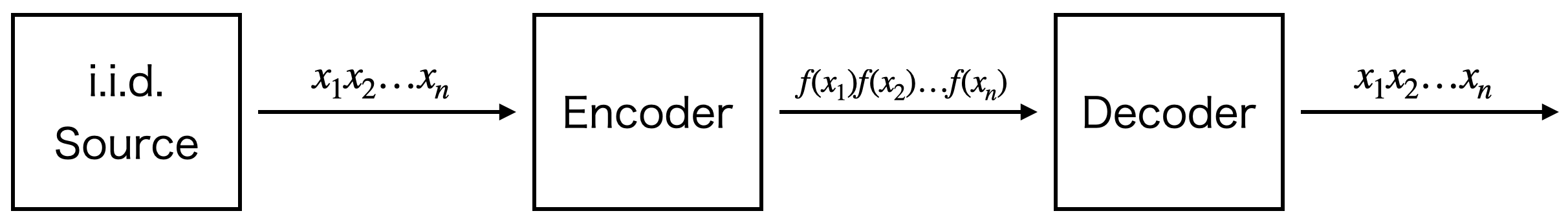
Figure 1: The data compression system in this paper.

For example, consider an i.i.d. source with source alphabet $\mathcal{S}=\{\mathrm{a},\mathrm{b},\mathrm{c},\mathrm{d}\}$, a probability distribution $(\mu(\mathrm{a}),\mu(\mathrm{b}),\mu(\mathrm{c}),\mu(\mathrm{d}))=(0.1,0.2,0.3,0.4)$ and the code table $f^{(\mathrm{I})}$ in Table 1. The average codeword length (per symbol) $L(f^{(\mathrm{I})})$ of the code table $f^{(\mathrm{I})}$ is calculated as

$$L(f^{(\mathrm{I})}) = \mu(\mathrm{a})|f^{(\mathrm{I})}(\mathrm{a})|+\mu(\mathrm{b})|f^{(\mathrm{I})}(\mathrm{b})|+\mu(\mathrm{c})|f^{(\mathrm{I})}(\mathrm{c})|+\mu(\mathrm{d})|f^{(\mathrm{I})}(\mathrm{d})|=1.9,$$ (1)

where $|\cdot|$ denotes the length of a sequence.

A source sequence $\boldsymbol{x}=x_{1}x_{2}x_{3}x_{4}x_{5}=\mathrm{adbac}$ is encoded to $f^{(\mathrm{I})}(\boldsymbol{x})=f^{(\mathrm{I})}(\mathrm{a})f^{(\mathrm{I})}(\mathrm{d})f^{(\mathrm{I})}(\mathrm{b})f^{(\mathrm{I})}(\mathrm{a})\allowbreak f^{(\mathrm{I})}(\mathrm{c})=000100100001$. The code table $f^{(\mathrm{I})}$ is prefix-free; that is, for any two distinct symbols $s$ and $s^{\prime}$, $f(s)$ is not a prefix of $f(s^{\prime})$. Therefore, in the decoding process, the decoder can uniquely determine $x_{1}=\mathrm{a}$ immediately after reading the prefix $f^{(\mathrm{I})}(\mathrm{a})=000$ of $f^{(\mathrm{I})}(\boldsymbol{x})$. Also, the decoder can uniquely determine $x_{1}x_{2}=\mathrm{a}\mathrm{d}$ immediately after reading the prefix $f^{(\mathrm{I})}(\mathrm{a})f^{(\mathrm{I})}(\mathrm{d})=0001$ of $f^{(\mathrm{I})}(\boldsymbol{x})$. In general, a code table $f$ is called an instantaneous code if for any source sequence $\boldsymbol{x}=x_{1}x_{2}\ldots x_{n}$ and its any prefix $x_{1}x_{2}\ldots x_{l}$, the decoder can uniquely recover $x_{1}x_{2}\ldots x_{l}$ immediately after reading the prefix $f(x_{1})f(x_{2})\ldots f(x_{l})$. In fact, the code table $f^{(\mathrm{I})}$ is an instantaneous code.

Table 1: An example of a code table.

$s\in\mathcal{S}$	$f^{(\mathrm{I})}(s)$
a	000
b	001
c	01
d	1

Huffman proposed an algorithm to construct an instantaneous code that achieved the optimal (minimum) average codeword length for a given probability distribution $(\mu(s_{1}),\mu(s_{2}),\ldots,\allowbreak\mu(s_{\sigma}))$ [1]. A code table constructed by Huffman’s algorithm is called a Huffman code. Namely, a Huffman code achieves the optimal average codeword length in the class of instantaneous codes. McMillan’s theorem[2] implies that Huffman code is optimal also in the class of uniquely decodable codes (with a single code table). The code table $f^{(\mathrm{I})}$ in Table 1 is a Huffman code for the probability distribution $(\mu(\mathrm{a}),\mu(\mathrm{b}),\mu(\mathrm{c}),\mu(\mathrm{d}))=(0.1,0.2,0.3,0.4)$.

In 2015, Yamamoto, Tsuchihashi, and Honda[3] proposed binary AIFV code that can achieve a shorter average codeword length than the Huffman code. An AIFV code uses a time-variant encoder consisting of two code tables $f_{0},f_{1}$ and allows at most $2$-bit delay for decoding. We omit details of the definition of AIFV code here and show an example of an AIFV code $F^{(\mathrm{II})}$ in Table 2. In the encoding process of $\boldsymbol{x}=x_{1}x_{2}\ldots x_{n}$ with the AIFV code $F^{(\mathrm{II})}$, the first symbol $x_{1}$ is encoded with the code table $f_{0}$. For $i=2,3,\ldots,n$, if $x_{i-1}$ is encoded with the code table $f_{j}$, then $x_{i}$ is encoded with the code table $f_{\mathrm{\tau}_{j}(x_{i-1})}$. For example, a source sequence $\boldsymbol{x}=x_{1}x_{2}x_{3}x_{4}x_{5}=\mathrm{adbac}$ is encoded to $f_{0}(\mathrm{a})f_{0}(\mathrm{d})f_{1}(\mathrm{b})f_{1}(\mathrm{a})f_{0}(\mathrm{c})=100111110001$.

AIFV code $F^{(\mathrm{II})}$ is not an instantaneous code because the decoder cannot uniquely determine whether $x_{1}x_{2}=\mathrm{a}\mathrm{d}$ or not at the time of reading $f_{0}(\mathrm{a})f_{0}(\mathrm{d})=1001$ (there are still two possibilities, $\boldsymbol{x}=\mathrm{aa}\ldots$ and $\boldsymbol{x}=\mathrm{ad}\ldots$). However, the decoder can distinguish them by reading the following two bits; that is, the decoder can uniquely determine $x_{1}x_{2}=\mathrm{a}\mathrm{d}$ immediately after reading $f_{0}(\mathrm{a})f_{0}(\mathrm{d})11=100111$. Similarly, when the decoder reads the prefix $f_{0}(\mathrm{a})f_{0}(\mathrm{d})f_{1}(\mathrm{b})f_{1}(\mathrm{b})=10011111$, the decoder cannot uniquely determine whether $x_{1}x_{2}x_{3}x_{4}=\mathrm{a}\mathrm{d}\mathrm{b}\mathrm{b}$ or not because there are still two possibilities, $\boldsymbol{x}=\mathrm{adbb}\ldots$ and $\boldsymbol{x}=\mathrm{adba}\ldots$. Also, in this case, the decoder can distinguish them by reading the following two bits, that is, the decoder can uniquely determine $x_{1}x_{2}x_{3}x_{4}\neq\mathrm{a}\mathrm{d}\mathrm{b}\mathrm{b}$ immediately after reading $f_{0}(\mathrm{a})f_{0}(\mathrm{d})f_{1}(\mathrm{b})f_{1}(\mathrm{b})00=1001111100$ since a $00$ cannot follow after encoding $\mathrm{b}$ with $f_{1}$ in the AIFV code $F^{(\mathrm{II})}$. In general, for the AIFV code $F^{(\mathrm{II})}$, the following condition holds for any source sequence $\boldsymbol{x}=x_{1}x_{2}\ldots x_{n}$: at the time immediately after the decoder reads the prefix $b_{1}b_{2}\ldots b_{k}$ of the codeword sequence $f(\boldsymbol{x})$, if $b_{1}b_{2}\ldots b_{k}=f(x^{\prime}_{1})f(x^{\prime}_{2})\ldots f(x^{\prime}_{l})$, then the decoder can uniquely determine whether $x^{\prime}_{1}x^{\prime}_{2}\ldots x^{\prime}_{l}$ is a prefix of the original source sequence $\boldsymbol{x}$ or not by reading the following $2$ bits. Namely, $F^{(\mathrm{II})}$ is a $2$-bit delay decodable code (defined formally in Subsection 2.2).

The average codeword length of an AIFV code $F(f_{0},f_{1},\mathrm{\tau}_{0},\mathrm{\tau}_{1})$ is calculated as follows. Let $I_{i}\in\{0,1\}$ be the index of the code table used to encode the $i$-th symbol of the source sequence, for $i=1,2,3,\ldots$. Then $I_{i},i=1,2,3,\ldots$ is a Markov process. Let $(\pi_{0},\pi_{1})$ be the stationary probability of the Markov process, that is,

$$\pi_{0}=\frac{Q_{1,0}}{Q_{0,1}+Q_{1,0}},\quad\pi_{1}=\frac{Q_{0,1}}{Q_{0,1}+Q_{1,0}},$$ (2)

where $Q_{i,j}$ is the probability of using $f_{j}$ immediately after using $f_{i}$, for $i,j\in\{0,1\}$. Then the average codeword length $L(F)$ of an AIFV code $F$ is $L(F)=\pi_{0}L_{0}(F)+\pi_{1}L_{1}(F)$, where $L_{0}(F)$ (resp. $L_{1}(F)$) is the average codeword length of the single code table $f_{0}$ (resp. $f_{1}$). Thus, the average codeword length of the AIFV code $F^{(\mathrm{II})}$ in Table 2 is

$$L(F^{(\mathrm{II})})=\frac{Q_{1,0}}{Q_{0,1}+Q_{1,0}}L_{0}(F)+\frac{Q_{0,1}}{Q_{0,1}+Q_{1,0}}L_{1}(F)=1.86666\ldots,$$ (3)

which is shorter than $L(f^{(I)})$ of the Huffman code $f^{(\mathrm{I})}$ in Table 2 (cf. (1)). We [4] indicate that binary AIFV code achieves the optimal average codeword length in the class of $2$-bit delay decodable code with two code tables.

Table 2: An example of an AIFV code $F^{(\mathrm{II})}(f_{0},f_{1},\mathrm{\tau}_{0},\mathrm{\tau}_{1})$.

$s\in\mathcal{S}$	$f_{0}(s)$	$\mathrm{\tau}_{0}(s)$	$f_{1}(s)$	$\mathrm{\tau}_{1}(s)$
a	100	0	1100	0
b	00	0	11	1
c	01	0	01	0
d	1	1	10	0

Binary AIFV code is generalized to binary AIFV-$m$ code, which can achieve a shorter average codeword length than binary AIFV code for $m\geq 3$, allowing $m$ code tables and at most $m$-bit decoding delay [5]. Analyses of the worst-case redundancy of AIFV and AIFV-$m$ codes are studied in the literature[5, 6] for $m=2,3,4,5$. The papers [7, 8, 13, 11, 10, 12, 15, 16, 17, 19, 20, 9, 14, 18] propose the code construction and coding method of AIFV and AIFV-$m$ codes. Extensions of AIFV-$m$ codes are proposed in the papers [21, 22].

As stated above, there exist $m$-bit delay decodable codes with a finite number of code tables better than Huffman code for $m\geq 2$. However, it is not known for the case $m=1$. In this paper, we prove that there are no $1$-bit delay decodable codes with a finite number of code tables, which achieves a shorter average codeword length than the Huffman code. Namely, Huffman code is optimal in the class of $1$-bit delay decodable codes with a finite number of code tables.

2 Preliminaries

First, we define some notations as follows. Let $|\mathcal{A}|$ denote the cardinality of a finite set $\mathcal{A}$. Let $\mathcal{A}\times\mathcal{B}$ denote the set of all ordered pairs $(a,b)$, $a\in\mathcal{A}$ and $b\in\mathcal{B}$, that is, $\mathcal{A}\times\mathcal{B}:=\{(a,b):a\in\mathcal{A},b\in\mathcal{B}\}$. Let $\mathcal{A}^{k}$ denote the set of all sequences of length $k$ over a set $\mathcal{A}$, and let $\mathcal{A}^{\ast}$ denote the set of all sequences of finite length over a set $\mathcal{A}$, that is, $\mathcal{A}^{\ast}:=\mathcal{A}^{0}\cup\mathcal{A}^{1}\cup\mathcal{A}^{2}\cup\cdots$. The empty sequence is denoted by $\lambda$. The length of a sequence $\boldsymbol{x}$ is denoted by $|\boldsymbol{x}|$. In particular, $|\lambda|=0$. We say $\boldsymbol{x}\preceq\boldsymbol{y}$ if $\boldsymbol{x}$ is a prefix of $\boldsymbol{y}$, that is, there exists a sequence $\boldsymbol{z}$, possibly $\boldsymbol{z}=\lambda$, such that $\boldsymbol{y}=\boldsymbol{x}\boldsymbol{z}$. For a non-empty sequence $\boldsymbol{x}=x_{1}x_{2}\ldots x_{n}$, we define $\mathrm{suf}(\boldsymbol{x}):=x_{2}x_{3}\ldots x_{n}$, that is, $\mathrm{suf}(\boldsymbol{x})$ is the sequence obtained by deleting the first letter $x_{1}$ from $\boldsymbol{x}$. Some notations used in this paper are listed in Appendix B.

2.1 Code-Tuple

We formalize a time-variant encoder with a finite number of code tables as a code-tuple. An $m$-code-tuple consists of $m$ code tables $f_{0},f_{1}\ldots,f_{m-1}$ from $\mathcal{S}$ to $\mathcal{C}^{\ast}$ and $m$ mappings $\mathrm{\tau}_{0},\mathrm{\tau}_{1},\ldots,\mathrm{\tau}_{m-1}$ from $\mathcal{S}$ to $[m]:=\{0,1,2,\ldots,m-1\}$. The $m$ mappings $\mathrm{\tau}_{0},\mathrm{\tau}_{1},\ldots,\mathrm{\tau}_{m-1}$ determine which code table to use to encode the $i$-th symbol $x_{i}$ of a source sequence: if the previous symbol $x_{i-1}$ is encoded with $f_{j}$, then the current symbol $x_{i}$ is encoded with $f_{\mathrm{\tau}_{j}(x_{i-1})}$.

Definition 1

Let $m$ be a positive integer. An $m$-code-tuple $F(f_{i},\mathrm{\tau}_{i}:i\in[m])$ is a tuple of $m$ mappings $f_{i}:\mathcal{S}\rightarrow\mathcal{C}^{\ast},i\in[m]$ and $m$ mappings $\mathrm{\tau}_{i}:\mathcal{S}\rightarrow[m],i\in[m]$.

Let $\mathscr{F}^{(m)}$ denote the set of all $m$-code-tuples and define $\mathscr{F}:=\mathscr{F}^{(1)}\cup\mathscr{F}^{(2)}\cup\mathscr{F}^{(3)}\cup\cdots$. An element of $\mathscr{F}$ is called a code-tuple. We sometimes write $F(f_{i},\mathrm{\tau}_{i}:i\in[m])$ as $F(f,\mathrm{\tau})$ or $F$ for simplicity. For $F\in\mathscr{F}^{(m)}$, let $|F|$ denote the number of code tables of $F$, that is, $|F|:=m$. We write $[|F|]$ as $[F]$ for simplicity.

Table 3: Four examples of a code-tuple $F^{(\alpha)}(f^{(\alpha)},\mathrm{\tau}^{(\alpha)}),F^{(\beta)}(f^{(\beta)},\mathrm{\tau}^{(\beta)}),F^{(\gamma)}(f^{(\gamma)},\mathrm{\tau}^{(\gamma)})$, and $F^{(\delta)}(f^{(\delta)},\mathrm{\tau}^{(\delta)})$.

$s\in\mathcal{S}$	$f^{(\alpha)}_{0}(s)$	$\mathrm{\tau}^{(\alpha)}_{0}(s)$	$f^{(\alpha)}_{1}(s)$	$\mathrm{\tau}^{(\alpha)}_{1}(s)$	$f^{(\alpha)}_{2}(s)$	$\mathrm{\tau}^{(\alpha)}_{2}(s)$	$f^{(\alpha)}_{3}(s)$	$\mathrm{\tau}^{(\alpha)}_{3}(s)$
a	$\lambda$	1	110	3	010	0	$\lambda$	3
b	000	1	$\lambda$	2	011	1	$\lambda$	3
c	001	2	110	1	10	2	$\lambda$	3

$s\in\mathcal{S}$	$f^{(\beta)}_{0}(s)$	$\mathrm{\tau}^{(\beta)}_{0}(s)$	$f^{(\beta)}_{1}(s)$	$\mathrm{\tau}^{(\beta)}_{1}(s)$	$f^{(\beta)}_{2}(s)$	$\mathrm{\tau}^{(\beta)}_{2}(s)$
a	11	2	0110	1	10	2
b	$\lambda$	1	0110	2	11	1
c	101	1	01	1	1000	0
d	1011	1	0111	2	1001	1
e	1101	2	01110	2	11100	2

$s\in\mathcal{S}$	$f^{(\gamma)}_{0}(s)$	$\mathrm{\tau}^{(\gamma)}_{0}(s)$	$f^{(\gamma)}_{1}(s)$	$\mathrm{\tau}^{(\gamma)}_{1}(s)$	$f^{(\gamma)}_{2}(s)$	$\mathrm{\tau}^{(\gamma)}_{2}(s)$
a	111	2	1100	1	01	2
b	0	1	1101	2	10	1
c	1010	1	10	1	000	0
d	10110	1	1111	2	0010	1
e	11011	2	11101	2	11001	2

$s\in\mathcal{S}$	$f^{(\delta)}_{0}(s)$	$\mathrm{\tau}^{(\delta)}_{0}(s)$	$f^{(\delta)}_{1}(s)$	$\mathrm{\tau}^{(\delta)}_{1}(s)$	$f^{(\delta)}_{2}(s)$	$\mathrm{\tau}^{(\delta)}_{2}(s)$
a	111	2	1001	1	01	2
b	01	1	101	2	101	1
c	10101	1	01	1	000	0
d	101101	1	111	2	00101	1
e	11011	2	1101	2	11001	2

Example 1

Table 3 shows four examples of a code-tuple $F^{(\alpha)}(f^{(\alpha)},\mathrm{\tau}^{(\alpha)})\in\mathscr{F}^{(4)}$ for $\mathcal{S}=\{\mathrm{a},\mathrm{b},\mathrm{c}\}$, and $F^{(\beta)}(f^{(\beta)},\mathrm{\tau}^{(\beta)}),F^{(\gamma)}(f^{(\gamma)},\mathrm{\tau}^{(\gamma)}),F^{(\delta)}(f^{(\delta)},\mathrm{\tau}^{(\delta)})\in\mathscr{F}^{(3)}$ for $\mathcal{S}=\{\mathrm{a},\mathrm{b},\mathrm{c},\mathrm{d},\mathrm{e}\}$.

In encoding $x_{1}x_{2}\ldots x_{n}\in\mathcal{S}^{\ast}$ with a $F(f,\mathrm{\tau})\in\mathscr{F}$, the mappings $\mathrm{\tau}_{0},\mathrm{\tau}_{1},\ldots,\mathrm{\tau}_{|F|-1}$ determine which code table to use to encode $x_{i}$ for $i=2,3,\ldots,n$. However, there are choices of which code table to use for the first symbol $x_{1}$. For $i\in[F]$ and $\boldsymbol{x}\in\mathcal{S}^{\ast}$, we define $f^{\ast}_{i}(\boldsymbol{x})\in\mathcal{C}^{\ast}$ as the codeword sequence in the case where $x_{1}$ is encoded with $f_{i}$. Namely, $f^{\ast}_{i}(x_{1}x_{2}x_{3}\ldots)=f_{i}(x_{1})f_{\mathrm{\tau}_{i}(x_{1})}(x_{2})f_{\mathrm{\tau}_{\mathrm{\tau}_{i}(x_{1})}(x_{2})}(x_{3})\ldots$. Also, we define $\mathrm{\tau}^{\ast}_{i}(\boldsymbol{x})\in[F]$ as the index of the code table to be used next after encoding $\boldsymbol{x}$ in the case where $x_{1}$ is encoded with $f_{i}$. We give formal definitions of $f^{\ast}_{i}$ and $\mathrm{\tau}^{\ast}_{i}$ in the following Definition 2 as recursive formulas.

Definition 2

For $F(f,\mathrm{\tau})\in\mathscr{F}$ and $i\in[F]$, we define a mapping $f_{i}^{\ast}:\mathcal{S}^{\ast}\rightarrow\mathcal{C}^{\ast}$ and a mapping $\mathrm{\tau}_{i}^{\ast}:\mathcal{S}^{\ast}\rightarrow[F]$ as follows.

$$f_{i}^{\ast}(\boldsymbol{x})=\begin{cases}\lambda&\,\,\text{if}\,\,\boldsymbol{x}=\lambda,\\ f_{i}(x_{1})f_{\mathrm{\tau}_{i}(x_{1})}^{\ast}(\mathrm{suf}(\boldsymbol{x}))&\,\,\text{if}\,\,\boldsymbol{x}\neq\lambda,\\ \end{cases}$$ (4)

$$\mathrm{\tau}_{i}^{\ast}(\boldsymbol{x})=\begin{cases}i&\,\,\text{if}\,\,\boldsymbol{x}=\lambda,\\ \mathrm{\tau}^{\ast}_{\mathrm{\tau}_{i}(x_{1})}(\mathrm{suf}(\boldsymbol{x}))&\,\,\text{if}\,\,\boldsymbol{x}\neq\lambda,\\ \end{cases}$$ (5)

for $\boldsymbol{x}=x_{1}x_{2}\ldots x_{n}\in\mathcal{S}^{\ast}$.

Example 2

Let $F(f,\mathrm{\tau})$ be $F^{(\beta)}(f^{(\beta)},\mathrm{\tau}^{(\beta)})$ of Table 3. We have

$$f_{2}^{\ast}(\mathrm{baed}) = f_{2}(\mathrm{b})f_{1}^{\ast}(\mathrm{aed})$$ (6)

$$= f_{2}(\mathrm{b})f_{1}(\mathrm{a})f_{1}^{\ast}(\mathrm{ed})$$ (7)

$$= f_{2}(\mathrm{b})f_{1}(\mathrm{a})f_{1}(\mathrm{e})f_{2}^{\ast}(\mathrm{d})$$ (8)

$$= f_{2}(\mathrm{b})f_{1}(\mathrm{a})f_{1}(\mathrm{e})f_{2}(\mathrm{d})f_{1}^{\ast}(\lambda)$$ (9)

$$= f_{2}(\mathrm{b})f_{1}(\mathrm{a})f_{1}(\mathrm{e})f_{2}(\mathrm{d})$$ (10)

$$= 110110011101001.$$ (11)

$$\mathrm{\tau}_{2}^{\ast}(\mathrm{baed})=\mathrm{\tau}^{\ast}_{1}(\mathrm{aed})=\mathrm{\tau}^{\ast}_{1}(\mathrm{ed})=\mathrm{\tau}^{\ast}_{2}(\mathrm{d})=\mathrm{\tau}^{\ast}_{1}(\mathrm{\lambda})=1.$$ (12)

Directly from Definition 2, we obtain the following lemma.

Lemma 1

For any $F(f,\mathrm{\tau})\in\mathscr{F}$ and $i\in[F]$, the following conditions (i)–(iii) hold.

1. For any $\boldsymbol{x},\boldsymbol{y}\in\mathcal{S}^{\ast}$, $f_{i}^{\ast}(\boldsymbol{x}\boldsymbol{y})=f_{i}^{\ast}(\boldsymbol{x})f^{\ast}_{\mathrm{\tau}_{i}^{\ast}(\boldsymbol{x})}(\boldsymbol{y})$.

2. For any $\boldsymbol{x},\boldsymbol{y}\in\mathcal{S}^{\ast}$, $\mathrm{\tau}_{i}^{\ast}(\boldsymbol{x}\boldsymbol{y})=\mathrm{\tau}^{\ast}_{\mathrm{\tau}^{\ast}_{i}(\boldsymbol{x})}(\boldsymbol{y})$.

3. For any $\boldsymbol{x},\boldsymbol{y}\in\mathcal{S}^{\ast}$, if $\boldsymbol{x}\preceq\boldsymbol{y}$, then $f^{\ast}_{i}(\boldsymbol{x})\preceq f^{\ast}_{i}(\boldsymbol{y})$.

For the code-tuple $F^{(\alpha)}$ in Table 3, we can see that ${{f^{(\alpha)}_{3}}^{\ast}}(\boldsymbol{x})=\lambda$ for any $\boldsymbol{x}\in\mathcal{S}^{\ast}$. To distinguish such abnormal and useless code-tuples from the others, we introduce a class $\mathscr{F}_{\mathrm{ext}}$ in the following Definition 3.

Definition 3

We define $\mathscr{F}_{\mathrm{ext}}$ as the set of all $F(f,\mathrm{\tau})\in\mathscr{F}$ such that for any $i\in[F]$, there exists $\boldsymbol{x}\in\mathcal{S}^{\ast}$ such that $|f^{\ast}_{i}(\boldsymbol{x})|>0$.

Directly from Definition 3, for any $F(f,\mathrm{\tau})\in\mathscr{F}_{\mathrm{ext}},i\in[F]$ and an integer $k\geq 0$, there exists $\boldsymbol{x}\in\mathcal{S}^{\ast}$ such that $|f^{\ast}_{i}(\boldsymbol{x})|\geq k$. Namely, we can extend $f^{\ast}_{i}(\boldsymbol{x})$ as long as we want by appending symbols to $\boldsymbol{x}$ appropriately. The subscription "$\mathrm{ext}$" of $\mathscr{T}_{\mathrm{ext}}$ is an abbreviation of “extendable.”

Example 3

Consider $F^{(\alpha)},F^{(\beta)},F^{(\gamma)}$, and $F^{(\delta)}$ of Table 3. We have $F^{(\alpha)}\not\in\mathscr{F}_{\mathrm{ext}}$ because $|{{f^{(\alpha)}_{3}}^{\ast}}(\boldsymbol{x})|=0$ for any $\boldsymbol{x}\in\mathcal{S}^{\ast}$. On the other hand, $F^{(\beta)},F^{(\gamma)},F^{(\delta)}\in\mathscr{F}_{\mathrm{ext}}$.

2.2 $k$-bit Delay Decodable Code-Tuple

Let $F(f,\mathrm{\tau})\in\mathscr{F}$ and $i\in[F]$. Consider a situation that a source sequence $\boldsymbol{x^{\prime}}\in\mathcal{S}^{\ast}$ is encoded with $F$ starting from the code table $f_{i}$. Then the source sequence $\boldsymbol{x^{\prime}}$ is encoded to the codeword sequence $f^{\ast}_{i}(\boldsymbol{x^{\prime}})$, and the decoder reads it bit by bit from the beginning. Let $\boldsymbol{b}\preceq f(\boldsymbol{x^{\prime}})$ be the sequence the decoder has read by a certain moment of the decoding process. If $\boldsymbol{b}=f(\boldsymbol{x})$ for some $\boldsymbol{x}\in\mathcal{S}^{\ast}$, then there are two possible cases, $\boldsymbol{x}\preceq\boldsymbol{x^{\prime}}$ and $\boldsymbol{x}\not\preceq\boldsymbol{x^{\prime}}$. We say that $F$ is $k$-bit delay decodable if it is always possible for the decoder to distinguish the two cases, $\boldsymbol{x}\preceq\boldsymbol{x^{\prime}}$ and $\boldsymbol{x}\not\preceq\boldsymbol{x^{\prime}}$, by reading the following $k$ bits $\boldsymbol{c}\in\mathcal{C}^{k}$ of the codeword sequence $f(\boldsymbol{x})$, that is, for any pair $(\boldsymbol{x},\boldsymbol{c})\in\mathcal{S}^{\ast}\times\mathcal{C}^{k}$, the decoder can distinguish the two cases, $\boldsymbol{x}\preceq\boldsymbol{x^{\prime}}$ and $\boldsymbol{x}\not\preceq\boldsymbol{x^{\prime}}$ according to the pair $(\boldsymbol{x},\boldsymbol{c})$. Thus, $F$ is $k$-bit delay decodable if and only if for any pair $(\boldsymbol{x},\boldsymbol{c})\in\mathcal{S}^{\ast}\times\mathcal{C}^{k}$, it holds that $(\boldsymbol{x},\boldsymbol{c})$ is $f^{\ast}_{i}$-positive or $f^{\ast}_{i}$-negative defined as follows.

Definition 4

Let $F(f,\mathrm{\tau})\in\mathscr{F}$ and $i\in[F]$.

1. A pair $(\boldsymbol{x},\boldsymbol{c})\in\mathcal{S}^{\ast}\times\mathcal{C}^{\ast}$ is said to be $f^{\ast}_{i}$-positive if for any $\boldsymbol{x^{\prime}}\in\mathcal{S}^{\ast}$, if $f^{\ast}_{i}(\boldsymbol{x})\boldsymbol{c}\preceq f^{\ast}_{i}(\boldsymbol{x^{\prime}})$, then $\boldsymbol{x}\preceq\boldsymbol{x^{\prime}}$.

2. A pair $(\boldsymbol{x},\boldsymbol{c})\in\mathcal{S}^{\ast}\times\mathcal{C}^{\ast}$ is said to be $f^{\ast}_{i}$-negative if for any $\boldsymbol{x^{\prime}}\in\mathcal{S}^{\ast}$, if $f^{\ast}_{i}(\boldsymbol{x})\boldsymbol{c}\preceq f^{\ast}_{i}(\boldsymbol{x^{\prime}})$, then $\boldsymbol{x}\not\preceq\boldsymbol{x^{\prime}}$.

Definition 5

Let $F(f,\mathrm{\tau})\in\mathscr{F}$ and let $k\geq 0$ be an integer. The code-tuple $F$ is said to be $k$-bit delay decodable if for any $i\in[F]$ and $(\boldsymbol{x},\boldsymbol{c})\in\mathcal{S}^{\ast}\times\mathcal{C}^{k}$, the pair $(\boldsymbol{x},\boldsymbol{c})$ is $f^{\ast}_{i}$-positive or $f^{\ast}_{i}$-negative. For an integer $k\geq 0$, we define $\mathscr{F}_{k\text{-}\mathrm{dec}}$ as the set of all $k$-bit delay decodable code-tuples.

Note that it is possible that a $(\boldsymbol{x},\boldsymbol{c})\in\mathcal{S}^{\ast}\times\mathcal{C}^{\ast}$ is $f^{\ast}_{i}$-positive and $f^{\ast}_{i}$-negative simultaneously. A $(\boldsymbol{x},\boldsymbol{c})\in\mathcal{S}^{\ast}\times\mathcal{C}^{\ast}$ is $f^{\ast}_{i}$-positive and $f^{\ast}_{i}$-negative simultaneously if and only if there is no sequence $\boldsymbol{x^{\prime}}$ satisfying $f^{\ast}_{i}(\boldsymbol{x})\boldsymbol{c}\preceq f^{\ast}_{i}(\boldsymbol{x^{\prime}})$.

In fact, the classes $\mathscr{F}_{k\text{-}\mathrm{dec}},k=0,1,2,\ldots$ form a hierarchical structure $\mathscr{F}_{0\text{-}\mathrm{dec}}\subseteq\mathscr{F}_{1\text{-}\mathrm{dec}}\subseteq\mathscr{F}_{2\text{-}\mathrm{dec}}\subseteq\cdots.$ Namely, the following Lemma 2 holds.

Lemma 2

For any two non-negative integers $k,k^{\prime}$ such that $k\leq k^{\prime}$, we have $\mathscr{F}_{k\text{-}\mathrm{dec}}\subseteq\mathscr{F}_{k^{\prime}\text{-}\mathrm{dec}}$.

Proof of Lemma 2: Let $F(f,\mathrm{\tau})\in\mathscr{F}_{k\text{-}\mathrm{dec}}$. Fix $i\in[F]$ and $(\boldsymbol{x},\boldsymbol{c^{\prime}})\in\mathcal{S}^{\ast}\times\mathcal{C}^{k^{\prime}}$ arbitrarily. It suffices to prove that $(\boldsymbol{x},\boldsymbol{c^{\prime}})$ is $f^{\ast}_{i}$-positive or $f^{\ast}_{i}$-negative.

Let $\boldsymbol{c}$ be the prefix of $\boldsymbol{c^{\prime}}$ of length $k$. Then for any $\boldsymbol{x^{\prime}}\in\mathcal{S}^{\ast}$ such that $f^{\ast}_{i}(\boldsymbol{x})\boldsymbol{c^{\prime}}\preceq f^{\ast}_{i}(\boldsymbol{x^{\prime}})$, we have $f^{\ast}_{i}(\boldsymbol{x})\boldsymbol{c}\preceq f^{\ast}_{i}(\boldsymbol{x})\boldsymbol{c^{\prime}}\preceq f^{\ast}_{i}(\boldsymbol{x^{\prime}}$). Namely, $f^{\ast}_{i}(\boldsymbol{x})\boldsymbol{c^{\prime}}\preceq f^{\ast}_{i}(\boldsymbol{x^{\prime}})$ implies $f^{\ast}_{i}(\boldsymbol{x})\boldsymbol{c}\preceq f^{\ast}_{i}(\boldsymbol{x^{\prime}})$. Hence, from Definition 4, if $(\boldsymbol{x},\boldsymbol{c^{\prime}})$ is $f^{\ast}_{i}$-positive (resp. $f^{\ast}_{i}$-negative), then also $(\boldsymbol{x},\boldsymbol{c})$ is $f^{\ast}_{i}$-positive (resp. $f^{\ast}_{i}$-negative), respectively. Therefore, it follows that $F(f,\mathrm{\tau})\in\mathscr{F}_{k^{\prime}\text{-}\mathrm{dec}}$ from $F(f,\mathrm{\tau})\in\mathscr{F}_{k\text{-}\mathrm{dec}}$. $\Box$

Example 4

Consider $F^{(\alpha)},F^{(\beta)},F^{(\gamma)}$, and $F^{(\delta)}$ of Table 3. We have $F^{(\alpha)}\in\mathscr{F}_{2\text{-}\mathrm{dec}}\setminus\mathscr{F}_{1\text{-}\mathrm{dec}}$, $F^{(\beta)}\in\mathscr{F}_{1\text{-}\mathrm{dec}}\setminus\mathscr{F}_{0\text{-}\mathrm{dec}}$, and $F^{(\gamma)},F^{(\delta)}\in\mathscr{F}_{0\text{-}\mathrm{dec}}$.

We remark that a $k$-bit delay decodable code-tuple is not necessarily uniquely decodable. For example, for the code-tuple $F^{(\beta)}\in\mathscr{F}_{1\text{-}\mathrm{dec}}$, we have $f^{\ast}_{0}(\mathrm{ac})=111000=f^{\ast}_{0}(\mathrm{acb})$. In general, it is possible that the decoder cannot uniquely recover the last few symbols of the original source sequence because the length of the rest of the codeword sequence is less than $k$ bits. In such a case, we should append additional information to uniquely decode the suffix in practical use.

However, as we show in the following Lemma 3, a $0$-bit delay decodable code-tuple (i.e., an instantaneous code) is always uniquely decodable.

Lemma 3

For any $F(f,\mathrm{\tau})\in\mathscr{F}_{0\text{-}\mathrm{dec}}$ and $i\in[F]$, the following conditions (i) and (ii) hold.

1. For any $\boldsymbol{x}\in\mathcal{S}^{\ast}$, the pair $(\boldsymbol{x},\lambda)$ is $f^{\ast}_{i}$-positive.

2. $f^{\ast}_{i}$ is injective.

Proof of Lemma 3: (Proof of (i)) From $F\in\mathscr{F}_{0\text{-}\mathrm{dec}}$, the pair $(\boldsymbol{x},\lambda)$ is $f^{\ast}_{i}$-positive or $f^{\ast}_{i}$-negative. However, since $f^{\ast}_{i}(\boldsymbol{x})\preceq f^{\ast}_{i}(\boldsymbol{x})$ and $\boldsymbol{x}\preceq\boldsymbol{x}$, the pair $(\boldsymbol{x},\lambda)$ must be $f^{\ast}_{i}$-positive.

(Proof of (ii)) From (i), we have

$${}^{\forall}\boldsymbol{x},\boldsymbol{x^{\prime}}\in\mathcal{S}^{\ast},\big{(}f^{\ast}_{i}(\boldsymbol{x})\preceq f^{\ast}_{i}(\boldsymbol{x^{\prime}})\Rightarrow\boldsymbol{x}\preceq\boldsymbol{x^{\prime}}\big{)}.$$ (13)

Choose $\boldsymbol{y},\boldsymbol{y^{\prime}}\in\mathcal{S}^{\ast}$ such $f^{\ast}_{i}(\boldsymbol{y})=f^{\ast}_{i}(\boldsymbol{y^{\prime}})$ arbitrarily. Then we have $f^{\ast}_{i}(\boldsymbol{y})\preceq f^{\ast}_{i}(\boldsymbol{y^{\prime}})$ and $f^{\ast}_{i}(\boldsymbol{y^{\prime}})\preceq f^{\ast}_{i}(\boldsymbol{y})$. From (13), we obtain $\boldsymbol{y}\preceq\boldsymbol{y^{\prime}}$ and $\boldsymbol{y^{\prime}}\preceq\boldsymbol{y}$, that is, $\boldsymbol{y}=\boldsymbol{y^{\prime}}$. Consequently, $f^{\ast}_{i}$ is injective. $\Box$.

For $F(f,\mathrm{\tau})\in\mathscr{F}$ and $i\in[F]$, $f_{i}$ is said to be prefix-free if for any $s,s^{\prime}\in\mathcal{S}$, if $f_{i}(s)\preceq f_{i}(s^{\prime})$, then $s=s^{\prime}$. A $0$-bit delay decodable code-tuple is characterized as a code-tuple all of which code tables are prefix-free.

Lemma 4

A $F(f,\mathrm{\tau})\in\mathscr{F}$ satisfies $F\in\mathscr{F}_{0\text{-}\mathrm{dec}}$ if and only if for any $i\in[F]$, $f_{i}$ is prefix-free.

Proof of Lemma 4: (Proof of “only if”) Assume $F\in\mathscr{F}_{0\text{-}\mathrm{dec}}$ and choose $i\in[F]$ arbitrarily. From Lemma 3 (i), the pair $(\boldsymbol{x},\lambda)$ is $f^{\ast}_{i}$-positive. Thus, (13) holds. In particular, we have

$${}^{\forall}s,s^{\prime}\in\mathcal{S},\big{(}f^{\ast}_{i}(s)\preceq f^{\ast}_{i}(s^{\prime})\Rightarrow s\preceq s^{\prime}\big{)}.$$ (14)

Since $s\preceq s^{\prime}$ implies $s=s^{\prime}$, $f_{i}$ is prefix-free.

(Proof of “if”) Assume that for any $i\in[F]$, $f_{i}$ is prefix-free. Fix $i\in[F]$ arbitrarily. To prove $F\in\mathscr{F}_{0\text{-}\mathrm{dec}}$, it suffices to prove (13). We prove it by induction for $|\boldsymbol{x}|$.

For the case $|\boldsymbol{x}|=0$, clearly we have $\boldsymbol{x}\preceq\boldsymbol{x^{\prime}}$ for any $\boldsymbol{x^{\prime}}\in\mathcal{S}^{\ast}$.

Let $l\geq 1$ and assume that (13) is true for the case $|\boldsymbol{x}|<l$ as the induction hypothesis. We prove (13) for the case $|\boldsymbol{x}|=l$. Choose $\boldsymbol{x^{\prime}}\in\mathcal{S}^{\ast}$ such that $f^{\ast}_{i}(\boldsymbol{x})\preceq f^{\ast}_{i}(\boldsymbol{x^{\prime}})$ arbitrarily. Then by (4), we have

$$f_{i}(x_{1})f^{\ast}_{\mathrm{\tau}^{\ast}_{i}(x_{1})}(\mathrm{suf}(\boldsymbol{x}))\preceq f_{i}(x^{\prime}_{1})f^{\ast}_{\mathrm{\tau}^{\ast}_{i}(x^{\prime}_{1})}(\mathrm{suf}(\boldsymbol{x^{\prime}})),$$ (15)

where $\boldsymbol{x}=x_{1}x_{2}\ldots x_{n}$, $\boldsymbol{x^{\prime}}=x^{\prime}_{1}x^{\prime}_{2}\ldots x^{\prime}_{n^{\prime}}$. Thus, $f_{i}(x_{1})\preceq f_{i}(x^{\prime}_{1})$ or $f_{i}(x_{1})\succeq f_{i}(x^{\prime}_{1})$ holds. Hence, since $f_{i}$ is prefix-free, we obtain

$$x_{1}=x^{\prime}_{1}.$$ (16)

From (15) and (16), we have $f_{i}(x_{1})f^{\ast}_{\mathrm{\tau}^{\ast}_{i}(x_{1})}(\mathrm{suf}(\boldsymbol{x}))\preceq f_{i}(x_{1})f^{\ast}_{\mathrm{\tau}^{\ast}_{i}(x^{\prime}_{1})}(\mathrm{suf}(\boldsymbol{x^{\prime}})).$ Thus, we have $f^{\ast}_{\mathrm{\tau}^{\ast}_{i}(x_{1})}(\mathrm{suf}(\boldsymbol{x}))\preceq f^{\ast}_{\mathrm{\tau}^{\ast}_{i}(x^{\prime}_{1})}(\mathrm{suf}(\boldsymbol{x^{\prime}})).$ From the induction hypothesis,

$$\mathrm{suf}(\boldsymbol{x})\preceq\mathrm{suf}(\boldsymbol{x^{\prime}}).$$ (17)

By (16) and (17), we obtain $\boldsymbol{x}\preceq\boldsymbol{x^{\prime}}$. $\Box$

2.3 Average Codeword Length of Code-Tuple

We introduce the average codeword length $L(F)$ of code-tuple $F$. Hereinafter, we fix a probability distribution $\mu$ of source symbols, that is, a real-valued function $\mu:\mathcal{S}\rightarrow\mathbb{R}$ satisfying $\sum_{s\in\mathcal{S}}\mu(s)=1$ and $0<\mu(s)\leq 1$ for any $s\in\mathcal{S}$. Note that we exclude the case where $\mu(s)=0$ for some $s\in\mathcal{S}$ from our consideration without loss of generality.

First, we define the transition probability $Q_{i,j}(F)$ for $F(f,\mathrm{\tau})\in\mathscr{F}$ and $i,j\in[F]$ as the probability of using $f_{j}$ immediately after using $f_{i}$.

Definition 6

For $F(f,\mathrm{\tau})\in\mathscr{F}$ and $i,j\in[F]$, we define the transition probability $Q_{i,j}(F)$ as $Q_{i,j}(F):=\sum_{s\in\mathcal{S},\mathrm{\tau}_{i}(s)=j}\mu(s)$. We also define the transition probability matrix $Q(F)$ as the following $|F|\times|F|$ matrix.

$$Q(F):=\left[\begin{array}[]{cccc}Q_{0,0}(F)&Q_{0,1}(F)&\cdots&Q_{0,|F|-1}(F)\\ Q_{1,0}(F)&Q_{1,1}(F)&\cdots&Q_{1,|F|-1}(F)\\ \vdots&\vdots&\ddots&\vdots\\ Q_{|F|-1,0}(F)&Q_{|F|-1,1}(F)&\cdots&Q_{|F|-1,|F|-1}(F)\end{array}\right].$$ (18)

Fix a $F\in\mathscr{F}$ and Let $I_{i}\in\{0,1\}$ be the index of the code table used to encode the $i$-th symbol of the source sequence in encoding with $F$ for $i=1,2,3,\ldots$. Then $I_{i}\in\{0,1\},i=1,2,3,\ldots$ is a Markov process with the transition probability matrix $Q(F)$. We consider a stationary distribution of the Markov process (i.e., the solution of the simultaneous equations (19) and (20)). The average codeword length $L(F)$ of a code-tuple $F$ depends on a stationary distribution of the Markov process with $Q(F)$. Hence, to define $L(F)$ uniquely, a stationary distribution of the Markov process with $Q(F)$ must be unique. Thus, we define the class $\mathscr{F}_{\mathrm{reg}}$ of all code-tuples such that the Markov process has a unique stationary distribution.

Definition 7

A $F\in\mathscr{F}$ is said to be regular if the following simultaneous equations (19) and (20) have a unique solution $\boldsymbol{\pi}=(\pi_{0},\pi_{1},\ldots,\pi_{|F|-1})$.

$$\boldsymbol{\pi}Q(F)=\boldsymbol{\pi},$$ (19)

$$\sum_{i\in[F]}\pi_{i}=1.$$ (20)

We define $\mathscr{F}_{\mathrm{reg}}$ as the set of all regular code-tuples. For $F\in\mathscr{F}_{\mathrm{reg}}$, we define $\boldsymbol{\pi}(F)=(\pi_{0}(F),\pi_{1}(F),\ldots,\pi_{|F|-1}(F))$ as the unique solution of the simultaneous equations (19) and (20).

For any $F\in\mathscr{F}_{\mathrm{reg}}$, the asymptotical performance (average codeword length per symbol) does not depend on which code table we start encoding: the average codeword length $L(F)$ of a regular code tuple $F\in\mathscr{F}_{\mathrm{reg}}$ is the weighted sum of average codeword lengths of a single code table $f_{0},f_{1},\ldots,f_{|F|-1}$ weighted by the stationary distribution $\boldsymbol{\pi}(F)$.

Definition 8

For $F(f,\mathrm{\tau})\in\mathscr{F}$ and $i\in[F]$, we define the average codeword length $L_{i}(F)$ of a single code table $f_{i}:\mathcal{S}\rightarrow\mathcal{C}^{\ast}$ as $L_{i}(F):=\sum_{s\in\mathcal{S}}|f_{i}(s)|\cdot\mu(s)$. For $F\in\mathscr{F}_{\mathrm{reg}}$, we define the average codeword length $L(F)$ of code-tuple $F$ as $L(F):=\sum_{i\in[F]}\pi_{i}(F)L_{i}(F)$.

Example 5

Let $F(f,\mathrm{\tau})$ be $F^{(\beta)}(f^{(\beta)},\mathrm{\tau}^{(\beta)})$ of Table 3 and let $(\mu(\mathrm{a}),\mu(\mathrm{b}),\mu(\mathrm{c}),\mu(\mathrm{d}),\mu(\mathrm{e}))=(0.1,0.2,0.2,0.2,0.3)$.

We have

$$Q(F)=\left[\begin{array}[]{cccc}0&0.6&0.4\\ 0&0.3&0.7\\ 0.2&0.4&0.4\end{array}\right],$$ (21)

$$L_{0}(F)=2.8,\quad L_{1}(F)=3.9,\quad L_{2}(F)=3.7.$$ (22)

Also, we obtain $\boldsymbol{\pi}(F)=(7/68,26/68,35/68)$ by solving the simultaneous equations (19) and (20). Therefore, the average codeword length $L(F)$ of the code-tuple $F$ is given as

$$L(F) = \pi_{0}(F)L_{0}(F)+\pi_{1}(F)L_{1}(F)+\pi_{2}(F)L_{2}(F)$$ (23)

$$= \frac{7\cdot 2.8+26\cdot 3.9+35\cdot 3.7}{68}$$ (24)

$$\approx 3.683823.$$ (25)

3 The Optimality of Huffman Code

In this section, we prove the following Theorem 1 as the main result of this paper.

Theorem 1

For any $F(f,\mathrm{\tau})\in\mathscr{F}_{\mathrm{reg}}\cap\mathscr{F}_{\mathrm{ext}}\cap\mathscr{F}_{1\text{-}\mathrm{dec}}$, we have $L(F)\geq L_{\mathrm{Huff}}$, where $L_{\mathrm{Huff}}$ is the average codeword length of the Huffman code.

The outline of the proof is as follows. First, we define an operation called rotation which transforms a code-tuple $F\in\mathscr{F}_{\mathrm{ext}}$ into another code-tuple $\widehat{F}\in\mathscr{F}$. Then we show that any $F\in\mathscr{F}_{\mathrm{reg}}\cap\mathscr{F}_{\mathrm{ext}}\cap\mathscr{F}_{1\text{-}\mathrm{dec}}$ can be transformed into some $F^{\prime}\in\mathscr{F}_{\mathrm{reg}}\cap\mathscr{F}_{\mathrm{ext}}\cap\mathscr{F}_{0\text{-}\mathrm{dec}}$ by rotation in a repetitive manner without changing the average codeword length. Hence, without loss of generality, we can assume that a given code-tuple is in $\mathscr{F}_{\mathrm{reg}}\cap\mathscr{F}_{\mathrm{ext}}\cap\mathscr{F}_{0\text{-}\mathrm{dec}}$, in particular, $0$-bit delay decodable. Then we complete the proof of Theorem 1 using McMillan’s theorem in the context of $0$-bit delay decodable code. This section consists of the following four subsections:

1. In subsection 3.1, we introduce rotation which transforms a code-tuple $F\in\mathscr{F}_{\mathrm{ext}}$ into another code-tuple $\widehat{F}\in\mathscr{F}$.

2. In subsection 3.2, we show that for any $F\in\mathscr{F}_{\mathrm{reg}}\cap\mathscr{F}_{\mathrm{ext}}\cap\mathscr{F}_{1\text{-}\mathrm{dec}}$, we have $\widehat{F}\in\mathscr{F}_{\mathrm{reg}}\cap\mathscr{F}_{\mathrm{ext}}\cap\mathscr{F}_{1\text{-}\mathrm{dec}}$ and $L(\widehat{F})=L(F)$. Namely, the rotation preserves “the key properties” of a code-tuple.

3. In subsection 3.3, we prove that for any $F\in\mathscr{F}_{\mathrm{reg}}\cap\mathscr{F}_{\mathrm{ext}}\cap\mathscr{F}_{1\text{-}\mathrm{dec}}$, there exists $F^{\prime}\in\mathscr{F}_{\mathrm{reg}}\cap\mathscr{F}_{\mathrm{ext}}\cap\mathscr{F}_{0\text{-}\mathrm{dec}}$ such that $L(F^{\prime})=L(F)$. Namely, any $F\in\mathscr{F}_{\mathrm{reg}}\cap\mathscr{F}_{\mathrm{ext}}\cap\mathscr{F}_{1\text{-}\mathrm{dec}}$ can be replaced with some $F^{\prime}\in\mathscr{F}_{\mathrm{reg}}\cap\mathscr{F}_{\mathrm{ext}}\cap\mathscr{F}_{0\text{-}\mathrm{dec}}$.

4. In subsection 3.4, we complete the proof of Theorem 1 using McMillan’s theorem.

3.1 Rotation

As stated above, the first step in the proof is to define rotation. To describe the definition of rotation, we introduce the following Definition 9.

Definition 9

For $F(f,\mathrm{\tau})\in\mathscr{F}$ and $i\in[F]$, we define $\mathcal{P}_{F,i}$ as $\mathcal{P}_{F,i}:=\{c\in\mathcal{C}:{}^{\exists}\boldsymbol{x}\in\mathcal{S}^{\ast},f^{\ast}_{i}(\boldsymbol{x})\succeq c\}$, that is, $\mathcal{P}_{F,i}$ is the set of all $c\in\mathcal{C}$ which is the first bit of $f^{\ast}_{i}(\boldsymbol{x})$ for some $\boldsymbol{x}\in\mathcal{S}^{\ast}$.

For $F\in\mathscr{F}_{\mathrm{ext}}$ and $i\in[F]$, we define $d_{F,i}$ as follows.

$$d_{F,i}=\begin{cases}0&\,\,\text{if}\,\,\mathcal{P}_{F,i}=\{0\},\\ 1&\,\,\text{if}\,\,\mathcal{P}_{F,i}=\{1\},\\ \lambda&\,\,\text{if}\,\,\mathcal{P}_{F,i}=\{0,1\}.\\ \end{cases}$$ (26)

Note that for any $F\in\mathscr{F}_{\mathrm{ext}}$ and $i\in[F]$, we have $\mathcal{P}_{F,i}\neq\emptyset$.

Table 4: $\mathcal{P}_{F,i},i\in[F]$ and $d_{F,i},i\in[F]$ for the code-tuples $F^{(\alpha)},F^{(\beta)},F^{(\gamma)}$, and $F^{(\delta)}$ in Table 3.

$F$	$\mathcal{P}_{F,0}$	$d_{F,0}$	$\mathcal{P}_{F,1}$	$d_{F,1}$	$\mathcal{P}_{F,2}$	$d_{F,2}$	$\mathcal{P}_{F,3}$	$d_{F,3}$
$F^{(\alpha)}$	$\{0,1\}$	-	$\{0,1\}$	-	$\{0,1\}$	-	$\emptyset$	-
$F^{(\beta)}$	$\{0,1\}$	$\lambda$	$\{0\}$	$0$	$\{1\}$	$1$	-	-
$F^{(\gamma)}$	$\{0,1\}$	$\lambda$	$\{1\}$	$1$	$\{0,1\}$	$\lambda$	-	-
$F^{(\delta)}$	$\{0,1\}$	$\lambda$	$\{0,1\}$	$\lambda$	$\{0,1\}$	$\lambda$	-	-

Example 6

Table 6 shows $\mathcal{P}_{F,i},i\in[F]$ and $d_{F,i},i\in[F]$ for the code-tuples $F^{(\alpha)},F^{(\beta)},F^{(\gamma)}$, and $F^{(\delta)}$ in Table 3. Note that $d_{F^{(\alpha)},0},d_{F^{(\alpha)},1}$ and $d_{F^{(\alpha)},2}$ are not defined since $F^{(\alpha)}\not\in\mathscr{F}_{\mathrm{ext}}$.

Then the rotation is defined as follows.

Definition 10

For $F(f,\mathrm{\tau})\in\mathscr{F}_{\mathrm{ext}}$, we define $\widehat{F}(\widehat{f},\widehat{\mathrm{\tau}})\in\mathscr{F}$ as follows.

For $i\in[F]$ and $s\in\mathcal{S}$,

$$\widehat{f}_{i}(s)=\begin{cases}f_{i}(s)d_{F,\mathrm{\tau}_{i}(s)}&\,\,\text{if}\,\,\mathcal{P}_{F,i}=\{0,1\},\\ \mathrm{suf}(f_{i}(s)d_{F,\mathrm{\tau}_{i}(s)})&\,\,\text{if}\,\,\mathcal{P}_{F,i}\neq\{0,1\},\\ \end{cases}$$ (27)

$$\widehat{\mathrm{\tau}}_{i}(s)=\mathrm{\tau}_{i}(s).$$ (28)

The operation which transforms a given $F\in\mathscr{F}_{\mathrm{ext}}$ into $\widehat{F}\in\mathscr{F}$ defined above is called rotation.

Example 7

In Table 3, $F^{(\gamma)}$ is obtained by applying rotation to $F^{(\beta)}$, that is, $F^{(\gamma)}=\widehat{F^{(\beta)}}$. Also, $F^{(\delta)}$ is obtained by applying rotation to $F^{(\gamma)}$, that is, $F^{(\delta)}=\widehat{F^{(\gamma)}}$. Furthermore, we obtain $F^{(\delta)}$ itself applying rotation to $F^{(\delta)}$, that is, $F^{(\delta)}=\widehat{F^{(\delta)}}$.

Directly from Definition 10, we can see that for any $F(f,\mathrm{\tau})\in\mathscr{F}_{\mathrm{ext}},i\in[F]$, and $s\in\mathcal{S}$, we have

$$d_{F,i}\widehat{f_{i}}(s)=f_{i}(s)d_{F,\mathrm{\tau}_{i}(s)}.$$ (29)

We show that (29) is generalized to the following Lemma 5.

Lemma 5

For any $F(f,\mathrm{\tau})\in\mathscr{F}_{\mathrm{ext}},i\in[F]$, and $\boldsymbol{x}\in\mathcal{S}^{\ast}$,

$$d_{F,i}\widehat{f^{\ast}_{i}}(\boldsymbol{x})=f^{\ast}_{i}(\boldsymbol{x})d_{F,\mathrm{\tau}^{\ast}_{i}(\boldsymbol{x})}.$$ (30)

Proof of Lemma 5: We prove the lemma by induction for $|\boldsymbol{x}|$.

For the case $|\boldsymbol{x}|=0$, we have

$$d_{F,i}\widehat{f^{\ast}_{i}}(\boldsymbol{x})=d_{F,i}\widehat{f^{\ast}_{i}}(\lambda)=d_{F,i}\lambda=\lambda d_{F,i}=f^{\ast}_{i}(\lambda)d_{F,\mathrm{\tau}^{\ast}_{i}(\lambda)}=f^{\ast}_{i}(\boldsymbol{x})d_{F,\mathrm{\tau}^{\ast}_{i}(\boldsymbol{x})},$$ (31)

where the second and forth equalities are from (4). Hence, (30) holds.

Let $l\geq 1$ and assume that (30) holds for any $\boldsymbol{x^{\prime}}\in\mathcal{S}^{\ast}$ such that $|\boldsymbol{x^{\prime}}|<l$ as the induction hypothesis. We prove that (30) holds for $\boldsymbol{x}:=x_{1}x_{2}\ldots x_{l}\in\mathcal{S}^{\ast}$. We have

$$d_{F,i}\widehat{f^{\ast}_{i}}(\boldsymbol{x})$$ (32)

$$= d_{F,i}\widehat{f_{i}}(x_{1})\widehat{f^{\ast}}_{\mathrm{\tau}_{i}(x_{1})}(\mathrm{suf}(\boldsymbol{x}))$$

$$= f_{i}(x_{1})d_{F,\mathrm{\tau}_{i}(x_{1})}\widehat{f^{\ast}}_{\mathrm{\tau}_{i}(x_{1})}(\mathrm{suf}(\boldsymbol{x}))$$ (33)

$$= f_{i}(x_{1})f^{\ast}_{\mathrm{\tau}_{i}(x_{1})}(\mathrm{suf}(\boldsymbol{x}))d_{F,\mathrm{\tau}^{\ast}_{\mathrm{\tau}_{i}(x_{1})}(\mathrm{suf}(\boldsymbol{x}))}$$ (34)

$$= f_{i}(x_{1})f^{\ast}_{\mathrm{\tau}_{i}(x_{1})}(\mathrm{suf}(\boldsymbol{x}))d_{F,\mathrm{\tau}^{\ast}_{i}(\boldsymbol{x})}$$ (35)

$$= f^{\ast}_{i}(\boldsymbol{x})d_{F,\mathrm{\tau}^{\ast}_{i}(\boldsymbol{x})},$$ (36)

where the first equality is from (4), the second equality is from (29), the third equality is from the induction hypothesis, the forth equality is from (5) and the fifth equality is from (4). Hence, (30) holds for $\boldsymbol{x}:=x_{1}x_{2}\ldots x_{l}\in\mathcal{S}^{\ast}$. $\Box$

Example 8

Let $F(f,\mathrm{\tau})$ be $F^{(\beta)}$ of Table 3. As seen in Example 7, we have $\widehat{F}(\widehat{f},\widehat{\mathrm{\tau}})=F^{(\gamma)}$. We can see $d_{F,2}\widehat{f^{\ast}_{2}}(\mathrm{baed})=d_{F,2}\widehat{f_{2}}(\mathrm{b})\widehat{f_{1}}(\mathrm{a})\widehat{f_{1}}(\mathrm{e})\widehat{f_{2}}(\mathrm{d})=1101100111010010,$ and $f^{\ast}_{2}(\mathrm{baed})d_{F,\mathrm{\tau}^{\ast}_{2}(\mathrm{baed})}=f^{\ast}_{2}(\mathrm{baed})d_{F,1}=1101100111010010.$ Hence, we can confirm $d_{F,2}\widehat{f^{\ast}_{2}}(\mathrm{baed})=f^{\ast}_{2}(\mathrm{baed})d_{F,\mathrm{\tau}^{\ast}_{2}(\mathrm{baed})}$.

3.2 Rotation Preserves the Key Properties

In the previous subsection, we introduced rotation, which transforms a given $F\in\mathscr{F}_{\mathrm{ext}}$ into the $\widehat{F}\in\mathscr{F}$. In this subsection, we prove that if $F\in\mathscr{F}_{\mathrm{reg}}\cap\mathscr{F}_{\mathrm{ext}}\cap\mathscr{F}_{1\text{-}\mathrm{dec}}$, then $\widehat{F}\in\mathscr{F}_{\mathrm{reg}}\cap\mathscr{F}_{\mathrm{ext}}\cap\mathscr{F}_{1\text{-}\mathrm{dec}}$ and $L(\widehat{F})=L(F)$. To prove it, we show the following Lemmas 6–8.

Lemma 6

For any integer $k\geq 0$ and $F(f,\mathrm{\tau})\in\mathscr{F}_{k\text{-}\mathrm{dec}}\cap\mathscr{F}_{\mathrm{ext}}$, we have $\widehat{F}(\widehat{f},\widehat{\mathrm{\tau}})\in\mathscr{F}_{k\text{-}\mathrm{dec}}$.

Lemma 7

For any $F(f,\mathrm{\tau})\in\mathscr{F}_{\mathrm{ext}}$, we have $\widehat{F}(\widehat{f},\widehat{\mathrm{\tau}})\in\mathscr{F}_{\mathrm{ext}}$.

Lemma 8

For any $F\in\mathscr{F}_{\mathrm{reg}}$, we have $\widehat{F}\in\mathscr{F}_{\mathrm{reg}}$ and $L(\widehat{F})=L(F).$

The proof of Lemma 6 relies on Lemma 9 whose proof is relegated to Appendix A.

Lemma 9

Let $F(f,\mathrm{\tau})\in\mathscr{F}_{\mathrm{ext}}$. There exists no tuple $(k,i,\boldsymbol{x},\boldsymbol{x^{\prime}})$ satisfying all of the following conditions (i)–(iii), where $k$ is a non-negative integer, $i\in[F]$, and $\boldsymbol{x},\boldsymbol{x^{\prime}}\in\mathcal{S}^{\ast}$: (i) $F\in\mathscr{F}_{k\text{-}\mathrm{dec}}$, (ii) $|\widehat{f^{\ast}_{i}}(\boldsymbol{x})|+k\leq|\widehat{f^{\ast}_{i}}(\boldsymbol{x^{\prime}})|$, and (iii) $\boldsymbol{x^{\prime}}\preceq\boldsymbol{x}$ and $\boldsymbol{x}\neq\boldsymbol{x^{\prime}}$.

Proof of Lemma 6: Fix $i\in[F]$ and $(\boldsymbol{x},\boldsymbol{c})\in\mathcal{S}^{\ast}\times\mathcal{C}^{k}$ arbitrarily.

Also, choose $\boldsymbol{x^{\prime}}\in\mathcal{S}^{\ast}$ such that $\widehat{f^{\ast}_{i}}(\boldsymbol{x})\boldsymbol{c}\preceq\widehat{f^{\ast}_{i}}(\boldsymbol{x^{\prime}})$ arbitrarily. Then, we have $d_{F,i}\widehat{f^{\ast}_{i}}(\boldsymbol{x})\boldsymbol{c}\preceq d_{F,i}\widehat{f^{\ast}_{i}}(\boldsymbol{x^{\prime}}).$ From Lemma 5, we have $f^{\ast}_{i}(\boldsymbol{x})d_{F,\mathrm{\tau}^{\ast}_{i}(\boldsymbol{x})}\boldsymbol{c}\preceq f^{\ast}_{i}(\boldsymbol{x^{\prime}})d_{F,\mathrm{\tau}^{\ast}_{i}(\boldsymbol{x^{\prime}})}.$ From (26), there exists $\boldsymbol{x^{\prime\prime}}\in\mathcal{S}^{\ast}$ such that $d_{F,\mathrm{\tau}^{\ast}_{i}(\boldsymbol{x^{\prime}})}\preceq f^{\ast}_{\mathrm{\tau}^{\ast}_{i}(\boldsymbol{x^{\prime}})}(\boldsymbol{x^{\prime\prime}})$. For such $\boldsymbol{x^{\prime\prime}}$, we have

$$f^{\ast}_{i}(\boldsymbol{x})d_{F,\mathrm{\tau}^{\ast}_{i}(\boldsymbol{x})}\boldsymbol{c}\preceq f^{\ast}_{i}(\boldsymbol{x^{\prime}})d_{F,\mathrm{\tau}^{\ast}_{i}(\boldsymbol{x^{\prime}})}\preceq f^{\ast}_{i}(\boldsymbol{x^{\prime}})f^{\ast}_{\mathrm{\tau}^{\ast}_{i}(\boldsymbol{x^{\prime}})}(\boldsymbol{x^{\prime\prime}})=f^{\ast}_{i}(\boldsymbol{x^{\prime}}\boldsymbol{x^{\prime\prime}}),$$ (37)

where the last equality is from Lemma 1 (i). Therefore, we obtain

$$f^{\ast}_{i}(\boldsymbol{x})\boldsymbol{c^{\prime}}\preceq f^{\ast}_{i}(\boldsymbol{x^{\prime}}\boldsymbol{x^{\prime\prime}}),$$ (38)

where $\boldsymbol{c^{\prime}}$ is the prefix of length of $k$ of $d_{F,\mathrm{\tau}^{\ast}_{i}(\boldsymbol{x})}\boldsymbol{c}$.

In general, exactly one of the following conditions (a)–(c) holds: (a) $\boldsymbol{x}\preceq\boldsymbol{x^{\prime}}$, (b) $\boldsymbol{x}\neq\boldsymbol{x^{\prime}}$ and $\boldsymbol{x}\succeq\boldsymbol{x^{\prime}}$, and (c) $\boldsymbol{x}\not\preceq\boldsymbol{x^{\prime}}$ and $\boldsymbol{x}\not\succeq\boldsymbol{x^{\prime}}$. However, now (b) is impossible from Lemma 9. Thus, it suffices to consider the case where either (a) or (c) holds.

From $F\in\mathscr{F}_{k\text{-}\mathrm{dec}}$, $(\boldsymbol{x},\boldsymbol{c^{\prime}})$ is $f^{\ast}_{i}$-positive or $f^{\ast}_{i}$-negative. If $(\boldsymbol{x},\boldsymbol{c^{\prime}})$ is $f^{\ast}_{i}$-positive (resp. $f^{\ast}_{i}$-negative), then we have $\boldsymbol{x}\preceq\boldsymbol{x^{\prime}}\boldsymbol{x^{\prime\prime}}$ (resp. $\boldsymbol{x}\not\preceq\boldsymbol{x^{\prime}}\boldsymbol{x^{\prime\prime}}$) from (38). This implies that (a) $\boldsymbol{x}\preceq\boldsymbol{x^{\prime}}$ (resp. (c) $\boldsymbol{x}\not\preceq\boldsymbol{x^{\prime}}$ and $\boldsymbol{x}\not\succeq\boldsymbol{x^{\prime}}$) holds since (b) is impossible. Since $\boldsymbol{x^{\prime}}$ is chosen arbitrarily, the pair $(\boldsymbol{x},\boldsymbol{c})$ is $\widehat{f^{\ast}_{i}}$-positive (resp. $\widehat{f^{\ast}_{i}}$-negative), respectively. Therefore, we have $\widehat{F}\in\mathscr{F}_{k\text{-}\mathrm{dec}}$. $\Box$

Proof of Lemma 7: Fix $i\in[F]$ arbitrarily. From $F\in\mathscr{F}_{\mathrm{ext}}$, there exists $\boldsymbol{x}\in\mathcal{S}^{\ast}$ such that $|f^{\ast}_{i}(\boldsymbol{x})|\geq 2$. For such $\boldsymbol{x}$, from Lemma 5, we have $d_{F,i}\widehat{f^{\ast}_{i}}(\boldsymbol{x})=f^{\ast}_{i}(\boldsymbol{x})d_{F,\mathrm{\tau}^{\ast}_{i}(\boldsymbol{x})}.$ Hence, $|\widehat{f^{\ast}_{i}}(\boldsymbol{x})|=|f^{\ast}_{i}(\boldsymbol{x})|+|d_{F,\mathrm{\tau}^{\ast}_{i}(\boldsymbol{x})}|-|d_{F,i}|.$ From $|f^{\ast}_{i}(\boldsymbol{x})|\geq 2,|d_{F,\mathrm{\tau}^{\ast}_{i}(\boldsymbol{x})}|\geq 0$, and $|d_{F,i}|\leq 1$, we obtain $|\widehat{f^{\ast}_{i}}(\boldsymbol{x})|\geq 1.$ Therefore, we have $\widehat{F}\in\mathscr{F}_{\mathrm{ext}}$. $\Box$

Proof of Lemma 8: From (28), for any $i,j\in[F]$, we have $Q_{i,j}(\widehat{F})=Q_{i,j}(F).$ Thus, we have $\widehat{F}\in\mathscr{F}_{\mathrm{reg}}$, and for any $i\in[F]$, we have

$$\pi_{i}(\widehat{F})=\pi_{i}(F).$$ (39)

Also, from (26) and (27), for any $i\in[F]$, we obtain

$$L_{i}(\widehat{F}) = \begin{cases}\sum_{s\in\mathcal{S}}|f_{i}(s)d_{F,\mathrm{\tau}_{i}(s)}|\cdot\mu(s)&\mathrm{if}\,\,\mathcal{P}_{F,i}=\{0,1\},\\ \sum_{s\in\mathcal{S}}|\mathrm{suf}(f_{i}(s)d_{F,\mathrm{\tau}_{i}(s)})|\cdot\mu(s)&\mathrm{if}\,\,\mathcal{P}_{F,i}\neq\{0,1\},\\ \end{cases}$$ (40)

$$= \begin{cases}L_{i}(F)+\sum_{s\in\mathcal{S}}d_{F,\mathrm{\tau}_{i}(s)}\cdot\mu(s)&\mathrm{if}\,\,\mathcal{P}_{F,i}=\{0,1\},\\ L_{i}(F)+\sum_{s\in\mathcal{S}}d_{F,\mathrm{\tau}_{i}(s)}\cdot\mu(s)-1&\mathrm{if}\,\,\mathcal{P}_{F,i}\neq\{0,1\},\\ \end{cases}$$ (41)

$$= \begin{cases}L_{i}(F)+\sum_{j\in\mathcal{B}}Q_{i,j}(F)&\mathrm{if}\,\,i\not\in\mathcal{B},\\ L_{i}(F)+\sum_{j\in\mathcal{B}}Q_{i,j}(F)-1&\mathrm{if}\,\,i\in\mathcal{B},\end{cases}$$ (42)

where $\mathcal{B}:=\{i\in[F]:\mathcal{P}_{F,i}\neq\{0,1\}\}$.

Therefore, we have

$$L(\widehat{F})$$ (43)

$$= \sum_{i\in[F]}\pi_{i}(\widehat{F})L_{i}(\widehat{F})$$

$$= \sum_{i\in[F]\setminus\mathcal{B}}\pi_{i}(\widehat{F})L_{i}(\widehat{F})+\sum_{i\in\mathcal{B}}\pi_{i}(\widehat{F})L_{i}(\widehat{F})$$ (44)

$$= \sum_{i\in[F]\setminus\mathcal{B}}\pi_{i}(F)(L_{i}(F)+\sum_{j\in\mathcal{B}}Q_{i,j}(F))+\sum_{i\in\mathcal{B}}\pi_{i}(F)(L_{i}(F)+\sum_{j\in\mathcal{B}}Q_{i,j}(F)-1)$$ (46)

$$= (\sum_{i\in[F]\setminus\mathcal{B}}\pi_{i}(F)L_{i}(F)+\sum_{i\in\mathcal{B}}\pi_{i}(F)L_{i}(F))$$

$$+(\sum_{i\in[F]\setminus\mathcal{B}}\sum_{j\in\mathcal{B}}\pi_{i}(F)Q_{i,j}(F)+\sum_{i\in\mathcal{B}}\sum_{j\in\mathcal{B}}\pi_{i}(F)Q_{i,j}(F))-\sum_{i\in\mathcal{B}}\pi_{i}(F)$$

$$= \sum_{i\in[F]}\pi_{i}(F)L_{i}(F)+\sum_{i\in[F]}\sum_{j\in\mathcal{B}}\pi_{i}(F)Q_{i,j}(F)-\sum_{j\in\mathcal{B}}\pi_{j}(F)$$ (47)

$$= \sum_{i\in[F]}\pi_{i}(F)L_{i}(F)+\sum_{i\in[F]}\sum_{j\in\mathcal{B}}\pi_{i}(F)Q_{i,j}(F)-\sum_{j\in\mathcal{B}}\sum_{i\in[F]}\pi_{i}(F)Q_{i,j}(F)$$ (48)

$$= \sum_{i\in[F]}\pi_{i}(F)L_{i}(F)$$ (49)

$$= L(F),$$ (50)

where the third equality is from (39) and (42), and the sixth equality is from (19). $\Box$

Example 9

Let $\mathcal{S}=\{\mathrm{a},\mathrm{b},\mathrm{c},\mathrm{d},\mathrm{e}\}$ and $(\mu(\mathrm{a}),\mu(\mathrm{b}),\mu(\mathrm{c}),\mu(\mathrm{d}),\mu(\mathrm{e}))=(0.1,0.2,0.2,0.2,0.3)$. Table 5 shows that $L(F^{(\beta)}),L(F^{(\gamma)})$, and $L(F^{(\delta)})$ are equal. We can see that the operation of rotation does not change the average codeword length for this example.

Table 5: $L(F^{(\beta)}),L(F^{(\gamma)})$, and $L(F^{(\delta)})$ are equal.

$F$	$L_{0}(F)$	$L_{1}(F)$	$L_{2}(F)$	$\pi_{0}(F)$	$\pi_{1}(F)$	$\pi_{2}(F)$	$L(F)$
$F^{(\beta)}$	$2.8$	$3.9$	$3.7$	$7/68$	$26/68$	$35/68$	$3.683823\ldots$
$F^{(\gamma)}$	$3.8$	$3.9$	$3.5$	$7/68$	$26/68$	$35/68$	$3.683823\ldots$
$F^{(\delta)}$	$4.4$	$3.2$	$3.9$	$7/68$	$26/68$	$35/68$	$3.683823\ldots$

Summing up Lemmas 6–8, we obtain the following Lemma 10.

Lemma 10

For any $F\in\mathscr{F}_{\mathrm{reg}}\cap\mathscr{F}_{\mathrm{ext}}\cap\mathscr{F}_{1\text{-}\mathrm{dec}}$, we have $\widehat{F}\in\mathscr{F}_{\mathrm{reg}}\cap\mathscr{F}_{\mathrm{ext}}\cap\mathscr{F}_{1\text{-}\mathrm{dec}}$ and $L(\widehat{F})=L(F)$.

3.3 Any $F\in\mathscr{F}_{\mathrm{reg}}\cap\mathscr{F}_{\mathrm{ext}}\cap\mathscr{F}_{1\text{-}\mathrm{dec}}$ Can Be Replaced with Some $F^{\prime}\in\mathscr{F}_{\mathrm{reg}}\cap\mathscr{F}_{\mathrm{ext}}\cap\mathscr{F}_{0\text{-}\mathrm{dec}}$

The goal of this subsection is to prove Lemma 13 that for any $F\in\mathscr{F}_{\mathrm{reg}}\cap\mathscr{F}_{\mathrm{ext}}\cap\mathscr{F}_{1\text{-}\mathrm{dec}}$, there exists $F^{\prime}\in\mathscr{F}_{\mathrm{reg}}\cap\mathscr{F}_{\mathrm{ext}}\cap\mathscr{F}_{0\text{-}\mathrm{dec}}$ such that $L(F^{\prime})=L(F)$. To prove it, we show Lemma 11 that for any integer $k\geq 0$ and $F\in\mathscr{F}_{\mathrm{reg}}\cap\mathscr{F}_{\mathrm{ext}}\cap\mathscr{F}_{k\text{-}\mathrm{dec}}$, there exists $F^{\prime}\in\mathscr{F}_{\mathrm{reg}}\cap\mathscr{F}_{\mathrm{ext}}\cap\mathscr{F}_{k\text{-}\mathrm{dec}}\cap\mathscr{F}_{\mathrm{fork}}$ such that $L(F^{\prime})=L(F)$, where $\mathscr{F}_{\mathrm{fork}}$ is defined in the following Definition 11. Then we prove the desired Lemma 13 arguing $\mathscr{F}_{\mathrm{reg}}\cap\mathscr{F}_{\mathrm{ext}}\cap\mathscr{F}_{1\text{-}\mathrm{dec}}\cap\mathscr{F}_{\mathrm{fork}}\subseteq\mathscr{F}_{\mathrm{reg}}\cap\mathscr{F}_{\mathrm{ext}}\cap\mathscr{F}_{0\text{-}\mathrm{dec}}$.

Definition 11

We define $\mathscr{F}_{\mathrm{fork}}$ as $\mathscr{F}_{\mathrm{fork}}:=\{F\in\mathscr{F}:{}^{\forall}i\in[F],\mathcal{P}_{F,i}=\{0,1\}\}$, that is, $\mathscr{F}_{\mathrm{fork}}$ is the set of all code-tuples $F$ such that $\mathcal{P}_{F,0}=\mathcal{P}_{F,1}=\cdots=\mathcal{P}_{F,|F|-1}=\{0,1\}$.

Example 10

Consider the code-tuples of Table 3. From Example 6, we have $F^{(\alpha)},F^{(\beta)},F^{(\gamma)}\not\in\mathscr{F}_{\mathrm{fork}}$ and $F^{(\delta)}\in\mathscr{F}_{\mathrm{fork}}$.

The following Lemma 11 guarantees that we can assume that a given code-tuple is in $\mathscr{F}_{\mathrm{fork}}$ without loss of generality.

Lemma 11

For any integer $k\geq 0$ and $F(f,\mathrm{\tau})\in\mathscr{F}_{\mathrm{reg}}\cap\mathscr{F}_{\mathrm{ext}}\cap\mathscr{F}_{k\text{-}\mathrm{dec}}$, there exists $F^{\prime}(f^{\prime},\mathrm{\tau}^{\prime})\in\mathscr{F}_{\mathrm{reg}}\cap\mathscr{F}_{\mathrm{ext}}\cap\mathscr{F}_{k\text{-}\mathrm{dec}}\cap\mathscr{F}_{\mathrm{fork}}$ such that $L(F^{\prime})=L(F)$.

To prove Lemma 11, for an integer $k\geq 0$, $F\in\mathscr{F}_{k\text{-}\mathrm{dec}}\cap\mathscr{F}_{\mathrm{ext}}$, and $i\in[F]$, we define $l_{F,i}$ as follows.

$$l_{F,i}:=\min\{|f^{\ast}_{i}(\boldsymbol{x})\land f^{\ast}_{i}(\boldsymbol{x^{\prime}})|:\boldsymbol{x},\boldsymbol{x^{\prime}}\in\mathcal{S}^{\ast},f^{\ast}_{i}(\boldsymbol{x})\not\mathrel{\vbox{\hbox{$\stackMath\stackinset{l}{-0.28em}{c}{1.1ex}{\prec}{\succeq}$}}}f^{\ast}_{i}(\boldsymbol{x^{\prime}})\},$$ (51)

where $f^{\ast}_{i}(\boldsymbol{x})\not\mathrel{\vbox{\hbox{$\stackMath\stackinset{l}{-0.28em}{c}{1.1ex}{\prec}{\succeq}$}}}f^{\ast}_{i}(\boldsymbol{x^{\prime}})$ means $f^{\ast}_{i}(\boldsymbol{x})\not\preceq f^{\ast}_{i}(\boldsymbol{x^{\prime}})$ and $f^{\ast}_{i}(\boldsymbol{x})\not\succeq f^{\ast}_{i}(\boldsymbol{x^{\prime}})$, and $\boldsymbol{x}\land\boldsymbol{x^{\prime}}$ is the longest common prefix of $\boldsymbol{x}$ and $\boldsymbol{x^{\prime}}$, that is, the longest sequence $\boldsymbol{z}$ such that $\boldsymbol{z}\preceq\boldsymbol{x}$ and $\boldsymbol{z}\preceq\boldsymbol{x^{\prime}}$.

Table 6: $l_{F,i},i\in[F]$ for the code-tuples $F^{(\beta)},F^{(\gamma)}$ and $F^{(\delta)}$ in Table 3.

$F$	$l_{F,0}$	$l_{F,1}$	$l_{F,2}$
$F^{(\beta)}$	1	2	1
$F^{(\gamma)}$	0	1	0
$F^{(\delta)}$	0	0	0

Example 11

Table 6 shows $l_{F,i},i\in[F]$ for the code-tuples $F^{(\beta)},F^{(\gamma)}$, and $F^{(\delta)}$ in Table 3.

Note that from (51) and (26), we obtain

$$l_{F,i}=0\Leftrightarrow\mathcal{P}_{F,i}=\{0,1\}\Leftrightarrow d_{F,i}=0.$$ (52)

The following Lemma 12 guarantees that the right hand side of (51) is well-defined.

Lemma 12

For any integer $k\geq 0$, $F(f,\mathrm{\tau})\in\mathscr{F}_{k\text{-}\mathrm{dec}}\cap\mathscr{F}_{\mathrm{ext}}$, and $i\in[F]$, there exists $\boldsymbol{x},\boldsymbol{x^{\prime}}\in\mathcal{S}^{\ast}$ such that $f^{\ast}_{i}(\boldsymbol{x})\not\mathrel{\vbox{\hbox{$\stackMath\stackinset{l}{-0.28em}{c}{1.1ex}{\prec}{\succeq}$}}}f^{\ast}_{i}(\boldsymbol{x^{\prime}})$.

Proof of Lemma 12: We prove by contradiction assuming that there exist an integer $k\geq 0$, $F(f,\mathrm{\tau})\in\mathscr{F}_{k\text{-}\mathrm{dec}}\cap\mathscr{F}_{\mathrm{ext}}$, and $i\in[F]$ such that for any $\boldsymbol{x},\boldsymbol{x^{\prime}}\in\mathcal{S}^{\ast}$, we have $f^{\ast}_{i}(\boldsymbol{x})\preceq f^{\ast}_{i}(\boldsymbol{x^{\prime}})$ or $f^{\ast}_{i}(\boldsymbol{x})\succeq f^{\ast}_{i}(\boldsymbol{x^{\prime}})$.

Choose two distinct symbols $s,s^{\prime}\in\mathcal{S}$ arbitrarily and assume $f^{\ast}_{i}(s)\preceq f^{\ast}_{i}(s^{\prime})$ without loss of generality. From $F\in\mathscr{F}_{\mathrm{ext}}$, we can choose $\boldsymbol{x},\boldsymbol{x^{\prime}}\in\mathcal{S}^{\ast}$ such that

$$|f^{\ast}_{i}(s\boldsymbol{x})|=|f^{\ast}_{i}(s^{\prime}\boldsymbol{x^{\prime}})|\geq|f^{\ast}_{i}(s)|+k.$$ (53)

Then, from the assumption, we have

$$f^{\ast}_{i}(s\boldsymbol{x})\preceq f^{\ast}_{i}(s^{\prime}\boldsymbol{x^{\prime}})\,\,\text{or}\,\,f^{\ast}_{i}(s\boldsymbol{x})\succeq f^{\ast}_{i}(s^{\prime}\boldsymbol{x^{\prime}}).$$ (54)

From (53) and (54),

$$f^{\ast}_{i}(s\boldsymbol{x})=f^{\ast}_{i}(s^{\prime}\boldsymbol{x^{\prime}})\succeq f^{\ast}_{i}(s)\boldsymbol{c},$$ (55)

for some $\boldsymbol{c}\in\mathcal{C}^{k}$. From (55) and $s\preceq s\boldsymbol{x}$, the pair $(s,\boldsymbol{c})\in\mathcal{S}^{1}\times\mathcal{C}^{k}$ is not $f^{\ast}_{i}$-negative. Also, from (55) and $s\not\preceq s^{\prime}\boldsymbol{x}$, the pair $(s,\boldsymbol{c})$ is not $f^{\ast}_{i}$-positive. Consequently, $(s,\boldsymbol{c})\in\mathcal{S}^{1}\times\mathcal{C}^{k}\subset\mathcal{S}^{\ast}\times\mathcal{C}^{k}$ is neither $f^{\ast}_{i}$-positive nor $f^{\ast}_{i}$-negative. This conflicts with $F\in\mathscr{F}_{k\text{-}\mathrm{dec}}$. $\Box$

Now we state the proof of Lemma 11 as follows.

Proof of Lemma 11: For $t=0,1,2,\ldots$, define $F^{(t)}(f^{(t)},\mathrm{\tau}^{(t)})\in\mathscr{F}$ as follows.

$$F^{(t)}:=\begin{cases}F&\mathrm{if}\,\,t=0,\\ \widehat{F^{(t-1)}}&\mathrm{if}\,\,t\geq 1,\\ \end{cases}$$ (56)

that is, $F^{(t)}$ is the code-tuple obtained by applying $t$ times rotation to $F$.

From $F^{(0)}=F\in\mathscr{F}_{\mathrm{reg}}\cap\mathscr{F}_{\mathrm{ext}}\cap\mathscr{F}_{k\text{-}\mathrm{dec}}$ and Lemma 10, for any $t\geq 0$, we have $F^{(t)}\in\mathscr{F}_{\mathrm{reg}}\cap\mathscr{F}_{\mathrm{ext}}\cap\mathscr{F}_{k\text{-}\mathrm{dec}}$ and $L(F^{(t)})=L(F)$. Therefore, to prove Lemma 11, it suffices to prove that there exists an integer $\bar{t}\geq 0$ such that $F^{(\bar{t})}\in\mathscr{F}_{\mathrm{fork}}$. Furthermore, from (52), it suffices to prove that for some integer $\bar{t}\geq 0$, we have $l_{F^{(\bar{t})},0}=l_{F^{(\bar{t})},1}=\cdots=l_{F^{(\bar{t})},|F|-1}=0$.

Fix $i\in[F]$ and choose $\boldsymbol{x},\boldsymbol{x^{\prime}}\in\mathcal{S}^{\ast}$ such that ${f^{\ast}_{i}}^{(t)}(\boldsymbol{x})\not\mathrel{\vbox{\hbox{$\stackMath\stackinset{l}{-0.28em}{c}{1.1ex}{\prec}{\succeq}$}}}{f^{\ast}_{i}}^{(t)}(\boldsymbol{x^{\prime}})$ and $|{f^{\ast}_{i}}^{(t)}(\boldsymbol{x})\land{f^{\ast}_{i}}^{(t)}(\boldsymbol{x^{\prime}})|=l_{F^{(t)},i}$.

Then we have ${f^{\ast}_{i}}^{(t)}(\boldsymbol{x})d_{F,\mathrm{\tau}^{\ast}_{i}(\boldsymbol{x})}\not\mathrel{\vbox{\hbox{$\stackMath\stackinset{l}{-0.28em}{c}{1.1ex}{\prec}{\succeq}$}}}{f^{\ast}_{i}}^{(t)}(\boldsymbol{x^{\prime}})d_{F,\mathrm{\tau}^{\ast}_{i}(\boldsymbol{x})}$. From Lemma 5, we have $d_{F,i}{f^{\ast}_{i}}^{(t+1)}(\boldsymbol{x})\not\mathrel{\vbox{\hbox{$\stackMath\stackinset{l}{-0.28em}{c}{1.1ex}{\prec}{\succeq}$}}}d_{F,i}{f^{\ast}_{i}}^{(t+1)}(\boldsymbol{x^{\prime}})$. Hence, we obtain ${f^{\ast}_{i}}^{(t+1)}(\boldsymbol{x})\not\mathrel{\vbox{\hbox{$\stackMath\stackinset{l}{-0.28em}{c}{1.1ex}{\prec}{\succeq}$}}}{f^{\ast}_{i}}^{(t+1)}(\boldsymbol{x^{\prime}})$. Therefore, it holds that

$$l_{F^{(t+1)},i}\leq|{f^{\ast}_{i}}^{(t+1)}(\boldsymbol{x})\land{f^{\ast}_{i}}^{(t+1)}(\boldsymbol{x^{\prime}})|.$$ (57)

Also, from ${f^{\ast}_{i}}^{(t)}(\boldsymbol{x})\not\mathrel{\vbox{\hbox{$\stackMath\stackinset{l}{-0.28em}{c}{1.1ex}{\prec}{\succeq}$}}}{f^{\ast}_{i}}^{(t)}(\boldsymbol{x^{\prime}})$ and $|{f^{\ast}_{i}}^{(t)}(\boldsymbol{x})\land{f^{\ast}_{i}}^{(t)}(\boldsymbol{x^{\prime}})|=l_{F^{(t)},i}$, we have

$$l_{F^{(t)},i} = |{f^{\ast}_{i}}^{(t)}(\boldsymbol{x})\land{f^{\ast}_{i}}^{(t)}(\boldsymbol{x^{\prime}})|$$ (58)

$$= |({f^{\ast}_{i}}^{(t)}(\boldsymbol{x})d_{F^{(t)},\mathrm{\tau}^{\ast}_{i}(\boldsymbol{x})})\land({f^{\ast}_{i}}^{(t)}(\boldsymbol{x^{\prime}})d_{F^{(t)},\mathrm{\tau}^{\ast}_{i}(\boldsymbol{x^{\prime}})})|.$$ (59)

From Lemma 5,

$$l_{F^{(t)},i} = |(d_{F^{(t)},i}{f^{\ast}_{i}}^{(t+1)}(\boldsymbol{x}))\land(d_{F^{(t)},i}{f^{\ast}_{i}}^{(t+1)}(\boldsymbol{x^{\prime}}))|$$ (60)

$$= |d_{F^{(t)},i}|+|{f^{\ast}_{i}}^{(t+1)}(\boldsymbol{x})\land{f^{\ast}_{i}}^{(t+1)}(\boldsymbol{x^{\prime}})|$$ (61)

$$\geq |d_{F^{(t)},i}|+l_{F^{(t+1)},i},$$ (62)

where the inequality is from (59). From (52) and (62), we have $l_{F^{(t+1)},i}=0$ if $l_{F^{(t)},i}=0$ and $l_{F^{(t+1)},i}<l_{F^{(t)},i}$ if $l_{F^{(t)},i}>0$. Therefore, $l_{F^{(t)},i}=0$ for $t\geq l_{F^{(0)},i}$. Consequently, $F^{(\bar{t})}\in\mathscr{F}_{\mathrm{fork}}$, where $\bar{t}:=\max\{l_{F,0},l_{F,1},\ldots,\allowbreak l_{F,|F|-1}\}$. $\Box$

Now we prove the following Lemma 13 that any $F\in\mathscr{F}_{\mathrm{reg}}\cap\mathscr{F}_{\mathrm{ext}}\cap\mathscr{F}_{1\text{-}\mathrm{dec}}$ can be replaced with some $F^{\prime}\in\mathscr{F}_{\mathrm{reg}}\cap\mathscr{F}_{\mathrm{ext}}\cap\mathscr{F}_{0\text{-}\mathrm{dec}}$.

Lemma 13

For any $F\in\mathscr{F}_{\mathrm{reg}}\cap\mathscr{F}_{\mathrm{ext}}\cap\mathscr{F}_{1\text{-}\mathrm{dec}}$, there exists $F^{\prime}\in\mathscr{F}_{\mathrm{reg}}\cap\mathscr{F}_{\mathrm{ext}}\cap\mathscr{F}_{0\text{-}\mathrm{dec}}$ such that $L(F^{\prime})=L(F)$.

Proof of Lemma 13: From Lemma 11, we can choose $F^{\prime}(f^{\prime},\mathrm{\tau}^{\prime})\in\mathscr{F}_{\mathrm{reg}}\cap\mathscr{F}_{\mathrm{ext}}\cap\mathscr{F}_{1\text{-}\mathrm{dec}}\cap\mathscr{F}_{\mathrm{fork}}$ such that $L(F^{\prime})=L(F)$. Now we prove $F^{\prime}\in\mathscr{F}_{0\text{-}\mathrm{dec}}$ by showing that for $i\in[F]$ and $\boldsymbol{x}\in\mathcal{S}^{\ast}$, the pair $(\boldsymbol{x},\lambda)$ is $f^{\prime\ast}_{i}$-positive, that is, for any $i\in[F]$ and $\boldsymbol{x},\boldsymbol{x^{\prime}}\in\mathcal{S}^{\ast}$ such that $f^{\prime\ast}_{i}(\boldsymbol{x})\preceq f^{\prime\ast}_{i}(\boldsymbol{x^{\prime}})$, we have $\boldsymbol{x}\preceq\boldsymbol{x^{\prime}}$.

Choose $\boldsymbol{x},\boldsymbol{x^{\prime}}\in\mathcal{S}^{\ast}$ such that $f^{\prime\ast}_{i}(\boldsymbol{x})\preceq f^{\prime\ast}_{i}(\boldsymbol{x^{\prime}})$ arbitrarily. Since $F^{\prime}\in\mathscr{F}_{\mathrm{fork}}$, we have $\mathcal{P}_{F^{\prime},\mathrm{\tau}^{\prime\ast}_{i}(\boldsymbol{x})}=\{0,1\}$, that is, there exists $\boldsymbol{y}_{0},\boldsymbol{y}_{1}\in\mathcal{S}^{\ast}$ such that $f^{\prime\ast}_{\mathrm{\tau}^{\prime\ast}_{i}(\boldsymbol{x})}(\boldsymbol{y}_{0})\succeq 0$ and $f^{\prime\ast}_{\mathrm{\tau}^{\prime\ast}_{i}(\boldsymbol{x})}(\boldsymbol{y}_{1})\succeq 1$. Hence, we have $f^{\prime\ast}_{i}(\boldsymbol{x}\boldsymbol{y}_{0})=f^{\prime\ast}_{i}(\boldsymbol{x})f^{\prime\ast}_{\mathrm{\tau}^{\prime\ast}_{i}(\boldsymbol{x})}(\boldsymbol{y}_{0})\succeq f^{\prime\ast}_{i}(\boldsymbol{x})0$ and $f^{\prime\ast}_{i}(\boldsymbol{x}\boldsymbol{y}_{1})=f^{\prime\ast}_{i}(\boldsymbol{x})f^{\prime\ast}_{\mathrm{\tau}^{\prime\ast}_{i}(\boldsymbol{x})}(\boldsymbol{y}_{1})\succeq f^{\prime\ast}_{i}(\boldsymbol{x})1$, where the equalities are from Lemma 1 (i). Since $\boldsymbol{x}\preceq\boldsymbol{x}\boldsymbol{y}_{0},\boldsymbol{x}\preceq\boldsymbol{x}\boldsymbol{y}_{1}$, and $F^{\prime}\in\mathscr{F}_{1\text{-}\mathrm{dec}}$, the pairs $(\boldsymbol{x},0),(\boldsymbol{x},1)$ are $f^{\prime\ast}_{i}$-positive.

From $f^{\prime\ast}_{i}(\boldsymbol{x})\preceq f^{\prime\ast}_{i}(\boldsymbol{x^{\prime}})$ and $F^{\prime}\in\mathscr{F}_{\mathrm{ext}}$, there exists $c,c^{\prime}\in\mathcal{C}^{1}$ and $\boldsymbol{x^{\prime\prime}}\in\mathcal{S}^{\ast}$ such that $f^{\prime\ast}_{i}(\boldsymbol{x})c\preceq f^{\prime\ast}_{i}(\boldsymbol{x^{\prime}})c^{\prime}\preceq f^{\prime\ast}_{i}(\boldsymbol{x^{\prime}}\boldsymbol{x^{\prime\prime}})$. Since $(\boldsymbol{x},0)$ and $(\boldsymbol{x},1)$ are $f^{\prime\ast}_{i}$-positive, we have $\boldsymbol{x}\preceq\boldsymbol{x^{\prime}}\boldsymbol{x^{\prime\prime}}$. Therefore, we have either (a) or (b) of the following conditions: (a) $\boldsymbol{x}\preceq\boldsymbol{x^{\prime}}$, (b) $\boldsymbol{x}\neq\boldsymbol{x^{\prime}}$ and $\boldsymbol{x}\succeq\boldsymbol{x^{\prime}}$. To complete the proof, it suffices to prove that (a) is true. Now we prove it by contradiction assuming that (b) is true, that is, there exists $\boldsymbol{z}=z_{1}z_{2}\ldots z_{|\boldsymbol{z}|}\in\mathcal{S}^{\ast}\setminus\{\lambda\}$ such that $\boldsymbol{x}=\boldsymbol{x^{\prime}}\boldsymbol{z}$.

From $\boldsymbol{x}\succeq\boldsymbol{x^{\prime}}$, Lemma 1 (iii), and $f^{\prime\ast}_{i}(\boldsymbol{x})\preceq f^{\prime\ast}_{i}(\boldsymbol{x^{\prime}})$, we have

$$f^{\prime\ast}_{i}(\boldsymbol{x^{\prime}})=f^{\prime\ast}_{i}(\boldsymbol{x}).$$ (63)

Choose $s\in\mathcal{S}\setminus\{z_{|\boldsymbol{z}|}\}$ and define $\boldsymbol{z^{\prime}}=z_{1}z_{2}\ldots z_{|\boldsymbol{z}|-1}s$. From $F^{\prime}\in\mathscr{F}_{\mathrm{ext}}$, we can choose $\boldsymbol{y^{\prime}}\in\mathcal{S}^{\ast}$ and $c^{\prime}\in\mathcal{C}$ such that

$$f^{\prime\ast}_{\mathrm{\tau}^{\prime\ast}_{i}(\boldsymbol{x^{\prime}})}(\boldsymbol{z^{\prime}}\boldsymbol{y^{\prime}})\succeq c^{\prime}.$$ (64)

From (63) and (64),

$$f^{\prime\ast}_{i}(\boldsymbol{x})c^{\prime}=f^{\prime\ast}_{i}(\boldsymbol{x^{\prime}})c^{\prime}\preceq f^{\prime\ast}_{i}(\boldsymbol{x^{\prime}})f^{\prime\ast}_{\mathrm{\tau}^{\prime\ast}_{i}(\boldsymbol{x^{\prime}})}(\boldsymbol{z^{\prime}}\boldsymbol{y^{\prime}})=f^{\prime\ast}_{i}(\boldsymbol{x^{\prime}}\boldsymbol{z^{\prime}}\boldsymbol{y^{\prime}}),$$ (65)

where the last equality is from Lemma 1 (i). Since $(\boldsymbol{x},0)$ and $(\boldsymbol{x},1)$ are $f^{\prime\ast}_{i}$-positive (in particular, $(\boldsymbol{x},c^{\prime})$ is $f^{\prime\ast}_{i}$-positive), we have $\boldsymbol{x}\preceq\boldsymbol{x^{\prime}}\boldsymbol{z^{\prime}}\boldsymbol{y^{\prime}}$. From $\boldsymbol{x}=\boldsymbol{x^{\prime}}\boldsymbol{z}$, we have $\boldsymbol{x^{\prime}}\boldsymbol{z}\preceq\boldsymbol{x^{\prime}}\boldsymbol{z^{\prime}}\boldsymbol{y^{\prime}}$. Hence, we obtain $\boldsymbol{z}\preceq\boldsymbol{z^{\prime}}\boldsymbol{y^{\prime}}$. This conflicts with the definition of $\boldsymbol{z^{\prime}}$. $\Box$

Example 12

Consider $F^{(\beta)}\in\mathscr{F}_{\mathrm{reg}}\cap\mathscr{F}_{\mathrm{ext}}\cap\mathscr{F}_{1\text{-}\mathrm{dec}}$ of Table 3. Lemma 13 guarantees that there exists $F^{\prime}\in\mathscr{F}_{\mathrm{reg}}\cap\mathscr{F}_{\mathrm{ext}}\cap\mathscr{F}_{0\text{-}\mathrm{dec}}$ such that $L(F^{\prime})=L(F^{(\beta)})$. Indeed, $F^{(\delta)}$ of Table 3 satisfies $F^{(\delta)}\in\mathscr{F}_{\mathrm{reg}}\cap\mathscr{F}_{\mathrm{ext}}\cap\mathscr{F}_{0\text{-}\mathrm{dec}}$ and $L(F^{(\delta)})=L(F^{(\beta)})$.

3.4 Proof of Theorem 1

Finally, we prove the following Theorem 1 as the main result of this paper.

Theorem 1

For any $F(f,\mathrm{\tau})\in\mathscr{F}_{\mathrm{reg}}\cap\mathscr{F}_{\mathrm{ext}}\cap\mathscr{F}_{1\text{-}\mathrm{dec}}$, we have $L(F)\geq L_{\mathrm{Huff}}$, where $L_{\mathrm{Huff}}$ is the average codeword length of the Huffman code.

Proof of Theorem 1: From Lemma 13, there exists $F^{\prime}\in\mathscr{F}_{\mathrm{reg}}\cap\mathscr{F}_{\mathrm{ext}}\cap\mathscr{F}_{0\text{-}\mathrm{dec}}$ such that $L(F^{\prime})=L(F)$. Thus, we can assume $F\in\mathscr{F}_{\mathrm{reg}}\cap\mathscr{F}_{\mathrm{ext}}\cap\mathscr{F}_{0\text{-}\mathrm{dec}}$ without loss of generality.

Let $a\in\mathop{\rm arg~{}min}\limits_{i\in[F]}L_{i}(F)$, and define $F^{\prime}(f^{\prime}_{0},\mathrm{\tau}^{\prime}_{0})\in\mathscr{F}^{(1)}$ as $f^{\prime}_{0}:=f_{a},\mathrm{\tau}^{\prime}_{0}:=0$. From $F\in\mathscr{F}^{(1)}$, the simultaneous equations (19) and (20) have the unique solution $\boldsymbol{\pi}(F)=(\pi_{0}(F))=(1)$. Therefore, we have $F\in\mathscr{F}_{\mathrm{reg}}$ and

$$L(F^{\prime})=\pi_{0}(F^{\prime})L_{0}(F^{\prime})=L_{a}(F)=\sum_{i\in[F]}\pi_{i}(F)L_{a}(F)\leq\sum_{i\in[F]}\pi_{i}(F)L_{i}(F)=L(F),$$ (66)

where the inequality is from $a\in\mathop{\rm arg~{}min}\limits_{i\in[F]}L_{i}(F)$.

From $F\in\mathscr{F}_{0\text{-}\mathrm{dec}}$ and Lemma 4, for any $i\in[F]$, $f_{i}$ is prefix-free. In particular, $f^{\prime}_{0}=f_{a}$ is prefix-free. Therefore, from Lemma 4, we have $F^{\prime}\in\mathscr{F}_{0\text{-}\mathrm{dec}}.$ Hence, from Lemma 3 (ii), the code table $f^{\prime\ast}_{0}$ is injective, that is, $f^{\prime\ast}_{0}$ is uniquely decodable code with a single code table. Therefore, from McMillan’s Theorem[2], we have

$$L(F^{\prime})\geq L_{\mathrm{Huff}}.$$ (67)

From (66) and (67), we obtain $L(F)\geq L_{\mathrm{Huff}}$. $\Box$

4 Conclusion

This paper considered a data compression system for an i.i.d. source. We discussed the optimality of Huffman code in the class of $1$-bit delay decodable code with a finite number of code tables. First, we introduced a code-tuple as a model of a time-variant encoder with a finite number of code tables. Next, we define the $k$-bit delay decodable code-tuples class for $k=0,1,2,\ldots$. Then we proved Theorem 1, which claims that Huffman code achieves the optimal average codeword length in the class of $1$-bit delay decodable code-tuples.

Appendix A

Proof of Lemma 9

To state the proof of Lemma 9, first we prove the following Lemma 14.

Lemma 14

For $F(f,\mathrm{\tau})\in\mathscr{F},i\in[F]$, and $\boldsymbol{x},\boldsymbol{x^{\prime}}\in\mathcal{S}^{\ast}$, if $\boldsymbol{x^{\prime}}\preceq\boldsymbol{x}$ and $f^{\ast}_{i}(\boldsymbol{x})=f^{\ast}_{i}(\boldsymbol{x^{\prime}})$, then $\mathcal{P}_{F,\mathrm{\tau}^{\ast}_{i}(\boldsymbol{x^{\prime}})}\supseteq\mathcal{P}_{F,\mathrm{\tau}^{\ast}_{i}(\boldsymbol{x})}$.

Proof of Lemma 14: Let $c\in\mathcal{P}_{F,\mathrm{\tau}^{\ast}_{i}(\boldsymbol{x})}$. Then there exists $\boldsymbol{y}\in\mathcal{S}^{\ast}$ such that $f^{\ast}_{\mathrm{\tau}^{\ast}_{i}(\boldsymbol{x})}(\boldsymbol{y})\succeq c$, and we have $f^{\ast}_{i}(\boldsymbol{x})c\preceq f^{\ast}_{i}(\boldsymbol{x})f^{\ast}_{\mathrm{\tau}^{\ast}_{i}(\boldsymbol{x})}(\boldsymbol{y})$. From the assumption that $f^{\ast}_{i}(\boldsymbol{x})=f^{\ast}_{i}(\boldsymbol{x^{\prime}})$, we have $f^{\ast}_{i}(\boldsymbol{x^{\prime}})c\preceq f^{\ast}_{i}(\boldsymbol{x})f^{\ast}_{\mathrm{\tau}_{i}^{\ast}(\boldsymbol{x})}(\boldsymbol{y})$. Let $\boldsymbol{x}=\boldsymbol{x^{\prime}}\boldsymbol{z}$. Then we have $f^{\ast}_{i}(\boldsymbol{x^{\prime}})c\preceq f^{\ast}_{i}(\boldsymbol{x^{\prime}}\boldsymbol{z})+f^{\ast}_{\mathrm{\tau}^{\ast}_{i}(\boldsymbol{x^{\prime}}\boldsymbol{z})}(\boldsymbol{y})$. From Lemma 1 (i), we have $f^{\ast}_{i}(\boldsymbol{x^{\prime}})c\preceq f^{\ast}_{i}(\boldsymbol{x^{\prime}})f^{\ast}_{\mathrm{\tau}^{\ast}_{i}(\boldsymbol{x^{\prime}})}(\boldsymbol{z})f^{\ast}_{\mathrm{\tau}^{\ast}_{i}(\boldsymbol{x^{\prime}}\boldsymbol{z})}(\boldsymbol{y})$. Thus, it holds that $c\preceq f^{\ast}_{\mathrm{\tau}_{i}^{\ast}(\boldsymbol{x^{\prime}})}(\boldsymbol{z})f^{\ast}_{\mathrm{\tau}_{i}^{\ast}(\boldsymbol{x^{\prime}}\boldsymbol{z})}(\boldsymbol{y})=f^{\ast}_{\mathrm{\tau}_{i}^{\ast}(\boldsymbol{x^{\prime}})}(\boldsymbol{z}\boldsymbol{y})$ from Lemma 1 (i) and Lemma 1 (ii), Hence, we obtain $c\in\mathcal{P}_{F,\mathrm{\tau}^{\ast}_{i}(\boldsymbol{x^{\prime}})}$. $\Box$

Proof of Lemma 9: Let $(k,i,\boldsymbol{x},\boldsymbol{x^{\prime}})$ be a tuple satisfying all of the conditions (i)–(iii), and we lead a contradiction.

From $\boldsymbol{x^{\prime}}\preceq\boldsymbol{x}$ of the condition (iii) and Lemma 1 (iii), we have

$$f^{\ast}_{i}(\boldsymbol{x^{\prime}})\preceq f^{\ast}_{i}(\boldsymbol{x}).$$ (68)

From the condition (ii) $|\widehat{f}^{\ast}_{i}(\boldsymbol{x})|+k\leq|\widehat{f}^{\ast}_{i}(\boldsymbol{x^{\prime}})|$, we have $|d_{F,i}|+|\widehat{f}^{\ast}_{i}(\boldsymbol{x})|+k\leq|d_{F,i}|+|\widehat{f}^{\ast}_{i}(\boldsymbol{x^{\prime}})|$. Thus, $|d_{F,i}\widehat{f}^{\ast}_{i}(\boldsymbol{x})|+k\leq|d_{F,i}\widehat{f}^{\ast}_{i}(\boldsymbol{x^{\prime}})|$. From Lemma 5, we have $|f^{\ast}_{i}(\boldsymbol{x})d_{F,\mathrm{\tau}^{\ast}_{i}(\boldsymbol{x})}|+k\leq|f^{\ast}_{i}(\boldsymbol{x^{\prime}})d_{F,\mathrm{\tau}^{\ast}_{i}(\boldsymbol{x^{\prime}})}|$. Consequently,

$$|f^{\ast}_{i}(\boldsymbol{x^{\prime}})|\geq|f^{\ast}_{i}(\boldsymbol{x})|+|d_{F,\mathrm{\tau}^{\ast}_{i}(\boldsymbol{x})}|+k-|d_{F,\mathrm{\tau}^{\ast}_{i}(\boldsymbol{x^{\prime}})}|.$$ (69)

From (68),

$$|d_{F,\mathrm{\tau}^{\ast}_{i}(\boldsymbol{x})}|+k-|d_{F,\mathrm{\tau}^{\ast}_{i}(\boldsymbol{x^{\prime}})}|\leq 0.$$ (70)

Since $0\leq|d_{F,\mathrm{\tau}^{\ast}_{i}(\boldsymbol{x})}|\leq 1$ and $0\leq|d_{F,\mathrm{\tau}^{\ast}_{i}(\boldsymbol{x^{\prime}})}|\leq 1$, the following two cases are possible: (i) $|d_{F,\mathrm{\tau}^{\ast}(\boldsymbol{x})}|+k-|d_{F,\mathrm{\tau}^{\ast}(\boldsymbol{x^{\prime}})}|=0$ and (ii) $|d_{F,\mathrm{\tau}^{\ast}(\boldsymbol{x})}|+k-|d_{F,\mathrm{\tau}^{\ast}(\boldsymbol{x^{\prime}})}|=-1$.

(i) the case $|d_{F,\mathrm{\tau}^{\ast}_{i}(\boldsymbol{x})}|+k-|d_{F,\mathrm{\tau}^{\ast}_{i}(\boldsymbol{x^{\prime}})}|=0$: From (69),

$$|f^{\ast}_{i}(\boldsymbol{x^{\prime}})|\geq|f^{\ast}_{i}(\boldsymbol{x})|.$$ (71)

From (68) and (71),

$$f^{\ast}_{i}(\boldsymbol{x})=f^{\ast}_{i}(\boldsymbol{x^{\prime}}).$$ (72)

From Lemma 14, $\mathcal{P}_{F,\mathrm{\tau}^{\ast}_{i}(\boldsymbol{x^{\prime}})}\supseteq\mathcal{P}_{F,\mathrm{\tau}^{\ast}_{i}(\boldsymbol{x})}$. In particular,

$$\mathcal{P}_{F,\mathrm{\tau}^{\ast}_{i}(\boldsymbol{x})}=\{0,1\}\Rightarrow\mathcal{P}_{F,\mathrm{\tau}^{\ast}_{i}(\boldsymbol{x^{\prime}})}=\{0,1\}.$$ (73)

From (26),

$$|d_{F,\mathrm{\tau}^{\ast}_{i}(\boldsymbol{x})}|=0\Rightarrow|d_{F,\mathrm{\tau}^{\ast}_{i}(\boldsymbol{x^{\prime}})}|=0.$$ (74)

From (74) and $|d_{F,\mathrm{\tau}^{\ast}_{i}(\boldsymbol{x})}|+k-|d_{F,\mathrm{\tau}^{\ast}_{i}(\boldsymbol{x^{\prime}})}|=0$, we have $k=0$. Hence, from the condition (i), we obtain $F\in\mathscr{F}_{0\text{-}\mathrm{dec}}$. Therefore, from (72) and Lemma 3 (ii), we obtain $\boldsymbol{x}=\boldsymbol{x^{\prime}}$, which conflicts with $\boldsymbol{x}\neq\boldsymbol{x^{\prime}}$ of the condition (ii).

(ii) the case $|d_{F,\mathrm{\tau}^{\ast}_{i}(\boldsymbol{x})}|+k-|d_{F,\mathrm{\tau}^{\ast}_{i}(\boldsymbol{x^{\prime}})}|=-1$: We have $|d_{F,\mathrm{\tau}^{\ast}_{i}(\boldsymbol{x})}|=k=0$ and $|d_{F,\mathrm{\tau}^{\ast}_{i}(\boldsymbol{x^{\prime}})}|=1$. From the condition (i) and $k=0$, we have

$$F\in\mathscr{F}_{0\text{-}\mathrm{dec}}.$$ (75)

From (68),

$$|f^{\ast}_{i}(\boldsymbol{x^{\prime}})|\leq|f^{\ast}_{i}(\boldsymbol{x})|.$$ (76)

From (69) and $|d_{F,\mathrm{\tau}^{\ast}_{i}(\boldsymbol{x})}|+k-|d_{F,\mathrm{\tau}^{\ast}_{i}(\boldsymbol{x^{\prime}})}|=-1$,

$$|f^{\ast}_{i}(\boldsymbol{x})|\leq|f^{\ast}_{i}(\boldsymbol{x^{\prime}})|+1.$$ (77)

From (76) and (77), we have either $|f^{\ast}_{i}(\boldsymbol{x})|=|f^{\ast}_{i}(\boldsymbol{x^{\prime}})|$ or $|f^{\ast}_{i}(\boldsymbol{x})|+1=|f^{\ast}_{i}(\boldsymbol{x^{\prime}})|$. If we assume $|f^{\ast}_{i}(\boldsymbol{x})|=|f^{\ast}_{i}(\boldsymbol{x^{\prime}})|$, then $f^{\ast}_{i}(\boldsymbol{x})=f^{\ast}_{i}(\boldsymbol{x^{\prime}})$ holds from (68). Then from (75) and Lemma 3 (ii), we obtain $\boldsymbol{x}=\boldsymbol{x^{\prime}}$, which conflicts with $\boldsymbol{x}\neq\boldsymbol{x^{\prime}}$ of the condition (ii). Hence, we have

$$|f^{\ast}_{i}(\boldsymbol{x})|=|f^{\ast}_{i}(\boldsymbol{x^{\prime}})|+1.$$ (78)

From the condition (ii) $\boldsymbol{x^{\prime}}\preceq\boldsymbol{x}$ and $\boldsymbol{x}\neq\boldsymbol{x^{\prime}}$, there exists $\boldsymbol{z}=z_{1}z_{2}\ldots z_{|\boldsymbol{z}|}\in\mathcal{S}^{\ast}\setminus\{\lambda\}$ such that $\boldsymbol{x}=\boldsymbol{x^{\prime}}+\boldsymbol{z}$. For such $\boldsymbol{z}$, from (78), we have $|f^{\ast}_{i}(\boldsymbol{x^{\prime}}\boldsymbol{z})|=|f^{\ast}_{i}(\boldsymbol{x^{\prime}})|+1$. Then from Lemma 1 (i), we have $|f^{\ast}_{i}(\boldsymbol{x^{\prime}})|+|f^{\ast}_{\mathrm{\tau}^{\ast}_{i}(\boldsymbol{x^{\prime}})}(\boldsymbol{z})|=|f^{\ast}_{i}(\boldsymbol{x^{\prime}})|+1$. Thus, we obtain

$$|f^{\ast}_{\mathrm{\tau}^{\ast}_{i}(\boldsymbol{x^{\prime}})}(\boldsymbol{z})|=1.$$ (79)

Choose $s\in\mathcal{S}\setminus\{z_{|\boldsymbol{z}|}\}$ and define $\boldsymbol{z^{\prime}}:=z_{1}z_{2}\ldots z_{|\boldsymbol{z}|-1}s$. From $F\in\mathscr{F}_{\mathrm{ext}}$, we can choose $\boldsymbol{y}\in\mathcal{S}^{\ast}$ such that

$$|f^{\ast}_{\mathrm{\tau}^{\ast}_{i}(\boldsymbol{x^{\prime}})}(\boldsymbol{z^{\prime}}\boldsymbol{y})|\geq 1.$$ (80)

From $|d_{F,\mathrm{\tau}^{\ast}_{i}(\boldsymbol{x^{\prime}})}|=1$ (i.e., $\mathcal{P}_{F,\mathrm{\tau}^{\ast}_{i}(\boldsymbol{x^{\prime}})}=\{d_{F,\mathrm{\tau}^{\ast}_{i}(\boldsymbol{x^{\prime}})}\}$), (79) and (80), we have

$$f^{\ast}_{\mathrm{\tau}^{\ast}_{i}(\boldsymbol{x^{\prime}})}(\boldsymbol{z})=d_{F,\mathrm{\tau}^{\ast}_{i}(\boldsymbol{x^{\prime}})},$$ (81)

and

$$f^{\ast}_{\mathrm{\tau}^{\ast}_{i}(\boldsymbol{x^{\prime}})}(\boldsymbol{z^{\prime}}\boldsymbol{y})\succeq d_{F,\mathrm{\tau}^{\ast}_{i}(\boldsymbol{x^{\prime}})}.$$ (82)

Therefore,

$$f^{\ast}_{i}(\boldsymbol{x^{\prime}}\boldsymbol{z})=f^{\ast}_{i}(\boldsymbol{x^{\prime}})f^{\ast}_{\mathrm{\tau}^{\ast}_{i}(\boldsymbol{x^{\prime}})}(\boldsymbol{z})=f^{\ast}_{i}(\boldsymbol{x^{\prime}})d_{F,\mathrm{\tau}^{\ast}_{i}(\boldsymbol{x^{\prime}})}\preceq f^{\ast}_{i}(\boldsymbol{x^{\prime}})f^{\ast}_{\mathrm{\tau}^{\ast}_{i}(\boldsymbol{x^{\prime}})}(\boldsymbol{z^{\prime}}\boldsymbol{y})=f^{\ast}_{i}(\boldsymbol{x^{\prime}}\boldsymbol{z^{\prime}}\boldsymbol{y}),$$ (83)

where the first equality is from Lemma 1 (i), the second equality is from (81), the relation ‘$\preceq$’ is from (82), and the last equality is from Lemma 1 (i). From (75) and Lemma 3 (i), we have $\boldsymbol{x^{\prime}}\boldsymbol{z}\preceq\boldsymbol{x^{\prime}}\boldsymbol{z^{\prime}}\boldsymbol{y}.$ Thus, we obtain $\boldsymbol{z}\preceq\boldsymbol{z^{\prime}}\boldsymbol{y}$. This conflicts with the definition of $\boldsymbol{z^{\prime}}$. $\Box$

Appendix B

List of Notations

$\mathcal{A}\times\mathcal{B}$	$\{(a,b):a\in\mathcal{A},b\in\mathcal{B}\}$, defined at the beginning of Section 2.
$|\mathcal{A}|$	the cardinality of a set $\mathcal{A}$, defined at the beginning of Section 2.
$\mathcal{A}^{k}$	the set of all sequences of length $k$ over a set $\mathcal{A}$, defined at the beginning of Section 2.
$\mathcal{A}^{\ast}$	the set of all sequences of finite length over a set $\mathcal{A}$, defined at the beginning of Section 2.
$\mathcal{C}$	the coding alphabet $\mathcal{C}=\{0,1\}$, defined in Section 1 (above Fig. 1).
$d_{F,i}$	defined in (26).
$f^{\ast}_{i}$	defined in (4).
$F$	simplified notation of a code-tuple $F(f_{i},\mathrm{\tau}_{i}:i\in[m])$, also written as $F(f,\mathrm{\tau})$, defined below Definition 1.
$|F|$	the number of code tables of $F$, defined below Definition 1.
$[F]$	simplified notation of $[|F|]=\{0,1,2,\ldots,|F|-1\}$, defined below Definition 1.
$\widehat{F}$	the code-tuple obtained by applying rotation to $F$, defined in Definition 10.
$\mathscr{F}^{(m)}$	the set of all $m$-code-tuples, defined after Definition 1.
$\mathscr{F}$	the set of all code-tuples, defined after Definition 1.
$\mathscr{F}_{\mathrm{ext}}$	defined in Definition 3.
$\mathscr{F}_{\mathrm{fork}}$	defined in Definition 11.
$\mathscr{F}_{k\text{-}\mathrm{dec}}$	the set of all $k$-bit delay decodable code-tuples, defined in Definition 5.
$\mathscr{F}_{\mathrm{reg}}$	the set of all regular code-tuples, defined in Definition 7.
$l_{F,i}$	defined in (51).
$L(F)$	the average codeword length of a code-tuple $F$, defined in Definition 8.
$L_{i}(F)$	the average codeword length of the $i$-th code table of $F$, defined in Definition 8.
$[m]$	$\{0,1,2,\ldots,m-1\}$, defined at the beginning of Subsection 2.1.
$\mathcal{P}_{F,i}$	the set of all $c\in\mathcal{C}$ which is the first bit of $f^{\ast}_{i}(\boldsymbol{x})$ for some $\boldsymbol{x}\in\mathcal{S}^{\ast}$, defined in Definition 9.
$Q(F)$	the transition probability matrix, defined in Definition 6.
$Q_{i,j}(F)$	the transition probability, defined in Definition 6.
$\mathcal{S}$	the source alphabet, defined at the beginning of Section 1.
$\boldsymbol{x}\land\boldsymbol{y}$	the longest common prefix of $\boldsymbol{x}$ and $\boldsymbol{y}$, defined after Lemma 11.
$\boldsymbol{x}\preceq\boldsymbol{y}$	x is a prefix of y, defined at the beginning of Section 2.
$\boldsymbol{x}\not\mathrel{\vbox{\hbox{$\stackMath\stackinset{l}{-0.28em}{c}{1.1ex}{\prec}{\succeq}$}}}\boldsymbol{y}$	x is not a prefix of y, and y is not a prefix of x, defined after Lemma 11.
$\mathrm{suf}(\boldsymbol{x})$	the sequence obtained by deleting the first letter of $\boldsymbol{x}$, defined at the beginning of Section 2.
$|\boldsymbol{x}|$	the length of a sequence $\boldsymbol{x}$, defined at the beginning of Section 2.
$\lambda$	the empty sequence, defined at the beginning of Section 2.
$\mu(s)$	the probability of occurrence of symbol $s$, defined at the beginning of Subsection 2.3.
$\boldsymbol{\pi}(F)$	defined in Definition 7.
$\sigma$	the alphabet size, defined at the beginning of Section 1.
$\mathrm{\tau}^{\ast}_{i}$	defined in (5).

References

- [1] D. A. Huffman, “A Method for the Construction of Minimum-Redundancy Codes,” Proc. I.R.E., vol. 40, no. 9, pp. 1098–1102, 1952.
- [2] B. McMillan, “Two inequalities implied by unique decipherability,” IRE Trans. on Inf. Theory, vol. 2, no. 4, pp. 115–116, Dec. 1956.
- [3] H. Yamamoto, M. Tsuchihashi, and J. Honda, “Almost Instantaneous Fixed-to-Variable Length Codes,” IEEE Trans. on Inf. Theory, vol. 61, no. 12, pp. 6432–6443, Dec. 2015.
- [4] K. Hashimoto and K. Iwata, “On the Optimality of Binary AIFV Codes with Two Code Trees,” in Proc. IEEE Int. Symp. on Inf. Theory (ISIT), Melbourne, Victoria, Australia (Virtual Conference), Jul. 2021, pp. 3173–3178.
- [5] W. Hu, H. Yamamoto, and J. Honda, “Worst-case Redundancy of Optimal Binary AIFV Codes and Their Extended Codes,” IEEE Trans. on Inf. Theory, vol. 63, no. 8, pp. 5074–5086, Aug. 2017.
- [6] R. Fujita K. Iwata, and H. Yamamoto, “Worst-case Redundancy of Optimal Binary AIFV- Codes for ,” in Proc. IEEE Int. Symp. on Inf. Theory (ISIT), Los Angeles, CA, USA (Virtual Conference), Jun. 2020, pp. 2355–2359.
- [7] K. Iwata, and H. Yamamoto, “A Dynamic Programming Algorithm to Construct Optimal Code Trees of AIFV Codes,” in Proc. Int. Symp. Inf. Theory and its Appl. (ISITA), Monterey, CA, USA, Oct./Nov. 2016, pp. 641–645.
- [8] K. Iwata, and H. Yamamoto, “An Iterative Algorithm to Construct Optimal Binary AIFV- Codes,” in Proc. IEEE Inf. Theory Workshop (ITW), Kaohsiung, Taiwan, Oct. 2017, pp. 519–523.
- [9] K. Sumigawa and H. Yamamoto, “Coding of binary AIFV code trees,” in Proc. IEEE Int. Symp. on Inf. Theory (ISIT), Aachen, Germany, Jun. 2017, pp. 1152–1156.
- [10] T. Hiraoka and H. Yamamoto, “Alphabetic AIFV codes Constructed from Hu-Tucker Codes,” in Proc. IEEE Int. Symp. on Inf. Theory (ISIT), Vail, CO, USA, Jun. 2018, pp. 2182–2186.
- [11] R. Fujita, K. Iwata, and H. Yamamoto, “An Optimality Proof of the Iterative Algorithm for AIFV- Codes,” in Proc. IEEE Int. Symp. on Inf. Theory (ISIT), Vail, CO, USA, Jun. 2018, pp. 2187–2191.
- [12] T. Hiraoka and H. Yamamoto, “Dynamic AIFV Coding,” in Proc. Int. Symp. Inf. Theory and its Appl. (ISITA), Singapore, Oct. 2018, pp. 577–581.
- [13] R. Fujita, K. Iwata, and H. Yamamoto, “An Iterative Algorithm to Optimize the Average Performance of Markov Chains with Finite States,” in Proc. IEEE Int. Symp. on Inf. Theory (ISIT), Paris, France, Jul. 2019, pp. 1902-1906.
- [14] K. Hashimoto, K. Iwata, and H. Yamamoto, “Enumeration and coding of compact code trees for binary AIFV codes,” in Proc. IEEE Int. Symp. on Inf. Theory (ISIT), Paris, France, Jul. 2019, pp. 1527-1531.
- [15] M. J. Golin and E. Y. Harb, “Polynomial Time Algorithms for Constructing Optimal AIFV Codes,” in Proc. Data Compression Conference (DCC), Snowbird, UT, USA, Mar. 2019, pp.231–240.
- [16] M. J. Golin and E. Y. Harb, “Polynomial Time Algorithms for Constructing Optimal Binary AIFV- Codes,” 2020, arXiv:2001.11170. [Online]. Available: http://arxiv.org/abs/2001.11170
- [17] H. Yamamoto, K. Imaeda, K. Hashimoto, and K. Iwata, “A Universal Data Compression Scheme based on the AIFV Coding Techniques,” in Proc. IEEE Int. Symp. on Inf. Theory (ISIT), Los Angeles, LA, USA (Virtual Conference), Jun. 2020, pp. 2378–2382.
- [18] K. Iwata and H. Yamamoto, “An Algorithm for Construction the Optimal Code Trees for Binary Alphabetic AIFV- Codes,” in Proc. IEEE Inf. Theory Workshop (ITW), Riva de Garda, Italy (Virtual Conference), Apr. 2021 (postponed from 2020 to 2021), pp. 261–265.
- [19] M. J. Golin and E. Y. Harb, “Speeding up the AIFV-2 dynamic programs by two orders of magnitude using Range Minimum Queries,” Theoretical Computer Science, vol. 865, no. 14, pp. 99–118, Apr. 2021.
- [20] M. J. Golin and A. J. L. Parupat, “Speeding Up AIFV- Dynamic Programs by Orders of Magnitude,” in Proc. IEEE Int. Symp. on Inf. Theory (ISIT), Espoo, Finland, Jun.–Jul. 2022, pp. 282–287.
- [21] R. Sugiura, Y. Kamamoto, N. Harada, and T. Moriya, “Optimal Golomb-Rice code extension for lossless coding of low-entropy exponentially distributed sources,” IEEE Trans Inf. Theory, vol. 64, no. 4, pp. 3153–3161, Jan. 2018.
- [22] R. Sugiura, Y. Kamamoto, and T. Moriya, “General Form of Almost Instantaneous Fixed-to-Variable-Length Codes and Optimal Code Tree Construction,” 2022, arXiv:2203.08437. [Online]. Available: http://arxiv.org/abs/2203.08437