Abstract

This review summarizes all known results (up to this date) about methods of integration of the classical Lotka–Volterra systems with diffusion and presents a wide range of exact solutions, which are the most important from applicability point of view. It is the first attempt in this direction. Because the diffusive Lotka–Volterra systems are used for mathematical modeling enormous variety of processes in ecology, biology, medicine, physics and chemistry, the review should be interesting not only for specialists from Applied Mathematics but also those from other branches of Science. The obtained exact solutions can also be used as test problems for estimating the accuracy of approximate analytical and numerical methods for solving relevant boundary value problems.

Keywords: Diffusive Lotka–Volterra system, population dynamics, exact solution, traveling front, Lie and conditional symmetry.

1 Introduction

About 100 years ago, Alfred Lotka [1] and Vito Volterra [2] independently developed a mathematical model, which nowadays serves as a mathematical background for population dynamics, chemical reactions, ecology, etc. The model is based on a system of ordinary differential equations (ODEs) involving quadratic nonlinearities (typically two equations). Following some earlier papers, in which linear ODEs were used for mathematical modeling of chemical reactions (in particular, see [3, 4, 5]), Lotka has shown that the densities in periodic reactions can be adequately described by a model involving ODEs with quadratic nonlinearities. In contrast to Lotka, Volterra, as a mathematician, was inspired by the information that the amount of predatory fish caught in Italy varied periodically and suggested a prey–predator model for the interaction of two populations of fishes.

The classical Lotka–Volterra system consists of two nonlinear ODEs of the form

$$\begin{array}[]{l}\frac{du}{dt}=u(a-bv),\\ \frac{dv}{dt}=v(-c+du),\end{array}$$ (1)

where the functions $u(t)$ and $v(t)$ represent the numbers of prey and predators at time $t$, respectively, $a,\ b,\ c$ and $d$ are positive parameters, the interpretation of which is presented below. Verbally, the Lotka and Volterra model can be formulated as follows:

[change of $u$ for a small time interval] = [the Malthusian law (with the exponent $a$) of growth of $u$ without predation ] $-$ [the quadratic law of loss of $u$ due to predation with the coefficient $b$],

[change of $v$ for a small time interval] = $-$ [the Malthusian law (with the exponent $-c$) of loss of $v$ without prey] $+$ [the quadratic law of growth of $v$ due to predation with the coefficient $b$].

Later it was shown that two ODEs with quadratic nonlinearities describe some other types of population interaction, e.g., competition and mutualism, hence nowadays the Lotka–Volterra system is usually presented in the form

$$\begin{array}[]{l}\frac{du}{dt}=u(a_{1}+b_{1}u+c_{1}v),\\ \frac{dv}{dt}=v(a_{2}+b_{2}u+c_{2}v).\end{array}$$ (2)

In particular, three common types of interaction between two populations (predator–prey interaction, competition and mutualism) can be modeled, depending on the signs of coefficients in (2).

In the case of interaction of $m$ species (cells, chemicals, etc.), a natural generalization of (2) can be formulated. Moreover, their diffusion in space should also be taken into account. Thus, the diffusive $m$-component Lotka–Volterra system is obtained

$$u^{i}_{t}=d_{i}\Delta u^{i}+u^{i}\left(a_{i}+\sum\limits_{j=1}^{m}b_{ij}u^{j}\right),\quad i=1,\dots,m,$$ (3)

where $u^{1}(t,x),u^{2}(t,x),\ldots,u^{m}(t,x)$ are unknown functions, $d_{i}\geq 0,\ a_{i}$ and $b_{ij}$ are arbitrary constants ($i,j=1,\dots,m),$ while $x=(x_{1},x_{2},\ldots,x_{n})$, $u^{i}_{t}=\frac{\partial u^{i}}{\partial t}$ and $\Delta$ is the Laplace operator $\frac{\partial^{2}}{\partial x_{1}^{2}}+\dots+\frac{\partial^{2}}{\partial x_{n}^{2}}$. Nowadays the diffusive Lotka–Volterra (DLV) system is used as the basic model for a variety of processes in biology, chemistry, ecology, medicine, economics, etc. [6, 7, 8, 9, 10, 11, 12]. Typically, the functions $u^{j}\ (j=1,\dots,m)$ are nonnegative and describe concentrations of species in populations, cells and drugs in tissue (tumour, bones, etc.), chemicals in a volume.

Obviously, this model in the case $n=1$ and $m=2$ reads as

$$\begin{array}[]{l}u_{t}=d_{1}u_{xx}+u(a_{1}+b_{1}u+c_{1}v),\\ v_{t}=d_{2}v_{xx}+v(a_{2}+b_{2}u+c_{2}v),\end{array}$$ (4)

where the lower subscripts $t$ and $x$ denote differentiation with respect to (w.r.t.) these variables, $u=u(t,x)$ and $v=v(t,x)$ are to-be-found functions, $a_{i},\ b_{i}$ and $c_{i}$ are given parameters (some of them can vanish and various types of interactions arise depending on their signs), $d_{1}$ and $d_{2}$ are diffusion coefficients. If the diffusivities $d_{1}=d_{2}=0$ then (4) reduces to the classical Lotka–Volterra system.

In the case $n=1$ and $m=3$, the DLV system takes the form

$$\begin{array}[]{l}u_{t}=d_{1}u_{xx}+u(a_{1}+b_{1}u+c_{1}v+e_{1}w),\\ v_{t}=d_{2}v_{xx}+v(a_{2}+b_{2}u+c_{2}v+e_{2}w),\\ w_{t}=d_{3}w_{xx}+w(a_{3}+b_{3}u+c_{3}v+e_{3}w).\end{array}$$ (5)

Here $u(t,x),\ v(t,x)$ and $\ w(t,x)$ are again unknown concentrations of three different populations (cells, chemicals) moving with diffusivities $d_{1},d_{2}$ and $d_{3}$, respectively. The parameters $a_{k},\ b_{k},\ c_{k},$ and $e_{k}$ define the type of interaction between the populations. It should be noted that the three-component models describe an essentially larger number of interactions than those involving two components. For example, two populations can be predators w.r.t. the third population (the predator-predator-prey model), on the other hand, the first population can be predators w.r.t. the other two which can compete for the same food (the predator-prey-competition model).

In contrast to the Lotka–Volterra system (2), the DLV system attracted attention of scholars much later. To the best of our knowledge, its rigorous study started in the 1970s [13, 14, 15, 16]. At the present time, there are a lot of recent works devoted to qualitative and numerical analysis of the DLV system (4) and multi-component systems of the form (3) (see, e.g., [17, 18] and works cited therein).

However, the number of papers devoted to the construction of exact solutions of the nonlinear system (4) is relatively small. Probably the first work, in which exact solutions of the DLV system were constructed in an explicit form, was written by Rodrigo and Mimura [19]. The authors implicitly used a so-called tanh-method [20, 21] (there are many recent papers, in which this method was rediscovered without proper citations) for identifying some traveling waves. In [23], the well-known solution of the Fisher equation [26] was used for finding traveling waves of the DLV system. Exact solutions of the DLV system (4) in the form of traveling waves were also constructed in [22, 23, 24, 25]. In the case of the three-component DLV system, some traveling waves were found in [27, 28, 29], while the existence of traveling wave solutions was examined in [17, 18, 30, 31]. Exact solutions with more complicated structures were derived only in [32, 33] and [34, 35] for the two- and three-component DLV systems, respectively. In [36], a natural generalization of system (4) involving additional linear and/or quadratic terms was studied and its exact solutions were derived. It should also be mentioned that systems of nonlinear ODEs for constructing exact solutions of (4) in the very special case when $a_{1}=a_{2},\ b_{1}=b_{2},\ c_{1}=c_{2},\ d_{1}=d_{2}$ are presented in the handbook [37]. However, relevant exact solutions are not presented therein.

Hence, the problem of construction of exact solutions of DLV systems, especially those with a biological, chemical or physical interpretation, is a hot topic. Notably construction of exact solutions with more complicated structures (compared to traveling waves) requires more sophisticated methods and techniques.

At the present time, the most useful methods for construction of exact solutions for nonintegrable nonlinear partial differential equations (PDEs) are symmetry-based methods (see Section 2). These methods are based on the Lie method, which was created by a famous Norwegian mathematician Sophus Lie in the late 19th century. The Lie method (the notions ‘the Lie symmetry analysis’, ‘the Lie group analysis’ and ‘the group-theoretical analysis’ are used as well) still attracts attention of many investigators and new results are published on a regular basis (see the recent monographs [38, 39] and papers cited therein). On the other hand, many nonlinear PDEs and systems of PDEs arising in real-world applications have a poor Lie symmetry. The Lie method is not productive for such type equations since in this case exact solutions can be easily obtained without using this cumbersome method. be easily obtained without using this cumbersome method. The DLV system (4) is a typical example of such type systems because one admits a nontrivial Lie symmetry only under essential restrictions on the coefficients $a_{i},\ b_{i}$ and $c_{i}$ (see Section 3). As a result, direct application of the Lie method leads only traveling wave solutions for (4) (see Section 4), otherwise some coefficients in (4) must vanish.

Within recent decades, new symmetry-based methods were developed in order to solve nonlinear PDEs arising in applications, but possessing poor Lie symmetry. The method of nonclassical symmetries proposed by Bluman and Cole in 1969 [40] is one of the best-known among them. It should be noted that we use the terminology ‘$Q$-conditional symmetry’ instead of ‘nonclassical symmetry’. In our opinion, this terminology, proposed by Fushchych in the 1980s [41, 42] when he and his collaborators proposed a generalization of nonclassical symmetries, more adequately reflects the essence of the method.

Although the method suggested in [40] is rather simple, its successful applications for solving nonlinear systems of PDEs were accomplished only in the 2000s. Moreover, the majority of the papers devoted to conditional symmetries of reaction-diffusion systems (the DLV system (4) is a typical example) were published within the recent decade [32, 34, 43, 44, 45, 46, 47]. It happened so late because application of the nonclassical method [40] to nonlinear systems of PDEs leads to very complicated nonlinear overdetermined systems of differential equations to-be-solved. In other words, one needs to solve a much more complicated PDE system (a so-called system of determining equations (DEs)) comparing with the initial system of PDEs. In order to make essential progress in solving systems of DEs, a new definitions of $Q$-conditional symmetries and new algorithm were proposed in [44]. The algorithm follows from the notion of a $Q$-conditional symmetry of the first type. In recent papers, we successfully applied this algorithm for constructing new exact solutions of the DLV system (4) and (5) (see Sections 5, 6 and 7). In Sections 4, 6 and 7, we also discuss the most interesting exact solutions derived by other authors using other techniques.

2 Main definitions

Let us consider the DLV system (3). First of all, we note that the DLV system (3) with $d_{i}>0\ (i=1,\ldots,m)$ in the $(1+1)$-dimensional case can be rewritten as

$$\lambda_{i}u^{i}_{t}=u^{i}_{xx}+u^{i}\left(a_{i}+\sum\limits_{j=1}^{m}b_{ij}u^{j}\right),\quad i=1,\dots,m,$$ (6)

by introducing the notations $d_{i}\rightarrow\frac{1}{\lambda_{i}},\ a_{i}\rightarrow\frac{a_{i}}{\lambda_{i}},\ b_{ij}\rightarrow\frac{b_{ij}}{\lambda_{i}}.$ In what follows we study the DLV system in the form (6) because the terms with the higher-order derivatives do not involve any coefficients. Obviously, each result obtained for system (6) is valid for the DLV system (3) after introduction of the inverse notations

$$\lambda_{i}\rightarrow\frac{1}{d_{i}},\ a_{i}\rightarrow\frac{a_{i}}{d_{i}},\ b_{ij}\rightarrow\frac{b_{ij}}{d_{i}}.$$

Plane wave solutions form the most common class of the exact solutions of two-dimensional PDEs (system of PDEs) because such solutions are important from an applicability point of view. In particular, traveling fronts, i.e. plane wave solutions, which are nonnegative, bounded and satisfy the zero Neumann conditions at infinity, are the most interesting solutions for a wide range of applications. Properties of such solutions in the case of scalar nonlinear reaction-diffusion (RD) equations were extensively studied during the recent decades using different mathematical techniques (see, e.g., monographs [39, 48] and references cited therein).In the case of systems of RD equations, the progress is rather modest especially in searching for the plane wave solutions in explicit forms (the main references are listed in Introduction). The corresponding ansatz (a special kind of substitutions) for search for plane waves of a given $m$-component RD system (including the DLV system) has the form

$$u^{i}=\varphi_{i}(\omega),\ i=1,\dots,m,\,\omega=x-\mu t,$$ (7)

where $\varphi_{i}$ are to-be-determined functions and the parameter $\mu$ means the wave speed. Obviously, each system of (1+1)-dimensional RD equations with coefficients that do not depend explicitly on time $t$ and space $x$, is reducible to a system of ODEs via ansatz (7). The system obtained does not depend on the new variable $\omega$. There are many techniques for solving such systems of ODEs, however, their applicability depends essentially on the structure of the system in question. We will demonstrate this in Section 4 for the ODE systems corresponding to the DLV system (6).

The symmetry-based methods allow us to construct ansätze with more complicated structures than (7). It turns out that each new ansatz obtained via a symmetry also reduces the given RD system to a system of ODEs although the relevant reduction can be highly nontrivial in contrast to the reduction via (7). In what follows we restrict ourselves by the classical Lie method and the method of $Q$-conditional symmetries [39, 42]. Both methods allow us to construct ansätze of the form

$$u^{i}=g_{i}(t,x)+G_{ij}(t,x)\varphi_{j}\bigr{(}\omega(t,x)\bigr{)},\ i=1,\dots,m,$$ (8)

provided the $m$-component RD system in question admits a Lie and/or $Q$-conditional symmetry. Here $\varphi_{i}$ are to-be-determined functions of the variable $\omega(t,x)$, while $g_{i}(t,x)$ and $G_{ij}(t,x)$ are the known functions and a summation is assumed from 1 to $m$ over the repeated index $j$. Obviously, formulae (7) follow from (8) as a very particular case.

Thus, in order to derive new reductions of the DLV system (6), one needs to construct its Lie and $Q$-conditional symmetries enabling ansätze of the form(8) to be found. Any Lie and $Q$-conditional symmetry has the form of a linear first-order differential operator (infinitesimal operator)

$$\begin{array}[]{l}Q=\xi^{0}(t,x,u^{1},\ldots,u^{m})\partial_{t}+\xi^{1}(t,x,u^{1},\ldots,u^{m})\partial_{x}+\\ \hskip 85.35826pt\eta^{1}(t,x,u^{1},\ldots,u^{m})\partial_{u^{1}}+\ldots+\eta^{m}(t,x,u^{1},\ldots,u^{m})\partial_{u^{m}}\end{array}$$ (9)

with the correctly specified coefficients $\xi^{0},\ \xi^{1},\ \eta^{1},\ldots,\eta^{m}$. Hereinafter we use the notations $\partial_{z}=\frac{\partial}{\partial z},\ z=t,x,u^{i},...$ .

It is well-known that in order to find a Lie symmetry of system (6), one needs to consider the system as the manifold

$${\cal{M}}=\left\{S_{1}=0,S_{2}=0,\dots,S_{m}=0\right\},$$

where

$$S_{i}\equiv\lambda_{i}u^{i}_{t}-u^{i}_{xx}-u^{i}\left(a_{i}+\sum\limits_{j=1}^{m}b_{ij}u^{j}\right),\ i=1,2,\ldots,m,$$

in the prolonged space of the variables

$$t,\ x,\ u^{i},\ u^{i}_{t},\ u^{i}_{x},\ u^{i}_{tt},\ u^{i}_{tx},\ u^{i}_{xx},\ i=1,2,\ldots,m.$$

Definition 1

The infinitesimal operator (9) is a Lie symmetry of system (6) (in other words the latter is invariant under the transformations generated by (9)) if the following invariance criterion is satisfied:

$$\mbox{\raisebox{-6.88889pt}{$\stackrel{{\scriptstyle\displaystyle Q}}{{\scriptstyle 2}}$}}\,(S_{i})\Big{|}_{\cal{M}}=0,\ i=1,2,\ldots,m.$$ (10)

The operator $\stackrel{{\scriptstyle\displaystyle Q}}{{\scriptstyle 2}}$ is the second-order prolongation of the operator $Q$ and its coefficients are expressed via the functions $\xi^{0},\ \xi^{1},\ \eta^{1},\ldots,\eta^{m}$ by the well-known formulae (see any texbook/monograph devoted to Lie symmetries of PDEs).

The main idea used for introducing the notion of the $Q$-conditional symmetry is to change the manifold ${\cal{M}}$ in formulae (10). It was noted in [44] that there are several different possibilities to modify the manifold ${\cal{M}}$ in the case of PDE systems. The first possibility is natural and follows directly from the seminal work [40] (see more details in [49]).

Definition 2

Operator (9) is called a $Q$-conditional symmetry (nonclassical symmetry) for DLV system (6) if the following invariance criterion is satisfied:

$$\mbox{\raisebox{-6.88889pt}{$\stackrel{{\scriptstyle\displaystyle Q}}{{\scriptstyle 2}}$}}\,(S_{i})\Big{|}_{{\cal{M}}_{m}}=0,\ i=1,2,\ldots,m.$$ (11)

Here the manifold has the form

$${\cal{M}}_{m}=\left\{S_{i}=0,Q\left(u^{i}\right)=0,\frac{\partial}{\partial t}\,Q\left(u^{i}\right)=0,\frac{\partial}{\partial x}\,Q\left(u^{i}\right)=0,i=1,\dots,m\right\},$$

where

$$Q\left(u^{i}\right)\equiv\xi^{0}{u^{i}}_{t}+\xi^{1}{u^{i}}_{x}-\eta^{i}.$$

Another possibility is to consider a manifold ${\cal{M}}_{*}$ , which is between ${\cal{M}}$ and ${\cal{M}}_{m}$, i.e.

$${\cal{M}}\supset{\cal{M}}_{*}\supset{\cal{M}}_{m}.$$

There are several possibilities and the simplest one is

$${\cal{M}}_{*}={\cal{M}}^{j}_{1}=\left\{S_{1}=0,S_{2}=0,\dots,S_{m}=0,Q\left(u^{j}\right)=0,\frac{\partial}{\partial t}\,Q\left(u^{j}\right)=0,\frac{\partial}{\partial x}\,Q\left(u^{j}\right)=0\right\},$$

where $j\ (1\leq j\leq m)$ is a fixed number.

Definition 3

Operator (9) is called $Q$-conditional symmetry of the first type for DLV system (6) if the following invariance criterion is satisfied:

$$\mbox{\raisebox{-6.88889pt}{$\stackrel{{\scriptstyle\displaystyle Q}}{{\scriptstyle 2}}$}}\,(S_{i})\Big{|}_{{\cal{M}}^{j}_{1}}=0,\ i=1,2,\ldots,m.$$ (12)

In the case of the DLV system (6) with $m>2$, there are more possibilities to construct new manifolds ${\cal{M}}_{*}$ (see [44, 50] for details).

The algorithms for search Lie and $Q$-conditional symmetries of the DLV system (6) are based on the definitions presented above and the standard methods for solving overdetermined systems of PDEs and linear systems of differential equations.

3 Lie symmetries of the DLV systems

The prominent Norwegian mathematician Sophus Lie was the first to develop and apply the method for finding Lie symmetries of PDEs. Nowadays this method is well-known and can be found together with examples in many monographs and textbooks (the most recent are [38, 39, 49, 50, 51]). Here we present results of its application to the DLV systems skipping excessive details.

System (6) in the case $m=2$, i.e. a two-component DLV system, has the form (up to the notations)

$$\begin{array}[]{l}\lambda_{1}u_{t}=u_{xx}+u(a_{1}+b_{1}u+c_{1}v),\\ \lambda_{2}v_{t}=v_{xx}+v(a_{2}+b_{2}u+c_{2}v).\end{array}$$ (13)

Here we examine system (13) assuming that both equations are nonlinear and not autonomous, i.e.

$$b_{1}^{2}+c_{1}^{2}\neq 0,\ b_{2}^{2}+c_{2}^{2}\neq 0,\ c_{1}^{2}+b_{2}^{2}\neq 0.$$ (14)

The above restrictions are natural. In fact, assuming $c_{1}^{2}+b_{2}^{2}=0$, one obtains two autonomous equations, which cannot describe any kind of interaction between species (cells, chemicals). Setting $b_{1}^{2}+c_{1}^{2}=0$ (or $b_{2}^{2}+c_{2}^{2}=0$), we arrive at a system involving the linear diffusion equation with a linear source/sink. Such a system is not interesting from both the mathematical and applicability point of view.

It is obvious that the DLV system (13) with arbitrary coefficients admits a two-dimensional Lie algebra generated by the operators

$$P_{t}=\partial_{t},\quad P_{x}=\partial_{x}.$$ (15)

Obviously, the above operators generate the following invariance transformations of (13):

$$t^{*}=t+t_{0},\quad x^{*}=x+x_{0},$$

where $t_{0}$ and $x_{0}$ are arbitrary parameters.

It turns out that there are several cases when this nonlinear system with correctly-specified coefficients is invariant w.r.t. a three- and higher-dimensional Lie algebra.

Theorem 1

[23] The DLV system (13) with restrictions (14) admits three- and higher-dimensional Lie algebra if and only if its nonlinear terms and the corresponding symmetry operator(s) have structures listed in Table 1. If the DLV system (13) with other reaction terms is invariant w.r.t. a nontrivial Lie algebra, then it is reduced to one of the forms presented in Table 1 by a substitution of the form

$$u\to c_{11}\exp(c_{10}t)u+c_{12},\quad v\to c_{21}+c_{22}\exp(c_{20}t)v$$

(here $c_{ki}$ ($k=1,2,\ i=0,1,2,$) are correctly-specified parameters).

Table 1: Lie symmetries of the DLV system (13).

	Reaction terms	Restriction	Lie symmetries extending algebra (15)
1	$u(b_{1}u+c_{1}u)$		$D=2tP_{t}+xP_{x}-2(u\partial_{u}+v\partial_{v})$
	$v(b_{2}u+c_{2}v)$
2	$b_{1}u^{2}$		$D,\ v\partial_{v}$
	$b_{2}uv$
3	$u(a_{1}+b_{1}u)$		$v\partial_{v}$
	$b_{2}uv$
4	$u(a_{1}+b_{1}u)$	$\lambda_{1}=\lambda_{2}$	$v\partial_{v},\ u\partial_{v},\ (a_{1}+b_{1}u)e^{a_{1}t}\partial_{v}$
	$v(a_{1}+b_{1}u)$
5	$b_{1}u^{2}$	$\lambda_{1}=\lambda_{2}$	$v\partial_{v},\ u\partial_{v},\ D,\ R=b_{1}tu\partial_{u}+\partial_{v}$
	$b_{1}uv$

It can be seen from Table 1 that the DLV systems possessing nontrivial Lie symmetry are semi-coupled (see Cases 2–5), except for Case 1. From the applicability point of view, the DLV system (13) with $a_{1}=a_{2}=0$ is the most important among others.

System (6) in the case $m=3$, i.e., three-component DLV system, has the form (up to the notations)

$$\begin{array}[]{l}\lambda_{1}u_{t}=u_{xx}+u(a_{1}+b_{1}u+c_{1}v+e_{1}w),\\ \lambda_{2}v_{t}=v_{xx}+v(a_{2}+b_{2}u+c_{2}v+e_{2}w),\\ \lambda_{3}w_{t}=w_{xx}+w(a_{3}+b_{3}u+c_{3}v+e_{3}w).\end{array}$$ (16)

Note that we want to exclude the system containing an autonomous equation from the study, hence, hereinafter the restrictions

$$c^{2}_{1}+e^{2}_{1}\neq 0,\ b^{2}_{2}+e^{2}_{2}\neq 0,\ b^{2}_{3}+c^{2}_{3}\neq 0$$ (17)

are assumed. Similarly to the two-component case, the above restrictions are natural from the applicability point of view.

A complete description of Lie symmetries of the three-component DLV system (16) was derived in [34]. Obviously, the DLV system (16) with arbitrary coefficients $a_{k},\ b_{k},\ c_{k},\ e_{k}$ and $\lambda_{k}$ admits the Lie algebra with the basic operators (15). In order to find all possible extensions of the Lie algebra (15), it is necessary to apply the invariance criterion (10), to solve the DEs obtained and to identify all possible restrictions on the coefficients $\lambda_{i},...,e_{i}$ leading to extensions of the Lie algebra (15). Because all the coefficients of the DLV system (16) are constants, this problem can be solved by standard calculations (see section 3.3 in [34] for details).

Table 2: Lie symmetries of the DLV system (16)

	Reaction terms	Restrictions	Lie symmetries extending algebra (15)
1	$u(b_{1}u+c_{1}v+e_{1}w)$		$D=2t\partial_{t}+x\partial_{x}-2(u\partial_{u}+v\partial_{v}+w\partial_{w})$
	$v(b_{2}u+c_{2}v+e_{2}w)$
	$w(b_{3}u+c_{3}v+e_{3}w)$
2	$u(c_{1}v+e_{1}w)$		$u\partial_{u}$
	$v(a_{2}+c_{2}v+w)$
	$w(a_{3}+v+e_{3}w)$
3	$u(c_{1}v+e_{1}w)$		$u\partial_{u},\ D$
	$v(c_{2}v+w)$
	$w(v+e_{3}w)$
4	$u(a_{1}+bu+v)$	$\lambda_{2}=\lambda_{3}=1$	$\exp(-a_{2}t)v\partial_{w},\ w\partial_{w}$
	$v(a_{2}+u+cv)$
	$w(u+cv)$
5	$u(bu+v)$	$\lambda_{2}=\lambda_{3}=1$	$v\partial_{w},\ w\partial_{w},\ D$
	$v(u+cv)$
	$w(u+cv)$
6	$u(a_{1}+u+v)$	$\lambda_{1}=\lambda_{2}=\lambda_{3}=1,$	$\exp(-a_{1}t)u\partial_{w},$ $w\partial_{w},\ \exp(-a_{2}t)v\partial_{w},$
	$v(a_{2}+u+v)$	$a_{1}a_{2}(a_{1}-a_{2})\neq 0$	$(a_{2}(u+a_{1})+a_{1}v)\partial_{w}$
	$w(u+v)$
7	$u(a+u+v)$	$\lambda_{1}=\lambda_{2}=\lambda_{3}=1,$	$\exp(-at)u\partial_{w},$ $w\partial_{w},\ v\partial_{w},\ (u+a+avt)\partial_{w}$
	$v(u+v)$	$a\neq 0$
	$w(u+v)$
8	$u(bu+v)$	$\lambda_{1}=\lambda_{2}=\lambda_{3}=1,$	$w\partial_{w},\ \left((b-1)u+(1-c)v\right)\partial_{w},\ D$
	$v(u+cv)$	$(b-1)^{2}+(c-1)^{2}\neq 0$
	$w(bu+cv)$

Theorem 2

[34] The DLV system (16) with restrictions (17) admits a nontrivial Lie algebra of symmetries if and only if the system and the corresponding Lie symmetry operators have the forms listed in Table 2. Any other DLV system admitting three- and higher-dimensional Lie algebra is reducible to one of those from Table 2 by a transformation from the set:

$$\begin{array}[]{l}u\rightarrow c_{11}\exp(c_{10}t)u+c_{12}v+c_{13}w,\\ v\rightarrow c_{21}\exp(c_{20}t)v+c_{22}u+c_{23}w,\\ w\rightarrow c_{31}\exp(c_{30}t)w+c_{32}u+c_{33}v,\\ t\rightarrow c_{40}t+c_{41},\ x\rightarrow c_{50}x+c_{51},\end{array}$$ (18)

where $c_{ij}$ ($i=1,\dots,5$, $j=0,\dots,3$) are correctly-specified constants (some of them vanish) that are defined by the DLV system in question.

It can be seen from Table 2 that the DLV system (16) admits three- and higher-order Lie algebra provided at least three coefficients vanish. It is questionable that such systems can arise in real-world applications. On the other hand, some of them result from an approximation of relevant models, e.g., the DLV system with $a_{1}=a_{2}=a_{3}=0$ (see Case 1) assumes zero natural birth/death rate for interacting species. It means an assumption on the equality of natural death rate and birth rate for each species.

4 Traveling wave solutions of the DLV systems

In this section, we look for traveling wave solutions of the DLV systems (13) and (16). Because the DLV systems (13) and (16) with arbitrary coefficients admits only the trivial algebra (15), the plane wave ansatz (7) can be easily derived. In fact, if one takes a linear combination of the operators (15) $Q=P_{t}+\mu P_{x}$ ($\mu$ is a wave speed) and constructs the invariance surface condition

$$Q(u^{i})\equiv u_{t}^{i}+\mu u^{i}_{x}=0$$

then ansatz (7) is immediately obtained.

Ansatz (7) with $m=2$ and $m=3$ reduces the DLV systems (13) and (16) to the nonlinear ODE systems

$$\begin{array}[]{l}\varphi_{1}^{\prime\prime}+\alpha\lambda_{1}\varphi_{1}^{\prime}+\varphi_{1}(a_{1}+b_{1}\varphi_{1}+c_{1}\varphi_{2})=0,\\ \varphi_{2}^{\prime\prime}+\alpha\lambda_{2}\varphi_{2}^{\prime}+\varphi_{2}(a_{2}+b_{2}\varphi_{1}+c_{2}\varphi_{2})=0\end{array}$$ (19)

and

$$\begin{array}[]{l}\varphi_{1}^{\prime\prime}+\alpha\lambda_{1}\varphi_{1}^{\prime}+\varphi_{1}(a_{1}+b_{1}\varphi_{1}+c_{1}\varphi_{2}+e_{1}\varphi_{3})=0,\\ \varphi_{2}^{\prime\prime}+\alpha\lambda_{2}\varphi_{2}^{\prime}+\varphi_{2}(a_{2}+b_{2}\varphi_{1}+c_{2}\varphi_{2}+e_{2}\varphi_{3})=0,\\ \varphi_{3}^{\prime\prime}+\alpha\lambda_{3}\varphi_{3}^{\prime}+\varphi_{3}(a_{3}+b_{3}\varphi_{1}+c_{3}\varphi_{2}+e_{3}\varphi_{3})=0\end{array}$$ (20)

(hereinafter the upper sign ^′ denotes the derivation $\frac{d}{d\omega}$), respectively.

To the best of our knowledge, the ODE systems (19) and (20) with arbitrary coefficients are not integrable. As a result, the recently published handbooks devoted to nonlinear ODEs, e.g., [55], do not contain their general solutions. Their exact solutions (solutions in closed forms) can be derived only under additional restrictions on parameters. For long time, these systems were studied using only qualitative and numerical methods. The papers devoted to search for exact solutions, especially those leading to traveling waves, were published only within the recent two decades.

A majority of the papers [19, 23, 24, 25] devoted to search for the traveling wave solutions of the DLV system (13) are focused on the case when the system describes competition between two populations (cells, chemicals). It means that the signs of the parameters are fixed. Thus, introducing the new notations $b_{k}\rightarrow-b_{k}$, $c_{k}\rightarrow-c_{k}$ we rewrite the DLV system (13) in the form

$$\begin{array}[]{l}\lambda_{1}u_{t}=u_{xx}+u(a_{1}-b_{1}u-c_{1}v),\\ \lambda_{2}v_{t}=v_{xx}+v(a_{2}-b_{2}u-c_{2}v),\end{array}$$ (21)

where the coefficients $a_{i},\ b_{i}$ and $c_{i}$ are nonnegative. The reduced ODE system corresponding to the DLV system (21) takes the form

$$\begin{array}[]{l}\varphi_{1}^{\prime\prime}+\alpha\lambda_{1}\varphi_{1}^{\prime}+\varphi_{1}(a_{1}-b_{1}\varphi_{1}-c_{1}\varphi_{2})=0,\\ \varphi_{2}^{\prime\prime}+\alpha\lambda_{2}\varphi_{2}^{\prime}+\varphi_{2}(a_{2}-b_{2}\varphi_{1}-c_{2}\varphi_{2})=0.\end{array}$$ (22)

As was mentioned above, [19] is the first study, in which exact solutions of the two-component DLV system were constructed. In order to solve the ODE system (22), the nonlocal ansatz [19]

$$\varphi_{1}^{\prime}=\sum\limits_{i=0}^{m}\alpha_{i}\varphi_{1}^{i},\ \varphi_{2}^{\prime}=\sum\limits_{i=0}^{n}\beta_{i}\varphi_{1}^{i},\ m,\ n>0$$

was used. Actually, after substitution of the ansatz into (22), the authors studied the special cases $m=1,2$ and $n=1,2$, which naturally lead to solutions in the form of tanh-functions (or coth-function). So, the authors used the tanh-method, which was developed earlier for similar purposes [20, 21]. Here we present the main exact solutions obtained in [19].

Traveling wave solutions of the DLV system (21) with the parameters

$$\lambda_{1}=1,\ \lambda_{2}=\lambda,\ a_{1}=1,\ a_{2}=a,\ b_{1}=1,\ b_{2}=2\lambda+\frac{5a}{3}-\frac{a\lambda}{3},\ c_{1}=\frac{1}{3},\ c_{2}=1$$

and

$$\lambda_{1}=1,\ \lambda_{2}=\frac{1+a(c-6)}{5-ac},\ a_{1}=1,\ a_{2}=a,\ b_{1}=1,\ b_{2}=ac+1-a,\ c_{1}=c,\ c_{2}=1$$

given by [19]

$$\begin{array}[]{l}u(t,x)=\frac{1}{2}\Big{[}1+\tanh\Big{(}\frac{\sqrt{a}}{2\sqrt{6}}\left(x-\frac{a-6}{\sqrt{6a}}\,t\right)\Big{)}\Big{]},\vskip 6.0pt plus 2.0pt minus 2.0pt\\ v(t,x)=\frac{a}{4}\Big{[}1-\tanh\Big{(}\frac{\sqrt{a}}{2\sqrt{6}}\left(x-\frac{a-6}{\sqrt{6a}}\,t\right)\Big{)}\Big{]}^{2},\end{array}$$ (23)

and

$$\begin{array}[]{l}u(t,x)=\frac{1}{4}\Big{[}1+\tanh\Big{(}\frac{\sqrt{1+ac}}{2\sqrt{6}}\left(x-\frac{ac-5}{\sqrt{6+6ac}}\,t\right)\Big{)}\Big{]}^{2},\vskip 6.0pt plus 2.0pt minus 2.0pt\\ v(t,x)=\frac{a}{4}\Big{[}1-\tanh\Big{(}\frac{\sqrt{1+ac}}{2\sqrt{6}}\left(x-\frac{ac-5}{\sqrt{6+6ac}}\,t\right)\Big{)}\Big{]}^{2},\end{array}$$ (24)

respectively.

Solution (23) and (24) are typical traveling fronts, which are positive and bounded for arbitrary $x$ and $t\geq 0$.

In [23], exact solutions of the ODE system (22) were constructed using the following condition:

$$\varphi_{2}=\beta_{0}+\beta_{1}\varphi_{1},$$ (25)

where $\beta_{0}$ and $\beta_{1}$ are to-be-determined constants. Substituting (25) into (22), one obtains an overdetermined system, which possesses nonconstant solutions only under the restriction $\lambda_{1}=\lambda_{2}=\lambda$. Without loss of generality one can set $\lambda=1$. Thus, the second-order ODE

$$\varphi_{1}^{\prime\prime}+\alpha\varphi_{1}^{\prime}+\varphi_{1}(a-b\varphi_{1})=0$$ (26)

is obtained. Here the constants $a$ and $b$ depend on an additional parameter $\beta_{0}$ as follows

$$a=\left\{\begin{array}[]{l}a_{1}=a_{2},\quad\beta_{0}=0,\\ a_{1}-a_{2}\frac{c_{1}}{c_{2}},\quad\beta_{0}=\frac{a_{2}}{c_{2}},\end{array}\right.\quad b=\left\{\begin{array}[]{l}\frac{c_{1}b_{2}-b_{1}c_{2}}{c_{1}-c_{2}},\quad\beta_{0}=0,\\ b_{1}+c_{1}\beta_{1},\quad\beta_{0}=\frac{a_{2}}{c_{2}},\end{array}\right.$$ (27)

$$\beta_{1}=\left\{\begin{array}[]{l}\frac{b_{1}-b_{2}}{c_{2}-c_{1}},\quad c_{1}\not=c_{2},\quad b_{1}\not=b_{2},\\ -\frac{a_{2}b_{1}}{a_{1}c_{1}},\quad c_{1}=c_{2},\quad b_{1}=b_{2}.\end{array}\right.$$ (28)

ODE (26) is known as the reduced equation of the famous Fisher equation [52]. In particular, ODE (26) has the exact solution [26]

$$\varphi_{1}=\frac{a}{b}\left(1+c\exp\left(\pm\sqrt{\frac{a}{6}}\omega\right)\right)^{-2},$$ (29)

where $\alpha=\frac{5\sqrt{a}}{\sqrt{6}}$ and $c$ is an arbitrary constant.

Assuming $c>0$, taking into account formulae (25) and (7) and fixing the upper sign in (29), one obtains the exact solution in the form of traveling front

$$\begin{array}[]{l}u=\frac{a}{4b}\left(1-\tanh\left(\sqrt{\frac{a}{24}}x-\frac{5a}{12}t\right)\right)^{2},\\ \hskip 38.98013ptv=\beta_{0}+\beta_{1}u.\end{array}$$ (30)

Here the parameters $a$, $b$, $\beta_{0}$ and $\beta_{1}$ are defined by (27) and (28).

We want to point out that the traveling wave solution (30) was much later rediscovered in [25] (see formulae (18) and (24) therein). Notably this solution has essentially different properties depending on the value of the parameter $\beta_{0}$, therefore one simulates different types of interaction between population (see examples below).

Setting $c<0$ we observe that the exact solution (29) generates the following solution of the DLV system (21):

$$\begin{array}[]{l}u=\frac{a}{4b}\left(1-\coth\left(\sqrt{\frac{a}{24}}x-\frac{5a}{12}t\right)\right)^{2},\\ v=\beta_{0}+\beta_{1}u.\end{array}$$

In contrast to (30), this solution blows up at all points $(t,x)$ belonging to the plane

$$\sqrt{\frac{a}{24}}\,x-\frac{5a}{12}\,t=0.$$

Probably, solutions of such type may describe an unusual interaction when both populations grow unboundedly.

Interestingly, that [56] is devoted to a special case of the DLV system (21) with $a_{2}=c_{2}=0$, i.e. a so-called Belousov–Zhabotinskii system. The exact solution constructed in [56] can be obtained from (30) (for details see [23]).

An important feature of traveling waves follows from their property to satisfy no-flux conditions at infinity. No-flux conditions at boundaries are typical requirements for a wide range of real-world processes. As an example, we use the exact solution (30) for solving the Neumann boundary value problem (BVP) for the DLV system (21).

Theorem 3

[23] Let us consider the Neumann BVP with the governing equations (21), the initial conditions

$$\begin{array}[]{l}u=\frac{a}{4b}\left(1-\tanh\left(\sqrt{\frac{a}{24}}x\right)\right)^{2}\equiv u_{0}(x),\\ \hskip 38.98013ptv=\beta_{0}+\beta_{1}u_{0}(x)\end{array}$$ (31)

and the Neumann conditions at infinity

$$u_{x}(t,-\infty)=u_{x}(t,+\infty)=v_{x}(t,-\infty)=v_{x}(t,+\infty)=0$$ (32)

in the domain $\Omega=\left\{(t,x)\in(0,+\infty)\times(-\infty,+\infty)\right\}$ Then its bounded solution has the form (30).

In formulae (31) and (30), the coefficients $a$, $b$, $\beta_{0}$ and $\beta_{1}$ are defined by (27) and (28).

Now we want to suggest an example of biological interpretation of this theorem. First of all, we observe that two essentially different cases occur, namely: $\beta_{0}\not=0$ and $\beta_{0}=0$. If $\beta_{0}\not=0$ then solution (30) has the asymptotical behavior

$$(u,\,v)\rightarrow\biggl{(}{a_{1}\over b_{1}},\,0\biggr{)}\quad\mbox{as}\quad t\rightarrow\infty,$$ (33)

provided the following condition is satisfied:

$$A>\max\{B,C\},$$ (34)

where $A={a_{1}\over a_{2}},\ B={b_{1}\over b_{2}},\ C={c_{1}\over c_{2}}$ (note that the condition $A(B-1)=B(C-1)$ follows from (30) and (33)). In population dynamics, such asymptotical behavior predicts an uncompromising competition between two populations of species $u$ and $v$. In other words, any increase in population $u$ leads to a decrease in species $v$. As a result, the species $v$ completely disappear.

It turns out that the opposite condition

$$A<\min\{B,C\}$$ (35)

leads to the competition with the same character. In this case, the species $v$ dominates, while the species $u$ eventually dies out.

If $\beta_{0}=0$ (in this case, the restriction $a_{1}=a_{2}=a$ follows from (27)) then solution (30) possesses the property

$$(u,\,v)\rightarrow\biggl{(}{a(C-1)\over b_{2}(C-B)},\,{a(1-B)\over c_{2}(C-B)}\biggr{)},\quad t\rightarrow\infty.$$ (36)

The restriction $\beta_{1}=\frac{b_{1}-b_{2}}{c_{2}-c_{1}}>0$ must also be satisfied (see (28)), which guarantees that solution (30) is nonnegative. Obviously, formula (36) implies either the relation

$$B>A=1>C$$ (37)

or the relation

$$C>A=1>B.$$ (38)

The exact solution (30) possessing property (36) describes the case of a ‘soft’ competition between two populations that predicts an arbitrarily long (in time) coexistence of the species $u$ and $v$.

We emphasize that all the exact solutions derived in [19, 22, 23, 24, 25, 32, 33] are not applicable for the description of the prey-predator interaction. It turns out that the sign restrictions for the parameters $a_{1},a_{2},c_{1}$ and $b_{2}$ in (21) (see the corresponding signs in the classical system (1)) do not guarantee positivity of the traveling fronts derived in the papers cited above. Motivated by this fact, we were able to construct an absolutely new example of a traveling front for the DLV system describing the prey-predator interaction of two populations. In fact, using the tanh-method [20, 21], the exact solution

$$\begin{array}[]{l}u(t,x)=\frac{3a_{1}+a_{2}}{2(3b_{1}+b_{2})}\Big{[}1+\tanh\Big{(}\sqrt{\frac{a_{1}b_{2}-a_{2}b_{1}}{8(3b_{1}+b_{2})}}(x-\alpha t)\Big{)}\Big{]},\vskip 6.0pt plus 2.0pt minus 2.0pt\\ v(t,x)=\frac{a_{1}b_{2}-a_{2}b_{1}}{4c(3b_{1}+b_{2})}\Big{[}1+\tanh\Big{(}\sqrt{\frac{a_{1}b_{2}-a_{2}b_{1}}{8(3b_{1}+b_{2})}}(x-\alpha t)\Big{)}\Big{]}^{2},\end{array}$$ (39)

of the DLV system

$$\begin{array}[]{l}u_{t}=u_{xx}+u(a_{1}-b_{1}u-cv),\vskip 6.0pt plus 2.0pt minus 2.0pt\\ \lambda v_{t}=v_{xx}+v(-a_{2}+b_{2}u-3cv)\end{array}$$ (40)

was discovered. Here the restrictions

$$a_{i}>0,\ b_{i}>0,\ c>0,\ \lambda=\frac{a_{2}(5b_{1}+b_{2})-2a_{1}b_{2}}{a_{2}b_{1}-3a_{1}(2b_{1}+b_{2})}>0,\ \alpha=\frac{a_{2}b_{1}-3a_{1}(2b_{1}+b_{2})}{\sqrt{2(3b_{1}+b_{2})(a_{1}b_{2}-a_{2}b_{1})}}$$

should hold. In the DLV system (40), all parameters are assumed to be positive. Thus, solution (39) of the DLV system (40) can describe the prey-predator interaction. Since $a_{1}b_{2}-a_{2}b_{1}>0$ (otherwise the component $v$ is negative), we immediately obtain the restriction $\alpha<0$. With $a_{1}b_{2}-a_{2}b_{1}>0$ and $\alpha<0$, the following asymptotical behavior of the above solution is obtained:

$$(u,\,v)\rightarrow\biggl{(}\frac{3a_{1}+a_{2}}{3b_{1}+b_{2}},\,\frac{a_{1}b_{2}-a_{2}b_{1}}{c(3b_{1}+b_{2})}\biggr{)},\quad t\rightarrow\infty.$$

Such a behavior predicts an arbitrarily long (in time) coexistence of the preys $u$ and the predators $v$.

In order to finish this part about traveling fronts of the two-component DLV systems, we would like to point out the following. Theorems on the existence of solutions of the Neumann problem for DLV systems describing competition of two species (cells, chemicals, etc.) have been known for a long time (see, e.g., [57] and works cited therein) and new publications with pure mathematical results are published on regular basis (see, e.g., [17, 18]). In particular, it has been established that the coefficient relations (34), (35), (37) and (38) play a key role in behavior of any solutions of (21). However, those papers typically do not present such solutions in an explicit form. Theorem 3 and the above discussion show such solutions in the closed form. Moreover the traveling waves presented here satisfy no-flux conditions (the zero Neumann conditions) at infinity.

Now we present some information about traveling fronts of the three-component DLV systems. In contrast to the two-component DLV systems, there are very few papers [27, 28, 29] devoted to the search for traveling wave solutions of the three-component DLV systems.

Probably traveling waves of the DLV system (16) were for the first time identified in [27]. Those solutions were constructed under essential parameter restrictions. In particular, assuming that $\lambda_{1}=\lambda_{2}=\lambda_{3}=1$ in (16), i.e. diffusivities of all populations are the same, the traveling wave solution has the form [27]

$$\begin{array}[]{l}u(t,x)=\left(2+\alpha-\frac{a}{4}\right)\Big{[}1-\tanh\Big{(}x-\alpha t\Big{)}\Big{]}^{2},\vskip 6.0pt plus 2.0pt minus 2.0pt\\ v(t,x)=\frac{a}{4}\Big{[}1+\tanh\Big{(}x-\alpha t\Big{)}\Big{]}^{2},\vskip 6.0pt plus 2.0pt minus 2.0pt\\ w(t,x)=(a-2-\alpha)\Big{[}1-\tanh\Big{(}x-\alpha t\Big{)}\Big{]},\end{array}$$

provided

$$\begin{array}[]{l}a_{1}=a_{2}=a_{3}=a,\ b_{1}=-1,\ b_{2}=\frac{a-24}{8-a+4\alpha},\ b_{3}=\frac{a-4-2\alpha}{8-a+4\alpha},\vskip 6.0pt plus 2.0pt minus 2.0pt\\ c_{1}=\frac{4\alpha-a-16}{a},\ c_{2}=-1,\ c_{3}=\frac{2\alpha-a-4}{a},\ e_{1}=\frac{a-4-2\alpha}{2+\alpha-a},\ e_{2}=\frac{a-4+2\alpha}{2+\alpha-a},\ e_{3}=-1,\end{array}$$

where $a$ and $\alpha$ are arbitrary parameters. Obviously, the inequalities $\alpha+2<a<4(\alpha+2)$ should hold in order to guarantee positivity of the components $u,\ v$ and $w$. The above solution can be treated as a generalization of the traveling waves (23) and (24). Note that in [27] the traveling wave solution for arbitrary diffusion coefficients was constructed.

More interesting traveling wave solutions of the DLV system (16) were derived in [28]. In particular, by setting the parameters as follows

$$\begin{array}[]{l}\lambda_{1}=\lambda_{2}=\lambda_{3}=1,\ a_{1}=a_{2}=a_{3}=a,\ b_{1}=-1,\ b_{2}=\frac{8+3a+e(24-3a)}{a(e-1)},\ b_{3}=\frac{2(a+8e-ae)}{a(e-1)},\vskip 6.0pt plus 2.0pt minus 2.0pt\\ c_{1}=\frac{8(1-3e)}{a(e-1)},\ c_{2}=-1,\ c_{3}=\frac{8(1-3e)}{a(e-1)},\ e_{1}=-e,\ e_{2}=\frac{(a-24)(1-e)}{16},\ e_{3}=-1,\end{array}$$ (41)

the traveling wave

$$\begin{array}[]{l}u(t,x)=\frac{a}{2}\Big{[}1+\tanh\Big{(}x-\alpha t\Big{)}\Big{]},\vskip 6.0pt plus 2.0pt minus 2.0pt\\ v(t,x)=\frac{a}{4}\Big{[}1-\tanh\Big{(}x-\alpha t\Big{)}\Big{]}^{2},\vskip 6.0pt plus 2.0pt minus 2.0pt\\ w(t,x)=\frac{4}{e-1}\Big{[}1-\tanh^{2}\Big{(}x-\alpha t\Big{)}\Big{]}\end{array}$$ (42)

were obtained. Here $\alpha=\frac{a-4+20e-ae}{2(e-1)}.$ In order to guarantee positivity of the components $u,\ v$ and $w$, the inequalities $e>1$ and $a>0$ should hold.

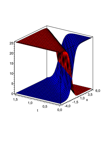
Figure 1: Surfaces representing the components $u$ (blue), $v$ (red) and $w$ (green) of solution (42) with $a=25,\ e=2,\ \alpha=\frac{11}{2}$ of the DLV system (16) with the parameters defined by formulae (41).

Restrictions (41) define the signs of the parameters of (16). Depending on the parameter signs (16) can describe different type of interactions of species. It may also happen that formulae (41) lead to a system, which is not applicable for modeling any interaction. Here we present an example when the exact solution can be useful. It can be noted that the following additional restrictions on parameters $a$ and $e$:

$$a>24,\quad e>1,\quad a(e-1)>8e+\frac{8}{3}$$

lead to negative $b_{i},\ c_{i},\ e_{i}$ in the DLV system (16). Thus, we conclude that the system models competition between three populations and the traveling fronts (42) describe their densities in time and space. Interestingly, the competition predicts extinction of the population $w$ while other two population will survive or die out depending on the sign of the velocity $\alpha$. In Fig. 1, three surfaces are presented for the exact solution (42) for the correctly-specified parameters satisfying the above restrictions. As one concludes from Fig. 1, the solution describes the competition, which leads to the extinction of the populations $u$ and $w$, while the population $v$ dominates as $t\to\infty$.

Finally, we present new traveling waves that describe another type of interaction between three populations (cells, chemicals). Assuming that the $u$ and $v$ species compete for the same resources and $w$ is a predator for the above two species, one arrives at the DLV system

$$\begin{array}[]{l}\lambda_{1}u_{t}=u_{xx}+u(a_{1}-b_{1}u-c_{1}v-e_{1}w),\\ \lambda_{2}v_{t}=v_{xx}+v(a_{2}-b_{2}u-c_{2}v-e_{2}w),\\ \lambda_{3}w_{t}=w_{xx}+w(-a_{3}+b_{3}u+c_{3}v-e_{3}w),\end{array}$$ (43)

where all parameters are positive. The competition-prey-predator model (43) differs essentially from those studied in [27, 28, 29] and can be thought as a generalization of the two-component model (40). Applying the tanh-method, we found the traveling wave solutions of (43) with correctly-specified parameters. Omitting awkward calculations, we present only a result. Thus, the competition-prey-predator model (43) with the parameters

$$\begin{array}[]{l}\lambda_{1}=\frac{2(4+a_{1})}{16-a_{3}},\ \lambda_{2}=\frac{2(4+a_{2})}{16-a_{3}},\ \lambda_{3}=1,\vskip 6.0pt plus 2.0pt minus 2.0pt\\ e_{1}=1,\ e_{2}=1,\ e_{3}=3,\end{array}$$

has traveling wave solutions of the form

$$\begin{array}[]{l}u(t,x)=\frac{(8-a_{2})c_{3}+(24+a_{3})c_{2}}{2(b_{3}c_{2}-b_{2}c_{3})}\left(1+\tanh\left(x+\frac{a_{3}-16}{4}\,t\right)\right),\vskip 6.0pt plus 2.0pt minus 2.0pt\\ v(t,x)=\frac{(a_{2}-8)b_{3}-(24+a_{3})b_{2}}{2(b_{3}c_{2}-b_{2}c_{3})}\left(1+\tanh\left(x+\frac{a_{3}-16}{4}\,t\right)\right),\vskip 6.0pt plus 2.0pt minus 2.0pt\\ w(t,x)=2\left(1+\tanh\left(x+\frac{a_{3}-16}{4}\,t\right)\right)^{2},\end{array}$$

provided the restriction on the parameters $a_{k},\ b_{k}$ and $c_{k}$ ($k=1,2,3$)

$$(24+a_{3})(b_{1}c_{2}-b_{2}c_{1})=(8-a_{1})(b_{2}c_{3}-b_{3}c_{2})+(8-a_{2})(b_{3}c_{1}-b_{1}c_{3})$$

holds.

Obviously, there is an infinity number of parameter sets, which satisfy the above restriction and guarantee that the components $u,\ v$ and $w$ are nonnegative. For instance, setting

$$a_{1}=11,\ a_{2}=9,\ a_{3}=4,\ b_{1}=\frac{1}{2},\ b_{2}=\frac{1}{6},\ b_{3}=5,\ c_{1}=6,\ c_{2}=2,\ c_{3}=7,$$

one obtains $\lambda_{1}=\frac{5}{2}$ and $\lambda_{2}=\frac{13}{6}$ and the exact solution

$$\begin{array}[]{l}u(t,x)=\frac{147}{53}\left(1+\tanh\left(x-3\,t\right)\right),\vskip 6.0pt plus 2.0pt minus 2.0pt\\ v(t,x)=\frac{1}{53}\left(1+\tanh\left(x-3\,t\right)\right),\vskip 6.0pt plus 2.0pt minus 2.0pt\\ w(t,x)=2\left(1+\tanh\left(x-3\,t\right)\right)^{2}.\end{array}$$

Notably, this solution predicts that all species die out as $t\to\infty$.

5 Conditional symmetries of the DLV systems

Now we turn to analysis of $Q$-conditional symmetries of the DLV systems. It will be demonstrated that application of such symmetries for solving the DLV systems is more efficient in comparison with the Lie symmetries. First of all we note that (6) is a system of evolution equations. It is well-known that the problem of constructing its $Q$-conditional symmetries for systems of evolution equations essentially depends on the function $\xi^{0}$ in (9) (see, e.g., [33]). Thus, one should consider two different cases :

1. $\xi^{0}\neq 0.$

2. $\xi^{0}=0,\ \xi^{1}\neq 0.$

In Case 1, one may set $\xi^{0}=1$ without loss of generality applying the well-known property of $Q$-conditional symmetry operators (see, e.g., Section 1.2 in [50]). Moreover, in this case the differential consequences of equations $Q(u^{i})=0$ (that are presented in the manifold ${\cal{M}}_{m}$) w.r.t. the independent variables $t$ and $x$ lead to second-order PDEs involving the derivatives $u^{i}_{tt}$ and the mixed derivatives $u^{i}_{tx}$. However, $u^{i}_{tt}$ and $u^{i}_{tx}$ do not occur in the invariance conditions (11). Thus, the manifold ${\cal{M}}_{m}$ can be rewritten as $\{S_{i}=0,Q(u^{i})=0,i=1,\ldots,m\}$, i.e. the first-order differential consequences can be omitted.

It is well-known that the task of constructing the $Q$-conditional symmetries in Case 2 ($\xi^{0}=0$) for scalar evolution equations is equivalent to solving the equation in question [53]. This statement can be extended on evolution systems of PDEs. In other words, it means that application of the invariance criteria (11) to operator (9) with $\xi^{0}=0$ after cumbersome calculations leads to a system of DEs, which is equivalent to (6). So, in the case of nonlinear and nonintegrable equations (systems), one can identify only some particular cases of the $Q$-conditional symmetry operators of the form (9) with $\xi^{0}=0$. In [33], the two-component DLV system (4) was examined in order to find $Q$-conditional symmetries in Case 2 (the so-called no-go case) using Definition 3.

The system of DEs for finding $Q$-conditional symmetries of the DLV system (13) for the first time was derived in [32]. An algorithm based on Definition 2 was applied for this purpose. In particular, it was shown that the structure of any $Q$-conditional symmetry of (13) can be specified as follows

$$Q=\partial_{t}+\xi\partial_{x}+\left(q^{1}v+r^{1}u+p^{1}\right)\partial_{u}+\left(q^{2}u+r^{2}v+p^{2}\right)\partial_{v},$$ (44)

where the functions $q^{k}(t,x),\ r^{k}(t,x)$ and $p^{k}(t,x)\ (k=1,2)$ should be found from the remaining equations of the system of DEs (see equations (30)–(45) in [32]). The system is very complicated and was not completely integrated, however important results were derived. In particular, the following existence theorem was proved.

Theorem 4

[32] In the case $\lambda_{1}=\lambda_{2}$, DLV system (13) admits only such $Q$-conditional operators of the form (44), which are equivalent to the Lie symmetry operators. In the case $\lambda_{1}\neq\lambda_{2}$, DLV system (13) is $Q$-conditionally invariant under operator (44) if and only if $b_{1}=b_{2}=b$ and $c_{1}=c_{2}=c.$

In order to find symmetries in explicit forms, the case $\lambda_{1}\neq\lambda_{2}$ was examined. As a result, the following theorem was proved.

Theorem 5

[32] If $bc=0,\ b^{2}+c^{2}\neq 0$ then system (13) and the $Q$-conditional symmetries (up to the transformations $u\rightarrow bu,\ v\rightarrow\exp\left(\frac{a_{2}}{\lambda_{2}}t\right)v,\ b\neq 0$ and $u\rightarrow\exp\left(\frac{a_{1}}{\lambda_{1}}t\right)v,\ cv\rightarrow u,$ $c\neq 0$) have the forms

$$\begin{array}[]{l}\lambda_{1}u_{t}=u_{xx}+u(a_{1}+u),\\ \lambda_{2}v_{t}=v_{xx}+vu,\vskip 6.0pt plus 2.0pt minus 2.0pt\\ Q=\partial_{t}+\frac{2\alpha_{1}}{\lambda_{1}-\lambda_{2}}\,\partial_{x}+\left(\varphi(t)\exp(\alpha_{1}x)u+\exp(\alpha_{1}x)\left(\lambda_{2}\varphi^{\prime}(t)+a_{1}\varphi(t)-\alpha^{2}_{1}\varphi(t)\right)+\alpha_{2}v\right)\partial_{v},\end{array}$$

where the function $\varphi(t)\neq 0$ is the general solution of the linear ODE

$$\lambda^{2}_{2}\varphi^{\prime\prime}+\lambda_{2}(a_{1}-2\alpha^{2}_{1})\varphi^{\prime}+\alpha^{2}_{1}(\alpha^{2}_{1}-a_{1})\varphi=0.$$

If $bc\neq 0$ and the additional restrictions

$$q^{1}_{x}=q^{2}_{x}=0$$ (45)

hold then exactly three cases (up to the transformations $u\rightarrow bu,\ v\rightarrow cv$ and $u\rightarrow v,\ v\rightarrow u$) exist when system (13) is invariant w.r.t. $Q$-conditional symmetry operators. These cases are listed in Table 3

Table 3: $Q$-conditional symmetries of the DLV system (13) with $\lambda_{1}\neq\lambda_{2}$ and $b_{1}=b_{2}=b,\ c_{1}=c_{2}=c,\ bc\neq 0$.

	DLV systems	Restrictions	Operators
1	$\lambda_{1}u_{t}=u_{xx}+u(a_{1}+u+v)$	$a_{1}\neq a_{2}$	$(\lambda_{1}-\lambda_{2})\partial_{t}-(a_{1}v+a_{2}u+a_{1}a_{2})(\partial_{u}-\partial_{v}),\ a_{1}a_{2}\neq 0;$
	$\lambda_{2}v_{t}=v_{xx}+v(a_{2}+u+v)$		$(\lambda_{1}-\lambda_{2})\partial_{t}+(a_{1}-a_{2})u(\partial_{u}-\partial_{v});$
			$(\lambda_{1}-\lambda_{2})\partial_{t}-(a_{1}-a_{2})v(\partial_{u}-\partial_{v})$
2	$\lambda_{1}u_{t}=u_{xx}+u(a+u+v)$		$(\lambda_{1}-\lambda_{2})\partial_{t}-a(v+u+a)(\partial_{u}-\partial_{v}),\ a\neq 0;$
	$\lambda_{2}v_{t}=v_{xx}+v(a+u+v)$		$(\lambda_{1}-\lambda_{2})t\partial_{t}-(\lambda_{1}v+\lambda_{2}u)(\partial_{u}-\partial_{v})$
3	$\lambda_{1}u_{t}=u_{xx}+u(a\lambda_{1}+u+v)$	$a\neq 0$	$(\lambda_{1}-\lambda_{2})\partial_{t}-a(\lambda_{1}v+\lambda_{2}u+a\lambda_{1}\lambda_{2})(\partial_{u}-\partial_{v});$
	$\lambda_{2}v_{t}=v_{xx}+v(a\lambda_{2}+u+v)$		$\partial_{t}+au(\partial_{u}-\partial_{v});\ \partial_{t}-av(\partial_{u}-\partial_{v});$
			$\partial_{t}+\frac{a\alpha(\lambda_{1}v+\lambda_{2}u+a\lambda_{1}\lambda_{2})}{(e^{-at}-\alpha(\lambda_{1}-\lambda_{2}))}\,(\partial_{u}-\partial_{v}),\alpha\neq 0$

Remark 1

In contrast to Definition 2, applying Definition 3 leads to a complete description (i.e. without additional restrictions) of $Q$-conditional symmetries of the first type (with $\xi^{0}\neq 0$) of the DLV system (13) (see Theorem 2 [32]). Unfortunately all the $Q$-conditional symmetries of the first type, which have been derived, coincide with those listed in Table 3.

Now we turn to Case 2, i.e. the no-go case ($\xi^{0}=0$, see operator (9)), which was was investigated in [33]. As mentioned above, the algorithm based on Definition 2 leads to an unsolvable system of DEs in this case. So, we used Definition 3 in order to find all possible $Q$-conditional symmetries of the first type. The main result can be formulated as follows.

Theorem 6

[33] The DLV system (13) with restrictions (14) is invariant under $Q$-conditional symmetry operator(s) of the first type

$$Q=\ \xi(t,x,u,v)\partial_{x}+\eta^{1}(t,x,u,v)\partial_{u}+\eta^{2}(t,x,u,v)\partial_{v},\ \xi\neq 0,$$ (46)

if and only if the system and the relevant operator(s) are as specified in Table 4. Any other DLV system (13) admitting a $Q$-conditional symmetry of the first type and the corresponding operator(s) are reducible to those listed in Table 4 by an appropriate transformation from the set

$$t^{*}=t+t_{0},\ x^{*}=e^{\gamma_{0}}(x+x_{0}),\ u^{*}=\beta_{11}\,e^{\gamma_{1}t}u+\beta_{12}\,v,\ v^{*}=\beta_{22}\,e^{\gamma_{2}t}v+\beta_{21}\,u,$$

where $t_{0},\ x_{0},\ \beta_{ij}$ and $\gamma_{j}$ are correctly-specified constants.

Table 4: $Q$-conditional symmetries of the first type of the DLV system (13)

	DLV systems	Restrictions	Operators
1	$\lambda_{1}u_{t}=u_{xx}+u(a_{1}+u+v)$	$\lambda_{1}\neq\lambda_{2}$	$Q^{u}_{1}=\partial_{x}+\frac{g^{1}_{x}}{g^{1}}\,u\,(\partial_{u}-\partial_{v}),$
	$\lambda_{2}v_{t}=v_{xx}+v(a_{2}+\frac{\lambda_{2}}{\lambda_{1}}\,u+\frac{\lambda_{2}}{\lambda_{1}}\,v)$		$Q^{v}_{1}=\partial_{x}+\frac{g^{2}_{x}}{g^{2}}\,v\,(\partial_{v}-\partial_{u})$
2	$u_{t}=u_{xx}+u(a+u+2v)$		$Q^{v}_{2}=G(x,v)\left(\partial_{x}+F(x,v)(\partial_{u}-\partial_{v})\right)$
	$\lambda v_{t}=v_{xx}+v(a+v)$
3	$u_{t}=u_{xx}+uv$	$a_{2}c_{2}\neq 0$	$Q^{u}_{3}=\partial_{x}+r(t,x)\,u\,\partial_{u},$
	$\lambda v_{t}=v_{xx}+v(a_{2}+c_{2}v)$		$Q^{v}_{3}=\left(h^{1}(\omega)-2th^{2}(\omega)\right)\partial_{x}$
			$+\left((h^{2}(\omega)x+h^{3}(\omega))u+p(t,x,v)\right)\partial_{u}$
4	$u_{t}=u_{xx}+uv$	$c_{2}\neq 0$	$Q^{u}_{3},\ Q^{v}_{4}=\left(h^{1}(\theta)-2th^{2}(\theta)\right)\partial_{x}$
	$\lambda v_{t}=v_{xx}+c_{2}v^{2}$		$+\left((h^{2}(\theta)x+h^{3}(\theta))u+p(t,x,v)\right)\partial_{u}$
5	$u_{t}=u_{xx}+uv$	$a_{2}\neq 0$	$Q^{u}_{3},\quad Q^{v}_{3},\quad Q^{v}_{5}=\partial_{x}+e^{a_{2}t}u\partial_{v}$
	$v_{t}=v_{xx}+v\left(a_{2}+\frac{v}{2}\right)$		$+\left(\alpha\,u-\frac{e^{-a_{2}t}}{2}\,v^{2}-a_{2}e^{-a_{2}t}v\right)\partial_{u}$
6	$u_{t}=u_{xx}+uv$		$Q^{u}_{3},\ Q^{v}_{4},$
	$v_{t}=v_{xx}+\frac{1}{2}\,v^{2}$		$Q^{v}_{6}=(\alpha_{1}t+\alpha_{0})\partial_{x}+(\alpha_{1}t+\alpha_{0})u\partial_{v}$
			$+\left(\left(\alpha_{2}-\frac{\alpha_{1}}{2}\,x\right)u-\frac{\alpha_{1}t+\alpha_{0}}{2}\,v^{2}-\alpha_{1}v\right)\partial_{u}$
7	$u_{t}=u_{xx}+uv$	$a_{2}\neq 0$	$\alpha_{1}^{2}+\alpha_{2}^{2}\neq 0$,   $Q^{u}_{3},\ Q^{v}_{3},$
	$v_{t}=v_{xx}+v(a_{2}+v)$		$Q^{u}_{7}=\partial_{x}+\left(-\frac{x}{2t}\,u+\frac{\alpha_{1}}{t}\right.$
			$+\left.\left(\frac{\alpha_{2}e^{-a_{2}t}}{t}+\frac{\alpha_{1}}{a_{2}t}\right)v\right)\partial_{u}$
8	$u_{t}=u_{xx}+uv$	$\alpha_{1}^{2}+\alpha_{2}^{2}\neq 0$	$Q^{u}_{3},\ Q^{v}_{4},$
	$v_{t}=v_{xx}+v^{2}$		$Q^{u}_{8}=\partial_{x}+\left(-\frac{x}{2t}\,u+\frac{\alpha_{1}}{t}+\left(\frac{\alpha_{2}}{t}+\alpha_{1}\right)v\right)\partial_{u}$

Remark 2

In Table 4, the upper indices $u$ and $v$ mean that the relevant $Q$-conditional symmetry operators satisfy Definition 3 in the case of the manifold ${\cal{M}}^{1}_{1}$ ($u^{1}=u$) and ${\cal{M}}^{2}_{1}$ ($u^{2}=v$), respectively.

Remark 3

In Table 4, $\omega=\frac{a_{2}+c_{2}v}{\lambda v}\,e^{\frac{a_{2}}{\lambda}\,t},\ \theta=t+\frac{\lambda}{c_{2}v};$ $h^{1},\ h^{2}$ and $h^{3}$ are arbitrary smooth functions of the relevant variables, while the function $p(t,x,v)$ is the general solution of the linear ODE

$$p_{t}=p_{xx}-\frac{v(a_{2}+c_{2}v)}{\lambda}p_{v}+vp,$$

the functions $F$ and $G$ form the general solution of the system

$$FF_{v}-F_{x}+av+v^{2}=0,\ G_{x}=FG_{v},$$

the function $r(t,x)$ is the general solution of the Burgers equation

$$r_{t}=r_{xx}+2rr_{x},$$

while

$$g^{i}(t,x)=\left\{\begin{array}[]{l}\alpha_{0}\exp\left(\frac{\kappa^{2}t}{\lambda_{i}}\right)+\alpha_{1}\sin(\kappa\,x)+\alpha_{2}\cos(\kappa\,x),\quad\mbox{if}\quad\frac{\lambda_{1}a_{2}-\lambda_{2}a_{1}}{\lambda_{1}-\lambda_{2}}>0,\vskip 6.0pt plus 2.0pt minus 2.0pt\\ \alpha_{0}\exp\left(-\frac{\kappa^{2}t}{\lambda_{i}}\right)+\alpha_{1}e^{\kappa x}+\alpha_{2}e^{-\kappa x},\quad\mbox{if}\quad\frac{\lambda_{1}a_{2}-\lambda_{2}a_{1}}{\lambda_{1}-\lambda_{2}}<0,\vskip 6.0pt plus 2.0pt minus 2.0pt\\ \alpha_{0}+\alpha_{1}x+\alpha_{2}\lambda_{i}x^{2}+2\alpha_{2}t,\quad\mbox{if}\quad\lambda_{1}a_{2}=\lambda_{2}a_{1},\end{array}\right.$$ (47)

where $i=1,2,$ $\kappa=\sqrt{\left|\frac{\lambda_{1}a_{2}-\lambda_{2}a_{1}}{\lambda_{1}-\lambda_{2}}\right|},$ $\alpha_{0},\ \alpha_{1}$ and $\alpha_{2}$ are arbitrary constants.

It should be noted that all the systems arising in Table 4, except that in Case 1, are semi-coupled (see the second equation is each system). We point out that the second equation in Cases 2, 3, 5 and 7 is nothing else but the famous Fisher equation. Obviously, Case 1 from Table 4 is the most interesting from applicability point of view. In fact, it will be demonstrated in Section 6 that the system from Case 1 models competition of two populations of species (cells, chemicals) and the relevant exact solutions will be constructed.

Now we turn to the three-component DLV system. A complete description of the $Q$-conditional (nonclassical) symmetry for the three-component DLV system is still unknown from the same reason as for the two-component system. To the best of our knowledge, there is only a single study [34] devoted only to the search for conditional symmetries of the three-component DLV system. In that paper, all possible $Q$-conditional symmetries of the first type were derived in Case 1.

Theorem 7

[34] The DLV system (16) is invariant under $Q$-conditional symmetry of the first type

$$\begin{array}[]{l}Q=\xi^{0}(t,x,u,v,w)\partial_{t}+\xi^{1}(t,x,u,v,w)\partial_{x}+\eta^{1}(t,x,u,v,w)\partial_{u}+\\ \hskip 51.21504pt\eta^{2}(t,x,u,v,w)\partial_{v}+\eta^{3}(t,x,u,v,w)\partial_{w},\ \xi^{0}\neq 0,\end{array}$$

if and only if it and the relevant operators are as specified in Table 5. Any other DLV system admitting a $Q$-conditional symmetry operator of the first type is reduced to one of those from Table 5 by a transformation from the set (18).

Table 5: $Q$-conditional symmetries of the first type of the DLV system (16)

	Reaction terms	Restrictions	$Q$-conditional symmetry operators
1	$u(a_{1}+bu+bv+ew)$	$(b-1)^{2}+(e-e_{3})^{2}\neq 0,$	$\partial_{t}+\frac{a_{1}-a_{2}}{\lambda_{1}-\lambda_{2}}u(\partial_{u}-\partial_{v}),$
	$v(a_{2}+bu+bv+ew)$	$a_{1}\neq a_{2}$	$\partial_{t}+\frac{a_{1}-a_{2}}{\lambda_{1}-\lambda_{2}}v(\partial_{v}-\partial_{u})$
	$w(a_{3}+u+v+e_{3}w)$
2	$u(a_{1}+u+v+w)$	$(a_{1}-a_{2})^{2}+(a_{1}-a_{3})^{2}\neq 0$	$Q^{2}_{i},\ i=1,\dots,6$
	$v(a_{2}+u+v+w)$
	$w(a_{3}+u+v+w)$
3	$u(a_{1}+u+v+w)$	$(\lambda_{2}-\lambda_{3})a_{1}-\lambda_{2}a_{3}$	$Q^{2}_{i},\ i=1,\dots,6,$
	$v(a_{2}+u+v+w)$	$+\lambda_{3}a_{2}=0,$	$\partial_{t}+\beta\exp\left(\frac{a_{2}-a_{3}}{\lambda_{2}-\lambda_{3}}t\right)u(\partial_{v}-\partial_{w})$
	$w(a_{3}+u+v+w)$	$a_{2}\neq a_{3},\ \beta\neq 0$
4	$u(a_{1}+u+v+w)$	$(\lambda_{2}-\lambda_{3})a_{1}-(\lambda_{1}-\lambda_{3})a_{2}$	$Q^{4}_{i},\ i=1,\dots,6$
	$v(a_{2}+u+v+w)$	$+(\lambda_{1}-\lambda_{2})a_{3}=0,$
	$w(a_{3}+u+v+w)$	$(a_{1}-a_{2})^{2}+\alpha^{2}\neq 0$
5	$u(a_{1}+bu+v)$	$(b-1)^{2}+(c-1)^{2}\neq 0$	$Q^{5}_{1}$
	$v(a_{2}+u+cv)$
	$w(bu+v)$
6	$u(a_{1}+u+v)$		$Q^{5}_{1},\ Q^{6}_{i},\ i=1,\dots,4$
	$v(a_{2}+u+v)$
	$w(u+v)$
7	$u(a_{1}+bu+cv)$	$\lambda_{2}=\lambda_{3}=1,\ b\neq 1,\ c\neq 1,$	$\partial_{t}+\left((1-b)u+(1-c)v+a_{2}(1-c)\right)\partial_{w}$
	$v(a_{2}+u+v)$	$a_{1}(1-b)=a_{2}b(1-c)$
	$w(bu+v)$
8	$u(a+bu+cv)$	$\lambda_{2}=\lambda_{3}=1,\ b\neq 1,\ c\neq 1,$	$\partial_{t}+(1-c)\partial_{w}$
	$v(a+u+v)$	$b(2-c)=1$	$+\left((1-b)u+(1-c)v\right)\varphi_{4}(t)\partial_{w}$
	$w(bu+v)$
9	$u(a_{1}+u+v)$	$\lambda_{2}=\lambda_{3}=1$	$Q^{9}_{i},\ i=1,\dots,5$
	$v(a_{2}+u+v)$
	$w(u+v)$

The coefficients $\lambda_{k}>0\ (k=1,2,3)$ are assumed to be different in cases 1–6.

In Table 5, the following designations are introduced:

$$Q^{2}_{i}=Q^{4}_{i}\ \mbox{with}\ \alpha=0,\ i=1,\dots,6;$$

$$Q^{4}_{1}=\partial_{t}+\frac{a_{1}-a_{2}}{\lambda_{1}-\lambda_{2}}u(\partial_{u}-\partial_{v})+\alpha u(\partial_{v}-\partial_{w}),\ Q^{4}_{2}=\partial_{t}+\frac{a_{1}-a_{2}}{\lambda_{1}-\lambda_{2}}v(\partial_{v}-\partial_{u})+\alpha v(\partial_{u}-\partial_{w}),$$

$$Q^{4}_{3}=\partial_{t}+\frac{a_{1}-a_{3}}{\lambda_{1}-\lambda_{3}}u(\partial_{u}-\partial_{w})+\alpha u(\partial_{v}-\partial_{w}),\ Q^{4}_{4}=\partial_{t}+\frac{a_{1}-a_{3}}{\lambda_{1}-\lambda_{3}}w(\partial_{w}-\partial_{u})+\alpha w(\partial_{u}-\partial_{v}),$$

$$Q^{4}_{5}=\partial_{t}+\frac{a_{2}-a_{3}}{\lambda_{2}-\lambda_{3}}v(\partial_{v}-\partial_{w})+\alpha v(\partial_{u}-\partial_{w}),\ Q^{4}_{6}=\partial_{t}+\frac{a_{2}-a_{3}}{\lambda_{2}-\lambda_{3}}w(\partial_{w}-\partial_{v})+\alpha w(\partial_{u}-\partial_{v});$$

$$Q^{5}_{1}=\partial_{t}+\alpha_{1}\partial_{x}+\exp\left(\left(\frac{(\lambda_{1}-\lambda_{3})^{2}}{4}\alpha^{2}_{1}-a_{1}\right)\frac{t}{\lambda_{3}}+\frac{\lambda_{1}-\lambda_{3}}{2}\alpha_{1}x\right)u\partial_{w};$$

$$Q^{6}_{1}=\partial_{t}+\alpha_{1}\partial_{x}+\exp\left(\left(\frac{(\lambda_{2}-\lambda_{3})^{2}}{4}\alpha^{2}_{1}-a_{2}\right)\frac{t}{\lambda_{3}}+\frac{\lambda_{2}-\lambda_{3}}{2}\alpha_{1}x\right)v\partial_{w},$$

$$Q^{6}_{2}=\partial_{t}+\frac{a_{1}-a_{2}}{\lambda_{1}-\lambda_{2}}u(\partial_{u}-\partial_{v})+\beta\exp\left(\frac{(\lambda_{1}-\lambda_{3})a_{2}-(\lambda_{2}-\lambda_{3})a_{1}}{\lambda_{3}(\lambda_{2}-\lambda_{1})}t\right)u\partial_{w},$$

$$Q^{6}_{3}=\partial_{t}+\frac{a_{1}-a_{2}}{\lambda_{1}-\lambda_{2}}v(\partial_{v}-\partial_{u})+\beta\exp\left(\frac{(\lambda_{2}-\lambda_{3})a_{1}-(\lambda_{1}-\lambda_{3})a_{2}}{\lambda_{3}(\lambda_{1}-\lambda_{2})}t\right)v\partial_{w},$$

$$Q^{6}_{4}=\partial_{t}+\frac{a_{2}\lambda_{1}-a_{1}\lambda_{2}}{\lambda_{3}(\lambda_{2}-\lambda_{1})}w\partial_{w}+\exp\left(\frac{(\lambda_{3}-\lambda_{2})a_{1}-(\lambda_{3}-\lambda_{1})a_{2}}{\lambda_{3}(\lambda_{1}-\lambda_{2})}t\right)w(\partial_{u}-\partial_{v});$$

$$Q^{9}_{1}=Q^{5}_{1}\ \mbox{with}\ \lambda_{3}=1,\quad Q^{9}_{2}=Q^{6}_{4}\ \mbox{with}\ \lambda_{2}=\lambda_{3}=1,$$

$$Q^{9}_{3}=\partial_{t}+\frac{a_{1}-a_{2}}{\lambda_{1}-1}u(\partial_{u}-\partial_{v})+\left(\varphi_{1}(t)u+\varphi_{2}(t)v+\beta_{1}\right)\partial_{w},$$

$$Q^{9}_{4}=\partial_{t}+\left(\varphi_{3}(t)u+\varphi_{2}(t)v+\beta_{1}\right)\partial_{w},\quad Q^{9}_{5}=\partial_{t}+\frac{a_{1}-a_{2}}{\lambda_{1}-1}v(\partial_{v}-\partial_{u});$$

where the functions $\varphi_{i}(t)\ (i=1,\dots,4)$ are as follows:

$$\varphi_{1}(t)=\left\{\begin{array}[]{l}\beta_{1}t+\beta_{2},\ \mbox{if}\ a_{2}=0,\\ \beta_{2}\exp(-a_{2}t)+\frac{\beta_{1}}{a_{2}},\ \mbox{if}\ a_{2}\neq 0,\end{array}\right.\quad\varphi_{2}(t)=\left\{\begin{array}[]{l}\beta_{1}t,\ \mbox{if}\ a_{2}=0,\\ \frac{\beta_{1}}{a_{2}},\ \mbox{if}\ a_{2}\neq 0,\end{array}\right.$$

$$\varphi_{3}(t)=\left\{\begin{array}[]{l}\beta_{1}t+\beta_{2},\ \mbox{if}\ a_{1}=0,\\ \beta_{2}\exp(-a_{1}t)+\frac{\beta_{1}}{a_{1}},\ \mbox{if}\ a_{1}\neq 0,\end{array}\right.\quad\varphi_{4}(t)=\left\{\begin{array}[]{l}t+\beta,\ \mbox{if}\ a=0,\\ \beta\exp(-at)+\frac{1}{a},\ \mbox{if}\ a\neq 0,\end{array}\right.$$

while $\alpha$ and $\beta$ (with and without subscripts 1 and 2) are arbitrary constants.

Remark 4

The inequalities listed in the third column of Table 5 guarantee that the $Q$-conditional symmetries from the fourth column are not equivalent to any Lie symmetry presented in Table 2.

We conclude that the three-component DLV system, depending on the coefficient restrictions, admits a wider range of $Q$-conditional symmetries of the first type compared to those for the two-component DLV system. In particular, there are cases when DLV system (16) admits sets consisting of 5, 6 and even 7 different symmetries. All these symmetries can be successfully used for finding exact solutions.

From the applicability point of view, the systems arising in cases 1–4 of Table 5 are most promising because their nonzero coefficients do not affect the biological sense of these systems. In the Section 7, we examine these systems.

Concluding this section, we present a short statement about the $m$-component DLV system (9). In the case of the DLV system (9) with $m>3$, the problem of constructing conditional symmetries is still open. Some particular results can be obtained by a simple generalization of the results obtained for three-component system. In particular, we proved that the $m$-component system [34]

$$\lambda_{i}u^{i}_{t}=u^{i}_{xx}+u^{i}(a_{i}+u^{1}+\dots+u^{m}),\ i=1,2,\dots,m$$

admits $m(m-1)$ operators of the form

$$Q_{ij}=\partial_{t}+\frac{a_{i}-a_{j}}{\lambda_{i}-\lambda_{j}}u^{i}\left(\partial_{u^{i}}-\partial_{u^{j}}\right),\ \ i\not=j=1,2,\dots,m,$$

provided $(a_{i}-a_{j})(\lambda_{i}-\lambda_{j})\not=0$. One may consider the above system and the operators as a generalization of those presented in Case 2 of Table 5 on the case of the $m$-component DLV systems.

6 Exact solutions of the two-component DLV system

This section is devoted to the construction of exact solutions with more complicated structures than the traveling wave solutions presented in Section 4. It should be pointed out that the traveling wave solutions cannot be applied for solving practical models, in particular based on the DLV systems, describing processes in bounded domains. In fact, any traveling front does not satisfy typical boundary conditions like no-flux conditions or/and constant densities at a bounded interval. It means that an ansatz of the form (8) should be used for search for exact solutions.

It is well-known that using $Q$-conditional symmetries a given two-dimensional PDE (system of PDEs) can be reduced to an ODE (system of ODEs) via the same algorithm as for classical Lie symmetries. It means that the ansatz corresponding to the given operator $Q$ can be constructed provided the linear (quasi-linear) first-order PDEs

$${Q}(u)=0,\ {Q}(v)=0$$ (48)

are solved.

Theorems 5 and 6 give several possibilities for finding exact solutions of the DLV system with correctly-specified coefficients.

Let us consider the DLV system from Case 1 of Table 3, namely :

$$\begin{array}[]{l}\lambda_{1}u_{t}=u_{xx}+u(a_{1}+u+v),\\ \lambda_{2}v_{t}=v_{xx}+v(a_{2}+u+v),\ a_{1}\neq a_{2},\end{array}$$ (49)

and its $Q$-conditional symmetry operator

$$Q=(\lambda_{1}-\lambda_{2})\partial_{t}-(a_{1}v+a_{2}u+a_{1}a_{2})(\partial_{u}-\partial_{v}).$$ (50)

In the case of operator (50), system (48) takes the form

$$\begin{array}[]{l}(\lambda_{1}-\lambda_{2})u_{t}=-(a_{1}v+a_{2}u+a_{1}a_{2}),\\ (\lambda_{1}-\lambda_{2})v_{t}=a_{1}v+a_{2}u+a_{1}a_{2}.\end{array}$$ (51)

It follows immediately from (51) that $u_{t}=-v_{t}$, hence

$$u(t,x)=-v(t,x)+\varphi_{1}(x).$$ (52)

Substituting (52) into the second equation of (51), one obtains the linear equation

$$(\lambda_{1}-\lambda_{2})v_{t}=(a_{1}-a_{2})v+a_{2}\varphi_{1}(x)+a_{1}a_{2}.$$

Since $a_{1}\neq a_{2}$ this equation has the general solution

$$v=\frac{1}{a_{1}-a_{2}}\left(\exp\left(\frac{a_{1}-a_{2}}{\lambda_{1}-\lambda_{2}}t\right)\varphi_{2}(x)-a_{2}\varphi_{1}(x)-a_{1}a_{2}\right),$$

therefore the ansatz

$$\begin{array}[]{l}u=\frac{1}{a_{1}-a_{2}}\left(-\exp\left(\frac{a_{1}-a_{2}}{\lambda_{1}-\lambda_{2}}t\right)\varphi_{2}(x)+a_{1}\varphi_{1}(x)+a_{1}a_{2}\right),\\ v=\frac{1}{a_{1}-a_{2}}\left(\exp\left(\frac{a_{1}-a_{2}}{\lambda_{1}-\lambda_{2}}t\right)\varphi_{2}(x)-a_{2}\varphi_{1}(x)-a_{1}a_{2}\right)\end{array}$$ (53)

is obtained. Here $\varphi_{1}$ and $\varphi_{2}$ are functions to be found.

To obtain the reduced system, we substitute ansatz (53) into (49). This means that we simply calculate the derivatives $u_{t},\ v_{t},\ u_{xx},\ v_{xx},$ and insert them into (49). Making relevant calculations, one arrives at the ODE system

$$\begin{array}[]{l}\varphi^{\prime\prime}_{1}+\varphi^{2}_{1}+(a_{1}+a_{2})\varphi_{1}+a_{1}a_{2}=0,\\ \varphi^{\prime\prime}_{2}+\frac{a_{2}\lambda_{1}-a_{1}\lambda_{2}}{\lambda_{1}-\lambda_{2}}\,\varphi_{2}+\varphi_{1}\varphi_{2}=0\end{array}$$ (54)

to find the functions $\varphi_{1}$ and $\varphi_{2}$.

Remark 5

Using the second and third operators listed in Case 1 of Table 3, one can obtain reduced systems in a similar way and look for exact solutions. However, we have checked that the ODE systems obtained simply follow from (54) by removing the terms $a_{1}\varphi_{1}+a_{1}a_{2}$.

In order to construct exact solutions, now we examine the ODE systems obtained above. To the best of our knowledge, the general solution of the nonlinear ODE system (54) is unknown, therefore we look for its particular solutions. Setting $\varphi_{1}=\alpha=const,$ we conclude

$$\alpha^{2}+(a_{1}+a_{2})\alpha+a_{1}a_{2}=0\ \Rightarrow\ \alpha_{1}=-a_{1},\ \alpha_{2}=-a_{2}$$

from the first equation of system (54). So, setting $\varphi_{1}=-a_{1}$ (the case $\varphi_{1}=-a_{2}$ leads to the solution with the same structure) and substituting into the second equation of system (54), we obtain the linear ODE:

$$\varphi^{\prime\prime}_{2}-\beta\lambda_{1}\varphi_{2}=0,$$ (55)

where $\beta=\frac{a_{1}-a_{2}}{\lambda_{1}-\lambda_{2}}\not=0.$ Depending on the sign of the parameter $\beta$ the linear ODE (55) possesses two families of general solutions. These solutions and ansatz (53) lead to the following exact solutions of the DLV system (49):

$$\begin{array}[]{l}u=-a_{1}+\frac{1}{a_{2}-a_{1}}\left(C_{1}\exp\left(\sqrt{\beta\lambda_{1}}x\right)+C_{2}\exp\left(-\sqrt{\beta\lambda_{1}}x\right)\right)e^{\beta t},\\ v=\frac{1}{a_{1}-a_{2}}\left(C_{1}\exp\left(\sqrt{\beta\lambda_{1}}x\right)+C_{2}\exp\left(-\sqrt{\beta\lambda_{1}}x\right)\right)e^{\beta t},\end{array}$$

if $\beta>0,$ and

$$\begin{array}[]{l}u=-a_{1}+\frac{1}{a_{2}-a_{1}}\left(C_{1}\cos\left(\sqrt{-\beta\lambda_{1}}x\right)+C_{2}\sin\left(\sqrt{-\beta\lambda_{1}}x\right)\right)e^{\beta t},\\ v=\frac{1}{a_{1}-a_{2}}\left(C_{1}\cos\left(\sqrt{-\beta\lambda_{1}}x\right)+C_{2}\sin\left(\sqrt{-\beta\lambda_{1}}x\right)\right)e^{\beta t},\end{array}$$ (56)

if $\beta<0$ (hereinafter $C_{1}$ and $C_{2}$ are arbitrary constants).

Now we demonstrate that extra exact solutions of (54) can be derived provided some restrictions on $\lambda_{1}$ and $\lambda_{2}$ take place. Indeed, we note that the substitution

$$\varphi_{1}=\varphi-a_{1}$$ (57)

simplifies the first equation of (54) to the form

$$\varphi^{\prime\prime}+\varphi^{2}+(a_{2}-a_{1})\varphi=0.$$ (58)

Of course, (58) can be reduced to the first-order ODE

$$\left(\frac{d\varphi}{dx}\right)^{2}=-\frac{2}{3}\ \varphi^{3}+(a_{1}-a_{2})\varphi^{2}+C\$$

with the general solution involving the Weierstrass function [54]. Now we set $C=0$ in order to avoid cumbersome formulae, therefore the general solution is

$$\varphi=\frac{3(a_{1}-a_{2})}{2}\left(1-\tanh^{2}\left(\frac{\sqrt{a_{1}-a_{2}}}{2}\,x\right)\right),$$ (59)

if $a_{1}>a_{2}$, and

$$\varphi=\frac{3(a_{1}-a_{2})}{2}\left(1+\tan^{2}\left(\frac{\sqrt{a_{2}-a_{1}}}{2}\,x\right)\right),$$ (60)

if $a_{1}<a_{2}.$

Thus, we can apply formulae (59) and (60) to solve the second ODE of (54). In the case of solution (59), this ODE takes the form

$$\varphi_{2}^{\prime\prime}+\varphi_{2}(a_{1}-a_{2})\left(\frac{\lambda_{1}-3\lambda_{2}}{2(\lambda_{1}-\lambda_{2})}-\frac{3}{2}\tanh^{2}\left(\frac{\sqrt{a_{1}-a_{2}}}{2}\,x\right)\right)=0.$$ (61)

The general solution of (61) with some restrictions on $\lambda_{1}$ and $\lambda_{2}$ can be found [55]:

$$\varphi_{2}=f_{1}(x)\left(C_{1}+C_{2}\int\frac{1}{f^{2}_{1}(x)}\,dx\right),$$ (62)

if $\lambda_{1}=\frac{9}{5}\lambda_{2}$, and

$$\varphi_{2}=f_{2}(x)\left(C_{1}+C_{2}\int\frac{1}{f^{2}_{2}(x)}\,dx\right),$$ (63)

if $\lambda_{1}=\frac{4}{3}\lambda_{2}$, where

$$f_{1}(x)=\cosh^{3}\left(\frac{\sqrt{a_{1}-a_{2}}}{2}\,x\right),\quad f_{2}(x)=\sinh\left(\frac{\sqrt{a_{1}-a_{2}}}{2}\,x\right)\cosh^{3}\left(\frac{\sqrt{a_{1}-a_{2}}}{2}\,x\right).$$

Thus, substituting the functions $\varphi_{1}(x)$ and $\varphi_{2}(x)$ given by formulae (57), (59) and (62) into ansatz (53), one easily obtain exact solutions of the DLV system (49) (see [32] for details).

Let us consider an example.

Example 1. Using the substitution

$$u\rightarrow-bu,\ v\rightarrow-cv\ (b>0,\ c>0),$$

one reduces the DLV system (49) to the system

$$\begin{array}[]{l}\lambda_{1}u_{t}=u_{xx}+u(a_{1}-bu-cv),\\ \lambda_{2}v_{t}=v_{xx}+v(a_{2}-bu-cv),\end{array}$$ (64)

which describes competition of two species (here $a_{1}>0,a_{2}>0$ and $\lambda_{1}\not=\lambda_{2}$). Simultaneously this substitution transforms solution (56) with $C_{1}=0$ to the form

$$\begin{array}[]{l}u(t,x)=\frac{a_{1}}{b}+\frac{1}{(a_{1}-a_{2})b}\ C_{2}\sin\left(\sqrt{-\beta\lambda_{1}}x\right)e^{\beta t},\\ v(t,x)=\frac{1}{(a_{2}-a_{1})c}\ C_{2}\sin\left(\sqrt{-\beta\lambda_{1}}x\right)e^{\beta t},\end{array}$$ (65)

where the coefficient restrictions $\beta\equiv\frac{a_{1}-a_{2}}{\lambda_{1}-\lambda_{2}}<0,\ a_{1}>0,\ a_{2}>0$ are assumed. Having this solution, we formulate the following theorem about the classical solution of a nonlinear BVP involving constant Dirichlet conditions.

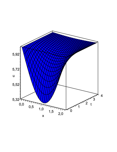
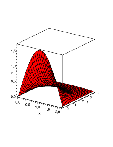
Figure 2: Surfaces representing the $u$ (blue) and $v$ (red) components of solution (65) with $C_{2}=\frac{1}{3},\ \beta=-1$ of system (64) with the parameters $a_{1}=3,\ a_{2}=4,\ b=\frac{1}{2},\ c=\frac{1}{5},\ \lambda_{1}=2,\ \lambda_{2}=1.$

Theorem 8

[32] The classical solution of the nonlinear BVP formed by the competition system (64), the initial profile

$$\begin{array}[]{l}u(0,x)=\frac{a_{1}}{b}+\frac{1}{(a_{1}-a_{2})b}\ C_{2}\sin\left(\sqrt{-\beta\lambda_{1}}x\right),\\ v(0,x)=\frac{1}{(a_{2}-a_{1})c}\ C_{2}\sin\left(\sqrt{-\beta\lambda_{1}}x\right)\end{array}$$

and the boundary conditions

$$\begin{array}[]{l}x=0:\ u=\frac{a_{1}}{b},\ v=0,\\ x=\frac{\pi}{\sqrt{-\beta\lambda_{1}}}:\ u=\frac{a_{1}}{b},\ v=0\end{array}$$

in the domain $\Omega=\left\{(t,x)\in(0,+\infty)\times\Bigl{(}0,\frac{\pi}{\sqrt{-\beta\lambda_{1}}}\Bigr{)}\right\}$ is given by formulae (65).

The solution (65) with $\beta<0$ has the time asymptotic

$$\left(u,\ v\right)\rightarrow\left(\frac{a_{1}}{b},\ 0\right),\quad t\rightarrow+\infty.$$

Using biological terminology, this solution simulates competition between two populations of species when species $u$ eventually dominates while species $v$ dies out. An example of this competition with correctly-specified parameters is shown in Fig. 2.

Now let us consider the DLV system from Case 1 of Table 4, namely :

$$\begin{array}[]{l}\lambda_{1}u_{t}=u_{xx}+u(a_{1}+u+v),\\ \lambda_{2}v_{t}=v_{xx}+v\left(a_{2}+\frac{\lambda_{2}}{\lambda_{1}}u+\frac{\lambda_{2}}{\lambda_{1}}v\right),\ \lambda_{1}\neq\lambda_{2}.\end{array}$$ (66)

It should be noted that the $Q$-conditional symmetry operators $Q^{u}_{1}$ and $Q^{v}_{1}$ of system (66) lead to the same exact solutions (up to discrete transformation $u\rightarrow v,\ v\rightarrow u$). Thus, we use only the operator $Q^{u}_{1}$. The corresponding ansatz can be constructed by solving the linear first-order PDE system

$$u_{x}=\frac{g^{1}_{x}}{g^{1}}\,u,\ v_{x}=-\frac{g^{1}_{x}}{g^{1}}\,u.$$ (67)

Integrating system (67) for each form of the function $g^{1}$ from (47), we obtain the ansatz

$$\begin{array}[]{l}u=\varphi(t)\left(\alpha_{0}+\alpha_{1}\exp\left(-\frac{\kappa^{2}}{\lambda_{1}}\,t\right)\sin(\kappa x)+\alpha_{2}\exp\left(-\frac{\kappa^{2}}{\lambda_{1}}\,t\right)\cos(\kappa x)\right),\\ v=\psi(t)-\varphi(t)\left(\alpha_{0}+\alpha_{1}\exp\left(-\frac{\kappa^{2}}{\lambda_{1}}\,t\right)\sin(\kappa x)+\alpha_{2}\exp\left(-\frac{\kappa^{2}}{\lambda_{1}}\,t\right)\cos(\kappa x)\right),\end{array}$$ (68)

if $\frac{\lambda_{1}a_{2}-\lambda_{2}a_{1}}{\lambda_{1}-\lambda_{2}}>0,$ the ansatz

$$\begin{array}[]{l}u=\varphi(t)\left(\alpha_{0}+\alpha_{1}\exp\left(\frac{\kappa^{2}}{\lambda_{1}}\,t+\kappa x\right)+\alpha_{2}\exp\left(\frac{\kappa^{2}}{\lambda_{1}}\,t-\kappa x\right)\right),\\ v=\psi(t)-\varphi(t)\left(\alpha_{0}+\alpha_{1}\exp\left(\frac{\kappa^{2}}{\lambda_{1}}\,t+\kappa x\right)+\alpha_{2}\exp\left(\frac{\kappa^{2}}{\lambda_{1}}\,t-\kappa x\right)\right),\end{array}$$ (69)

if $\frac{\lambda_{1}a_{2}-\lambda_{2}a_{1}}{\lambda_{1}-\lambda_{2}}<0,$ and the ansatz

$$\begin{array}[]{l}u=\varphi(t)\left(\alpha_{0}+\alpha_{1}x+\alpha_{2}x^{2}+2d_{1}\alpha_{2}t\right),\\ v=\psi(t)-\varphi(t)\left(\alpha_{0}+\alpha_{1}x+\alpha_{2}x^{2}+2d_{1}\alpha_{2}t\right),\end{array}$$ (70)

if $a_{2}=\frac{a_{1}\lambda_{2}}{\lambda_{1}}.$

Now three reductions of the given DLV system to ODE systems can be obtained. In fact, inserting the above ansätze into the DLV system (66), we arrive at the ODE system

$$\lambda_{1}\frac{d\varphi}{dt}=\varphi\left(a_{1}+\psi\right),\ \lambda_{2}\frac{d\psi}{dt}=\left(a_{2}+\frac{\lambda_{2}}{\lambda_{1}}\,\psi\right)\psi+\alpha_{0}\left(\frac{a_{1}\lambda_{2}}{\lambda_{1}}-a_{2}\right)\,\varphi,$$ (71)

in the cases of formulae (68) and (69), while the system

$$\lambda_{1}\frac{d\varphi}{dt}=\varphi\left(a_{1}+\psi\right),\ \lambda_{2}\frac{d\psi}{dt}=\frac{\lambda_{2}}{\lambda_{1}}\left(a_{1}+\psi\right)\psi-2\alpha_{2}\left(\lambda_{1}-\lambda_{2}\right)\,\varphi,$$ (72)

is obtained in the case of (70). Here $\varphi(t)$ and $\psi(t)$ are to-be-determined functions.

It was proved that each of the ODE systems (71) and (72) can be integrated by reducing to a single second-order ODE (see [33] for details). Here we present exact solutions of the DLV system (66) with $a_{1}a_{2}\neq 0$ and $\frac{\lambda_{1}a_{2}-\lambda_{2}a_{1}}{\lambda_{1}-\lambda_{2}}>0$, namely:

$$\begin{array}[]{l}u(t,x)=\frac{a_{1}\exp\left(\frac{a_{1}}{\lambda_{1}}\,t\right)}{C_{1}-\alpha_{0}\exp\left(\frac{a_{1}}{\lambda_{1}}\,t\right)+C_{2}\lambda_{2}\exp\left(\frac{a_{2}}{\lambda_{2}}\,t\right)}\left(\alpha_{0}+\alpha_{1}\exp\left(-\frac{\kappa^{2}}{\lambda_{1}}\,t\right)\sin(\kappa x)+\alpha_{2}\exp\left(-\frac{\kappa^{2}}{\lambda_{1}}\,t\right)\cos(\kappa x)\right),\vskip 6.0pt plus 2.0pt minus 2.0pt\\ v(t,x)=\frac{\alpha_{0}a_{1}\exp\left(\frac{a_{1}}{\lambda_{1}}\,t\right)-C_{2}a_{2}\lambda_{1}\exp\left(\frac{a_{2}}{\lambda_{2}}\,t\right)}{C_{1}-\alpha_{0}\exp\left(\frac{a_{1}}{\lambda_{1}}\,t\right)+C_{2}\lambda_{2}\exp\left(\frac{a_{2}}{\lambda_{2}}\,t\right)}-u(t,x).\end{array}$$ (73)

Here $\alpha_{i}$, $C_{1}$ and $C_{2}$ are arbitrary constants, which should be specified using additional conditions/requirements satisfied by the exact solution (73).

Example 2. Using the transformation $u\rightarrow-bu,\ v\rightarrow-cv$ and introducing the notation $\alpha_{0}\rightarrow-b\,\alpha_{0},\ \alpha_{1}\rightarrow-b\,\alpha_{1},$ one reduces the DLV system (66) to the form

$$\begin{array}[]{l}\lambda_{1}u_{t}=u_{xx}+u(a_{1}-b\,u-c\,v),\\ \lambda_{2}v_{t}=v_{xx}+v\left(a_{2}-\frac{\lambda_{2}b}{\lambda_{1}}u-\frac{\lambda_{2}c}{\lambda_{1}}v\right).\end{array}$$ (74)

The nonlinear system (74) with positive parameters $a_{1},\ a_{2},\ b$ and $c$ can be applied for modeling competition of two population of species. Solution (73) (we set $\alpha_{2}=0$ just for simplicity) after the above transformation reads as follows

$$\begin{array}[]{l}u(t,x)=\frac{a_{1}\exp\left(\frac{a_{1}}{\lambda_{1}}\,t\right)}{C_{1}+\alpha_{0}b\exp\left(\frac{a_{1}}{\lambda_{1}}\,t\right)+C_{2}\lambda_{2}\exp\left(\frac{a_{2}}{\lambda_{2}}\,t\right)}\left(\alpha_{0}+\alpha_{1}\exp\left(\frac{\lambda_{2}a_{1}-\lambda_{1}a_{2}}{\lambda_{1}(\lambda_{1}-\lambda_{2})}\,t\right)\sin\left(\sqrt{\frac{\lambda_{1}a_{2}-\lambda_{2}a_{1}}{\lambda_{1}-\lambda_{2}}}\,x\right)\right),\vskip 6.0pt plus 2.0pt minus 2.0pt\\ v(t,x)=\frac{1}{c}\frac{\alpha_{0}a_{1}b\exp\left(\frac{a_{1}}{\lambda_{1}}\,t\right)+C_{2}a_{2}\lambda_{1}\exp\left(\frac{a_{2}}{\lambda_{2}}\,t\right)}{C_{1}+\alpha_{0}b\exp\left(\frac{a_{1}}{\lambda_{1}}\,t\right)+C_{2}\lambda_{2}\exp\left(\frac{a_{2}}{\lambda_{2}}\,t\right)}-\frac{b}{c}\,u(t,x).\end{array}$$ (75)

In order to provide a biological interpretation, we introduce the following requirements: the $u$ and $v$ components are bounded and nonnegative in a domain because they represent densities of species. Let us consider the domain $\Omega=\left\{(t,x)\in(0,+\infty)\times(-\infty,+\infty)\right\}$. It can be shown that both components are bounded and nonnegative if the coefficient restrictions

$$\alpha_{0}>\left|\alpha_{1}\right|,\ C_{2}>\max\left\{-\frac{\alpha_{0}b+C_{1}}{\lambda_{2}},\ \frac{ba_{1}\left|\alpha_{1}\right|}{a_{2}\lambda_{1}}\right\}$$

hold. We also note that the exact solution (75) possesses the asymptotical behavior

$$\begin{array}[]{l}\begin{array}[]{l}(u,\,v)\rightarrow\left(\frac{a_{1}}{b},\,0\right),\ \texttt{if}\ a_{1}\lambda_{2}>a_{2}\lambda_{1},\\ (u,\,v)\rightarrow\left(0,\,\frac{a_{2}\lambda_{1}}{c\lambda_{2}}\right),\ \texttt{if}\ a_{1}\lambda_{2}<a_{2}\lambda_{1},\end{array}\ \texttt{as}\ t\rightarrow+\infty.\end{array}$$ (76)

Now one realizes that $\left(\frac{a_{1}}{b},\,0\right)$ and $\left(0,\,\frac{a_{2}\lambda_{1}}{c\lambda_{2}}\right)$ are steady state points of the competition model (74) and the asymptotical behavior (76) is in agreement with the qualitative theory of this model (see, e.g., [18] and papers cited therein).

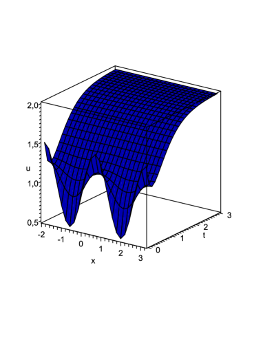
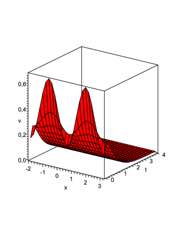
Figure 3: Surfaces representing the $u$ (blue) and $v$ (red) components of solution (75) with $C_{1}=-2,\ C_{2}=5,\ \alpha_{0}=2,\ \alpha_{1}=1$ of system (74) with the parameters $a_{1}=3,\ a_{2}=2,\ b=\frac{3}{2},\ c=3,\ \lambda_{1}=\frac{3}{4},\ \lambda_{2}=1.$

In real-world applications, competition usually occurs in bounded domains. Let us consider the domain $\Omega_{*}=\left\{(t,x)\in(0,+\infty)\times(A,B)\right\},\ -\infty<A<B<+\infty$. Typically, zero flux conditions are prescribed at the boundaries:

$$\begin{array}[]{l}x=A:\,u_{x}=0,\,v_{x}=0,\\ x=B:\,u_{x}=0,\,v_{x}=0.\end{array}$$

The zero flux conditions reflect a natural assumption that the competing species cannot cross the boundaries (e.g., a wide river could be a natural obstacle). One easily checks that the exact solution (75) satisfies the boundary conditions provided

$$A=\frac{\pi}{\kappa}\left(\frac{1}{2}+m_{1}\right),\,B=\frac{\pi}{\kappa}\left(\frac{1}{2}+m_{2}\right),\ m_{1}<m_{2}.$$

Here $m_{1}$ and $m_{2}$ are arbitrary integer parameters and $\kappa=\sqrt{\frac{\lambda_{1}a_{2}-\lambda_{2}a_{1}}{\lambda_{1}-\lambda_{2}}}.$ Thus, we conclude that the exact solution (75) with correctly-specified parameters simulates the competition of two population of species in the bounded domain. An example is presented in Fig. 3.

7 Exact solutions of the three-component DLV system

This section is a natural continuation of the previous one. The only difference is that here a three-component DLV system is studied instead of a two-component system. It should be pointed out that the three-component DLV system (16) admits a much wider set of $Q$-conditional symmetries compared to the two-component analogue. One may apply each $Q$-conditional symmetry arising in Table 5 in order to find exact solutions for the biologically motivated DLV system.

One notes that the DLV systems arising in Cases 1–4 of Table 5 can be reduced to those modeling different types of interaction between three populations of species (cells, chemicals etc.). Here we examine in details only Case 4 because the corresponding symmetry operators have the most complicated structure (Cases 1–3 can be examined in a quite similar way) and present the results derived in [34]. Obviously, the system from Case 4 of is reducible by the substitution $u\to-bu,\ v\to-cv,\ w\to-ew$ to the system

$$\begin{array}[]{l}\lambda_{1}u_{t}=u_{xx}+u(a_{1}-bu-cv-ew),\\ \lambda_{2}v_{t}=v_{xx}+v(a_{2}-bu-cv-ew),\\ \lambda_{3}w_{t}=w_{xx}+w(a_{3}-bu-cv-ew),\end{array}$$ (77)

where the parameters $a_{k},\ b,\ c$ and $e$ are positive constants. System (77) can be used, in particular, for modeling three competing species in the population dynamics.

Let as assume that the coefficients $a_{k}$ and $\lambda_{k}\ (k=1,2,3)$ satisfy the restrictions presented in Case 4 of Table 5. It means that the system admits the symmetry operators $Q^{4}_{i}\ (i=1,\dots,6)$, which have the same structure. Substituting $u\to-bu,\ v\to-cv,\ w\to-ew$ into, e.g., the $Q$-conditional symmetry operator $Q^{4}_{1}$ we obtain

$$Q^{4}_{1}\to Q=\partial_{t}+\frac{a_{1}-a_{2}}{\lambda_{1}-\lambda_{2}}\,u\left(\partial_{u}-\frac{b}{c}\,\partial_{v}\right)+\alpha b\,u\left(\frac{1}{c}\,\partial_{v}-\frac{1}{e}\,\partial_{w}\right).$$ (78)

So, using the standard algorithm to reduce the given PDE system to an ODE system via the known operator (78), one can easily obtain the ansatz

$$\begin{array}[]{l}u=\frac{\varphi_{1}(x)}{b}\,e^{\delta t},\vskip 6.0pt plus 2.0pt minus 2.0pt\\ v=\frac{\varphi_{2}(x)}{c}+\left(\frac{\alpha}{\delta}-1\right)\frac{\varphi_{1}(x)}{c}\,e^{\delta t},\vskip 6.0pt plus 2.0pt minus 2.0pt\\ w=\frac{\varphi_{3}(x)}{e}-\frac{\alpha}{e\delta}\,\varphi_{1}(x)\,e^{\delta t},\ \,\delta=\frac{a_{1}-a_{2}}{\lambda_{1}-\lambda_{2}}\not=0,\end{array}$$ (79)

where $\varphi_{1}(x)$, $\varphi_{2}(x)$ and $\varphi_{3}(x)$ are to-be-determined functions. Substituting ansatz (79) into (77) and taking into account the restriction

$$(\lambda_{2}-\lambda_{3})a_{1}-(\lambda_{1}-\lambda_{3})a_{2}+(\lambda_{1}-\lambda_{2})a_{3}=0$$

(see Case 4 of Table 5), we arrive at the reduced system of ODEs

$$\begin{array}[]{l}\varphi_{1}^{\prime\prime}+\varphi_{1}\left(\frac{\lambda_{1}a_{2}-\lambda_{2}a_{1}}{\lambda_{1}-\lambda_{2}}-\varphi_{2}-\varphi_{3}\right)=0,\\ \varphi_{2}^{\prime\prime}+\varphi_{2}\left(a_{2}-\varphi_{2}-\varphi_{3}\right)=0,\\ \varphi_{3}^{\prime\prime}+\varphi_{3}\left(a_{3}-\varphi_{2}-\varphi_{3}\right)=0.\end{array}$$ (80)

Thus, exact solutions of the three-component competition system (77) can be obtained by substitution of arbitrary solutions of system (80) into ansatz (79).

System (80) is three-component system of nonlinear second-order ODEs. To the best of our knowledge, its general solution is unknown. Let us assume that the triplet $(\varphi^{0}_{1}(x),\varphi^{0}_{2}(x),\varphi^{0}_{3}(x))$ is a particular solution of (80). Moreover, we assume that the functions $\varphi^{0}_{k}$ are nonnegative and bounded on a space interval $I$. Having this, we observe that the exact solution (79) with $\varphi_{k}=\varphi^{0}_{k}\ (k=1,2,3)$ tends to the steady-state solution $\left(0,\frac{\varphi^{0}_{2}}{c},\frac{\varphi^{0}_{3}}{e}\right)$ of the DLV system (77) with $\delta<0$ provided $t\to+\infty$. In the general case, the solution $\left(0,\frac{\varphi^{0}_{2}}{c},\frac{\varphi^{0}_{3}}{e}\right)$ produces a curve in the phase space $(u,v,w)$, which lies in the plane $(0,v,w)$. So, considering the competition of three populations at the space interval $I$, we conclude that the exact solution (79) with $\varphi_{k}=\varphi^{0}_{k}$ $(k=1,2,3)$ describes such competition when species $u$ dies out while species $v$ and $w$ coexist. In particular, a limit cycle may occur if the concentrations $v=\frac{\varphi^{0}_{2}(x)}{c}$ and $w=\frac{\varphi^{0}_{3}(x)}{e}$ form a closed curve.

Let us consider an example in the case when $\varphi^{0}_{2}(x)$ and $\varphi^{0}_{3}(x)$ are constants. It can easily checked that the constant solution $\varphi_{2}=v_{0},\ \varphi_{3}=a_{2}-v_{0}$ of the second and third equations of (80) with $a_{2}=a_{3}$, generates the following solution of the three-component competition system (77) with $a_{1}\neq a_{2}=a_{3}$:

$$\begin{array}[]{l}u=\frac{\varphi_{1}(x)}{b}e^{\delta t},\\ v=\frac{v_{0}}{c}+\frac{1}{c}\left(\frac{\alpha}{\delta}-1\right)\varphi_{1}(x)e^{\delta t},\\ w=\frac{a_{2}-v_{0}}{e}-\frac{\alpha\varphi_{1}(x)}{e\delta}e^{\delta t},\end{array}$$ (81)

where $\varphi_{1}(x)$ is a solution of the linear ODE

$$\varphi_{1}^{\prime\prime}-\lambda_{2}\delta\,\varphi_{1}=0.$$ (82)

Interestingly, the exact solution (81) is not obtainable by any Lie symmetry because system (77) admits the Li algebra (15), so that only traveling wave solutions can be constructed.

We point out that the general solution of ODE (82) essentially depends on the sign of $\delta$. In the case $\delta>0$, unbounded (in time) solutions (see formulae (81)) are obtained and it is unlikely that they can describe a realistic competition between three populations.

On the other hand, equation (82) with $\delta<0$ has the general solution

$$\varphi(x)=C_{1}\cos\left(\sqrt{-\delta\lambda_{2}}\,x\right)+C_{2}\sin\left(\sqrt{-\delta\lambda_{2}}\,x\right),$$ (83)

where $C_{1}$ and $C_{2}$ are arbitrary constants. Setting, for example, $C_{1}=0$ and $C_{2}=1$ in (83) and substituting $\varphi(x)$ into (81), we obtain the exact solution

$$\begin{array}[]{l}u=\frac{1}{b}\sin\left(\sqrt{-\delta\lambda_{2}}\,x\right)e^{\delta t},\\ v=\frac{v_{0}}{c}+\frac{1}{c}\left(\frac{\alpha}{\delta}-1\right)\sin\left(\sqrt{-\delta\lambda_{2}}\,x\right)e^{\delta t},\\ w=\frac{a_{2}-v_{0}}{e}-\frac{\alpha}{e\delta}\sin\left(\sqrt{-\delta\lambda_{2}}\,x\right)e^{\delta t}\end{array}$$ (84)

of system (77) with $a_{1}\neq a_{2}=a_{3},\ \delta=\frac{a_{1}-a_{2}}{\lambda_{1}-\lambda_{2}}.$

Let us provide a biological interpretation of the exact solution (84). For these purposes, we assume that the competition between three populations occurs at the space interval $I=\left[0,\frac{\pi}{\sqrt{-\delta\lambda_{2}}}\right]$. Obviously, the components of the exact solution (84) satisfy the boundary conditions

$$\begin{array}[]{l}x=0:\ u=0,\ v=\frac{v_{0}}{c},\ w=\frac{a_{2}-v_{0}}{e};\\ x=\frac{\pi}{\sqrt{-\delta\lambda_{2}}}:\ u=0,\ v=\frac{v_{0}}{c},\ w=\frac{a_{2}-v_{0}}{e}.\end{array}$$

These conditions predict that the densities of the species $u,\ v$ and $w$ are constant values at the boundaries (it means that an artificial regulation of the population densities holds in a vicinity of the $x=0$ and $x=\frac{\pi}{\sqrt{-\delta\lambda_{2}}}$ points). Moreover, this exact solution tends to the steady-state point $\left(0,\ \frac{v_{0}}{c},\ \frac{a_{2}-v_{0}}{e}\right)$ if $t\rightarrow+\infty.$

It can be checked that all the components in (84) are bounded and nonnegative for an arbitrary given $t>0$ and $x\in I$ provided the additional restrictions

$$\begin{array}[]{l}0\leq v_{0}\leq a_{2}-\frac{\alpha}{\delta},\ \mbox{if}\ \alpha\leq\delta,\\ 1-\frac{\alpha}{\delta}\leq v_{0}\leq a_{2}-\frac{\alpha}{\delta},\ \mbox{if}\ \delta<\alpha\leq 0,\\ 1-\frac{\alpha}{\delta}\leq v_{0}\leq a_{2},\ \mbox{if}\ \alpha>0\end{array}$$

hold. Thus, the exact solution (84) describes the following scenarios of the competition between three species:

• species $v$ and $w$ eventually coexist while species $u$ dies out provided

  $$0<v_{0}<a_{2};$$

• species $v$ eventually dominates while species $u$ and $w$ die out provided

  $$v_{0}=a_{2};$$

• species $w$ eventually dominates while species $u$ and $v$ die out provided

  $$v_{0}=0.$$

Examples of scenarios (i) and (ii) are presented in Fig. 4 and Fig. 5, respectively.

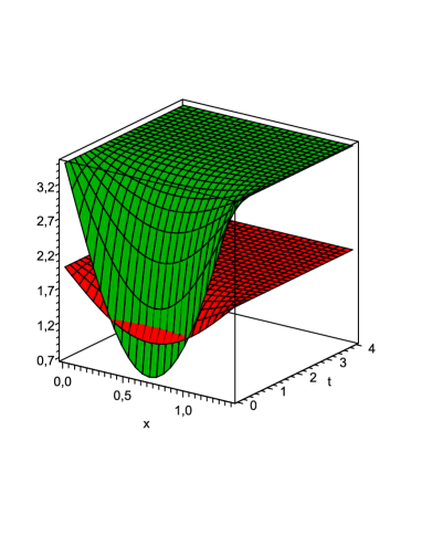
Figure 4: Surfaces representing the $u$ (blue), $v$ (red) and $w$ (green) components of solution (84) with $\alpha=-1,\ v_{0}=\frac{3}{2},\ \delta=-\frac{5}{2}$ of system (77) with the parameters $a_{1}=\frac{9}{2},\ a_{2}=a_{3}=2,\ b=\frac{1}{2},\ c=\frac{3}{4},\ e=\frac{1}{7},\ \lambda_{1}=1,\ \lambda_{2}=\lambda_{3}=2.$

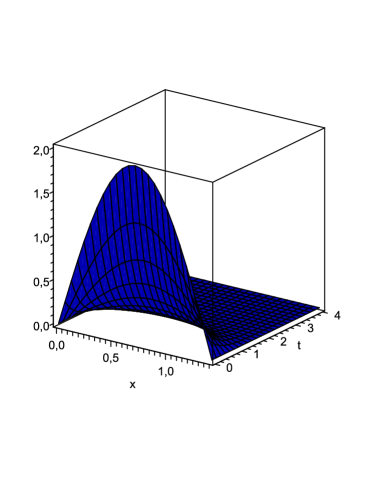
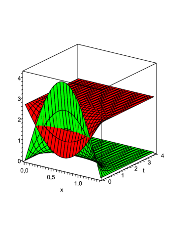
Figure 5: Surfaces representing the $u$ (blue), $v$ (red) and $w$ (green) components of solution (84) with $\alpha=\frac{3}{2},\ v_{0}=2,\ \delta=-\frac{5}{2}$ of system (77) with the parameters $a_{1}=\frac{9}{2},\ a_{2}=a_{3}=2,\ b=\frac{1}{2},\ c=\frac{3}{4},\ e=\frac{1}{7},\ \lambda_{1}=1,\ \lambda_{2}=\lambda_{3}=2.$

An essential progress in constructing exact solutions of the three-component DLV system was achieved in [35]. New exact solutions were discovered when system (16) involves equal diffusivities (i.e. $\lambda_{1}=\lambda_{2}=\lambda_{3}$), positive $a_{i}$ and negative $b_{i},\ c_{i},$ and $e_{i}$ parameters (i.e. describes competition of three populations). In this case, the DLV system (16) is reducible to the form

$$\begin{array}[]{l}u_{t}=u_{xx}+u(1-u-c_{1}v-e_{1}w),\\ v_{t}=v_{xx}+c_{2}v(1-b_{2}u-v-e_{2}w),\\ w_{t}=w_{xx}+e_{3}w(1-b_{3}u-c_{3}v-w)\end{array}$$ (85)

Assuming that linear terms $1-u-c_{1}v-e_{1}w$, $1-b_{2}u-v-e_{2}w$ and $1-b_{3}u-c_{3}v-w$ arising in the RHS of the system are linearly dependent, the following family of exact solutions was derived

$$\begin{array}[]{l}u(t,x)=\frac{c_{1}-1}{c_{1}b_{2}-1}+\frac{e_{1}-c_{1}e_{2}}{c_{1}b_{2}-1}\left(w_{0}+\frac{1}{\sqrt{4\pi t}}\int\limits_{-\infty}^{\ \ \infty}\exp\left(-\frac{(x-y)^{2}}{4t}\right)f(y)dy\right),\vskip 6.0pt plus 2.0pt minus 2.0pt\\ v(t,x)=\frac{b_{2}-1}{c_{1}b_{2}-1}+\frac{e_{2}-b_{2}e_{1}}{c_{1}b_{2}-1}\left(w_{0}+\frac{1}{\sqrt{4\pi t}}\int\limits_{-\infty}^{\ \ \infty}\exp\left(-\frac{(x-y)^{2}}{4t}\right)f(y)dy\right),\vskip 6.0pt plus 2.0pt minus 2.0pt\\ w(t,x)=w_{0}+\frac{1}{\sqrt{4\pi t}}\int\limits_{-\infty}^{\ \ \infty}\exp\left(-\frac{(x-y)^{2}}{4t}\right)f(y)dy,\end{array}$$ (86)

where $w_{0}$ is an arbitrary constant, while $f(y)$ is an arbitrary continuous function such that the integral in the RHS of (86) converges.

Although this result is formulated in the form of a cumbersome theorem (see Theorem 2.1 in [35]), the main idea is very simple and was implicitly used earlier in [23]. In fact, according to the assumption, there exist constants $A,\ B,$ and $C$ such that

$$A(1-u-c_{1}v-e_{1}w)+B(1-b_{2}u-v-e_{2}w)+C(1-b_{3}u-c_{3}v-w)=0.$$

So, taking the linear combination of equations from (86), we exactly arrive at the linear diffusion equation

$$U_{t}=U_{xx},\quad U=Au+Bv+Cw$$ (87)

with correctly-specified $A,\ B$ and $C$. Obviously, the integral in the RHS of (86) is the well-known solution of (87).

In particular case, solution (86) with $f(y)=\beta\sin(\gamma y)$ (here $\beta$ and $\gamma$ are nonzero constants) takes the form [35]

$$\begin{array}[]{l}u(t,x)=\frac{c_{1}-1}{c_{1}b_{2}-1}+\frac{e_{1}-c_{1}e_{2}}{c_{1}b_{2}-1}\left(w_{0}+\beta\sin(\gamma x)e^{-\gamma^{2}t}\right),\vskip 6.0pt plus 2.0pt minus 2.0pt\\ v(t,x)=\frac{b_{2}-1}{c_{1}b_{2}-1}+\frac{e_{2}-b_{2}e_{1}}{c_{1}b_{2}-1}\left(w_{0}+\beta\sin(\gamma x)e^{-\gamma^{2}t}\right),\vskip 6.0pt plus 2.0pt minus 2.0pt\\ w(t,x)=w_{0}+\beta\sin(\gamma x)e^{-\gamma^{2}t}.\end{array}$$ (88)

It can be seen that the exact solution (88) is a generalization of solution (84) on the case when all the diffusivities are equal.

8 Conclusions

This work summarizes all known results (up to this date) about methods of integration of the classical Lotka–Volterra systems with diffusion and presents a wide range of exact solutions, which are the most important from applicability point of view. To the best of our knowledge, it is the first attempt in this direction. Because the DLV systems are used for mathematical modeling of an enormous variety of processes in ecology, biology, medicine, chemistry, etc. (see, e.g., well-known books [6, 7, 8, 9, 10, 11, 12]), we believe that it is an appropriate time for such kind of a review.

We would like to point out that exact solutions always play an important role for any nonlinear model describing real-world processes. At the present time, there is no general theory for integrating nonlinear PDEs (system of PDEs). Thus, construction of particular exact solutions for these equations is a highly nontrivial and important problem. Identifying exact solutions in a closed form that have a physical (chemical, medical, biological etc.) interpretation is of fundamental importance. Even exact solution with questionable applications can be important for proper examination of software packages devoted to numerical solving of systems of PDEs. The obtained exact solutions can also be used as test problems to estimate the accuracy of approximate analytical methods for solving of boundary value problems for PDEs.

In this review, the main attention was paid to symmetry-based methods for exact solving the classical Lotka–Volterra systems with diffusion. We briefly presented the relevant theory (Section 2) and application of the theory to find Lie symmetries of the two- and three-component LV systems (Section 3). Furthermore, we applied the simplest Lie symmetries for constructing plane wave solutions, especially traveling fronts, which are the most popular type of exact solutions in the case of nonlinear evolution equations (Section 4). We also presented the most interesting traveling waves derived by other authors, including those from the pioneering work [19]. It turns out that Lie symmetries have rather a limited efficiency if one looks for exact solutions of the DLV systems, therefore we derived wide families of conditional symmetries of the DLV systems under study (Section 5). Finally, the conditional symmetries obtained were used to construct exact solutions with more complicated structures than the traveling fronts. Moreover, examples of applications of some exact solutions for solving real-world models based on the DLV systems are successfully demonstrated (Sections 6 and 7). We also presented an interesting family of exact solutions derived in [35] by an ad hoc technique, which seems to be not related with symmetry-based methods.

In conclusion, we would like to highlight some unsolved problems. In this review, a majority of exact solutions are related to the DLV systems describing the competition of two (three) populations of species (cells). However, there are other types of interaction between species, cells, chemicals etc. In particular, the nonlinear system (6), in which all the parameters $a_{i}$ and $b_{ij}$ are nonnegative, is a model describing mutualism or cooperation (see, e.g., [6, 58]). Obviously, the solutions presented in this work are useful for interactions of such type as well. On the other hand, these solutions are not applicable for the third most common type of interaction between species (cells, chemicals, etc.) leading to prey-predator models. In the two-component prey-predator model, the parameters satisfy the following typical restrictions $a_{1}a_{2}<0,\ c_{1}b_{2}<0$,  $b_{1}\leq 0$ (see the DLV system (13)). It can be seen that Tables 1, 3 and 4 do not contain such types of systems, therefore the relevant exact solutions cannot be found. Moreover, we have checked that the exact solutions derived in the following studies [19, 23, 24, 25, 27, 28, 32, 34] cannot describe the prey-predator interaction either (at least there are not examples highlighting applicability for the interaction of such type). Thus, the problem of finding exact solutions in a closed form for the DLV system (13) modeling the interaction between preys and predators is still unsolved. Probably, traveling fronts of the form (39) are the first example of such exact solutions.

Another problem of construction of exact solutions for the DLV type systems arise when one examines such systems with time-delay in order to take into account, for example, the age of species in the population. Some examples are presented in the very recent paper [59].

The authors are grateful to Yurko Holovach (Lviv, NAS of Ukraine) who brought our attention to the very old papers by Julius Hirniak [3, 4]. R.Ch. is grateful to late Wilhelm Fushchych who encouraged him to study nonlinear systems of reaction-diffusion PDEs using the Lie symmetry method. Professor Fushchych passed away 25 years ago and the authors would like to dedicate this review to his memory.

References

[1] Lotka A.J.
Undamped oscillations derived from the law of mass action. J
Am Chem Soc 1920;42:1595–99.
[2] Volterra V. Variazioni e fluttuazioni del numero
d‘individui in specie animali conviventi. Mem Acad Lincei
1926;2:31–113.
[3] Hirniak J. About periodical chemical reactions (in Ukrainian). Shevchenko Scientific Society in Lviv, Section Math-Nature-Medicine 1908;12:1–8.
[4] Hirniak J. Zur frage der periodischen reaktionen (in German). Zeitschrift für Physikalische Chemie 1911;75:675–680.
[5] Lotka A. Zur theorie der periodischen reaktion (in German). Zeitschrift für Physikalische Chemie
1910;72:508–11.
[19] Rodrigo M., Mimura M.
Exact solutions of a competition-diffusion system. Hiroshima Math J 2000;30:257–70.
[20] Malfliet W., Hereman W. The tanh method: I. Exact solutions of nonlinear evolution and
wave equations. Phys Scripta 1996;54:563–68.
[21] Malfliet W. The tanh method: a tool for solving certain
classes of nonlinear evolution and wave equations. J Comp Appl
Math 2004;164:529–41.
[22] Rodrigo M., Mimura M. Exact solutions of reaction-diffusion systems and nonlinear wave equations. Japan J Indust Appl Math 2001;18:657-696.
[23] Cherniha R., Dutka V. A diffusive
Lotka–Volterra system: Lie symmetries, exact and numerical solutions.
Ukr Math J 2004;56:1665–75.
[24] Hung L.C. Exact traveling wave solutions for diffusive
Lotka–Volterra systems of two competing species. Japan J Indust
Appl Math 2012;29:237–51.
[25] Kudryashov N.A., Zakharchenko A.S. Analytical properties and exact solutions of the Lotka–Volterra competition system. Appl Math Comput 2015;254:219–28.
[26] Ablowitz M., Zeppetella A. Explicit solutions of Fisher’s
equation for a special wave speed. Bull Math Biol 1979;41:835–40.
[27] Hung, L.C. Traveling wave solutions of competitive-cooperative Lotka–Volterra
systems of three species. Nonlinear Anal RWA 2011;12:3691–700.
[28] Chen C.C., Hung L.C., Mimura M., Ueyama D.
Exact travelling wave solutions of three-species competition-diffusion systems.
Discrete Contin Dyn Syst Ser B 2012;17:2653–69.
[29] Chen C.C., Hung L.C. Nonexistence of traveling wave solutions, exact and semi-exact traveling wave solutions for diffusive Lotka–Volterra systems of three competing species.
Commun Pure Appl Anal 2016;15:1451.
[30] Hou X., Leung A.W. Traveling wave solutions for a competitive reaction-diffusion
system and their asymptotics. Nonlinear Anal RWA 2008;9:2196–213.
[31] Leung A.W., Hou X., Feng W.