Efficient and Consistent Bundle Adjustment on Lidar Point Clouds

Abstract

Bundle Adjustment (BA) refers to the problem of simultaneous determination of sensor poses and scene geometry, which is a fundamental problem in robot vision. This paper presents an efficient and consistent bundle adjustment method for lidar sensors. The method employs edge and plane features to represent the scene geometry, and directly minimizes the natural Euclidean distance from each raw point to the respective geometry feature. A nice property of this formulation is that the geometry features can be analytically solved, drastically reducing the dimension of the numerical optimization. To represent and solve the resultant optimization problem more efficiently, this paper then proposes a novel concept point clusters, which encodes all raw points associated to the same feature by a compact set of parameters, the point cluster coordinates. We derive the closed-form derivatives, up to the second order, of the BA optimization based on the point cluster coordinates and show their theoretical properties such as the null spaces and sparsity. Based on these theoretical results, this paper develops an efficient second-order BA solver. Besides estimating the lidar poses, the solver also exploits the second order information to estimate the pose uncertainty caused by measurement noises, leading to consistent estimates of lidar poses. Moreover, thanks to the use of point cluster, the developed solver fundamentally avoids the enumeration of each raw point (which is very time-consuming due to the large number) in all steps of the optimization: cost evaluation, derivatives evaluation and uncertainty evaluation.

The proposed method is extensively evaluated at different levels: consistency, accuracy, and computation efficiency in both simulated and actual environments. Benchmark evaluation on 19 real-world open sequences covering various datasets (Hilti, NTU-VIRAL and UrbanLoco), environments (campus, urban streets, offices, laboratory, and construction sites), lidar types (Ouster OS0-64, Ouster OS1-16, Velodyne HDL 32E), and motion types (handheld, UAV-based, and ground vehicles-based) shows that our method achieves consistently and significantly higher performance than other state-of-the-art counterparts in terms of localization accuracy, mapping quality, and computation efficiency. In particular, our method achieves a mapping accuracy at a level of the lidar measurement noise (i.e., a few centimeters) while processing all sequences in less than half minute on a standard desktop CPU. Finally, we show how our proposed method effectively improves the accuracy and/or computation efficiency of some important robotic techniques, including lidar-inertial odometry, multi-lidar extrinsic calibration, and high-accuracy global mapping. The implementation of our method is open sourced to benefit the robotics community and beyond.

I Introduction

Light detection and ranging (lidar) has become an essential sensing technology for robots to achieve a high level of autonomy [1, 2]. Enabled by the direct, dense, active and accurate (DDAA) depth measurements, lidar sensors have the ability to build a dense and accurate 3D map of the environment in real-time and at a relatively low computation cost. These unique advantages have made lidar sensors essential to a variety of applications that require real-time, dense, and accurate 3D mapping of the environment, such as autonomous driving [3, 4], unmanned aerial vehicles navigation [5, 6, 7], and real-time mobile mapping [8, 9, 10]. This trend becomes even more evident with recent developments in lidar technologies which have enabled the commercialization and mass production of lightweight and high-performance solid-state lidars at a significantly lower cost [11, 12].

The central task of many lidar-based techniques, such as lidar-based odometry, simultaneous localization and mapping (SLAM), and multi-lidar calibration, is to register multiple point clouds, each measured by the lidar at different poses, into a consistent global point cloud map. However, the predominant point cloud registration methods, such as iterative closest point (ICP) [13] and its variants (e.g, generalized-ICP [14]), normal distribution transformation (NDT) [15, 16], and surfel registration [17], allow registration of two point clouds only. Such a pairwise registration leads to an incremental scan registration process for an odometry system (e.g., [18, 19, 20, 17]), which would rapidly accumulate drift, or a repeated pairwise registration process for 3D mapping [21] or multi-lidar calibration [22], which would bring dramatic computation cost. All these necessitate an efficient concurrent multiple scan registration technique.

Concurrent multiple lidar scan registration requires determining all lidar poses and the scene geometry simultaneously, a process referred to as bundle adjustment (BA) in computer vision. Compared to visual BA, which has been well-established in photogrammetry and played a fundamental role in various vital applications, including visual odometry (VO) [23, 24, 25], visual-inertial odometry (VIO) [26, 27], 3D visual reconstruction [28, 29] and multi-camera calibration [30, 31], lidar BA has a similarly fundamental role but is much less mature due to two major challenges. First, lidar has a long measuring range but low resolution between scanning lines. The measured point cloud are sparsely (sometimes even not repeatedly [12]) distributed in a large 3D space, making it difficult (almost impossible) to scan the same point feature in the space across different scans. This has fundamentally prevented the use of straightforward visual bundle adjustment formulation, which is largely based on point features benefiting from the high-resolution images accurately capturing individual point features. The second challenge lies in the large number of raw points (from tens of thousands to million points) collected by a practical lidar sensors. Processing all these points in the lidar BA is extremely computation intensive.

In this work, we propose an efficient and consistent BA framework specifically designed for lidar point clouds. The framework follows our previous work BALM [32], which formulates the lidar BA problem based on edge and plane features that are abundant in lidar scans. The BA formulation naturally minimizes the straightforward Euclidean distance of each point in a scan to the corresponding edge or plane, while the decision variables include the lidar poses and feature (edge and plane) parameters. Furthermore, it is shown that the geometry parameters (i.e., edge and plane) can be solved analytically, leading to an optimization that depends on the lidar poses only. Since the number of geometry features is often large, elimination of these geometry features from the optimization will drastically reduce the optimization dimension (hence time).

A novel design in our proposed BA framework is the point cluster, which summarizes all points of a lidar scan associated to one feature by a compact set of parameters, point cluster coordinates. Based on the point cluster, we derive the closed-form derivatives (up to second order) of the BA optimization with respect to (w.r.t.) its decision variables (i.e., lidar poses). We prove that the formulated BA optimization and the closed-form derivatives can both be represented fully by the point cluster without enumerating the large number of individual points in a lidar scan. The removal of dependence on individual raw points drastically speeds up the evaluation of the cost function and derivatives, which further enables us to develop an efficient and consistent second-order solver, BALM2.0, which is also released on Github to benefit the community. Our experiment video is available on https://youtu.be/MDrIAyhQ-9E.

We conduct extensive evaluations on the proposed BA method. Simulation study shows that the BA method produces consistent lidar pose estimate. Exhaustive benchmark comparison on 19 real-world open sequences shows that the BA method produces consistently higher performance (pose estimation accuracy, mapping accuracy, and computation efficiency) than other counterparts. We finally integrate the BA method in three vital lidar applications: lidar-inertial odometry, multi-lidar calibration, and global mapping, and show how their accuracy and/or computation efficiency are improved by the proposed BA.

II Related Works

II-A Multi-view registration

The bundle adjustment problem is similar to the multi-view registration problem that has been previously researched [33, 34, 35, 36, 37, 38]. These methods all adopt a two layer framework: the first layer estimates the relative poses of a selected set of scan pairs using the pairwise registration methods (e.g., ICP [13]); From the relative poses, the second layer constructs and solves a pose graph to obtain a maximum a posteriori estimate of all lidar poses. Such a two-layer framework decouples the raw point registration from the global pose estimation, so that each raw point registration only involves a small amount of local points contained in the two scans (instead of all scans sharing overlaps) and the pose graph optimization only involves a small amount of constraints arising from the relative poses (instead of raw points). The net effect is a significant saving of time, hence being largely used in online lidar SLAM systems [39, 40]. However, the advantage in computation efficiency comes with fundamental limitation in accuracy: the pairwise scan registration only considers the overlap among two scan at a time, while the overlap is really shared by all scans and should be registered concurrently. Moreover, the pose graph optimization only considers constraints from the relative poses, while the mapping consistency indicated by the raw points are completely ignored. Consequently, it is usually difficult to produce (or even be aware of) a globally consistent map that is necessary for high-accuracy localization and mapping tasks.

Some early works in computer vision and computer graphics have proposed multi-view registration methods that directly optimize the mapping consistency from multiple range images, aiming for consistent surface modeling of 3D objects. [41] is a direct extension of the ICP method, it minimizes the Euclidean distance between a pre-known control point in one scan to all matched control points in the rest scans. Within this framework, [42] uses a quaternion representation in the optimization, and [43] extends the distance between control points to the distance between surfaces around the respective control points. More recently, Zhu et al. [44] proposes a two step registration method: the first step uses a K-means clustering to cluster points from all scans, and the second step estimates the scan poses by minimizing the Euclidean distance between each point in a cluster to the centroid. Since these methods rely on point features in the scan, they require densely populated point cloud (e.g., by depth camera) for extracting such salient point features. While this is not a problem for small object reconstruction for which these methods are designed, it is not the case for scene reconstruction where the LiDAR measurements are very sparse (sometimes even non-repetitive) as explained above.

II-B Bundle or plane adjustment

In recent years, researchers in the robotics community have shown increasing interests to address the bundle adjustment problem on (lidar) point clouds more formally. Kaess [45] exploits the plane features in the bundle adjustment and minimizes the difference between the plane measured in a scan and the plane predicted from the optimization variables: scan poses and plane parameters. This formulation was later integrated into a key-frame-based online SLAM system [46]. Since the method minimizes the plane-to-plane distance, it requires to segment each scan and estimate the contained local planes in advance. Such plane segmentation and estimation usually require dense point clouds measured by RGB-D cameras on which the work were demonstrated.

A more formal bundle adjustment method on lidar point cloud, termed as the plannar (bundle) adjustment, was later proposed in [47] which minimizes the natural Euclidean distance between each point in a scan to the plane predicted from the scan poses and plane parameters (the optimization variables). Compared with plane-to-plane distance in [45], the point-to-plane metric is faster, more accurate, and more suitable for lidar sensors, where local plane segmentation or estimation are less reliable due to sparse point clouds. Moreover, the direct use of raw points in the point-to-plane metric could also lead to a more consistent estimate of the optimization variables by considering the measurement noises in the raw points. Then, the formulated non-linear least square problem is solved by a Levenberg-Marquardt (LM) algorithm. To lower the computation load caused by the large number of points measurements associated to the same plane feature, [47] propose a reduction technique to eliminate the enumeration of individual points in the evaluation of the residual and Jacobian. Furthermore, due to the very similar structure to the visual bundle adjustment, the proposed bundle adjustment is also compatible with the Schur complement trick [48], which eliminates the plane parameters in each iteration of the LM algorithm. This plane adjustment method is largely used in many online lidar SLAM systems developed subsequently [49, 50] or before [51, 52].

On the other hand, Ferrer [53] exploits plane features similar to [47] and minimizes any deviation of each raw point from the plane equation. The resultant optimization cost then reduces to the minimum eigenvalue of a covariance matrix and is thus termed as the eigen-factor. The author further derived the closed-form gradient of the cost function w.r.t. to both the scan poses and plane parameters and employed a gradient-based method to solve the optimization iteratively. Due to the second order nature of the eigenvalue (as confirmed in [32], see below), the gradient method converges very slowly (requiring a few hundreds of iterations) [53, 50].

Our previous work BALM [32] takes another step towards more efficient bundle adjustment. Similar to [47], BALM minimizes the natural Euclidean distance between each point in a scan to the plane (i.e., point-to-plane metric). Most importantly, BALM proved that the point-to-plane distance is essentially equivalent to the eigen-factor in [53], thus unifying the two metrics in [47] and [53]. It was further proved that all plane parameters can be analytically solved with closed-form solutions in advance, hence the large number of plane parameters can be completely removed from the resultant optimization. Such feature elimination significantly lowered the optimization dimension and poses a fundamental difference from all the previous plannar adjustment methods [51, 53, 47, 49, 50] and visual bundle adjustment methods [48]. The feature elimination also removed the various issues in the plane representation from the optimization, such as normal constraint in the Hesse normal representation $(\mathbf{n},d)$ [53, 47, 49, 50], singularity issue in the closest-point (CP) representation $\mathbf{n}d$ [51] and over-parameterization issue in the quaternion representation [45]. A further advantage of BALM against previous method [51, 53, 47] is that the whole framework is naturally extendable to edge features besides plane features. To solve the resultant optimization problem, BALM [32] subsequently derived the second order derivatives of the cost function and developed a LM-like second-order solver. The developed BA method and solver are very efficient, achieving real-time sliding window optimization when integrated to LOAM [18].

A major drawback of the BALM [32] is that the evaluation of the second-order derivatives including Jacobian and Hessian requires to enumerate each individual lidar point, leading to a computational complexity of $O(N^{2})$ where $N$ is the number of points [50]. Consequently, the method is hard to be used in large-scale problems where the lidar points are huge in number. This problem is partially addressed in [54], which aggregates all points associated to the same plane feature in a scan in the scan local frame. However, to ensure convergence, [54] modifies the cost function by including an extra heuristic penalty term, which is not a true representation of the map consistency. Moreover, the cost function in [54] still involves the plane feature similar to [51, 53, 47, 49, 50]. To lower the computation load caused by optimizing the large number of feature parameters, the method further fixes the feature parameters in the optimisation, which could slow down the optimisation speed.

Our BA formulation in this paper is based on BALM [32], hence inheriting the fundamental feature elimination advantage when compared to [51, 53, 47, 49, 50]. To address the computational complexity of $O(N^{2})$ in BALM, we propose a novel point cluster concept, which fundamentally eliminates the enumeration of each individual point in the evaluation of the cost function, Jacobian and Hessian matrix. Consequently, the computational complexity is irrelevant to both the feature dimension (similar to BALM [32]) and the point number (similar to [47, 49]). The point cluster in our method is similar to the point aggregation used in [54], but the overall BA formulation is fundamentally different: (1) it minimizes the true map consistency (the point-to-plane distance) without trading off with any other heuristic penalty; and (2) it performs exact feature elimination with rigorous proof instead of empirical fixation. Based on these nice theoretical results, we develop an efficient second-order solver, termed as BALM2.0. Besides solving the nominal lidar poses, the solver also estimates the uncertainty of the estimated lidar pose by leveraging the second-order derivative information, which is another new contribution compared with existing works.

III Bundle Adjustment Formulation and Optimization

TABLE I: Nomenclatures

Notation	Explanation
$\mathbb{R}^{m\times n}$	The set of $m\times n$ real matrices.
$\mathbb{S}^{m\times m}$	The set of $m\times m$ symmetric matrices.
$\boxplus$	The encapsulated “boxplus” operations on manifold.
$(\cdot)_{f}$	The value of $(\cdot)$ expressed in lidar local frame,
$(\cdot)$	The value of $(\cdot)$ expressed in global frame.
$\lfloor\cdot\rfloor$	The skew symmetric matrix of $(\cdot)$.
$\exp(\cdot)$	Exponential of $(\cdot)$, which could be a matrix.
$\mathbbm{1}_{i=j}$	Indicator function which is equal to “$1$” if $i=j$,
	otherwise equal to “$0$”.
$M_{f},M_{p}$	The number of features and poses, respectively.
$i,j,k$	The indexes of features, poses and points, respectively.
$l$	The index of eigenvalue and eigenvector of a matrix.
p,q	The indexes of (block) row and column in a matrix.
$\mathbf{e}_{l}$	The vector in $\mathbb{R}^{4}$ with all elements being zeros except
	the $l$-th element being one ($l\in\{1,2,3,4\}$).
$\mathbf{S}_{\text{\bf P}}$	$\mathbf{S}_{\text{\bf P}}=\begin{bmatrix}\mathbf{I}_{3\times 3}&\mathbf{0}_{3\times 1}\end{bmatrix}\in\mathbb{R}^{3\times 4}$.
$\mathbf{S}_{\text{\bf v}}$	$\mathbf{S}_{\text{\bf P}}=\begin{bmatrix}\mathbf{0}_{1\times 3}&1\end{bmatrix}\in\mathbb{R}^{1\times 4}$.
$\mathbf{E}_{kl}$	$\mathbf{E}_{kl}=\mathbf{e}_{k}\mathbf{e}_{l}^{T}+\mathbf{e}_{l}\mathbf{e}_{k}^{T}\in\mathbb{S}^{4\times 4},\ k,l\in\{1,2,3,4\}$.

In this chapter, we derive our BA formulation and optimisation. First, following [32], we formulate the BA as minimizing the the point-to-plane (or point-to-edge) distance (Sec. III-A) and show that the feature parameters can be eliminated from the formulated optimisation (Sec. III-B). Then, we introduce the point cluster in Sec. III-C, based on which the first and second order derivatives are derived in Sec. III-D. Based on these theoretical results, we present our second-order solver in Sec. III-E. Then the time complexity of the proposed BA is analyzed in the Sec. III-F . Finally, in Sec. III-G, we show how to estimate the uncertainty of the BA solution. Throughout this paper, we use notations summarized in Table I or otherwise specified in the context.

III-A BA formulation

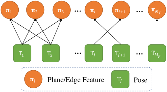
Figure 1: Factor graph representation of the bundle adjustment formulation.

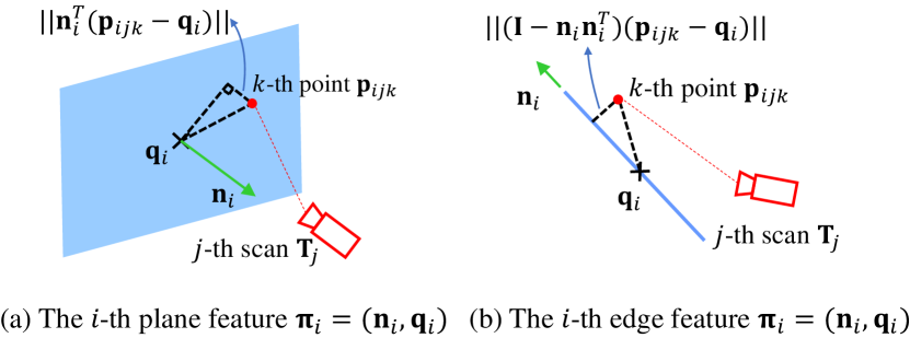
Figure 2: Plane and edge features used in the lidar BA. (a) The plane formulation. $\mathbf{q}_{i}$ is a point in the plane and $\mathbf{n}_{i}$ is the plane normal. (b) The line formulation. $\mathbf{q}_{i}$ is a point on the edge and $\mathbf{n}_{i}$ is the edge direction.

Shown in Fig. 1, assume there are $M_{f}$ features, each denoted by parameter $\boldsymbol{\pi}_{i}$ ($i=1,...,M_{f}$), observed by $M_{p}$ lidar poses, each denoted by $\mathbf{T}_{j}=(\mathbf{R}_{j},\mathbf{t}_{j})$ ($j=1,...,M_{p}$), the bundle adjustment refers to simultaneously determining all the lidar poses (denoted by $\mathbf{T}=(\mathbf{T}_{1},\cdots,\mathbf{T}_{M_{p}})$) and feature parameters (denoted by $\boldsymbol{\pi}=(\boldsymbol{\pi}_{1},\cdots,\boldsymbol{\pi}_{M_{f}})$), such that reconstructed map agrees with the lidar measurements to the best extent. Denote $c(\boldsymbol{\pi}_{i},\mathbf{T})$ the map consistency due to the $i$-th feature, a straightforward BA formulation is

$$\min_{\mathbf{T},\boldsymbol{\pi}}\Big{(}\sum_{i=1}^{M_{f}}c(\boldsymbol{\pi}_{i},\mathbf{T})\Big{)}.$$ (1)

In our BA formulation, we make use of plane and edge features that are often abundant in lidar point cloud and minimize the natural Euclidean distance between each measured raw lidar point and its corresponding plane or edge feature. Specifically, assume a total number of $N_{ij}$ lidar points are measured on the $i$-th feature at the $j$-th lidar pose, each denoted by $\mathbf{p}_{f_{ijk}}$ ($k=1,...,N_{ij}$). Its predicted location in the global frame is

$$\mathbf{p}_{ijk}=\mathbf{R}_{j}\mathbf{p}_{f_{ijk}}+\mathbf{t}_{j}.$$ (2)

For a plane feature, it is parameterized by $\boldsymbol{\pi}_{i}=(\mathbf{n}_{i},\mathbf{q}_{i})$ with $\mathbf{n}_{i}$ the plane normal vector and $\mathbf{q}_{i}$ an arbitrary point on the plane, both in the global frame (see Fig. 2 (a)). Then, the Euclidean distance between a measured point $\mathbf{p}_{f_{ijk}}$ to the plane is $\|\mathbf{n}_{i}^{T}(\mathbf{p}_{ijk}-\mathbf{q}_{i})\|_{2}$. Aggregating the distance for all points observed in all poses leads to the total map consistency corresponding to this plane feature:

$$c(\boldsymbol{\pi}_{i},\mathbf{T})=\frac{1}{N_{i}}\sum_{j=1}^{M_{p}}\sum_{k=1}^{N_{ij}}\left\|\mathbf{n}_{i}^{T}(\mathbf{p}_{ijk}-\mathbf{q}_{i})\right\|_{2}^{2}$$ (3)

where $N_{i}=\sum_{j=1}^{M_{p}}N_{ij}$ is the total number of lidar points observed on the plane feature by all poses.

For an edge feature, it is parameterized by $\boldsymbol{\pi}_{i}=(\mathbf{n}_{i},\mathbf{q}_{i})$ with $\mathbf{n}_{i}$ the edge direction vector and $\mathbf{q}_{i}$ an arbitrary point on the edge, both in the global frame (see Fig. 2 (b)). Then, the Euclidean distance between a measured point $\mathbf{p}_{f_{ijk}}$ to the edge is $\left\|(\mathbf{I}-\mathbf{n}_{i}\mathbf{n}_{i}^{T})(\mathbf{p}_{ijk}-\mathbf{q}_{i})\right\|_{2}$. Aggregating the distance for all points observed in all poses leads to the total map consistency corresponding to this edge feature:

$$c(\boldsymbol{\pi}_{i},\mathbf{T})=\frac{1}{N_{i}}\sum_{j=1}^{M_{p}}\sum_{k=1}^{N_{ij}}\left\|(\mathbf{I}-\mathbf{n}_{i}\mathbf{n}_{i}^{T})(\mathbf{p}_{ijk}-\mathbf{q}_{i})\right\|_{2}^{2}$$ (4)

where $N_{i}=\sum_{j=1}^{M_{p}}N_{ij}$ is the total number of lidar points observed on the edge feature by all poses.

III-B Elimination of feature parameters

In this section, we show that in the BA optimization (1), the feature parameter $\boldsymbol{\pi}$ can really be solved with a closed-form solution. The key observation is that one cost item $c(\boldsymbol{\pi}_{i},\mathbf{T})$ depends solely on one feature parameter, so that the feature parameter can be optimized independently. Concretely,

$$\min_{\mathbf{T},\boldsymbol{\pi}}\Big{(}\sum_{i=1}^{M_{f}}c(\boldsymbol{\pi}_{i},\mathbf{T})\Big{)} =\min_{\mathbf{T}}\Big{(}\min_{\boldsymbol{\pi}}\Big{(}\sum_{i=1}^{M_{f}}c(\boldsymbol{\pi}_{i},\mathbf{T})\Big{)}\Big{)}$$

$$=\min_{\mathbf{T}}\Big{(}\sum_{i=1}^{M_{f}}\min_{\boldsymbol{\pi}_{i}}c(\boldsymbol{\pi}_{i},\mathbf{T})\Big{)}.$$ (5)

In case of a plane feature, we substitute (3) into $c(\boldsymbol{\pi}_{i},\mathbf{T})$:

$$\min_{\boldsymbol{\pi}_{i}}c(\boldsymbol{\pi}_{i},\mathbf{T}) =\min_{\boldsymbol{\pi}_{i}}\Big{(}\frac{1}{N_{i}}\sum_{j=1}^{M_{p}}\sum_{k=1}^{N_{ij}}\left\|\mathbf{n}_{i}^{T}(\mathbf{p}_{ijk}-\mathbf{q}_{i})\right\|_{2}^{2}\Big{)}$$

$$=\lambda_{3}(\mathbf{A}_{i}),\text{ when }\mathbf{n}_{i}^{\star}=\mathbf{u}_{3}(\mathbf{A}_{i}),\mathbf{q}_{i}^{\star}=\bar{\mathbf{p}}_{i}$$ (6)

where $\lambda_{l}(\mathbf{A}_{i})$ denotes the $l$-th largest eigenvalue of matrix $\mathbf{A}_{i}$, $\mathbf{u}_{l}(\mathbf{A}_{i})$ denotes the corresponding eigenvector, the matrix $\mathbf{A}_{i}$ and vector $\bar{\mathbf{p}}_{i}$ are defined as:

$$\mathbf{A}_{i} \triangleq\frac{1}{N_{i}}\sum_{j=1}^{M_{p}}\sum_{k=1}^{N_{ij}}(\mathbf{p}_{ijk}-\bar{\mathbf{p}}_{i}),\ \bar{\mathbf{p}}_{i}\triangleq\frac{1}{N_{i}}\sum_{j=1}^{M_{p}}\sum_{k=1}^{N_{ij}}\mathbf{p}_{ijk}.$$ (7)

The proof will be given in Supplementary II-A [55]. Note that the optimal solution $\mathbf{q}_{i}^{\star}$ in (6) is not unique, any deviation from $\mathbf{q}_{i}^{\star}$ along a direction perpendicular to $\mathbf{n}_{i}^{\star}$ will equally serve the optimal solution. However, these equivalent optimal solution will not change the plane nor the optimal cost (hence the results that follow next). Indeed, the point $\mathbf{q}_{i}^{\star}$ could be an arbitrary point on the plane as it is defined to be.

In case of an edge feature, we substitute (4) into $c(\boldsymbol{\pi}_{i},\mathbf{T})$:

$$\min_{\boldsymbol{\pi}_{i}}c(\boldsymbol{\pi}_{i},\mathbf{T})\!\!=\!\min_{\boldsymbol{\pi}_{i}}\!\Big{(}\frac{1}{N_{i}}\sum_{j=1}^{M_{p}}\sum_{k=1}^{N_{ij}}\left\|(\mathbf{I}-\mathbf{n}_{i}\mathbf{n}_{i}^{T})(\mathbf{p}_{ijk}-\mathbf{q}_{i})\right\|_{2}^{2}\Big{)}$$

$$=\lambda_{2}(\mathbf{A}_{i})+\lambda_{3}(\mathbf{A}_{i});\text{ when }\mathbf{n}_{i}^{\star}=\mathbf{u}_{1}(\mathbf{A}_{i}),\mathbf{q}_{i}^{\star}=\bar{\mathbf{p}}_{i}.$$ (8)

Again, the optimal solution $\mathbf{q}_{i}^{\star}$ in (8) is not unique, any deviation from $\mathbf{q}_{i}^{\star}$ along the direction $\mathbf{n}_{i}^{\star}$ will equally serve the optimal solution. However, these equivalent optimal solution will not change the edge nor the optimal cost (hence the results that follow next).

As can be seen from (6) and (8), the parameter $\boldsymbol{\pi}_{i}$ for each feature, either it is a plane or edge, can be analytically solved and hence removed from the BA optimization process. Consequently, the original BA optimization in (1) reduces to

$$\min_{\mathbf{T}}\Big{(}\sum_{i=1}^{M_{f}}\lambda_{l}(\mathbf{A}_{i})\Big{)}$$ (9)

where $l\in\{2,3\}$ and we omitted the exact number of eigenvalues in the cost function for brevity.

Note that the matrix $\mathbf{A}_{i}$ in (9) depends on the lidar pose $\mathbf{T}$ since each involved point $\mathbf{p}_{ijk}$ depends on the pose (see (7) and (2)). Hence the decision variables of the resultant optimization in (9) involve the lidar pose $\mathbf{T}$ only, which dramatically reduces the optimization dimension (hence computation time).

III-C Point cluster

With the feature parameters eliminated, another difficulty remaining in the BA optimization (9) is that the evaluation of matrix $\mathbf{A}_{i}$ (and its Jacobian or Hessian necessary for developing a numerical solver) requires to enumerate every point observed at each lidar pose. Such an enumeration is extremely computationally expensive due to the large number of points in a lidar scan. In this section, we show such point enumeration can be avoided by a novel concept point cluster, which is detailed as follows.

A point cluster is a finite point set denoted by set $\boldsymbol{\mathcal{C}}=\{\mathbf{p}_{{k}}\in\mathbb{R}^{3}|k=1,\cdots,n\}$, the corresponding point cluster coordinate, denoted as $\boldsymbol{\Re}\!\left(\boldsymbol{\mathcal{C}}\right)$, is defined as:

$$\boldsymbol{\Re}\!\left(\boldsymbol{\mathcal{C}}\right)\triangleq\sum_{k=1}^{n}\begin{bmatrix}\mathbf{p}_{k}\\ 1\end{bmatrix}\begin{bmatrix}\mathbf{p}_{k}^{T}&1\end{bmatrix} =\begin{bmatrix}\mathbf{P}&\mathbf{v}\\ \mathbf{v}^{T}&n\end{bmatrix}\in\mathbb{S}^{4\times 4}$$

$$\mathbf{P}=\sum_{k=1}^{n}\mathbf{p}_{k}\mathbf{p}_{k}^{T},\quad \mathbf{v}=\sum_{k=1}^{n}\mathbf{p}_{k},$$ (10)

where $\mathbb{S}^{4\times 4}$ denotes the set of $4\times 4$ symmetric matrix.

A point cluster can be thought as a generalized point, for which a rigid transform could be applied. Similarly, we can define rigid transformation on a point cluster as follows.

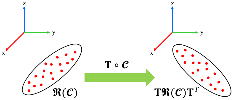
(a) Rigid transform

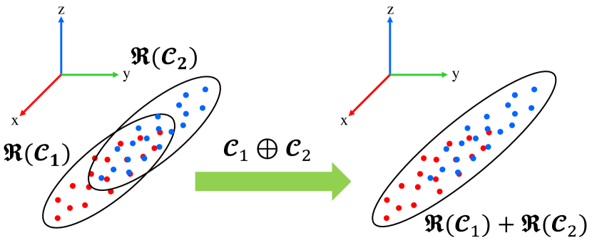
(b) Cluster merging

Figure 3: Two operations on point cluster (a) Rigid transform (b) Cluster merging.

Definition 1.

(Rigid transform) Given a point cluster with point collection $\boldsymbol{\mathcal{C}}=\{\mathbf{p}_{{k}}\in\mathbb{R}^{3}|k=1,\cdots,n\}$ and a pose $\mathbf{T}=\begin{bmatrix}\mathbf{R}&\mathbf{t}\\ 0&1\end{bmatrix}\in SE(3)$. The rigid transformation of the point cluster $\boldsymbol{\mathcal{C}}$, denoted by $\mathbf{T}\circ\boldsymbol{\mathcal{C}}$, is defined as

$$\mathbf{T}\circ\boldsymbol{\mathcal{C}}\triangleq\{\mathbf{R}\mathbf{p}_{{k}}+\mathbf{t}\in\mathbb{R}^{3}|k=1,\cdots,n\}.$$ (11)

Besides rigid transformation, we also define cluster merging operation, as follows.

Definition 2.

(Cluster merging) Given two point clusters with point collections $\boldsymbol{\mathcal{C}}_{1}=\{\mathbf{p}_{k}^{1}\in\mathbb{R}^{3}|k=1,\cdots,n_{1}\}$ and $\boldsymbol{\mathcal{C}}_{2}=\{\mathbf{p}_{{k}}^{2}\in\mathbb{R}^{3}|k=1,\cdots,n_{2}\}$, respectively. The merged cluster, denoted by $\boldsymbol{\mathcal{C}}_{1}\oplus\boldsymbol{\mathcal{C}}_{2}$, is defined as

$$\boldsymbol{\mathcal{C}}_{1}\oplus\boldsymbol{\mathcal{C}}_{2}\triangleq\{\mathbf{p}_{{k}}^{l}\in\mathbb{R}^{3}|l=1,2;k=1,\cdots,n_{i}\}.$$ (12)

Next we will show that the two operations defined above can be fully represented by their point cluster coordinates.

Theorem 1.

Given a point cluster $\boldsymbol{\mathcal{C}}$ and a pose $\mathbf{T}=\begin{bmatrix}\mathbf{R}&\mathbf{t}\\ 0&1\end{bmatrix}\in SE(3)$. The rigid transformation of the point cluster satisfies

$$\boldsymbol{\Re}(\mathbf{T}\circ\boldsymbol{\mathcal{C}})=\mathbf{T}\boldsymbol{\Re}(\boldsymbol{\mathcal{C}})\mathbf{T}^{T}$$ (13)

Proof.

See Supplementary II-B [55]. ∎

Theorem 2.

Given two point clusters $\boldsymbol{\mathcal{C}}_{1}$ and $\boldsymbol{\mathcal{C}}_{2}$. The merged cluster satisfies

$$\boldsymbol{\Re}(\boldsymbol{\mathcal{C}}_{1}\oplus\boldsymbol{\mathcal{C}}_{2})=\boldsymbol{\Re}(\boldsymbol{\mathcal{C}}_{1})+\boldsymbol{\Re}(\boldsymbol{\mathcal{C}}_{2})$$ (14)

Proof.

See Supplementary II-C [55]. ∎

As can be seen, rigid transformation and cluster merging operations on point clusters can be represented by usual matrix multiplication and addition on the point cluster coordinates. A visual illustration of the two operations and their coordinate representations are shown in Fig. 3. These results are crucially important: Theorem 1 indicates that the point cluster can be constructed in one frame (e.g., local lidar frame) and transformed to another (e.g., the global frame) without enumerating each individual points; Theorem 2 indicates that two (and by induction more) point clusters can be further merged to form a new point cluster. A particular case of Theorem 2 is when the second point cluster contains a single point, indicating that the point cluster can be constructed incrementally as lidar points arrives sequentially.

Remark: A point set and its coordinate is not a one-to-one mapping. While it is obvious that the coordinate is uniquely determined from the point set as shown in (10), the reverse way does not hold: the point set cannot be recovered from its coordinate uniquely. Since different point sets may lead to the same coordinate, the raw points must be saved if a re-clustering is needed.

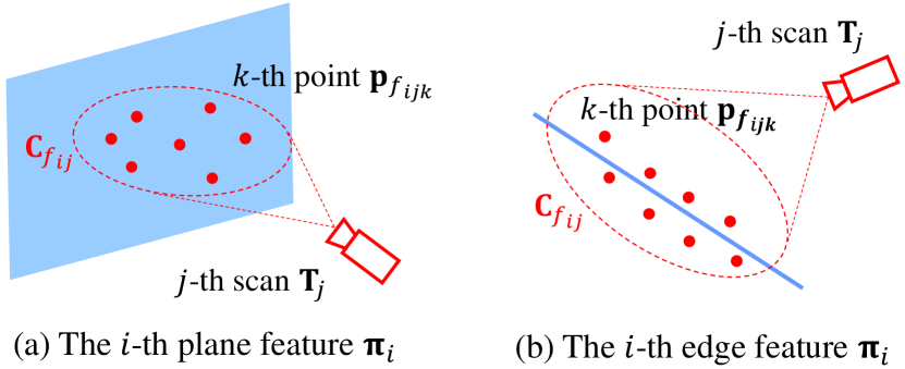
Figure 4: For the $i$-the feature (either plane or edge), all points observed at the $j$-th pose are clustered as a point cluster and is represented by ${\mathbf{C}}_{f_{ij}}$ in its local frame.

Now, we apply the point cluster to the BA problem concerned in this paper. To start with, we group all points on the same feature as a point cluster. For example, the point cluster for the $i$-th feature is $\boldsymbol{\mathcal{C}}_{i}\triangleq\{\mathbf{p}_{ijk}|j=1,\cdots,M_{p},k=1,\cdots,N_{ij}\}$. Denote $\mathbf{C}_{i}$ the coordinate of the point cluster, following (10), we obtain

$$\mathbf{C}_{i} =\boldsymbol{\Re}(\boldsymbol{\mathcal{C}}_{i})\triangleq\sum_{j=1}^{M_{p}}\sum_{k=1}^{N_{ij}}\begin{bmatrix}\mathbf{p}_{ijk}\\ 1\end{bmatrix}\begin{bmatrix}\mathbf{p}_{ijk}^{T}&1\end{bmatrix}=\begin{bmatrix}\mathbf{P}_{i}&\mathbf{v}_{i}\\ \mathbf{v}_{i}^{T}&N_{i}\end{bmatrix}$$

$$\quad\mathbf{P}_{i}=\sum_{j=1}^{M_{p}}\sum_{k=1}^{N_{ij}}\mathbf{p}_{ijk}\mathbf{p}_{ijk}^{T},\quad\mathbf{v}_{i}=\sum_{j=1}^{M_{p}}\sum_{k=1}^{N_{ij}}\mathbf{p}_{ijk}$$ (15)

A key result we show now is that this point cluster coordinate $\mathbf{C}_{i}$ is completely sufficient to represent the matrix $\mathbf{A}_{i}$ required in the BA optimization (9). According to (7), we have

$$\mathbf{A}_{i}= \frac{1}{N_{i}}\sum_{j=1}^{M_{p}}\sum_{k=1}^{N_{ij}}(\mathbf{p}_{ijk}-\bar{\mathbf{p}}_{i})(\mathbf{p}_{ijk}-\bar{\mathbf{p}}_{i})^{T}$$

$$= \frac{1}{N_{i}}\sum_{j=1}^{M_{p}}\sum_{k=1}^{N_{ij}}(\mathbf{p}_{ijk}\mathbf{p}_{ijk}^{T})-\bar{\mathbf{p}}_{i}\bar{\mathbf{p}}_{i}^{T}$$

$$= \frac{1}{N_{i}}\mathbf{P}_{i}-\frac{1}{N_{i}^{2}}\mathbf{v}_{i}\mathbf{v}_{i}^{T}\triangleq\mathbf{A}(\mathbf{C}_{i})$$ (16)

where we denote $\mathbf{A}_{i}$ as a function of $\mathbf{C}_{i}$ since the $\mathbf{A}_{i}$ is fully represented (and uniquely determined) by $\mathbf{C}_{i}$. We slightly abuse the notation here by denoting the function as $\mathbf{A}(\cdot)$.

On the other hand, since the point set $\boldsymbol{\mathcal{C}}_{i}$ is defined on points in the global frame, the coordinate $\mathbf{C}_{i}$ is dependent on the lidar pose, which remains to be optimized. To explicitly parameterize the lidar pose, we note that

$$\boldsymbol{\mathcal{C}}_{i} \triangleq\{\mathbf{p}_{ijk}|j=1,\cdots,M_{p},k=1,\cdots,N_{ij}\}$$ (17)

$$=\cup_{j=1}^{M_{p}}\{\mathbf{p}_{ijk}|k=1,\cdots,N_{ij}\}$$ (18)

$$\stackrel{{\scriptstyle\text{Def.}\ref{def_merge}}}{{=}}\oplus_{j=1}^{M_{p}}\boldsymbol{\mathcal{C}}_{ij},\quad\boldsymbol{\mathcal{C}}_{ij}\triangleq\{\mathbf{p}_{ijk}|k=1,\cdots,N_{ij}\}$$ (19)

$$\stackrel{{\scriptstyle\text{Def.}\ref{def_transform}}}{{=}}\oplus_{j=1}^{M_{p}}\left(\mathbf{T}_{j}\circ\boldsymbol{\mathcal{C}}_{f_{ij}}\right),\ \boldsymbol{\mathcal{C}}_{f_{ij}}\triangleq\{\mathbf{p}_{f_{ijk}}|k=1,\cdots,N_{ij}\}$$ (20)

where $\mathbf{p}_{f_{ijk}}$ is a point represented in the lidar local frame (see (2)), $\boldsymbol{\mathcal{C}}_{{ij}}$ is the point set that is composed of all points on the $i$-th feature (either plane or edge) observed at the $j$-th lidar pose, and $\boldsymbol{\mathcal{C}}_{f_{ij}}$ is the same point set as $\boldsymbol{\mathcal{C}}_{{ij}}$, but represented in the lidar local frame (see Fig. 4).

The relation between the point cluster $\boldsymbol{\mathcal{C}}_{i}$ and $\boldsymbol{\mathcal{C}}_{f_{ij}}$ shown in (20) will lead to a relation between their coordinates $\mathbf{C}_{i}$ and $\mathbf{C}_{f_{ij}}$ as below:

$$\mathbf{C}_{i}\stackrel{{\scriptstyle\text{Thm.}\ref{theorem_merge}}}{{=}}\sum_{j=1}^{M_{p}}\mathbf{C}_{ij}\stackrel{{\scriptstyle\text{Thm.}\ref{theorem_transform}}}{{=}}\sum_{j=1}^{M_{p}}\mathbf{T}_{j}\mathbf{C}_{f_{ij}}\mathbf{T}_{j}^{T}$$ (21)

As a result, the BA optimization in (9) further reduces to

$$\min_{\mathbf{T}_{j}\in SE(3),\forall j}\underbrace{\left(\sum_{i=1}^{M_{f}}\lambda_{l}\left(\mathbf{A}\left(\sum_{j=1}^{M_{p}}\mathbf{T}_{j}\mathbf{C}_{f_{ij}}\mathbf{T}_{j}^{T}\right)\right)\right)}_{c(\mathbf{T})}$$ (22)

where the function $\mathbf{A}(\cdot)$ is defined in (16). Note that the cost function in (22) only requires the knowledge of point cluster coordinate $\mathbf{C}_{f_{ij}}$ without enumerating each individual points. The coordinate $\mathbf{C}_{f_{ij}}$ is computed as (following (10)):

$$\mathbf{C}_{f_{ij}} =\begin{bmatrix}\mathbf{P}_{f_{ij}}&\mathbf{v}_{f_{ij}}\\ \mathbf{v}_{f_{ij}}^{T}&N_{ij}\end{bmatrix}$$

$$\mathbf{P}_{f_{ij}} =\sum_{k=1}^{N_{ij}}\mathbf{p}_{f_{ijk}}\mathbf{p}_{f_{ijk}}^{T},\quad\mathbf{v}_{f_{ij}}=\sum_{k=1}^{N_{ij}}\mathbf{p}_{f_{ijk}}$$ (23)

which can be constructed during the feature association stage before the optimization. In particular, if the $j$-th pose observes no point on the $i$-th feature, $\mathbf{C}_{f_{ij}}=\mathbf{0}_{4\times 4}$, which will naturally remove the dependence on the $j$-th pose for the $i$-th cost item as shown in (22).

Theorem 3.

Given a matrix function $\mathbf{A}(\mathbf{C})\triangleq\frac{1}{N}\mathbf{P}-\frac{1}{N^{2}}\mathbf{v}\mathbf{v}^{T}$ with $\mathbf{C}=\begin{bmatrix}\mathbf{P}&\mathbf{v}\\ \mathbf{v}^{T}&N\end{bmatrix}\in\mathbb{S}^{4\times 4}$, $\lambda_{l}(\mathbf{A})$ denotes the $l$-th largest eigenvalue of $\mathbf{A}$, then $\lambda_{l}(\mathbf{A}(\mathbf{C}))$ is invariant to any rigid transformation $\mathbf{T}_{0}\in SE(3)$. That is,

$$\lambda_{l}\left(\mathbf{A}\left(\mathbf{T}_{0}\mathbf{C}\mathbf{T}_{0}^{T}\right)\right)=\lambda_{l}\left(\mathbf{A}\left(\mathbf{C}\right)\right),\forall\mathbf{T}_{0}\in SE(3).$$ (24)

Proof.

See Supplementary II-D [55]. ∎

Theorem 3 implies that left multiplying all poses $\mathbf{T}_{j},\forall j,$ by the same transform $\mathbf{T}_{0}$ does not change the optimization at all. That is, the BA optimization is invariant to the change of the global reference frame, which is the well-known gauge freedom in a bundle adjustment problem.

III-D First and Second Order Derivatives

As shown in the previous section, the BA optimization problem in (22) is completely equivalent to the original formulation (1), where each cost item standards for the squared Euclidean distance from a point to a plane (or edge). This squared distance is essentially a quadratic optimization, which requires the knowledge of the second-order information of the cost function for efficient solving. In this section, we derive such first and second order derivatives. Without loss of generality, we only discuss the $i$-th feature, which contributes a cost item in the form of

$$c_{i}(\mathbf{T})=\lambda_{l}\left(\mathbf{A}\left(\sum_{j=1}^{M_{p}}\mathbf{T}_{j}\mathbf{C}_{f_{ij}}\mathbf{T}_{j}^{T}\right)\right)$$ (25)

with $\mathbf{C}_{f_{ij}}\in\mathbb{R}^{4\times 4}$ being a pre-computed matrix (see (23)).

To derive the derivative of the cost item (25) w.r.t. the pose $\mathbf{T}_{j}$, which is an element of the Special Euclidean group $SE(3)$, we parameterize its perturbation by a special addition, called boxplus ($\boxplus$-operation). For the pose vector $\mathbf{T}=(\cdots,\mathbf{T}_{j},\cdots)$, we define the the $\boxplus$ operation as below

$$\mathbf{T}\boxplus\delta\mathbf{T} \triangleq(\cdots,\mathbf{T}_{j}\boxplus\delta\mathbf{T}_{j},\cdots),$$ (26)

$$\mathbf{T}_{j}\boxplus\delta\mathbf{T}_{j} \triangleq(\exp{(\lfloor\delta\boldsymbol{\phi}_{j}\rfloor)}\mathbf{R}_{j},\delta\mathbf{t}_{j}+\exp{(\lfloor\delta\boldsymbol{\phi}_{j}\rfloor)}\mathbf{t}_{j}),$$ (27)

where $\delta\mathbf{T}\triangleq(\cdots,\delta\mathbf{T}_{j},\cdots)\in\mathbb{R}^{6M_{p}}$ with $\delta\mathbf{T}_{j}\triangleq(\delta\boldsymbol{\phi}_{j},\delta\mathbf{t}_{j})\in\mathbb{R}^{6},\forall j,$ is the perturbation on the pose vector.

For a scalar function $f(\mathbf{T}):SE(3)\times\cdots\times SE(3)\mapsto\mathbb{R}$, denote $\left(\frac{\partial{f(\mathbf{T})}}{\partial\mathbf{T}}\right)(\mathbf{T}_{0})$ its first-order derivative and $\left(\frac{\partial{f^{2}(\mathbf{T})}}{\partial\mathbf{T}^{2}}\right)(\mathbf{T}_{0})$ its second-order derivative, both at a chosen point of the input $\mathbf{T}_{0}$. The $\boxplus$ operation enables us to parameterize the input of function $f(\cdot)$, $\mathbf{T}$, by its perturbation $\delta\mathbf{T}$ from a given point $\mathbf{T}_{0}$: $\mathbf{T}=\mathbf{T}_{0}\boxplus\delta\mathbf{T}$. Since the map between $\mathbf{T}$ and $\delta\mathbf{T}$ is bijective if $\|\delta\boldsymbol{\phi}_{j}\|<\pi,\forall j$, the scalar function $f(\mathbf{T})$ in terms of $\mathbf{T}$ can be equivalently written as a function $f(\mathbf{T}_{0}\boxplus\delta\mathbf{T})$ in terms of $\delta\mathbf{T}$. As a consequence, the derivatives of $f(\mathbf{T})$ w.r.t. $\mathbf{T}$ at the point $\mathbf{T}_{0}$ can be defined as the derivatives of $f(\mathbf{T}_{0}\boxplus\delta\mathbf{T})$ w.r.t. $\delta\mathbf{T}$ at zero, where the latter is a normal derivative w.r.t. Euclidean vectors:

$$\left(\frac{\partial f(\mathbf{T})}{\partial\mathbf{T}}\right)(\mathbf{T}_{0})\triangleq\left(\frac{\partial f(\mathbf{T}_{0}\boxplus\delta\mathbf{T})}{\delta\mathbf{T}}\right)(\mathbf{0})$$ (28)

$$\left(\frac{\partial^{2}f(\mathbf{T})}{\partial\mathbf{T}^{2}}\right)(\mathbf{T}_{0})\triangleq\left(\frac{\partial}{\partial\delta\mathbf{T}}{\left(\frac{\partial f(\mathbf{T}_{0}\boxplus\delta\mathbf{T})}{\partial\delta\mathbf{T}}\right)}\right)(\mathbf{0})$$ (29)

$$\quad\quad\quad\quad\quad\quad\quad\quad\quad\quad\forall\mathbf{T}_{0}\in SE(3)\times\cdots\times SE(3).$$

In the following discussion, we use $\mathbf{T}$ as the reference point to replace $\mathbf{T}_{0}$ in the derivatives and omit it for the sake of notation simplification.

Based on the derivatives defined in (28) and (29), we have the following results for the first and second-order derivatives of the cost item (25).

Theorem 4.

Given

• Matrices $\mathbf{C}_{j}=\begin{bmatrix}\mathbf{P}_{j}&\mathbf{v}_{j}\\ \mathbf{v}_{j}^{T}&N_{j}\end{bmatrix}\in\mathbb{S}^{4\times 4},j=1,\cdots,M_{p};$

• Poses $\mathbf{T}_{j}\in SE(3),j=1,\cdots,M_{p};$

• A matrix $\mathbf{C}=\begin{bmatrix}\mathbf{P}&\mathbf{v}\\ \mathbf{v}^{T}&N\end{bmatrix}\triangleq\sum_{j=1}^{M_{p}}\mathbf{T}_{j}\mathbf{C}_{{j}}\mathbf{T}_{j}^{T}\in\mathbb{S}^{4\times 4}$ and a matrix function $\mathbf{A}(\mathbf{C})\triangleq\frac{1}{N}\mathbf{P}-\frac{1}{N^{2}}\mathbf{v}\mathbf{v}^{T}$; and

• A function $\lambda_{l}\left(\mathbf{A}\left(\mathbf{C}\right)\right)$, $\lambda_{l}(\mathbf{A})$ denotes the $l$-th largest eigenvalue of $\mathbf{A}$ with corresponding eigenvector $\mathbf{u}_{l}$,

the Jacobian and Hessian matrix of the function $\lambda_{l}$ with respect to the poses $\mathbf{T}$ are

$$\mathbf{J}=\mathbf{g}_{ll}\in\mathbb{R}^{1\times 6M_{p}},$$ (30)

$$\mathbf{H}=\mathbf{H}_{ll}+\sum_{k=1,k\neq l}^{3}\frac{2}{\lambda_{l}-\lambda_{k}}\mathbf{g}_{kl}^{T}\mathbf{g}_{kl}\in\mathbb{R}^{6M_{p}\times 6M_{p}},$$ (31)

where

$$\mathbf{g}_{kl}=\begin{bmatrix}\cdots&\mathbf{g}_{kl}^{{\rm q}}&\cdots\end{bmatrix}\in\mathbb{R}^{1\times 6M_{p}}$$ (32)

$$\mathbf{g}_{kl}^{\text{\rm q}}=\frac{1}{N}\mathbf{u}_{l}^{T}\mathbf{S}_{\text{\bf P}}(\mathbf{T}_{\text{\rm q}}\!-\!\frac{1}{N}\mathbf{C}\mathbf{F})\mathbf{C}_{\text{\rm q}}\mathbf{T}_{\text{\rm q}}^{T}\mathbf{U}_{k}^{T}$$

$$\qquad\qquad+\frac{1}{N}\mathbf{u}_{k}^{T}\mathbf{S}_{\text{\bf P}}(\mathbf{T}_{\text{\rm q}}\!-\!\frac{1}{N}\mathbf{C}\mathbf{F})\mathbf{C}_{\text{\rm q}}\mathbf{T}_{\text{\rm q}}^{T}\mathbf{U}_{l}^{T},$$ (33)

$$\mathbf{H}_{ll}=\begin{bmatrix}&\vdots&\\ \cdots&\mathbf{H}_{ll}^{\text{\rm p,q}}&\cdots\\ &\vdots&\end{bmatrix}\in\mathbb{R}^{6M_{p}\times 6M_{p}},$$ (34)

$$\mathbf{H}_{ll}^{\text{\rm p,q}}\!=\!-\frac{2}{N^{2}}\mathbf{U}_{l}\mathbf{T}_{\text{\rm p}}\mathbf{D}_{\text{\rm p,q}}\mathbf{T}_{\text{\rm q}}^{T}\mathbf{U}_{l}^{T}\!+\!\mathbbm{1}_{\text{\rm p}=\text{\rm q}}$$

$$\qquad\qquad\cdot\Big{(}\frac{2}{N}\mathbf{U}_{l}\mathbf{T}_{\text{\rm q}}\mathbf{C}_{\text{\rm q}}\mathbf{T}_{\text{\rm q}}^{T}\mathbf{U}_{l}^{T}+\begin{bmatrix}\mathbf{K}_{ll}^{\text{\rm q}}&\mathbf{0}_{3\times 3}\\ \mathbf{0}_{3\times 3}&\mathbf{0}_{3\times 3}\end{bmatrix}\Big{)},$$ (35)

$$\mathbf{K}_{ll}^{\text{\rm q}}=\frac{1}{N}\lfloor\mathbf{S}_{\text{\bf P}}\mathbf{T}_{\text{\rm q}}\mathbf{C}_{\text{\rm q}}(\mathbf{T}_{\text{\rm q}}-\frac{1}{N}\mathbf{C}\mathbf{F})^{T}\mathbf{S}_{\text{\bf P}}^{T}\mathbf{u}_{l}\rfloor\lfloor\mathbf{u}_{l}\rfloor$$

$$\qquad\qquad+\frac{1}{N}\lfloor\mathbf{u}_{l}\rfloor\lfloor\mathbf{S}_{\text{\bf P}}\mathbf{T}_{\text{\rm q}}\mathbf{C}_{\text{\rm q}}(\mathbf{T}_{\text{\rm q}}-\frac{1}{N}\mathbf{C}\mathbf{F})^{T}\mathbf{S}_{\text{\bf P}}^{T}\mathbf{u}_{l}\rfloor$$ (36)

$$\mathbf{U}_{l}=\begin{bmatrix}-\lfloor\mathbf{u}_{l}\rfloor&\mathbf{0}_{3\times 1}\\ \mathbf{0}_{3\times 3}&\mathbf{u}_{l}\end{bmatrix}\quad\mathbf{F}=\begin{bmatrix}\mathbf{0}_{3\times 3}&\mathbf{0}_{3\times 1}\\ \mathbf{0}_{1\times 3}&1\end{bmatrix}$$ (37)

$$\mathbf{S}_{\text{\bf P}}=\begin{bmatrix}\mathbf{I}_{3\times 3}&\mathbf{0}_{3\times 1}\end{bmatrix}\quad\mathbf{D}_{\text{\rm p,q}}=\mathbf{C}_{\text{\rm p}}\mathbf{F}\mathbf{C}_{\text{\rm q}}.$$ (38)

Moreover, the Jacobian $\mathbf{J}$ and Hessian matrix $\mathbf{H}$ satisfy:

$$\mathbf{J}\cdot\delta\mathbf{T}=0,\quad\delta\mathbf{T}^{T}\cdot\mathbf{H}\cdot\delta\mathbf{T}=0,$$

$$\quad\quad\quad\forall\delta\mathbf{T}\in\boldsymbol{\mathcal{W}}\triangleq\left\{\left.\begin{bmatrix}\mathbf{w}\\ \vdots\\ \mathbf{w}\end{bmatrix}\right|\forall\mathbf{w}\in\mathbb{R}^{6}\right\}.$$ (39)

and

$$\mathbf{J}^{\text{\rm p}}=\mathbf{0}_{1\times 6},\quad\mathbf{H}^{\text{\rm p,q}}=\mathbf{0}_{6\times 6},$$

$$\quad\quad\quad\text{\rm if p or q}\in\boldsymbol{\mathcal{I}}\triangleq\{j|1\leq j\leq M_{p},\mathbf{C}_{j}=\mathbf{0}\}.$$ (40)

Proof.

See Supplementary II-E [55]. ∎

Remark 1: The results in (4) essentially implies that the cost function (25) in the BA optimization does not change along the direction where all the pose are perturbed by the same quantity $\mathbf{w}$, which agrees with gauge freedom stated in Theorem 3.

Remark 2: The results in (4) implies that the Jacobian and Hessian matrices are zeros and hence their computation can be saved if any of the related poses does not observe the current feature. This sparse structure could save much computation time if a feature is observed only by a sparse set of poses.

Remark 3: The derivatives in Theorem 4 are obtained based on the pose perturbation defined in (26), which multiplies the perturbation $\delta\mathbf{T}$ on the left of the current pose (i.e., a perturbation in the global frame). If other perturbation (denoted by $\delta\breve{\mathbf{T}}$) is preferred (e.g., a perturbation in the local frame to integrate with other measurements such as IMU pre-integration), where $\delta\mathbf{T}=\mathbf{L}\delta\breve{\mathbf{T}}$ with $\mathbf{L}$ the Jacobian between the two perturbation parameterization, its first and second order derivatives can be computed as $\breve{\mathbf{J}}=\mathbf{J}\cdot\mathbf{L}$ and $\breve{\mathbf{H}}=\mathbf{L}^{T}\cdot\mathbf{H}\cdot\mathbf{L}$, respectively. It can be seen that $\breve{\mathbf{J}}$ and $\breve{\mathbf{H}}$ preserves a nullspace of $\mathbf{L}\cdot\boldsymbol{\mathcal{W}}$ with $\boldsymbol{\mathcal{W}}$ defined in (4).

III-E Second Order Solver

Input : Initial poses $\mathbf{T}$;

Point cluster in the local frame $\mathbf{C}_{f_{ij}}$;

1 $\mu=0.01$, $\nu=2$, $j=0$;

2 repeat

3       $j=j+1$;

4       $\mathbf{J}=\mathbf{0}_{1\times 6M_{p}},\mathbf{H}=\mathbf{0}_{6M_{p}\times 6M_{p}}$;

5       foreach $i\in\{1,\cdots,M_{f}\}$ do

6             Compute $\mathbf{J}_{i}$ and $\mathbf{H}_{i}$ from (30);

7             $\mathbf{J}=\mathbf{J}+\mathbf{J}_{i}$; $\mathbf{H}=\mathbf{H}+\mathbf{H}_{i}$

8       end foreach

9      Solve $(\mathbf{H}+\mu\mathbf{I})\Delta\mathbf{T}=-\mathbf{J}^{T}$;

10       $\mathbf{T}^{\prime}=\mathbf{T}\boxplus\Delta\mathbf{T}$;

11       Compute current cost $c=c(\mathbf{T})$ and the new cost $c^{\prime}=c(\mathbf{T}^{\prime})$ from (22);

12       $\rho=(c-c^{\prime})/(\frac{1}{2}\Delta\mathbf{T}\cdot(\mu\Delta\mathbf{T}-\mathbf{J}^{T}))$;

13       if $\rho>0$ then

14             $\mathbf{T}=\mathbf{T}^{\prime}$;

15             $\mu=\mu*\max{(\frac{1}{3},1-(2\rho-1)^{3})}$; $\nu=2$;

16      else

17             $\mu=\mu*\nu$; $\nu=2*\nu$;

18       end if

19      

20until $\parallel\Delta\mathbf{T}\parallel<\epsilon$ or $j\geq j_{max}$;

Output: Final optimized states $\mathbf{T}$;

Algorithm 1 LM optimization

The Jacobin and Hessian matrix from Theorem 4 are computed for one cost item (25) that corresponds to one feature in the space. Denote $\mathbf{J}_{i},\mathbf{H}_{i}$ the Jacobian and Hessian matrix for the $i$-th feature (or cost item), to determine the incremental update $\Delta\mathbf{T}$, we make use of the second order approximation of the total cost function $c(\mathbf{T})$ in (22):

$$c(\mathbf{T}\boxplus\Delta\mathbf{T})\approx c(\mathbf{T})+{\mathbf{J}}\Delta\mathbf{T}+\frac{1}{2}\Delta\mathbf{T}^{T}{\mathbf{H}}\Delta\mathbf{T}$$ (41)

where $\mathbf{J}=\sum_{i=1}^{M_{f}}\mathbf{J}_{i},\mathbf{H}=\sum_{i=1}^{M_{f}}\mathbf{H}_{i}$. For any $\mathbf{d}\in\boldsymbol{\mathcal{W}}$, since $\mathbf{J}_{i}\mathbf{d}=0,\mathbf{d}^{T}\mathbf{H}_{i}\mathbf{d}=0,\forall i$, we have $\mathbf{J}\mathbf{d}=0$ and $\mathbf{d}^{T}\mathbf{H}\mathbf{d}=0,\forall i$, which means that any additional update along $\mathbf{d}\in\boldsymbol{\mathcal{W}}$ does not change the approximation at all. One way to resolve the gauge freedom is fixing the first pose at its initial value throughout the optimization. That is, setting $\Delta\mathbf{T}_{1}=\mathbf{0}$ in (41). Then, setting the differentiation of the cost approximation in (41) w.r.t. $\Delta\mathbf{T}$ (excluding $\Delta\mathbf{T}_{1}$) to zero leads to the optimal update $\Delta\mathbf{T}^{\star}$:

$$\Delta\mathbf{T}^{\star}=-\left(\mathbf{H}+\mu\mathbf{I}\right)^{-1}\mathbf{J}^{T},$$ (42)

where we used a Levenberg-Marquardt (LM) algorithm-like method to re-weight the gradient and Newton’s direction by the damping parameter $\mu$. The complete algorithm is summarized in Algorithm 1.

III-F Time Complexity Analysis

In this section, we analyze the time complexity of the proposed BA solver in Algorithm 1 and compare it with other similar BA methods, including BALM [32] and Plane Adjustment [47]. The computation time of Algorithm 1 mainly consists of the evaluation of the Jacobian $\mathbf{J}$ and Hessian matrix $\mathbf{H}$ on Line 6, and the solving of the linear equation on Line 9. For the evaluation of the Jacobian $\mathbf{J}$, according to (41), it consists of $M_{f}$ items, each item $\mathbf{J}_{i}$ requires to evaluate $M_{p}$ block elements, and each block $\mathbf{g}_{ll}^{j}$ requires a constant computation time according to (33). Therefore, the time complexity for the evaluation of $\mathbf{J}$ is $O\left(M_{f}M_{p}\right)$. Similarly, for the Hessian matrix, according to (41), it consists of $M_{f}$ items, each item $\mathbf{H}_{i}$ requires to evaluate $M_{p}^{2}$ block elements, and each block $\mathbf{H}^{ij}$ requires a constant computation time according to (35). Therefore, the time complexity for the evaluation of $\mathbf{H}$ is $O\left(M_{f}M_{p}^{2}\right)$. On Line 9, the linear equation has a dimension of $6M_{p}$, solving the lienar equation requires an inversion of the Hessian matrix which contributes a time complexity of $O(M_{p}^{3})$. As a result, the overall time complexity of Algorithm 1 is $O\left(M_{f}M_{p}+M_{f}M_{p}^{2}+M_{p}^{3}\right)$.

Our previous work BALM [32] also eliminated the feature parameters from the optimization, leading to an optimization similar to (9) whose dimension of Jacobian and Hessian are also $6M_{p}$. To solve the cost function, BALM [32] adopted a second order solver similar to Algorithm 1, where the linear solver on Line 9 has the same time complexity $O(M_{p}^{3})$. However, when deriving the Jacobian and Hessian matrix of the cost function, the chain rule was used where the Jacobian and Hessian is the multiplication of the cost w.r.t. each point of a feature and the derivative of the point w.r.t. scan poses (see Section III. C of [32]). As a consequence, for each feature, the evaluation of Jacobian has complexity of $O(NM_{p})$ and the Hessian has $O(N^{2}M_{p}^{2})$, where $N$ is the average number of points on each feature. Therefore, the time complexity including the evaluation of all features’ Jacobian and Hessian matrices and the linear solver are $O(NM_{f}M_{p}+N^{2}M_{f}M_{p}^{2}+M_{p}^{3})$.

The plane adjustment method in [47] is a direct mimic of the visual bundle adjustment, which does not eliminate the feature parameters but optimizes them along with the poses in each iteration. The resultant linear equation at each iteration is in the form of $\mathbf{J}^{T}\mathbf{J}\delta\mathbf{x}=\mathbf{b}$, where $\mathbf{J}$ is the Jacobian of the cost function w.r.t. both the pose and feature parameters. Due to a reduced residual and Jacobian technique similar to our point cluster method, the evaluation of $\mathbf{J}$ does not need to enumerate each point of a feature, so the time complexity of computing $\mathbf{J}$ for all $M_{f}$ features is $O(M_{f}M_{p}+M_{f})$ by noticing the inherent sparsity. Let $\mathbf{H}=\mathbf{J}^{T}\mathbf{J}=\begin{bmatrix}\mathbf{H}_{11}&\mathbf{H}_{12}\\ \mathbf{H}_{12}^{T}&\mathbf{H}_{22}\end{bmatrix},\delta\mathbf{x}=\begin{bmatrix}\delta\mathbf{T}\\ \delta\boldsymbol{\pi}\end{bmatrix},\mathbf{b}=\begin{bmatrix}\mathbf{b}_{1}\\ \mathbf{b}_{2}\end{bmatrix}$, where $\delta\mathbf{T}\in\mathbb{R}^{6M_{p}}$ is the pose component and $\delta\boldsymbol{\pi}\in\mathbb{R}^{3M_{f}}$ is feature component. The plane adjustment in [47] further used a Schur complement technique similar to visual bundle adjustment, leading to the optimization of the pose vector only: $\left(\mathbf{H}_{11}-\mathbf{H}_{12}\mathbf{H}_{22}^{-1}\mathbf{H}_{21}\right)\delta\mathbf{T}=\mathbf{b}_{1}-\mathbf{H}_{12}\mathbf{H}_{22}^{-1}\mathbf{b}_{2}$. Since $\mathbf{H}_{22}$ is block diagonal, its inverse has a time complexity of $O(M_{f})$. As a consequence, constructing this linear equation would require computing $\mathbf{H}_{12}\mathbf{H}_{22}^{-1}\mathbf{H}_{21}$ and $\mathbf{H}_{12}\mathbf{H}_{22}^{-1}\mathbf{b}_{2}$, which have time complexity of $O(M_{p}^{2}M_{f})$, and solving this linear equation has a complexity of $O(M_{p}^{3})$. As a consequence, the overall time complexity is $O(M_{f}+M_{f}M_{p}+M_{f}M_{p}^{2}+M_{p}^{3})$.

In summary, BALM [32] has a complexity $O(NM_{f}M_{p}+N^{2}M_{f}M_{p}^{2}+M_{p}^{3})$, which is linear to $M_{f}$, the number of feature, quadratic to $N$, the number of point, and cubic to $M_{p}$, the number of pose. The plane adjustment [47] has a complexity $O(M_{f}+M_{f}M_{p}+M_{f}M_{p}^{2}+M_{p}^{3})$, which is linear to $M_{f}$, irrelevant to $N$, and cubic to $M_{p}$. Our proposed method has a complexity of $O\left(M_{f}M_{p}+M_{f}M_{p}^{2}+M_{p}^{3}\right)$, which is similar to [47] (i.e., linear to $M_{f}$, irrelevant to $N$, and cubic to $M_{p}$) but has less operations.

III-G Covariance Estimation

Assume the solver converges to an optimal pose estimate $\mathbf{T}^{\star}$, it is often useful to estimate the confidence level of the estimated pose. Let $\mathbf{T}^{\text{gt}}$ be the ground-true pose and $\delta\mathbf{T}^{\star}$ be the difference between the optimal estimate $\mathbf{T}^{\star}$ and the ground-true $\mathbf{T}^{\text{gt}}$, where $\mathbf{T}^{\text{gt}}=\mathbf{T}^{\star}\boxplus\delta\mathbf{T}^{\star}$. The aim is to estimate the covariance of the error $\delta\mathbf{T}^{\star}$, denoted by $\boldsymbol{\Sigma}_{\delta\mathbf{T}^{\star}}$.

Ultimately, the estimation error $\delta\mathbf{T}^{\star}$ is caused by the measurement noise in each raw point. Denote $\mathbf{p}_{f_{ijk}}^{\text{gt}}$ the ground-true location of the $k$-th point observed on the $i$-th feature at the $j$-th lidar pose, with measurement noise $\delta\mathbf{p}_{f_{ijk}}\in\mathcal{N}(\mathbf{0},\boldsymbol{\Sigma}_{\mathbf{p}_{f_{ijk}}})$, the measured point location, denoted by $\mathbf{p}_{f_{ijk}}$, is

$$\mathbf{p}_{f_{ijk}}=\mathbf{p}_{f_{ijk}}^{\text{gt}}+\delta\mathbf{p}_{f_{ijk}}.$$ (43)

Aggregating the ground-true raw points and the measured ones lead to the ground-true point cluster, denoted by $\mathbf{C}_{f_{ijk}}^{\text{gt}}$, and the measured point cluster, denoted by $\mathbf{C}_{f_{ijk}}$, respectively (see (23)):

$$\mathbf{C}_{f_{ij}}^{\text{gt}} =\begin{bmatrix}\sum_{k=1}^{N_{ij}}\mathbf{p}_{f_{ijk}}^{\text{gt}}(\mathbf{p}_{f_{ijk}}^{\text{gt}})^{T}&\sum_{k=1}^{N_{ij}}\mathbf{p}_{f_{ijk}}^{\text{gt}}\\ \left(\sum_{k=1}^{N_{ij}}\mathbf{p}_{f_{ijk}}^{\text{gt}}\right)^{T}&N_{ij}\end{bmatrix}$$ (44)

$$\approx\mathbf{C}_{f_{ij}}-\delta\mathbf{C}_{f_{ij}},$$ (45)

where

$$\delta\mathbf{C}_{f_{ij}}=\sum_{k=1}^{N_{ij}}\mathbf{B}_{f_{ijk}}\delta\mathbf{p}_{f_{ijk}},\quad\text{see {Supplementary II-F}},$$ (46)

which can be constructed in advance along with the point cluster $\mathbf{C}_{f_{ij}}$ during the feature associations stage.

In the following discussion, to simplify the notation, we denote $\mathbf{C}^{\text{gt}}_{f}=\{\mathbf{C}^{\text{gt}}_{f_{ij}}\}$, $\mathbf{C}_{f}=\{\mathbf{C}_{f_{ij}}\}$, $\delta\mathbf{C}_{f}=\{\delta\mathbf{C}_{f_{ij}}\}$ the ground-truth, measurements, and noises of all point clusters observed on any features at any lidar poses.

Although the ground-true pose $\mathbf{T}^{\text{gt}}$ and point cluster $\mathbf{C}_{f}^{\text{gt}}$ are unknown, they are genuinely the optimal solution of (22) and hence the Jacobian evaluated there should be zero, i.e.,

$$\mathbf{J}^{T}\left(\mathbf{T}^{\text{gt}},\mathbf{C}_{f}^{\text{gt}}\right)=\mathbf{0}$$ (47)

where we wrote the Jacobian as an explicit function of the pose and point clusters. Now, we approximate the left hand side of (47) by its first order approximation:

$$\mathbf{J}^{T}(\mathbf{T}^{\text{gt}},\mathbf{C}_{f}^{\text{gt}})=\mathbf{J}^{T}\left(\mathbf{T}^{\star}\boxplus\delta\mathbf{T}^{\star},\mathbf{C}_{f}+\delta\mathbf{C}_{f}\right)=\mathbf{J}^{T}\left(\mathbf{T}^{\star},\mathbf{C}_{f}\right)$$

$$\quad+{\frac{\partial\mathbf{J}^{T}\left(\mathbf{T}^{\star}\boxplus\delta\mathbf{T},\mathbf{C}_{f}\right)}{\partial\delta\mathbf{T}}}\cdot\delta\mathbf{T}^{\star}+\frac{\partial\mathbf{J}^{T}\left(\mathbf{T}^{\star},\mathbf{C}_{f}\right)}{\partial\mathbf{C}_{f}}\cdot\delta\mathbf{C}_{f}.$$ (48)

Noticing that ${\frac{\mathbf{J}^{T}\left(\mathbf{T}^{\star}\boxplus\delta\mathbf{T},\mathbf{C}_{f}\right)}{\partial\delta\mathbf{T}}}=\mathbf{H}\left(\mathbf{T}^{\star},\mathbf{C}_{f}\right)$, we have

$$\mathbf{0} =\mathbf{J}^{T}\left(\mathbf{T}^{\text{gt}},\mathbf{C}_{f}^{\text{gt}}\right)=\mathbf{J}^{T}\left(\mathbf{T}^{\star},\mathbf{C}_{f}\right)$$

$$\quad+\mathbf{H}\cdot\delta\mathbf{T}^{\star}+\frac{\partial\mathbf{J}^{T}\left(\mathbf{T}^{\star},\mathbf{C}_{f}\right)}{\partial\mathbf{C}_{f}}\delta\mathbf{C}_{f},$$ (49)

which implies

$$\delta\mathbf{T}^{\star} =-\mathbf{H}^{-1}\mathbf{J}^{T}\left(\mathbf{T}^{\star},\mathbf{C}_{f}\right)-\mathbf{H}^{-1}\frac{\partial\mathbf{J}^{T}\left(\mathbf{T}^{\star},\mathbf{C}_{f}\right)}{\partial\mathbf{C}_{f}}\delta\mathbf{C}_{f}$$ (50)

Since $\mathbf{T}^{\star}$ is the the converged solution using the measured cluster $\mathbf{C}_{f}$, they should lead to zero update, i.e., $\mathbf{H}^{-1}\mathbf{J}^{T}\left(\mathbf{T}^{\star},\mathbf{C}_{f}\right)=\mathbf{0}$. Therefore,

$$\delta\mathbf{T}^{\star} =-\mathbf{H}^{-1}\frac{\partial\mathbf{J}^{T}\left(\mathbf{T}^{\star},\mathbf{C}_{f}\right)}{\partial\mathbf{C}_{f}}\delta\mathbf{C}_{f}\sim\mathcal{N}\left(\mathbf{0},\boldsymbol{\Sigma}_{\delta\mathbf{T}^{\star}}\right),$$ (51)

$$\boldsymbol{\Sigma}_{\delta\mathbf{T}^{\star}} =\mathbf{H}^{-1}\frac{\partial\mathbf{J}^{T}\left(\mathbf{T}^{\star},\mathbf{C}_{f}\right)}{\partial\mathbf{C}_{f}}\boldsymbol{\Sigma}_{\delta\mathbf{C}_{f}}\frac{\mathbf{J}\left(\mathbf{T}^{\star},\mathbf{C}_{f}\right)}{\partial\mathbf{C}_{f}}\mathbf{H}^{-T}.$$ (52)

We defer the exact derivation and results of $\frac{\mathbf{J}^{T}\left(\mathbf{T}^{\star},\mathbf{C}_{f}\right)}{\partial\mathbf{C}_{f}}\cdot\delta\mathbf{C}_{f}$, $\boldsymbol{\Sigma}_{\delta\mathbf{C}_{f}}$ and $\boldsymbol{\Sigma}_{\delta\mathbf{T}^{\star}}$ to Supplementary II-F [55]. Note that the evaluation of $\boldsymbol{\Sigma}_{\delta\mathbf{T}^{\star}}$ only requires the covariance $\delta\mathbf{C}_{f_{ij}}$, which has been constructed in advance according to (46), avoiding the enumeration of each raw point during the optimization.

IV Implementations

We implemented our proposed method in C++ and tested it in Unbuntu 20.04 running on a desktop equipped with Intel i7-10750H CPU and 16Gb RAM. Since the reduced optimization problem (22) is not in a standard least square problem, which existing solvers (e.g., Google Ceres [56]) applies to, we implemented the optimization algorithm with steps and parameters described in Algorithm 1. When solving the linear equation on Line 9 at each iteration, we use the LDLT Cholesky decomposition decomposition method implemented in Eigen library 3.3.7. The termination conditions on Line 19 are iteration number below 50 (i.e., $j_{\text{max}}$= 50), rotation update below $10^{-6}$ rad, and translation update below $10^{-6}$ m.

V Consistency Evaluation

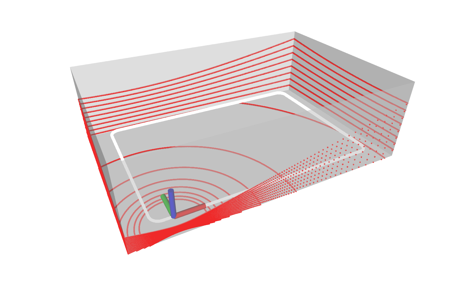
Figure 5: Simulation setup: A 16-channel lidar moves along a rectangular trajectory in a cuboid semi-closed space. The white line is the trajectory and the red lines are the laser points.

This study aims to verify the consistency of the proposed BA method. That is, whether the estimated covariance $\boldsymbol{\Sigma}_{\delta\mathbf{T}^{\star}}$ from (52) agrees with the ground-true covariance of the pose estimation error $\delta\mathbf{T}^{\star}$. As the ground-true covariance is unknown, we refer to a standard measure of consistency, the normalized estimation error squared (NEES) [57, 58], which is defined below:

$$\eta=(\delta\mathbf{T}^{\star})^{T}\boldsymbol{\Sigma}_{\delta\mathbf{T}^{\star}}^{-1}\delta\mathbf{T}^{\star},$$

where $\delta\mathbf{T}_{j}^{\star}$ is the estimation error of the pose defined according to (27):

$$\delta\mathbf{T}^{\star} \triangleq(\cdots,\delta\mathbf{T}_{j}^{\star},\cdots)\in\mathbb{R}^{6M_{p}},$$

$$\delta\mathbf{T}_{j}^{\star} =\begin{bmatrix}\text{Log}\left(\mathbf{R}_{j}^{\rm{gt}}\left(\mathbf{R}_{j}^{\star}\right)^{T}\right),&\mathbf{t}_{j}^{\rm{gt}}-\mathbf{R}_{j}^{\rm{gt}}(\mathbf{R}_{j}^{\star})^{T}\mathbf{t}^{\star}_{j}\end{bmatrix}^{T},$$

where the superscript “gt” denotes the ground-true poses and (${\mathbf{R}}_{j}^{\star}$, ${\mathbf{t}}_{j}^{\star}$) denotes the estimated pose for the $j$-th scan. Assume the pose estimate (${\mathbf{R}}_{j}^{\star}$, ${\mathbf{t}}_{j}^{\star}$) is unbiased (i.e., $E\left(\delta\mathbf{T}_{j}^{\star}\right)=\mathbf{0}$), if the computed covariance $\boldsymbol{\Sigma}_{\delta\mathbf{T}^{\star}}$ is the ground-truth, we can obtain the expectation

$$\!\!\!\!E(\eta)\!=\!E\!\left(\!(\delta\mathbf{T}^{\star})^{T}\boldsymbol{\Sigma}_{\delta\mathbf{T}^{\star}}^{-1}\delta\mathbf{T}^{\star}\right)\!=\!\text{trace}\!\left(\!E\!\left(\boldsymbol{\Sigma}_{\delta\mathbf{T}^{\star}}^{-1}\delta\mathbf{T}^{\star}(\delta\mathbf{T}^{\star})^{T}\right)\!\right)$$

$$\!=\!\text{trace}\!\left(\!\boldsymbol{\Sigma}_{\delta\mathbf{T}^{\star}}^{-1}E\!\left(\delta\mathbf{T}^{\star}(\delta\mathbf{T}^{\star})^{T}\right)\!\right)\!=\!\text{trace}(\mathbf{I})\!=\!\text{dim}(\delta\mathbf{T}^{\star}).$$ (53)

That is, if the solver is consistent, the expectation of NEES should be equal to the dimension of the optimization variable. If the expectation of NEES is far higher than the dimension, the estimator is over-confident (i.e., the computed covariance is less than the ground-truth). Conversely, it is conservative.

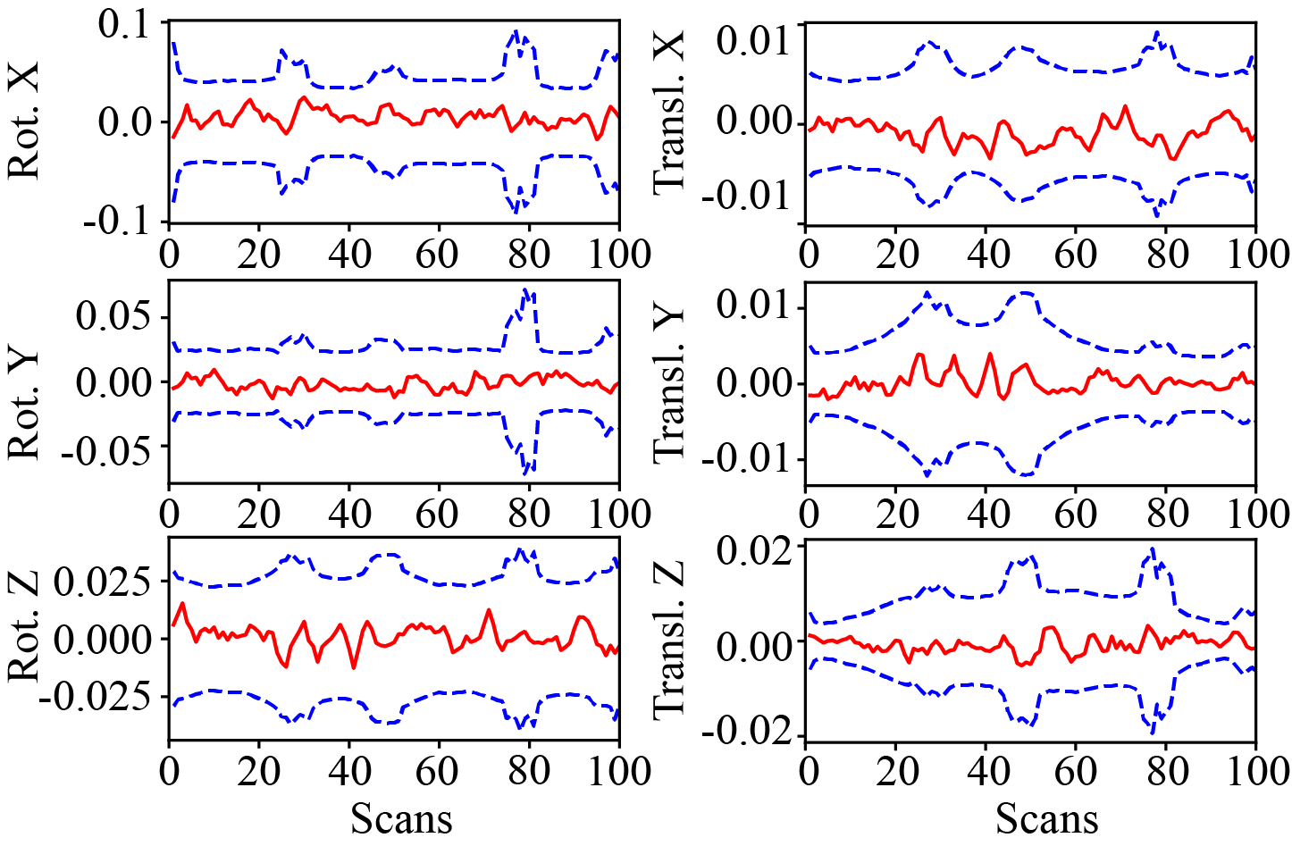
Figure 6: The error (red) of rotation (deg) and position (m) with $3\sigma$ bounds (blue) for one simulation run.

In practice, the expectation of NEES is evaluated by Monte Carlo method, where the NEES is computed for many runs and then averaged to produce the empirical expectation.

$$\bar{\eta}=\frac{1}{N}\sum_{i=1}^{N}\eta^{(i)}$$

where $\eta^{(i)}$ is the NEES computed at the $i$-th Monte Carlo run.

Figure 7: (a) The normalized NEES averaged over 100 Monte Carlo runs at different point noise levels. The NEES is normalized by the pose dimension (i.e., 600) for better visualization. (b) The rotation (red) and translation (blue) errors at different point noise levels. (c) The point cloud map with ground-true poses at noise levels $\sigma_{p}=$ 0.05m, 0.5m and 1m, respectively.

To conduct the Monte Carlo evaluation, we simulate a 16-channel lidar along a rectangular trajectory in a cuboid semi-closed space shown in Fig. 5. The size of the space is 30 m $\times$ 20 m $\times$ 8 m and the length of trajectory is about 92 m. 100 scans are equally sampled on the trajectory and the number of points in each scan is 28,800. To simulate realistic measurements, each point is corrupted with an independent isotropic Gaussian noise with multiple standard deviations $\sigma_{p}\in\{0.05,0.10,\cdots,1.00\}$ m and for each value of the standard deviation $\sigma_{p}$, we performed 100 Monte Carlo experiments, leading to a total number of 2000 experiments. In each run, we compute the optimal pose estimate from Algorithm 1 with the same parameters specified in Section IV and the covariance matrix from (52). The initial trajectory required in Algorithm 1 is obtained by perturbing the ground-true trajectory with a Gaussian noise with standard deviation $\delta\boldsymbol{\phi}=2$ deg and $\delta t=0.1$ m on each pose.To avoid unnecessary errors, we use the ground-true plane association across different scans and ignore the in-frame motion distortion in the simulation.

Fig. 6 shows orientation and position errors with the corresponding 3$\sigma$ bounds in one Monte Carlo experiment with $\sigma_{p}=0.05$ m. As can be seen, the pose estimation errors are very small and they all remain within the $3\sigma$ bounds very well, which suggests that our new method is consistent.

Furthermore, we test the consistency of our BA method under different levels of point noise, where the standard deviation of a point noise ranges from $\sigma_{p}=0.05$ m to $1$ m. The results are shown in Fig. 7(a) for the NEES averaged over 100 runs for each noise level and in Fig. 7(b) for the average pose error. For better visualization, the average NEES is normalized by the pose dimension (i.e., 600 for 100 poses on the trajectory) in Fig. 7(a). As can be seen, the normalized average NEES is very close to one, which suggests that our method is consistent, when the point noise is up to 0.3 m. Beyond this noise level, the first order approximation in (III-G) no longer holds, which undermines the accuracy of the computed covariance. We should note that this noise level rarely occurs in actual lidar sensors, which are well below 0.1 m. Moreover, from Fig. 7(b), we can see that our method produces accurate pose estimation even when the point noise are unrealistically large (up to 1 m, see Fig. 7(c) for the point cloud map at this point noise level).

VI Benchmark Evaluation

In this section, we compare our method with other multi-view registration methods for lidar point clouds. The experiment will be divided into two parts: Section VI-A evaluates all methods with known feature association on virtual point clouds, and Section VI-B evaluates the overall BA pipeline including both optimization solver and feature association on various real-world open datasets.

To verify the effectiveness of our method, we compare it with four state-of-the-art methods that focus on the lidar bundle adjustment (or similar) problem: Eigen-Factor (EF) [53], BALM [32], Plane Adjustment (PA) [49] and BAREG [54]. Among them, EF, BALM, BAREG are open sourced, so we use the available implementation on Github. PA is not available anywhere, so we re-implemented it in C++. To reduce the time cost of PA, we used the reduced Jacobian and residual technique in [47] (we derived it based on the cost function in Equation (10) of [49]), which avoids the enumeration of each individual point, and the Schur complement trick, which reduces the linear equation dimension at each optimization iteration. The re-implemented PA uses the same LM algorithm pipeline as in Algorithm 1 to make a fair comparison.

For the optimization solvers, our method and the re-implemented PA use the same parameters in Algorithm 1, while EF, BALM and BAREG use their default parameters as available on their open source implementation. All methods use the same termination condition shown in Sec. IV (i.e. maximal iteration number beow 50, rotation update below $10^{-6}$ rad, and translation update below $10^{-6}$ m), except for EF, which we found it converges too slowly and hence set the maximal iteration steps to 1000. In addition to the open source version of BALM (denoted by BALM), which samples only three points from each plane to lower the computation load, we also evaluated another vision (denoted by BALM-full) which keeps all the points on a plane and use the same default parameters as its open sourced version. All solvers use the same initial pose trajectories detailed later.

For the feature association, we use the same adaptive voxelization proposed in our previous work BALM [32], which registers all points in the world frame (using the initial trajectory) and recursively cuts the space into smaller voxels until the voxel contains a single feature that associates the points from multiple scans. EF did not address the feature association problem and PA did not open relevant association codes, so we use the method of BALM [32] too. BAREG used a adaptive voxelization method similar to BALM but has its own implementation, which we retain. All feature associations have the same set of parameters: the root voxel size $L$, the maximum voxelization layer $l_{\text{max}}$, the minimum number of points $n_{\text{min}}$ for a feature test, and the feature test thresholds $\gamma$. Exact values of these parameters are provided later.

Our proposed optimization method and the adaptive voxelization method in BALM [32] are applicable to both edge and plane features. However, we notice that in real-world point cloud data, edge features extracted based on local smoothness (e.g., [18]) are very noisy because the laser pulse emitted by lidars can barely hit an edge exactly due to the limited angular resolution. The situation is even worsened when the edge is at far or when the lidar has increased laser beam divergence, which creates many bleeding points behind an edge and degrades the edge points extraction [59]. As a consequence, we found that in practice, adding the edge features does not contribute much to the accuracy. Moreover, since the other methods, including EF, PA, and BAREG are only designed for plane features, for a fair comparison, we use only plane features in the following experiments for all methods. In fact, an edge is often created by an foreground object, which also makes a good plane feature, so dropping the edge feature does not reduce the number of constraints significantly.

VI-A Virtual point cloud

Figure 8: Convergence of different methods in BA optimization. (a) Cost convergence in one repeat experiment of the nominal settings $M_{f}=40$, $M_{p}=40$ and $N=40$ in one repeat experiment. (b) Iteration steps experienced by each method in all repeat experiments (i.e., 10) of all scenes (i.e., 13). The y-axis value represents how many experiments out of the total (130) has experienced the iteration number indicated on the x-axis.

To verify the effectiveness of the optimization solvers and their scalability to the number of pose $M_{p}$, number of feature $M_{f}$, and number of points $N$ per feature, we design a point-cloud generator which generates $M_{f}$ random planes and $M_{p}$ lidar scans at random poses. Each pose corresponds to one group of point-cloud whose number of points on each plane is $N$. Hence, there are totally $NM_{f}$ points at each scan. To mimic the real lidar point noises, we also corrupt the points sampled on each plane by a isotropic Gaussian noise with standard deviation $\sigma_{p}=0.05$m, the typical noise level for existing lidar sensors. In the nominal settings, $M_{f}=M_{p}=N=40$. From the nominal settings, we enumerate each of the three parameters at values $\{10,20,40,80,160\}$ to investigate the performance of each solver at different scales. This makes a total number of 13 scenes. In each scene, the experiment is repeated for 10 times with separately sampled poses, planes, and point noises, leading to a total 130 experiments. The initial pose trajectories for all the optimization methods are obtained by perturbing the ground-true poses by a Gaussian noise with standard deviation $\delta\boldsymbol{\phi}=2$ deg and $\delta t=0.1$ m.

VI-A1 Convergence

First we investigate the convergence performance of these methods. Fig. 8(a) shows the cost convergence for all methods in one repeat experiment of the nominal settings (i.e., $M_{f}=M_{p}=N=40$). Since different method uses different cost function, to compare them in one figure, the cost value of each method is normalized by its initial cost and then it is re-based such that the converged cost value of all methods are aligned at the same value. As can be seen, EF converes rather slowly and requires the most number of iterations. This is because EF uses a cost function similar to ours in (9), which is essentially a quadratic optimization, but uses only the gradient information for optimization. Indeed, slow convergence of the gradient descent method on a quadratic cost function is a very typical phenomenon [60]. PA and BAREG converge fast at the beginning but slowly when approaching the final convergence value. This is because PA optimizes both the plane parameters and scan poses, leading to a very large number of optimization variables that significantly slow down the speed at convergence. For BAREG, the empirical fixation of plane parameters also causes the optimization to slow down. In contrast, BALM, BALM-full and our method eliminates the plane parameters exactly and the resultant optimization problem is only in dimension of the pose number. Further leveraging the exact Hessian information in their optimization update, BALM, BALM-full and our method converge in four iterations, which represent the fastest convergence.

Fig. 8(b) shows the iteration experienced by each BA optimization method, where for each data point, the y-axis value represents how many experiments out of the total ($13\times 3=130$) experienced a certain iteration number indicated by the x-axis value. As can be seen, the overall trend agrees with the results in Fig. 8 (b) very well: our proposed method and BALM-full require only four or five iterations in all experiments, while BAREG and PA require up to 20 and 50 iterations, respectively. EF requires even more iterations beyond 50. The only exception is BALM, which experienced more iterations than BAREG in the worst case, the reason is that BALM samples only three points from each plane feature, which may reduce the robustness and increase the iteration steps in some cases.

VI-A2 Accuracy

Figure 9: Benchmark results on virtual point-cloud.

Fig. 9(a)-(f) shows the statistic values of the pose estimation accuracy in terms of RMSE. In each subplot, we fix two parameters of $M_{f},M_{p}$ and $N$ at the nominal values and change the third parameter to investigate the change of pose accuracy. Since the error of EF is much larger than the others, we used a broken y-axis to better display all the RMSE. As can be seen, the accuracy overall increases with the points per plane $N$ (in (b) and (e)) or number of plane features $M_{f}$ (in (c) and (f)), both increases the number of pose constraints. No such monotonic accuracy improvement is found in (a) and (d) as the pose number increases because increasing the pose number itself does not gives more pose constraints. Relatively speaking, our proposed method and BALM-full achieves the same highest accuracy, since they essentially optimizes the same cost using the same exact Hessian information. The next best methods are BAREG and PA. While optimizing the same point to plane distance with our method (and BALM-full), PA has significantly more optimization variables, which cause a much slower convergence where the solution is still slightly premature at the preset iteration number (i.e., 50). The next accurate method is BALM, which samples only three instead of all points (as in our method, BALM-full, BAREG and PA) and hence has higher RMSE. Finally, EF has the highest RMSE due to the very slow convergence, the solution is much premature even at the preset iteration number (i.e., 1000).

VI-A3 Computation time

Finally, we show the computation time of different solvers at different feature number $M_{f}$, pose number $M_{p}$, and point number $N$. The results are shown in Fig. 9(g)-(i), respectively. As can be seen, the time consumption of all methods increases with the number of poses $M_{p}$ (see (g)) and plane features $M_{f}$ (see (i)), which is reasonable since more poses or planes leads to a higher optimization dimension or more number of cost items, respectively. In contrast, as the point number $N$ increases, the method BALM-full increases rapidly since its time complexity involves $O(N^{2})$ while the rest methods (including ours) do not increase notably since they do not need to evaluate every raw point. Relatively speaking, our method achieves the lowest computation time in all cases due to the small number of iteration numbers and low time-complexity per iteration. The next efficient method is BAREG, which has very low time-complexity per iteration due to the empirical feature parameter fixation but significantly more iteration numbers due to the same reason. Compared with our method, PA has the same time complexity per iteration as discussed in Section III-F, but requires more iterations to converge. Hence its time cost is a little higher than ours and BAREG. BALM requires more iterations than our method and each iteration, it requires to enumerate the sampled three points. Collectively, it leads to a computation time higher than our method and also BAREG and PA. The slow convergence problem is more severe in EF, leading to an even higher computation time. Finally, the most time-consuming method is BALM-full, which, although has very small iteration numbers, takes significantly high time to compute the Hessian matrix in each iteration due to enumeration of each raw point.

VI-B Real-world datasets

TABLE II: Absolute trajectory error (RMSE,meters) for different methods.

Datasets	Sequence	ICP	GICP	NDT	EF	BALM	PA	BAREG	Ours
Hilti	Basement1	0.058	0.063	0.076	0.047	0.042	0.039	0.040	0.035
	Basement4	0.084	0.089	0.098	0.071	0.058	0.054	0.057	0.044
	Campus2	0.105	0.109	0.124	0.080	0.066	0.062	0.064	0.053
	Construction2	0.108	0.104	0.113	0.086	0.068	0.064	0.063	0.055
	LabSurvey2	0.066	0.069	0.072	0.054	0.025	0.021	0.023	0.018
	UzhArea2	0.182	0.191	0.211	0.161	0.131	0.125	0.127	0.117
VIRAL	eee01	0.159	0.163	0.172	0.122	0.073	0.057	0.061	0.038
	eee02	0.153	0.154	0.163	0.111	0.062	0.059	0.068	0.037
	eee03	0.171	0.175	0.180	0.127	0.082	0.078	0.072	0.052
	nya01	0.139	0.136	0.163	0.107	0.084	0.058	0.062	0.038
	nya02	0.160	0.159	0.124	0.114	0.067	0.059	0.061	0.047
	nya03	0.142	0.143	0.146	0.093	0.077	0.064	0.075	0.041
	sbs01	0.133	0.142	0.147	0.083	0.069	0.065	0.072	0.039
	sbs02	0.127	0.127	0.121	0.094	0.062	0.068	0.059	0.038
	sbs03	0.146	0.149	0.150	0.108	0.072	0.063	0.068	0.043
UrbanLoco	0117	1.382	1.364	1.372	0.728	0.625	0.577	0.596	0.495
	0317	1.384	1.299	1.289	0.914	0.691	0.689	0.715	0.648
	0426-1	1.436	1.457	1.566	1.014	0.875	0.765	0.733	0.689
	0426-2	1.676	1.693	1.543	1.113	0.924	0.894	0.917	0.822
Average		0.411	0.410	0.412	0.275	0.218	0.203	0.207	0.176

TABLE III: Occupied cells of point-cloud map for different methods.

Datasets	Sequence	ICP	GICP	NDT	EF	BALM	PA	BAREG	Our
		(inc.)	(inc.)	(inc.)	(inc.)	(inc.)	(inc.)	(inc.)	(base)
Hilti	Basement1	+20300	+20954	+21354	+16692	+6285	+4230	+5864	391962
	Basement4	+7826	+7283	+8178	+6683	+4762	+2628	+3752	558823
	Campus2	+14459	+15511	+21146	+8028	+2863	+2217	+2862	1319482
	Construction2	+6235	+9371	+10032	+6397	+1789	+1032	+986	979614
	LabSurvey2	+1680	+3141	+6331	+5043	+1375	+1176	+1228	139682
	UzhArea2	+9490	+9623	+10832	+6371	+2688	+1945	+2785	628951
VIRAL	eee01	+43185	+43439	+44578	+22731	+2564	+1028	+1321	1166482
	eee02	+10339	+14573	+15848	+6985	+5938	+4204	+5635	892368
	eee03	+8584	+9419	+7418	+5720	+2016	+1940	+1060	594921
	nya01	+53004	+56370	+48669	+26087	+7368	+4670	+4246	571365
	nya02	+38056	+37718	+38435	+24752	+4710	+3567	+3902	572960
	nya03	+14282	+13896	+16325	+10688	+5922	+2346	+2614	562583
	sbs01	+10069	+12196	+16597	+9635	+4224	+2348	+3691	794228
	sbs02	+16573	+16446	+21046	+10577	+9278	+7935	+5238	808235
	sbs03	+12257	+11154	+8974	+4682	+877	+682	+763	867174
UrbanLoco	0117	+46718	+47572	+50969	+16327	+7237	+3685	+5412	1743775
	0317	+37635	+33676	+41367	+20072	+13102	+6983	+8521	1709823
	0426-1	+9165	+10242	+13695	+9539	+2331	+1764	+1026	1632662
	0426-2	+31870	+30461	+29568	+13827	+3428	+2236	+4451	2176302
Average		+21617	+21002	+22703	+12146	+4671	+2979	+3439	953215

In this experiment, we conduct benchmark comparison on three real-world datasets. The first dataset is “Hilti” [61] which is a handheld SLAM dataset including indoor and outdoor environments. We use the lidar data collected by Ouster OS0-64 in the dataset. The ground-true lidar pose trajectory is captured by a total station or motion capture ssytem. The second dataset “VIRAL” [62] is collected on an unmanned aerial vehicle (UAV) equipped with two 16-channel OS1 lidars. One lidar is horizontal and the other is vertical. We will use the horizontal one in this experiment. It used a Leica Nova MS60 MultiStation to track a crystal prism on the UAV to provide ground-true positions. The last dataset “UrbanLoco” [63] is collected by a car driving on an urban streets. The lidar is Velodyne HDL 32E and the ground truth is given by the Novatel SPAN-CPT, a navigation system incorporating Real Time Kinematic (RTK) and precisional IMU measurements.

Two preprocessing are performed for all sequences: motion compensation and scan downsample. To compensate the points distortion caused by continuous lidar movements within a scan, we run a tightly-coupled lidar-inertial odometry, FAST-LIO2 [19], which estimates the IMU bias (and other state variables) and compensates the point motion distortion in real-time. We kept all points in a scan whose distortion has been compensated by FAST-LIO2 and discard the odometry output. The processed data are then downsampled from the original 10 Hz in all sequences to 2 Hz. This is because the BA methods need to process all scans at once, a 10Hz scan rate causes prohibitively high computation load for all BA methods. The downsampling is also similar to the keyframe selection in common SLAM frameworks.

We compare our method with EF, BALM, PA, and BAREG. Noticing that the computation time of BALM-full is prohibitively high due to the extremely large number of lidar points, we hence remove it from the benchmark comparison. For the rest methods, their solver parameters are kept the same for all sequences with values detailed before. For feature association, the parameters are $l_{\text{max}}=3,n_{\text{min}}=20,\gamma=\frac{1}{25}$. For the parameter $L$, it is set to $1$ m for “Hilti” and “VIRAL” and $2$ m for “UrbanLoco”.

In addition to the multi-view registration methods, we also compare with classic pairwise registration methods, including ICP, GICP, and NDT offered in PCL library. We run the pairwise registration methods in an incremental manner, where each new scan is registered and merged to the map incrementally. To constrain the computation time, in each new scan registration, only the last 20 scans are kept in the map. The pose estimation from the ICP is then used as the initial trajectory for the feature association and optimization of the BA methods, including EF, BALM, PA, BAREG, and ours.

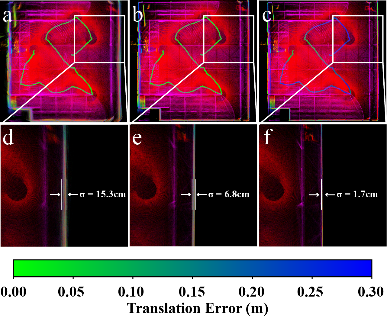
Figure 10: Point cloud map of the UzhArea2 sequence in “Hilti”. (a) registered by ground-true pose trajectory. (b) registered by ground-true position with rotation optimized by our BA method. (c) registered by poses fully optimized by our BA method. (d), (e) and (f) points on one side wall in (a), (b) and (c), respectively.

VI-B1 Accuracy

Table II shows the ATE results. As can be seen, our method consistently achieves the best results in all 19 sequences. The next accurate method is PA and BAREG, followed by BALM and EF. This trend is in great agreement with the results on virtual point-cloud shown in Section VI-A-2 with explanations detailed therein. In particular, our method achieves an accuracy within a few centimeters in all sequences of “Hilti” and “VIRAL”, with only one exception (i.e., UzhArea2), which will be analyzed later. The centimeter level accuracy achieved by our method is at the same level of lidar point noises. Moreover, using only lidar measurements, our method achieved an average accuracy of $4.2$ cm on all VIRAL dataset sequences, which outperforms the accuracy $4.7$ cm reported in VIRAL-SLAM [62] that fuses all data from stereo camera, IMU, lidar, and UWB. The accuracy on “UrbanLoco” is lower (analyzed later) than other datasets, but still outperforms the other BA methods. Finally, we can notice that the BA methods (i.e., EF, BALM, PA, BAREG and ours) generally outperforms the pairwise registration methods (i.e., ICP, GICP and NDT) due to the full consideration of multi-view constraints.

Now we investigate the performance degradation on “UrbanLoco” and the sequence UzhArea2 in “Hilti” more closely. For the “UrbanLoco” dataset, we found that the RTK ground-truth had some false sudden jumps, which contributes the large ATEs. This sudden jump may be caused by tall buildings in the crowded urban area which lowers the quality of the ground-truth. For the sequence UzhArea2, we register the point cloud with the ground-true pose trajectory and compare it with the point cloud registered with our BA method in Fig. 10. As can be seen, with the ground-true pose, points on the side wall are very blurry and points on the wall form a plane with standard deviation up to 15.3 cm (Fig. 10(d)); with the ground-true translation but with rotations optimized by our BA method, the points on the side wall are much more ordered and form an apparent plane of standard deviation 6.8 cm (Fig. 10(e)); with poses fully optimized by our method, the points are even more consistent and the standard deviation is 1.7 cm (Fig. 10(f)). From these results, we suspect that the ground-truth may be affected by some unknown errors (e.g., marker position change during the data collection). Indeed, we found similar problem on this sequence also occurred in other works [64]. Moreover, the standard deviation of 1.7cm achieved by our method is exactly the ranging accuracy of the lidar sensor, which confirms that our method achieves a mapping accuracy at the noise level of raw points as if the sensor motion had not occurred.

VI-B2 Mapping quality

A significant advantage of the BA method is the direct optimization of the map accuracy. To evaluate the map quality without a ground-true map, we adopt a method proposed by Anton et al. [65]. The method cuts the space into small cells and then counts the number of cells that lidar points occupy. The less the occupied cells, the higher the map quality. This indicator is intuitive: if points from different scans are registered accurately, they should agree with each other to the best extent, hence occupying the minimum possible number of cells. Based on this method, Table III presents the number of occupied cell with size 0.1 m. To better show the difference among different methods, the number of occupied cells are subtracted by our method for each sequence. We show the number of occupied cells by our method and the difference value of other methods. As can be seen, our method consistently achieved the best performance in all sequences and the next best is PA and BAREG. This trend also agrees with the ATE results very well.

VI-B3 Computation time

Finally, we compare the computation time. Since the pairwise registration methods, including ICP, GICP, and NDT, perform repetitive incremental registration at each scan reception, its computation time is very different from the BA methods that perform batch optimization on all scans at once. Therefore, we only compare the computation time of BA methods. Table IV shows the total computation time of optimization. As can be seen, our method consumes the least computation time, about one sixth of the BAREG, one eighth of PA, one tenth of BALM, and one seventieth of EF. The overall trend agree with the results on vitual point cloud in Section VI-A-3 with explanations detailed therein.

TABLE IV: Optimization time cost for different methods

Sequence	EF	BALM	PA	BAREG	Our
Hilti
Basement1	1196.29	150.97	101.93	89.01	14.60
Basement4	1335.38	171.22	130.09	123.71	17.60
Campus2	1682.41	331.87	274.36	182.50	27.75
Construction2	2987.39	392.71	309.20	230.33	37.24
LabSurvey2	228.47	38.56	32.47	25.30	4.95
UzhArea2	139.47	18.67	13.51	12.13	3.60
VIRAL
eee01	2419.48	269.81	217.85	179.67	25.62
eee02	1472.02	180.29	137.20	107.29	17.74
eee03	460.28	73.54	56.34	43.32	6.93
nya01	2642.51	388.54	344.50	259.87	41.98
nya02	3286.82	481.57	392.57	275.92	48.86
nya03	3860.17	507.03	469.02	285.93	47.51
sbs01	2310.04	296.99	246.44	182.54	29.33
sbs02	2321.43	290.75	240.55	193.18	33.30
sbs03	2193.25	384.63	352.39	242.30	39.22
Urbanloco
0117	631.52	80.41	57.49	50.57	7.09
0317	703.25	88.20	78.75	52.83	9.25
0426-1	149.97	37.75	21.87	17.04	5.30
0426-2	842.18	137.04	104.15	80.43	8.62
Average	1634.88	227.39	188.41	138.62	22.42

VII Applications

Bundle adjustment is the central technique of many lidar-based applications. In this section, we show how our bundle adjustment method can effectively improve the accuracy or computation efficiency of three vital applications: lidar-inertial odometry, multi-lidar calibration, and global mapping.

VII-A Lidar-inertial odometry with sliding window optimization

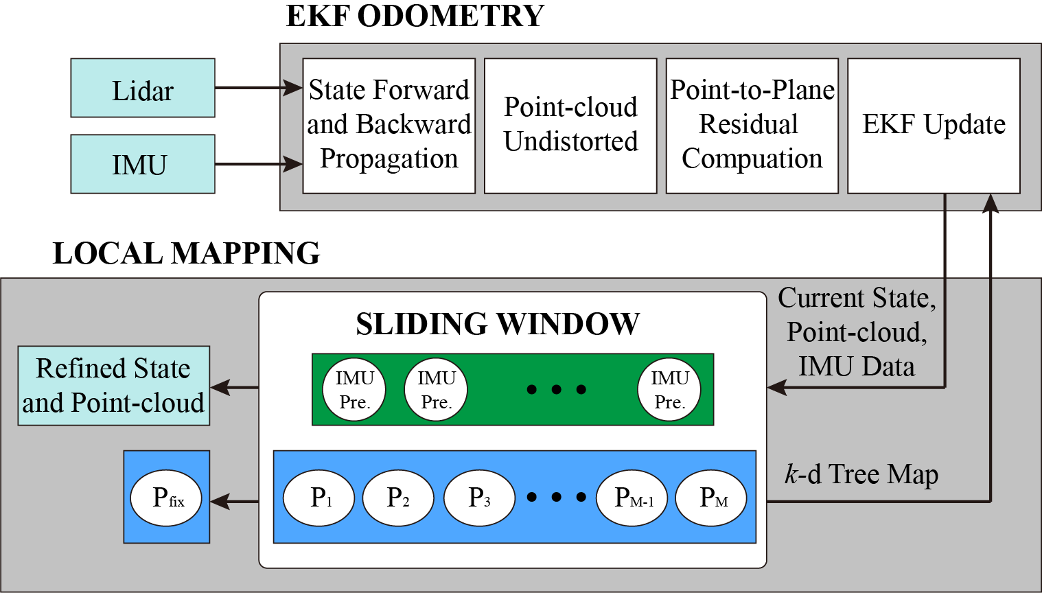
Figure 11: Overview of the LIO system with BA and IMU preintegration

TABLE V: ATE and time cost per scan of FAST-LIO2 and LIO with BA

	ATE (m)		Time (ms)
	FAST-LIO2	Local-BA	FAST-LIO2	Local-BA
				(Odom/BA Opt.)
utbm8	23.7	20.4	22.05	31.73/92.11
utbm9	45.9	39.1	25.44	33.42/95.43
utbm10	16.8	13.1	22.48	30.46/97.81
uclk4	1.31	1.15	20.14	19.53/69.89
nclt4	8.50	9.23	15.72	21.77/59.83
nclt5	6.65	6.25	16.60	26.13/61.23
nclt6	20.57	20.34	15.84	25.14/63.19
nclt7	6.58	5.69	16.87	23.18/62.53
nclt8	30.08	26.24	14.25	24.80/69.29
nclt9	5.56	5.07	13.65	22.98/67.36
nclt10	16.29	14.10	21.79	23.41/64.45
Average	16.54	14.61	18.62	25.68/73.01

A local bundle adjustment in a sliding window of keyframes has been widely used in visual odometry and proved to be very effective in lowering the odometry drift [66, 67, 26, 27]. Similar idea could apply to the lidar-inertial odometry based on our BA method. To demonstrate the effectiveness, we design a lidar-inertial odometry system as shown in Fig. 11. The system is divided into two parts: the EKF-based front-end, which provides initial yet timely pose estimation (EKF odometry), and the BA-based back-end, which refines the pose estimation in a sliding window (Local mapping). The EKF design is similar to FAST-LIO2 [19] which compensates the motion distortion in the incoming lidar scans and performs EKF propagation and update on the state manifold. The sliding window optimization performs a local BA among the most recent 20 scans considering constraints of IMU preintegration [58] and constraints from plane features co-visible among all scans in the window (Section III). After the convergence of the local BA, points in the local window are built into a $k$-d tree to register the next incoming scan. Furthermore, the oldest scan is removed from window and its contained points are merged into the global point cloud map.

We compare our proposed system with one state-of-art lidar-inertial odometry, FAST-LIO2 [19], which performs incremental pairwise scan registration via GICP. The comparison is conducted on “utbm” , “uclk”, and “nclt” dataset that evaluated by FAST-LIO2, so the results of FAST-LIO2 are directly read from the original paper [68]. As can be seen in Table V, benefiting from the abundant multi-view constraints in the local sliding window, our system consistently outperforms FAST-LIO2 in terms of accuracy with considerable margins except the sequence “nclt4”. The improvements in odometry accuracy confirm the effectiveness of the local BA optimization. The improvement in accuracy comes with increased computation costs as shown in the last two columns of Table V, where for FAST-LIO2, we record the time of each scan-to-map registration and for our LIO system, the time consumption is divided into two parts: one is the front-end scan-to-local map registration and the back-end local BA optimization. As can be seen, our system has a little more time consumption in front-end than FAST-LIO2 because of the building of a $k$-d tree, which takes a constant time overhead, while FAST-LIO2 uses a more efficient incremental $k$-d tree structure. In addition, our system requires an average of 73 ms in the back-end local BA optimization, which ensures a 10 Hz running frequency for both the front-end and back-end. Since the back-end runs in parallel in a separate thread, the overall odometry latency of our system is only 7 ms more than that of FAST-LIO2.

VII-B Multiple-lidar Calibration

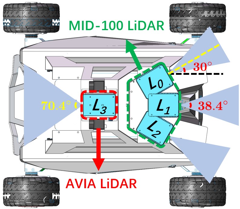
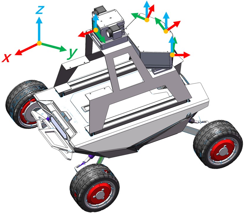
Figure 12: The customized multi-sensor vehicle platform in [69]. The MID-100 lidar consists of three lidars: $L_{0}$, $L_{1}$ and $L_{2}$, with FoV overlap between adjacent lidars 8.4^∘. The AVIA lidar is denoted as $L_{3}$. (a) The FoV coverage of each lidar sensor. (b) Each lidar sensor’s orientation denoted in the right-handed coordinate system.

With the ability of concurrent optimization of multiple lidar poses, our BA method can be applied to multi-lidar extrinsic calibration. We consider the problem in [69], which aims to calibrate the extrinsic of multiple solid-state lidars shown in Fig. 12. Due to the very small FoV, these lidars have very small or even no FoV overlap. To create co-visible features, the vehicle is rotated for one cycle, during which a set of point cloud scans are collected by all lidars. Due to the rotation, it further introduces unknown lidar poses, in addition to the extrinsic, to estimate.

To formulate the simultaneous localization and extrinsic calibration problem, we choose a reference lidar as the base and calibrate the extrinsic of the rest lidars relative to it. Denote $\prescript{G}{R}{\mathbf{T}_{j}},j=1,\cdots,M_{p}$, the pose of the reference lidar at $j$-th scan in a rotation, $\prescript{R}{L_{k}}{\mathbf{T}}$ the extrinsic of the $k$-th lidar relative to the base lidar. Then, following  (25), the cost item corresponding to the $i$-th plane feature is

$$\begin{split}&c_{i}(\prescript{G}{R}{\mathbf{T}_{j}},\prescript{R}{L_{k}}{\mathbf{T}})=\lambda_{3}\left({\mathbf{A}\left({\sum_{j=1}^{M_{p}}\prescript{G}{R}{\mathbf{T}_{j}}\cdot\mathbf{C}_{f_{ij}}^{r}\cdot\prescript{G}{R}{\mathbf{T}_{j}^{T}}}\right.}\right.\\ &\qquad\left.{\left.{+\sum_{k\neq r}\prescript{G}{R}{\mathbf{T}_{j}}\cdot\prescript{R}{L_{k}}{\mathbf{T}}\cdot\mathbf{C}_{f_{ij}}^{k}\cdot\left(\prescript{G}{R}{\mathbf{T}_{j}}\cdot\prescript{R}{L_{k}}{\mathbf{T}}\right)^{T}}\right)}\right)\end{split}$$ (54)

where $\mathbf{C}_{f_{ij}}^{r},\mathbf{C}_{f_{ij}}^{k}$ are the point cluster of the reference lidar and the $k$-th lidar, respectively, observed on the $i$-th feature at the $j$-th scan. Following Theorem 4, the first and second order derivatives of (54) can be obtained by chain rules, whose details are omitted here due to limited space.

We demonstrate the advantage of the proposed BA approach in multi-lidar calibration with the latest state-of-the-art calibration methods based on ICP [22] and BALM [69]. The ICP-based method [22] optimizes the extrinsic parameter $\prescript{R}{L_{k}}{\mathbf{T}}$ and base lidar pose $\prescript{G}{R}{\mathbf{T}_{j}}$ by repeatedly registering the point cloud by each lidar at each scan to the rest lidar points until convergence, whereas in both BALM-based method [69] and our method, the extrinsic parameter $\prescript{R}{L_{k}}{\mathbf{T}}$ and base lidar pose $\prescript{G}{R}{\mathbf{T}_{j}}$ are optimized concurrently. In [22] the feature correspondence searching is conducted by a $k$-d tree data structure, while in [69] and our method, this is resolved by adaptive voxelization proposed in BALM [32]. To restrain the computation time, the point number in each voxel of [69] have been down-sampled to four, whereas in our method, all feature points are used.

We test these methods on two lidar setups in the system shown in Fig. 12: lidars with small field-of-view (FoV) overlap (MID-100 self calibration) and lidars without FoV overlap (AVIA and MID-100 calibration). Since the extrinsic between the internal lidars of MID-100 (i.e., $\prescript{L_{1}}{L_{0}}{\mathbf{T}}$, $\prescript{L_{1}}{L_{2}}{\mathbf{T}}$) is known fromt he manufacturer’s in-factory calibration, it is thus served as the ground truth in both setups. Moreover, in the MID-100 self calibration setup, the middle $L_{1}$ is chosen as the reference lidar to calibrate the extrinsic of adjacent lidars, i.e., $\prescript{L_{1}}{L_{0}}{\mathbf{T}}$, $\prescript{L_{1}}{L_{2}}{\mathbf{T}}$. This lidar setup is tested with data collected in both [22] and [69] under two scenes which contributes to eight calibration results. In the MID-100 and AVIA calibration setup, the $L_{3}$ is selected as the reference lidar to calibrate the extrinsic of each internal lidar of MID-100, i.e., $\prescript{L_{3}}{L_{0}}{\mathbf{T}}$, $\prescript{L_{3}}{L_{1}}{\mathbf{T}}$ and $\prescript{L_{3}}{L_{2}}{\mathbf{T}}$. We then calculate the relative pose $\prescript{L_{1}}{L_{0}}{\mathbf{T}}$, $\prescript{L_{1}}{L_{2}}{\mathbf{T}}$ from the calibrated results and compare them with the ground truth. This lidar setup is tested with data collected under two scenes in [69] since no AVIA lidar was used in [22], which contributes another four calibration results.

The total twelve independent calibration results are illustrated in Fig. 13 and Fig. 14. It is seen the our proposed method outperforms the ICP-based method [22] especially in translation. This is due to the concurrent optimization of all poses and extrinsic at the same time, which leads to full convergences within a few iterations. In contrast, the repetitive pairwise ICP registration leads to very slow convergence. The optimization did not fully converge after the maximum iteration number (max_iter=40), a phenomenon detailed in [69]. Furthermore, since all raw points on a feature are utilized in our method, the accuracy of our proposed work is also slightly improved when compared with the BALM-based method [69], which sample a few points on a feature to restrain the computation time. The averaged time consumption in each step of these methods have been summarized in Table VI. It is seen our proposed work and [69] has significantly shortened the calibration time in each step compared with the ICP-based method. This is due to the use of adaptive voxelization which saves a great amount of time in $k$-d tree build and nearest neighbor search used in [22]. Compared with [69], our proposed BA has further increased the computation speed due to the use of point cluster technique avoiding the enumerating of individual points in the BALM-based method [69].

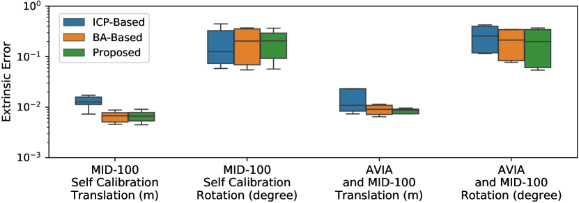
Figure 13: Extrinsic calibration results of the ICP-based [22], BALM-based [69] and our proposed method in two experiment setups (with small or without FoV overlap).

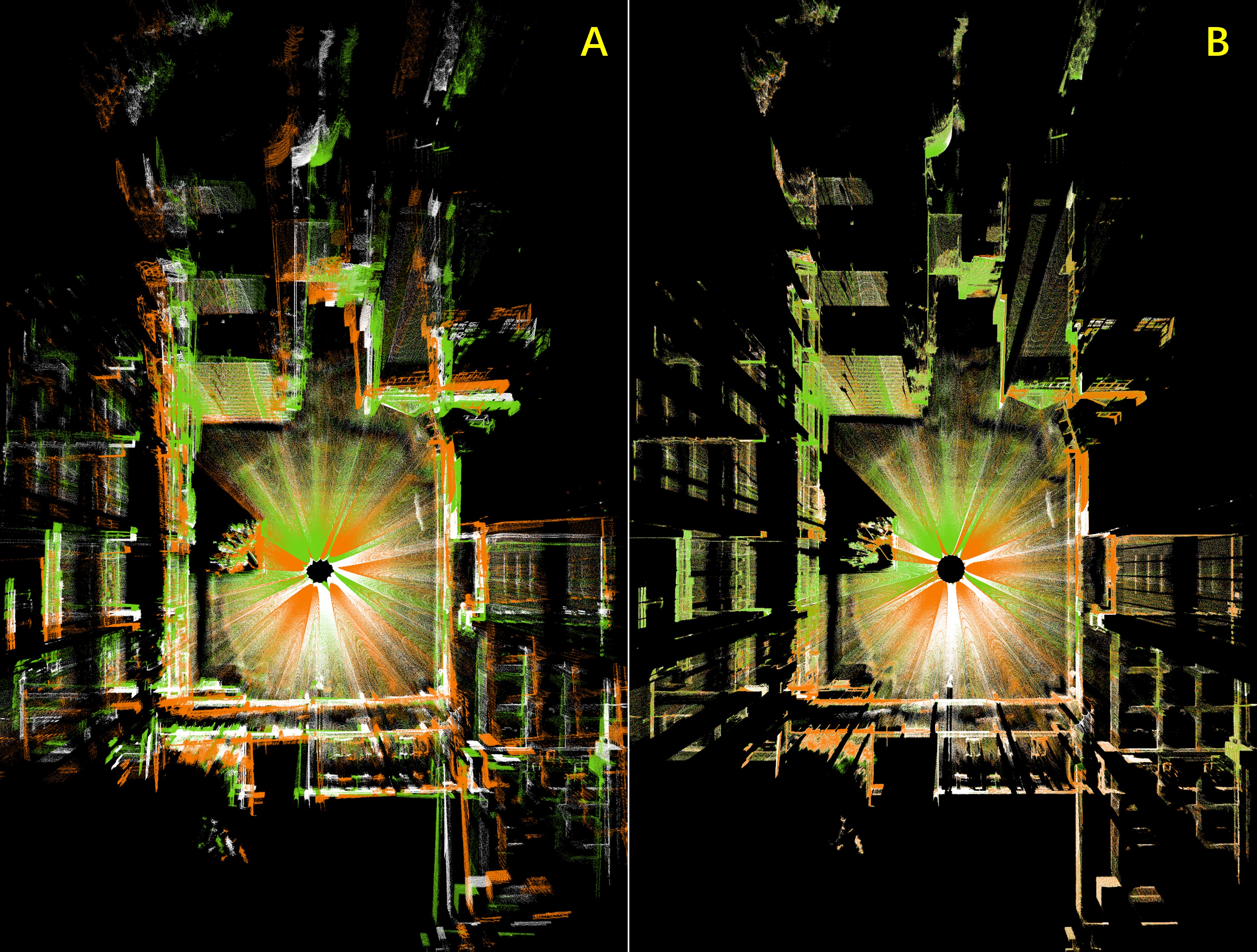
Figure 14: The point cloud of MID-100 lidar in Scene-1 reconstructed before (A) and after (B) extrinsic optimization. The base lidar ($L_{1}$) point cloud is colored in white and the two lidars to be calibrated ($L_{0}$, $L_{2}$) are colored in orange and green, respectively.

TABLE VI: Average time (second) per iteration for multi-lidar calibration

	Pose	Extrinsic	Joint
Method	Optimization	Optimization	Optimization
ICP-Based [22]	5.16	6.10	14.98
BALM-Based [69]	0.23	0.58	3.09
Proposed	0.19	0.20	0.80

VII-C Global BA on Large-Scale Dataset

In this section, we show that our proposed BA method could also be used to globally refine the quality of a large-scale lidar point cloud. It is becoming popular to use pose graph optimization (PGO) as the back-end to enhance the overall lidar odometry precision in SLAM system [70]. The optimal poses are obtained by minimizing the summed error between the relative transformation of these poses and that estimated in the front-end odometry. One drawback of the PGO is that it cannot reinforce the map quality directly. A divergence in point cloud mapping would occur if the estimation of the relative poses near the loop is ill. We show that the mapping quality (and odometry accuracy) could be further improved with our BA method even after PGO is performed.

We choose to validate on three sequences from the KITTI dataset [71]. The initial lidar odometry is provided by the state-of-the-art SLAM algorithm MULLS [70] with loop closure function enabled. We directly feed this odometry to our BA algorithm and concurrently optimize the entire poses. The optimization results (RMSE of the odometry error) are summarized in Table VII. It is seen that even with loop closure function, some divergence still exist in the area near the loop of the point cloud due to ill estimations. With our proposed global BA refinement, the accuracy in odometry is further improved and the divergence in point cloud is eliminated (see closeup in Fig. 15).

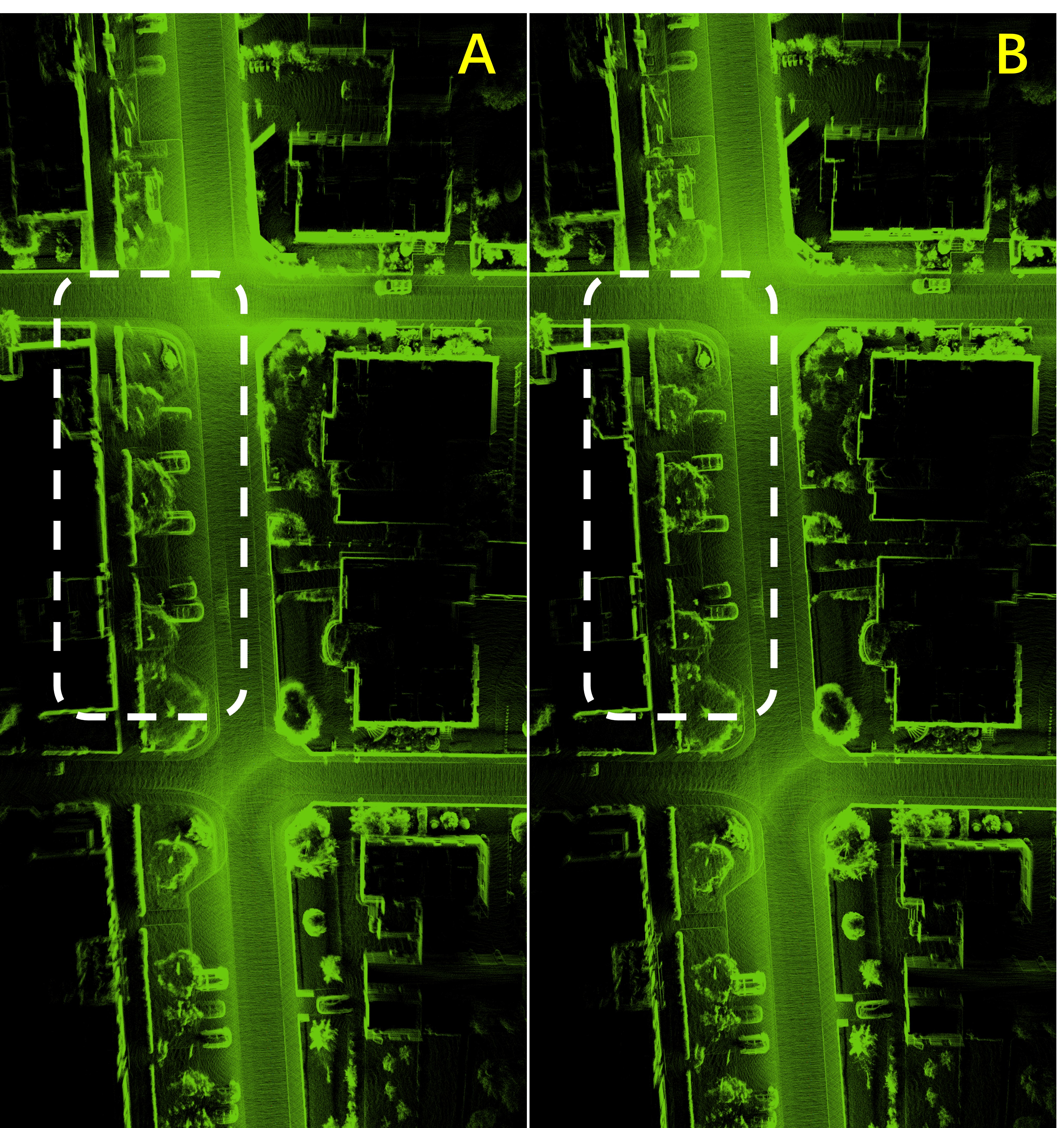
(a) Sequence 05

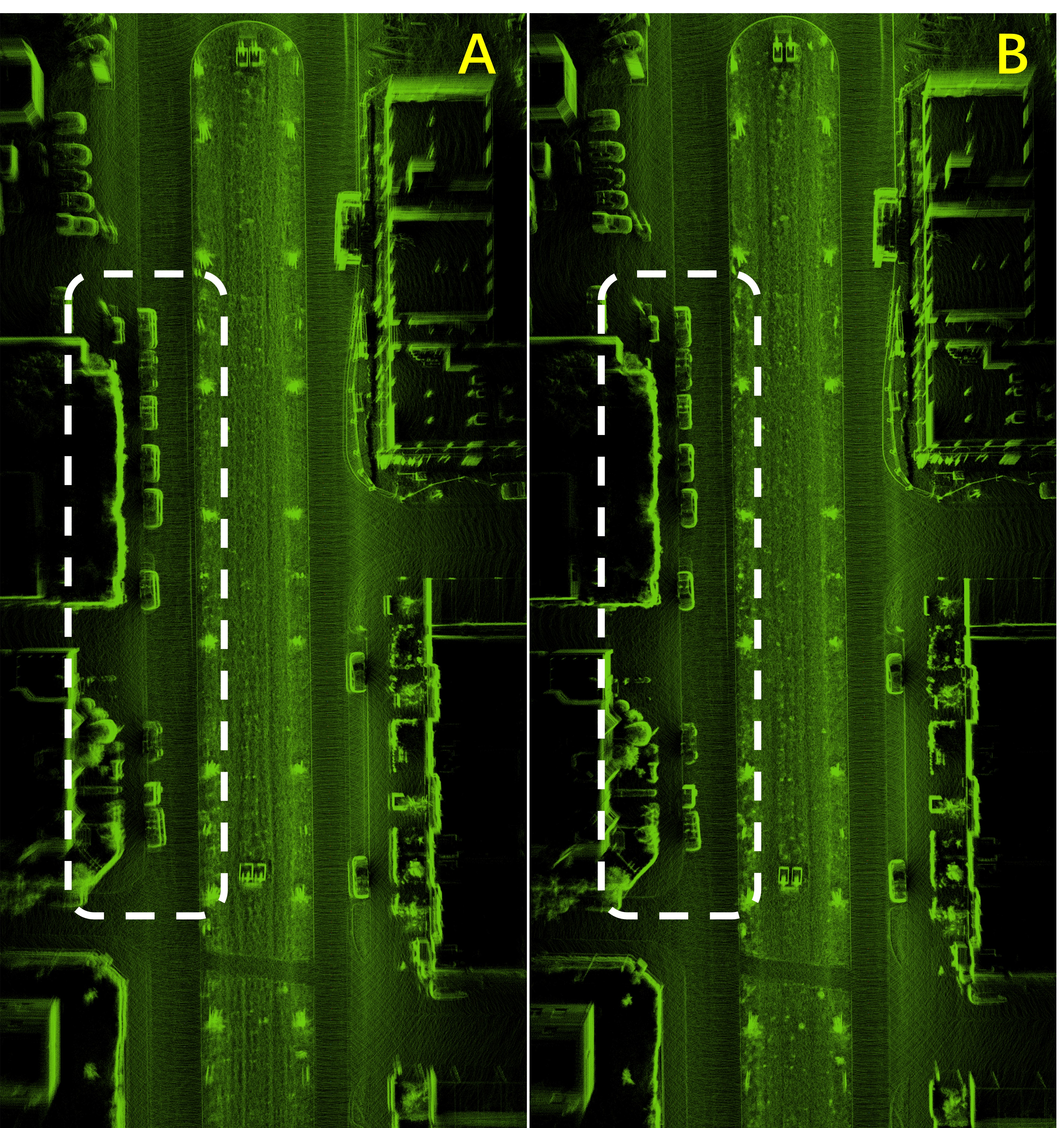
(b) Sequence 06

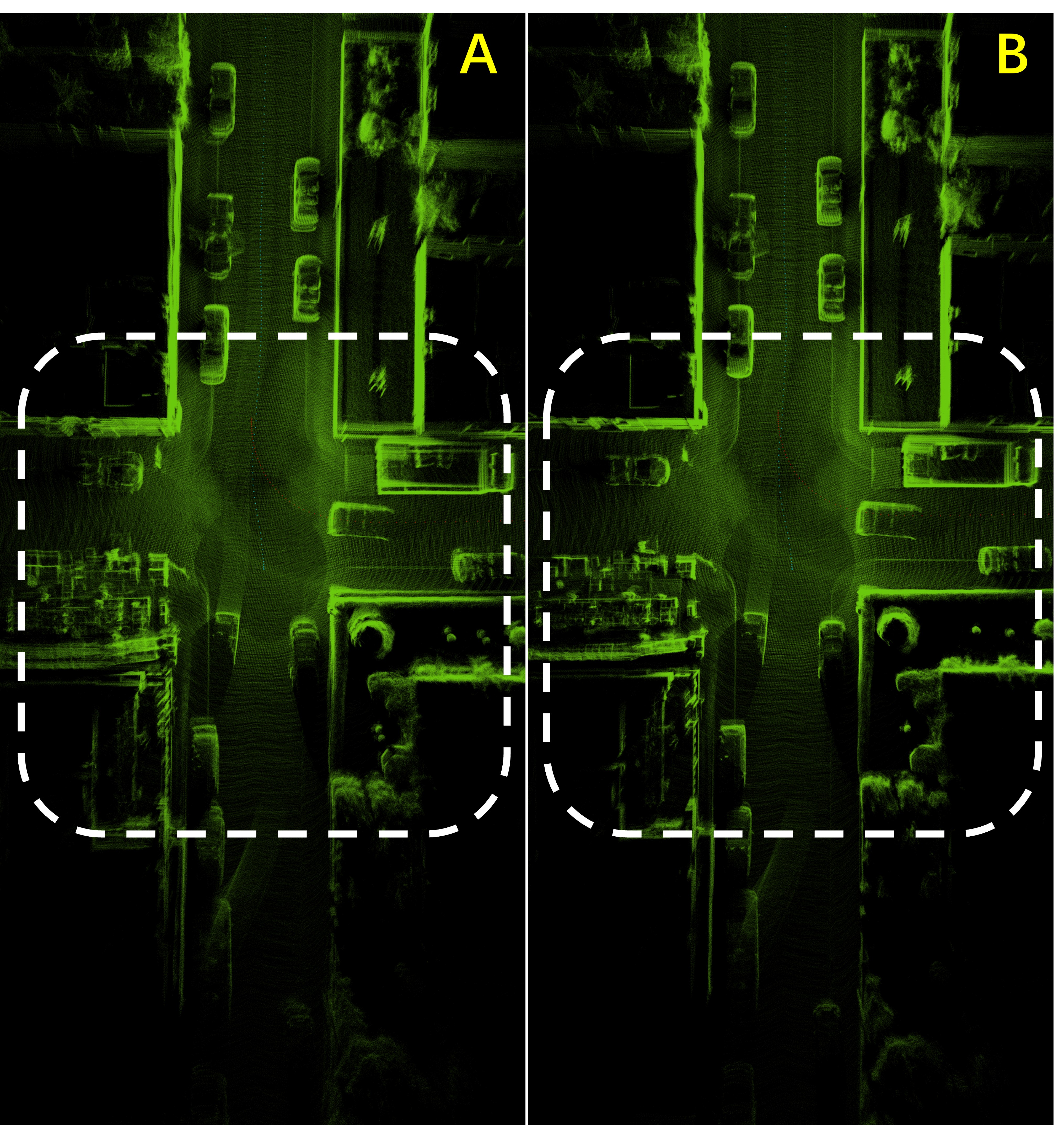
(c) Sequence 07

Figure 15: Comparison of odometry accuracy on KITTI dataset [71]. The left image (A) of each subplot depicts the point cloud reconstructed by MULLS [70] which is used as our initial value. The right image (B) of each subplot is the point cloud optimized by our proposed global BA method. The white dashed rectangle emphasized the difference (zoomed view is recommended).

TABLE VII: ATE (meters) for KITTI datasets

Method	Seq. 05	Seq. 06	Seq. 07
MULLS [70]	0.97	0.31	0.44
Proposed	0.65	0.27	0.33

VIII Discussion

Here we discuss the efficiency, accuracy, and extendability of the proposed bundle adjustment method.

VIII-A Efficiency

Our method achieved lower computation time than other state-of-the-art counterparts. The efficiency of our method are attributed to three inter-related and rigorously-proved techniques that make fully use of the problem nature and lidar point cloud property. The first technique is the solving of feature parameters in a closed-form before the BA optimization. It allows the feature parameters to be removed from the optimization, which fundamentally reduces the optimization dimension to the dimension of the pose only, a phenomenon that did not exist before in visual bundle adjustment problem. The second technique is a second-order solver which fits the quadratic cost function naturally and leads to fast convergence in the iterative optimization. This is enabled by the analytical derivation of the closed-form Jacobian and Hessian matrices of the cost function. The third technique is the point cluster, which enables the aggregation of all raw points without enumerating each individual point in neither of the cost evaluation, derivatives evaluation, or uncertainty evaluation. Collectively, these three techniques lead to an BA optimization with much lower dimension and a time complexity of $O(M_{f}M_{p}+M_{f}M_{p}^{2}+M_{p}^{3})$ in each iteration, which achieves the lowest time consumption when compared with other second order methods (e.g., BALM [32] and plane adjustment [47]).

VIII-B Accuracy

Benefiting from the point cluster technique, our proposed method is able to exploit the information of all raw point measurements, achieving high pose estimation accuracy (a few centimeters) at the level of lidar measurement noise. Optimization from the raw lidar points also enables the developed method to estimate the uncertainty level of the estimated pose, which may be useful when this information is further fused with measurements from other sensors (e.g., IMU sensors). Moreover, by minimizing the Euclidean distance from each raw point to the corresponding feature, our method can reinforce the map consistency in a more direct manner than conventional pose graph optimization. While at a higher computation cost (due to the more complete consideration of features co-visible in multiple scans), it considerably improves the mapping accuracy which is important for mapping applications. Due to this reason, our method is particularly useful for accuracy refinements from a baseline pose trajectory that can be obtained by an odometry or a pose graph optimization module. The second order optimization provides very fast convergence when the solution is near to the optimal value, preventing premature solutions.

VIII-C Extendability

As a basic technique for multiple scan registration, our proposed method can be easily be integrated with other formality of data, such as images and IMU measurements, by incorporating visual bundle adjustment factors and IMU pre-integration factors [58] in the optimization. Moreover, besides the frame-based pose trajectory, which attaches each frame an independent pose to estimate, our method can also work with other forms of pose trajectories, such as continuous-time trajectories based on Splines [9, 72] or Gaussian Process models [73, 74], which have the capability to compensate the in-frame motion distortion. According to the chain rules, the derivatives of the BA cost with respect to the trajectory parameters will consist of two parts: the first is the derivative of the BA cost with respect to the pose of each point cluster as derived in this paper, and the second part is the derivatives of the pose with respect to the trajectory parameters, which depends on the specific trajectories being used.

IX Conclusion

This paper proposed a novel bundle adjustment method for lidar point cloud. The central of the proposed method is a point cluster technique, which aggregates all raw points into a compact set of parameters without enumerating each individual point. The paper showed how the bundle adjustment problem can be represented by the point cluster and also derived the analytical form of the Jacobian and Hessian matrices based on the point cluster. Based on these derivations, the paper developed a second-order solver, which estimates both the pose and the pose uncertainty. The developed BA method is open sourced to benefit the community.

Besides the technical developments, this paper also made some theoretical contributions, including the formalization of the point cluster and its operations, revealing of the invariance property of the formulated BA optimization, the proof of null space and sparsity of the derived Jacobian and Hessan matrices, and the time complexity analysis of the proposed BA method and its comparison with others. These theoretical results serve the foundation of our developed BA techniques.

The proposed methods and implementations were extensively verified in both simulation and real-world experiments, in terms of consistency, efficiency, accuracy, and robustness. In all evaluations, the proposed method achieved consistently higher accuracy while consuming significantly lower computation time. This paper further demonstrated three applications of the BA techniques, including lidar-inertial odometry, multi-lidar calibration, and high-accuracy mapping. In all applications, the adoption of BA method could effectively improve the accuracy or the efficiency.

In the future, we would like to incorporate the BA method more tightly to the above applications and beyond. This would require more thorough considerations of many practical issues, such as point cloud motion compensation, removal of dynamic objects, tightly-fusion with other formality of sensor data (e.g., IMU, camera) and module (e.g., loop closure).

See pages 1- of supp.pdf

References

- [1] S. Thrun, M. Montemerlo, H. Dahlkamp, D. Stavens, A. Aron, J. Diebel, P. Fong, J. Gale, M. Halpenny, G. Hoffmann et al., “Stanley: The robot that won the darpa grand challenge,” Journal of field Robotics, vol. 23, no. 9, pp. 661–692, 2006.
- [2] C. Urmson, J. Anhalt, D. Bagnell, C. Baker, R. Bittner, M. Clark, J. Dolan, D. Duggins, T. Galatali, C. Geyer et al., “Autonomous driving in urban environments: Boss and the urban challenge,” Journal of field Robotics, vol. 25, no. 8, pp. 425–466, 2008.
- [3] J. Levinson, J. Askeland, J. Becker, J. Dolson, D. Held, S. Kammel, J. Z. Kolter, D. Langer, O. Pink, V. Pratt et al., “Towards fully autonomous driving: Systems and algorithms,” in 2011 IEEE intelligent vehicles symposium (IV). IEEE, 2011, pp. 163–168.
- [4] Y. Li and J. Ibanez-Guzman, “Lidar for autonomous driving: The principles, challenges, and trends for automotive lidar and perception systems,” IEEE Signal Processing Magazine, vol. 37, no. 4, pp. 50–61, 2020.
- [5] F. Gao, W. Wu, W. Gao, and S. Shen, “Flying on point clouds: Online trajectory generation and autonomous navigation for quadrotors in cluttered environments,” Journal of Field Robotics, vol. 36, no. 4, pp. 710–733, 2019.
- [6] F. Kong, W. Xu, Y. Cai, and F. Zhang, “Avoiding dynamic small obstacles with onboard sensing and computation on aerial robots,” IEEE Robotics and Automation Letters, vol. 6, no. 4, pp. 7869–7876, 2021.
- [7] Y. Ren, F. Zhu, W. Liu, Z. Wang, Y. Lin, F. Gao, and F. Zhang, “Bubble planner: Planning high-speed smooth quadrotor trajectories using receding corridors,” arXiv preprint arXiv:2202.12177, 2022.
- [8] B. Schwarz, “Mapping the world in 3d,” Nature Photonics, vol. 4, no. 7, pp. 429–430, 2010.
- [9] M. Bosse, R. Zlot, and P. Flick, “Zebedee: Design of a spring-mounted 3-d range sensor with application to mobile mapping,” IEEE Transactions on Robotics, vol. 28, no. 5, pp. 1104–1119, 2012.
- [10] M. Helmberger, K. Morin, B. Berner, N. Kumar, G. Cioffi, and D. Scaramuzza, “The hilti slam challenge dataset,” IEEE Robotics and Automation Letters, 2022.
- [11] D. Wang, C. Watkins, and H. Xie, “Mems mirrors for lidar: a review,” Micromachines, vol. 11, no. 5, p. 456, 2020.
- [12] Z. Liu, F. Zhang, and X. Hong, “Low-cost retina-like robotic lidars based on incommensurable scanning,” IEEE/ASME Transactions on Mechatronics, vol. 27, no. 1, pp. 58–68, 2021.
- [13] P. J. Besl and N. D. McKay, “Method for registration of 3-d shapes,” in Sensor fusion IV: control paradigms and data structures, vol. 1611. Spie, 1992, pp. 586–606.
- [14] A. Segal, D. Haehnel, and S. Thrun, “Generalized-icp.” in Robotics: science and systems, vol. 2, no. 4. Seattle, WA, 2009, p. 435.
- [15] P. Biber and W. Straßer, “The normal distributions transform: A new approach to laser scan matching,” in Proceedings 2003 IEEE/RSJ International Conference on Intelligent Robots and Systems (IROS 2003)(Cat. No. 03CH37453), vol. 3. IEEE, 2003, pp. 2743–2748.
- [16] M. Magnusson, “The three-dimensional normal-distributions transform: an efficient representation for registration, surface analysis, and loop detection,” Ph.D. dissertation, Örebro universitet, 2009.
- [17] J. Behley and C. Stachniss, “Efficient surfel-based slam using 3d laser range data in urban environments.” in Robotics: Science and Systems, vol. 2018, 2018, p. 59.
- [18] J. Zhang and S. Singh, “Loam: Lidar odometry and mapping in real-time.” in Robotics: Science and Systems, vol. 2, no. 9. Berkeley, CA, 2014, pp. 1–9.
- [19] W. Xu, Y. Cai, D. He, J. Lin, and F. Zhang, “Fast-lio2: Fast direct lidar-inertial odometry,” IEEE Transactions on Robotics, pp. 1–21, 2022.
- [20] M. Yokozuka, K. Koide, S. Oishi, and A. Banno, “Litamin2: Ultra light lidar-based slam using geometric approximation applied with kl-divergence,” in 2021 IEEE International Conference on Robotics and Automation (ICRA). IEEE, 2021, pp. 11 619–11 625.
- [21] H. Surmann, A. Nüchter, and J. Hertzberg, “An autonomous mobile robot with a 3d laser range finder for 3d exploration and digitalization of indoor environments,” Robotics and Autonomous Systems, vol. 45, no. 3-4, pp. 181–198, 2003.
- [22] X. Liu and F. Zhang, “Extrinsic calibration of multiple lidars of small fov in targetless environments,” IEEE Robotics and Automation Letters, vol. 6, no. 2, pp. 2036–2043, 2021.
- [23] G. Klein and D. Murray, “Parallel tracking and mapping for small ar workspaces,” in 2007 6th IEEE and ACM international symposium on mixed and augmented reality. IEEE, 2007, pp. 225–234.
- [24] R. Mur-Artal, J. M. M. Montiel, and J. D. Tardos, “Orb-slam: a versatile and accurate monocular slam system,” IEEE transactions on robotics, vol. 31, no. 5, pp. 1147–1163, 2015.
- [25] R. Mur-Artal and J. D. Tardós, “Orb-slam2: An open-source slam system for monocular, stereo, and rgb-d cameras,” IEEE transactions on robotics, vol. 33, no. 5, pp. 1255–1262, 2017.
- [26] T. Qin, P. Li, and S. Shen, “Vins-mono: A robust and versatile monocular visual-inertial state estimator,” IEEE Transactions on Robotics, vol. 34, no. 4, pp. 1004–1020, 2018.
- [27] C. Campos, R. Elvira, J. J. G. Rodríguez, J. M. Montiel, and J. D. Tardós, “Orb-slam3: An accurate open-source library for visual, visual–inertial, and multimap slam,” IEEE Transactions on Robotics, vol. 37, no. 6, pp. 1874–1890, 2021.
- [28] J. L. Schönberger, E. Zheng, M. Pollefeys, and J.-M. Frahm, “Pixelwise view selection for unstructured multi-view stereo,” in European Conference on Computer Vision (ECCV), 2016.
- [29] P. Moulon, P. Monasse, R. Perrot, and R. Marlet, “Openmvg: Open multiple view geometry,” in International Workshop on Reproducible Research in Pattern Recognition. Springer, 2016, pp. 60–74.
- [30] B. Li, L. Heng, K. Koser, and M. Pollefeys, “A multiple-camera system calibration toolbox using a feature descriptor-based calibration pattern,” in 2013 IEEE/RSJ International Conference on Intelligent Robots and Systems. IEEE, 2013, pp. 1301–1307.
- [31] A. Zaharescu, R. Horaud, R. Ronfard, and L. Lefort, “Multiple camera calibration using robust perspective factorization,” in Third International Symposium on 3D Data Processing, Visualization, and Transmission (3DPVT’06). IEEE, 2006, pp. 504–511.
- [32] Z. Liu and F. Zhang, “Balm: Bundle adjustment for lidar mapping,” IEEE Robotics and Automation Letters, vol. 6, no. 2, pp. 3184–3191, 2021.
- [33] R. Bergevin, M. Soucy, H. Gagnon, and D. Laurendeau, “Towards a general multi-view registration technique,” IEEE Transactions on Pattern Analysis and Machine Intelligence, vol. 18, no. 5, pp. 540–547, 1996.
- [34] F. Lu and E. Milios, “Globally consistent range scan alignment for environment mapping,” Autonomous robots, vol. 4, no. 4, pp. 333–349, 1997.
- [35] K. Pulli, “Multiview registration for large data sets,” in Second international conference on 3-d digital imaging and modeling (cat. no. pr00062). IEEE, 1999, pp. 160–168.
- [36] D. F. Huber and M. Hebert, “Fully automatic registration of multiple 3d data sets,” Image and Vision Computing, vol. 21, no. 7, pp. 637–650, 2003.
- [37] D. Borrmann, J. Elseberg, K. Lingemann, A. Nüchter, and J. Hertzberg, “Globally consistent 3d mapping with scan matching,” Robotics and Autonomous Systems, vol. 56, no. 2, pp. 130–142, 2008.
- [38] V. M. Govindu and A. Pooja, “On averaging multiview relations for 3d scan registration,” IEEE Transactions on Image Processing, vol. 23, no. 3, pp. 1289–1302, 2013.
- [39] T. Shan, B. Englot, D. Meyers, W. Wang, C. Ratti, and D. Rus, “Lio-sam: Tightly-coupled lidar inertial odometry via smoothing and mapping,” in 2020 IEEE/RSJ International Conference on Intelligent Robots and Systems (IROS). IEEE, 2020, pp. 5135–5142.
- [40] K. Koide, M. Yokozuka, S. Oishi, and A. Banno, “Globally consistent 3d lidar mapping with gpu-accelerated gicp matching cost factors,” IEEE Robotics and Automation Letters, vol. 6, no. 4, pp. 8591–8598, 2021.
- [41] G. Blais and M. D. Levine, “Registering multiview range data to create 3d computer objects,” IEEE Transactions on Pattern Analysis and Machine Intelligence, vol. 17, no. 8, pp. 820–824, 1995.
- [42] R. Benjemaa and F. Schmitt, “A solution for the registration of multiple 3d point sets using unit quaternions,” in European conference on computer vision. Springer, 1998, pp. 34–50.
- [43] P. J. Neugebauer, “Reconstruction of real-world objects via simultaneous registration and robust combination of multiple range images,” International journal of shape modeling, vol. 3, no. 01n02, pp. 71–90, 1997.
- [44] J. Zhu, Z. Jiang, G. D. Evangelidis, C. Zhang, S. Pang, and Z. Li, “Efficient registration of multi-view point sets by k-means clustering,” Information Sciences, vol. 488, pp. 205–218, 2019.
- [45] M. Kaess, “Simultaneous localization and mapping with infinite planes,” in 2015 IEEE International Conference on Robotics and Automation (ICRA). IEEE, 2015, pp. 4605–4611.
- [46] M. Hsiao, E. Westman, G. Zhang, and M. Kaess, “Keyframe-based dense planar slam,” in 2017 IEEE International Conference on Robotics and Automation (ICRA). Ieee, 2017, pp. 5110–5117.
- [47] L. Zhou, D. Koppel, H. Ju, F. Steinbruecker, and M. Kaess, “An efficient planar bundle adjustment algorithm,” in 2020 IEEE International Symposium on Mixed and Augmented Reality (ISMAR). IEEE, 2020, pp. 136–145.
- [48] B. Triggs, P. F. McLauchlan, R. I. Hartley, and A. W. Fitzgibbon, “Bundle adjustment—a modern synthesis,” in International workshop on vision algorithms. Springer, 1999, pp. 298–372.
- [49] L. Zhou, S. Wang, and M. Kaess, “-lsam: Lidar smoothing and mapping with planes,” in 2021 IEEE International Conference on Robotics and Automation (ICRA). IEEE, 2021, pp. 5751–5757.
- [50] L. Zhou, D. Koppel, and M. Kaess, “Lidar slam with plane adjustment for indoor environment,” IEEE Robotics and Automation Letters, vol. 6, no. 4, pp. 7073–7080, 2021.
- [51] P. Geneva, K. Eckenhoff, Y. Yang, and G. Huang, “Lips: Lidar-inertial 3d plane slam,” in 2018 IEEE/RSJ International Conference on Intelligent Robots and Systems (IROS). IEEE, 2018, pp. 123–130.
- [52] A. J. Trevor, J. G. Rogers, and H. I. Christensen, “Planar surface slam with 3d and 2d sensors,” in 2012 IEEE International Conference on Robotics and Automation. IEEE, 2012, pp. 3041–3048.
- [53] G. Ferrer, “Eigen-factors: Plane estimation for multi-frame and time-continuous point cloud alignment,” in 2019 IEEE/RSJ International Conference on Intelligent Robots and Systems (IROS). IEEE, 2019, pp. 1278–1284.
- [54] H. Huang, Y. Sun, J. Wu, J. Jiao, X. Hu, L. Zheng, L. Wang, and M. Liu, “On bundle adjustment for multiview point cloud registration,” IEEE Robotics and Automation Letters, vol. 6, no. 4, pp. 8269–8276, 2021.
- [55] L. Zheng, L. Xiyuan, and Z. Fu, “Efficient and consistent bundle adjustment on lidar point clouds supplementary,” https://github.com/hku-mars/BALM/blob/master/Supplementary/supplementary.pdf, 2022.
- [56] S. Agarwal, K. Mierle, and T. C. S. Team, “Ceres Solver,” https://github.com/ceres-solver/ceres-solver, 3 2022.
- [57] Y. Bar-Shalom, X. R. Li, and T. Kirubarajan, Estimation with applications to tracking and navigation: theory algorithms and software. John Wiley & Sons, 2004.
- [58] C. Forster, L. Carlone, F. Dellaert, and D. Scaramuzza, “On-manifold preintegration for real-time visual–inertial odometry,” IEEE Transactions on Robotics, vol. 33, no. 1, pp. 1–21, 2016.
- [59] C. Yuan, X. Liu, X. Hong, and F. Zhang, “Pixel-level extrinsic self calibration of high resolution lidar and camera in targetless environments,” IEEE Robotics and Automation Letters, vol. 6, no. 4, pp. 7517–7524, 2021.
- [60] S. Boyd, S. P. Boyd, and L. Vandenberghe, Convex optimization. Cambridge university press, 2004.
- [61] M. Helmberger, K. Morin, N. Kumar, D. Wang, Y. Yue, G. Cioffi, and D. Scaramuzza, “The hilti slam challenge dataset,” arXiv preprint arXiv:2109.11316, 2021.
- [62] T.-M. Nguyen, S. Yuan, M. Cao, Y. Lyu, T. H. Nguyen, and L. Xie, “Ntu viral: A visual-inertial-ranging-lidar dataset, from an aerial vehicle viewpoint,” The International Journal of Robotics Research, p. 02783649211052312, 2021.
- [63] W. Wen, Y. Zhou, G. Zhang, S. Fahandezh-Saadi, X. Bai, W. Zhan, M. Tomizuka, and L.-T. Hsu, “Urbanloco: A full sensor suite dataset for mapping and localization in urban scenes,” in 2020 IEEE International Conference on Robotics and Automation (ICRA). IEEE, 2020, pp. 2310–2316.
- [64] M. Camurri, L. Zhang, D. Wisth, and M. Fallon, “Hilti slam challenge submission: Vilens and slam,” hilti-challenge, 2021.
- [65] A. Filatov, A. Filatov, K. Krinkin, B. Chen, and D. Molodan, “2d slam quality evaluation methods,” in 2017 21st Conference of Open Innovations Association (FRUCT). IEEE, 2017, pp. 120–126.
- [66] A. I. Mourikis, S. I. Roumeliotis et al., “A multi-state constraint kalman filter for vision-aided inertial navigation.” in ICRA, vol. 2, 2007, p. 6.
- [67] S. Leutenegger, S. Lynen, M. Bosse, R. Siegwart, and P. Furgale, “Keyframe-based visual–inertial odometry using nonlinear optimization,” The International Journal of Robotics Research, vol. 34, no. 3, pp. 314–334, 2015.
- [68] W. Xu and F. Zhang, “Fast-lio: A fast, robust lidar-inertial odometry package by tightly-coupled iterated kalman filter,” IEEE Robotics and Automation Letters, vol. 6, no. 2, pp. 3317–3324, 2021.
- [69] X. Liu, C. Yuan, and F. Zhang, “Targetless extrinsic calibration of multiple small fov lidars and cameras using adaptive voxelization,” IEEE Transactions on Instrumentation and Measurement, vol. 71, pp. 1–12, 2022.
- [70] Y. Pan, P. Xiao, Y. He, Z. Shao, and Z. Li, “Mulls: Versatile lidar slam via multi-metric linear least square,” in 2021 IEEE International Conference on Robotics and Automation (ICRA), 2021, pp. 11 633–11 640.
- [71] A. Geiger, P. Lenz, and R. Urtasun, “Are we ready for autonomous driving? the kitti vision benchmark suite,” in Conference on Computer Vision and Pattern Recognition (CVPR), 2012.
- [72] D. Droeschel and S. Behnke, “Efficient continuous-time slam for 3d lidar-based online mapping,” in 2018 IEEE International Conference on Robotics and Automation (ICRA). IEEE, 2018, pp. 5000–5007.
- [73] C. H. Tong, P. Furgale, and T. D. Barfoot, “Gaussian process gauss–newton for non-parametric simultaneous localization and mapping,” The International Journal of Robotics Research, vol. 32, no. 5, pp. 507–525, 2013.
- [74] C. Le Gentil, T. Vidal-Calleja, and S. Huang, “In2laama: Inertial lidar localization autocalibration and mapping,” IEEE Transactions on Robotics, vol. 37, no. 1, pp. 275–290, 2020.