SI-HEP-2022-26

P3H-22-094

CERN-TH-2022-144

New Sum Rules for the $B_{c}\to J/\psi$ Form Factors

M. Bordone,^a A. Khodjamirian,^b Th. Mannel^b

^a Theoretical Physics Department, CERN, 1211 Geneva 23, Switzerland
^b Center for Particle Physics Siegen (CPPS), Theoretische Physik 1 ,
Universität Siegen, D-57068 Siegen, Germany

We derive new sum rules for the form factors of the $B_{c}\to J/\psi\,\ell\bar{\nu}_{\ell}$ semileptonic transitions, employing the vacuum-to-$B_{c}$ correlation function of the $J/\psi$-interpolating and $b\to c$ weak currents. In the heavy quark limit and at a space-like momentum transfer to the weak current, a local operator-product expansion is valid for this correlation function. As a result, in the leading power, the non-perturbative input is reduced to the decay constant of $B_{c}$ meson. Furthermore, applying hadronic dispersion relation in the $J/\psi$ channel, we find that a non-vanishing OPE spectral density in the duality interval of $J/\psi$ emerges only at $\mathcal{O}(\alpha_{s})$. We calculate this density in the relevant kinematic regime. The $B_{c}\to J/\psi$ form factors at space-like momentum transfer are then calculated from the new sum rules.

1 Introduction

The semileptonic $B_{c}\to J/\psi\,\ell\bar{\nu}_{\ell}$ decay was the discovery channel [1] of the $B_{c}$ meson and still attracts a lot of interest. The main reason is that the measured ratio [2] of the branching fractions with $\ell=\tau$ and $\ell=\mu$ reveals some tension with Standard Model (SM). Furthermore, the branching ratio of $B_{c}\to J/\psi\,\mu\bar{\nu}$ decay is a key input in the measurement of the $B_{c}$ fragmentation fraction [3]. To obtain the exclusive semileptonic widths and their ratio, one needs the $B_{c}\to J/\psi$ hadronic form factors in the whole region of momentum transfer squared, $0\leq q^{2}\leq(m_{B_{c}}-m_{J/\psi})^{2}$. Recently, these form factors have been calculated using lattice QCD [4, 5] with an appreciable accuracy, thereby challenging all previous model calculations based on continuum QCD. A specific property of the $B_{c}\to$ charmonium transitions is the fact that all valence quarks are heavy. This, generally, enables us to represent the $B_{c}\to J/\psi$ form factors in terms of an overlap of heavy quarkonia wave functions. Along these lines, a broad variety of approaches was applied in the past, from a non-relativistic quark model to non-relativistic QCD (see e.g., [7, 8]). Here we concentrate on the QCD sum rule approach, where the hadronic form factors are accessed indirectly, by matching a certain correlation function of quark currents to its hadronic dispersion relation.

In the past, three-point QCD sum rules were applied to calculate the $B_{c}\to J/\psi$ form factors (see e.g.,[9, 10, 11]). In this method, the correlation function represents a vacuum average of a product of the $B_{c}$ - and $J/\psi$ -interpolating currents with the weak $b\to c$ current. This product of currents is expanded in local operators, including the perturbative and gluon-condensate contributions. The result is matched to the double dispersion relation in the external momenta of the interpolating currents. The $B_{c}\to J/\psi$ transition enters the ground-state as a double pole in this dispersion relation, and the form factors are obtained by applying quark-hadron duality. However, all previous analyses of the three-point sum rules were limited, in their perturbative part, to a computation of the leading-order (LO) contribution, which is a simple triangle quark loop without gluons. A calculation of the next-to-leading order (NLO) gluon radiative corrections to this triangle loop is a very demanding and probably not even doable task. We note that using only the LO contribution is somewhat counter-intuitive since, at least for small $q^{2}$, a large momentum has to be transferred to the heavy spectator quark, which requires to exchange of one or more gluons.

Thus, it is desirable to look for an alternative sum rule. Let us note that the standard technique of light-cone sum rules (LCSRs) used for the $B\to$ light-meson form factors can hardly be extended to the $B_{c}\to J/\psi$ transition. The reason is that keeping $m_{c}$ finite, one needs to define a light-cone distribution amplitude (DA) for a $J/\psi$ state. Such a definition cannot avoid ill-defined $O(m_{c}^{2}x^{2})$ terms in the expansion near the light-cone $x^{2}\sim 0$.

In this paper, we suggest a new type of QCD sum rule for the $B_{c}\to J/\psi$ form factors. The starting object is a correlation function in which the $B_{c}$ state is on the mass shell and the vector charmonium state is interpolated by the $\bar{c}\gamma_{\mu}c$ current. Our key observation is that, at a proper choice of external momenta, it is possible to expand the operator product of this correlation function in local operators. Thus, since the spectator quark in the $B_{c}\to J/\psi$ transition is heavy, we encounter a simpler operator product expansion (OPE) than for correlation functions with the $B_{u,d,s}$-meson on-shell state. We remind that in the latter case, one necessary deals with a light-cone OPE[12, 13, 14], where the non-perturbative input consists of a set of the $B$-meson light-cone distribution amplitudes (DAs), defined in the Heavy Quark Effective Theory (HQET). In the case of the $B_{c}$ meson, the non-perturbative input in the heavy quark limit is reduced to a single hadronic parameter - the $B_{c}$ decay constant.

Another important feature of the sum rules obtained in this paper concerns a nontrivial implementation of the quark-hadron duality. Applying a dispersion relation in the external momentum squared $p^{2}$ in the vector charmonium channel, one usually attributes to the ground-state $J/\psi$-meson an interval of the OPE spectral density adjacent to the $\bar{c}c$ threshold, that is, $p^{2}\gtrsim 4m_{c}^{2}$. For the correlation function of our choice and considering the region $q^{2}\lesssim 0$, where the OPE is valid, the spectral density vanishes at $\mathcal{O}(\alpha_{s}^{0})$ near $p^{2}\sim\,4m_{c}^{2}$ and is nonzero only at much larger values of $p^{2}$. The spectral density saturating the $J/\psi$ duality interval starts only at $\mathcal{O}(\alpha_{s})$, reflecting the fact that a hard gluon is needed for a momentum transfer to the spectator quark, at least, at small and negative values of $q^{2}$. We find that the spectral density in the duality interval is reduced to the two specific cut diagrams, which are computed applying a standard Cutkosky rule.

The paper is organized as follows. In Section 2 we introduce the correlation function and derive the sum rules for the $B_{c}\to J/\psi$ form factors in two different versions: the Borel-transformed and power-moment ones. In Section 3 we demonstrate the validity of the local OPE and obtain the LO expression for the correlation function. Section 4 is devoted to the analytical properties of the OPE diagrams. In Section 5 we compute the $\mathcal{O}(\alpha_{s})$ spectral density. The numerical analysis is presented in Section  6 and in Section 7 we conclude. The appendices contain the calculation of the master integrals for the cut diagrams (Appendix A), the formulae for tensor integrals (Appendix B ) and some bulky expressions for the diagrams with axial current (Appendix C).

2 Correlation function and sum rule

We start from the correlation function defined as

$$F_{\mu\nu}(p,q) =i\int d^{4}x\,e^{ipx}\langle 0|T\{\bar{c}(x)\gamma_{\mu}c(x)\bar{c}(0)\Gamma_{\nu}b(0)\}|\bar{B}_{c}(p+q)\rangle$$ (2.1)

$$=\epsilon_{\mu\nu\alpha\beta}q^{\alpha}p^{\beta}F^{V}(p^{2},q^{2})+F^{A}_{\mu\nu}(p,q)\,,$$

where the current $\bar{c}\gamma_{\mu}c$ interpolates the $J/\psi$ and other $\bar{c}c$ hadronic states with $J^{P}=1^{-}$ . This current forms a time-ordered product with the $b\to c$ weak current, where $\Gamma_{\nu}=\gamma_{\nu}(1-\gamma_{5})$. The product of currents is inserted between the on-shell $\bar{B}_{c}$ - meson state and the vacuum. The correlation function $F_{\mu\nu}$ in Eq. (2.1) is then separated into two terms: the one proportional to $F^{V}$ corresponds to an insertion of the weak vector current, while $F^{A}_{\mu\nu}$ corresponds to the weak axial-vector current. The latter term is decomposed into Lorentz-invariant quantities as

$$F_{\mu\nu}^{A}(p,q)= g_{\mu\nu}F_{(g)}^{A}(p^{2},q^{2})+q_{\mu}q_{\nu}F_{(qq)}^{A}(p^{2},q^{2})+q_{\mu}p_{\nu}F_{(qp)}^{A}(p^{2},q^{2})$$ (2.2)

$$+ p_{\mu}q_{\nu}F_{(pq)}^{A}(p^{2},q^{2})+p_{\mu}p_{\nu}F_{(pp)}^{A}(p^{2},q^{2})\,.$$

Since the current $\bar{c}\gamma_{\mu}c$ is conserved, the correlation function $F_{\mu\nu}$ vanishes after multiplying it by $p^{\mu}$ (neglecting possible contact terms). For the vector-current part in Eq.(2.1) this property is fulfilled automatically. For the axial-current part the equation $p^{\mu}F^{A}_{\mu\nu}=0$ results in two additional relations between the five invariant amplitudes entering (2.2). These relations are obtained by putting to zero the coefficients at $p_{\nu}$ and $q_{\nu}$ in $p^{\mu}F^{A}_{\mu\nu}$. They, however, have no impact on the sum rules we obtain below from the axial-current part. The reason is that all the three invariant amplitudes that we use remain independent after imposing the current conservation condition.

In what follows, we use standard definitions of the $B_{c}\to J/\psi$ form factors for the vector and axial-vector currents :

$$\langle J/\psi(p,\varepsilon)|\bar{c}\gamma_{\nu}b|\bar{B}_{c}(p+q)\rangle=\epsilon_{\nu\rho\alpha\beta}\varepsilon^{*\rho}q^{\alpha}p^{\beta}\frac{2V(q^{2})}{m_{B_{c}}+m_{J/\psi}},$$ (2.3)

$$\langle J/\psi(p,\varepsilon)|\bar{c}\gamma_{\nu}\gamma_{5}b|\bar{B}_{c}(p+q)\rangle=i\Bigg{(}\varepsilon_{\nu}^{*}-\frac{(\varepsilon^{*}\cdot q)q_{\nu}}{q^{2}}\Bigg{)}(m_{B_{c}}+m_{J/\psi})A_{1}(q^{2})$$ (2.4)

$$-i(\varepsilon^{*}\cdot q)\Bigg{(}(2p+q)_{\nu}-\frac{m_{B_{c}}^{2}-m_{J/\psi}^{2}}{q^{2}}q_{\nu}\Bigg{)}\frac{A_{2}(q^{2})}{m_{B_{c}}+m_{J/\psi}}+i(\varepsilon^{*}\cdot q)q_{\nu}\frac{2m_{J/\psi}}{q^{2}}A_{0}(q^{2}),$$

where the following endpoint relation applies

$$A_{0}(0)=\frac{m_{B_{c}}+m_{J/\psi}}{2m_{J/\psi}}A_{1}(0)-\frac{m_{B_{c}}-m_{J/\psi}}{2m_{J/\psi}}A_{2}(0)\,.$$ (2.5)

In addition, we introduce the helicity form factor

$$A_{12}=\frac{({m_{B_{c}}}+{m_{J/\psi}})^{2}({m_{B_{c}}^{2}}-{m_{J/\psi}^{2}}-q^{2})A_{1}-\lambda({m_{B_{c}}^{2}},{m_{J/\psi}^{2}},q^{2})A_{2}}{16{m_{B_{c}}}{m_{J/\psi}^{2}}({m_{B_{c}}}+{m_{J/\psi}})}\,,$$ (2.6)

where $\lambda(a,b,c)=a^{2}+b^{2}+c^{2}-2ab-2ac-2bc$ is the Källen function.

The sum rules that we derive here are based on the hadronic dispersion relation for the correlation function defined in Eq. (2.1), considered as an analytic function in the variable $p^{2}$ at fixed $q^{2}$. Inserting in Eq. (2.1) the total set of the $\bar{c}c$ hadronic states with $J^{P}=1^{-}$, we isolate the ground $J/\psi$-state contribution to the dispersion relation:

$$F_{\mu\nu}^{(J/\psi)}(p,q)=\frac{\langle 0|\bar{c}\gamma_{\mu}c\overline{|J/\psi(p,\varepsilon)\rangle\langle J/\psi(p,\varepsilon)}|\big{(}\bar{c}\gamma_{\nu}b-\bar{c}\gamma_{\nu}\gamma_{5}b\big{)}|\bar{B}_{c}(p+q)\rangle}{m_{J/\psi}^{2}-p^{2}}$$

$$=\frac{m_{J/\psi}f_{J/\psi}}{m_{J/\psi}^{2}-p^{2}}\Bigg{\{}\epsilon_{\mu\nu\alpha\beta}q^{\alpha}p^{\beta}\frac{2V(q^{2})}{m_{B_{c}}+m_{J/\psi}}$$

$$+\left(g_{\mu\nu}-\frac{q_{\mu}q_{\nu}}{q^{2}}+\frac{(p\cdot q)p_{\mu}q_{\nu}}{q^{2}}-\frac{p_{\mu}p_{\nu}}{m_{J/\psi}^{2}}\right)(m_{B_{c}}+m_{J/\psi})iA_{1}(q^{2})$$

$$-\left(q_{\mu}-\frac{(p\cdot q)p_{\mu}}{m_{J/\psi}^{2}}\right)\left((2p+q)_{\nu}-\frac{m_{B_{c}}^{2}-m_{J/\psi}^{2}}{q^{2}}q_{\nu}\right)\frac{iA_{2}(q^{2})}{m_{B_{c}}\!+\!m_{J/\psi}}$$

$$+\left(q_{\mu}q_{\nu}-\frac{(p\cdot q)p_{\mu}q_{\nu}}{m_{J/\psi}^{2}}\right)\frac{2m_{J/\psi}}{q^{2}}iA_{0}(q^{2})\Bigg{\}}.$$ (2.7)

where the decay constant of the $J/\psi$ is defined as $\langle 0|\bar{c}\gamma_{\mu}c|J/\psi(p,\varepsilon)\rangle=\varepsilon_{\mu}m_{J/\psi}f_{J/\psi}$, and the overline indicates summation over the $J/\psi$ polarizations.

Comparing the above expression with the Lorentz-decomposition of the correlation function (2.1), it is possible to obtain a hadronic dispersion relation for each separate Lorentz-invariant amplitude. For the vector-current part, we have:

$$F^{V}(p^{2},q^{2})=\frac{2m_{J/\psi}f_{J/\psi}V(q^{2})}{(m_{B_{c}}+m_{J/\psi})(m_{J/\psi}^{2}-p^{2})}+\int\limits_{s_{h}}^{\infty}\!\!ds\,\frac{\rho_{h}^{V}(s,q^{2})}{s-p^{2}}\,,$$ (2.8)

where the integral over $\rho_{h}^{V}$ includes the contributions of hadronic states with $c\bar{c}$-content, which are heavier than $J/\psi$ and have spin-parity $J^{P}=1^{-}$. We ignore possible subtractions in Eq. (2.8) since we will perform the Borel transform or multiple differentiation.

In the following sections, we calculate the correlation function in terms of an OPE and obtain the functional dependence of the invariant amplitudes on $p^{2}$ and $q^{2}$. The result of the OPE calculation will then be converted into a dispersive form. For the amplitude $F^{V}$, the dispersion relation reads:

$$F^{V(OPE)}(p^{2},q^{2})=\frac{1}{\pi}\int\limits_{s_{min}}^{\infty}\!ds\,\frac{\mbox{Im}F^{V(OPE)}(s,q^{2})}{s-p^{2}}\,,$$ (2.9)

where $s_{min}$ is the lowest threshold of the quark-level diagrams contributing to the OPE.

The next step, indispensable for any QCD sum rule, is the use of quark-hadron duality. The integral over $\rho^{V}$ in the dispersion relation (2.8) is approximated by the part of the integral (2.9) above an effective threshold $s_{0}$. Substituting Eq. (2.9) in Eq. (2.8), we subtract from both sides the integrals that are equal due to duality. Based on the experience with the original two-point QCD sum rules for charmonium [15, 16], we assume that the interval of the OPE spectral density dual to the $J/\psi$ contribution in Eq. (2.8) spans from the $c\bar{c}$ threshold $s_{min}=4m_{c}^{2}$ to $s_{0}=(2m_{c}+\omega_{0})^{2}$ where the energy interval $\omega_{0}$ does not scale with the heavy mass $m_{c}$. Implementing duality and applying the Borel transform in the variable $p^{2}$, we obtain the desired sum rule for the vector form factor:

$$\frac{2m_{J/\psi}f_{J/\psi}V(q^{2})}{(m_{B_{c}}+m_{J/\psi})}e^{-m_{J/\psi}^{2}/{\cal M}^{2}}=\frac{1}{\pi}\int\limits_{4m_{c}^{2}}^{s_{0}}\!ds\,e^{-s/{\cal M}^{2}}\mbox{Im}F^{V(OPE)}(s,q^{2})\,.$$ (2.10)

A procedure similar to the one used to obtain the above sum rule is repeated for the axial-current form factors. Comparing the coefficients associated with the same Lorentz structures in Eq. (2.2) and Eq. (2.7), we find that the form factors $A_{1}$ and $A_{2}$ are the only ones multiplied by the structures $g_{\mu\nu}$ and $q_{\mu}p_{\nu}$, respectively. Equating the invariant coefficient of each of these structures in the OPE expression to its counterpart in the hadronic dispersion relation, we obtain the following two sum rules:

$$m_{J/\psi}(m_{B_{c}}\!+\!m_{J/\psi})f_{J/\psi}iA_{1}(q^{2})e^{-m_{J/\psi}^{2}/{\cal M}^{2}}\!=\!\frac{1}{\pi}\int\limits_{4m_{c}^{2}}^{s_{0}}\!ds\,e^{-s/{\cal M}^{2}}\mbox{Im}F^{A(OPE)}_{(g)}(s,q^{2})\,,$$ (2.11)

$$\frac{2m_{J/\psi}}{(m_{B_{c}}+m_{J/\psi})}f_{J/\psi}iA_{2}(q^{2})e^{-m_{J/\psi}^{2}/{\cal M}^{2}}\!=\!-\frac{1}{\pi}\!\int\limits_{4m_{c}^{2}}^{s_{0}}\!\!ds\,e^{-s/{\cal M}^{2}}\,\mbox{Im}F_{(qp)}^{A(OPE)}(s,q^{2})\,.$$ (2.12)

Finally, using the invariant amplitude multiplying the structure $q_{\mu}q_{\nu}$, we obtain an additional sum rule

$$m_{J/\psi}f_{J/\psi}\Bigg{[}2m_{J/\psi}iA_{0}(q^{2})-(m_{B_{c}}+m_{J/\psi})iA_{1}(q^{2})$$

$$+\left(m_{B_{c}}^{2}\!-\!m_{J/\psi}^{2}-q^{2}\right)\frac{iA_{2}(q^{2})}{m_{B_{c}}\!+\!m_{J/\psi}}\Bigg{]}e^{-m_{J/\psi}^{2}/{\cal M}^{2}}\!\!=\!\frac{q^{2}}{\pi}\!\int\limits_{4m_{c}^{2}}^{s_{0}}\!ds\,e^{-s/{\cal M}^{2}}\mbox{Im}F^{A(OPE)}_{(qq)}(s,q^{2})$$ (2.13)

which yields the form factor $A_{0}$, provided $A_{1}$ and $A_{2}$ are determined from the sum rules in Eqs. (2.11)–(2.12). In addition, the helicity form factor $A_{12}$ defined in Eq. (2.6) is obtained as a linear combination of the same sum rules.

As an alternative method, we consider the power-moment version of the new QCD sum rules. This version was more frequently used for charmonium, starting from the original two-point sum rules [15, 16]. Taking as an example the vector form factor, we obtain the $n$-th power moment, differentiating both parts of the duality-subtracted dispersion relation (2.8) $n$ times over $p^{2}$ at fixed $p^{2}\equiv-P^{2}\leq 0$ :

$$\frac{2m_{J/\psi}f_{J/\psi}V(q^{2})}{(m_{B_{c}}+m_{J/\psi})(m_{J/\psi}^{2}+P^{2})^{n+1}}=\frac{1}{\pi}\int\limits_{4m_{c}^{2}}^{s_{0}}\!\frac{ds}{(s+P^{2})^{n+1}}\mbox{Im}F^{V(OPE)}(s,q^{2})\,.$$ (2.14)

It is then straightforward to write down similar power-moment versions for the sum rules (2.11)-(2.13), replacing in the latter the exponential factor $e^{-m_{J/\psi}^{2}/{\cal M}^{2}}$ ($e^{-s/{\cal M}^{2}})$ on l.h.s. (r.h.s.) by a factor $1/(m_{J/\psi}^{2}+P^{2})^{n+1}$ ($1/(s+P^{2})^{n+1}$).

3 Validity of the local OPE

At first sight, the correlation function (2.1) does not essentially differ from the ones introduced in Refs. [12, 13, 14] to obtain sum rules for the $B$-meson semileptonic transitions to light and charmed mesons, respectively. In these sum rules, the light-cone OPE was employed and the correlation functions were calculated in terms of universal $B$-meson distribution amplitudes (DAs) defined in HQET. In all other aspects, the method largely followed the original LCSRs developed in[17, 18, 19].

Here, our main observation is that a heavy spectator $c$-quark in the initial $B_{c}$ state cardinally changes the situation for the correlation function (2.1) and validates a simpler OPE in terms of local operators. Consequently, there is no need to introduce distribution amplitudes describing the $B_{c}$ meson. As we shall see, the non-perturbative input in the sum rule (2.10) at the leading power consists of a single parameter - the decay constant of the $B_{c}$ meson. The latter is calculated in lattice QCD or using conventional two-point QCD sum rules. The decay constant can, in principle, also be measured in the leptonic decays of the $B_{c}$, provided the CKM parameter $V_{cb}$ is known independently.

In what follows, we systematically employ the heavy quark limit for the correlation function in Eq. (2.1), assuming

$$m_{b},\,m_{c}\gg\bar{\Lambda}\sim\Lambda_{QCD}\,,$$ (3.1)

where $\bar{\Lambda}$ is a typical binding energy in a heavy quarkonium state such as the $B_{c}$ or the $J/\psi$. Our goal is to formulate the method and perform calculations in the leading power approximation. Hence, we neglect all $\mathcal{O}(\bar{\Lambda}/m_{c},\bar{\Lambda}/m_{b})$ effects, so that

$$m_{B_{c}}\simeq m_{b}+m_{c}\equiv M,\leavevmode\nobreak\ \leavevmode\nobreak\ \leavevmode\nobreak\ p_{B_{c}}=p+q\simeq m_{b}v+m_{c}v=Mv\,,$$ (3.2)

where $v$ is the four-velocity of the $B_{c}$, with $v=(1,\vec{0}\,)$ in the rest frame. Simultaneously, the virtualities of the interpolating and weak currents, respectively, $p^{2}$ and $q^{2}$, are chosen far from any hadronic threshold, assuming

$$p^{2}\ll 4m_{c}^{2}\,,\leavevmode\nobreak\ \leavevmode\nobreak\ \leavevmode\nobreak\ \leavevmode\nobreak\ \leavevmode\nobreak\ q^{2}\ll M^{2}.$$ (3.3)

Under these conditions, a virtual $c$-quark emitted and absorbed between the point $x$ and the origin in the correlation function (2.1) is far off shell.

Figure 3.1: The leading order diagram representing the correlation function (2.1).

Hence, at LO the correlation function is described by the diagram in Fig. 3.1, with a free $c$-quark propagator. The resulting expression is:

$$F^{(LO)}_{\mu\nu}(p,q)=i^{2}\!\int\!\frac{d^{4}r}{(2\pi)^{4}}\big{[}\gamma_{\mu}\frac{/\!\!\!r+m_{c}}{r^{2}-m_{c}^{2}}\Gamma_{\nu}\big{]}_{\alpha\beta}\!\int\!d^{4}x\,e^{i(px-rx)}\langle 0|\bar{c}_{\alpha}(x)b_{\beta}(0)|\bar{B}_{c}(p+q)\rangle\,.$$ (3.4)

In the above, the hadronic matrix element of the non-local operator is factorized. To simplify the technical part of our discussion, in the rest of this section we consider the vector part of the weak current, replacing $\Gamma_{\nu}$ by $\gamma_{\nu}$.

The matrix element in (3.4) still depends on the masses of the heavy quarks. In order to separate this dependence, we first perform a redefinition of the heavy quark fields according to

$$c(x)=e^{im_{c}(vx)}c_{v}(x)\quad\mbox{and}\quad b(x)=e^{-im_{b}(vx)}b_{v}(x)\,,$$

where $v=(1,\vec{0})$ defines the $B_{c}$ rest frame. Note that this corresponds to redefining the momenta of the charm-antiquark and bottom-quark as $p_{c}=m_{c}v+k_{c}$ and $p_{b}=m_{b}v+k_{b}$, respectively.

The redefined fields in the matrix element can now be expanded in $1/m_{c}$ and $1/m_{b}$ such that, respectively,

$$c_{v}(x)=h_{v}^{\prime}(x)+\cdots\qquad\mbox{and}\quad b_{v}(x)=h_{v}(x)+\cdots\,,$$

where the ellipses denote terms of higher order in the inverse heavy mass.

Thus the relevant matrix element can be written as

$$\langle 0|\bar{c}_{\alpha}(x)b_{\beta}(0)|\bar{B}_{c}(p+q)\rangle=\exp(-im_{c}v\cdot x)\sqrt{m_{B_{c}}}\langle 0|\bar{h}^{\prime}_{v\alpha}(x)h_{v\beta}(0)|\bar{B}_{c}(v)\rangle+O(\bar{\Lambda}/m_{c},\bar{\Lambda}/m_{b})\,,$$ (3.5)

where the factor $\sqrt{m_{B_{c}}}\simeq\sqrt{M}$ reflects the normalization of the effective $B_{c}$ state.

Since we are dealing with quarkonium-like state, the dynamics encoded in the matrix element with the $h_{v}$ and $h_{v}^{\prime}$ fields can be described by the Schrödinger equation, which eventually takes care of the binding via the exchange of Coulomb gluons . However, we will only work to leading order here, so that we do not need to dwell on these issues. The only point which is relevant for our analysis is that we may compute the hard contributions by matching the perturbative parts of the diagrams to the kinematics with $p_{b}=m_{b}v$ and $p_{c}=m_{c}v$.

To proceed, we substitute the relation (3.5) in Eq. (3.4), and further use

$$\gamma_{\mu}/\!\!\!r\gamma_{\nu}=-i\epsilon_{\mu\nu\rho\lambda}\gamma^{\lambda}\gamma_{5}r^{\rho}+...\,,$$

where the ellipsis do not yield an $\epsilon$-tensor structure. This is also true for the terms in Eq. (3.4) that are proportional to $m_{c}$. We obtain:

$$F^{(LO)}_{\mu\nu}(p,q)=i\epsilon_{\mu\rho\nu\lambda}\sqrt{m_{B_{c}}}\!\int\!\frac{d^{4}r}{(2\pi)^{4}}\frac{r^{\rho}}{r^{2}-m_{c}^{2}}\!\int\!d^{4}x\,e^{i(p-mcv-r)x}\langle 0|\bar{h}^{\prime}_{v}(x)\gamma^{\lambda}\gamma_{5}h_{v}(0)|\bar{B}_{c}(v)\rangle\,.$$ (3.6)

The next step is to expand the product of operators in the above hadronic matrix element in the series of local operators near $x=0$ :

$$\langle 0|\bar{h}^{\prime}_{v}(x)\gamma^{\lambda}\gamma_{5}h_{v}(0)|\bar{B}_{c}(v)\rangle=\sum\limits_{k=0}^{\infty}\frac{1}{k!}x^{\mu_{1}}x^{\mu_{2}}...x^{\mu_{k}}\langle 0|\bar{h}^{\prime}_{v}(0)\overleftarrow{D}_{\mu_{1}}\overleftarrow{D}_{\mu_{2}}...\overleftarrow{D}_{\mu_{k}}\gamma^{\lambda}\gamma_{5}h_{v}(0)|\bar{B}_{c}(v)\rangle\,,$$ (3.7)

where for each term with $k$ derivatives, the following generic decomposition is valid:

$$\langle 0|\bar{h}^{\prime}_{v}(0)\overleftarrow{D}_{\mu_{1}}\overleftarrow{D}_{\mu_{2}}...\overleftarrow{D}_{\mu_{k}}\gamma^{\lambda}\gamma_{5}h_{v}(0)|\bar{B}_{c}(v)\rangle=iv^{\lambda}v_{\mu_{1}}v_{\mu_{2}}....v_{\mu_{k}}\Lambda^{(k)}_{B_{c}}+\dots\,.$$ (3.8)

In the above, the ellipses denote structures containing $g_{\mu_{i}\mu_{j}}$ $(i,j=1,...k)$, that yield terms proportional to powers of $x^{2}$ in the expansion (3.7). Such terms generate contributions to Eq. (3.4) that are suppressed at least by two powers of an inverse heavy-mass scale, hence, we neglect them. We note in passing that these contributions are of higher twist in the context of a more general light-cone expansion near $x^{2}=0$ (see e.g., [20] for a detailed explanation).

Furthermore, since the matrix elements (3.8) are free of the heavy-quark mass scales, their dimensionful parameters $\Lambda^{(k)}_{B_{c}}$ are proportional to growing powers of the soft scale $\bar{\Lambda}$:

$$\Lambda_{B_{c}}^{(k)}\sim\bar{\Lambda}^{k}\hat{f}_{B_{c}}.$$ (3.9)

Here we use that the parameter $\Lambda_{B_{c}}^{(0)}$ corresponding to the operator with the lowest dimension in Eq. (3.8) coincides with the static decay constant of $B_{c}$ meson defined via

$$\langle 0|\bar{h}^{\prime}_{v}\gamma^{\lambda}\gamma_{5}h_{v}|\bar{B}_{c}(v)\rangle=iv^{\lambda}\hat{f}_{B_{c}}\,.$$ (3.10)

The latter is related to the decay constant in full QCD: $\langle 0|\bar{c}\gamma^{\lambda}\gamma_{5}b|\bar{B}_{c}(p+q)\rangle=i(p+q)^{\lambda}f_{B_{c}}\,,$ so that at leading power and at $\mathcal{O}(\alpha_{s}^{0})$

$$f_{B_{c}}=\hat{f}_{B_{c}}/\sqrt{m_{B_{c}}}\,.$$ (3.11)

Substituting Eqs. (3.7)–(3.9) in Eq. (3.6), we integrate over the coordinates, using

$$\int\!d^{4}x\,e^{i(p-mcv-r)x}x^{\mu_{1}}x^{\mu_{2}}...x^{\mu_{k}}=(-i)^{k}\frac{\partial}{\partial p_{\mu_{1}}}\frac{\partial}{\partial p_{\mu_{2}}}\frac{\partial}{\partial p_{\mu_{3}}}...\frac{\partial}{\partial p_{\mu_{k}}}\big{[}\delta(p-m_{c}v-r)\big{]}\,.$$ (3.12)

A subsequent integration over the four-momentum $r$ by means of the $\delta$-function yields:

$$F^{(LO)}_{\mu\nu}(p,q)=-\frac{\epsilon_{\mu\nu\lambda\rho}v^{\lambda}p^{\rho}\sqrt{m_{B_{c}}}}{(p-m_{c}v)^{2}-m_{c}^{2}}\hat{f}_{B_{c}}\Bigg{\{}1+\sum\limits_{k=1}^{\infty}\frac{(i)^{k}}{k!}\bar{\Lambda}^{k}\Bigg{[}\frac{2(p-m_{c}v)\cdot v}{m_{c}^{2}-(p-m_{c}v)^{2}}\Bigg{]}^{k}\Bigg{\}}\,.$$ (3.13)

To specify the kinematics, we choose the $B_{c}$-meson rest frame in which

$$v=\,(1,\vec{0}\,),\leavevmode\nobreak\ \leavevmode\nobreak\ p=\,(p_{0},0,0,|\vec{p}\,|)\,.$$ (3.14)

In this frame, the components of the four-vector $p$ can be expressed via $q^{2}$ and $p^{2}$:

$$p_{0}=\frac{M^{2}+p^{2}-q^{2}}{2M}\,,\qquad|\vec{p}\,|=\frac{\sqrt{\lambda(M^{2},p^{2},q^{2})}}{2M}\,,$$ (3.15)

where, retaining the leading power for the $B_{c}$ mass, we replace $m_{B_{c}}$ by $M$. Note that at $q^{2}=0$ these relations simplify to

$$p_{0}=\frac{1}{2M}(M^{2}+p^{2})\,\qquad|\vec{p}\,|=\frac{1}{2M}(M^{2}-p^{2})\,.$$ (3.16)

Using for $p_{0}$ the expression in Eq. (3.15), we obtain for the coefficient multiplying the soft scale $\bar{\Lambda}$ in Eq. (3.13):

$$\frac{2(p-m_{c}v)\cdot v}{m_{c}^{2}-(p-m_{c}v)^{2}}=\frac{1}{m_{c}}\Bigg{(}1+\frac{p^{2}/M^{2}-2m_{c}/M}{1-q^{2}/M^{2}}\Bigg{)}\Bigg{(}1-\frac{p^{2}m_{b}/(m_{c}M^{2})}{1-q^{2}/M^{2}}\Bigg{)}^{-1}\,.$$ (3.17)

We make an important observation: for the scales and external momenta chosen according to the conditions (3.1) and (3.3), the contributions with $k\geq 1$ in Eq. (3.13) are suppressed by powers of the parametrically small quantity $(\bar{\Lambda}/m_{c})^{k}\ll 1$. The correlation function is dominated by the lowest-dimensional local operator in the expansion (3.7). Neglecting the power-suppressed terms, we reduce Eq. (3.13) to the hadronic matrix element of a single local operator, determined by a known parameter - the $B_{c}$ decay constant.

Our final result for the vector part of the correlation function (2.1) at leading power in the inverse heavy-quark masses and at LO in $\alpha_{s}$ directly reads off from Eq. (3.13):

$$F^{V(LO)}(p^{2},q^{2})=\frac{f_{B_{c}}}{m_{c}^{2}-(p-m_{c}v)^{2}}=\frac{f_{B_{c}}M}{m_{b}\big{(}m_{c}M^{2}/m_{b}-q^{2}m_{c}/m_{b}-p^{2}\big{)}}\,,$$ (3.18)

where we replace the static decay constant of $B_{c}$ by the full QCD decay constant. For completeness, we present the axial-current part obtained from Eq. (3.4) in the same approximation, replacing $\Gamma_{\nu}$ by $-\gamma_{\nu}\gamma_{5}$:

$$F^{A(LO)}_{\mu\nu}(p,q)=\frac{if_{B_{c}}M}{m_{c}^{2}-(p-m_{c}v)^{2}}\Big{[}(p\cdot v)g_{\mu\nu}-\big{(}v_{\mu}p_{\nu}+v_{\nu}p_{\mu}\big{)}+2m_{c}v_{\mu}v_{\nu}\Big{]}\,.$$ (3.19)

Replacing $Mv=p+q$, we recover the decomposition in Eq. (2.2) in terms of the four-momenta $p$ and $q$.

Two additional comments are in order. First, as explicitly follows from Eq. (3.17), the suppression of higher-dimensional operators becomes more effective at negative and large values of $q^{2}$. This will become important for our numerical analysis below.

Second, the local OPE ceases to be valid if the valence $c$-quark in the correlation function is replaced by a light quark, hence substituting the on-shell $B_{c}$-state with the $B_{q}$-state, ($q=u,d,s$). To see that, we perform an analogous expansion as in Eq. (3.13), assuming $m_{q}=0$ and find that $p-m_{c}v$ has to be replaced by $p$. Consequently, the $\bar{\Lambda}/m_{c}$ suppression is effectively removed, being multiplied by a parametrically large $\mathcal{O}(m_{b}/m_{c})$ factor. Hence, the whole tower of local operators should be taken into account, and the hadronic matrix element forms the $B_{q}$-meson light-cone DA at the leading twist. The light-cone expansion remains valid and we end up with the usual scheme of LCSRs for the $B_{q}\to D^{*}_{q}$ form factors (see, e.g. [14]). Suppose that we replace also the virtual $c$-quark with a light quark, correlating the $b\to q$ weak current with a light-quark current. Then, instead of the $\bar{\Lambda}/m_{c}$ , one has $\bar{\Lambda}m_{b}/(-p^{2})$, signaling again that the local expansion is not applicable. In this case, the light-cone OPE is valid at space-like and large $p^{2}$, yielding [12, 13] LCSRs with $B_{q}$ meson DAs for the $B_{q}\to$ light-meson form factors.

4 Analytical properties of OPE diagrams

Here we discuss in more details the spectral density of the OPE diagrams contributing to the correlation function (2.1). We will identify and select the diagrams that have a non-vanishing imaginary part in the variable $p^{2}=s$ within the interval

$$4m_{c}^{2}\leq s\leq s_{0}\sim(2m_{c}+\omega_{0})^{2}\,,$$ (4.1)

dual to $J/\psi$. Only these diagrams contribute to the sum rules (2.10)-(2.13).

It is straightforward to analyse the spectral density of the LO diagram in Fig. 3.1. To this end, we consider the vector-current part of the amplitude written on r.h.s. of Eq. (3.18) in terms of invariant variables. The amplitudes entering the axial-current part in Eq. (3.19) have the same analytical properties. The LO amplitude has a simple pole in the variable $p^{2}$, located at

$$p_{pole}^{2}=\frac{m_{c}}{m_{b}}\big{(}M^{2}-q^{2})\,,$$ (4.2)

hence its spectral density is a delta-function:

$$\mbox{Im}F^{V(LO)}(s,q^{2})\sim\delta(s-p_{pole}^{2})\,.$$ (4.3)

Note that the position (4.2) of the pole depends on $q^{2}$. Let us first consider $q^{2}=0$, where we have

$$p^{2}_{pole}=m_{c}M^{2}/m_{b}\sim m_{c}m_{b}\,,$$ (4.4)

which means that for $m_{b}\gg m_{c}$ the LO spectral density (4.3) vanishes within the interval (4.1). Thus, in the absence of energetic gluons, the final state in the $B_{c}\to c\bar{c}$ transition has an invariant mass, which is parametrically much larger than $2m_{c}$, that is, far above the mass of the lowest charmonium resonance. This is easy to understand in the rest frame of the initial $b\bar{c}$ state in which the $c$ quark originating from the weak decay of the $b$ quark at large recoil forms a large invariant mass with the spectator $\bar{c}$ quark. The distance between the pole in the LO spectral density and the characteristic duality interval (4.1) increases at $q^{2}<0$, where also the local OPE is expected to have a better convergence. Moreover, making $-q^{2}$ sufficiently large, one can keep the pole far enough from the duality interval even at $m_{b}\gtrsim m_{c}$. Note also that at the zero-recoil point, $q^{2}=(m_{b}-m_{c})^{2}$, the pole moves to $p_{pole}^{2}=4m_{c}^{2}$, and thus inside the duality interval (4.1). However, this region of $q^{2}$ corresponds to the soft mechanism which is determined by the overlap of the $B_{c}$ and the $J/\psi$ wave functions, and cannot be described by the OPE and sum rules we have set up.

The above discussion leads us to an important conclusion: at $q^{2}\leq 0$, the OPE spectral density dual to the $J/\psi$ contribution is non-vanishing only if a hard gluon is exchanged, and hence it arises at $O(\alpha_{s})$. The corresponding diagrams are shown in Fig. 4.1. A direct calculation of their imaginary part in $p^{2}$ is possible, using the unitarity relation for the perturbative diagrams. Applying a standard Cutkosky rule to each diagram, one can compute the contributions of all possible cuts of quark and gluon lines with respect to the variable $p^{2}$. The results should be then summed up over all diagrams. However, this task is quite tedious, because, apart from the simple two-particle cuts, there are also three-particle ones with a complicated phase space. Moreover, in the course of this calculation, one usually encounters spurious infrared singularities which should cancel in the sum of all cuts . It is however possible to substantially reduce the amount of calculations if we confine ourselves to those contributions to the NLO spectral density that are non-vanishing in the duality interval in Eq. (4.1).

In order to select the relevant diagrams and their cuts, it is instructive to discuss general analytical properties of the OPE diagrams. Neglecting the binding energies of the $b$ and $\bar{c}$ quarks in the heavy quark limit, we interpret each OPE diagram as an amplitude of $2\to 2$ scattering where the initial state consists of the on-shell $b$ and $\bar{c}$ quarks and the final state consists of two external “particles” with squared masses $p^{2}$ and $q^{2}$. In general, any such $2\to 2$ amplitude depends on six independent invariant variables: $m_{b}^{2},m_{c}^{2},q^{2},p^{2},s,t$ where $s$ and $t$ are the usual Mandelstam variables related to the total energy and momentum transfer squared, respectively. In our case $s=(m_{b}+m_{c})^{2}$ is fixed at the initial state threshold, and, correspondingly, $t=(p-m_{c}v)^{2}$ is also fixed. One can check this with the relations for the boundaries of Mandelstam variables [21], valid also for space-like values of $q^{2}$ or $p^{2}$. For the momentum transfer squared we obtain:

$$t=\frac{m_{b}}{M}p^{2}+\frac{m_{c}}{M}q^{2}-m_{c}m_{b}.$$ (4.5)

This equation is valid for all diagrams describing the correlation function in the static approximation for the $B_{c}$ meson.

The LO diagram in Fig. 3.1, viewed as a scattering amplitude, represents a $t$-channel exchange of a $c$-quark. Hence, its expression in Eq. (3.18) depends only on the variable $t$. But since $t$ itself depends on $p^{2}$ via Eq. (4.5), there is an induced $p^{2}$ dependence of $F^{V(LO)}$, which is explicit on the r.h.s. of Eq. (3.18). This dependence is, in fact, the only source of the imaginary part (i.e. of pole singularity) of the LO diagram in the variable $p^{2}$.

The analytical properties of the NLO diagrams in Fig. 4.1 are less trivial. We encounter a combination of a direct and induced dependence on $p^{2}$. Consider, e.g., the box diagram in Fig. 1(a) with a gluon exchange between the $b$ and $\bar{c}$ quarks. The direct contribution to the imaginary part in the variable $p^{2}$ corresponds to putting on-shell (cutting) the $c$ and $\bar{c}$ lines adjacent to the $c\bar{c}$ vertex. This part of the OPE spectral density starts at the threshold $p^{2}=4m_{c}^{2}$ and, hence, is non-vanishing in the duality interval (4.1) that we are interested in.

Another contribution to the imaginary part in $p^{2}$ originates from the same diagram and corresponds to cutting the gluon and $c$-quark lines. Similar to the LO diagram, this contribution depends on $p^{2}$ indirectly via the variable $t$, which in this case is the squared sum of the gluon and $c$-quark momenta. Denoting these on-shell momenta and their sum by $k$, $f$, and $l=k+f$, respectively, so that $k^{2}=0$, and $f^{2}=m_{c}^{2}$, we have $t=l^{2}$. Since we are only interested in kinematics, it is possible to contract in the box diagram the remaining virtual $c$-quark and $b$-quark lines into points, so that the cut diagram is effectively reduced to a two-point diagram with an external timelike momentum $l$ flowing from the lower to the upper vertices. Furthermore, in the chosen rest frame of the $B_{c}$ and using the momentum conservation at the lower vertex, $l=m_{b}v-q$, we can express the energy component of $l$ via $t$ and $q^{2}$ as $l_{0}=(m_{b}^{2}+t-q^{2})/(2m_{b})$. On the other hand, from the momentum conservation in the upper vertex, it follows that $p=l+m_{c}v$, hence

$$p^{2}=t+2m_{c}l_{0}+m_{c}^{2}=t\left(1+\frac{m_{c}}{m_{b}}\right)+m_{c}M-q^{2}\frac{m_{c}}{m_{b}}\,,$$ (4.6)

which is another form of the general relation (4.5). Since the on-shell gluon momentum increases the invariant mass of the $c$-quark - gluon pair, we always have $t\geq m_{c}^{2}$. Therefore, according to Eq. (4.6), at $q^{2}\lesssim 0$ the $p^{2}$ region where the quark-gluon cut has a non-vanishing contribution lies far above the duality interval and does not contribute to the sum rules.

Analyzing the vertex diagram in Fig. 1(b) in a similar way, we identify the second contribution to the OPE spectral density that is non-vanishing in the duality interval. It corresponds to the $c\bar{c}$ cut adjacent to the upper vertex. The quark-gluon cuts of this diagram and of the remaining NLO diagrams in Figs. 1(c)–1(d) result in the contributions located above this interval. Finally, we notice that the cuts of a single $c$-quark line in the two latter diagrams should also not be taken into account, since they produce a simple pole in $p^{2}$ at the same position as for the LO diagram.

Summarizing, we are left with two contributions to the OPE spectral density relevant for the sum rules, and they are given by the diagrams with cuts indicated by crosses in Figs. 1(a)–1(b).

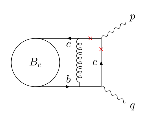
(a)

(b)

(c)

(d)

Figure 4.1: The NLO, $O(\alpha_{s})$ diagrams: (a) the box, (b),(c)- the vertices and (d)-the self-energy of $c$-quark. Crosses indicate the cuts relevant for the sum rules.

It is interesting to note that these contributions are in one-to-one correspondence with a simple picture where the wave functions of the $B_{c}$ and the $J/\psi$ states are convoluted with a hard kernel, which, to leading order, is the one-gluon exchange (cf. [6]). The two corresponding diagrams are obtained from the cut diagrams in Figs. 1(a)–1(b) if the $\bar{c}c$ vertex is replaced by the $J/\psi$ state. From this simple point of view it becomes also clear, that this new sum rule is restricted to negative and possibly also to small positive values of $q^{2}$, since at $q^{2}_{\rm max}$ the exchanged gluon becomes soft.

5 The OPE spectral density

Here we calculate separately the two contributions to the OPE spectral density, stemming from the $\bar{c}c$ cuts of the NLO box and vertex diagrams.

5.1 The $\bar{c}c$ cut of the box diagram

First, we shall obtain the full expression of the diagram in Fig. 4.1(a) in terms of a Feynman integral. Inserting in (2.1) a propagator

$$\langle 0|T\{A^{a}_{\rho}(z)A^{b}_{\omega}(y)|0\rangle=-i\delta^{ab}D_{\rho\omega}(z-y)\,=-i\delta^{ab}g_{\rho\omega}\int\frac{d^{4}k}{k^{2}}e^{ik(z-y)}$$

(in the Feynman gauge) of the gluon line between $b$ and $c$ quarks, and contracting the quark fields into free propagators

$$\langle 0|T\{Q^{i}_{\alpha}(z)\bar{Q}^{k}_{\beta}(x)|0\rangle=i\delta^{ik}S_{Q\,\alpha\beta}(z-x)\,,\leavevmode\nobreak\ \leavevmode\nobreak\ (Q=c,b)\,,$$

we obtain:

$$F_{\mu\nu}^{(box)}(p,q)=16i\pi\alpha_{s}\int d^{4}x\,e^{ipx}\int d^{4}y\int d^{4}z\langle 0|\bar{c}_{\alpha}(z)b_{\beta}(y)|\bar{B}_{c}(p+q)\rangle$$

$$\big{[}\gamma_{\rho}S_{c}(z-x)\gamma_{\mu}S_{c}(x)\Gamma_{\nu}S_{b}(-y)\gamma_{\lambda}\big{]}_{\alpha\beta}D^{\rho\lambda}(z-y)\,,$$ (5.1)

where Dirac indices are shown explicitly and the color trace is taken. The hadronic matrix element entering the above expression is transformed with a coordinate translation ,

$$\langle 0|\bar{c}_{\alpha}(z)b_{\beta}(y)|\bar{B}_{c}(p+q)\rangle=\langle 0|\bar{c}_{\alpha}(0)b_{\beta}(y-z)|\bar{B}_{c}(p+q)\rangle e^{-i(p+q)z}\,.$$ (5.2)

After that, we expand this matrix element, similarly to Eq. (3.5), in a HQET form

$$\langle 0|\bar{c}_{\alpha}(0)b_{\beta}(y-z)|\bar{B}_{c}(p+q)\rangle \simeq e^{-im_{b}v(y-z)}\sqrt{m_{B_{c}}}\langle 0|\bar{h}^{\prime}_{\alpha}(0)h_{\beta}(0)|\bar{B}_{c}(v)\rangle$$ (5.11)

$$\simeq -\frac{i}{4}e^{-im_{b}v(y-z)}f_{B_{c}}m_{B_{c}}\big{[}(1+\mathchoice{\ooalign{$\hfil\displaystyle\mkern 0.0mu/\hfil$\crcr$\displaystyle v$}}{\ooalign{$\hfil\textstyle\mkern 0.0mu/\hfil$\crcr$\textstyle v$}}{\ooalign{$\hfil\scriptstyle\mkern 0.0mu/\hfil$\crcr$\scriptstyle v$}}{\ooalign{$\hfil\scriptscriptstyle\mkern 0.0mu/\hfil$\crcr$\scriptscriptstyle v$}})\gamma_{5}\big{]}_{\beta\alpha}\,,$$

and adopt the local limit. More specifically, we neglect the contributions of operators with derivatives in the expansion around $(y\!-\!z)=0$, (see Eq. (3.7)), since they are suppressed by inverse powers of $m_{c}$. In the last equation above we also use the leading-power approximation (3.2) and (3.11). Substituting in Eq. (5.1) the hadronic matrix element (5.11) and the quark and gluon propagators in the momentum representation, we obtain the box diagram in the form of a standard Feynman integral :

$$F^{(box)}_{\mu\nu}(p,q)=-4\pi\alpha_{s}f_{B_{c}}m_{B_{c}}$$

$$\times\!\!\int\!\frac{d^{4}k}{(2\pi)^{4}}\frac{t_{\mu\nu}(p,v,k)}{\big{[}(m_{c}v-k)^{2}\!-\!m_{c}^{2}\big{]}\big{[}(m_{c}v-k-p)^{2}\!-\!m_{c}^{2}\big{]}\big{[}(m_{b}v+k)^{2}\!-\!m_{b}^{2}\big{]}k^{2}}\,,$$ (5.12)

where the dependence on $q$ is implicit via $v=(p+q)/M$, and the trace is reduced to

$$t^{(box)}_{\mu\nu}(p,v,k)=2\mbox{Tr}[(-m_{c}\not{v}+\not{k}+m_{c})\gamma_{\mu}(-m_{c}\not{v}+\not{k}+\not{p}+m_{c})\Gamma_{\nu}(m_{b}\not{v}+\not{k}+m_{b})(2-\not{v})\gamma_{5}]\,.$$ (5.13)

We further decompose Eq. (5.12) to account for the vector and axial components of the weak current:

$$F^{(box)}_{\mu\nu}(p,v,k)=F^{V(box)}_{\mu\nu}(p,v,k)+F^{A(box)}_{\mu\nu}(p,v,k)\,,$$

putting respectively, $\Gamma_{\nu}\to\gamma_{\nu}$ and $\Gamma_{\nu}\to-\gamma_{\nu}\gamma_{5}$. The trace (5.13) splits into the two parts $t^{V(box)}_{\mu\nu}$ and $t^{A(box)}_{\mu\nu}$. In the case of the vector current, we find:

$$t^{V(box)}_{\mu\nu}(p,v,k)=-8\,i\epsilon_{\mu\nu\alpha\beta}\Big{(}k^{\alpha}p^{\beta}\big{[}m_{b}\!-\!m_{c}\!-\!2(k\cdot v)\big{]}$$

$$+k^{\alpha}v^{\beta}\big{[}2m_{c}(k\cdot v)-k^{2}\big{]}-v^{\alpha}p^{\beta}\big{[}2m_{b}m_{c}-k^{2}\big{]}\Big{)}\,.$$ (5.14)

A bulky expression for the trace with the axial current is presented in Appendix C, see Eq. (• ‣ C).

The vector and axial parts of Eq. (5.12) with the traces given in Eq. (5.14) and Eq. (• ‣ C) contain the following scalar, vector and tensor integrals differing by the number of four-momenta $k$ in the numerator:

$$I^{b}_{\{1,\,\alpha,\,\alpha\beta,\,\alpha\beta(v)\}}(p^{2},q^{2})\equiv\!-i\!\!\int\!\frac{d^{4}k}{(2\pi)^{4}}\!\!\frac{\{1,\,k_{\alpha},k_{\alpha}k_{\beta},\,k_{\alpha}k_{\beta}(k\cdot v)\}}{k^{2}\big{[}(m_{b}v\!+\!k)^{2}\!-\!m_{b}^{2}\big{]}\big{[}(m_{c}v\!-\!k\!-\!p)^{2}\!-\!m_{c}^{2}\big{]}\big{[}(m_{c}v\!-\!k)^{2}\!-\!m_{c}^{2}\big{]}}$$ (5.15)

where the index $b$ indicates the box diagram . Furthermore, the terms in Eq. (5.12) with $k^{2}$ in the numerator are reduced to the three simpler integrals which we denote as $J_{1}^{b},J_{\alpha}^{b},J_{\alpha\beta}^{b}$. They are obtained, respectively, from $I_{1}^{b},I_{\alpha}^{b},I_{\alpha\beta}^{b}$, removing $k^{2}$ in the denominator. We are interested only in the imaginary part of the integrals listed above. In Appendix A, a detailed calculation for the scalar integral $I_{1}^{b}$ is presented, where using the Cutkosky rule, we obtain $\mbox{Im}I_{1}^{b}$. In Appendix B, decompositions of the imaginary parts of the vector and tensor integrals are presented. The coefficients in these decompositions are obtained by a reduction to scalar integrals. We rewrite the vector-current part of the box diagram contribution in terms of master integrals defined in Eq. (5.15):

$$F^{V(box)}_{\mu\nu}(p,q)=32i\pi\alpha_{s}f_{B_{c}}m_{B_{c}}\epsilon_{\mu\nu\alpha\beta}\bigg{\{}I^{b\,\alpha}p^{\beta}(m_{b}-m_{c})-2I^{b\,\alpha\lambda}v_{\lambda}p^{\beta}+2m_{c}I^{b\,\alpha\lambda}v_{\lambda}v^{\beta}$$

$$-J^{b\,\alpha}v^{\beta}-v^{\alpha}p^{\beta}(2m_{b}m_{c}I_{1}^{b}-J_{1}^{b})\bigg{\}}\,.$$ (5.16)

The corresponding expression for the axial-current part is given in Appendix C, in Eq. (C.3)

To obtain the imaginary part of Eq. (5.16), we use the decompositions of the imaginary parts of vector ans tensor integrals in terms of invariant coefficients presented in Appendix B. Assuming the invariant amplitude for the vector current is defined as in Eq. (2.1), where we replace $\epsilon_{\mu\nu\alpha\beta}\,q^{\alpha}p^{\beta}=-m_{B_{c}}\epsilon_{\mu\nu\alpha\beta}\,p^{\alpha}v^{\beta}$, we finally obtain:

$$\mbox{Im}F^{V(box)}(p^{2},q^{2})=-32i\pi\alpha_{s}f_{B_{c}}\big{[}2m_{b}m_{c}\mbox{Im}I_{1}^{b}-(m_{b}-m_{c})A^{b}-B_{J}^{b}$$

$$+C^{b}+2m_{c}D^{b}+(2m_{c}(p\cdot v)-p^{2})F^{b}-2G^{b}\big{]}\,,$$ (5.17)

where the expressions for $\mbox{Im}I_{1}^{b}$ and for the coefficients $A^{b}$, $B_{J}^{b}$ , $C^{b}$, $D^{b}$, $F^{b}$, $G^{b}$ are given in Appendix A and Appendix B, respectively. For the axial-current part, the resulting expression for $\mbox{Im}F^{A(box)}_{\mu\nu}$ is given in Appendix C, in Eq. (C.5).

5.2 The $\bar{c}c$-cut of the vertex diagram

The amplitude corresponding to the vertex diagram in Fig. 4.1(b) is derived analogously as for the box diagram, leading to the complete Feynman integral:

$$F^{(vert)}_{\mu\nu}(p,q)=\frac{4\pi\alpha_{s}f_{B_{c}}m_{B_{c}}}{(m_{b}v-q)^{2}-m_{c}^{2}}\!\!\int\!\frac{d^{4}k}{(2\pi)^{4}}\frac{t^{vert}_{\mu\nu}(p,v,k)}{\big{[}(k-m_{c}v)^{2}\!-\!m_{c}^{2}\big{]}\big{[}(k+p-m_{c}v)^{2}\!-\!m_{c}^{2}\big{]}k^{2}}\,,$$ (5.18)

with the trace

$$t^{(vert)}_{\mu\nu}(p,v,k)=\mbox{Tr}\big{(}\gamma^{\rho}(\not{k}-m_{c}\not{v}+m_{c})\gamma_{\mu}(\not{k}+\not{p}-m_{c}\not{v}+m_{c})\gamma_{\rho}(m_{b}\not{v}-\not{q}+m_{c})\Gamma_{\nu}(1+\not{v})\gamma_{5}\big{)}\,.$$

We split Eq. (5.18) into the vector-current and axial-current parts:

$$F^{(vert)}_{\mu\nu}(p,v)=F^{V(vert)}_{\mu\nu}(p,v)+F^{A(vert)}_{\mu\nu}(p,v)\,,$$

with the corresponding traces:

$$t^{V(vert)}_{\mu\nu}(p,v,k)=8\,i\epsilon_{\mu\nu\alpha\beta}\!\Big{[}-2k^{\alpha}p^{\beta}m_{c}+k^{\alpha}v^{\beta}p^{2}$$

$$+v^{\alpha}p^{\beta}\big{[}2m_{c}^{2}-2(v\cdot p)m_{c}-2(k\cdot v)m_{c}+k^{2}+2(k\cdot p)\big{]}\Big{]}-16i\epsilon_{\rho\alpha\beta\nu}k^{\rho}v^{\alpha}p^{\beta}k_{\mu}$$

$$+16i\epsilon_{\rho\alpha\beta\mu}k^{\rho}v^{\alpha}p^{\beta}v_{\nu}m_{c}+16i\epsilon_{\rho\alpha\beta\nu}k^{\rho}v^{\alpha}p^{\beta}v_{\mu}m_{c}-16i\epsilon_{\rho\alpha\beta\nu}k^{\rho}v^{\alpha}p^{\beta}p_{\mu}\,,$$ (5.19)

and $t^{A(vert)}_{\mu\nu}(p,v,k)$ presented in the Appendix C, in Eq. (C.2).

Note that the $c$-quark propagator multiplying the integral in Eq. (5.18) yields a simple pole located at the same $p^{2}$ value (4.2) as in the LO diagram. Since we are only interested in the contributions to the imaginary part of $F_{\mu\nu}^{(vert)}$ within the duality interval (4.1) and at $q^{2}\lesssim 0$, this pole located far above that interval yields a real-valued coefficient. Hence, to compute the imaginary part of Eq. (5.18), we only have to apply Cutkosky rules to the two $c$-quark propagators under the integral.

The full calculation of the integral in Eq. (5.18) requires five integrals, $I^{v}_{1}$, $I_{\alpha}^{v}$, I${}_{\alpha\beta}^{v}$, $J_{1}^{v}$, and $J^{v}_{\alpha}$, where we use the same nomenclature as for the box diagram with the index $v$ distinguishing the vertex diagram. The vector-current part in terms of this notation reads:

$$F^{V(vert)}_{\mu\nu}(p,q)=\frac{32i\pi\alpha_{s}f_{B_{c}}m_{B_{c}}}{(m_{b}v-q)^{2}-m_{c}^{2}}\bigg{\{}\epsilon_{\mu\nu\alpha\beta}\bigg{[} -2m_{c}I^{v\,\alpha}p^{\beta}+p^{2}I^{v\,\alpha}v^{\beta}+v^{\alpha}p^{\beta}\big{(}2m_{c}(m_{c}-vp)I_{1}^{v}$$ (5.20)

$$-2m_{c}v^{\lambda}I_{\lambda}^{v}+J_{1}^{v}+2p^{\lambda}I_{\lambda}^{v}\big{)}\bigg{]}-2\epsilon_{\rho\alpha\beta\nu}v^{\alpha}p^{\beta}I_{\rho\mu}^{v}\bigg{\}}$$

and the expression for the axial-current part is given in Appendix C, in Eq. (C.4).

Substituting the imaginary parts of the integrals from Appendix B, we obtain from Eq. (5.20):

$$\mbox{Im}F^{V(vert)}(p^{2},q^{2})=\frac{32i\pi\alpha_{s}f_{B_{c}}}{2m_{c}(p\cdot v)\!-\!p^{2}}\Bigg{[}2m_{c}\big{(}(p\!\cdot\!v)\!-\!m_{c}\big{)}\mbox{Im}I_{1}^{v}$$

$$+2(m_{c}\!-\!(p\!\cdot\!v))A^{v}-p^{2}B^{v}+2G^{v}\Bigg{]}\,,$$ (5.21)

where $(p\!\cdot\!v)=p_{0}$ as a function of $p^{2},q^{2}$ is taken from Eq. (3.15). The corresponding expression for the imaginary part of the axial-current contribution is in Appendix C, in Eq. (C.6). The imaginary part of the scalar integral $\mbox{Im}I_{1}^{v}$ is derived in Appendix A and expressions for all other coefficients in Eq. (5.21) and in Eq. (C.6) are obtained in Appendix B.

Adding together the box and vertex diagram contributions, given by Eq. (5.17) and Eq. (5.21), respectively, we finally obtain the OPE spectral density

$$\mbox{Im}F^{V(OPE)}(s,q^{2})=\mbox{Im}F^{V(box)}(s,q^{2})+\mbox{Im}F^{V(vert)}(s,q^{2})\,,$$ (5.22)

entering the sum rule (2.10) for the $B_{c}\to J/\psi$ vector form factor in the adopted approximation.

For the axial-current form factors the analogous results for the OPE spectral densities entering the sum rules (2.11),(2.12) and (2.13) are obtained from:

$$\mbox{Im}F^{A(OPE)}_{(i)}(s,q^{2})=\mbox{Im}F_{(i)}^{A(box)}(s,q^{2})+\mbox{Im}F_{(i)}^{A(vert)}(s,q^{2})\,,\leavevmode\nobreak\ \leavevmode\nobreak\ (i)=(g),(qp),(qq)\,,$$ (5.23)

respectively, where all separate contributions are presented in Appendix C, in Eqs (C.9) - (C.14).

6 Numerical analysis

Here we obtain numerical results for the $B_{c}\to J/\psi$ form factors. We use the Borel sum rules in Eqs. (2.10)–(2.13). Their power moments such as Eq. (2.14) serve as a comparison.

The inputs used in our numerical analysis are collected in Table 6.1.

Parameter	Value
$\overline{m}_{b}(\overline{m}_{b})$	$4.18^{+0.03}_{-0.02}\,\mathrm{GeV}$[22]
$\overline{m}_{c}(\overline{m}_{c})$	$1.27\pm 0.02\,\mathrm{GeV}$ [22]
$\alpha_{s}(m_{Z})$	$0.1179\pm 0.0009$ [22]
$\mu$	$3.0\pm 0.5$ GeV
$\alpha_{s}(\mu)$	$0.2530\pm 0.0187$
$m_{B_{c}}$	6.27448 $\pm$ 0.00032  GeV [22]
$f_{B_{c}}$	$0.434\pm 0.015\,\mathrm{GeV}$ [23]
$f_{J/\psi}$	$0.416\pm 0.06\,\mathrm{GeV}$ [22]
$m_{J/\psi}$	$3.096900\pm 0.000006\,\mathrm{GeV}$ [22]
${\cal M}^{2}$	3.0 $\pm$ 2.0 GeV2

Table 6.1: Input parameters used in the sum rules (2.10)-(2.13).

For the $b$ and $c$ quark masses, there is a certain freedom in choosing their renormalization scheme. In the correlation function (2.1), both heavy quarks participate in two different ways: firstly, they form the initial $B_{c}$ meson in a static approximation, and, secondly, they perturbatively propagate between the vertices and annihilate into external currents. To account for both long-distance and short-distance dynamics of $b$ and $c$ quarks, we choose the pole scheme for their masses. This has certain advantages with respect to the $\overline{\mathrm{MS}}$ scheme which is a standard choice for conventional QCD sum rules. Indeed, the use of the $\overline{\mathrm{MS}}$ masses $\overline{m}_{b}$ and $\overline{m}_{c}$ will bring the problem of fixing a normalization scale. Moreover, the difference between the mass of $B_{c}$ and the sum $\overline{m}_{b}+\overline{m}_{c}$ becomes rather large to be treated as a soft scale. We then employ the relation between the pole mass and $\overline{\mathrm{MS}}$ mass at $\mathcal{O}(\alpha_{s})$ accuracy,

$$m_{Q}^{pole}=\overline{m}_{Q}(\overline{m}_{Q})\left(1+\frac{4\alpha_{s}(\overline{m}_{Q})}{3\pi}\right)\,,\leavevmode\nobreak\ \leavevmode\nobreak\ \leavevmode\nobreak\ Q=b,c.$$ (6.1)

Using for the $\overline{\mathrm{MS}}$ masses their world averages from [22] yields:

$$m_{b}^{pole}=4.58\pm 0.03\leavevmode\nobreak\ \mbox{GeV},\leavevmode\nobreak\ \leavevmode\nobreak\ \leavevmode\nobreak\ \leavevmode\nobreak\ m_{c}^{pole}=1.48\pm 0.02\leavevmode\nobreak\ \mbox{GeV}\,,$$ (6.2)

where we just take into account the parametric errors from the variation of the $\overline{\mathrm{MS}}$ masses and $\alpha_{s}$. Since we work in the leading power approximation, the $\mathcal{O}(\Lambda_{QCD}/m_{Q})$ uncertainty of the pole mass related to long-distance effects is neglected.

To choose an optimal renormalization scale for $\alpha_{s}$, ideally, one should calculate the $\mathcal{O}(\alpha_{s}^{2})$ corrections, which are far beyond our scope and represent a technically challenging task for the future. We find useful information concerning the scale choice in Ref. [6], where gluon radiative corrections to the one-gluon exchange were calculated in the framework of a non-relativistic bound-state picture of the $B_{c}\to$ charmonium transition at large recoil. There it was shown that large logarithms are absent if the scale is in the ballpark of $\mu\sim\sqrt{m_{b}m_{c}}$, which for the masses in Eq. (6.2) corresponds to $\mu=2.6\pm 0.03$ GeV. The broader interval of $\mu$ that we adopt is consistent with this prescription.

The main advantage of our sum rules is that the OPE contains a single non-perturbative parameter – the $B_{c}$-meson decay constant. The latter can be directly measured in the leptonic decay $B_{c}\to\mu\nu$, which, however, has not been detected yet. We use the $f_{B_{c}}$ value obtained from lattice QCD in [23]. In the past, two-point QCD sum rules were also used to calculate $f_{B_{c}}$ (see, e.g., [9] - [11]). The predicted values are, within uncertainties, in agreement with the lattice QCD results. The remaining hadronic input parameters include the accurately measured masses of the $B_{c}$ and the $J/\psi$, and the decay constant of the $J/\psi$. The latter is calculated directly from the measured leptonic width of the $J/\psi$.

Finally, we comment on the choice of the Borel mass interval in Table 6.1. In the conventional QCD sum rules based on the vacuum correlation functions and condensate expansion, two conditions have to be satisfied within this interval: i) small power corrections, and ii) moderate contributions of excited and continuum states estimated using duality. An indication that both conditions are fulfilled is the stability of the sum rule prediction with respect to the variation of $\mathcal{M}^{2}$. In our setup, the conditions i) and ii) cannot be readily imposed, since the power corrections are neglected and the OPE spectral density is calculated only in the interval near $4m_{c}^{2}$. Instead, we use information from the well-known 2-point QCD sum rules for vector charmonium, which use the same interpolating current $\bar{c}\gamma_{\mu}c$ as the one in our correlation function. Traditionally, starting from the original work [15], the charmonium sum rules were analysed using power moments. The latter were obtained, similarly to Eq. (2.14), by a multiple differentiation over the external momentum square $q^{2}$ and at a certain spacelike point $q^{2}=-P^{2}$. There were, however, also several analyses of the same sum rules using the Borel version, see e.g. Refs. [24, 25], using the interval $1.0<\mathcal{M}^{2}<5.0$ GeV², which we also adopt. To validate this choice, we recalculated the power moments of two-point sum rules at a typical value $P^{2}=4m_{c}^{2}$ and at $n=2,3,4$. We took into account the $\mathcal{O}(\alpha_{s})$ terms in the perturbative part and the gluon condensate contribution, using the analytical expressions from [15]. We found that both the mass and decay constant of the $J/\psi$ are reproduced within $\leq 5\%$ accuracy. The moments with $n>4$ are not reliable because the power correction due to the gluon condensate becomes too large, whereas $n=1$ yields too large contribution of charmonia above the $J/\psi$ (c.f. the above criteria i) and ii), respectively). According to the approximate connection between the Borel parameter and moments, the optimal set of power moments corresponds to the interval 2.2 GeV² $<{\cal M}^{2}=P^{2}/n<4.4$ GeV², which is within our adopted interval in Table 6.1.

The remaining element of the numerical analysis is the value of the effective threshold in the Borel sum rules. We determine it for the vector-current case, Eq. (2.10) and use it for the other sum rules. To this end, we apply a standard tool, namely taking the derivative of the Borel sum rule over $-1/{\cal M}^{2}$ and dividing the result by the initial sum rule. The ratio

$$\frac{\int\limits_{4m_{c}^{2}}^{s_{0}}\!ds\,se^{-s/{\cal M}^{2}}\mbox{Im}F^{V(OPE)}(s,q^{2})}{\int\limits_{4m_{c}^{2}}^{s_{0}}\!ds\,e^{-s/{\cal M}^{2}}\mbox{Im}F^{V(OPE)}(s,q^{2})}=m_{J/\psi}^{2}\,$$ (6.3)

is independent of the form factor and allows us to determine $s_{0}$ by fitting l.h.s. to the $J/\psi$ mass. We find that in the whole region $1.0\leavevmode\nobreak\ \mbox{GeV}^{2}<\mathcal{M}^{2}<5.0\leavevmode\nobreak\ \mbox{GeV}^{2}$ and at $-20.0\leavevmode\nobreak\ \mbox{GeV}^{2}<q^{2}<0$ the value $s_{0}=10.2$ GeV² being substituted as a threshold, yields the l.h.s of (6.3) equal the squared mass of the $J/\psi$ within $\leq 2\%$. Note that this value of $s_{0}$ is substantially lower than a typical duality threshold for the two-point sum rules which is close to the mass of $\psi(2S)$. This is not surprising, taking into account that here we have a completely different behaviour of the OPE spectral density above the threshold $4m_{c}^{2}$.

With the chosen input, we obtain from the sum rules in Eqs. (2.10)–(2.13) numerical values for all $B_{c}\to J/\psi$ form factors in the range of momentum transfer $-20\leavevmode\nobreak\ \mbox{GeV}^{2}<q^{2}<0$. Changing the Borel parameter within the interval in Table 6.1, we find that at $q^{2}=0$ the resulting variations of all form factors at $\mathcal{M}^{2}=5.0$ GeV² ($\mathcal{M}^{2}=1.0$ GeV²) do not exceed $-2\%$ ($+6\%$ ) of their values at $\mathcal{M}^{2}=3.0$ GeV². Moreover, at negative $q^{2}<-10$ GeV² the form factors are practically constant with respect to the Borel mass variation. Thus, we reveal reasonable stability of the sum rule results, which is an important indication that the neglected power corrections are not large.

Form factor	Method	$q^{2}=-20\,\mathrm{GeV}^{2}$	$q^{2}=-10\,\mathrm{GeV}^{2}$	$q^{2}=0$
$V$	(1)	0.045	0.116	0.740
	(2)	0.046	0.117	0.753
$A_{1}$	(1)	0.043	0.093	0.472
	(2)	0.043	0.094	0.480
$A_{2}$	(1)	0.034	0.084	0.487
	(2)	0.034	0.084	0.495
$A_{0}$	(1)	0.030	0.073	0.464
	(2)	0.030	0.074	0.473

Table 6.2: Numerical results for the $B_{c}\to J/\psi$ form factors obtained from: (1) the Borel sum rules at ${\cal M}^{2}=3.0\leavevmode\nobreak\ \mbox{GeV}^{2}$ and (2) the power moment sum rules with $n=3$ at $P^{2}=4m_{c}^{2}$. All other input parameters are taken at central values.

Another test of our method is a comparison of the Borel sum rules with the power moments. In Table 6.2 we present the form factors, obtained from these two versions of sum rules, setting the input parameters at their central values. Taking $P^{2}/n$ maximally close to ${\cal M}^{2}$, we observe a good agreement, especially at $q^{2}<0$.

Our main results on the form factors are presented in Table 6.3. To obtain the uncertainties of the form factors, we varied all the parameters in Table 6.1, apart from $\mathcal{M}^{2}$ to a multivariate normal distribution, that is, uniformly in the interval $1.0\,\mathrm{GeV}^{2}<\mathcal{M}^{2}<5.0\,\mathrm{GeV}^{2}$. As a result of this procedure, we find that the predictions for the form factors do not follow a normal distribution, hence the asymmetric uncertainties in Table 6.3. The largest uncertainty, in the ballpark of $\pm 30\%$, is caused by the variation of the $c$-quark mass, whereas the uncertainty related to the $b$-quark mass turns out to be at a percent level. This specific property of our sum rules is caused by the fact that the lower threshold of the integrals depends only on $m_{c}$ . The second and third in size effects influencing uncertainties are, respectively, the errors of $\alpha_{s}$ and $f_{B_{c}}$.

In Table 6.3, we also compare our predictions at $q^{2}=0$ to the lattice QCD results [4], finding a reasonable agreement. Concerning the $q^{2}$ dependence, we find that the form factors based on the new sum rules are highly correlated, preventing from a reliable extrapolation to the semileptonic region $0<q^{2}<(m_{B_{c}}-m_{J/\psi})^{2}$.

For comparison, in Fig. 6.1, we plot the $q^{2}$ dependence of the $B\to J/\psi$ form factors obtained from the sum rules and in the lattice QCD [4]. The two approaches are valid in the two complementary regions of $q^{2}$. In addition, we used the $z$-expansion obtained from the lattice QCD analysis in [4] and analytically continued it towards negative $q^{2}$. Within uncertainties, only a marginal agreement between the slopes is observed.

Form factor	$q^{2}=-20\,\mathrm{GeV}^{2}$	$q^{2}=-10\,\mathrm{GeV}^{2}$	$q^{2}=0$	HPQCD at $q^{2}=0$ [4]
$V$	$0.044^{+0.016}_{-0.013}$	$0.112^{+0.043}_{-0.035}$	$0.705^{+0.364}_{-0.253}$	$0.725\pm 0.055$
$A_{1}$	$0.042^{+0.015}_{-0.012}$	$0.090^{+0.034}_{-0.027}$	$0.451^{+0.222}_{-0.158}$	$0.457\pm 0.027$
$A_{0}$	$0.028^{+0.010}_{-0.008}$	$0.071^{+0.026}_{-0.021}$	$0.443^{+0.219}_{-0.156}$	$0.4770\pm 0.026$
$A_{2}$	$0.033^{+0.012}_{-0.010}$	$0.081^{+0.031}_{-0.025}$	$0.466^{+0.228}_{-0.162}$	$0.418\pm 0.086$
$A_{12}$	$0.009^{+0.003}_{-0.002}$	$0.017^{+0.006}_{-0.005}$	$0.085^{+0.042}_{-0.030}$	$0.091\pm 0.008$

Table 6.3: Numerical results for the $B_{c}\to J/\psi$ form factors. The central values (asymmetric uncertainties) correspond to the medians of the distributions (the $68\%$ confidence intervals).

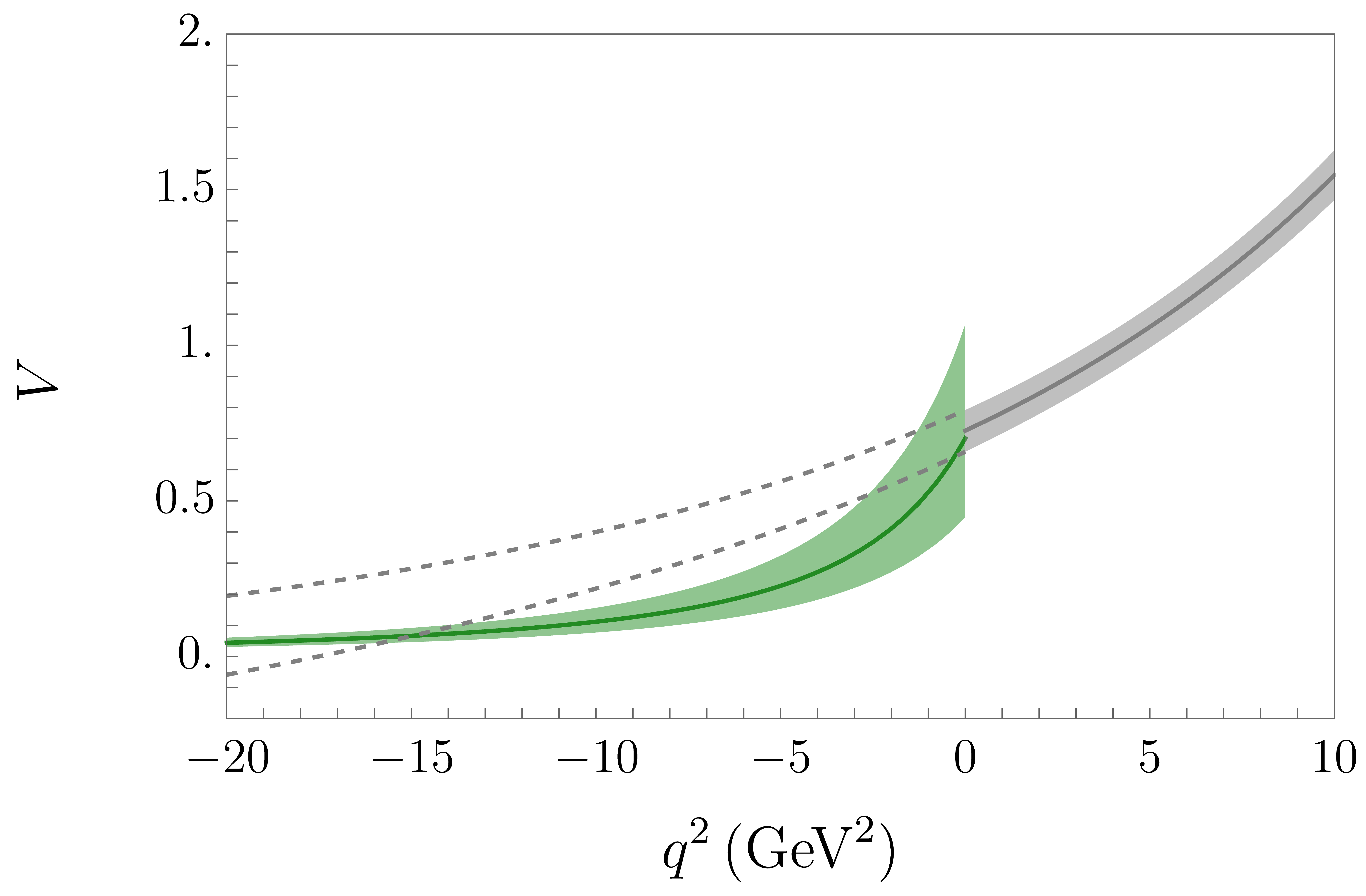
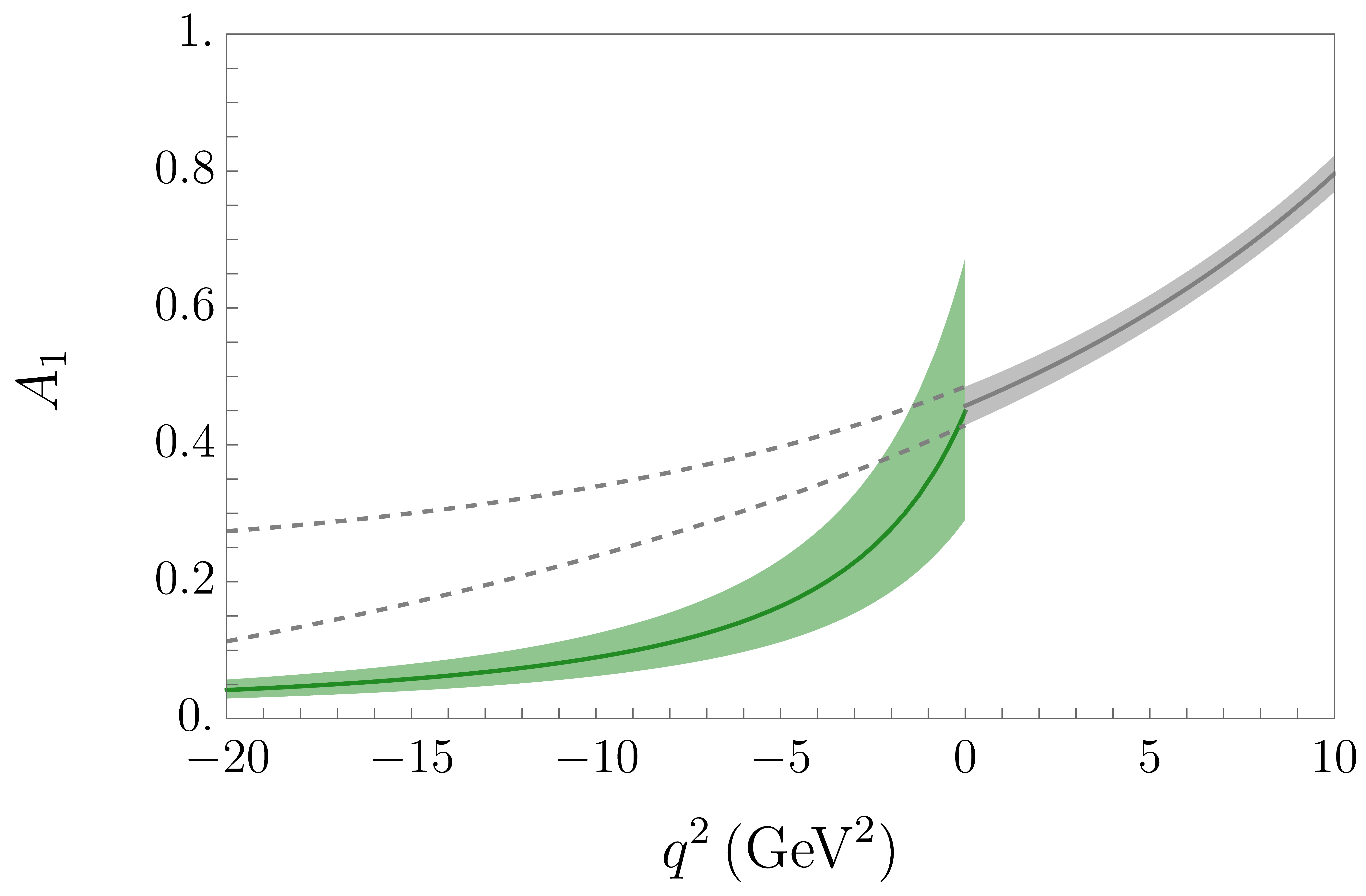
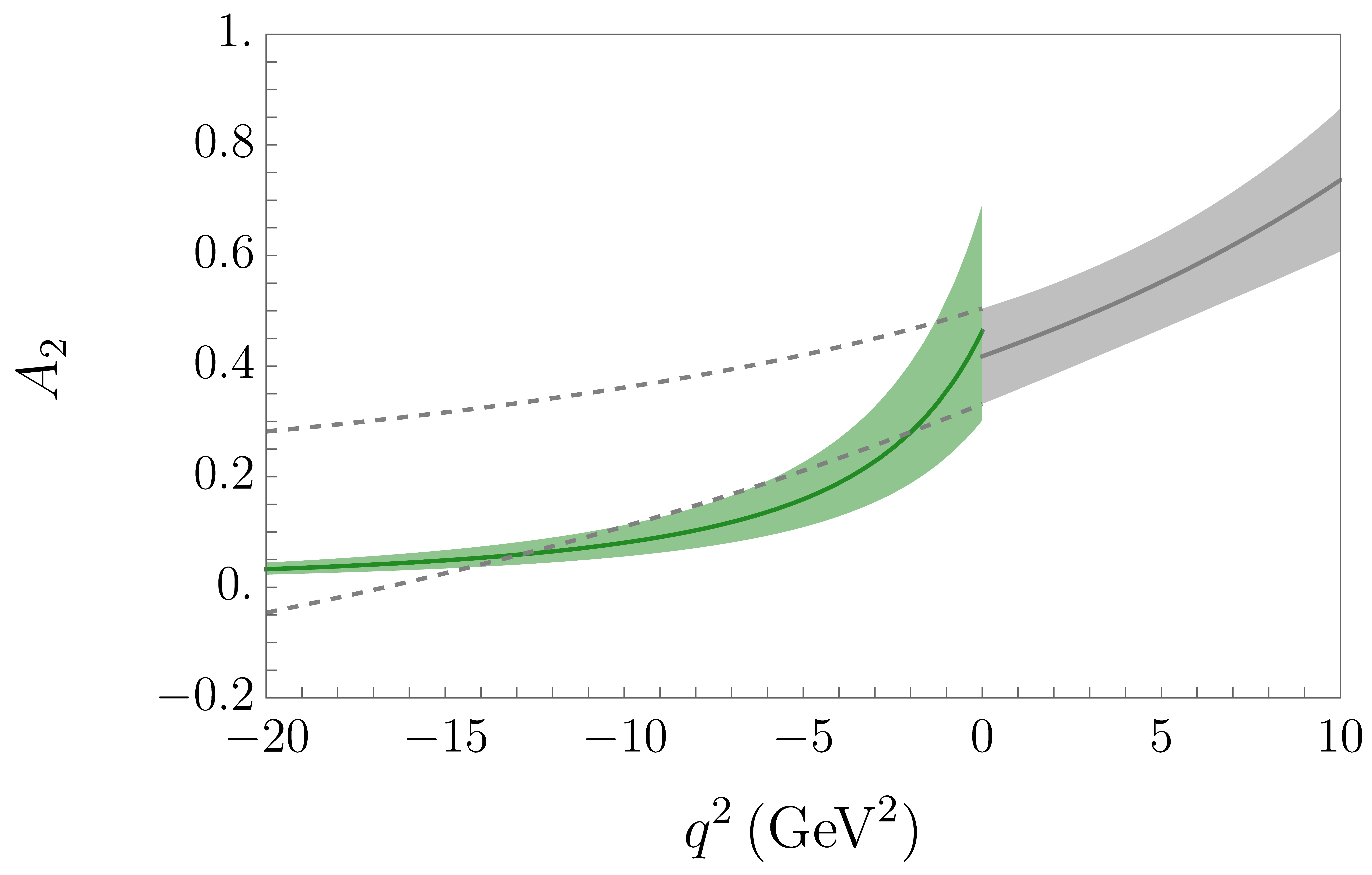
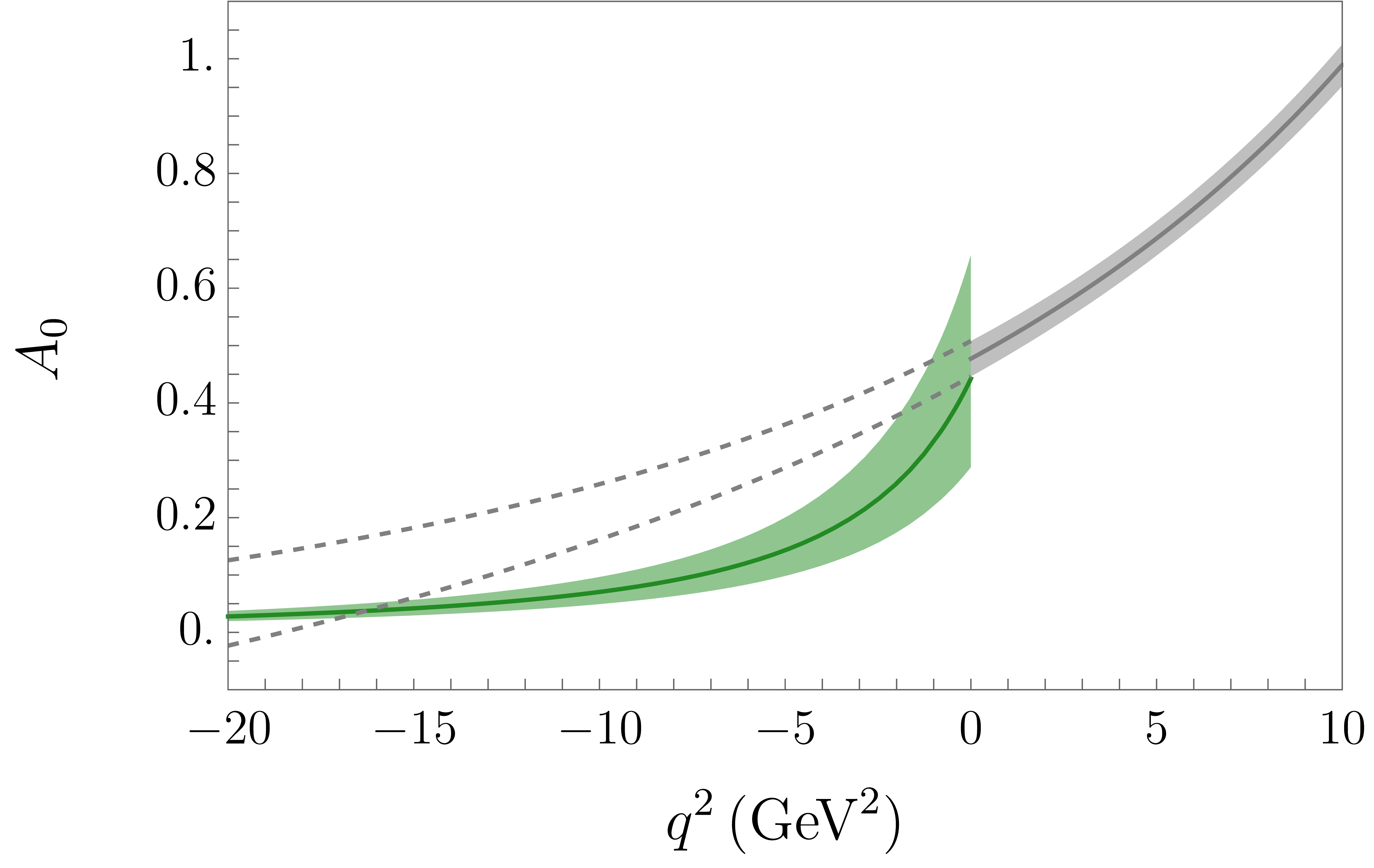
Figure 6.1: Results for the vector and axial-vector $B_{c}\to J/\psi$ form factors. The green band represents the 68% C.L. region for the sum rule results at $q^{2}<0$. The gray bands are the 68% C.L. region for the lattice QCD predictions [4] at $q^{2}>0$. The solid green and gray lines in the center show the median of the sum rules and lattice QCD results distribution, respectively.

7 Conclusion

In this paper, we derive new QCD sum rules for the $B_{c}\to J/\psi$ form factors. We use a $B_{c}$-to-vacuum correlation function of the weak $b\to c$ and interpolating $\bar{c}\gamma_{\mu}c$ currents, retaining finite $b$ and $c$ quark masses. The $B_{c}\to J/\psi$ form factors are then related to the correlation function via the hadronic dispersion relation in the momentum squared of the interpolating current.

We find and use two generally unexpected properties of the underlying correlation function, valid in the heavy-quark limit, $m_{b},m_{c}\gg\Lambda_{QCD}$. First, due to the presence of a heavy spectator $\bar{c}$-quark in $B_{c}$, a local OPE is valid in the $q^{2}\lesssim 0$ region of a large recoil to the final state. The non-perturbative input, at the leading power in $1/m_{b,c}$ is reduced to a single parameter – the decay constant of $B_{c}$ meson. Second, in the same region $q^{2}\lesssim 0$, the OPE spectral density in the duality interval for $J/\psi$ starts at $\mathcal{O}(\alpha_{s})$. This is in accordance with an expected dominance of the hard-gluon exchange in the $B_{c}\to J/\psi$ transition at large recoil.

Derivation of the sum rules and calculation of the OPE diagrams performed in this paper is just a first step in the exploration of the new sum rules. We foresee other important applications with various final $\bar{c}c$ states in $B_{c}$ decays.

The accuracy of the new sum rules can also be improved in the future. The unaccounted next-to-leading power corrections proportional to the inverse $b$ and $c$ quark masses should be identified and estimated. Their systematic analysis will demand technically more involved but straightforward computational procedures, leading to a couple of new input parameters. Improving also the perturbative part of the sum rules, one has to calculate the two-gluon exchanges at $O(\alpha_{s}^{2})$. Here the Coulomb gluons have to be factorized from the hard gluons. At this level of accuracy, the NRQCD description of the initial $B_{c}$ state can be used and combined with the new sum rules.

Altogether, we believe that our approach is more adequate for describing the $B_{c}\to$ charmonium transitions than the traditional framework of three-point QCD sum rules used in the past, mainly because the latter sum rules still miss important but technically inaccessible hard-gluon effects.

Finally, we perform a numerical analysis of the leading order term. We find that near $q^{2}=0$, the form factors calculated with our method agree with the most advanced lattice QCD predictions. Still, strong correlations between the sum rule numerical results at different $q^{2}<0$ points do not allow us to obtain a reliable extrapolation to the semileptonic region, with the help of e.g., a $z$ expansion.

Concluding, the new QCD sum rules have the potential to provide the $B_{c}\to$ charmonium form factors at large recoil and can complement the lattice QCD results in the flavour-oriented applications of these form factors.

Appendix A Imaginary parts of the scalar integrals

Here we compute the imaginary part of the scalar master integrals corresponding to the $\bar{c}c$ cut in the diagrams in Figs. 1(a)–1(b).

A.1 Box diagram

We start from the expression in Eq. (5.15) for $I_{1}^{b}$ and apply Cutkosky rules to both $c$-quark propagators :

$$2\mbox{Im}\,I_{1}^{b} = \int\frac{d^{4}k}{(2\pi)^{4}}\frac{1}{k^{2}[(m_{b}v+k)^{2}-m_{b}^{2}]}$$ (A.1)

$$\times (2\pi)\delta_{+}((m_{c}v-k)^{2}-m_{c}^{2})\,(2\pi)\delta_{-}((m_{c}v-k-p)^{2}-m_{c}^{2})\,,$$

where for a generic on-shell momentum $P$, $P^{2}=m^{2}$, we denote

$$\delta_{\pm}(P^{2}-m^{2})=\theta(\pm P_{0})\delta(P^{2}-m^{2})\,.$$

Note that for the kinematic branch we are interested in, we have to pick the antiparticle part of the cut charm propagator, hence the $\delta_{-}$ -function.

The on-shell $\delta$-functions imply

$$(m_{c}v-k)^{2}-m_{c}^{2}=k^{2}-2m_{c}(k\cdot v)=0\,,$$ (A.2)

$$(m_{c}v-k-p)^{2}-m_{c}^{2}=p^{2}-2m_{c}(p\cdot v)+2(k\cdot p)=0\,,$$ (A.3)

and we can write:

$$2\mbox{Im}I^{b}_{1}=\int\frac{d^{4}k}{(2\pi)^{2}}\frac{1}{2m_{c}(k\cdot v)}\frac{1}{2M(k\cdot v)}\delta(k^{2}-2m_{c}(k\cdot v))\theta(m_{c}-(k\cdot v))$$

$$\qquad\times\delta(p^{2}-2m_{c}(p\cdot v)+2(k\cdot p))\theta((p\cdot v)+(k\cdot v)-m_{c})\,,$$ (A.4)

where $M=m_{b}+m_{c}$.

In the reference frame (3.14) of our choice

$$k\cdot v=k_{0}\,,\quad p\cdot v=p_{0}\,,\quad k^{2}=k_{0}^{2}-\kappa^{2}\,,\quad p^{2}=p_{0}^{2}-\vec{p}^{\,2}\,,$$ (A.5)

where $\kappa\equiv|\vec{k}|$. Hence, (A.2) implies, together with $\theta(m_{c}-(k\cdot v))=\theta(m_{c}-k_{0})$,

$$k_{0}=m_{c}-\sqrt{\kappa^{2}+m_{c}^{2}}\equiv m_{c}-E_{\kappa}\leq 0\,.$$ (A.6)

We rewrite the $\delta$-function corresponding to Eq. (A.2) as a function of $k_{0}$, finding:

$$\delta\big{(}k^{2}-2m_{c}(k\cdot v)\big{)}\theta\big{(}m_{c}-(k\cdot v)\big{)}=\delta(k_{0}-m_{c}+E_{\kappa})\frac{1}{2E_{\kappa}}\,.$$ (A.7)

Performing the $k_{0}$ integration in (A.4), we get

$$2\mbox{Im}I_{1}^{b}=\frac{1}{8m_{c}M}\int\frac{d^{3}k}{(2\pi)^{2}}\frac{1}{(m_{c}-E_{\kappa})^{2}E_{\kappa}}\delta\big{(}p^{2}-2m_{c}p_{0}+2(k\cdot p)\big{)}\theta\big{(}p_{0}-E_{\kappa}\big{)}\,.$$ (A.8)

The remaining scalar product evaluated in the frame (3.14) is:

$$k\cdot p=p_{0}(m_{c}-E_{\kappa})-\kappa|\vec{p}\,|\cos\Theta\,,$$ (A.9)

where the angle $\Theta$ is between $\vec{p}$ and $\vec{k}$. The 3-momentum integration can be written as

$$\frac{d^{3}k}{(2\pi)^{2}}=\frac{1}{2\pi}\kappa^{2}\,d\kappa\,d(\cos\Theta)=\frac{1}{2\pi}\kappa^{2}\,d\kappa\,du\,\theta(1-u)\theta(1+u)$$ (A.10)

with $u=\cos\Theta$. The remaining $\delta$-function in Eq. (A.8) fixes the value of the variable $u$:

$$p^{2}-2m_{c}p_{0}+2(k\cdot p)=p_{0}^{2}-|\vec{p}\,|^{2}-2m_{c}p_{0}+2p_{0}(m_{c}-E_{\kappa})-2\kappa|\vec{p}\,|u=0\,,$$ (A.11)

so that

$$u_{*}=\frac{1}{2\kappa|\vec{p}\,|}(p_{0}^{2}-|\vec{p}\,|^{2}-2p_{0}E_{\kappa})\,,$$ (A.12)

allowing us to transform the integral (A.8) into

$$2\mbox{Im}I_{1}^{b}=\frac{1}{32\pi|\vec{p}\,|m_{c}M}\int\frac{\kappa\,d\kappa}{(m_{c}-E_{\kappa})^{2}E_{\kappa}}\theta(p_{0}-E_{\kappa})\theta(\kappa)\theta(1-u_{*})\theta(1+u_{*})$$

$$=\frac{1}{32\pi|\vec{p}\,|m_{c}M}\int\frac{dE_{\kappa}}{(m_{c}-E)^{2}}\theta(p_{0}-E_{\kappa})\theta(E_{\kappa}-m_{c})\theta(1-u_{*})\theta(1+u_{*})\,,$$ (A.13)

where the limits are fixed by the $\theta$ functions:

$$1-u_{*}>0:\qquad 2|\vec{p}\,|\sqrt{E_{\kappa}^{2}-m_{c}^{2}}-p_{0}^{2}+|\vec{p}\,|^{2}+2p_{0}E_{\kappa}>0\,,$$ (A.14)

$$1+u_{*}>0:\qquad 2|\vec{p}\,|\sqrt{E_{\kappa}^{2}-m_{c}^{2}}+p_{0}^{2}-|\vec{p}\,|^{2}-2p_{0}E_{\kappa}>0\,.$$ (A.15)

Note that in the chosen frame, the momentum components $p_{0}$ and $|\vec{p}\,|$ are related to the variables $p^{2}$ and $q^{2}$ via Eq. (3.15).

Both limits in Eqs. (A.14)–(A.15) have to be satisfied. To find them, we first look at the zeros of $(1-u_{*})(1+u_{*})$, that are at

$$E_{+}=\frac{1}{2}\left[p_{0}+|\vec{p}\,|\sqrt{1-\frac{4m_{c}^{2}}{p^{2}}}\right]\,,\leavevmode\nobreak\ \leavevmode\nobreak\ E_{-}=\frac{1}{2}\left[p_{0}-|\vec{p}\,|\sqrt{1-\frac{4m_{c}^{2}}{p^{2}}}\,,\right]\,,$$ (A.16)

where, obviously, $E_{+}\geq E_{-}$. Using this, we can rewrite Eqs. (A.14)–(A.15) as a single inequality:

$$-4p^{2}(E_{\kappa}-E_{-})(E_{\kappa}-E_{+})\geq 0\,,$$ (A.17)

implying for $p^{2}>0$

$$(E_{\kappa}-E_{-})(E_{\kappa}-E_{+})\leq 0$$ (A.18)

which holds for $E_{-}\leq E_{\kappa}\leq E_{+}$, defining the range of integration in Eq. (A.1). Performing now the $E_{\kappa}$ integration yields, finally, the imaginary part of the scalar master integral (5.15) as a function of $p^{2}$ and $q^{2}$:

$$\mbox{Im}I_{1}^{b}(p^{2},q^{2})=\frac{1}{16\pi m_{c}}\sqrt{1-\frac{4m_{c}^{2}}{p^{2}}}\left[\frac{p^{2}M}{\big{(}Mp^{2}-m_{c}(M^{2}+p^{2}-q^{2})\big{)}^{2}}\right]\,,$$ (A.19)

where the phase space is restricted by $p^{2}\geq 4m_{c}^{2}$. Note that the denominator has a zero at

$$p^{2}=\frac{m_{c}}{M-m_{c}}(M^{2}-q^{2})$$ (A.20)

which is at the same position as the pole (4.2) in the LO diagram. However, this is not relevant, since we will stay far away from this by choosing the duality interval around $p^{2}\sim 4m_{c}^{2}$.

A.2 Vertex diagram

The scalar master integral entering the full expression (5.18) is simpler than for the box diagram, because the $c$-quark propagator is outside the $k$ -integration. The Cutkosky rule yields:

$$2\mbox{Im}I_{1}^{v}=\int\frac{d^{4}k}{(2\pi)^{4}}\frac{1}{k^{2}}(2\pi)\delta_{+}((m_{c}v-k)^{2}-m_{c}^{2})\,(2\pi)\delta_{-}((m_{c}v-k-p)^{2}-m_{c}^{2})\,,$$ (A.21)

where we use the same definitions as in the previous subsection. Using the on-shell relations, the reference frame (3.14) and following the same steps in the integration procedure, we arrive at a similar integral over the variable $E_{\kappa}$ as before, with one power of $(m_{c}-E_{\kappa})$ less in the denominator. The final answer reads:

$$\mbox{Im}I_{1}^{v}(p^{2},q^{2})=\frac{M}{16\pi m_{c}}\ell(p^{2},q^{2})\,,$$ (A.22)

with a shorthand notation for the combination of the logarithmic and Källen functions:

$$\ell(p^{2},q^{2})=\frac{1}{\sqrt{\lambda(M^{2},p^{2},q^{2})}}\log\bigg{(}\frac{M^{2}-4Mm_{c}+p^{2}-q^{2}-\sqrt{1-\frac{4m_{c}^{2}}{p^{2}}}\sqrt{\lambda(M^{2},p^{2},q^{2})}}{M^{2}-4Mm_{c}+p^{2}-q^{2}+\sqrt{1-\frac{4m_{c}^{2}}{p^{2}}}\sqrt{\lambda(M^{2},p^{2},q^{2})}}\bigg{)}\,.$$ (A.23)

Note that, as expected, $\ell(4m_{c}^{2},q^{2})=0$ reflecting the phase space.

Appendix B Scalar and tensor integrals

B.1 The box diagram

Here we work out the integrals in (5.15) containing powers of the four-momenta $k$ in the numerator. Their imaginary parts are decomposed in all possible independent Lorentz structures:

$$\mbox{Im}I_{\alpha}^{b}(p^{2},q^{2})=\,v_{\alpha}A^{b}+p_{\alpha}B^{b}\,,$$ (B.1)

$$\mbox{Im}I_{\alpha\beta}^{b}(p^{2},q^{2})=\,v_{\alpha}v_{\beta}C^{b}+(p_{\alpha}v_{\beta}+p_{\beta}v_{\alpha})D^{b}+p_{\alpha}p_{\beta}F^{b}+g_{\alpha\beta}G^{b}\,,$$ (B.2)

$$\mbox{Im}I^{b}_{\alpha\beta(v)}(p^{2},q^{2})=v_{\alpha}v_{\beta}\widetilde{C}^{b}+(p_{\alpha}v_{\beta}+p_{\beta}v_{\alpha})\widetilde{D}^{b}+p_{\alpha}p_{\beta}\widetilde{F}^{b}+g_{\alpha\beta}\widetilde{G}^{b}\,,$$ (B.3)

where the invariant coefficients $A^{b},...,\widetilde{G}^{b}$ depend on $p^{2}$ and $q^{2}$. Below, for brevity we will suppress this dependence for all these coefficients and integrals. Contracting the above equations with different combinations of four-momenta $p,v$ and with $g_{\mu\nu}$, and solving the resulting system of linear equations, yields for the invariant coefficients in Eq. (B.1):

$$A^{b}= \,\frac{1}{(p\cdot v)^{2}-p^{2}}\big{[}-p^{2}\big{(}v^{\alpha}\mbox{Im}I_{\alpha}^{b}\big{)}+(p\cdot v)\big{(}p^{\alpha}\mbox{Im}I_{\alpha}^{b}\big{)}\big{]}\,,$$ (B.4)

$$B^{b}= \,\frac{1}{(p\cdot v)^{2}-p^{2}}\big{[}(p\cdot v)\big{(}v^{\alpha}\mbox{Im}I_{\alpha}^{b}\big{)}-\big{(}p^{\alpha}\mbox{Im}I_{\alpha}^{b}\big{)}\big{]}\,.$$ (B.5)

The terms in Eqs. (B.4)–(B.5) representing contractions of four-vectors with the imaginary part of the vector integral $I_{\alpha}^{b}$ are calculated applying the procedure presented in Appendix A. We obtain:

$$v^{\alpha}\mbox{Im}I_{\alpha}^{b}(p^{2},q^{2})=\frac{1}{32\pi m_{c}}\ell(p^{2},q^{2})\,,$$ (B.6)

where the compact notation (A.23) is used, and

$$p^{\alpha}\mbox{Im}I_{\alpha}^{b}=\,\frac{p^{2}}{32\pi m_{c}}\sqrt{1-\frac{4m_{c}^{2}}{p^{2}}}\frac{1}{[m_{c}(M^{2}+p^{2}-q^{2})-Mp^{2}]}\,.$$ (B.7)

The coefficients in the decomposition in Eq. (B.2) are:

$$C^{b}= \,\frac{p^{2}\left((p\!\cdot\!v)^{2}\!-p^{2}\right)g^{\alpha\beta}+p^{\alpha}p^{\beta}(p^{2}+2(p\!\cdot\!v)^{2})+3p^{4}v^{\alpha}v^{\beta}-6p^{2}(p\!\cdot\!v)p^{\alpha}v^{\beta}}{2(p^{2}-(p\!\cdot\!v)^{2})^{2}}\mbox{Im}I_{\alpha\beta}^{b}\,,$$ (B.8)

$$D^{b}= \,\frac{(p\!\cdot\!v)(p^{2}-(p\!\cdot\!v)^{2})g^{\alpha\beta}-3(p\!\cdot\!v)p^{\alpha}p^{\beta}-3p^{2}(p\!\cdot\!v)v^{\alpha}v^{\beta}+2\left(p^{2}+2(p\!\cdot\!v)^{2}\right)p^{\alpha}v^{\beta}}{2(p^{2}-(p\!\cdot\!v)^{2})^{2}}\mbox{Im}I_{\alpha\beta}^{b}\,,$$ (B.9)

$$F^{b}= \,\frac{\left((p\!\cdot\!v)^{2}-p^{2}\right)g^{\alpha\beta}+3p^{\alpha}p^{\beta}+\left(p^{2}+2(p\!\cdot\!v)^{2}\right)v^{\alpha}v^{\beta}-6(p\!\cdot\!v)p^{\alpha}v^{\beta}}{2(p^{2}-(p\!\cdot\!v)^{2})^{2}}\mbox{Im}I_{\alpha\beta}^{b}\,,$$ (B.10)

$$G^{b}= \,\frac{\left(p^{2}-(p\!\cdot\!v)^{2}\right)g^{\alpha\beta}-p^{\alpha}p^{\beta}-p^{2}v^{\alpha}v^{\beta}+2(p\!\cdot\!v)p^{\alpha}v^{\beta}}{2(p^{2}-(p\!\cdot\!v)^{2})}\mbox{Im}I_{\alpha\beta}^{b}(p^{2},q^{2})\,.$$ (B.11)

For the contractions entering these coefficients we obtain

$$g^{\alpha\beta}\mbox{Im}I_{\alpha\beta}^{b}= \,\frac{1}{16\pi}\ell(p^{2},q^{2})\,,$$ (B.12)

$$p^{\alpha}p^{\beta}\mbox{Im}I_{\alpha\beta}^{b}= \,\frac{p^{2}}{64\pi Mm_{c}}\sqrt{1-\frac{4m_{c}^{2}}{p^{2}}}\,,$$ (B.13)

$$v^{\alpha}v^{\beta}\mbox{Im}I_{\alpha\beta}^{b}= \,\frac{1}{64\pi Mm_{c}}\sqrt{1-\frac{4m_{c}^{2}}{p^{2}}}\,,$$ (B.14)

$$p^{\alpha}v^{\beta}\mbox{Im}I_{\alpha\beta}^{b}= \,\frac{m_{c}(M^{2}+p^{2}-q^{2})-Mp^{2}}{64\pi Mm_{c}}\ell(p^{2},q^{2})\,.$$ (B.15)

Finally, for the decomposition (B.3) we can use the same relations for the invariant coefficients $\widetilde{C}^{b}$, $\widetilde{D}^{b}$, $\widetilde{F}^{b}$, $\widetilde{G}^{b}$ as (B.8)- (B.11), replacing on r.h.s. $\mbox{Im}I_{\alpha\beta}^{b}$ by $v^{\rho}\mbox{Im}I_{\alpha\beta\rho}^{b}$ . For the contractions we obtain:

$$g^{\alpha\beta}v^{\rho}\mbox{Im}I_{\alpha\beta\rho}^{b}= \,v^{\rho}\mbox{Im}J_{\rho}^{b}=\frac{1}{32\pi M}\sqrt{1-\frac{4m_{c}^{2}}{p^{2}}}\,,$$ (B.16)

$$v^{\alpha}v^{\beta}v^{\rho}\mbox{Im}I_{\alpha\beta\rho}^{b}= \,-\frac{M^{2}-4Mm_{c}+p^{2}-q^{2}}{256\pi m_{c}M^{2}}\sqrt{1-\frac{4m_{c}^{2}}{p^{2}}}\,,$$ (B.17)

$$p^{\alpha}p^{\beta}v^{\rho}\mbox{Im}I_{\alpha\beta\rho}^{b}= \,\frac{(M^{2}m_{c}-Mp^{2}+m_{c}(p^{2}-q^{2}))^{2}}{128\pi m_{c}M^{2}}\ell(p^{2},q^{2})\,,$$ (B.18)

$$p^{\alpha}v^{\beta}v^{\rho}\mbox{Im}I_{\alpha\beta\rho}^{b}= \,\frac{M^{2}m_{c}-Mp^{2}+m_{c}(p^{2}-q^{2})}{128\pi m_{c}M^{2}}\sqrt{1-\frac{4m_{c}^{2}}{p^{2}}}\,.$$ (B.19)

We now focus on the J-type integrals. For the scalar integral $J_{1}^{b}$, we use the relation

$$\mbox{Im}J_{1}^{b}=g^{\alpha\beta}\mbox{Im}I^{b}_{\alpha\beta}\,,$$

reducing it to the contraction (B.12). For the vector integral, we use the decomposition:

$$\mbox{Im}J_{\alpha}^{b}(p^{2},q^{2})= \,v^{\alpha}A_{J}^{b}+p^{\alpha}B_{J}^{b}\,,$$ (B.20)

where the expressions for the coefficients $A_{J}^{b},\,B_{J}^{b}$ are obtained from (B.4) and (B.5) replacing on r.h.s. $\mbox{Im}I_{\alpha}^{b}$ by $\mbox{Im}J_{\alpha}^{b}$, and the contractions are

$$p^{\alpha}\mbox{Im}J_{\alpha}^{b}= \,\frac{m_{c}(M^{2}+p^{2}-q^{2})-Mp^{2}}{32\pi M}\ell(p^{2},q^{2})\,,$$ (B.21)

$$v^{\alpha}\mbox{Im}J_{\alpha}^{b}= \,\frac{1}{32\pi M}\sqrt{1-\frac{4m_{c}^{2}}{p^{2}}}\,.$$ (B.22)

B.2 The vertex diagram

To calculate the imaginary part of the vector and tensor integrals, we use decompositions similar to the ones in Eqs. (B.1)–(B.3):

$$\mbox{Im}I_{\alpha}^{v}= \,v_{\alpha}A^{v}+p_{\alpha}B^{v}\,,$$ (B.23)

$$\mbox{Im}I_{\alpha\beta}^{v}= \,v_{\alpha}v_{\beta}C^{v}+(p_{\alpha}v_{\beta}+p_{\beta}v_{\alpha})D^{v}+p_{\alpha}p_{\beta}F^{b}+g_{\alpha\beta}G^{v}\,.$$ (B.24)

The coefficients of the tensor structures in Eqs. (B.23)–(B.24) are given by the same relations in Eq. (B.4), Eq. (B.5), and Eqs. (B.8)–(B.11), respectively, where the index $b$ should be replaced by the index $v$. We calculate the corresponding contractions employing the same method as for the scalar master integral for the vertex diagram (see Appendix A). The results are:

$$v^{\alpha}\mbox{Im}I_{\alpha}^{v}= \frac{1}{32\pi m_{c}}\sqrt{1-\frac{4m_{c}^{2}}{p^{2}}}\,,$$ (B.25)

$$p^{\alpha}\mbox{Im}I_{\alpha}^{v}= \frac{m_{c}(p^{2}-q^{2}+M^{2})-Mp^{2}}{32\pi m_{c}}\ell(p^{2},q^{2})\,,$$ (B.26)

$$g^{\alpha\beta}\mbox{Im}I_{\alpha\beta}^{v}= \frac{1}{16\pi}\sqrt{1-\frac{4m_{c}^{2}}{p^{2}}}\,,$$ (B.27)

$$p^{\alpha}p^{\beta}\mbox{Im}I_{\alpha\beta}^{v}= \frac{(m_{c}(M^{2}+p^{2}-q^{2})-Mp^{2})^{2}}{64\pi Mm_{c}}\ell(p^{2},q^{2})\,,$$ (B.28)

$$v^{\alpha}v^{\beta}\mbox{Im}I_{\alpha\beta}^{v}= \frac{4Mm_{c}-(M^{2}+p^{2}-q^{2})}{128\pi Mm_{c}}\sqrt{1-\frac{4m_{c}^{2}}{p^{2}}}\,,$$ (B.29)

$$p^{\alpha}v^{\beta}\mbox{Im}I_{\alpha\beta}^{v}= \frac{m_{c}(M^{2}+p^{2}-q^{2})-Mp^{2}}{64\pi Mm_{c}}\sqrt{1-\frac{4m_{c}^{2}}{p^{2}}}\,.$$ (B.30)

In addition, for the scalar integral $J_{1}^{v}$ we use the relation

$$\mbox{Im}J_{1}^{v}=2m_{c}v^{\alpha}\mbox{Im}I_{\alpha}^{v}=2m_{c}\big{(}A^{v}+B^{v}(p\cdot v)\big{)}\,,$$ (B.32)

which follows from the on-shell conditions. Finally, there is also a simple relation for the tensor integral entering the vector part:

$$\epsilon_{\rho\alpha\beta\nu}\mbox{Im}I_{\mu}^{v\,\rho}p^{\alpha}v^{\beta}=\epsilon_{\mu\nu\alpha\beta}p^{\alpha}v^{\beta}G^{v}\,.$$ (B.33)

Appendix C Expressions for the axial-current part

• The trace of the box diagram:

  $$t^{A(box)}_{\mu\nu}(p,v,k) =8\Bigg{[}g_{\mu\nu}\Big{(}(p\!\cdot\!v)k^{2}-2(p\!\cdot\!v)m_{b}m_{c}-2(k\!\cdot\!v)(k\!\cdot\!p)$$

  $$-(k\!\cdot\!v)k^{2}-2(k\!\cdot\!v)m_{b}m_{c}+2(k\!\cdot\!v)^{2}m_{c}+(k\!\cdot\!p)(m_{b}-m_{c})+k^{2}m_{b}\Big{)}$$

  $$+(k_{\mu}p_{\nu}+k_{\nu}p_{\mu}+2k_{\mu}k_{\nu})\Big{(}m_{c}-m_{b}+2(k\!\cdot\!v)\Big{)}$$ (C.1)

  $$+v_{\mu}k_{\nu}\Big{(}2m_{b}m_{c}-2m_{c}^{2}-2(k\!\cdot\!v)m_{c}-k^{2}\Big{)}+v_{\nu}k_{\mu}\Big{(}4m_{b}m_{c}-2(k\!\cdot\!v)m_{c}-k^{2}\Big{)}$$

  $$+v_{\mu}v_{\nu}m_{c}\Big{(}2k^{2}-4m_{b}m_{c}\Big{)}+(v_{\mu}p_{\nu}+p_{\mu}v_{\nu})\Big{(}2m_{b}m_{c}-k^{2}\Big{)}\Bigg{]}\,.$$

• The trace of the vertex diagram:

  $$t^{A(vert)}_{\mu\nu}(p,v,k) =8\Bigg{[}g_{\mu\nu}\Big{[}2(k\!\cdot\!v)(p\cdot v)m_{c}-2(k\cdot p)(p\cdot v)$$ (C.2)

  $$-k^{2}(p\!\cdot\!v)+(k\!\cdot\!v)p^{2}+2m_{c}(p\!\cdot\!v)^{2}-m_{c}p^{2}\Big{]}$$

  $$+k_{\mu}k_{\nu}\Big{[}2(p\!\cdot\!v)\Big{]}-k_{\mu}p_{\nu}\Big{[}2(k\!\cdot\!v)+2m_{c}\Big{]}+k_{\nu}p_{\mu}\Big{[}2(p\!\cdot\!v)\Big{]}$$

  $$+v_{\mu}k_{\nu}\Big{[}-p^{2}-2(p\!\cdot\!v)m_{c}\Big{]}$$

  $$+v_{\nu}k_{\mu}\Big{[}-p^{2}+4m_{c}^{2}+2(p\!\cdot\!v)m_{c}+4(k\!\cdot\!v)m_{c}-2(k\!\cdot\!p)\Big{]}$$

  $$+v_{\mu}v_{\nu}\Big{[}2m_{c}p^{2}-4m_{c}^{3}-2m_{c}k^{2}\Big{]}+v_{\nu}p_{\mu}\Big{[}2m_{c}^{2}-2(p\!\cdot\!v)m_{c}+k^{2}\Big{]}$$

  $$+v_{\mu}p_{\nu}\Big{[}2m_{c}^{2}-2(p\!\cdot\!v)m_{c}+2(k\!\cdot\!p)+k^{2}\Big{]}-2p_{\mu}p_{\nu}(k\!\cdot\!v)\Bigg{]}\,.$$

• Decomposition of the correlation function in terms of scalar, vector and tensor integrals for the box diagram:

  $$F^{A(box)}_{\mu\nu}(p,q)=-32\pi\alpha_{s}f_{B_{c}}m_{B_{c}}\bigg{\{}g_{\mu\nu}\bigg{[}((p\!\cdot\!v)+m_{b})J_{1}^{b}-2(p\!\cdot\!v)m_{b}m_{c}I_{1}^{b}$$ (C.3)

  $$-v^{\alpha}(2p^{\beta}I_{\alpha\beta}^{b}+J_{\alpha}^{b}+2m_{b}m_{c}I^{b}_{\alpha}-2m_{c}v^{\beta}I_{\alpha\beta}^{b})+(m_{b}-m_{c})p^{\alpha}I_{\alpha}^{b}\bigg{]}$$

  $$+m_{c}v_{\mu}v_{\nu}\bigg{[}2J_{1}^{b}-4m_{b}m_{c}I_{1}^{b}\bigg{]}+(v_{\mu}p_{\nu}+v_{\nu}p_{\mu})\bigg{[}2m_{b}m_{c}I_{1}^{b}-J_{1}^{b}\bigg{]}$$

  $$+v_{\mu}\bigg{[}2m_{c}(m_{b}-m_{c})I_{\nu}^{b}-2m_{c}v^{\alpha}I_{\alpha\nu}-J_{\nu}^{b}\bigg{]}+v_{\nu}\bigg{[}4m_{b}m_{c}I_{\mu}^{b}-2m_{c}v^{\alpha}I_{\alpha\mu}^{b}-J_{\mu}^{b}\bigg{]}$$

  $$+p_{\nu}\bigg{[}(m_{c}-m_{b})I_{\mu}^{b}+2v^{\alpha}I_{\alpha\mu}^{b}\bigg{]}+p_{\mu}\bigg{[}(m_{c}-m_{b})I_{\nu}^{b}+2v^{\alpha}I_{\alpha\nu}^{b}\bigg{]}$$

  $$+2I_{\mu\nu}^{b}(m_{c}-m_{b})+4v^{\alpha}I_{\alpha\mu\nu}^{b}\bigg{\}}\,,$$

• Decomposition of the correlation function in terms of scalar, vector and tensor integrals for the vertex diagram:

  $$F^{A(vert)}_{\mu\nu}(p,q)=\frac{32\pi\alpha_{s}f_{B_{c}}m_{B_{c}}}{(m_{b}v-q)^{2}-m_{c}^{2}}\bigg{\{}g_{\mu\nu}\bigg{[}v^{\alpha}(2m_{c}(p\!\cdot\!v)+p^{2})I_{\alpha}^{v}-2(p\!\cdot\!v)p^{\alpha}I_{\alpha}^{v}$$ (C.4)

  $$-(p\!\cdot\!v)J_{1}^{v}+m_{c}(2(p\!\cdot\!v)^{2}-p^{2})I_{1}^{v}\bigg{]}+v_{\mu}v_{\nu}\bigg{[}2m_{c}(p^{2}-2m_{c}^{2})I_{1}^{v}-2m_{c}J_{1}^{v}\bigg{]}$$

  $$+v_{\mu}p_{\nu}\bigg{[}2m_{c}(m_{c}-(p\!\cdot\!v))I_{1}^{v}+2p_{\alpha}I_{\alpha}^{v}+J_{1}^{v}\bigg{]}$$

  $$+v_{\nu}p_{\mu}\bigg{[}2m_{c}(m_{c}-(p\!\cdot\!v))I_{1}^{v}+J_{1}^{v}\bigg{]}-2p_{\mu}p_{\nu}v^{\alpha}I_{\alpha}^{v}$$

  $$+2(p\!\cdot\!v)p_{\mu}I_{\nu}^{v}-2p_{\nu}\bigg{[}v^{\alpha}I_{\mu\alpha}^{v}+m_{c}I_{\mu}^{v}\bigg{]}-(p^{2}+2m_{c}(p\!\cdot\!v))v_{\mu}I_{\nu}^{v}$$

  $$+v_{\nu}\bigg{[}(2m_{c}(p\!\cdot\!v)-p^{2}+4m_{c}^{2})I_{\mu}^{v}+2(2m_{c}v^{\alpha}-p^{\alpha})I_{\mu\alpha}^{v}\bigg{]}+2(p\!\cdot\!v)I_{\mu\nu}^{v}\bigg{\}}\,.$$

• Imaginary part of the correlation function for the axial-current part of the box diagram in terms of the coefficients calculated in Appendix B:

  $$\mbox{Im}F_{\mu\nu}^{A(box)}(p,q)=-16\pi\alpha_{s}f_{B_{c}}m_{B_{c}}\bigg{\{}2g_{\mu\nu}\bigg{[}-(p\!\cdot\!v)\bigg{(}2m_{b}m_{c}\mbox{Im}I_{1}^{b}+B_{J}^{b}\bigg{)}-A_{J}^{b}$$ (C.5)

  $$+\bigg{(}(m_{b}-m_{c})(p\!\cdot\!v)-2m_{b}m_{c}\bigg{)}A^{b}+\bigg{(}p^{2}(m_{b}-m_{c})-2m_{b}m_{c}\,(p\!\cdot\!v)\bigg{)}B^{b}$$

  $$+\bigg{(}m_{b}+2m_{c}-p\!\cdot\!v\bigg{)}C^{b}+\bigg{(}2(m_{b}+2m_{c})(p\!\cdot\!v)-2p^{2}\bigg{)}D^{b}$$

  $$+\bigg{(}m_{b}p^{2}+2m_{c}(p\!\cdot\!v)^{2}-p^{2}(p\!\cdot\!v)\bigg{)}F^{b}+2\bigg{(}m_{b}+2m_{c}+(p\!\cdot\!v)\bigg{)}G^{b}+4\tilde{G}^{b}\bigg{]}$$

  $$+4v_{\mu}v_{\nu}\bigg{[}-2m_{b}m_{c}^{2}\mbox{Im}I_{1}^{b}-A_{J}^{b}+(3m_{b}-m_{c})m_{c}A^{b}-m_{b}C^{b}+m_{c}p^{2}F^{b}+2m_{c}G^{b}+2\tilde{C}^{b}\bigg{]}$$

  $$+2v_{\mu}p_{\nu}\bigg{[}2m_{b}m_{c}\mbox{Im}I_{1}^{b}-(m_{b}-m_{c})A^{b}+2(m_{b}-m_{c})m_{c}B^{b}-B_{J}^{b}+C^{b}$$

  $$-2m_{b}D^{b}-\bigg{(}p^{2}+2m_{c}(p\!\cdot\!v)\bigg{)}F^{b}-2G^{b}+4\tilde{D}^{b}\bigg{]}$$

  $$+2p_{\mu}v_{\nu}\bigg{[}2m_{b}m_{c}\mbox{Im}I_{1}^{b}-(m_{b}-m_{c})A^{b}+4m_{b}m_{c}B^{b}-B_{J}^{b}+C^{b}$$

  $$-2m_{b}D^{b}-\bigg{(}p^{2}+2m_{c}(p\!\cdot\!v))F^{b}-2G^{b}+4\tilde{D}^{b}\bigg{]}$$

  $$+4p_{\mu}p_{\nu}\bigg{[}(m_{c}-m_{b})B^{b}+2D^{b}+\bigg{(}m_{c}-m_{b}+2p.v\bigg{)}F^{b}+2\tilde{F}^{b}\bigg{)}\bigg{]}\,.$$

• The same as above, but for the vertex diagram:

  $$\mbox{Im}F^{A(vert)}_{\mu\nu}(p,q)=\frac{-16\pi\alpha_{s}f_{B_{c}}m_{B_{c}}}{2m_{c}(p\cdot v)-p^{2}}\bigg{\{}g_{\mu\nu}\bigg{[}-2m_{c}\left(p^{2}-2(p\!\cdot\!v)^{2}\right)\mbox{Im}I_{1}^{v}$$ (C.6)

  $$+2\left(p^{2}-2(p\!\cdot\!v)^{2}\right)A^{v}-2p^{2}(p\!\cdot\!v)B^{v}+4(p\!\cdot\!v)G^{v}\bigg{]}$$

  $$+2v_{\mu}v_{\nu}\bigg{[}2m_{c}\bigg{(}p^{2}-2m_{c}^{2}\bigg{)}\mbox{Im}I_{1}^{v}-2p^{2}A^{v}-4m_{c}^{2}(p\!\cdot\!v)B^{v}$$

  $$+4m_{c}C^{v}+\bigg{(}4m_{c}(p\!\cdot\!v)-2p^{2}\bigg{)}D^{v}+4m_{c}G^{v}\bigg{]}$$

  $$+2p_{\nu}v_{\mu}\bigg{[}2m_{c}\bigg{(}m_{c}-(p\!\cdot\!v)\bigg{)}\mbox{Im}I_{1}^{v}+2(p\!\cdot\!v)A^{v}+p^{2}B^{v}-2C^{v}-2G^{v}\bigg{]}$$

  $$+2p_{\mu}v_{\nu}\bigg{[}+2m_{c}\bigg{(}m_{c}-(p\!\cdot\!v)\bigg{)}\mbox{Im}I_{1}^{v}+2\bigg{(}m_{c}+(p\!\cdot\!v)\bigg{)}A^{v}+\bigg{(}4m_{c}^{2}+4m_{c}(p\!\cdot\!v)-p^{2}\bigg{)}B^{v}$$

  $$+4m_{c}D^{v}-2G^{v}+2\bigg{(}2m_{c}(p\!\cdot\!v)-p^{2}\bigg{)}F^{v}\bigg{]}$$

  $$+4p_{\mu}p_{\nu}\bigg{[}-m_{c}B^{v}-A^{v}-D^{v}\bigg{]}\bigg{\}}\,.$$

In Eq. (C.5) and Eq. (C.6) the OPE result for the axial-current part is obtained in terms of the Lorentz decomposition containing the four-vectors $v,p$:

$$F_{\mu\nu}^{A}(p,q)= g_{\mu\nu}F_{(g)}^{A}(p^{2},q^{2})+v_{\mu}v_{\nu}F_{(vv)}^{A}(p^{2},q^{2})+v_{\mu}p_{\nu}F_{(vp)}^{A}(p^{2},q^{2})$$ (C.7)

$$+ v_{\nu}p_{\mu}F_{(pv)}^{A}(p^{2},q^{2})+p_{\mu}p_{\nu}F_{(pp)}^{A}(p^{2},q^{2})\,.$$

In order to match to Eq. (2.2), we replace the momentum $v$ with $q$, using the approximation $v=(p+q)/M$:

$$F_{\mu\nu}^{A}(p,q)= g_{\mu\nu}F_{(g)}^{A}(p^{2},q^{2})+q_{\mu}p_{\nu}\bigg{(}\frac{F_{(vv)}^{A}(p^{2},q^{2})}{M^{2}}+\frac{F_{(vp)}^{A}(p^{2},q^{2})}{M}\bigg{)}$$ (C.8)

$$+ q_{\mu}q_{\nu}\bigg{(}\frac{F_{(vv)}^{A}(p^{2},q^{2})}{M^{2}}\bigg{)}+\dots\,,$$

where the structures that are inessential for the sum rules are not shown. We obtain for the box-diagram and vertex-diagram parts of the OPE spectral function (5.23) entering the sum rule (2.11):

$$\mbox{Im}F^{A(box)}_{(g)}(p^{2},q^{2})= -32\pi\alpha_{s}f_{B_{c}}m_{B_{c}}\bigg{[}-(p\!\cdot\!v)\bigg{(}2m_{b}m_{c}\mbox{Im}I_{1}^{b}+B_{J}^{b}\bigg{)}-A_{J}^{b}$$

$$+\bigg{(}(m_{b}-m_{c})(p\!\cdot\!v)-2m_{b}m_{c}\bigg{)}A^{b}+\bigg{(}p^{2}(m_{b}-m_{c})-2m_{b}m_{c}\,(p\!\cdot\!v)\bigg{)}B^{b}$$

$$+\bigg{(}m_{b}+2m_{c}-p\!\cdot\!v\bigg{)}C^{b}+\bigg{(}2(m_{b}+2m_{c})(p\!\cdot\!v)-2p^{2}\bigg{)}D^{b}$$

$$+\bigg{(}m_{b}p^{2}+2m_{c}(p\!\cdot\!v)^{2}-p^{2}(p\!\cdot\!v)\bigg{)}F^{b}+2\bigg{(}m_{b}+2m_{c}+(p\!\cdot\!v)\bigg{)}G^{b}+4\tilde{G}^{b}\bigg{]}\,,$$ (C.9)

$$\mbox{Im}F^{A(vert)}_{(g)}(p^{2},q^{2})= \frac{-32\pi\alpha_{s}f_{B_{c}}m_{B_{c}}}{2m_{c}(p\cdot v)-p^{2}}\bigg{[}-m_{c}\left(p^{2}-2(p\!\cdot\!v)^{2}\right)\mbox{Im}I_{1}^{v}$$

$$+\left(p^{2}-2(p\!\cdot\!v)^{2}\right)A^{v}-p^{2}(p\!\cdot\!v)B^{v}+2(p\!\cdot\!v)G^{v}\bigg{]}\,,$$ (C.10)

For the sum rule in Eq. (2.12) we have:

$$\mbox{Im}F^{A(box)}_{(qp)}(p^{2},q^{2})= -32\pi\alpha_{s}f_{B_{c}}m_{B_{c}}\Bigg{\{}\frac{2}{M^{2}}\bigg{[}-2m_{b}m_{c}^{2}\mbox{Im}I_{1}^{b}-A_{J}^{b}+(3m_{b}-m_{c})m_{c}A^{b}$$

$$-m_{b}C^{b}+m_{c}p^{2}F^{b}+2m_{c}G^{b}+2\tilde{C}^{b}\bigg{]}+\frac{1}{M}\bigg{[}2m_{b}m_{c}\mbox{Im}I_{1}^{b}-(m_{b}-m_{c})A^{b}$$

$$+2(m_{b}-m_{c})m_{c}B^{b}-B_{J}^{b}+C^{b}-2m_{b}D^{b}-\bigg{(}p^{2}+2m_{c}(p\!\cdot\!v)\bigg{)}F^{b}$$

$$-2G^{b}+4\tilde{D}^{b}\bigg{]}\Bigg{\}}\,,$$ (C.11)

$$\mbox{Im}F^{A(vert)}_{(qp)}(p^{2},q^{2})= \frac{-32\pi\alpha_{s}f_{B_{c}}m_{B_{c}}}{2m_{c}(p\cdot v)-p^{2}}\bigg{\{}\frac{1}{M^{2}}\bigg{[}2m_{c}\bigg{(}p^{2}-2m_{c}^{2}\bigg{)}\mbox{Im}I_{1}^{v}-2p^{2}A^{v}$$

$$-4m_{c}^{2}(p\!\cdot\!v)B^{v}+4m_{c}C^{v}+\bigg{(}4m_{c}(p\!\cdot\!v)-2p^{2}\bigg{)}D^{v}+4m_{c}G^{v}\bigg{]}$$

$$+\frac{1}{M}\bigg{[}2m_{c}\bigg{(}m_{c}-(p\!\cdot\!v)\bigg{)}\mbox{Im}I_{1}^{v}+2(p\!\cdot\!v)A^{v}+p^{2}B^{v}-2C^{v}-2G^{v}\bigg{]}\bigg{\}}\,,$$ (C.12)

and for the sum rule in Eq. (2.13):

$$\mbox{Im}F^{box,A}_{(qq)}(p^{2},q^{2})= -\frac{64\pi\alpha_{s}f_{B_{c}}m_{B_{c}}}{M^{2}}\bigg{[}-2m_{b}m_{c}^{2}\mbox{Im}I_{1}^{b}-A_{J}^{b}+(3m_{b}-m_{c})m_{c}A^{b}$$

$$-m_{b}C^{b}+m_{c}p^{2}F^{b}+2m_{c}G^{b}+2\tilde{C}^{b}\bigg{]}\,,$$ (C.13)

$$\mbox{Im}F^{vert,A}_{(qq)}(p^{2},q^{2})= \frac{-32\pi\alpha_{s}f_{B_{c}}m_{B_{c}}}{(2m_{c}\big{(}p\cdot v)-p^{2}\big{)}M^{2}}\bigg{[}2m_{c}\bigg{(}p^{2}-2m_{c}^{2}\bigg{)}\mbox{Im}I_{1}^{v}-2p^{2}A^{v}$$

$$-4m_{c}^{2}(p\!\cdot\!v)B^{v}+4m_{c}C^{v}+\bigg{(}4m_{c}(p\!\cdot\!v)-2p^{2}\bigg{)}D^{v}+4m_{c}G^{v}\bigg{]}\,.$$ (C.14)