Inclusive $b\to\set{u,c}\,\ell^{-}\,\bar{\nu}_{\ell}$ modes: polarized/unpolarized $\Lambda_{b}$

Abstract

The increasing number of flavour anomalies motivates the investigation of new processes where tensions similar to the observed ones may emerge. It is necessary to identify observables sensitive to physics beyond the Standard Model. The analysis which follows concerns the inclusive semileptonic decays of polarized beauty baryons, computed through the Heavy Quark Expansion at $\mathcal{O}(1/m_{b}^{3})$ and at the leading order in $\alpha_{s}$. New Physics interactions have been taken into account, extending the Standard Model $b\to U\,\ell\,\bar{\nu}_{\ell}$ low-energy Hamiltonian, where $U=\set{c,u}$ and $\ell=\set{e,\mu,\tau}$, including the full set of $D=6$ operators with left-handed neutrinos. Among the possible observables one can consider, the ones depending on the spin of the decaying baryon are very appealing and can be considered for physics programmes of future facilities, such as FCC-ee.

1 Introduction

Deviations in a number of observables w.r.t. the Standard Model (SM) predictions, the flavour anomalies, have been recently detected. They represent a motivation for searching signals of New Physics (NP). Anomalies have been observed in tree-level and loop-induced decays of $B$, $B_{s}$ and $B_{c}$ mesons Fajfer:2012vx ; Alguero:2021anc . Particularly interesting, hints of lepton flavour universality (LFU) violations have been collected. It is necessary to investigate other heavy hadron decay processes to get a full comprehension of LFU, for this reason inclusive semileptonic beauty baryon decays have been analyzed Colangelo:2020vhu treating the nonperturbative effects of strong interactions in a systematic way, exploiting an expansion in the inverse heavy quark mass Bigi:1993fe ; Chay:1990da . The calculation of the inclusive semileptonic decay width $H_{b}\to X_{c,u}\,\ell^{-}\,\bar{\nu}_{\ell}$ of a polarized heavy hadron $H_{b}$ will be described below, expanding the hadronic matrix elements at $\mathcal{O}(1/m_{b}^{3})$ in the heavy quark expansion (HQE), at leading order in $\alpha_{s}$. Observables have been computed for the transition $\Lambda_{b}\to X_{c,u}\,\ell^{-}\,\bar{\nu}_{\ell}$ for non vanishing charged lepton mass and considering the NP generalization of the SM in the effective Hamiltonian, including all the $D=6$ semileptonic operators with left-handed neutrinos Biancofiore:2013ki ; Colangelo:2018cnj ; Bhattacharya:2018kig ; Colangelo:2016ymy ; Mannel:2017jfk ; Kamali:2018fhr ; Kamali:2018bdp . A recent improvement has been achieved in Moreno:2022goo where $\alpha_{s}$ corrections has been computed for the inclusive $B\to X_{c}\,\tau\,\bar{\nu}_{\tau}$ decay width and leptonic invariant mass spectrum up to $\mathcal{O}(1/m_{b}^{3})$ in the HQE.

At LHC the $\Lambda_{b}$ is produced unpolarized Aaij:2013hzx ; Aad:2014swk ; Sirunyan:2018wjk ; Aaij:2020iux because the $b$ quark is produced through strong interactions, a sizeable longitudinal $\Lambda_{b}$ polarization is expected for $b$ quarks produced in $Z$ and $t$ quark decays Buskulic:1995aqx ; Abbiendi:1998wmk ; Abreu:1999hkl .

2 Generalized effective Hamiltonian

Let us consider a beauty hadron $H_{b}$ with spin $s$. The inclusive semileptonic decays $H_{b}(p,s)\to X_{U}(p_{X})\,\ell^{-}(p_{\ell})\,\bar{\nu}_{\ell}(p_{\nu})$, induced by the quark transition $b\to U$, with $U=\set{c,u}$, are described by the general low-energy Hamiltonian which extends the SM one:

$$\mathcal{H}_{\text{eff}}^{b\to U\,\ell\,\bar{\nu}}=\frac{G_{F}\,V_{Ub}}{\sqrt{2}}\,\left[(1+\epsilon_{V}^{\ell})\,\mathcal{O}_{\text{SM}}+\epsilon_{S}^{\ell}\,\mathcal{O}_{S}+\epsilon_{P}^{\ell}\,\mathcal{O}_{P}+\epsilon_{T}^{\ell}\,\mathcal{O}_{T}+\epsilon_{R}^{\ell}\,\mathcal{O}_{R}\right]+\text{h.c.}\;,$$ (1)

that comprises the Fermi constant $G_{F}$, the CKM matrix element $V_{Ub}$ and the full set of $D=6$ semileptonic $b\to U$ operators with left-handed neutrinos: $\mathcal{O}_{\text{SM},R}=\big{[}\bar{u}\,\gamma_{\mu}\,(1\mp\gamma_{5})\,b\big{]}\,\big{[}\bar{\ell}\,\gamma^{\mu}\,(1-\gamma_{5})\,\nu_{\ell}\big{]}$, $\mathcal{O}_{S}=\big{[}\bar{u}\,b\big{]}\,\big{[}\bar{\ell}\,(1-\gamma_{5})\nu_{\ell}\big{]}$, $\mathcal{O}_{P}=\big{[}\bar{u}\,\gamma_{5}\,b\big{]}\,\big{[}\bar{\ell}\,(1-\gamma_{5})\nu_{\ell}\big{]}$ and $\mathcal{O}_{T}=\big{[}\bar{u}\,\sigma_{\mu\nu}\,(1-\gamma_{5})\,b\big{]}\,\big{[}\bar{\ell}\,\sigma^{\mu\nu}\,(1-\gamma_{5})\,\nu_{\ell}\big{]}$. $\epsilon_{V,S,P,T,R}^{\ell}$ are complex lepton-flavour dependent couplings. In the case of $\epsilon_{i}^{\ell}=0$ one recovers the SM case. We keep $m_{\ell}\neq 0$ for all leptons $\ell=\set{e,\mu,\tau}$.

3 Inclusive decay width

Any $D=6$ operator in Eq. (1) can be written as the product of two currents, $\mathcal{O}=J_{M}^{(i)}\,L^{M(i)}$, where $J_{M}^{(i)}$ and $L^{M(i)}$ are respectively the hadronic and the leptonic currents. $M$ generically denotes the Lorentz indices of the currents. The $H_{b}$ inclusive semileptonic differential decay width can be written as

$$\text{d}\Gamma=\underbrace{\text{d}\Sigma}_{\text{phace space}}\,\frac{G_{F}^{2}\,|V_{Ub}|^{2}}{4\,M_{H}}\,\sum_{i,j}\,g_{i}^{*}\,g_{j}\,\underbrace{(W^{ij})_{MN}}_{\text{hadronic tensor}}\,\underbrace{(L^{ij})^{MN}}_{\text{leptonic tensor}}\;,$$ (2)

with the phase-space element $d\Sigma=(2\,\pi)^{4}\,d^{4}q\,\delta^{4}(q-p_{\ell}-p_{\nu})\,[dp_{\ell}]\,[dp_{\nu}]$. The notation $[dp]=\frac{d^{3}p}{(2\,\pi)^{3}\,2\,p^{0}}$ has been used. $g_{V}=1+\epsilon_{V}^{\ell}$ and $g_{S,P,T,R}=\epsilon_{S,P,T,R}^{\ell}$ are the Wilson coefficients.
Using the optical theorem, the hadronic tensor $(W^{ij})_{MN}=\frac{1}{\pi}\,\text{Im}\left[(T^{ij})_{MN}\right]$ is given in terms of the forward amplitude depicted in figure 1

$$(T^{ij})_{MN}=i\,\int\,d^{4}x\,e^{-i\,q\cdot x}\,\braket{H_{b}(p,s)}{\mathbb{T}\,\Big{\{}{J_{M}^{(i)}}^{\dagger}(x)\,J_{N}^{(j)}(0)\Big{\}}}{H_{b}(p,s)}\;.$$ (3)

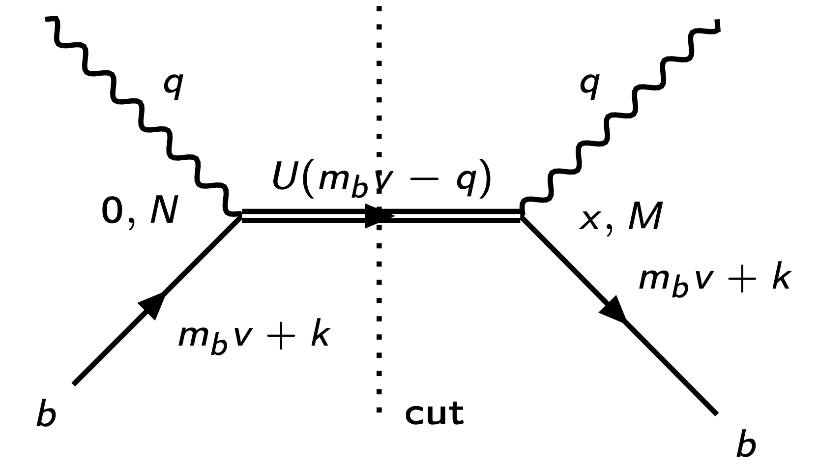
Figure 1: Discontinuity of the forward amplitude across the cut of the semileptonic process.

The hadron momentum $p=m_{b}\,v+k$ is written in terms of the 4-velocity $v$, the heavy quark mass $m_{b}$ and the residual momentum $k$, with $|k|\sim\mathcal{O}(\Lambda_{\text{QCD}})$. The QCD quark field $b(x)$ is redefined as $b(x)=e^{-i\,m_{b}\,v\cdot x}\,b_{v}(x)$, with $b_{v}(x)$ still QCD quark field satisfying the EoM $b_{v}(x)=\left(P_{+}+\frac{i\,\not{D}}{2\,m_{b}}\right)\,b_{v}(x)$, where $P_{\pm}=\frac{1\pm\not{v}}{2}$ are the velocity projectors.

Introducing $p_{X}=m_{b}\,v+k-q$, the Eq. (3) becomes

$$(T^{ij})_{MN}=\braket{H_{b}(v,s)}{\bar{b}_{v}(0)\,\overline{\Gamma}_{M}^{(i)}\,\frac{1}{\not{p}_{X}-m_{U}}\,\Gamma_{N}^{(j)}\,b_{v}(0)}{H_{b}(v,s)}\;,$$ (4)

and considering $|k|\sim\mathcal{O}(\Lambda_{\text{QCD}})$ we have

$$(T^{ij})_{MN}=\sum_{n=0}^{+\infty}\,\braket{H_{b}(v,s)}{\bar{b}_{v}(0)\,\overline{\Gamma}_{M}^{(i)}\,(\not{p}_{U}+m_{U})\,(i\,\not{D}\,(\not{p}_{U}+m_{U}))^{n}\,\Gamma_{N}^{(j)}\,b_{v}(0)}{H_{b}(v,s)}\,\frac{(-1)^{n}}{\Delta_{0}^{n+1}}\;,$$ (5)

where $\overline{\Gamma}_{M}^{(i)}=\gamma^{0}\,\Gamma_{M}^{(i)\dagger}\,\gamma^{0}$, $p_{U}=p_{X}-k$ and $\Delta_{0}=p_{U}^{2}-m_{U}^{2}$.

Using the trace formalism Dassinger:2006md , we can write the n-th term in the series as

$$\begin{split}&\braket{H_{b}(v,s)}{\bar{b}_{v}(0)\,\overline{\Gamma}_{M}^{(i)}\,(\not{p}_{U}+m_{U})\,\underbrace{i\,\not{D}\,(\not{p}_{U}+m_{U})\dots i\,\not{D}\,(\not{p}_{U}+m_{U})}_{\text{n times}}\,\Gamma_{N}^{(j)}\,b_{v}(0)}{H_{b}(v,s)}=\\ &=\bigg{[}\overline{\Gamma}_{M}^{(i)}\,(\not{p}_{U}+m_{U})\,\prod_{k=1}^{n}\,\left[\gamma_{\mu_{k}}\,(\not{p}_{U}+m_{U})\right]\,\Gamma_{N}^{(j)}\bigg{]}_{ab}\,\underbrace{\braket{H_{b}(v,s)}{\bar{b}_{v}(0)\,iD^{\mu_{1}}\,\dots\,iD^{\mu_{n}}\,b_{v}(0)}{H_{b}(v,s)}_{ba}}_{(\mathcal{M}^{\mu_{1}\dots\mu_{n}})_{ba}}\;.\end{split}$$ (6)

The expression in Eq. (6) involves the hadronic matrix elements $(\mathcal{M}^{\mu_{1}\dots\mu_{n}})_{ba}$ where $a$ and $b$ are Dirac indices. These matrix elements can be written in terms of nonperturbative parameters, the number of which increases with the order of the expansion:

$$\mathcal{O}(1/m_{b}^{n})\dots\begin{cases}\mathcal{O}(1/m_{b}^{3})\begin{cases}\mathcal{O}(1/m_{b}^{2})\begin{cases}-2\,M_{H}\,\hat{\mu}_{\pi}^{2}=\braket{H_{b}}{\bar{b}_{v}\,iD^{\mu}\,iD_{\mu}\,b_{v}}{H_{b}}\\ 2\,M_{H}\,\hat{\mu}_{G}^{2}=\braket{H_{b}}{\bar{b}_{v}\,(-i\sigma_{\mu\nu})\,iD^{\mu}\,iD^{\nu}\,b_{v}}{H_{b}}\end{cases}\\ 2\,M_{H}\,\hat{\rho}_{D}^{3}=\braket{H_{b}}{\bar{b}_{v}\,iD^{\mu}\,(iv\cdot D)\,iD_{\mu}\,b_{v}}{H_{b}}\\ 2\,M_{H}\,\hat{\rho}_{LS}^{3}=\braket{H_{b}}{\bar{b}_{v}\,(-i\sigma_{\mu\nu})\,iD^{\mu}\,(iv\cdot D)\,iD^{\nu}\,b_{v}}{H_{b}}\end{cases}\\ \dots\end{cases}\;.$$ (7)

To compute $\mathcal{M}^{\mu_{1}\dots\mu_{n}}$ one can follow the methods proposed in Dassinger:2006md ; Mannel:2010wj .
In the case of baryons, the dependence on the spin $s_{\mu}$ in Eq. (6) must be kept into account as done up to $\mathcal{O}(1/m_{b}^{-2})$ in Manohar:1993qn . In Colangelo:2020vhu $\mathcal{M}^{\mu_{1}\dots\mu_{n}}$ have been derived at $\mathcal{O}(1/m_{b}^{-3})$ for a polarized baryon, extending the previous results obtained in Mannel:2017jfk ; Kamali:2018bdp ; Grossman:1994ax ; Manohar:1993qn ; Balk:1997fg .

From the expressions of the matrix elements $\mathcal{M}^{\mu_{1}\dots\mu_{n}}$ the hadronic tensor can be computed and expanded in Lorentz structures which depend on $v$, $q$ and $s$. The results for the effective Hamiltonian Eq. (1) are collected in Colangelo:2020vhu . The four-fold differential decay rate for the $H_{b}(p,s)\to X_{U}(p_{X})\,\ell^{-}(p_{\ell})\,\bar{\nu}_{\ell}(p_{\nu})$ transition reads

$$\frac{\text{d}^{4}\Gamma}{\text{d}E_{\ell}\,\text{d}q^{2}\,\text{d}q_{0}\,\text{d}\cos\theta_{P}}=\frac{G_{F}^{2}\,|V_{Ub}|^{2}}{32\,(2\,\pi)^{3}\,M_{H}}\,\sum_{i,j}\,g_{i}^{*}\,g_{j}\,\frac{1}{\pi}\,\text{Im}\left[(T^{ij})_{MN}\right]\,(L^{ij})^{MN}\;,$$ (8)

where $p_{\ell}=(E_{\ell},\vec{p}_{\ell})$, $q_{0}=q\cdot v$ and $\theta_{P}$ is the angle between the two 3-vectors $\vec{p}_{\ell}$ and $\vec{s}$ in the $H_{b}$ rest frame. Double and single distributions are obtained integrating Eq. (8) over the phase-space Jezabek:1996ia . The full decay width can be obtained by performing all integrations and can be written as:

$$\Gamma(H_{b}\to X_{U}\,\ell^{-}\,\bar{\nu}_{\ell})=\Gamma_{b}\,\sum_{i,j}\,g_{i}^{*}\,g_{j}\,\,\left[\mathcal{C}_{0}^{(i,j)}+\frac{\hat{\mu}_{\pi}^{2}}{m_{b}^{2}}\,\mathcal{C}_{\hat{\mu}_{\pi}^{2}}^{(i,j)}+\frac{\hat{\mu}_{G}^{2}}{m_{b}^{2}}\,\mathcal{C}_{\hat{\mu}_{G}^{2}}^{(i,j)}+\frac{\hat{\rho}_{D}^{3}}{m_{b}^{3}}\,\mathcal{C}_{\hat{\rho}_{D}^{3}}^{(i,j)}+\frac{\hat{\rho}_{LS}^{3}}{m_{b}^{3}}\,\mathcal{C}_{\hat{\rho}_{LS}^{3}}^{(i,j)}\right]\;,$$ (9)

where $\Gamma_{b}=\frac{G_{F}^{2}\,|V_{Ub}|^{2}\,m_{b}^{5}}{192\,\pi^{3}}$ is the partonic term corresponding to a free quark decay. The indices $i$ and $j$ runs over the contributions of the various operators and of their interferences. The coefficients $\mathcal{C}^{(i,j)}$ can be found in Colangelo:2020vhu . The OPE breaks down in the endpoint region of the spectra, where singularities appear and which should be resummed in a $H_{b}$ shape function, the convolution with such a function smears the spectra at the endpoint. The effects of the baryon shape function has not been considered here. Perturbative QCD corrections have also been not included: in the SM case they can be found in Czarnecki:1994bn ; Jezabek:1996db ; DeFazio:1999ptt ; Trott:2004xc ; Aquila:2005hq ; Alberti:2014yda . NLO QCD corrections have also been recently computed in Mannel:2021zzr ; Moreno:2022goo .

4 Results for $\Lambda_{b}\to X_{c,u}\,\ell\,\bar{\nu}_{\ell}$

In Colangelo:2020vhu several observables for the modes $\Lambda_{b}\to X_{c,u}\,\ell\,\bar{\nu}_{\ell}$ have been studied. Here we consider a few of them. Further ones, as well as the input parameters, can be found in Colangelo:2020vhu . For the couplings $\epsilon_{i}^{\ell}$ in Eq. (1) we fix three NP benchmark points, set in Colangelo:2018cnj ; Shi:2019gxi for $U=c$, while for $U=u$ we use the ranges fixed in Colangelo:2019axi . Using $G_{F}=1.16637(1)\times 10^{-5}\,\text{GeV}^{-2}$, $|V_{cb}|=0.042$ and $|V_{ub}|=0.0037$, together with $\tau_{\Lambda_{b}}=1.471(9)\,\text{ps}$ Workman:2022ynf , we compute the inclusive $\Lambda_{b}$ branching fraction for the two quark transitions and for final $\tau$ and $\mu$ lepton. The results in the SM, for the central values of the parameters and neglecting QCD corrections, are in table 1.

Table 1: Inclusive semileptonic $\Lambda_{b}$ branching fractions in SM, obtained for the central values of the parameters.

$b\to c$		$b\to u$
$\mathcal{B}(\Lambda_{b}\to X_{c}\,\mu\,\bar{\nu}_{\mu})$	$11.0\times 10^{-2}$	$\mathcal{B}(\Lambda_{b}\to X_{u}\,\mu\,\bar{\nu}_{\mu})$	$11.65\times 10^{-4}$
$\mathcal{B}(\Lambda_{b}\to X_{c}\,\tau\,\bar{\nu}_{\tau})$	$2.4\times 10^{-2}$	$\mathcal{B}(\Lambda_{b}\to X_{u}\,\tau\,\bar{\nu}_{\tau})$	$2.75\times 10^{-4}$

For comparison, the available measurements are $\mathcal{B}(\Lambda_{b}\to\Lambda_{c}\,\ell^{-}\,\bar{\nu}_{\ell}+\text{anything})=(10.9\pm 2.2)\times 10^{-2}$, with $\ell=e,\mu$ and $\mathcal{B}(\Lambda_{b}\to p\,\mu^{-}\,\bar{\nu}_{\mu})=(4.1\pm 1.0)\times 10^{-4}$Workman:2022ynf .

For inclusive semileptonic $\Lambda_{b}$ decays it is interesting to consider a ratio analogous to $R{(D^{*})}$ for $B$ meson, to compare the $\tau$ and the muon mode using a quantity in which several theoretical uncertainties cancel:

$$R_{\Lambda_{b}}(X_{U})=\frac{\Gamma(\Lambda_{b}\to X_{U}\,\tau\,\bar{\nu}_{\tau})}{\Gamma(\Lambda_{b}\to X_{U}\,\mu\,\bar{\nu}_{\mu})}\qquad\text{with}\qquad U=u,c\;.$$ (10)

Another ratio sensitive to LFU violating NP effects can be defined. It can be constructed from the distribution $\frac{\text{d}\Gamma(\Lambda_{b}\to X_{U}\,\ell\,\bar{\nu}_{\ell})}{\text{d}\cos\theta_{P}}=A_{\ell}^{U}+B_{\ell}^{U}\,\cos\theta_{P}$. The dependence of $\frac{\text{d}\Gamma(\Lambda_{b}\to X_{U}\,\ell\,\bar{\nu}_{\ell})}{\text{d}\cos\theta_{P}}$ on $\cos\theta_{P}$ is linear, and NP contributions modify both the slope and the intercept of the curve as displayed in figure 2.

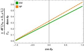
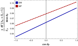
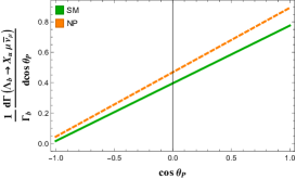
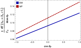
Figure 2: $\frac{1}{\Gamma_{b}}\,\frac{\text{d}\Gamma}{\text{d}\cos\theta_{P}}$ distribution for $\Lambda_{b}\to X_{U}\,\ell\,\bar{\nu}_{\ell}$, with $U=c$ (top row), $U=u$ (bottom row), $\ell=\mu$ (left column) and $\ell=\tau$ (right column). The solid line is the SM result, the dashed line the NP result at the benchmark point.

Similarly to the ratio defined in Eq. (10), we define the ratio of the slopes $R_{S}^{U}=B_{\tau}^{U}/B_{\mu}^{U}$ which has a definite value in SM, and can deviate due to NP as specified in table 2.

Table 2: Ratios $R_{\Lambda_{b}}(X_{u})$ and $R_{\Lambda_{b}}(X_{c})$ (left) and ratios $R_{S}^{u}$ and $R_{S}^{c}$ (right) for SM and NP at the BP.

	$R_{\Lambda_{b}}(X_{u})$	$R_{\Lambda_{b}}(X_{c})$	$R_{S}^{u}$	$R_{S}^{c}$
SM	$0.234$	$0.214$	$0.081$	$0.100$
NP	$0.238$	$0.240$	$0.091$	$0.074$

A correlation between $R_{\Lambda_{b}}(X_{U})$ and $R_{S}^{U}$ can be constructed. As an example, for $\Lambda_{b}\to X_{c}\,\tau\,\bar{\nu}_{\tau}$ with the effective Hamiltonian extended including a tensor operator, we vary the couplings $\big{(}\text{Re}[\epsilon_{T}^{\mu}],\text{Im}[\epsilon_{T}^{\mu}]\big{)}$ and $\big{(}\text{Re}[\epsilon_{T}^{\tau}],\text{Im}[\epsilon_{T}^{\tau}]\big{)}$ in the regions determined in Colangelo:2018cnj . The correlation plot in figure 3 shows that the (challenging) measurement of the two ratios would discriminate SM and NP.

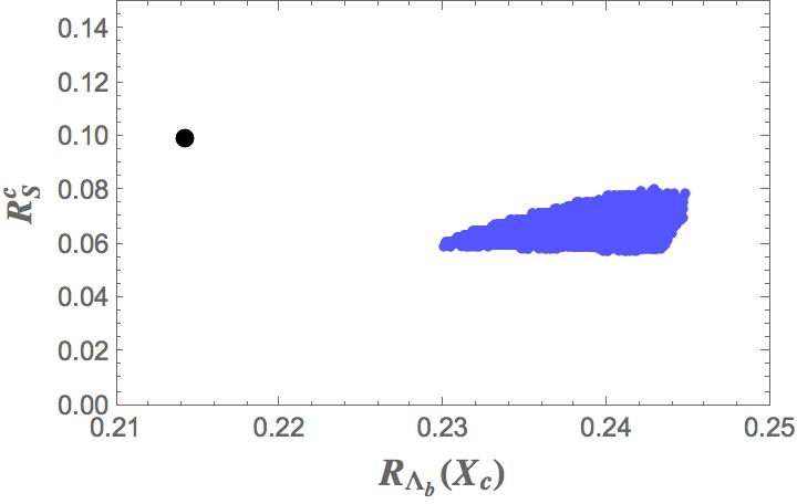
Figure 3: Correlation between $R_{\Lambda_{b}}(X_{c})$ and the ratio $R_{S}^{c}$ of the slopes of the $\frac{\text{d}\Gamma}{\text{d}\cos\theta_{P}}$ distribution. The dot corresponds to SM, the broad region to NP with the effective couplings varied as specified in the text.

5 Conclusions

The calculation of the fully differential inclusive semileptonic decay width of a polarized heavy hadron at $\mathcal{O}(1/m_{b}^{3})$ in the HQE, at leading order in $\alpha_{s}$ and for non vanishing charged lepton mass has been described. NP generalization of the SM has been considered in the effective Hamiltonian in Eq.(1) including all the $D=6$ semileptonic operators with left-handed neutrinos. The correlation plot in figure 3 shows that the ratios $R_{\Lambda_{b}}(X_{c})$ and $R_{S}^{c}$ can assume different values in the SM and when NP is included. Although this measurement is experimentally challenging, it represents a suitable observable to test violation of LFU.

References

- (1) S. Fajfer, J.F. Kamenik, I. Nisandzic, Phys. Rev. D85, 094025 (2012), 1203.2654
- (2) M. Algueró, B. Capdevila, S. Descotes-Genon, J. Matias, M. Novoa-Brunet, global fits after Moriond 2021 results, in 55th Rencontres de Moriond on QCD and High Energy Interactions (2021), 2104.08921
- (3) P. Colangelo, F. De Fazio, F. Loparco, JHEP 11, 032 (2020), 2006.13759
- (4) I.I.Y. Bigi, M.A. Shifman, N.G. Uraltsev, A.I. Vainshtein, Phys. Rev. Lett. 71, 496 (1993), hep-ph/9304225
- (5) J. Chay, H. Georgi, B. Grinstein, Phys. Lett. B 247, 399 (1990)
- (6) P. Biancofiore, P. Colangelo, F. De Fazio, Phys. Rev. D87, 074010 (2013), 1302.1042
- (7) P. Colangelo, F. De Fazio, JHEP 06, 082 (2018), 1801.10468
- (8) S. Bhattacharya, S. Nandi, S. Kumar Patra, Eur. Phys. J. C 79, 268 (2019), 1805.08222
- (9) P. Colangelo, F. De Fazio, Phys. Rev. D95, 011701 (2017), 1611.07387
- (10) T. Mannel, A.V. Rusov, F. Shahriaran, Nucl. Phys. B 921, 211 (2017), 1702.01089
- (11) S. Kamali, A. Rashed, A. Datta, Phys. Rev. D 97, 095034 (2018), 1801.08259
- (12) S. Kamali, Int. J. Mod. Phys. A 34, 1950036 (2019), 1811.07393
- (13) D. Moreno (2022), 2207.14245
- (14) R. Aaij et al. (LHCb), Phys. Lett. B 724, 27 (2013), 1302.5578
- (15) G. Aad et al. (ATLAS), Phys. Rev. D 89, 092009 (2014), 1404.1071
- (16) A.M. Sirunyan et al. (CMS), Phys. Rev. D 97, 072010 (2018), 1802.04867
- (17) R. Aaij et al. (LHCb), JHEP 06, 110 (2020), 2004.10563
- (18) D. Buskulic et al. (ALEPH), Phys. Lett. B 365, 437 (1996)
- (19) G. Abbiendi et al. (OPAL), Phys. Lett. B 444, 539 (1998), hep-ex/9808006
- (20) P. Abreu et al. (DELPHI), Phys. Lett. B 474, 205 (2000)
- (21) B.M. Dassinger, T. Mannel, S. Turczyk, JHEP 03, 087 (2007), hep-ph/0611168
- (22) T. Mannel, S. Turczyk, N. Uraltsev, JHEP 11, 109 (2010), 1009.4622
- (23) A.V. Manohar, M.B. Wise, Phys. Rev. D 49, 1310 (1994), hep-ph/9308246
- (24) Y. Grossman, Z. Ligeti, Phys. Lett. B 332, 373 (1994), hep-ph/9403376
- (25) S. Balk, J.G. Korner, D. Pirjol, Eur. Phys. J. C 1, 221 (1998), hep-ph/9703344
- (26) M. Jezabek, L. Motyka, Acta Phys. Polon. B 27, 3603 (1996), hep-ph/9609352
- (27) A. Czarnecki, M. Jezabek, J.H. Kuhn, Phys. Lett. B 346, 335 (1995), hep-ph/9411282
- (28) M. Jezabek, L. Motyka, Nucl. Phys. B 501, 207 (1997), hep-ph/9701358
- (29) F. De Fazio, M. Neubert, JHEP 06, 017 (1999), hep-ph/9905351
- (30) M. Trott, Phys. Rev. D 70, 073003 (2004), hep-ph/0402120
- (31) V. Aquila, P. Gambino, G. Ridolfi, N. Uraltsev, Nucl. Phys. B 719, 77 (2005), hep-ph/0503083
- (32) A. Alberti, P. Gambino, K.J. Healey, S. Nandi, Phys. Rev. Lett. 114, 061802 (2015), 1411.6560
- (33) T. Mannel, D. Moreno, A.A. Pivovarov, Phys. Rev. D 105, 054033 (2022), 2112.03875
- (34) R.X. Shi, L.S. Geng, B. Grinstein, S. Jäger, J. Martin Camalich, JHEP 12, 065 (2019), 1905.08498
- (35) P. Colangelo, F. De Fazio, F. Loparco, Phys. Rev. D 100, 075037 (2019), 1906.07068
- (36) R.L. Workman (Particle Data Group), PTEP 2022, 083C01 (2022)