Normal approximation for the posterior in exponential families

Abstract

In this paper we obtain quantitative Bernstein-von Mises type bounds on the normal approximation of the posterior distribution in exponential family models when centering either around the posterior mode or around the maximum likelihood estimator. Our bounds, obtained through a version of Stein’s method, are non-asymptotic, and data dependent; they are of the correct order both in the total variation and Wasserstein distances, as well as for approximations for expectations of smooth functions of the posterior. All our results are valid for univariate and multivariate posteriors alike, and do not require a conjugate prior setting. We illustrate our findings on a variety of exponential family distributions, including Poisson, multinomial and normal distribution with unknown mean and variance. The resulting bounds have an explicit dependence on the prior distribution and on sufficient statistics of the data from the sample, and thus provide insight into how these factors may affect the quality of the normal approximation.

Keywords: Exponential family; posterior distribution; prior distribution; Bayesian inference; normal approximation; Stein’s method

AMS 2010 Subject Classification: Primary 60F05; 62E17; Secondary 62F10; 62F15

1 Introduction

The Bernstein-von Mises (BvM) Theorem is a cornerstone in Bayesian statistics. Loosely put, this theorem reconciles Bayesian and frequentist large sample theory by guaranteeing that suitable scalings of posterior distributions are asymptotically normal. In particular, this implies that the contribution of the prior vanishes in the asymptotic posterior. There exist many different versions of the BvM Theorem; here we consider the following setting. Let $\theta\sim\pi_{0}$ follow the prior distribution, and conditional on $\theta$ let $X_{1},\ldots,X_{n}$ be independent and identically distributed (i.i.d.) random variables from the model $P_{\theta}$. Let $p_{2}(\theta|x_{1},\ldots,x_{n})$ denote the posterior distribution of $\theta$ given $X_{i}=x_{i}$, $i=1,\ldots,n$; it is assumed that the posterior density is differentiable and vanishes on the boundary of its support. Let $\tilde{\theta}$ denote the posterior mode of $\theta$. The BvM Theorem then assures us that, under regularity conditions, the posterior distribution of $\theta$ can be well approximated by a normal distribution with mean $\tilde{\theta}$ and covariance $J^{-1}(\tilde{\theta})$ where $J(\tilde{\theta})$ denotes the observed Fisher information matrix. Another standard formulation is based on the maximum likelihood estimate (MLE) $\hat{\theta}$: under appropriate regularity conditions, the posterior is similarly well approximated by a $N(\hat{\theta},J^{-1}(\hat{\theta}))$ distribution. Note how in both versions of the statement, the parameters of the approximating normal distribution typically depend on the observed data. More generally, the centering and scaling can be performed around any consistent estimator of the true parameter.

The literature on the BvM Theorem is vast, and we will provide a brief overview at the end of this introduction. A common trait of many recent references on the topic is the need for non-asymptotic (i.e. finite sample) bounds which detail the impact of the model specificities on the quality of the approximation. In this paper, we revisit this question under the classical assumption that the data are i.i.d. observations from a regular $k$-parameter exponential family ($k\geq 1$). We provide quantitative bounds to assess the approximation of the posterior by the $N(\tilde{\theta},J^{-1}(\tilde{\theta}))$ and $N(\hat{\theta},J^{-1}(\hat{\theta}))$ distributions. Our bounds are given with respect to the total variation and Wasserstein distances, and we also give approximations for expectations of smooth functions of the posterior. Under suitable assumptions on the data, our bounds are of the optimal order $n^{-1/2}$. For total variation distance we are also able to provide $O(n^{-1/2})$ bounds that hold under weaker local assumptions. From these bounds we infer that only the behaviour of the posterior distribution in a ‘small’ neighbourhood of the posterior mode or MLE (depending on the standardisation used) is relevant to the rate of convergence in total variation distance, provided the posterior satisfies a certain integrability condition. Moreover, when our general bounds are applied in concrete examples, they have an explicit dependence on the parameters of the prior distribution, on sufficient statistics of the data, as well as on the dimension $k$. Such explicit bounds provide new insight into the characteristics of the model that are most prevalent in determining the rate of convergence of the posterior to its asymptotic normal distribution.

Our main tool is the “comparison of Stein operators” method initiated in [42], and developed in [28, 32]. As is well-known, Charles Stein’s operator theory allows to characterize distributions in terms of objects which do not depend on the underlying normalising constants – this is crucial to the success of our approach. The second crucial element is the exponential family assumption, which allows us to write many of our results in terms of explicit quantities. Writing out the bounds in a multivariate context necessitates relatively heavy notations which obfuscate the underlying simplicity of the approach. To give the reader intuition on our method, we begin by illustrating our approach in the one-dimensional setting.

1.1 Finite sample BvM-type bounds for univariate exponential families

Fix an integer $n\geq 1$ and let $\mathbf{x}=(x_{1},\ldots,x_{n})$ be i.i.d. observations from a regular exponential family in natural parametrisation $p_{1}(x\,|\,\theta)=\mathrm{exp}\left(\theta h(x)-g(x)-\beta(\theta)\right)$, where $\theta\in\Theta\subset\mathbb{R}$ is the parameter of interest, and the functions $g,\beta$ ensure that $p_{1}(\cdot\,|\,\theta)$ is a density (with respect to some dominating measure) whose support does not depend on $\theta$. Given some (possibly improper) differentiable prior $\pi_{0}(\theta)$, let $\eta(\theta)=-\log\pi_{0}(\theta)$ and consider

$$p_{2}(\theta\,|\,\mathbf{x})\propto\mathrm{exp}\left(\theta\sum_{i=1}^{n}h(x_{i})-n\beta(\theta)-\eta(\theta)\right)=:\mathrm{exp}\left(\theta\sum_{i=1}^{n}h(x_{i})-\lambda(\theta)\right)$$

the density (with respect to the Lebesgue measure) of the corresponding posterior distribution. Suppose that the posterior density is unimodal with mode $\tilde{\theta}=(\lambda^{\prime})^{-1}(\sum_{i=1}^{n}h(x_{i}))$. Letting $\theta\sim p_{2}(\cdot\,|\,\mathbf{x})$, our objective is to provide fixed-sample, data dependent, and explicit bounds on quantities of the form

$$d_{\mathcal{H}}(\theta^{\star},N)=\sup_{h\in\mathcal{H}}|\mathbb{E}[h(\theta^{\star})]-\mathbb{E}[h(N)]|,$$

where $\theta^{\star}=(\lambda^{\prime\prime}(\tilde{\theta}))^{1/2}(\theta-\tilde{\theta})$, $N\sim N(0,1)$, and $\mathcal{H}$ is a measure-separating collection of functions which are integrable with respect to both $\theta^{\star}$ and $N$. Here, and throughout the paper, we use a standard abuse of notation that $d_{\mathcal{H}}(X,Y)$ represents $d_{\mathcal{H}}(P,Q)$, where $P$ and $Q$ are the probability measures of $X$ and $Y$. Probability distances of this form, in the general multivariate setting, are called Integral Probability Metrics (IPMs) and include, among many others, (i) the total variation distance $d_{\mathrm{TV}}$ obtained from $\mathcal{H}_{\mathrm{TV}}=\{\mathbb{I}[\cdot\in A]\,:\,A\subset\mathcal{B}(\mathbb{R}^{k})\}$, and (ii) the Wasserstein (a.k.a. Kantorovitch) distance $d_{\mathrm{Wass}}$ obtained from $\mathcal{H}_{\mathrm{Wass}}=\{h:\mathbb{R}^{k}\rightarrow\mathbb{R}\,:\,h\text{is Lipschitz},\|h\|_{\mathrm{Lip}}\leq 1\}$. Here $\mathcal{B}(\mathbb{R}^{k})$ denotes the Borel $\sigma$-algebra on $\mathbb{R}^{k}$ and $\|h\|_{\mathrm{Lip}}:=\sup_{x\not=y}|h(x)-h(y)|/\|x-y\|_{2}$, where $\|\cdot\|_{2}$ is the Euclidean distance on $\mathbb{R}^{k}$. Of course any total variation bound ensures a bound in Kolmogorov distance (because the supremum is taken over a smaller set); any Wasserstein bound provides bounds on the differences of the expectations.

Stein’s method is very well-suited for bounding IPMs. In the present context, the approach can be described as follows (see Section 4 for a more in-depth overview and references). For $h\in\mathcal{H}$, let $f_{h}(x)=e^{x^{2}/2}\int_{-\infty}^{x}(h(u)-\mathbb{E}[h(N)])e^{-u^{2}/2}du$. This function is differentiable, and satisfies $f_{h}^{\prime}(x)-xf_{h}(x)=h(x)-\mathbb{E}[h(N)]$ for all $x\in\mathbb{R}$. Hence $\mathbb{E}[h(\theta^{\star})]-\mathbb{E}[h(N)]=\mathbb{E}[f_{h}^{\prime}(\theta^{\star})-\theta^{\star}f_{h}(\theta^{\star})]$. Next let $p^{\star}_{2}(\cdot\,|\,\mathbf{x})$ denote the density of $\theta^{\star}$. Then one easily proves via a Fubini argument that $\mathbb{E}[f_{h}^{\prime}(\theta^{\star})]=-\mathbb{E}[f_{h}(\theta^{\star})\log(p_{2}(\theta^{\star}\,|\,\mathbf{x}))^{\prime}]$ as long as $p_{2}^{\star}(\cdot\,|\,\mathbf{x})$ vanishes at the boundary of its support. From our assumptions on the model, the derivative of the log likelihood of the standardised posterior takes on a very simple form, so that after some straightforward simplifications we obtain $\mathbb{E}[h(\theta^{\star})]-\mathbb{E}[h(N)]=\lambda^{\prime\prime}(\tilde{\theta})^{-1/2}\mathbb{E}[f_{h}(\theta^{\star})(\lambda^{\prime}(\theta)-\lambda^{\prime}(\tilde{\theta})-\lambda^{\prime\prime}(\tilde{\theta})(\theta-\tilde{\theta}))]$ and thus

$$d_{\mathcal{H}}(\theta^{\star},N)\leq C(\mathcal{H})\Delta,$$

where

$$C(\mathcal{H})=\sup_{h\in\mathcal{H}}\|f_{h}\|_{\infty}\mbox{ and }\Delta(=\Delta(\mathbf{x}))=\lambda^{\prime\prime}(\tilde{\theta})^{-1/2}\mathbb{E}\left[\left|\lambda^{\prime}(\theta)-\lambda^{\prime}(\tilde{\theta})-\lambda^{\prime\prime}(\tilde{\theta})(\theta-\tilde{\theta})\right|\right].$$

The constants $C(\mathcal{H})$ can be bounded explicitly and uniformly for many choices of classes of test functions $\mathcal{H}$. In particular $C(\mathcal{H}_{\mathrm{TV}})=\sqrt{\pi/8}$ and $C(\mathcal{H}_{\mathrm{Wass}})=1$ (see e.g. [14]). Hence proximity in total variation distance, in Wasserstein distance (or, for that matter, in any other IPM $d_{\mathcal{H}}(\theta^{\star},N)$ such that $C(\mathcal{H})<\infty$) is entirely controlled by the data-dependent quantity $\Delta$. A similar tale can also be told when centering around the MLE $\hat{\theta}=(\beta^{\prime})^{-1}(\sum_{i=1}^{n}h(x_{i}))$, leading to similarly flavored bounds on the resulting IPMs (with a slight but obvious modification of the leading term $\Delta$).

It remains to transform this finding into meaningful bounds. If, for instance, $\|\lambda^{\prime\prime\prime}\|_{\infty}<\infty$ (we shall see in Example 1 that this is the case for Bernoulli data with conjugate prior) then a straightforward Taylor expansion yields $\mathbb{E}[|\lambda^{\prime}(\theta)-\lambda^{\prime}(\tilde{\theta})-\lambda^{\prime\prime}(\tilde{\theta})(\theta-\tilde{\theta})|]\leq\|\lambda^{\prime\prime\prime}\|_{\infty}\mathbb{E}[(\theta-\tilde{\theta})^{2}]$ so that the proximity between $\theta^{\star}$ and $N$ in any IPM with finite $\mathcal{C}(\mathcal{H})$ is now entirely computable as an explicit function of the sufficient statistic $\sum_{i=1}^{n}h(x_{i})$ and of the parameters of the model; a similar argument carries through when centering around the MLE. Other adhoc assumptions (strict-convexity of $\lambda^{\prime}$, polynomial growth for $\lambda^{\prime\prime\prime}$, etc.) will also lead to precise bounds. We however aim to propose more general and easy-to-apply bounds which do not require such assumptions. As we shall see, the general setting requires some more careful analysis – such is the purpose of this paper.

1.2 Related work

Let us return to the general (multivariate) setting. If we assume that the true underlying distribution is $P_{\theta_{0}}$, and let $\overline{\theta}_{n}$ be any sequence of asymptotically efficient estimators, then the classical BvM theorem states that, under mild assumptions on the likelihood and the prior, the total variation distance between the law of $\sqrt{n}(\theta-\overline{\theta}_{n})$ and the centered normal law with variance $J(\theta_{0})$ converges to 0 in probability (with respect to the law of the data) as the sample size grows to infinity; see e.g. [43, Section 10.2]. Asymptotic normality of the posterior still holds, though obviously with a different limiting covariance matrix, if we no longer suppose the true underlying distribution $P_{0}$ to be of the form $P_{\theta_{0}}$ that is, if we consider a misspecified model setting; see e.g.  [6] where the result is obtained under a Local Asymptotic Normality (LAN) condition. We refer to [7] for an overview along with an up-to-date reference list, both in the specified and in the misspecified settings; see also [33] for almost sure versions of these statements. Semiparametric BvM theorems have also been obtained e.g. in [6] (still under a LAN condition), or in [10] for smooth functionals, both for i.i.d. and non-i.i.d. samples. Finally, we mention that versions of the BvM result also hold true in nonparametric settings (see e.g. [9]) or high-dimensional settings, see [25]. We refer to [37] for an overview. This is but a partial and biased snippet of a very large body of work; we have not aimed at being exhaustive.

A common trait of the BvM statements from the above references is that they are provided in terms of the asymptotic behavior of the random variable $d_{\mathrm{TV}}(\theta^{\star},N)$. In practice, however, there is a need for non-asymptotic (i.e. fixed sample) statements which, arguably, are of a different nature. Here, and as already described in the univariate case in the previous section, the objective is to study for fixed sample $\mathbf{x}$ the proximity between the standardised posterior distribution (conditioned on the observation) and a standard normal distribution. An important reference on this topic is [34] where such a finite sample semiparametric version of the BvM theorem is obtained for non-informative and flat Gaussian priors. Similar spirited fixed sample bounds are also obtained in [40] for Gaussian priors in high-dimensional or nonparametric setups, while [39] considers Gaussian priors and log-concave likelihoods. In the last two mentioned references, the bounds are also expressed in terms of the Kolmogorov distance. Reference [44] obtains Berry–Esseen type bounds for the BvM theorem (here expressed in total variation distance) for inference on the slope vector in approximately linear regression models. Again, this is but a snapshot of a very active field of research. Among the recent productions we highlight the preprint [26] which provides results closest in spirit to ours. Here, a (very different) version of Stein’s method is used to obtain fixed-sample BvM theorems for general prior and general likelihood, under regularity conditions (local growth condition on the third derivative of the likelihood, non-vanishing prior bounded from above with bounded score function on a neighborhood of the centering, …). Aside from such regularity conditions, no assumption on the model is made. The cost of working at this a level of generality is paid both in terms of the transparency of the bounds and, also, their sharpness when applied to specific examples that can be related to ours. We will provide more comparisons in our examples section. [26] contains an excellent comparative overview of the state-of-the-art on fixed sample BvM theorems.

1.3 Structure of the paper

The rest of the paper is structured as follows. In Section 2, we state our main results. In Section 2.1, we give bounds for a standardisation of the posterior involving the posterior mode. Theorem 1 provides explicit order $n^{-1/2}$ bounds for the multivariate normal approximation of the posterior distribution in multi-parameter exponential family models in the total variation and Wasserstein distances. A useful alternative bound in the total variation metric, that holds under weaker local assumptions, is given in Theorem 2, whilst improved total variation distance bounds for the single-parameter case are given in Theorem 4. An abstract approximation for expectations of smooth functions of the posterior is given in Theorem 3 (a special case of this theorem yields bounds on the variance of the posterior). In Section 2.2, we give analogues of the bounds of Section 2.1 for a standardisation of the posterior involving the MLE. In Section 3, we apply our general bounds in several concrete examples, and provide some simulation results to assess performance. The proofs of our main results are given in Section 4. Some technical proofs are given in Appendix A. Further computations for the examples of Section 3 are given in the Supplementary Material.

2 Main Results

Let $n,k$ and $d$ be positive integers. Let ${\bf X}=(X_{1},\ldots,X_{n})$ be a vector of $n$ independent random vectors, each in $\mathbb{R}^{d}$, from a regular $k$-parameter exponential family, each $X_{i}$ with probability density $p_{1,i}(x\,|\,\theta)$ (with respect to some positive, $\sigma$-finite dominating measure $\mu_{i}$ defined on the Borel sets of $\mathbb{R}^{d}$) given in the canonical parametrisation (or canonical form),

$$p_{1,i}(x\,|\,\theta)=\mathrm{exp}\Bigg{(}\sum_{u=1}^{k}\theta_{u}h_{i,u}(x)-g_{i}(x)-\beta_{i}(\theta)\Bigg{)},$$ (1)

where $\theta=(\theta_{1},\ldots,\theta_{k})^{\intercal}$ is the parameter of interest which we suppose to belong to an open subset $\Theta\subseteq\mathbb{R}^{k}$. We do not assume that the $X_{i}$ are identically distributed; however, we assume that all $p_{1,i}(\cdot\,|\,\theta)$, have the same support $\mathcal{X}\subseteq\mathbb{R}^{d}$ which does not depend on $\theta$; the corresponding support indicator function is thus incorporated in the functions $g_{i}:\mathbb{R}^{d}\to\mathbb{R}$. We also assume that for all $i=1,\ldots,n$ the functions $h_{i,u}:\mathbb{R}^{d}\to\mathbb{R},\,u=1,\ldots,k$, are chosen so that the normalising constants $\mathrm{exp}(\beta_{i}(\theta))=\int\mathrm{exp}\big{(}\sum_{u=1}^{k}\theta_{u}h_{i,u}(x)-g_{i}(x)\big{)}\,d\mu(x)$ are finite. We remark that it is analytically convenient to work with exponential family distributions in canonical form, and that this comes with no loss of generality as any exponential family distribution can be reduced to the canonical form via a re-parametrisation. Finally, we note that, in $k$-parameter exponential family models, the statistic $t({\bf X})=(n,\sum_{i=1}^{n}h_{i,1}(X_{i}),\ldots,\sum_{i=1}^{n}h_{i,k}(X_{i}))$ is sufficient for $\theta$. The bounds in the examples of Section 3 are expressed in terms of the components of this statistic. More information about posteriors in exponential families can be found for example in [12].

Next, let ${\bf x}=(x_{1},\ldots,x_{n})$ be a fixed observation from the model and fix a possibly improper prior $\pi_{0}$ on the Borel subsets of $\mathbb{R}^{k}$, which, for notational convenience, we write as $\pi_{0}(\theta)=\mathrm{exp}(-\eta(\theta))$ for $\eta$ a scalar function on which appropriate assumptions will be imposed below. The posterior distribution given $\mathbf{x}$ is then

$$p_{2}(\theta|\mathbf{x})=\kappa(\mathbf{x})\exp\Bigg{(}\sum_{u=1}^{k}\theta_{u}\sum_{i=1}^{n}h_{i,u}(x_{i})-\sum_{i=1}^{n}\beta_{i}(\theta)-\eta(\theta)\Bigg{)},$$ (2)

where $\kappa(\mathbf{x})=\int_{\Theta}\Pi_{i=1}^{n}p_{1,i}(x_{i}\,|\,\theta)\pi_{0}(\theta)d\theta$ is the normalising constant. For $\beta_{i}(\cdot)$ and $\eta(\cdot)$ as in (2) we set

$$\lambda(\theta)=\sum_{i=1}^{n}\beta_{i}(\theta)+\eta(\theta),$$

and let $\mathbf{H}_{\lambda}$ denote its Hessian matrix, i.e. $\mathbf{H}_{\lambda}(\theta)$ is the $k\times k$ matrix with entries $(\mathbf{H}_{\lambda}(\theta))_{u,v}=\partial_{u,v}\lambda(\theta)$, $1\leq u,v\leq k$ (with $\partial_{u}=\frac{\partial}{\partial\theta_{u}}$ denoting the partial derivative with respect to the $u$th coordinate of $\theta$).

From now on we make the following standing assumption on the posterior distribution; this assumption will not be re-stated in our results as it is invariably assumed to hold.

Assumption 0

The posterior density $p_{2}(\theta|{\bf{x}})$ is differentiable and vanishes when $\theta$ approaches the boundary of its support.

Assumption 0 ensures that all integration by parts can be carried out without boundary terms since the functions we integrate against are always bounded; this assumption could obviously be weakened. As the approximating normal distribution naturally satisfies Assumption 0, for asymptotic normality such additional boundary terms will vanish in the limit even when Assumption 0 does not hold for finite $n$.

2.1 Bounds for standardisation based on the posterior mode

For a normal approximation based on the standardisation of the posterior distribution by the posterior mode we rely on the following (classical) assumptions.

Assumption $\widetilde{\textrm{A}}$

• The parameter $\theta$ is identifiable, in the sense that the map $\theta\mapsto p_{1}(\cdot|\theta)$ is one-to-one. The parameter space $\Theta$ is convex.

• The posterior mode $\tilde{\theta}$ is unique and is an interior point of $\Theta$.

• All third-order partial derivatives of $\lambda$ exist.

• The matrix $\mathbf{H}_{\lambda}(\tilde{\theta})$ is positive definite.

We note that the posterior mode depends on the data, and hence assumptions (A2), (A3) and (A4) depend implicitly on the data. Our formulation of the assumptions is required in the forthcoming proofs; weaker formulations exist, see e.g.  [43].

As noted by [31], in the single-parameter ($k=1$) case, a simple sufficient condition under which the posterior mode is unique is that the derivative $\lambda^{\prime}$ is an increasing function (and it then follows that $\tilde{\theta}=(\lambda^{\prime})^{-1}(\sum_{i}h_{i}(x_{i}))$). No such explicit condition or expression is available in general; however, upon noting that $\log p_{2}(\theta\,|\,\mathbf{x})=\sum_{{u=1}}^{k}\theta_{u}\sum_{i=1}^{n}h_{i,u}(x_{i})-\lambda(\theta)+{\log\kappa(\mathbf{x})}$, we immediately deduce the following fact (which we label for ease of future reference).

Fact 1a: The posterior mode $\tilde{\theta}$ solves the system of equations $\partial_{u}\lambda(w)-\sum_{i=1}^{n}h_{i,u}(x_{i})=0$, $u=1,\ldots,k$.

By definition, $\tilde{\theta}$ is a local maximum of $\log p_{2}(\theta\,|\,\mathbf{x})$, and thus $\mathbf{H}_{\lambda}(\tilde{\theta})$ must be positive semi-definite by the second derivative test. Assumption (A3) implies that all second-order partial derivatives of $\lambda$ are continuously differentiable, implying that, by Schwarz’s theorem, $\partial_{u,v}\lambda(\theta)=\partial_{v,u}\lambda(\theta)$ for all $1\leq u,v\leq k$ and all $\theta\in\mathbb{R}^{k}$. Thus, $\mathbf{H}_{\lambda}(\tilde{\theta})$ is a symmetric matrix. This implies that $\mathbf{H}_{\lambda}(\tilde{\theta})$ has a unique positive semi-definite square root, which we shall denote by $(\mathbf{H}_{\lambda}(\tilde{\theta}))^{1/2}$. Moreover, Assumption (A4) now implies that $\mathbf{H}_{\lambda}(\tilde{\theta})$ is invertible with inverse $(\mathbf{H}_{\lambda}(\tilde{\theta}))^{-1}$ which is also positive definite and therefore also has a unique positive definite square root, which we denote by $(\mathbf{H}_{\lambda}(\tilde{\theta}))^{-1/2}$.

In this subsection, we quantify, for a fixed observation $\mathbf{x}$, the proximity to the standard normal distribution of the distribution of the random vector

$$\theta^{\star}(=\theta^{\star}(\mathbf{x}))=(\mathbf{H}_{\lambda}(\tilde{\theta}))^{1/2}\big{(}\theta-\tilde{\theta}\big{)},$$ (3)

which is distributed according to the standardised posterior distribution centred at the posterior mode. Key quantities in all our bounds will be the scalars

$$R_{u}^{\lambda}(=R_{u}^{\lambda}(\mathbf{x}))=\bigg{|}\sum_{v=1}^{k}(\mathbf{H}_{\lambda}(\tilde{\theta}))^{-1/2})_{u,v}\bigg{|}\mbox{ and }\tilde{R}_{u}^{\lambda}(=\tilde{R}_{u}^{\lambda}(\mathbf{x}))=\sum_{v=1}^{k}|(\mathbf{H}_{\lambda}(\tilde{\theta}))^{-1/2})_{u,v}|,\quad u=1,\ldots,k,$$ (4)

as well as the functions $\tilde{\Upsilon}^{\lambda}_{l,u,v}:\mathbb{R}^{k}\to\mathbb{R}$ given for $1\leq l,u,v\leq k$ by

$$\tilde{\Upsilon}^{\lambda}_{l,u,v}(w)(=\tilde{\Upsilon}^{\lambda}_{l,u,v}(\mathbf{x},w))=\mathbb{E}\left[Y_{2}\partial_{l,u,v}\lambda\left(Y_{1}Y_{2}\big{(}\mathbf{H}_{\lambda}(\tilde{\theta})\big{)}^{-1/2}w+\tilde{\theta}\right)\right],$$ (5)

where here and throughout $Y_{1},Y_{2}$ are two uniform random variables on $(0,1)$, independent of each other and of all randomness involved. Throughout the paper, the notation $N$ is reserved for a standard normal random variable of the appropriate dimension.

Theorem 1.

Suppose that Assumption $\widetilde{\mathrm{A}}$ holds and, for $\theta^{\star}=(\theta^{\star}_{1},\ldots,\theta^{\star}_{k})^{\intercal}$ as in (3), set

$$\tilde{\Delta}_{\lambda}(=\tilde{\Delta}_{\lambda}(\mathbf{x}))=\sum_{l=1}^{k}\sum_{u=1}^{k}\sum_{v=1}^{k}\tilde{R}_{l}^{\lambda}R_{u}^{\lambda}R_{v}^{\lambda}\mathbb{E}\left[\left|\theta^{\star}_{u}\theta^{\star}_{v}\tilde{\Upsilon}^{\lambda}_{l,u,v}(\theta^{\star})\right|\right].$$ (6)

Then

$$d_{\mathrm{TV}}(\theta^{\star},N) \leq\frac{\sqrt{8\pi}}{3}\tilde{\Delta}_{\lambda}\mbox{ and }d_{\mathrm{Wass}}(\theta^{\star},N)\leq\tilde{\Delta}_{\lambda}.$$ (7)

Remark 1.

As $\lambda(w)=\sum_{i=1}^{n}\beta_{i}(w)+\eta(w)$, in ‘typical’ situations the row sums in (4) are of order $n^{-1/2}$, and we infer that the bounds of Theorem 1 are of order $n^{-1/2}$ for large $n$. Here and in the rest of the paper, the notion of order $n^{-1/2}$ has the following interpretation: the quantity of interest is of order $n^{-1/2}$ for ‘typical’ realisations of the data $\mathbf{x}$. ‘Typical’ is a loose term to indicate that the posterior mode (and the maximum likelihood estimator in the next section) are bounded sufficiently far away from the boundary of the parameter space as $n\rightarrow\infty$.

As an illustration, consider forthcoming Example 2, which concerns a conjugate prior for i.i.d. Poisson data $x_{1},\ldots,x_{n}$ with parameter $\mu$ and natural parameter $\theta=\log\mu$. Using our bounds we shall obtain $d_{\mathrm{TV}}(\theta^{\star},N)\leq 2.67\mathbb{E}[(\theta^{\star})^{2}]/\sqrt{\tau_{1}+n\bar{x}}$, where $\bar{x}=n^{-1}\sum_{i=1}^{n}x_{i}$ and $\tau_{1}>0$ is a prior parameter. According to our terminology, we would say that this bound is of order $n^{-1/2}$, as for a typical realisation of the data we would have that $n\bar{x}=O(n)$ for large $n$. However, for large finite $n$, with low probability, it is possible that $n\bar{x}=o(n)$, in which case, for this atypical data the bound decays slower than order $n^{-1/2}$. This behaviour of slower convergence rates for atypical data is to be expected, because, to take an extreme example in which $x_{1}=\cdots=x_{n}=0$ (for which our bound is $O(1)$), we have $\tilde{\theta}=\log(\tau_{1}/(n+\tau_{2}))$ and $\lambda(\tilde{\theta})=\tau_{1}$, and so $\theta^{\star}=\sqrt{\tau_{1}}(\theta-\log(\tau_{1}/(n+\tau_{2})))$ is not approximately $N(0,1)$ distributed for large $n$.

Expression $\tilde{\Delta}_{\lambda}$ (and therefore the bounds in (7)) may turn out to be hard to evaluate, because it involves an integral over the standardised posterior distribution $\theta^{\star}$ throughout the full range of its support. Our next theorem provides alternatives to (7) (in total variation distance).

Theorem 2.

Suppose that Assumption $\widetilde{\mathrm{A}}$ holds and let $A_{n}\subset\mathbb{R}^{k}$ be a sequence of measurable sets. Moreover let

$$\tilde{\Delta}_{\lambda}{({A_{n}}})(=\tilde{\Delta}_{\lambda}{({A_{n}}},\mathbf{x}))=\sum_{l=1}^{k}\sum_{u=1}^{k}\sum_{v=1}^{k}\tilde{R}_{l}^{\lambda}R_{u}^{\lambda}R_{v}^{\lambda}\mathbb{E}\Big{[}\left|\theta^{\star}_{u}\theta^{\star}_{v}\tilde{\Upsilon}^{\lambda}_{l,u,v}(\theta^{\star})\right|\,\Big{|}\,\theta^{\star}\in A_{n}\Big{]}.$$

Then

$$d_{\mathrm{TV}}(\theta^{\star},N) \leq\frac{\sqrt{8\pi}}{3}\tilde{\Delta}_{\lambda}{({A_{n}}})+\frac{3+\sqrt{5}}{2}\mathbb{P}[{\theta^{\star}\not\in A_{n}}].$$ (8)

In our next result we propose a choice of sets $A_{n}$ which shall be useful in the applications.

Corollary 1.

Let $\epsilon>0$ and set $A_{n,\epsilon}(=A_{n,\epsilon}(\mathbf{x}))=\{w\in{\mathbb{R}}^{k}:||(\mathbf{H}_{\lambda}(\tilde{\theta}))^{-1/2}w||_{2}\leq\epsilon\}.$ Suppose that Assumption $\widetilde{\mathrm{A}}$ holds. Then, for all $r>0$, we have

$$d_{\mathrm{TV}}(\theta^{\star},N)\leq\frac{\sqrt{8\pi}}{3}\tilde{\Delta}_{\lambda}(A_{n,\epsilon})+\frac{3+\sqrt{5}}{2}\frac{\|(\mathbf{H}_{\lambda}(\tilde{\theta}))^{-1/2}\|_{2}^{r}\mathbb{E}[\|\theta^{\star}\|_{2}^{r}]}{\epsilon^{r}},$$ (9)

where $\|(\mathbf{H}_{\lambda}(\tilde{\theta}))^{-1/2}\|_{2}=\sup\{\|(\mathbf{H}_{\lambda}(\tilde{\theta}))^{-1/2}w\|_{2}\,:\,w\in\mathbb{R}^{k}$ with $\|w\|_{2}=1\}$.

Remark 2.

1. In Section 3, we shall see that the extra flexibility gained from the choice $A_{n,\epsilon}$ in inequality (9) of Corollary 1 can yield simpler bounds in certain applications than a direct application of the total variation bound from (7) of Theorem 1 would provide. We find that taking $r=1$ in inequality (9) turns out to be most useful for the examples in Section 3, and in the univariate case we find it most convenient to take $A_{n}=\{w\in{\mathbb{R}}:|w|\leq\epsilon\}$ and then bound $\mathbb{P}[|\theta^{\star}|>\epsilon]\leq\mathbb{E}[|\theta^{\star}|]/\epsilon$ by Markov’s inequality. The constant $\epsilon$ must be chosen suitably to achieve the $O(n^{-1/2})$ rate; for example, when using inequality Markov’s inequality $\mathbb{P}[|\theta^{\star}|>\epsilon]\leq\mathbb{E}[|\theta^{\star}|]/\epsilon$ in the univariate case we would take $\epsilon=c\sqrt{n}$ for some $c>0$.

2. We can use inequality (9) to obtain optimal order $n^{-1/2}$ total variation distance bounds provided $\epsilon\geq cn^{-1/2+1/(2r)}$ for some constants $c,r>0$ that do not depend on $n$. (This assertion follows if $\|(\mathbf{H}_{\lambda}(\tilde{\theta}))^{-1/2}\|_{2}$ and $\tilde{R}_{1}^{\lambda},\ldots,\tilde{R}_{k}^{\lambda},$ are of order $n^{-1/2}$.) A consequence of this is that the convergence rate in total variation distance is only determined by the behaviour of the posterior distribution in a ‘small’ local neighbourhood of the posterior mode $\tilde{\theta}$ provided an integrability condition holds. More precisely, if $\epsilon\geq cn^{-1/2+1/(2r)}$, only the behaviour of the posterior in the subset $S_{\epsilon}=\{\theta\in\mathbb{R}^{k}\,:\,\|\theta-\tilde{\theta}\|_{2}\leq\epsilon\}$ of its support is relevant to the rate of convergence in total variation distance, provided the expectation $\mathbb{E}[\|\theta^{\star}\|_{2}^{q}]$ exists, where $q=\mathrm{max}\{2,r\}$, and all third-order partial derivatives of $\lambda$ are bounded in the set $S_{\epsilon}$. We observe that the existence of higher order absolute moments of $\theta^{\star}$ means that we can shrink the set $S_{\epsilon}$ whilst still attaining the desired $O(n^{-1/2})$ convergence rate in total variation distance, and in fact we only need $\epsilon\geq cn^{-1/2+\delta}$ for some arbitrarily small $\delta>0$ if all moments of $\theta^{\star}$ exist.

In the spirit of Stein’s method, we can also provide abstract bounds on differences of expectations of test functions. The class of test functions considered depends on a fixed polynomial $P(w)$ as follows. Let $P(w):=A+\sum_{m=1}^{k}B_{m}|w_{m}|^{r_{m}}$ where $A\geq 0$, $B_{1},\ldots,B_{k}\geq 0$ and $r_{1},\ldots,r_{k}\geq 0$: for $w\in\mathbb{R}^{k}$ and $j=1,\ldots,k$. Here, $w_{m}$ denotes the $m$-th component of $w\in\mathbb{R}^{k}$. We say that $h\in C_{P}^{1}(\mathbb{R}^{k})$ if all first-order partial derivatives of $h:\mathbb{R}^{k}\rightarrow\mathbb{R}$ exist and are bounded by $P$, i.e. satisfy $|\partial_{w_{j}}h(w)|\leq P(w)$, for $w\in\mathbb{R}^{k}$ and $j=1,\ldots,k$.

Theorem 3.

Let $P(w):=A+\sum_{m=1}^{k}B_{m}|w_{m}|^{r_{m}}$ and suppose that $h\in C_{P}^{1}(\mathbb{R}^{k})$. Let, for $m=1,\ldots,k$ and $w\in\mathbb{R}$,

$$\chi_{m}(w)=\frac{A}{k}+2^{r_{m}/2}B_{m}\left(|w|^{r_{m}}+\mu_{r_{m}}\right),$$ (10)

where $\mu_{r}=2^{r/2}\Gamma((r+1)/2)/\sqrt{\pi}$ is the $r$-th absolute moment of the $N(0,1)$ distribution. Then, under the assumptions of Theorem 1,

$$|\mathbb{E}[h(\theta^{\star})]-\mathbb{E}[h(N)]| \leq\sum_{l=1}^{k}\sum_{m=1}^{k}\sum_{u=1}^{k}\sum_{v=1}^{k}\tilde{R}_{l}^{\lambda}R_{u}^{\lambda}R_{v}^{\lambda}\mathbb{E}\Big{[}\Big{|}\theta^{\star}_{u}\theta^{\star}_{v}\chi_{m}(\theta_{m}^{\star})\tilde{\Upsilon}^{\lambda}_{l,u,v}(\theta^{\star})\Big{|}\Big{]}.$$ (11)

Remark 3.

1. Consider the high-dimensional case in which $k$ is large and may grow with $n$. Note that $\mathbf{H}_{\lambda}(\tilde{\theta})=\sum_{i=1}^{n}\mathbf{H}_{\beta_{i}}(\tilde{\theta})+\mathbf{H}_{\eta}(\tilde{\theta})$. If $((\mathbf{H}_{\lambda}(\tilde{\theta}))^{-1/2})_{u,v}=O(n^{-1/2})$ and does not grow with $k$, for all $u,v$, then, for each $u$, $\tilde{R}_{u}^{\lambda}=O(k/\sqrt{n})$ for large $n$ and large $k$, implying that, for large $n$ and large $k$, the total variation and Wasserstein distance bounds of Theorem 1 would be of order $k^{6}/\sqrt{n}$, and the bounds would thus tend to zero if $n/k^{12}\rightarrow\infty$. The bound (11) of Theorem 3 would in general be of order $k^{7}/\sqrt{n}$, but would be of order $k^{6}/\sqrt{n}$ if the number of non-zero constants $B_{u}$ does not grow with $k$. If $\mathbf{H}_{\lambda}(\tilde{\theta})$ is in addition diagonal, then $\tilde{R}_{l}^{\lambda}R_{u}^{\lambda}R_{v}^{\lambda}=O(n^{-3/2})$ and the total variation bounds of Theorem 1 would be of order $k^{3}/\sqrt{n}$. However, in [34], for i.i.d. observations, convergence in distribution is established as long as $nk^{-3}\rightarrow\infty$. Hence our results are not optimal in their dependence on dimension.

2. It is possible to obtain an analogue of inequality (11) of Theorem 1 for functions $h:\mathbb{R}^{k}\rightarrow\mathbb{R}$ whose first-order partial derivatives have faster than polynomial growth: $|\partial_{w_{j}}h(w)|\leq A\exp(a\sum_{m=1}^{k}|w_{m}|^{b})$, for $w\in\mathbb{R}^{k}$ and $j=1,\ldots,k$ (where $A>0$, $a>0$ and $b<2$), provided suitable integrability assumptions on $\theta^{\star}$ hold. Such bounds can be obtained by applying the first bound of Corollary 2.4 of [18] for the first-order partial derivatives of the solution of the multivariate normal Stein equation instead of the bound (36) in the proof of inequality (11). We omit the details for space reasons.

Remark 4.

One is able to bound the row sums $R_{u}^{\lambda}$ and $\tilde{R}_{u}^{\lambda}$, $u=1,\ldots,k$, that appear in the bounds of Theorems 1 and 2, which can allow for easier implementation of our bounds in such cases. Let $\|A\|_{\infty}:=\max_{1\leq i\leq k}\sum_{j=1}^{k}|A_{i,j}|$ denote the maximum absolute row sum norm of the matrix $A=(A_{i,j})_{i,j=1,\ldots,k}\in\mathbb{R}^{k\times k}$. Since $\mathbf{H}_{\lambda}(\tilde{\theta})$ is positive definite, its eigenvalues are positive real numbers. Let $\lambda_{\mathrm{min}}>0$ denote the smallest eigenvalue of $\mathbf{H}_{\lambda}(\tilde{\theta})$. For each $u=1,\ldots,k$,

$$R_{u}^{\lambda}\leq\tilde{R}_{u}^{\lambda}\leq\|(\mathbf{H}_{\lambda}(\tilde{\theta}))^{-1/2}\|_{\infty}\leq\frac{\sqrt{k}}{\sqrt{\lambda_{\mathrm{min}}}}.$$ (12)

Inequality (12) follows from standard results from linear algebra, and its short proof is given in Appendix A. We also note that

$$\frac{1}{\sqrt{\lambda_{\mathrm{min}}}}\leq\|(\mathbf{H}_{\lambda}(\tilde{\theta}))^{-1/2}\|_{\infty},$$ (13)

which is also proved in Appendix A. Therefore, provided that $(\mathbf{H}_{\lambda}(\tilde{\theta}))^{-1/2})_{i,j}=O(n^{-1/2})$ and does not grow with $k$, for $1\leq i,j\leq k$, it holds that $\sqrt{k/\lambda_{\mathrm{min}}}=O(k^{3/2}/\sqrt{n})$ for large $n$ and large $k$ whilst we recall that $R_{1}^{\lambda},\ldots,R_{k}^{\lambda}$ are of order $k/\sqrt{n}$ for large $n$ and large $k$. As an illustration of the application of inequality (12), we note that applying it to the total variation distance bound of Theorem 1 yields

$$d_{\mathrm{TV}}(\theta^{\star},N)\leq\frac{\sqrt{8\pi}}{3}\frac{k^{3/2}}{\lambda_{\mathrm{min}}^{3/2}}\sum_{l=1}^{k}\sum_{u=1}^{k}\sum_{v=1}^{k}\mathbb{E}\left[\left|\theta^{\star}_{u}\theta^{\star}_{v}\tilde{\Upsilon}_{l,u,v}^{\lambda}(\theta^{\star})\right|\right].$$

Similar considerations apply to the other multivariate bounds given in this section, and we make use of such simplifications when working out our multi-parameter examples in Section 3.

Remark 5.

In Section 3, we apply our general bounds in concrete settings and find that our total variation and Wasserstein distance bounds are often given in terms of the absolute moments $\mathbb{E}[|\theta_{u}^{\star}|]$ and $\mathbb{E}[(\theta_{u}^{\star})^{2}]$, $u=1,\ldots,k$. These absolute moments can be computed or bounded on a case-by-case basis for given examples. For instance, taking a conjugate prior in an exponential family, the moments can often be calculated explicitly when the full posterior is available; see, for example, [35]. In a more general setting, it can still be possible to obtain approximations for these moments. For ease of exposition, we focus on the single parameter ($k=1$) case; similar comments apply to the multivariate $k\geq 1$ case. We note that, since $h(w)=|w|\in\mathcal{H}_{\mathrm{Wass}}$, we have the bound $|\mathbb{E}[|\theta^{\star}|]-\mathbb{E}[|N|]|\leq d_{\mathrm{Wass}}(\theta^{\star},N)=O(n^{-1/2})$, and therefore

$$\mathbb{E}[|\theta^{\star}|]=\sqrt{2/\pi}+O(n^{-1/2}),$$

where we used that $\mathbb{E}[|N|]=\sqrt{2/\pi}$. Moreover, for $q\in\mathbb{Z}^{+}$, $h(w)=w^{q}\in C_{P}^{1}(\mathbb{R})$ with $P(w)=q|w|^{q-1}$, since $h^{\prime}(w)=qw^{q-1}$, so that $|h^{\prime}(w)|\leq q|w|^{q-1}$ for all $w\in\mathbb{R}$. Therefore, from inequality (11),

$$\mathbb{E}[(\theta^{\star})^{q}]=\mathbb{E}[N^{q}]+O(n^{-1/2}).$$

In particular,

$$\mathbb{E}[(\theta^{\star})^{2}]=1+O(n^{-1/2}).$$

We conclude this section by considering the single parameter ($k=1$) case: the conditions from Assumptions $\widetilde{\textrm{A}}$ become transparent, the scalars from (4) reduce to $R^{\lambda}=\tilde{R}^{\lambda}=(\lambda^{\prime\prime}(\tilde{\theta}))^{-1/2}$, and $\tilde{\Upsilon}^{\lambda}(w)=\mathbb{E}[Y_{2}\lambda^{\prime\prime\prime}(wY_{1}Y_{2}/(\lambda^{\prime\prime}(\tilde{\theta}))^{1/2}+\tilde{\theta})]$ (no subscript is needed anymore). Moreover, we can take advantage of special properties enjoyed by the solution of standard normal Stein equation with bounded test functions to further improve the total variation distance bounds. Our next result summarises this.

Theorem 4.

Suppose that we are in the single parameter $k=1$ setting and that, for each of the bounds below, the relevant assumptions of Theorems 1 and 2 hold. Then

$$d_{\mathrm{Wass}}(\theta^{\star},N)\leq\frac{1}{(\lambda^{\prime\prime}(\tilde{\theta}))^{3/2}}\mathbb{E}\left[(\theta^{\star})^{2}|\tilde{\Upsilon}^{\lambda}(\theta^{\star})|\right]$$ (14)

and

$$d_{\mathrm{TV}}(\theta^{\star},N) \leq\frac{1}{(\lambda^{\prime\prime}(\tilde{\theta}))^{3/2}}\mathbb{E}\left[\min\Big{(}\sqrt{\frac{\pi}{8}}(\theta^{\star})^{2},|\theta^{\star}|\Big{)}|\tilde{\Upsilon}^{\lambda}(\theta^{\star})|\right],$$ (15)

$$d_{\mathrm{TV}}(\theta^{\star},N) \leq\frac{1}{(\lambda^{\prime\prime}(\tilde{\theta}))^{3/2}}\mathbb{E}\left[\min\Big{(}\sqrt{\frac{\pi}{8}}(\theta^{\star})^{2},|\theta^{\star}|\Big{)}|\tilde{\Upsilon}^{\lambda}(\theta^{\star})|\,\Big{|}\,|\theta^{\star}|\leq\epsilon\right]+\frac{3+\sqrt{5}}{2}\mathbb{P}[|\theta^{\star}|>\epsilon].$$ (16)

As the function $h:\mathbb{R}\rightarrow\mathbb{R}$ defined by $h(w)=w$ is in the class $\mathcal{H}_{\mathrm{Wass}}$, we have the following lower bound in the Wasserstein distance:

$$d_{\mathrm{Wass}}(\theta^{\star},N)\geq|\mathbb{E}[\theta^{\star}]|=\sqrt{\lambda^{\prime\prime}(\tilde{\theta})}\big{|}\mathbb{E}[\theta]-\tilde{\theta}\big{|},$$ (17)

where we used that $\mathbb{E}[N]=0$ (lower bounds in the multivariate case $k\geq 1$ can be obtained similarly). We note that the lower bound (17) implies that $|\mathbb{E}[\theta]-\tilde{\theta}|=O(n^{-1})$ for large $n$. In Example 3, we use inequality (17) together with the upper bound (14) to obtain lower and upper bounds for the total variation distance in an example with a normal likelihood with unknown precision and a gamma prior. Here the lower and upper bounds coincide and we get an exact formula for the Wasserstein distance; with the supremum attained by the function $h(w)=w$. This of course implies that the $O(n^{-1/2})$ rate of convergence of inequality (14) is optimal.

It is of interest to know when the choice $h(x)=x$ achieves the supremum in the Wasserstein distance. In this context the notion of stochastic ordering comes into the picture. We recall that two real random variables $X,Y$ are stochastically ordered if the function $x\mapsto\mathbb{P}[X\leq x]-\mathbb{P}[Y\leq x]$ does not change sign over $x\in\mathbb{R}$. The following result can be found e.g. in [38, Theorem 1.A.11].

Proposition 1.

Let $X,Y$ have finite mean. Then $X,Y$ are stochastically ordered if and only if $d_{\mathrm{Wass}}(X,Y)=|\mathbb{E}[X]-\mathbb{E}[Y]|.$

A well-known sufficient condition for stochastic ordering of two absolutely continuous distributions is when their log-likelihood is monotone (see e.g. [29]). Returning to the arguments given in Section 1.1, it is easy to see that the standardised posterior distribution will be stochastically ordered with respect to the standard normal distribution as soon as

$$\lambda^{\prime}(\theta)-\lambda^{\prime}(\tilde{\theta})-\lambda^{\prime\prime}(\tilde{\theta})(\theta-\tilde{\theta})\neq 0\mbox{ for all }\theta.$$

This, combined with Proposition 1 immediately leads to the next proposition.

Proposition 2.

If $\lambda^{\prime\prime\prime}$ does not change sign on the support of $p_{2}^{\star}(\cdot|\mathbf{x})$ then $\theta^{\star}$ and $N$ are stochastically ordered. In particular, it then holds that $d_{\mathrm{Wass}}(\theta^{\star},N)=(\lambda^{\prime\prime}(\tilde{\theta}))^{1/2}|\mathbb{E}[\theta]-\tilde{\theta}|.$

As we shall see in the examples from Section 3, this simple result provides exact values for the Wasserstein distance in several situations of interest.

2.2 Bounds for standardisation based on the MLE

In this section, we derive analogues of the bounds of Theorems 1–4 for a standardisation of the posterior by the maximum likelihood estimator (MLE). Let, as before, the observation $\mathbf{x}=(x_{1},\ldots,x_{n})$ be given, recall the functions $\beta_{i}(\cdot)$ from (1), and let $\tilde{\beta}(\theta)=\sum_{i=1}^{n}\beta_{i}(\theta)$. Moreover, we denote by $\mathbf{H}_{\tilde{\beta}}$ its Hessian matrix. We will work under the following version of Assumption $\widetilde{\textrm{A}}$.

Assumption $\widehat{\textrm{A}}$

Assumptions (A1) and (A3) are satisfied. Moreover,

(A2’) The MLE $\hat{\theta}$ is unique and is an interior point of the parameter space $\Theta$.

(A4’) The matrix $\mathbf{H}_{\tilde{\beta}}(\hat{\theta})$ is positive definite.

In the single-parameter and i.i.d. case, a simple sufficient condition under which the MLE is unique is that $\beta^{\prime}$ is an increasing function; for the general case, assumptions that ensure existence and uniqueness of the MLE are stated e.g. in [30]. Since the log-likelihood is $\log p_{1}(\mathbf{x}\,|\,\theta)=\sum_{u=1}^{k}\theta_{u}\sum_{i=1}^{n}h_{i,u}(x_{i})-\sum_{i=1}^{n}\beta_{i}(\theta)+\log\kappa(\mathbf{x})$ we immediately deduce the following analog of Fact 1a from the previous section.

Fact 1b: The MLE $\hat{\theta}$ solves the system of equations $\sum_{i=1}^{n}\partial_{w_{j}}\beta_{i}(w)-\sum_{i=1}^{n}h_{i,j}(x_{i})=0$, $j=1,\ldots,k$.

Similar comments as those made below Fact 1a guarantee that $\mathbf{H}_{\tilde{\beta}}(\hat{\theta})$ is symmetric, invertible, with well-defined positive definite square root and positive definite inverse square root. We are thus ready to state our general bounds for the normal approximation of the distribution of the random vector $\theta^{\dagger}$ following the standardised posterior distribution centred at the MLE,

$$\theta^{\dagger}(=\theta^{\dagger}(\mathbf{x}))=(\mathbf{H}_{\tilde{\beta}}(\hat{\theta}))^{1/2}\big{(}\theta-\hat{\theta}\big{)}.$$ (18)

Similarly to (4), with $b_{u,v}(=b_{u,v}(\mathbf{x}))=((\mathbf{H}_{\tilde{\beta}}(\hat{\theta}))^{-1/2})_{u,v}$ and $c_{u,v}(=c_{u,v}(\mathbf{x}))=(\mathbf{H}_{\eta}(\hat{\theta}))_{u,v}$ for $1\leq u,v\leq k$, we introduce the scalars

$$S_{u}^{\beta}(=S_{u}(\mathbf{x}))=\bigg{|}\sum_{v=1}^{k}b_{u,v}\bigg{|}\mbox{ and }\tilde{S}_{u}^{\beta}(=\tilde{S}_{u}(\mathbf{x}))=\sum_{v=1}^{k}|b_{u,v}|,\quad u=1,\ldots,k.$$ (19)

Similarly as for (5), for $1\leq l,u,v\leq k$, define the functions $\hat{\Upsilon}^{\beta,\eta}_{l,u,v}:\mathbb{R}^{k}\to\mathbb{R}$ by

$$\hat{\Upsilon}^{\beta,\eta}_{l,u,v}(w)(=\hat{\Upsilon}^{\beta,\eta}_{l,u,v}(\mathbf{x},w))=\mathbb{E}\left[Y_{2}\partial_{l,u,v}\lambda\left(Y_{1}Y_{2}n^{-1/2}\big{(}\mathbf{H}_{\tilde{\beta}}(\hat{\theta})\big{)}^{-1/2}w+\hat{\theta}\right)\right],$$

with $Y_{1},Y_{2}$ as before independent uniform $(0,1)$ random variables independent from all other randomness involved.

For the sake of efficiency, we state all analogues of the notations and bounds from Section 2.1 in the next single theorem.

Theorem 5.

Suppose that Assumption $\widehat{\mathrm{A}}$ holds.

1. For $\theta^{\dagger}=(\theta^{\dagger}_{1},\ldots,\theta^{\dagger}_{k})^{\intercal}$ as in (18), set

$$\hat{\Delta}_{\beta,\eta}(=\hat{\Delta}_{\beta,\eta}(\mathbf{x})) =\sum_{l=1}^{k}\sum_{u=1}^{k}\sum_{v=1}^{k}\tilde{S}_{l}^{\beta}S_{u}^{\beta}S_{v}^{\beta}\mathbb{E}\left[\left|\theta^{\dagger}_{u}\theta^{\dagger}_{v}\hat{\Upsilon}^{\beta,\eta}_{l,u,v}(\theta^{\dagger})\right|\right]+\sum_{l=1}^{k}\tilde{S}_{l}^{\beta}|\partial_{l}\eta(\hat{\theta})|$$

$$\qquad+\sum_{u=1}^{k}\sum_{l=1}^{k}\sum_{m=1}^{k}\tilde{S}_{l}^{\beta}|c_{l,m}b_{m,u}|\mathbb{E}[|\theta_{u}^{\dagger}|].$$

Then

$$d_{\mathrm{TV}}(\theta^{\dagger},N) \leq\frac{\sqrt{8\pi}}{3}\hat{\Delta}_{\beta,\eta}\mbox{ and }d_{\mathrm{Wass}}(\theta^{\dagger},N)\leq\hat{\Delta}_{\beta,\eta}.$$ (20)

2. Suppose further that $h\in C_{P}^{1}(\mathbb{R}^{k})$. Then, with $\chi_{m}$ given in (10),

$$|\mathbb{E}[h(\theta^{\dagger})]-\mathbb{E}[h(N)] \leq\sum_{l=1}^{k}\sum_{m=1}^{k}\sum_{u=1}^{k}\sum_{v=1}^{k}\tilde{S}_{l}^{\beta}S_{u}^{\beta}S_{v}^{\beta}\mathbb{E}\Big{[}\Big{|}\theta^{\dagger}_{u}\theta^{\dagger}_{v}\chi_{m}(\theta_{m}^{\dagger})\hat{\Upsilon}^{\beta,\eta}_{l,u,v}(\theta^{\dagger})\Big{|}\Big{]}$$

$$\quad+\sum_{l=1}^{k}\sum_{m=1}^{k}\tilde{S}_{l}^{\beta}|\partial_{l}\eta(\hat{\theta})|\mathbb{E}\big{[}\chi_{m}(\theta_{m}^{\dagger})\big{]}$$

$$\quad+\sum_{u=1}^{k}\sum_{l=1}^{k}\sum_{m=1}^{k}\tilde{S}_{l}^{\beta}|c_{l,m}b_{m,u}|\mathbb{E}\big{[}|\theta_{u}^{\dagger}|\chi_{m}(\theta_{m}^{\dagger})\big{]}.$$ (21)

3. Finally, in the single-parameter ($k=1$) case, we have the improved bounds:

$$d_{\mathrm{TV}}(\theta^{\dagger},N) \leq\frac{1}{\sqrt{\tilde{\beta}^{\prime\prime}(\hat{\theta})}}\mathbb{E}\Bigg{[}\min\Big{(}\sqrt{\frac{\pi}{8}},\frac{1}{|\theta^{\dagger}|}\Big{)}\Bigg{|}\eta^{\prime}(\hat{\theta})+\frac{\eta^{\prime\prime}(\hat{\theta})\theta^{\dagger}}{\sqrt{\tilde{\beta}^{\prime\prime}(\hat{\theta})}}+\frac{(\theta^{\dagger})^{2}}{n{\tilde{\beta}}^{\prime\prime}(\hat{\theta})}\hat{\Upsilon}^{\beta,\eta}(\theta^{\dagger})\Bigg{|}\Bigg{]},$$ (22)

$$d_{\mathrm{Wass}}(\theta^{\dagger},N) \leq\frac{1}{\sqrt{\tilde{\beta}^{\prime\prime}(\hat{\theta})}}\mathbb{E}\Bigg{[}\Bigg{|}\eta^{\prime}(\hat{\theta})+\frac{\eta^{\prime\prime}(\hat{\theta})\theta^{\dagger}}{\sqrt{\tilde{\beta}^{\prime\prime}(\hat{\theta})}}+\frac{(\theta^{\dagger})^{2}}{\tilde{\beta}^{\prime\prime}(\hat{\theta})}\hat{\Upsilon}^{\beta,\eta}(\theta^{\dagger})\Bigg{|}\Bigg{]}.$$ (23)

Remark 6.

Analogues of inequalities (8), (9) and (16), and the weaker local assumptions under which they are valid, could also be given in Theorem 5; as they are obvious, they are not stated.

Remark 7.

Bounded Wasserstein and subsequently Wasserstein distance bounds for the normal approximation of the MLE for single-parameter exponential family distributions were obtained by [3] and [2], respectively. We remark that our single-parameter bounds are of a similar, or perhaps simpler, level of complexity to those bounds, and moreover are available in both the Wasserstein and the total variation distances, as well as for smooth test functions with polynomial growth. Indeed, for each of our general bounds for the single-parameter case, there is just one non-trivial term to compute when applying each bound, and the examples of Section 3 demonstrate that this term can be efficiently calculated in non-trivial applications.

Finally, we note that with the standardisation of the posterior by the MLE we can weaken the differentiability conditions on the prior exponent $\eta$ at the expense of an additional expectation involving the first-order partial derivatives of $\eta$, as follows.

Assumption $\textrm{A}^{\dagger}$

Assumptions (A1), (A2’) and (A4’) are satisfied. Assumption (A3) is replaced with

($\textrm{A}3^{\dagger}$) All third-order partial derivatives of $\beta$ exist, and all first-order partial derivatives of $\eta$ exist.

Then, for instance, we obtain the following alternative bounds for part 1. of Theorem 5 (the other bounds may also be reformulated accordingly).

Theorem 6.

Suppose that Assumption $\mathrm{A}^{\dagger}$ holds, and set, for $w\in\mathbb{R}^{k}$,

$$\hat{\Upsilon}_{l,u,v}^{\beta}(w)(=\hat{\Upsilon}_{l,u,v}^{\beta}(\mathbf{x},w))=\mathbb{E}\left[Y_{2}\partial_{l,u,v}\sum_{i=1}^{n}\beta_{i}\left(Y_{1}Y_{2}\big{(}\mathbf{H}_{\tilde{\beta}}(\hat{\theta})\big{)}^{-1/2}w+\hat{\theta}\right)\right]$$

for $1\leq l,u,v\leq k$, as well as

$$\hat{\hat{\Delta}}_{\beta,\eta}(=\hat{\hat{\Delta}}_{\beta,\eta}(\mathbf{x}))=\sum_{l=1}^{k}\sum_{u=1}^{k}\sum_{v=1}^{k}\tilde{S}_{l}^{\beta}S_{u}^{\beta}S_{v}^{\beta}\mathbb{E}\left[\left|\theta^{\dagger}_{u}\theta^{\dagger}_{v}\hat{\Upsilon}_{l,u,v}^{\beta}(\theta^{\dagger})\right|\right]+\sum_{l=1}^{k}\tilde{S}_{l}^{\beta}|\mathbb{E}[\partial_{l}\eta(\theta)]|$$

with $S_{l}^{\beta}$ and $\tilde{S}_{l}^{\beta}$ as in (19). Then

$$d_{\mathrm{TV}}(\theta^{\dagger},N) \leq\frac{\sqrt{8\pi}}{3}\hat{\hat{\Delta}}_{\beta,\eta}\mbox{ and }d_{\mathrm{Wass}}(\theta^{\dagger},N)\leq\hat{\hat{\Delta}}_{\beta,\eta}.$$ (24)

Remark 8.

1. Theorem 6 is stated under a weaker assumption than Theorem 5 and at first glance expression $\hat{\hat{\Delta}}_{\beta,\eta}$ seems simpler than ${\hat{\Delta}}_{\beta,\eta}$. However, these benefits come at the cost that the expectations $\mathbb{E}[\partial_{l}\eta(\theta)]$, $l=1,\ldots,k$, must be computed. We also note that, as the posterior $\theta$ has not been standardised, we cannot claim that in general the expectations $\mathbb{E}[\partial_{l}\eta(\theta)]$, $l=1,\ldots,k$, are order $O(1)$, which is required in order to obtain total variation and Wasserstein distance bounds of the desired order $n^{-1/2}$. In examples in which $\mathbb{E}[\partial_{l}\eta(\theta)]=O(1)$ and is easily bounded for all $l=1,\ldots,k$, Theorem 6 can be a useful alternative to Theorem 5. We illustrate this in Examples 1 and 3.

2. The expression $\hat{\hat{\Delta}}_{\beta,\eta}$ has the feature that the prior exponent $\eta$ only arises in the expectations $\mathbb{E}[\partial_{l}\eta(\theta)]$. Therefore, for a given likelihood, explict bounds on the distances $d_{\mathrm{TV}}(\theta^{\dagger},N)$ and $d_{\mathrm{Wass}}(\theta^{\dagger},N)$ can be readily obtaining using the inequalities in (24) for wide classes of priors. For example, if all first-order partial derivatives of $\eta$ exist and are bounded, then we immediately have the bound $|\mathbb{E}[\partial_{l}\eta(\theta)]|\leq\mathrm{max}_{1\leq l\leq k}\|\partial_{l}\eta\|_{\infty}$. We exploit this feature of Theorem 6 in Example 1.

3. We note that it is not possible to obtain a direct analogue of Theorem 6 in which the prior exponent $\eta$ only appears in a single simple term. This is because the standardisation (3) of the posterior mode involves the Hessian $\mathbf{H}_{\lambda}(\tilde{\theta})$, which itself is expressed in terms of second-order partial derivatives of $\eta$ through the relation $\mathbf{H}_{\lambda}(\tilde{\theta})=\sum_{i=1}^{n}\mathbf{H}_{\beta_{i}}(\tilde{\theta})+\mathbf{H}_{\eta}(\tilde{\theta})$. This, moreover, shows that for quantitative normal approximations based on the standardisation (3) one must assume that the second-order partial derivatives of $\eta$ exist; a stronger assumption than that made in Assumption ($\textrm{A}3^{\dagger}$).

Remark 9.

We are in fact able to give bounds for our standardisation by the posterior mode under the condition that $\eta$ is twice differentiable. We provide an example by giving an analogue of Theorem 1 under this weaker assumption (the bounds of Theorems 2–4 can be reformulated similarly). Suppose that assumptions (A1), (A2) and (A4) are satisfied, and Assumption (A3) is replaced with assuming that all third-order partial derivatives of all $\beta_{i},i=1,\ldots,n$ exist, and all second-order partial derivatives of $\eta$ exist. Suppose that Assumption $\textrm{A}^{*}$ holds, and set, for $w\in\mathbb{R}^{k}$,

$$\tilde{\Upsilon}^{\eta}_{l,u}(w)(=\tilde{\Upsilon}^{\eta}_{l,u}(\mathbf{x},w))=\mathbb{E}\left[\partial_{l,u}\eta\left(Y_{1}\big{(}\mathbf{H}_{\lambda}(\tilde{\theta})\big{)}^{-1/2}w+\tilde{\theta}\right)\right],$$

and

$$\tilde{\Upsilon}^{\lambda,\beta}_{l,u,v}(w)(=\tilde{\Upsilon}^{\lambda,\beta}_{l,u,v}(\mathbf{x},w))=\mathbb{E}\left[Y_{2}\partial_{l,u,v}\sum_{i=1}^{n}\beta_{i}\left(Y_{1}Y_{2}\big{(}\mathbf{H}_{\lambda}(\tilde{\theta})\big{)}^{-1/2}w+\tilde{\theta}\right)\right],$$

for $1\leq l,u,v\leq k$, as well as

$$\tilde{\Delta}_{\beta,\eta}(=\tilde{\Delta}_{\beta,\eta}(\mathbf{x})) =\sum_{l=1}^{k}\sum_{u=1}^{k}\sum_{v=1}^{k}\tilde{R}_{l}^{\lambda}R_{u}^{\lambda}R_{v}^{\lambda}\mathbb{E}\left[\left|\theta^{\star}_{u}\theta^{\star}_{v}\tilde{\Upsilon}^{\lambda,\beta}_{l,u,v}(\theta^{\star})\right|\right]$$

$$\quad+\sum_{l=1}^{k}\sum_{u=1}^{k}\tilde{R}_{l}^{\lambda}R_{u}^{\lambda}\mathbb{E}\left[\left|\theta^{\star}_{u}\tilde{\Upsilon}^{\eta}_{l,u}(\theta^{\star})\right|\right]+\sum_{l=1}^{k}\tilde{R}_{l}^{\lambda}|\partial_{l}\eta(\tilde{\theta})|.$$

Then using similar arguments as for the other results it is straightforward to show that

$$d_{\mathrm{TV}}(\theta^{\star},N) \leq\frac{\sqrt{8\pi}}{3}\tilde{\Delta}_{\beta,\eta}\mbox{ and }d_{\mathrm{Wass}}(\theta^{\star},N)\leq\tilde{\Delta}_{\beta,\eta}.$$

3 Examples

In this section, we apply the general bounds of Section 2 to specific examples. We devote many of our examples to conjugate priors (i.e.  a likelihood and conjugate prior pair in which the posterior is from the same family of distributions as the prior) on account of analytical tractability and because of the interest in such conjugate priors for exponential families; see, for example, [12]. However, we wish to stress that our general bounds can also treat non-conjugate priors; we illustrate this in Example 1.

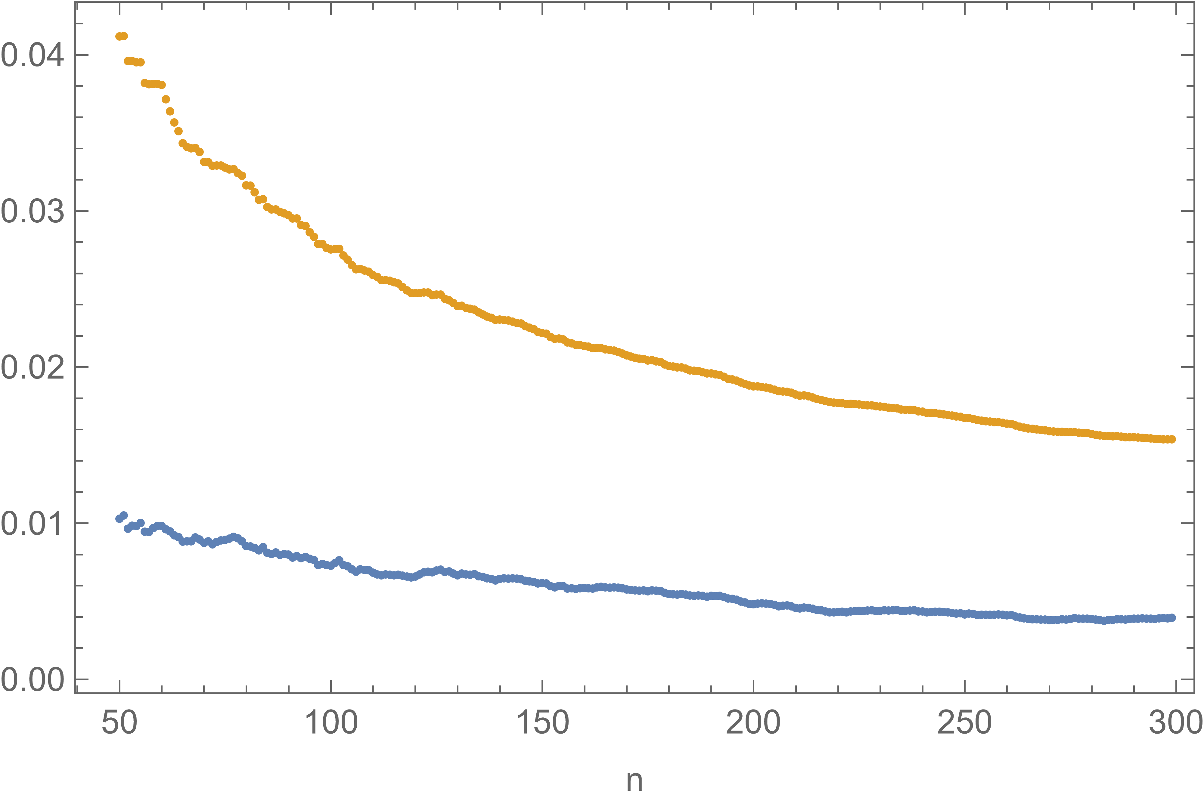
(a) Bernoulli data

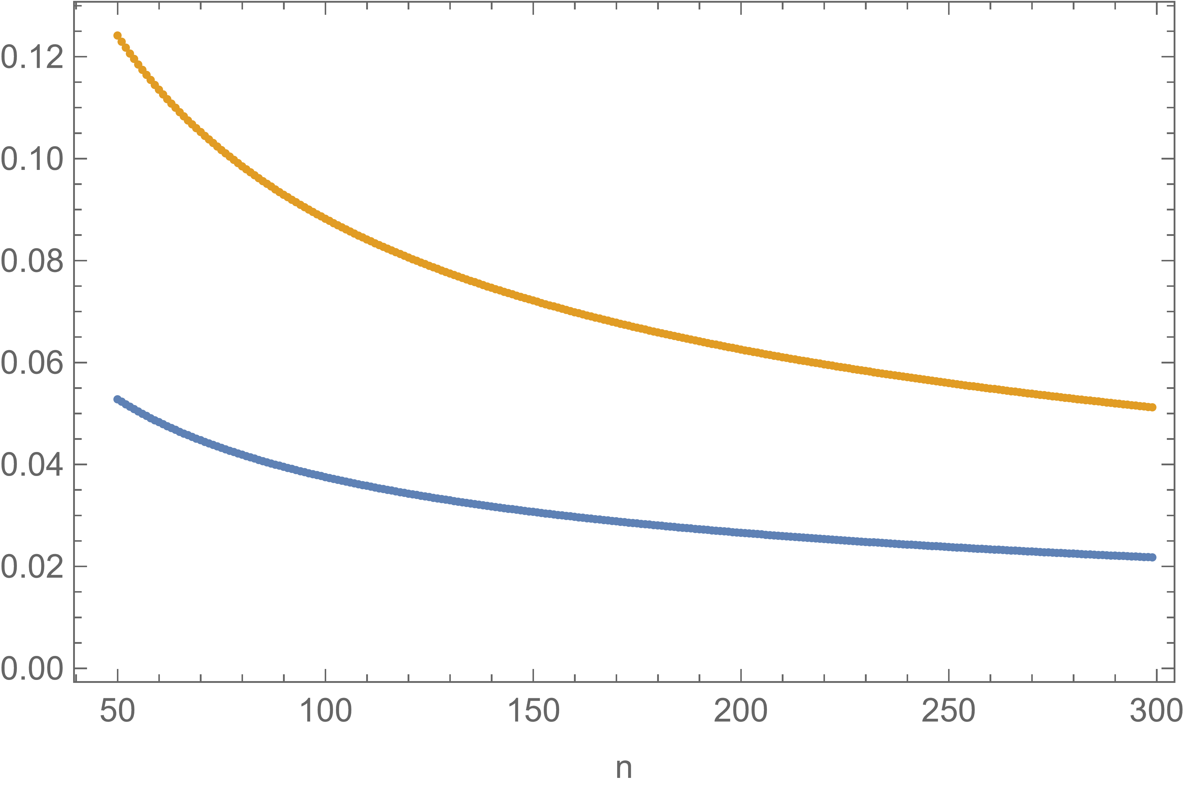
(b) Normal data

Figure 1: Numerical illustrations of our bounds for the normal approximation of the posterior standardised around the mode. Plotted are the true values of the total variation distance (evaluated through direct numerical integration) and the corresponding bounds for: Bernoulli data (Figure 1(a)), and normal data (Figure 1(b)). In each case we generated 5 samples of the corresponding probability distribution and took the average over these samples. The estimates and the bounds are computed over the same sample (with a sample size running from $50$ to $300$). More illustrations for some examples are provided in the Supplementary Material.

In each of the examples of this section, we provide total variation distance bounds for the normal approximation of the standardised posterior $\theta^{\star}$ (the standardisation based on the posterior mode). However, for a more efficient treatment, we only derive Wasserstein distance bounds, and bounds for the standardised posterior $\theta^{\dagger}$ (the standardisation based on the MLE) in select examples. These examples include the simple Example 1 for a Bernoulli likelihood with beta prior, and Examples 3 and 4 in which we obtain an exact formula for the Wasserstein distance between the standardised posterior $\theta^{\star}$ and the standard normal distribution. We remark that, in each example, only minor alterations are required to obtain bounds for $\theta^{\dagger}$. In Example 2, we demonstrate how the bounds of Section 2 involving the additional constant $\epsilon$ can result in simpler bounds. All bounds derived in this section are of the $O(n^{-1/2})$ rate (in the sense of Remark 1), as expected. In these examples it is easy to verify that the appropriate assumptions are satisfied; for conciseness we usually do not work through the details in the main text and defer a detailed description of the necessary computations to the Supplementary Material. Illustrations of the bounds over simulated samples are provided in Figure 1, and more illustrations are also provided in select examples in the Supplementary Material.

Before delving into the different examples, we recall the classical theory of moments of distributions from an exponential family. Let, for $t=(t_{1},\ldots,t_{k})$,

$$A(t)=\log\int_{\Theta}\exp\left(\theta^{\intercal}t-\lambda(\theta)\right)d\theta.$$

Setting now $t^{\star}=\big{(}\sum_{i=1}^{n}h_{i,1}(x_{i}),\ldots,\sum_{i=1}^{n}h_{i,k}(x_{i})\big{)}$ simple computation yield $\mathbb{E}[\theta_{i}]=\partial_{i}A(t^{\star})$, $i=1,\ldots,k$, and $\mathbb{E}[\theta_{i}\theta_{j}]=\partial_{i}\partial_{j}A(t^{\star})+\partial_{i}A(t^{\star})\partial_{j}A(t^{\star})$, $i,j=1,\ldots,k$, so that for all $k\times k$ matrices $H$ and all $\theta_{0}\in\Theta$ we have

$$\mathbb{E}[H(\theta-\theta_{0})] =H(\nabla A(t^{\star})-\theta_{0}),$$

$$\mathbb{E}[(H(\theta-\theta_{0}))(H(\theta-\theta_{0}))^{\intercal}] =H\left(\nabla^{2}A(t^{\star})+\nabla A(t^{\star})\nabla A(t^{\star})^{\intercal}-2\theta_{0}\nabla A(t^{\star})^{\intercal}+\theta_{0}\theta_{0}^{\intercal}\right)H^{\intercal}.$$

Example 1.

Consider i.i.d. Bernoulli data with parameter $p\in(0,1)$. This family of distributions can be written as an exponential family with natural parameter $\theta$ by taking

$$\theta=\log(p/(1-p)),\quad\Theta=(-\infty,\infty),\quad h(x)=x\mbox{ and }\beta(\theta)=\log(1+e^{\theta}).$$

We denote the prior $\pi_{0}(\theta)\propto\exp({-\eta(\theta)})$. We also write $\bar{x}=n^{-1}\sum_{i=1}^{n}x_{i}$.

We first study the normal approximation of the posterior distribution centred at its mode. We fix a conjugate prior on $\theta$, i.e. $\eta(\theta)=-\tau_{1}\theta+\tau_{2}\log(1+e^{\theta})$ for some $\tau_{1}>0$, $\tau_{2}-\tau_{1}>0$. Then

$$\tilde{\theta}=\log\left(\frac{\tau_{1}+n\bar{x}}{n(1-\bar{x})+\tau_{2}-\tau_{1}}\right).$$

Proposition 2 does not apply. Theorem 4 yields $d_{\mathrm{Wass}}(\theta^{\star},N)\leq\tilde{\Delta}_{n,\eta}(\mathbf{x})$ and $d_{\mathrm{TV}}(\theta^{\star},N)\leq\sqrt{\pi/8}\tilde{\Delta}_{n,\eta}(\mathbf{x})$ with

$$\tilde{\Delta}_{n,\eta}(\mathbf{x}) \leq\frac{1}{12\sqrt{3}}\frac{(n+\tau_{2})^{5/2}}{(\tau_{1}+n\bar{x})^{3/2}(n(1-\bar{x})+\tau_{2}-\tau_{1})^{3/2}}\mathbb{E}\left[(\theta^{\star})^{2}\right].$$

Using the exponential family structure we obtain an explicit formula for $\mathbb{E}[(\theta^{\star})^{2}]$ in terms of the parameters of the model and derivatives of the digamma function. Using (17), we also obtain a lower bound of the same $O(n^{-1/2})$ order. We can conclude that there exist functions $a(n,\bar{x},\tau_{1},\tau_{2})$ and $A(n,\bar{x},\tau_{1},\tau_{2})$ (whose expressions are provided in the Supplementary Material) such that

$$a(n,\bar{x},\tau_{1},\tau_{2})\leq{\sqrt{\frac{(n\bar{x}+\tau_{1})(n(1-\bar{x})+(\tau_{2}-\tau_{1}))}{n+\tau_{2}}}}{d_{\mathrm{Wass}}(\theta^{\star},N)}\leq A(n,\bar{x},\tau_{1},\tau_{2}).$$

As shown in the Supplementary Material, these functions satisfy $\lim_{n\to\infty}A(n,t,\tau_{1},\tau_{2})=1/(12\sqrt{3}t(1-t))$ and $\lim_{n\to\infty}a(n,t,\tau_{1},\tau_{2})=|1-2t|/2$ for all $t\in(0,1)$; these last two functions coincide when $t=(3\pm\sqrt{3})/6$.

Next, we study the normal approximation of the posterior standardised around the MLE. Some simple arguments yield

$$\hat{\theta}=\log\left(\frac{\bar{x}}{1-\bar{x}}\right).$$

Theorem 6 gives $d_{\mathrm{Wass}}(\theta^{\dagger},N)\leq\hat{\hat{\Delta}}_{\beta,\eta}(\mathbf{x})$ and $d_{\mathrm{TV}}(\theta^{\dagger},N)\leq\sqrt{\pi/8}\hat{\hat{\Delta}}_{\beta,\eta}(\mathbf{x})$ with

$$\hat{\hat{\Delta}}_{\beta,\eta}(\mathbf{x})\leq\frac{1}{\sqrt{n\bar{x}(1-\bar{x})}}\bigg{(}\frac{1}{12\sqrt{3}}\frac{1}{\bar{x}(1-\bar{x})}\mathbb{E}\left[(\theta^{\dagger})^{2}\right]+\|\eta^{\prime}\|_{\infty}\bigg{)}$$

with $\mathbb{E}[(\theta^{\dagger})^{2}]$, similarly as above, available in closed-form. In the case of the conjugate prior with exponent $\eta(\theta)=-\tau_{1}+\tau_{2}\log(1+e^{\theta})$, the necessary assumptions are satisfied and we have $\eta^{\prime}(\theta)=-\tau_{1}+\tau_{2}e^{\theta}/(1+e^{\theta})$, so that $\|\eta^{\prime}\|_{\infty}\leq\mathrm{max}\{\tau_{1},\tau_{2}-\tau_{1}\}$. For example, with an improper hyperbolic prior $\pi_{0}(\theta)=\cosh(\theta)=\frac{1}{2}(e^{\theta}+e^{-\theta})$ we have $\eta(\theta)=-\log(\cosh(\theta))$ with derivative $\eta^{\prime}(\theta)=-\tanh(\theta)$, which satisfies $\|\eta^{\prime}\|_{\infty}=1$.

Example 2.

Consider i.i.d. Poisson data with parameter $\mu>0$. This family of distributions can be written as an exponential family with natural parameter $\theta$ by taking

$$\theta=\log\mu,\quad\Theta=(-\infty,\infty),\quad h(x)=x\mbox{ and }\beta(\theta)=e^{\theta}.$$

We consider a conjugate gamma prior on $\mu$ of the form $\pi_{0}(\theta)\propto\exp({-\eta(\theta)})$ with $\eta(\theta)=-\tau_{1}\theta+\tau_{2}e^{\theta}$ for $\tau_{1},\tau_{2}>0$. Then

$$\tilde{\theta}=\log\left(\frac{\tau_{1}+n\bar{x}}{n+\tau_{2}}\right).$$

Proposition 2 applies and we obtain

$$d_{\mathrm{Wass}}(\theta^{\star},N)=\sqrt{n\bar{x}+\tau_{1}}\left(\log(n+\bar{x}+\tau_{1})-\psi(n+\bar{x}+\tau_{1})\right)\approx\frac{1}{\sqrt{4n\bar{x}+\tau_{1}}}.$$

For a total variation distance bound we can either work through inequality (15) (bound not reported here, see Supplementary Material) or through inequality (16) together with Markov’s inequality to get

$$d_{\mathrm{TV}}(\theta^{\star},N) \leq\frac{1}{2}\bigg{(}\frac{3+\sqrt{5}}{2}+e\bigg{)}\frac{\sqrt{\mathbb{E}[(\theta^{\star})^{2}]}}{\sqrt{\tau_{1}+n\bar{x}}}.$$

As in Example 1, we can obtain the moments of the posterior mode, which lead to

$$\mathbb{E}[(\theta^{\star})^{2}] \leq 1+\frac{1}{n\bar{x}+\tau_{1}}.$$

Example 3.

Consider i.i.d. normal data with known mean $m$ and unknown variance $\sigma^{2}$. This family of distributions can be written as an exponential family with natural parameter $\theta$ by taking

$$\theta=\sigma^{-2},\quad\Theta=(0,\infty),\quad h(x)=-(x-m)^{2}/2\mbox{ and }\beta(\theta)=-(1/2)\log\theta.$$

We consider a conjugate gamma prior on $\theta$ of the form $\pi_{0}(\theta)\propto\exp({-\eta(\theta)})$, where $\eta(\theta)=\tau_{1}\theta-\tau_{2}\log\theta$ for $\tau_{1}>0$ and $\tau_{2}>-1$. The posterior distribution $\theta$ has a gamma distribution with shape parameter $n/2+\tau_{2}+1$, and so Assumption 0 is satisfied if $n+2\tau_{2}>0$. Then

$$\tilde{\theta}=\frac{n+2\tau_{2}}{n\tilde{s}^{2}+2\tau_{1}},$$

where we let $n\tilde{s}^{2}=\sum_{i=1}^{n}(x_{i}-m)^{2}$. Applying inequality (15) yields

$$d_{\mathrm{TV}}(\theta^{\star},N) \leq\frac{\sqrt{\pi}}{2}\frac{1}{\sqrt{n+2\tau_{2}}}.$$

Similarly, inequalities (14) and (17) yield to identical upper and lower bounds for the Wasserstein distance, whence

$$d_{\mathrm{Wass}}(\theta^{\star},N)=\frac{\sqrt{2}}{\sqrt{n+2\tau_{2}}}.$$ (25)

Total variation and Wasserstein bounds for standardisation via the MLE are provided in the Supplementary Material.

Remark 10.

From equality (25) we deduce an exact formula for the Wasserstein distance between the gamma and normal distributions. Let $X\sim\Gamma(\alpha,\beta)$ with density $p(w)=\beta^{\alpha}w^{\alpha-1}e^{-\beta w}/\Gamma(\alpha)$, $w>0$, with $\alpha>1$ and $\beta>0$, and let $Y\sim N((\alpha-1)/\beta,(\alpha-1)/\beta^{2})$. Then

$$d_{\mathrm{Wass}}(X,Y)=\beta^{-1}.$$

In interpreting this formula, we note that $\mathrm{Mode}(X)=\mathrm{Mode}(Y)=(\alpha-1)/\beta$ and $\mathbb{E}[X]/\mathrm{Var}(X)=\mathbb{E}[Y]/\mathrm{Var}(Y)=\beta$.

Example 4.

Consider i.i.d.  Weibull data with density on the positive real line

$$p_{1}(x|\ell,m) =\frac{m}{\ell^{m}}x^{m-1}\mathrm{exp}\left\{-(x/\ell)^{m}\right\}=\mathrm{exp}\left\{-x^{m}{\ell^{-m}}+m\log x-\log x+\log m+\log(\ell^{-m})\right\}.$$

We suppose $m$ is known, and $\ell$ is the parameter of interest. Fix, for $\tau_{1}>0$ and $\tau_{2}>-1$, a (conjugate) gamma prior on $\theta=\ell^{-m}$ of the form $\pi_{0}(\theta)\propto e^{-\eta(\theta)}$, with $\eta(\theta)=\tau_{1}\theta-\tau_{2}\log\theta$ (for $\tau_{1}=0$ and $\tau_{2}=-1$ one obtains the improper Jeffreys prior for which our bounds also hold for $n\geq 2$). Therefore $\lambda(\theta)=\tau_{1}\theta-(\tau_{2}+n)\log\theta$ and we take $\Theta=(0,\infty)$. By the same reasoning as for the previous example, Assumption 0 holds if $n+\tau_{2}>0$. The situation is very similar to the previous example, so $\tilde{\theta}=(n+\tau_{2})/(\sum_{i}x_{i}^{m}+\tau_{1})$, and the same kind of bounds readily apply, namely, in the case of the standardisation by the posterior mode,

$$d_{\mathrm{TV}}(\theta^{\star},N)\leq\frac{\sqrt{2\pi}}{4}\frac{1}{\sqrt{n+\tau_{2}}},\quad d_{\mathrm{Wass}}(\theta^{\star},N)=\frac{1}{\sqrt{n+\tau_{2}}}.$$

This setting is also considered in [26, Example 5.2] where a Wasserstein bound is obtained from their general approach; their result is of course not competitive with ours (since we achieve equality).

Example 5.

Consider i.i.d.  negative binomial data with density

$$p_{1}(x|r,p) =\binom{x+r-1}{x}(1-p)^{r}p^{x}=\mathrm{exp}\left\{x\log p+\log\binom{x+r-1}{x}+r\log(1-p)\right\}.$$

We suppose $r$ is known, and $p$ is the parameter of interest. Then $h(x)=x$, $g(x)=\log\binom{x+r-1}{x}$ and the natural parameter is $\theta=\log p$; we take $\Theta=(-\infty,0)$ Fix, for $\tau_{1}>0$ and $\tau_{2}>-1$, a (conjugate) prior on $\theta$ of the form $\pi_{0}(\theta)\propto\exp(-\eta(\theta))$, where $\eta(\theta)=-{\theta\tau_{1}}-\tau_{2}\log(1-e^{\theta})$. Then (16) together with Markov’s inequality gives

$$d_{\mathrm{TV}}(\theta^{\star},N) \leq\frac{\sqrt{nr+\tau_{2}}\mathbb{E}[|\theta^{\star}|]}{2\sqrt{(n\bar{x}+\tau_{1})(nr+n\bar{x}+\tau_{1}+\tau_{2})}}\bigg{\{}2(3+\sqrt{5})\bigg{(}\log\bigg{(}\frac{n\bar{x}+\tau_{1}+\tau_{2}+nr}{n\bar{x}+\tau_{1}}\bigg{)}\bigg{)}^{-1}$$

$$\quad+\frac{(nr+\tau_{2})^{2}((n\bar{x}+\tau_{1}+\tau_{2}+nr)^{3}-(n\bar{x}+\tau_{1})^{3})}{(n\bar{x}+\tau_{1})^{3/2}(n\bar{x}+\tau_{1}+\tau_{2}+nr)^{3/2}(\sqrt{n\bar{x}+\tau_{1}+\tau_{2}+nr}-\sqrt{n\bar{x}+\tau_{1}})^{4}}\bigg{\}}.$$

where an explicit bound for $\mathbb{E}[|\theta^{*}|]$ is given in the Supplementary Material.

Example 6.

Consider i.i.d. multinomial data with parameters $(p_{1},\ldots,p_{k})^{\intercal}$ and individual likelihood

$$p_{1}(x|p)=\prod_{j=1}^{k}p_{j}^{x_{j}}=\mathrm{exp}\Bigg{\{}\sum_{j=1}^{k}x_{j}\log(p_{j})\Bigg{\}},$$ (26)

where $0<p_{1},\ldots,p_{k}<1$ with $\sum_{j=1}^{k}p_{j}=1$, and $x_{1},\ldots,x_{k}\in\{0,1\}$ with $\sum_{j=1}^{k}x_{j}=1$. We express the likelihood (26) as an exponential family by writing

$$p_{1}(x|p) =\mathrm{exp}\Bigg{\{}\sum_{j=1}^{k-1}x_{j}\log(p_{j})+\Bigg{(}1-\sum_{j=1}^{k-1}x_{j}\Bigg{)}\log(p_{k})\Bigg{\}}=\mathrm{exp}\Bigg{\{}\sum_{j=1}^{k-1}x_{j}\log\left(\frac{p_{j}}{p_{k}}\right)+\log(p_{k})\Bigg{\}},$$

so $h_{j}(x_{j})=x_{j}$, $g(x)=0$ and the natural parameter is $\theta=(\theta_{1},\ldots,\theta_{k-1})^{\intercal}$, where $\theta_{j}=\log(p_{j}/p_{k})$, $j=1,\ldots,k-1$, and $\Theta=\mathbb{R}^{k-1}$. Expressing the density in terms of $\theta$, we get $p_{j}(\theta)=p_{k}e^{\theta_{j}}$. Also, since $\sum_{j=1}^{k}p_{j}=1$, we obtain that $p_{k}+p_{k}\sum_{j=1}^{k-1}e^{\theta_{j}}=1$, so that $p_{k}=(1+\sum_{j=1}^{k-1}e^{\theta_{j}})^{-1}$. Thus, $\beta(\theta)=-\log(p_{k}(\theta))=\log(1+\sum_{j=1}^{k-1}e^{\theta_{j}}).$ Fix a (conjugate) Dirichlet prior on $p=(p_{1},\ldots,p_{k-1})^{\intercal}$ of the form $\pi_{0}(p)\propto p_{k}^{\tau_{k}-\sum_{j=1}^{k-1}\tau_{j}}\prod_{j=1}^{k-1}p_{j}^{\tau_{j}}$ for $\tau_{1},\ldots,\tau_{k-1}>-1$ and $\tau_{k}>\sum_{j=1}^{k-1}\tau_{j}-1$, so that $\pi_{0}(\theta)\propto e^{-\eta(\theta)}$, where $\eta(\theta)=-\sum_{j=1}^{k-1}\tau_{j}\theta_{j}+\tau_{k}\log(1+\sum_{j=1}^{k-1}e^{\theta_{j}}).$ Applying Theorem 1 yields, after some heavy computations, the bounds

$$d_{\mathrm{TV}}(\theta^{\star},N) \leq\frac{2\sqrt{2\pi}}{3}(k-1)^{2}\|C_{k}\|_{\infty}^{3}\frac{(n+\tau_{k})}{n^{3/2}}\sum_{u=1}^{k-1}\mathbb{E}[(\theta_{u}^{\star})^{2}],$$

$$d_{\mathrm{Wass}}(\theta^{\star},N) \leq(k-1)^{2}\|C_{k}\|_{\infty}^{3}\frac{(n+\tau_{k})}{n^{3/2}}\sum_{u=1}^{k-1}\mathbb{E}[(\theta_{u}^{\star})^{2}],$$

where the quantities $C_{k}$ are provided in the Supplementary Material, alongside formulas for the moments $\sum_{u=1}^{k-1}\mathbb{E}[(\theta_{u}^{\star})^{2}]$ in terms of the digamma function and the parameters of the model.

Example 7.

Consider i.i.d.  normal data with mean $\mu$ and variance $\sigma^{2}$, and thus density

$$p_{1}(x\,|\,\mu,\sigma^{2})=\mathrm{exp}\bigg{\{}-\frac{1}{2}\log(2\pi\sigma^{2})-\frac{\mu^{2}}{2\sigma^{2}}+\frac{x\mu}{\sigma^{2}}-\frac{x^{2}}{2\sigma^{2}}\bigg{\}}.$$

Then $\beta(\theta)=1/2\log(2\pi/\theta_{2})+\theta_{1}^{2}/(2\theta_{2})$, $g(x)=0$, $h_{1}(x)=x$, $h_{2}(x)=-x^{2}/2$ and the natural parameter is $\theta=(\theta_{1},\theta_{2})^{\intercal}=(\mu/\sigma^{2},1/\sigma^{2})^{\intercal}$, which lives on $\mathbb{R}\times(0,\infty)$. Fix, for $\tau_{1},\tau_{2},\tau_{3},\tau_{4}\in\mathbb{R}$ with $\tau_{4}>0,\tau_{1}<3/2,4\tau_{4}\tau_{2}>\tau_{3}^{2}$, a (conjugate) prior on $\theta$ of the form $\pi_{0}(\theta)\propto\exp({-\eta(\theta)})$, where $\eta(\theta)={\log(2\pi/\theta_{2})\tau_{1}+\theta_{1}^{2}\tau_{2}/\theta_{2}-\theta_{1}\tau_{3}+\theta_{2}\tau_{4}}$. The posterior mode is given by

$$\tilde{\theta}_{1}=\frac{(n+2\tau_{1})(\sum_{i}x_{i}+\tau_{3})}{(n+2\tau_{2})(\sum_{i}x_{i}^{2}+2\tau_{4})-(\sum_{i}x_{i}+\tau_{3})^{2}},\quad\tilde{\theta}_{2}=\frac{(n+2\tau_{1})(n+2\tau_{2})}{(n+2\tau_{2})(\sum_{i}x_{i}^{2}+2\tau_{4})-(\sum_{i}x_{i}+\tau_{3})^{2}}.$$

Using inequality (9) together with $r=1$ yields, after relatively heavy computations provided in the Supplementary Material,

$$d_{\mathrm{TV}}(\theta^{\star},N) \leq\frac{64\sqrt{\pi}}{3\lambda_{\mathrm{min}}^{3/2}}(n+2(\tau_{1}+\tau_{2}))\bigg{(}1+\frac{7}{2}\tilde{\theta}_{1}^{2}+\frac{5}{8}\tilde{\theta}_{2}^{2}\bigg{)}\bigg{(}\frac{1}{\tilde{\theta}_{2}^{2}}+\frac{4}{\tilde{\theta}_{2}^{4}}\bigg{)}\big{(}\mathbb{E}[(\theta_{1}^{\star})^{2}]+\mathbb{E}[(\theta_{2}^{\star})^{2}]\big{)}$$

$$\quad+\frac{3+\sqrt{5}}{\tilde{\theta}_{2}(\lambda_{\mathrm{min}})^{1/2}}\left(\mathbb{E}[|\theta_{1}^{\star}|]+\mathbb{E}[|\theta_{2}^{\star}|]\right),$$

where $\lambda_{\mathrm{min}}$ is the smallest eigenvalue of $\mathbf{H}_{\lambda}(\tilde{\theta})$; the expression is given in the Supplementary Material. The various expectations can be tackled using the same tools as in the previous examples yielding to explicit quantities depending on the model’s parameters, and $\lambda_{\mathrm{min}}=O(n)$ so that we have in total the optimal $O(n^{-1/2})$ rate.

Example 8.

Consider the standard linear regression model with unknown variance ,i.e.

$$X=M\xi+\epsilon,$$

where $M\in\mathbb{R}^{n\times k}$ is the design matrix, $\xi\in\mathbb{R}^{k}$ and $\epsilon\sim N(0,I_{n}\sigma^{2})$. The density of $X_{i}$ is given by

$$p_{1,i}(x)=\frac{1}{\sqrt{2\pi\sigma^{2}}}\exp\bigg{(}-\frac{1}{2\sigma^{2}}(x-\vec{m}_{i}\xi)^{2}\bigg{)},$$

where $\vec{m}_{i}$ denotes the $i$th row of the matrix $M$. The natural parameter is $\theta=(\xi_{1}/\sigma^{2},\ldots,\xi_{k}/\sigma^{2},1/\sigma^{2})\in\mathbb{R}^{k}\times(0,\infty)$. Moreover, we have for $i=1,\ldots,n$ the functions $h_{i,j}(x)=m_{i,j}x$, $j=1,\ldots,k$, $h_{i,k+1}(x)=-x^{2}/2$ and $\beta_{i}(\theta)=-1/2\log(\theta_{k+1})+\frac{1}{2\theta_{k+1}}(\vec{m}_{i}\vec{\theta})^{2}$, where $\vec{\theta}=(\theta_{1},\ldots,\theta_{k})$. We choose a conjugate prior of the form

$$\eta(\theta)=\tau_{0}\log(\theta_{k+1})+\vec{\tau}\vec{\theta}+\tau_{k+1}\theta_{k+1}+\frac{1}{2\theta_{k+1}}\vec{\theta}^{\,\intercal}\tau\vec{\theta},$$

where $\tau_{0}>-1$, $\tau_{k+1}>0$, $\tau=\tau_{i,j}$, $1\leq i,j\leq k$ is a symmetric positive definite matrix and $\vec{\tau}=(\tau_{1},\ldots,\tau_{k})\in\mathbb{R}^{k}$ with $\tau_{k+1}-\vec{\tau}^{\,\intercal}\tau^{-1}\vec{\tau}/2<0$. We center around the MLE given by

$$\hat{\theta}=\frac{(n(M^{\intercal}M)^{-1}M^{\intercal}X,n)}{X^{\intercal}X-X^{\intercal}M(M^{\intercal}M)^{-1}M^{\intercal}X}\in\mathbb{R}^{k+1}.$$

We apply the conditioned version of the first part of Theorem 5 to get, after heavy computations provided in the Supplementary Material,

$$d_{\mathrm{TV}}(\theta^{\dagger},N)\leq \frac{(k+1)^{7/2}}{12(\lambda_{\mathrm{min}})^{3/2}}\bigg{(}\frac{1}{\hat{\theta}_{k+1}^{2}}+\frac{4}{\hat{\theta}_{k+1}^{4}}\bigg{)}\bigg{(}24(2\tau_{0}+n)+6\kappa k\hat{\theta}_{k+1}+\kappa\big{(}48+k\hat{\theta}_{k+1}^{2}\big{)}\bigg{)}\sum_{u=1}^{k+1}\mathbb{E}\big{[}(\theta^{\dagger}_{u})^{2}\big{]}$$

$$+\frac{3+\sqrt{5}}{\hat{\theta}_{k+1}\sqrt{\lambda_{\mathrm{min}}}}\sum_{i=1}^{k+1}\mathbb{E}[|\theta_{i}^{\dagger}|]+\frac{1}{\sqrt{\lambda_{\mathrm{min}}}}\sum_{l=1}^{k+1}|\partial_{l}\eta(\hat{\theta})|+\frac{1}{\sqrt{\lambda_{\mathrm{min}}}}\sum_{u=1}^{k+1}\sum_{l=1}^{k+1}\sum_{m=1}^{k+1}|c_{l,m}b_{m,u}|\mathbb{E}[|\theta_{u}^{\dagger}|],$$

where $\kappa=\|M+\tau\|_{\infty}$, with $\|\cdot\|_{\infty}$ the absolute row sum norm, $\lambda_{\min}$ a quantity similar to what was obtained in the previous example, and $c_{l,m},b_{l,m}$ are defined by equation (19). In the Supplementary Material, we express all these quantities, including the various moments of the standardised posterior, in terms of the parameters of the model.

4 Proofs of main results

4.1 About Stein’s method of comparison of operators

As announced in the Introduction, we achieve all our general bounds through comparison of Stein operators. The idea behind Stein’s method can be sketched as follows. As developed in [41], for a standard normal target, the method starts by acknowledging the following two facts: (i) a random variable $Z$ is standard normal ${N}(0,1)$ if and only if for all sufficiently regular smooth functions $f$ it holds that $\mathbb{E}[f^{\prime\prime}(Z)]=\mathbb{E}[Zf^{\prime}(Z)]$, and (ii) for any suitable (for example, Lipschitz) test function $h:\mathbb{R}\rightarrow\mathbb{R}$ there is a sufficiently regular smooth function $f=f_{h}$ solving the Stein equation $f^{\prime\prime}(w)-wf^{\prime}(w)=h(w)-\mathbb{E}[h(Z)]$. In [41], Stein combined these two facts to deduce that for any random variable of interest $W$ and any suitable test function $h$, we have $\mathbb{E}[h(W)]-\mathbb{E}[h(Z)]=\mathbb{E}[f_{h}^{\prime\prime}(W)-Wf^{\prime}_{h}(W)]$, the right-hand-side being the starting point for performing approximation in law of $W$ by $Z$. One of the reasons for which this identity has turned out so useful is the fact that the left-hand side in the last expression generates an integral probability metric and is thus a relevant probabilistic discrepancy, while the right-hand side depends only and explicitly on the distribution of $W$, the standard normal distribution being encoded by the operator $T_{Z}f(w)=f^{\prime\prime}(w)-wf^{\prime}(w)$, and is therefore amenable to computations and manipulations. A similar approach can be set up for many distributions simply by changing the operator; for a random vector $W$ on $\mathbb{R}^{k}$ with density $p$ a Stein density operator (sometimes also called Langevin-Stein operator, see [1]) is given by

$$T_{W}f(w)=\Delta f(w)+\langle\nabla\log p(w),\nabla f(w)\rangle$$ (27)

with $\Delta$ the Laplacian and $\langle\cdot,\cdot\rangle$ the scalar product (see formula (22) of [32]). If $W\sim p$, then $\mathbb{E}[T_{W}f(W)]=0$ for a large class of functions $f$; the collection of all real-valued functions $f$ for which $\mathbb{E}[T_{W}f(W)]=0$ is called the Stein class of $T_{W}$. Moreover, for $N\sim N(0,I_{k})$, the $k$-dimensional standard multivariate normal distribution with mean vector 0 and covariance matrix $I_{k}$, the $k\times k$ identity matrix, we have

$$T_{N}f(w)=\Delta f(w)-\langle w,\nabla f(w)\rangle;$$ (28)

this operator was first obtained by [4, 21] in their development of Stein’s method for multivariate normal approximation. One can then assess the distance to the $N(0,I_{k})$ distribution with respect to an integral probability metric $d_{\mathcal{H}}$, where $\mathcal{H}$ is some measure determining class of functions, by taking

$$d_{\mathcal{H}}(W,N):=\sup_{h\in\mathcal{H}}|\mathbb{E}[h(W)]-\mathbb{E}[h(N)]|=\sup_{f_{h}}|\mathbb{E}[T_{N}f_{h}(W)-T_{W}f_{h}(W)]|,$$ (29)

where the final supremum is taken over all solutions $f_{h}$ with $h\in\mathcal{H}$ to the $N(0,I_{k})$ Stein equation $T_{N}f(w)=h(w)-\mathbb{E}[h(N)]$, as long as these $f_{h}$’s are in the Stein class of $T_{W}$.

The comparison of Stein operators proves fruitful for our purpose of obtaining quantitative normal approximations for the posterior for several reasons. Firstly, a tractable Stein density operator is available for exponential family distributions (see Lemma 3 in Section 4.3). Crucially, normalising constants are irrelevant in the Stein density operator, and we have the neat decomposition $\log p_{2}=\log\pi_{0}+\sum_{i=1}^{n}\log p_{1,i}+C$, where $\pi_{0}$ is the prior distribution, $p_{1,i}$ are the likelihoods of the observations and the contribution $C$, which comes from the normalising constant, vanishes under differentiation. Moreover, as can be seen from the right-hand side of (29), the second-order partial derivatives of the solution of the multivariate normal Stein equation cancel, and we are only left with first-order partial derivatives. These first-order derivatives are more regular, and so we are able to obtain optimal order $n^{-1/2}$ bounds in the often technically demanding to work with total variation distance, even in the multivariate setting.

4.2 About the solutions to the standard normal Stein equation

Central to Stein’s method for normal approximation [4, 21] is the so-called Stein equation for the standard $k$-dimensional normal distribution:

$$\Delta f(w)-\langle w,\nabla f(w)\rangle=h(w)-\mathbb{E}[h(N)],$$ (30)

where $N\sim N(0,I_{k})$ and $h:\mathbb{R}^{k}\rightarrow\mathbb{R}$ is a suitable test function. We recall some useful facts concerning the solutions to (30), according to whether $h\in\mathcal{H}_{\mathrm{Wass}}$ (this will be necessary for the bounds in Wasserstein distance), $h\in\mathcal{H}_{\mathrm{TV}}$ (for the bounds in total variation distance), or $h\in C_{P}^{1}(\mathbb{R}^{k})$ (for Theorem 3 and inequality (5)).

Bounds in the multivariate setting

We first consider the multivariate setting $k\geq 1$. If $h\in\mathcal{H}_{\mathrm{Wass}}$ (i.e. if $h$ is Lipschitz with constant 1), then the function

$$f_{h}(w)=-\int_{0}^{1}\frac{1}{2s}\left\{\mathbb{E}[h(s^{1/2}w+(1-s)^{1/2}N)]-\mathbb{E}[h(N)]\right\}\,ds$$ (31)

is a solution to (30) (see [16, Proposition 2.1]). Moreover, we have the bound

$$|f_{h}|_{1}\leq|h|_{1}\leq 1,$$ (32)

where $|f|_{1}:=\max_{1\leq j\leq k}\|\partial_{j}f(w)\|_{\infty}$. This bound was proved under the stronger assumption that $h$ is thrice differentiable by [20], although examining their proof, together with the result of [16, Proposition 2.1], shows that the assumption $h\in\mathcal{H}_{\mathrm{Wass}}$ suffices.

Next, consider $h\in\mathcal{H}_{\mathrm{T}V}$, that is, $h(\cdot)=\mathbb{I}[\cdot\in A]$ with $A\subset\mathcal{B}(\mathbb{R}^{k})$. Solutions to (30) being only valid for points $w\in\mathbb{R}^{k}$ where $h(w)$ is locally Hölder continuous (see [21, p. 726]), we cannot directly work with the Stein equation (30) with such indicator test functions. We work around this difficulty by applying the smoothing approach used by [21]. We consider the smoothed indicator functions $h_{t}(w)=\int_{\mathbb{R}^{k}}h(t^{1/2}y+(1-t)^{1/2}w)\,\phi(y)\,dy$, where $0<t<1$, $h\in\mathcal{H}_{\mathrm{T}V}$ and $\phi(y)$ is the probability density function of $N\sim N(0,I_{k})$. Observe that $\mathbb{E}[h_{t}(N)]=\mathbb{E}[h(N)]$ for all $t$, as noted by [36]. Then the functions

$$\psi_{t}(w):=-\int_{t}^{1}\frac{1}{2(1-s)}\{h_{s}(w)-\mathbb{E}[h(N)]\}\,ds$$ (33)

are well-defined solutions of

$$\Delta\psi_{t}(w)-\langle w,\nabla\psi_{t}(w)\rangle=h_{t}(w)-\mathbb{E}[h_{t}(N)]$$ (34)

for all $x\in\mathbb{R}^{k}$ and all $0<t<1$. Bounds for the derivatives of $\psi_{t}(w)$ were given by [21, Lemma 2.1] up to a universal constant. In the following lemma, we provide explicit constants for a bound on the first-order partial derivatives that will be needed in the sequel. The proof is given in Appendix A.

Lemma 1.

Let $h:\mathbb{R}^{k}\rightarrow\mathbb{R}$ be a bounded measurable function. Then, for $0<t<1$,

$$|\psi_{t}|_{1}\leq\sqrt{\frac{\pi}{2}}\|h-\mathbb{E}[h(N)]\|_{\infty}.$$ (35)

We remark that the upper bound in (35) is independent of $t$; this property is not enjoyed by higher order derivatives of $\psi_{t}$ (see [21, Lemma 2.1]). To account for the error introduced by smoothing $h$, we shall make use of the following specialisation of Lemma 2.11 of [21], which was derived using standard smoothing inequalities (see [5, Lemma 11.14]); a similar version of the smoothing lemma of [21] is given in [36].

Lemma 2 (Götze [21], Lemma 2.11).

Let $W$ be a $k$-dimensional random vector. Let $0<t<1$. Then

$$d_{\mathrm{TV}}(W,N)\leq\frac{4}{3}\sup_{h\in\mathcal{H}_{\mathrm{TV}}}|\mathbb{E}[h_{t}(W)]-\mathbb{E}[h_{t}(N)]|+\frac{5}{2}\frac{a_{k}\sqrt{t}}{1-t},$$

where $a_{k}^{2}$ is the $7/8$-quantile of the chi-square distribution with $k$ degrees of freedom.

Finally, suppose that $h\in C_{P}^{1}(\mathbb{R}^{k})$, where $P(w)=A+\sum_{i=1}^{k}B_{i}|w_{i}|^{r_{i}}$, for $A\geq 0$, $B_{1},\ldots,B_{k}\geq 0$ and $r_{1},\ldots,r_{k}\geq 0$. Then, we have the following non-uniform bound (given in [19], improving on a bound of [18]): for $j=1,\ldots,k$ and $w\in\mathbb{R}^{k}$,

$$|\partial_{j}f_{h}(w)|\leq A+\sum_{i=1}^{k}2^{r_{i}/2}B_{i}\left(|w_{i}|^{r_{i}}+\mu_{r_{i}}\right),$$ (36)

where $\mu_{r}$ denotes the $r$-th absolute moment of the standard normal distribution.

Bounds in the univariate case

We now turn to the univariate case ($k=1$). The Stein equation (30) reduces to the standard normal Stein equation of [41]:

$$f^{\prime\prime}(w)-wf^{\prime}(w)=h(w)-\mathbb{E}[h(N)],$$ (37)

where $N$ now denotes a standard normal random variable. We are not aware of bounds for $\|f_{h}^{\prime}\|_{\infty}$ that improve on (32) for Lipschitz test functions (see e.g. also [13, Proposition 3.13] or [28, Lemma 2.7]). Similarly, (36) is the best bound available for functions in $C_{P}^{1}(\mathbb{R})$. Improved univariate total variation distance bounds are obtained by taking advantage of special properties enjoyed by the solution of the standard normal Stein equation in this case. Let $A\subset\mathcal{B}(\mathbb{R})$, and suppose that $h(w)=\mathbb{I}[w\in A]$. For such a test function, the unique absolutely continuous bounded solution to the univariate Stein equation must satisfy

$$f^{\prime}_{h}(w)=e^{w^{2}/2}\int_{-\infty}^{w}\{h(s)-\mathbb{E}[h(N)]\}e^{-s^{2}/2}\,ds,$$ (38)

and satisfies the bound

$$|f^{\prime}_{h}(w)|\leq\mathrm{min}(\sqrt{\pi/8},1/|w|),\quad w\in\mathbb{R}$$ (39)

(see [14, Example 2.32] and [17, Lemma 2.5]).

4.3 Two preparatory lemmas

As mentioned above (see equation (29)), we prove our main results by Stein’s method of comparison of operators, comparing the standard $k$-dimensional multivariate normal Stein operator $T_{N}$ (see (28)) with well-chosen Stein operators for $\theta^{\star}$ and $\theta^{\dagger}$, respectively.

Lemma 3.

For $1\leq i,j\leq k$ we let $a_{i,j}=((\mathbf{H}_{\lambda}(\tilde{\theta}))^{-1/2})_{i,j}$ and $b_{i,j}=((\mathbf{H}_{\tilde{\beta}}(\hat{\theta}))^{-1/2})_{i,j}$. The Stein density operator (27) for $\theta^{\star}$ is

$$T_{\theta^{\star}}f(w)=\Delta f(w)+\sum_{j=1}^{k}\sum_{u=1}^{k}a_{j,u}\Bigg{(}\sum_{i=1}^{n}h_{u}(x_{i})-\partial_{u}\lambda\left(\big{(}\mathbf{H}_{\lambda}(\tilde{\theta})\big{)}^{-1/2}w+\tilde{\theta}\right)\Bigg{)}\partial_{j}f(w),$$ (40)

while for $\theta^{\dagger}$ it is

$$T_{\theta^{\dagger}}f(w)=\Delta f(w)+\frac{1}{\sqrt{n}}\sum_{j=1}^{k}\sum_{u=1}^{k}b_{j,u}\Bigg{(}\sum_{i=1}^{n}h_{u}(x_{i})-\partial_{u}\lambda\left(\big{(}\mathbf{H}_{\tilde{\beta}}(\hat{\theta})\big{)}^{-1/2}w+\hat{\theta}\right)\Bigg{)}\partial_{j}f(w).$$ (41)

Proof.

Both formulas follow from a direct computation. We prove (40); formula (41) is obtained through a similar argument. Letting $p^{\star}$ denote the density of $\theta^{\star}$, we clearly have

$$p^{\star}(w) =\big{(}\mathrm{det}(\mathbf{H}_{\lambda}(\tilde{\theta}))\big{)}^{-1/2}p_{2}\left(\big{(}\mathbf{H}_{\lambda}(\tilde{\theta})\big{)}^{-1/2}w+\tilde{\theta}\,\Big{|}\,\mathbf{x}\right)$$

$$\propto\exp\Bigg{\{}\sum_{j=1}^{k}\left(\left(\big{(}\mathbf{H}_{\lambda}(\tilde{\theta})\big{)}^{-1/2}w\right)_{j}+\tilde{\theta}_{j}\right)\sum_{i}h_{j}(x_{i})-\lambda\left(\big{(}\mathbf{H}_{\lambda}(\tilde{\theta})\big{)}^{-1/2}w+\tilde{\theta}\right)\Bigg{\}}.$$

Then

$$\partial_{j}\log p^{\star}(w)=\sum_{u=1}^{k}a_{j,u}\Bigg{(}\sum_{i=1}^{n}h_{u}(x_{i})-\partial_{u}\lambda\left(\big{(}\mathbf{H}_{\lambda}(\tilde{\theta})\big{)}^{-1/2}w+\tilde{\theta}\right)\Bigg{)},$$

so that the Stein density operator (27) reads as announced. ∎

Lemma 4.

Let $\mathcal{H}=\mathcal{H}_{\mathrm{Wass}}$, or $\mathcal{H}_{\mathrm{TV}}$ (when $k=1$). Then, for all $h\in\mathcal{H}$,

$$\mathbb{E}[T_{\theta^{\star}}f_{h}(\theta^{\star})]=\mathbb{E}[T_{\theta^{\dagger}}f_{h}(\theta^{\dagger})]=0,$$

for $f_{h}$ the solution to the Stein equation (30). The same conclusion holds for $h\in\mathcal{H}=C_{P}^{1}(\mathbb{R}^{k})$ with $P(w)=A+\sum_{m=1}^{k}B_{m}|w_{m}|^{r_{m}}$, under the additional assumption that $\mathbb{E}[|\theta^{\star}|^{r_{*}}]<\infty$ or $\mathbb{E}[|\theta^{\dagger}|^{r_{*}}]<\infty$, where $r_{*}=\mathrm{max}\{r_{1},\ldots,r_{k}\}$. Moreover, for $\psi_{t}$, $0<t<1$, defined as in (33), we have

$$\mathbb{E}[T_{\theta^{\star}}\psi_{t}(\theta^{\star})]=\mathbb{E}[T_{\theta^{\dagger}}\psi_{t}(\theta^{\dagger})]=0.$$

Proof.

We prove the lemma for $\theta^{\star}$; exactly the same proof applies for the standardised posterior $\theta^{\dagger}$. For $h\in\mathcal{H}$, to conclude that $\mathbb{E}[T_{\theta^{\star}}f_{h}(\theta^{\star})]=0$, we need to prove that $f_{h}$ is in the Stein class of $T_{\theta^{\star}}$. According to part (i) of Section 3.4.3 and Definition 3.6 of [16], it suffices to prove that for all $h\in\mathcal{H}$ the solution $f_{h}$ is (i) twice differentiable with $\partial_{i,j}f_{h}\in L^{1}(\theta^{\star})$ for all $1\leq i,j\leq k$ and (ii) $p^{\star}(\theta)\partial_{j}f_{h}(\theta)=0$ for all $\theta$ on the boundary of the support of $\theta^{\star}$. To conclude that $\mathbb{E}[T_{\theta^{\star}}\psi_{t}(\theta^{\star})]=0$ for $0<t<1$, we need to verify the same conditions with $f_{h}$ replaced by $\psi_{t}$.

For $\mathcal{H}=\mathcal{H}_{\mathrm{Wass}}$, or $\mathcal{H}_{\mathrm{TV}}$ (when $k=1$), it suffices to show that all second-order partial derivatives of $f_{h}$ exist and that the first- and second-order partial derivatives are bounded, as Assumption 0 ensures that the density of $\theta^{\star}$ vanishes at the boundary of the support. For $\mathcal{H}=\mathcal{H}_{\mathrm{Wass}}$ the conditions are satisfied because $f_{h}$ is twice differentiable [16, Proposition 2.1] and satisfies $|f_{h}|_{1}\leq 1$ (see (32)) and $|f_{h}|_{2}\leq\sqrt{2/\pi}$ (see [17, Proposition 2.1], where $|f|_{2}:=\mathrm{max}_{1\leq i,j\leq k}\|\partial_{i,j}f\|_{\infty}$. Similarly, for $h\in\mathcal{H}_{\mathrm{TV}}$ ($k=1$), $f_{h}$ is twice differentiable and satisfies $\|f_{h}^{\prime}\|_{\infty}\leq\sqrt{\pi/8}$ (see (39)) and $\|f_{h}^{\prime\prime}\|_{\infty}\leq 2$ (see [11, Lemma 2.4]). Also, for $0<t<1$, the solution $\psi_{t}$ (as given in (33)) is twice differentiable and satisfies $|\psi_{t}|_{1}\leq\sqrt{\pi/2}$ (see (35)) and $|\psi_{t}|_{2}\leq C\log(t^{-1})$ for some universal constant $C>0$ (see [21, Lemma 2.1]), as required. Finally, we suppose that $h\in C_{P}^{1}(\mathbb{R}^{k})$. Again, $f_{h}$ is twice differentiable with $|\partial_{j}f_{h}(w)|\leq A+\sum_{m=1}^{k}2^{r_{m}/2}B_{m}(|w_{m}|^{r_{i}}+\mu_{r_{m}})$ (see (36)) and $|\partial_{i,j}f_{h}(w)|\leq A+\sum_{m=1}^{k}2^{r_{m}/2}B_{m}(|w_{m}|^{r_{m}}+\mu_{r_{m}+1})$ for $w\in\mathbb{R}^{k}$ (see [19, Proposition 2.1]). Conditions (i) and (ii) can now be seen to be satisfied due to Assumption 0 and our assumption that $\mathbb{E}[|\theta^{\star}|^{r_{*}}]<\infty$. ∎

4.4 Proofs of the main results

Proof of Theorems 1 and 3.

Let $\mathcal{H}$ be a collection of real-valued functions such that $\mathbb{E}[T_{\theta^{\star}}f_{h}(\theta^{\star})]=0$ for all $h\in\mathcal{H}$, with $f_{h}$ the solution to the corresponding Stein equation (30). Then, for all $h\in\mathcal{H}$,

$$\mathbb{E}[h(\theta^{\star})]-\mathbb{E}[h(N)] =\mathbb{E}\left[T_{N}f_{h}(\theta^{\star})\right]=\mathbb{E}\left[T_{N}f_{h}(\theta^{\star})\right]-\mathbb{E}\left[T_{\theta^{\star}}f_{h}(\theta^{\star})\right]=\mathbb{E}\left[(T_{N}-T_{\theta^{\star}})f_{h}(\theta^{\star})\right]$$

$$:=-\mathbb{E}\left[\langle L(\theta^{\star},n,\mathbf{x})+\theta^{\star},\nabla f_{h}(\theta^{\star})\rangle\right],$$

where $L(w,n,\mathbf{x})=(L_{1}(w,n,\mathbf{x}),\ldots,L_{k}(w,n,\mathbf{x}))^{\intercal},$ with, for $j=1,\ldots,k$,

$$L_{j}(w,n,\mathbf{x}):=\sum_{l=1}^{k}a_{j,l}\left(\sum_{i=1}^{n}h_{i,l}(x_{i})-\partial_{l}\lambda\left(\big{(}\mathbf{H}_{\lambda}(\tilde{\theta})\big{)}^{-1/2}w+\tilde{\theta}\right)\right)$$

(the $a_{j,l}$’s are defined in the statement of Lemma 3). Now, we Taylor expand $L_{j}(w,n,\mathbf{x})$ around $w=0$. The following formulas will be useful:

$$\partial_{w_{u}}L_{j}(w,n,\mathbf{x}) =-\sum_{l=1}^{k}\sum_{m=1}^{k}a_{j,l}a_{u,m}\partial_{l,u}\lambda\left(\big{(}\mathbf{H}_{\lambda}(\tilde{\theta})\big{)}^{-1/2}w+\tilde{\theta}\right),$$

$$\partial_{w_{u},w_{v}}L_{j}(w,n,\mathbf{x}) =-\sum_{l=1}^{k}\sum_{m=1}^{k}\sum_{p=1}^{k}a_{j,l}a_{u,m}a_{v,p}\partial_{l,u,v}\lambda\left(\big{(}\mathbf{H}_{\lambda}(\tilde{\theta})\big{)}^{-1/2}w+\tilde{\theta}\right).$$

Using Fact 1a, we have that $L_{j}(0,n,\mathbf{x})=0$. In addition,

$$\partial_{w_{u}}L_{j}(0,n,\mathbf{x}) =-\sum_{l=1}^{k}\sum_{m=1}^{k}a_{j,l}a_{u,m}\partial_{l,u}\lambda(\tilde{\theta})$$

$$=-\big{(}(\mathbf{H}_{\lambda}(\tilde{\theta}))^{-1/2}\mathbf{H}_{\lambda}(\tilde{\theta})(\mathbf{H}_{\lambda}(\tilde{\theta}))^{-1/2}\big{)}_{j,u}=-(I_{k})_{j,u}=-\delta_{j,u},$$

where $\delta_{j,u}$ is the Kronecker delta. We now use a Taylor expansion with explicit remainder (compare with [15, p. 141]),

$$L_{j}(w,n,\mathbf{x})+w_{j}$$

$$=-\sum_{u=1}^{k}\sum_{v=1}^{k}w_{u}w_{v}\int_{0}^{1}\!\int_{0}^{1}y_{2}\sum_{l=1}^{k}\sum_{m=1}^{k}\sum_{p=1}^{k}a_{j,l}a_{u,m}a_{v,p}\partial_{l,u,v}\lambda\left(y_{1}y_{2}\big{(}\mathbf{H}_{\lambda}(\tilde{\theta})\big{)}^{-1/2}w+\tilde{\theta}\right)\,dy_{1}\,dy_{2}$$

$$=-\sum_{u=1}^{k}\sum_{v=1}^{k}w_{u}w_{v}\mathbb{E}\bigg{[}Y_{2}\sum_{l=1}^{k}\sum_{m=1}^{k}\sum_{p=1}^{k}a_{j,l}a_{u,m}a_{v,p}\partial_{l,u,v}\lambda\left(Y_{1}Y_{2}\big{(}\mathbf{H}_{\lambda}(\tilde{\theta})\big{)}^{-1/2}w+\tilde{\theta}\right)\bigg{]},$$

where $Y_{1},Y_{2}\sim U(0,1)$ are independent of each other and all other randomness involved. Then

$$\mathbb{E}[h(\theta^{\star})]-\mathbb{E}[h(N)] =\mathbb{E}\Bigg{[}\sum_{j=1}^{k}\sum_{u=1}^{k}\sum_{v=1}^{k}\theta_{u}^{\star}\theta_{v}^{\star}\mathbb{E}\bigg{[}Y_{2}\sum_{l=1}^{k}\sum_{m=1}^{k}\sum_{p=1}^{k}a_{j,l}a_{u,m}a_{v,p}\times$$

$$\quad\times\partial_{l,u,v}\lambda\left(Y_{1}Y_{2}\big{(}\mathbf{H}_{\lambda}(\tilde{\theta})\big{)}^{-1/2}\theta^{\star}+\tilde{\theta}\right)\,\Big{|}\,\theta^{\star}\bigg{]}\partial_{j}f_{h}(\theta^{\star})\Bigg{]},$$ (42)

which, after rearranging, leads to the functions $\tilde{\Upsilon}^{\lambda}_{l,u,v}(\cdot)$ ($1\leq l,u,v\leq k$) given in (5).

We now can already obtain the Wasserstein bound in (7) from Theorem 1 as well as the bound (11) from Theorem 3. For the first one, since $|f_{h}|_{1}\leq 1$ when $h\in\mathcal{H}_{\mathrm{Wass}}$ (recall (32)), simplifying using the triangle inequality and the formulas $R_{u}^{\lambda}=|\sum_{v=1}^{k}a_{u,v}|$ and $\tilde{R}_{u}^{\lambda}=\sum_{v=1}^{k}|a_{u,v}|$, $u=1,\ldots,k$, shows that the expression $\tilde{\Delta}_{\lambda}$ from (6) indeed bounds $\sup_{h\in\mathcal{H}_{\mathrm{Wass}}}|\mathbb{E}[h(\theta^{\star})]-\mathbb{E}[h(N)]|$ and thus the Wasserstein bound from (7) follows. Proceeding similarly, but using the bound (36) instead of the bound (32) yields inequality (11).

All that remains is to derive the total variation distance bound in (7) from Theorem 1. Let $A\subset\mathcal{B}(\mathbb{R}^{k})$. By Lemma 2 we have that, for $0<t<1$,

$$d_{\mathrm{TV}}(\theta^{\star},N)\leq\frac{4}{3}\sup_{h\in\mathcal{H}_{\mathrm{TV}}}|\mathbb{E}[h_{t}(\theta^{\star})]-\mathbb{E}[h_{t}(N)]|+\frac{5}{2}\frac{a_{k}\sqrt{t}}{1-t}.$$

For $h\in\mathcal{H}_{\mathrm{TV}}$, we can bound the quantity $|\mathbb{E}[h_{t}(\theta^{\star})]-\mathbb{E}[h_{t}(N)]|$ similarly to how we bounded $|\mathbb{E}[h(\theta^{\star})]-\mathbb{E}[h(N)]|$ for $h\in\mathcal{H}_{\mathrm{Wass}}$. The only difference is that we need to use the bound (35) (with $\|h-\mathbb{E}[h(N)]\|_{\infty}\leq 1)$ on the solution to Stein equation (34) rather than the bound (32) on the solution to Stein equation (30). Using all the previously introduced notations, this yields the bound

$$d_{\mathrm{TV}}(\theta^{\star},N) \leq\frac{4}{3}\times\sqrt{\frac{\pi}{2}}\sum_{l=1}^{k}\sum_{u=1}^{k}\sum_{v=1}^{k}\tilde{R}_{l}^{\lambda}R_{u}^{\lambda}R_{v}^{\lambda}\mathbb{E}\left[\left|\theta^{\star}_{u}\theta^{\star}_{v}\tilde{\Upsilon}^{\lambda}_{l,u,v}(\theta^{\star})\right|\right]+\frac{5}{2}\frac{a_{k}\sqrt{t}}{1-t},\quad 0<t<1.$$

Optimising the bound by letting $t\downarrow 0$ yields the desired bound. ∎

Proof of Theorem 2.

Let $B\subset\mathcal{B}(\mathbb{R}^{k})$. By using the law of total probability, we have that

$$|\mathbb{P}[\theta^{\star}\in B]-\mathbb{P}[N\in B]| =|\mathbb{P}[\theta^{\star}\in B\,|\,\theta^{\star}\in A_{n}]\,\mathbb{P}[\theta^{\star}\in A_{n}]+\mathbb{P}[\theta^{\star}\in B\,|\ \theta^{\star}\not\in A_{n}]\,\mathbb{P}[\theta^{\star}\not\in A_{n}]$$

$$\quad-\mathbb{P}[N\in B\,|\,\theta^{\star}\in A_{n}]\,\mathbb{P}[\theta^{\star}\in A_{n}]-\mathbb{P}[N\in A\,|\,\theta^{\star}\not\in A_{n}]\,\mathbb{P}[\theta^{\star}\not\in A_{n}]|$$

$$\leq|\mathbb{P}[\theta^{\star}\in B\,|\,\theta^{\star}\in A_{n}]-\mathbb{P}[N\in A\,|\,\theta^{\star}\in A_{n}]|+\mathbb{P}[\theta^{\star}\not\in A_{n}]$$

$$=|\mathbb{E}[h(\theta^{\star})-h(N)\,|\,\theta^{\star}\in A_{n}]|+\mathbb{P}[\theta^{\star}\not\in A_{n}],$$

where $h(w)=h_{B}(w)=\mathbb{I}[w\in B]$. Now we follow the steps from the proof of Theorem 1, with the complication that the conditional expectation $\mathbb{E}[T_{\theta^{\star}}f_{h}(\theta^{\star})\,|\,\theta^{\star}\in A_{n}]$ may not vanish. Instead,

$$\mathbb{E}[h(\theta^{\star})\,|\,\theta^{\star}\in A_{n}]-\mathbb{E}[h(N)] =\frac{\mathbb{E}[h(\theta^{\star})\mathbf{1}[\theta^{\star}\in A_{n}]]}{\mathbb{P}[\theta^{\star}\in A_{n}]}-\mathbb{E}[h(N)]$$

$$=\frac{\mathbb{E}[h(\theta^{\star})]}{\mathbb{P}[\theta^{\star}\in A_{n}]}-\frac{\mathbb{E}[h(\theta^{\star})\mathbf{1}[\theta^{\star}\not\in A_{n}]]}{\mathbb{P}[\theta^{\star}\in A_{n}]}-\mathbb{E}[h(N)]$$

$$=\mathbb{E}[h(\theta^{\star})]-\mathbb{E}[h(N)]+\mathbb{E}[h(\theta^{\star})]\frac{\mathbb{P}[\theta^{\star}\not\in A_{n}]}{\mathbb{P}[\theta^{\star}\in A_{n}]}-\frac{\mathbb{E}[h(\theta^{\star})\mathbf{1}[\theta^{\star}\not\in A_{n}]]}{\mathbb{P}[\theta^{\star}\in A_{n}]}$$

$$=\mathbb{E}\left[T_{N}f_{h}(\theta^{\star})\right]+\kappa(h,A_{n})$$

with

$$\kappa(h,A_{n}) =\mathbb{E}[h(\theta^{\star})]\frac{\mathbb{P}[\theta^{\star}\not\in A_{n}]}{\mathbb{P}[\theta^{\star}\in A_{n}]}-\frac{\mathbb{E}[h(\theta^{\star})\mathbf{1}[\theta^{\star}\not\in A_{n}]]}{\mathbb{P}[\theta^{\star}\in A_{n}]}.$$

As $0\leq h(w)\leq 1$ for all $w$, we obtain the bound

$$|\kappa(h,A_{n})|\leq\mathrm{max}\bigg{\{}\mathbb{E}[h(\theta^{\star})]\frac{\mathbb{P}[\theta^{\star}\not\in A_{n}]}{\mathbb{P}[\theta^{\star}\in A_{n}]},\frac{\mathbb{E}[h(\theta^{\star})\mathbf{1}[\theta^{\star}\not\in A_{n}]]}{\mathbb{P}[\theta^{\star}\in A_{n}]}\bigg{\}}\leq\frac{\mathbb{P}[\theta^{\star}\not\in A_{n}]}{\mathbb{P}[\theta^{\star}\in A_{n}]}.$$

The expectation $\mathbb{E}\left[T_{N}f_{h}(\theta^{\star})\right]$ is now bounded as in the proof of Theorem 1, and we obtain the bound

$$d_{\mathrm{TV}}(\theta^{\star},N) \leq\frac{\sqrt{8\pi}}{3}\tilde{\Delta}_{\lambda}{({A_{n}}})+\mathbb{P}[{\theta^{\star}\not\in A_{n}}]\bigg{(}1+\frac{1}{\mathbb{P}[\theta^{\star}\in A_{n}]}\bigg{)}.$$ (43)

A short calculation shows that the bounds (43) and (8) exceed 1 when $\mathbb{P}[\theta^{\star}\in A_{n}]\leq(\sqrt{5}-1)/2$. As the total variation distance is bounded above by 1, the assertion is thus trivially satisfied in this case. Thus the case of interest is $\mathbb{P}[\theta^{\star}\in A_{n}]>(\sqrt{5}-1)/2$. In this case, we have that $1+1/\mathbb{P}[\theta^{\star}\in A_{n}]\leq(3+\sqrt{5})/2$, and we thus obtain the bound (8). ∎

Proof of Corollary 1.

By Markov’s inequality,

$$\mathbb{P}[\|(\mathbf{H}_{\lambda}(\tilde{\theta}))^{-1/2}\theta^{\star}\|_{2}>\epsilon]\leq\frac{\mathbb{E}[\|(\mathbf{H}_{\lambda}(\tilde{\theta}))^{-1/2}\theta^{\star}\|_{2}^{r}]}{\epsilon^{r}}\leq\frac{\|(\mathbf{H}_{\lambda}(\tilde{\theta}))^{-1/2}\|_{2}^{r}\mathbb{E}[\|\theta^{\star}\|_{2}^{r}]}{\epsilon^{r}},$$

where the final step follows from the definition of the matrix norm $\|\cdot\|_{2}$. The bound (9) now follows from inserting this inequality into inequality (8). ∎

Proof of Theorem 4.

Inequality (14) is an immediate transcription of the multivariate bound in the one-dimensional notations. To obtain inequality (15) we simply apply the bound (39) for the solution (38) of the standard normal Stein equation (instead of the bound (32)) to the formula (42) (with $k=1$). Inequality (16) is derived similarly. ∎

Proof of Theorem 5.

The proof of the different inequalities are similar to those of the previous theorems and, for an efficient treatment, we only highlight the ways in which the proofs differ. For this purpose, it will suffice to prove the Wasserstein inequality from (20). Let $h\in\mathcal{H}_{\mathrm{Wass}}$. The speed of convergence is now controlled by $\left|\mathbb{E}\left[\langle L^{\prime}(\theta^{\dagger},n,\mathbf{x})+\theta^{\dagger},\nabla f_{h}(\theta^{\dagger})\rangle\right]\right|$ with $f_{h}(w)$ the solution (31). Here $L^{\prime}(w,n,\mathbf{x})=(L_{1}^{\prime}(w,n,\mathbf{x}),\ldots,L_{k}^{\prime}(w,n,\mathbf{x}))^{\intercal}$, where, for $j=1,\ldots,k$,

$$L_{j}^{\prime}(w,n,\mathbf{x}) :=\sum_{l=1}^{k}b_{j,l}\left(\sum_{i=1}^{n}h_{i,l}(x_{i})-\partial_{l}\lambda\left(\big{(}\mathbf{H}_{\tilde{\beta}}(\hat{\theta})\big{)}^{-1/2}w+\hat{\theta}\right)\right).$$

By a reasoning similar to that used in the proof of Theorem 1, this time making use of Fact 1b, rather than Fact 1a, we have that $L_{j}^{\prime}(0,n,\mathbf{x})=n^{-1/2}\sum_{l=1}^{k}b_{j,l}\partial_{l}\eta(\hat{\theta})$ and

$$\partial_{w_{u}}L_{j}^{\prime}(w,n,\mathbf{x})|_{w=0} =-\big{(}(\mathbf{H}_{\tilde{\beta}}(\hat{\theta}))^{-1/2}\mathbf{H}_{\lambda}(\hat{\theta})(\mathbf{H}_{\tilde{\beta}}(\hat{\theta}))^{-1/2}\big{)}_{j,u}$$

$$=-\delta_{j,u}-\big{(}(\mathbf{H}_{\tilde{\beta}}(\hat{\theta}))^{-1/2}\mathbf{H}_{\eta}(\hat{\theta})(\mathbf{H}_{\tilde{\beta}}(\hat{\theta}))^{-1/2}\big{)}_{j,u},$$

and so using a Taylor expansion with exact remainder gives

$$L_{j}^{\prime}(w,n,\mathbf{x})+w_{j} =-\sum_{u=1}^{k}\sum_{v=1}^{k}w_{u}w_{v}\mathbb{E}\bigg{[}Y_{1}\sum_{l=1}^{k}\sum_{m=1}^{k}\sum_{p=1}^{k}b_{j,l}b_{u,m}b_{v,p}\partial_{l,u,v}\lambda\left(Y_{1}Y_{2}\big{(}\mathbf{H}_{\tilde{\beta}}(\hat{\theta})\big{)}^{-1/2}w+\hat{\theta}\right)\!\bigg{]}$$

$$\quad-\sum_{l=1}^{k}b_{j,l}\partial\eta(\hat{\theta})-\sum_{u=1}^{k}\sum_{l=1}^{k}\sum_{m=1}^{k}b_{j,l}c_{l,m}b_{m,u}w_{u},$$

where $Y_{1},Y_{2}\sim U(0,1)$ are independent. Proceeding as we did in the proof of Theorem 1 we obtain

$$\mathbb{E}[h(\theta^{\star})]-\mathbb{E}[h(N)] =\mathbb{E}\Bigg{[}\sum_{j=1}^{k}\Bigg{\{}\sum_{u=1}^{k}\sum_{v=1}^{k}\theta_{u}^{\dagger}\theta_{v}^{\dagger}\mathbb{E}\bigg{[}Y_{1}\sum_{l=1}^{k}\sum_{m=1}^{k}\sum_{p=1}^{k}b_{j,l}b_{u,m}b_{v,p}$$

$$\quad\times\partial_{l,u,v}\lambda\left(Y_{1}Y_{2}\big{(}\mathbf{H}_{\tilde{\beta}}(\tilde{\theta})\big{)}^{-1/2}\theta^{\dagger}+\hat{\theta}\right)\,\Big{|}\,\theta^{\dagger}\bigg{]}+\sum_{l=1}^{k}b_{j,l}\partial_{l}\eta(\hat{\theta})$$

$$\quad+\sum_{u=1}^{k}\sum_{l=1}^{k}\sum_{m=1}^{k}b_{j,l}c_{l,m}b_{m,u}\theta_{u}^{\dagger}\Bigg{\}}\partial_{j}f_{h}(\theta^{\dagger})\Bigg{]}.$$

Using the bound $|f_{h}|_{1}\leq 1$ and simplifying yields the claim. All other inequalities and statements from the theorem follow in a similar fashion. ∎

Proof of Theorem 6.

We proceed similarly to the proof of Theorem 5, with just a minor change. We write $L^{\prime}(w,n,\mathbf{x})=L_{1}^{\prime}(w,n,\mathbf{x})+L_{2}^{\prime}(w,n,\mathbf{x})$, where the components of $L_{1}^{\prime}(w,n,\mathbf{x})$ and $L_{2}^{\prime}(w,n,\mathbf{x})$ are given by

$$L_{j,1}^{\prime}(w,n,\mathbf{x}) =\sum_{l=1}^{k}b_{j,l}\left(\sum_{i=1}^{n}h_{i,l}(x_{i})-\sum_{i=1}^{n}\partial_{l}\beta_{i}\left(\big{(}\mathbf{H}_{\tilde{\beta}}(\hat{\theta})\big{)}^{-1/2}w+\hat{\theta}\right)\right),$$

$$L_{j,2}^{\prime}(w,n,\mathbf{x}) =-\sum_{l=1}^{k}b_{j,l}\partial_{l}\eta\left(\big{(}\mathbf{H}_{\tilde{\beta}}(\hat{\theta})\big{)}^{-1/2}w+\hat{\theta}\right).$$

By the triangle inequality and the linearity of inner products,

$$\left|\mathbb{E}\left[\langle L^{\prime}(\theta^{\dagger},n,\mathbf{x})+\theta^{\dagger},\nabla f_{h}(\theta^{\dagger})\rangle\right]\right| \leq\left|\mathbb{E}\left[\langle L_{1}^{\prime}(\theta^{\dagger},n,\mathbf{x})+\theta^{\dagger},\nabla f_{h}(\theta^{\dagger})\rangle\right]\right|$$

$$\quad+\left|\mathbb{E}\left[\langle L_{2}^{\prime}(\theta^{\dagger},n,\mathbf{x}),\nabla f_{h}(\theta^{\dagger})\rangle\right]\right|=:E_{1}+E_{2}.$$

We can use the same approach as in the proof of Theorem 5 to bound $E_{1}$ (but using that now $L_{j,1}^{\prime}(0,n,\mathbf{x})=0$ and $\partial_{w_{u}}L_{j,1}^{\prime}(0,n,\mathbf{x})=-\delta_{j,u}$), and it is straightforward to bound $E_{2}$:

$$E_{1} \leq\sum_{l=1}^{k}\sum_{u=1}^{k}\sum_{v=1}^{k}\tilde{S}_{l}^{\beta}S_{u}^{\beta}S_{v}^{\beta}\mathbb{E}\left[\left|\theta^{\dagger}_{u}\theta^{\dagger}_{v}\mathbb{E}\left[Y_{2}\partial_{l,u,v}\sum_{i=1}^{n}\beta_{i}\left(Y_{1}Y_{2}\big{(}\mathbf{H}_{\tilde{\beta}}(\hat{\theta})\big{)}^{-1/2}\theta^{\dagger}+\hat{\theta}\right)\,\Big{|}\,\theta^{\dagger}\right]\right|\right]|f_{h}|_{1},$$

$$E_{2} \leq\mathbb{E}\bigg{[}\bigg{|}\sum_{j=1}^{k}\sum_{l=1}^{k}b_{j,l}\partial_{l}\eta(\theta)\cdot\partial_{j}f_{h}(\theta^{\dagger})\bigg{|}\bigg{]},$$

where we used that $(\mathbf{H}_{\tilde{\beta}}(\hat{\theta}))^{-1/2}\theta^{\dagger}+\hat{\theta}=_{d}\theta$ in obtaining our bound for $E_{2}$. Using the bound $|f_{h}|_{1}\leq 1$, simplifying, and summing $E_{1}+E_{2}$ yields inequality (24).∎

Appendix A Further proofs

Proof of Lemma 1. Making the change of variables $u=s^{1/2}y+(1-s)^{1/2}w$ yields the following representation for $\psi_{t}(w)$:

$$\psi_{t}(w) =-\frac{1}{2}\int_{t}^{1}\!\int_{\mathbb{R}^{k}}\frac{1}{1-s}\left(h(s^{1/2}y+(1-s)^{1/2}w)-\mathbb{E}[h(N)]\right)\phi(y)\,dy\,ds$$

$$=-\frac{1}{2}\int_{t}^{1}\!\int_{\mathbb{R}^{k}}\frac{1}{s^{k/2}(1-s)}\left(h(u)-\mathbb{E}[h(N)]\right)\phi\left(\frac{u-(1-s)^{1/2}w}{s^{1/2}}\right)\,dy\,du.$$

Therefore, by dominated convergence, since $h$ is bounded, we obtain, for $x\in\mathbb{R}^{k}$ and $j=1,\ldots,k$,

$$|\partial_{w_{j}}\psi_{t}(w)| =\frac{1}{2}\bigg{|}\int_{t}^{1}\!\int_{\mathbb{R}^{k}}\frac{s^{-(k+1)/2}}{(1-s)^{1/2}}(u-(1-s)^{1/2}w)_{j}\left(h(u)-\mathbb{E}[h(N)]\right)\phi\left(\frac{u-(1-s)^{1/2}w}{s^{1/2}}\right)\,dy\,du\bigg{|}$$

$$=\frac{1}{2}\bigg{|}\int_{t}^{1}\!\int_{\mathbb{R}^{k}}\frac{1}{\sqrt{s(1-s)}}y_{j}\left(h(s^{1/2}y+(1-s)^{1/2}w)-\mathbb{E}[h(N)]\right)\phi(y)\,dy\,du\bigg{|}$$

$$\leq\frac{1}{2}\|h-\mathbb{E}[h(N)]\|_{\infty}\int_{0}^{1}\!\int_{\mathbb{R}^{k}}\frac{1}{\sqrt{s(1-s)}}|y_{j}|\phi(y)\,dy\,ds.$$

On evaluating $\int_{0}^{1}(s(1-s))^{-1/2}\,ds=\pi$ and $\int_{\mathbb{R}^{k}}|y_{j}|\phi(y)\,dy=\mathbb{E}|Z|=\sqrt{2/\pi}$ (where $Z\sim N(0,1)$) we deduce the bound (35). $\Box$

Proof of inequalities (12) and (13). The inequality $R_{u}^{\lambda}\leq\tilde{R}_{u}^{\lambda}$ is trivial, so it remains to prove that $\tilde{R}_{u}^{\lambda}\leq\sqrt{k/\lambda_{\mathrm{min}}}$ for each $u=1,\ldots,k$. Firstly, it is clear that $\tilde{R}_{u}^{\lambda}\leq\|(\mathbf{H}_{\lambda}(\tilde{\theta}))^{-1/2}\|_{\infty}$, where $\|M\|_{\infty}:=\max_{1\leq i\leq k}\sum_{j=1}^{k}|m_{i,j}|$, the maximum absolute row sum norm of the matrix $M\in\mathbb{R}^{k\times k}$. Now we introduce the matrix norms $\|M\|_{2}=\sup\{\|Mw\|_{2}\,:\,\text{$w\in\mathbb{R}^{k}$ with $\|w\|_{2}=1$}\}$ and $\|M\|_{1}=\sup\{\|Mw\|_{1}\,:\,\text{$w\in\mathbb{R}^{k}$ with $\|w\|_{1}=1$}\}$ and note that we also have that $\|M\|_{\infty}=\sup\{\|Mw\|_{\infty}\,:\,\text{$w\in\mathbb{R}^{k}$ with $\|w\|_{\infty}=1$}\}$ (see [27, Section 10.4]). We note the standard inequality $\|M\|_{\infty}\leq\sqrt{k}\|M\|_{2}$ (see [23, Chapter 5]). Also, since $(\mathbf{H}_{\lambda}(\tilde{\theta}))^{-1/2}$ is symmetric and positive definite with positive eigenvalues it follows that $\|(\mathbf{H}_{\lambda}(\tilde{\theta}))^{-1/2}\|_{2}=\lambda_{\mathrm{max}}^{\prime}$, where $\lambda_{\mathrm{max}}^{\prime}$ is the largest eigenvalue of $(\mathbf{H}_{\lambda}(\tilde{\theta}))^{-1/2}$ (see Problem 37 of [8]). We now deduce inequality (12) because $\lambda_{\mathrm{max}}^{\prime}=1/\sqrt{\lambda_{\mathrm{min}}}$, which follows from the standard results that if the eigenvalue of a matrix $M\in\mathbb{R}^{k\times k}$ are given by $\lambda_{1},\ldots,\lambda_{k}$, then the eigenvalues of $M^{-1}$ are given by $\lambda_{1}^{-1},\ldots,\lambda_{k}^{-1}$, and that if $\lambda$ is an eigenvalues of $M$, then $\sqrt{\lambda}$ or $-\sqrt{\lambda}$ is an eigenvalue of $M^{1/2}$; and thus if $M^{1/2}$ is positive definite, it must have positive eigenvalues, and so its eigenvalues are given by $\sqrt{\lambda_{1}},\ldots,\sqrt{\lambda_{k}}$.

Finally, we prove inequality (13). Recall that $1/\sqrt{\lambda_{\mathrm{min}}}=\|(\mathbf{H}_{\lambda}(\tilde{\theta}))^{-1/2}\|_{2}$. We note another standard inequality between matrix norms, $\|A\|_{2}\leq\sqrt{\|A\|_{1}\|A\|_{\infty}}$ (see [23, Chapter 5]). But we also have the formula $\|M\|_{1}=\mathrm{max}_{1\leq j\leq k}\sum_{i=1}^{k}|m_{i,j}|$ (see [27, Section 10.4]), and since $(\mathbf{H}_{\lambda}(\tilde{\theta}))^{-1/2}$ is symmetric (this follows because $\mathbf{H}_{\lambda}(\tilde{\theta})$ is symmetric and positive definite) we have that $\|(\mathbf{H}_{\lambda}(\tilde{\theta}))^{-1/2}\|_{1}=\|(\mathbf{H}_{\lambda}(\tilde{\theta}))^{-1/2}\|_{\infty}$, and so $\|(\mathbf{H}_{\lambda}(\tilde{\theta}))^{-1/2}\|_{2}\leq\|(\mathbf{H}_{\lambda}(\tilde{\theta}))^{-1/2}\|_{\infty}$, as required. $\Box$

Appendix B Supplementary Material – Detailed computations for the examples

In this supplementary material, we provide detailed explanations and computations for all the examples in Section 3.

B.1 Computations for Example 1

Consider i.i.d. Bernoulli data with parameter $p\in(0,1)$. This family of distributions can be written as an exponential family with natural parameter $\theta$ by taking

$$\theta=\log(p/(1-p)),\quad\Theta=(-\infty,\infty),\quad h(x)=x\mbox{ and }\beta(\theta)=\log(1+e^{\theta}).$$

We denote the prior $\pi_{0}(\theta)\propto\exp({-\eta(\theta)})$.

We first study the normal approximation of the posterior distribution centred at its mode. We fix a conjugate prior on $\theta$, i.e. $\eta(\theta)=-\tau_{1}\theta+\tau_{2}\log(1+e^{\theta})$ for some $\tau_{1}>0$, $\tau_{2}-\tau_{1}>0$. Then

$$\lambda(\theta)=n\beta(\theta)+\eta(\theta)=-\tau_{1}\theta+(n+\tau_{2})\log(1+e^{\theta})$$

so that

$$\lambda^{\prime}(\theta) =-\tau_{1}+(n+\tau_{2})\frac{e^{\theta}}{1+e^{\theta}},\quad\lambda^{\prime\prime}(\theta)=(n+\tau_{2})\frac{e^{\theta}}{(1+e^{\theta})^{2}},\mbox{ and }\lambda^{\prime\prime\prime}(\theta)=(n+\tau_{2})\frac{e^{\theta}-e^{2\theta}}{(1+e^{\theta})^{3}}.$$

Solving $\lambda^{\prime}(w)=\sum_{i=1}^{n}x_{i}$ we obtain with $\bar{x}=n^{-1}\sum_{i=1}^{n}x_{i}$,

$$\tilde{\theta}=\log\left(\frac{\tau_{1}+n\bar{x}}{n(1-\bar{x})+\tau_{2}-\tau_{1}}\right),$$

whence

$$\lambda^{\prime\prime}(\tilde{\theta})=\frac{(\tau_{1}+n\bar{x})(n(1-\bar{x})+\tau_{2}-\tau_{1})}{n+\tau_{2}}.$$

Proposition 2 does not apply. Moreover, since $|\lambda^{\prime\prime\prime}(\theta)|\leq\lambda^{\prime\prime\prime}(\log(2+\sqrt{3}))=(n+\tau_{2})/(6\sqrt{3})$, it follows that $|\tilde{\Upsilon}^{\lambda}(w)|\leq({n+\tau_{2}})/({12\sqrt{3}})\mbox{ for all }w\in\mathbb{R}.$ Hence, Theorem 4 yields $d_{\mathrm{Wass}}(\theta^{\star},N)\leq\tilde{\Delta}_{n,\eta}(\mathbf{x})$ and $d_{\mathrm{TV}}(\theta^{\star},N)\leq\sqrt{\pi/8}\tilde{\Delta}_{n,\eta}(\mathbf{x})$ with

$$\tilde{\Delta}_{n,\eta}(\mathbf{x}) \leq\frac{1}{12\sqrt{3}}\frac{(n+\tau_{2})^{5/2}}{(\tau_{1}+n\bar{x})^{3/2}(n(1-\bar{x})+\tau_{2}-\tau_{1})^{3/2}}\mathbb{E}\left[(\theta^{\star})^{2}\right].$$ (44)

It remains to estimate the second moment

$$\mathbb{E}\left[(\theta^{\star})^{2}\right]=\lambda^{\prime\prime}(\tilde{\theta})\mathbb{E}\left[(\theta-\tilde{\theta})^{2}\right].$$

To this end, let

$$A(t)=\log\int_{-\infty}^{\infty}\mathrm{exp}\left(\theta t-\lambda(\theta)\right)\,d\theta.$$

As already noted in the introduction in Section 3 we know that

$$\mathbb{E}\left[\theta\right]=A^{\prime}(n\bar{x})\mbox{ and }\mathbb{E}\left[\theta^{2}\right]=A^{\prime\prime}(n\bar{x})+(A^{\prime}(n\bar{x}))^{2}.$$

It follows that

$$\mathbb{E}\left[(\theta^{\star})^{2}\right]=\lambda^{\prime\prime}(\tilde{\theta})\left(A^{\prime\prime}(n\bar{x})+\left(A^{\prime}(n\bar{x})-\tilde{\theta}\right)^{2}\right).$$

We compute

$$A(t) =\log\Gamma(t+\tau_{1})+\log\Gamma(n-t+\tau_{2}-\tau_{1})-\log\Gamma(n+\tau_{2}),$$

$$A^{\prime}(t) =\psi(t+\tau_{1})-\psi(n-t+\tau_{2}-\tau_{1}),$$

$$A^{\prime\prime}(t) =\psi^{\prime}(t+\tau_{1})+\psi^{\prime}(n-t+\tau_{2}-\tau_{1}),$$

where $\Gamma$ is the usual gamma function and $\psi(t)=\Gamma^{\prime}(t)/\Gamma(t)$ is the digamma function. We therefore get

$$\mathbb{E}\left[(\theta^{\star})^{2}\right]= \frac{(\tau_{1}+n\bar{x})(n-n\bar{x}+\tau_{2}-\tau_{1})}{n+\tau_{2}}\Bigg{(}\psi^{\prime}(n\bar{x}+\tau_{1})+\psi^{\prime}(n-n\bar{x}+\tau_{2}-\tau_{1})$$

$$+\Big{(}\psi(n\bar{x}+\tau_{1})-\log(n\bar{x}+\tau_{1})-\psi(n-n\bar{x}+\tau_{2}-\tau_{1})+\log(n-n\bar{x}+\tau_{2}-\tau_{1})\Big{)}^{2}\Bigg{)}.$$

Note that we could apply the following inequalities obtained by [22]

$$\frac{1}{2x}\leq\log(x)-\psi(x)\leq\frac{1}{x}\mbox{ and }\psi^{\prime}(x)\leq\frac{1}{x+1/2}+\frac{1}{x^{2}}$$

(valid for all $x>0$) to further simplify the expressions. Plugging the expression for $\mathbb{E}[(\theta^{\star})^{2}]$ into (44) and simplifying leads to

$$\tilde{\Delta}_{n,\eta}(\mathbf{x}) \leq\frac{1}{12\sqrt{3}}\sqrt{\frac{n+\tau_{2}}{(n\bar{x}+\tau_{1})(n(1-\bar{x})+(\tau_{2}-\tau_{1}))}}\,A(n,\bar{x},\tau_{1},\tau_{2})$$

with

$$\frac{A(n,\bar{x},\tau_{1},\tau_{2})}{(n+\tau_{2})} =\psi^{\prime}(n\bar{x}+\tau_{1})+\psi^{\prime}(n-n\bar{x}+\tau_{2}-\tau_{1})$$

$$\quad+\Big{(}\psi(n\bar{x}+\tau_{1})-\log(n\bar{x}+\tau_{1})-\psi(n-n\bar{x}+\tau_{2}-\tau_{1})+\log(n-n\bar{x}+\tau_{2}-\tau_{1})\Big{)}^{2},$$

which can be shown to satisfy $\lim_{n\to\infty}A(n,t,\tau_{1},\tau_{2})=1/(t-t^{2})$ for all $t\in(0,1)$.

We can also complement the Wasserstein bound thanks to (17) from which it follows that

$$d_{\mathrm{Wass}}(\theta^{\star},N) \geq\sqrt{\frac{(\tau_{1}+n\bar{x})(n(1-\bar{x})+\tau_{2}-\tau_{1})}{n+\tau_{2}}}\times$$

$$\qquad\left|\psi(n\bar{x}+\tau_{1})-\log(n\bar{x}+\tau_{1})-\psi(n(1-\bar{x})+\tau_{2}-\tau_{1})+\log(n(1-\bar{x})+\tau_{2}-\tau_{1})\right|,$$

from which it follows that

$$d_{\mathrm{Wass}}(\theta^{\star},N) \geq\sqrt{\frac{n+\tau_{2}}{(\tau_{1}+n\bar{x})(n(1-\bar{x})+\tau_{2}-\tau_{1})}}a(n,\bar{x},\tau_{1},\tau_{2})$$

with

$$a(n,\bar{x},\tau_{1},\tau_{2}) =\frac{(\tau_{1}+n\bar{x})(n(1-\bar{x})+\tau_{2}-\tau_{1})}{n+\tau_{2}}$$

$$\qquad\times\left|\psi(n\bar{x}+\tau_{1})-\log(n\bar{x}+\tau_{1})-\psi(n(1-\bar{x})+\tau_{2}-\tau_{1})+\log(n(1-\bar{x})+\tau_{2}-\tau_{1})\right|,$$

which can be shown to satisfy $\lim_{n\to\infty}a(n,t,\tau_{1},\tau_{2})=|1-2t|/2$.

In order to illustrate our bounds, we generated 5 samples following the binomial distribution and computed an average of the Wasserstein resp. total variation distance and our bound. The resulting plots are given in Figure 3. One observes that the bounds obtained from $\tilde{\Delta}_{n,\eta}(\mathbf{x})$ behave exactly as expected, with the Wasserstein and total variation bound being fairly close to its true value.

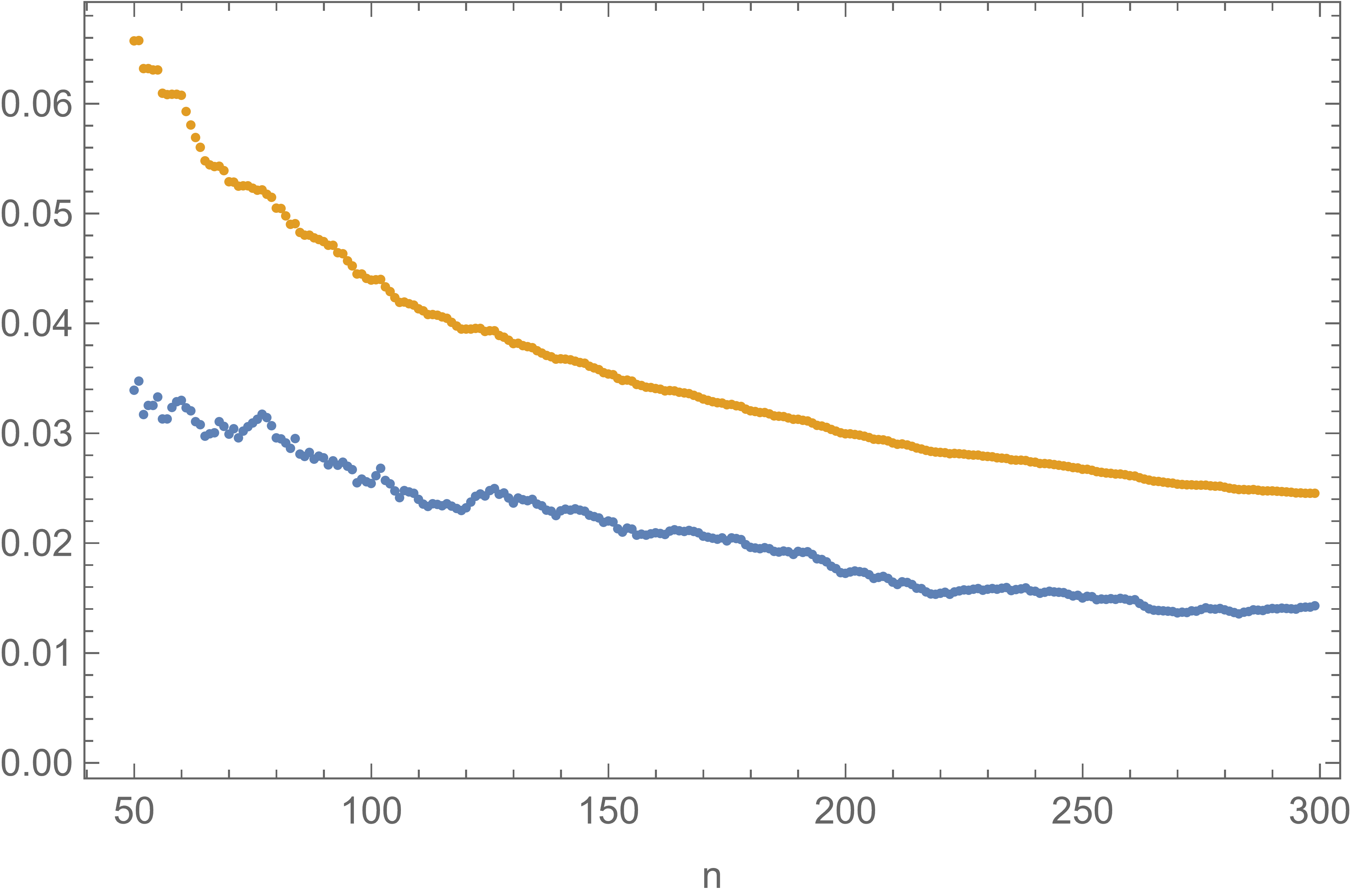
Figure 2: The left resp. right image reports the numerical values of the total variation resp. Wasserstein bound (44) and numerical estimation of the true value of the distance in Example 1 for the posterior mode computed on an average of $5$ Bernoulli samples of sizes $n\in\{50,300\}$, with parameters $p=0.6$, $\tau_{1}=1$ and $\tau_{2}=2$.

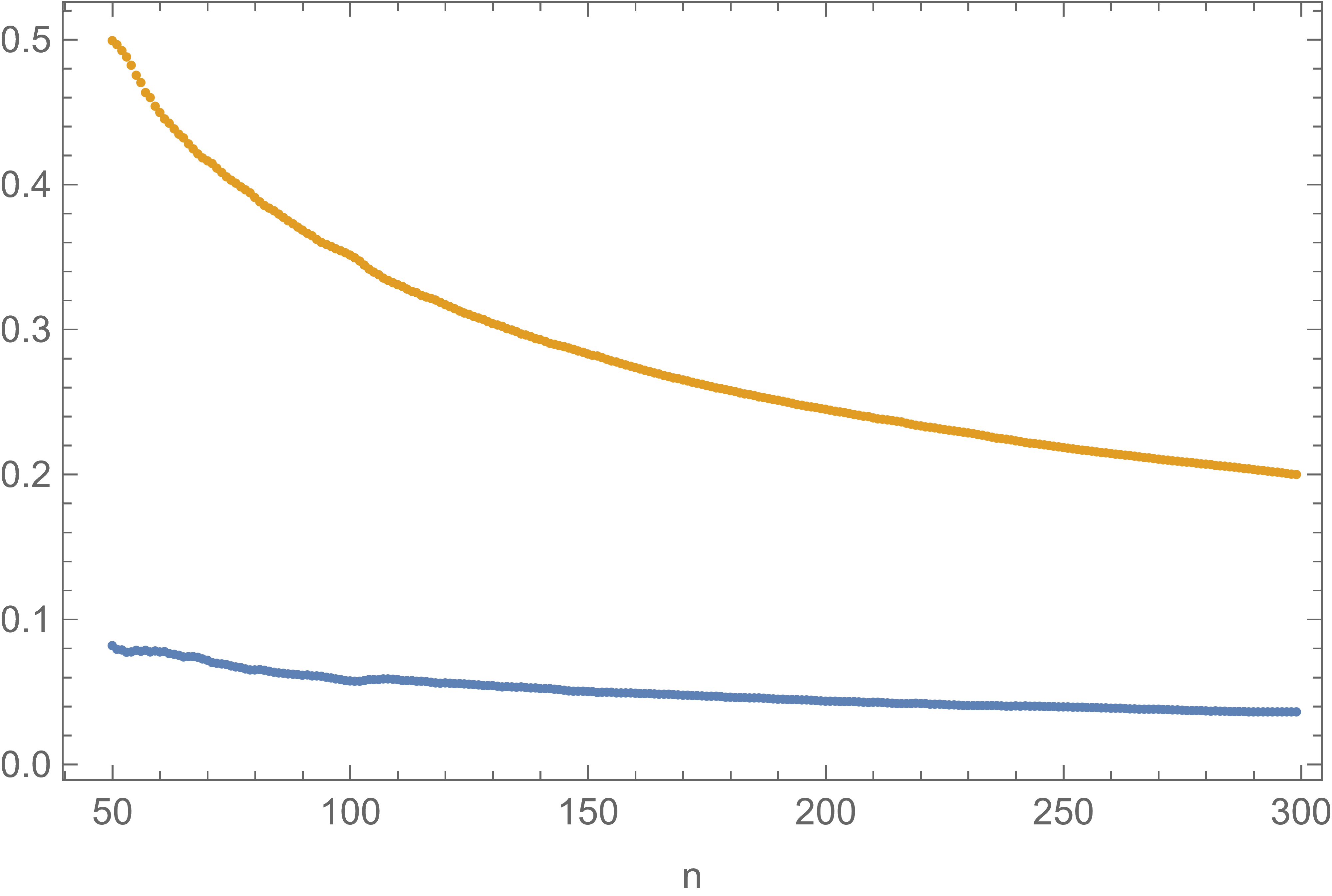
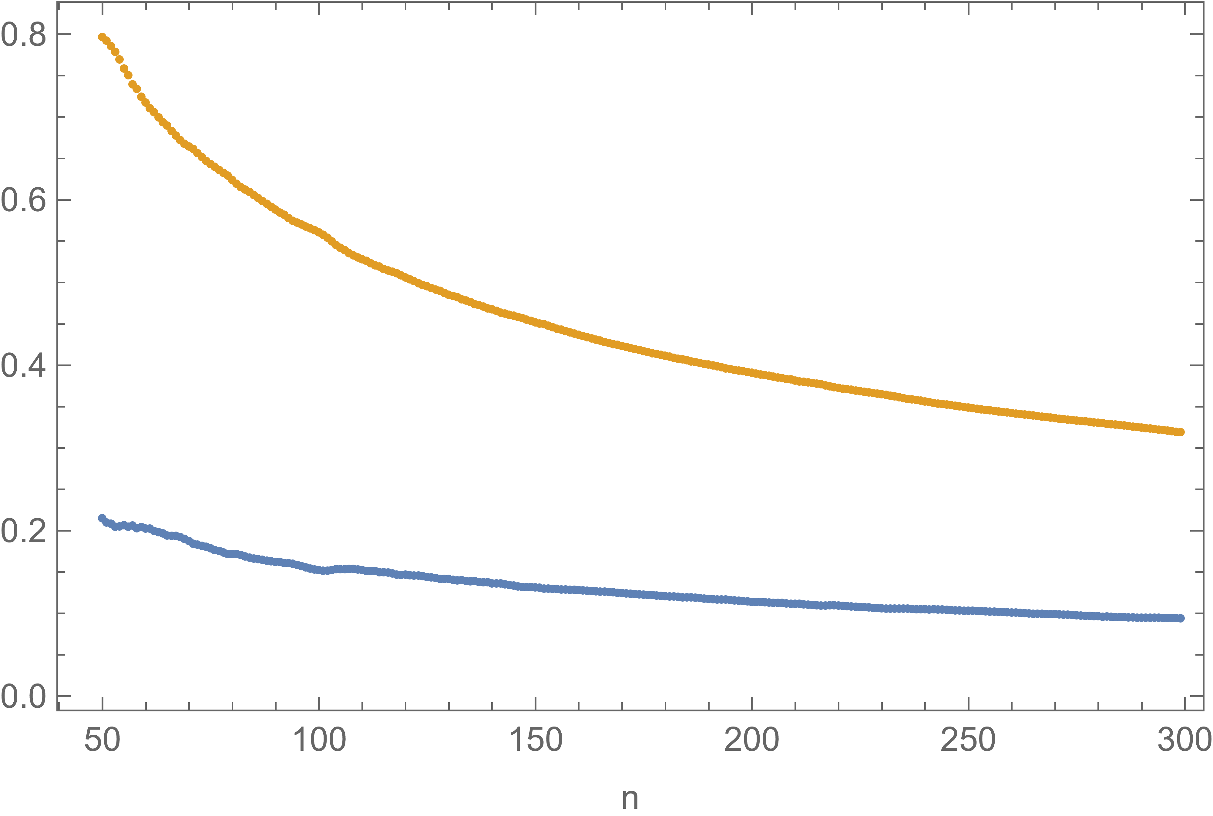
Figure 3: The left resp. right image reports the numerical values of the total variation resp. Wasserstein bound (45) and numerical estimation of the true value of the distance in Example 1 for the MLE (with conjugate prior) computed on an average of $5$ Bernoulli samples of sizes $n\in\{50,300\}$, with parameters $p=0.4$, $\tau_{1}=0.5$ and $\tau_{2}=3$.

Next, we study the normal approximation of the posterior standardized around the MLE. Clearly,

$$\beta^{\prime}(\theta)=\frac{e^{\theta}}{1+e^{\theta}}\mbox{ and }\beta^{\prime\prime}(\theta)=\frac{e^{\theta}}{(1+e^{\theta})^{2}}$$

and, solving $n\beta^{\prime}(\theta)=\sum_{i=1}^{n}x_{i}$, we obtain

$$\hat{\theta}=\log\left(\frac{\bar{x}}{1-\bar{x}}\right),$$

whence

$$\beta^{\prime\prime}(\hat{\theta})=\bar{x}(1-\bar{x}).$$

With $\beta^{\prime\prime\prime}(\theta)=\frac{e^{\theta}(1+e^{\theta})-2e^{2\theta}}{(1+e^{\theta})^{3}}$ we get $|\beta^{\prime\prime\prime}(\theta)|\leq 1/(6\sqrt{3})$. Therefore, $|\hat{\Upsilon}^{\beta}(w)|\leq n/(12\sqrt{3})$ and for any $\eta$ such that Assumptions 0 and $A^{\dagger}$ are satisfied, Theorem 6 gives $d_{\mathrm{Wass}}(\theta^{\dagger},N)\leq\hat{\hat{\Delta}}_{\beta,\eta}(\mathbf{x})$ and $d_{\mathrm{TV}}(\theta^{\dagger},N)\leq\sqrt{\pi/8}\hat{\hat{\Delta}}_{\beta,\eta}(\mathbf{x})$ with

$$\hat{\hat{\Delta}}_{\beta,\eta}(\mathbf{x})\leq\frac{1}{\sqrt{n\bar{x}(1-\bar{x})}}\bigg{(}\frac{1}{12\sqrt{3}}\frac{1}{\bar{x}(1-\bar{x})}\mathbb{E}\left[(\theta^{\dagger})^{2}\right]+\|\eta^{\prime}\|_{\infty}\bigg{)}.$$ (45)

Here we compute

$$\mathbb{E}\left[(\theta^{\dagger})^{2}\right]= n\bar{x}(1-\bar{x})\Bigg{(}\psi^{\prime}(n\bar{x}+\tau_{1})+\psi^{\prime}(n(1-\bar{x})+\tau_{2}-\tau_{1})$$

$$+\Big{(}\psi(n\bar{x}+\tau_{1})-\psi(n(1-\bar{x})+\tau_{2}-\tau_{1})-\log(\bar{x}/(1-\bar{x}))\Big{)}^{2}\Bigg{)}.$$

In the case of the conjugate prior with exponent $\eta(\theta)=-\tau_{1}+\tau_{2}\log(1+e^{\theta})$, the necessary assumptions are satisfied and we have $\eta^{\prime}(\theta)=-\tau_{1}+\tau_{2}e^{\theta}/(1+e^{\theta})$, so that $\|\eta^{\prime}\|_{\infty}\leq\mathrm{max}\{\tau_{1},\tau_{2}-\tau_{1}\}$. For example, with an improper hyperbolic prior $\pi_{0}(\theta)=\cosh(\theta)=\frac{1}{2}(e^{\theta}+e^{-\theta})$ we have $\eta(\theta)=-\log(\cosh(\theta))$ with derivative $\eta^{\prime}(\theta)=-\tanh(\theta)$, which satisfies $\|\eta^{\prime}\|_{\infty}=1$.

We can obtain alternative bounds through Theorem 5, as follows. In the conjugate prior setting described above, Assumptions 0 and $\widehat{\mathrm{A}}$ are satisfied and inequalities (22) and (23) yield

$$d_{\mathrm{TV}}(\theta^{\dagger},N) \leq\frac{\sqrt{\pi}}{\sqrt{8n\bar{x}(1-\bar{x})}}\bigg{(}|\tau_{2}\bar{x}-\tau_{1}|+\frac{|\tau_{2}|\sqrt{\bar{x}(1-\bar{x})}}{\sqrt{n}}\mathbb{E}\big{[}|\theta^{\dagger}|\big{]}+\frac{n+\tau_{2}}{12\sqrt{3}}\frac{1}{n\bar{x}(1-\bar{x})}\mathbb{E}\left[(\theta^{\dagger})^{2}\right]\bigg{)},$$

$$d_{\mathrm{Wass}}(\theta^{\dagger},N) \leq\frac{1}{\sqrt{n\bar{x}(1-\bar{x})}}\bigg{(}|\tau_{2}\bar{x}-\tau_{1}|+\frac{|\tau_{2}|\sqrt{\bar{x}(1-\bar{x})}}{\sqrt{n}}\mathbb{E}\big{[}|\theta^{\dagger}|\big{]}+\frac{n+\tau_{2}}{12\sqrt{3}}\frac{1}{n\bar{x}(1-\bar{x})}\mathbb{E}\left[(\theta^{\dagger})^{2}\right]\bigg{)}.$$

We could also extend these bounds to the general prior case.

B.2 Computations for Example 2

Consider i.i.d. Poisson data with parameter $\mu>0$. We write this distribution as an exponential family with natural parameter $\theta$ by taking

$$\theta=\log\mu,\quad\Theta=(-\infty,\infty),\quad h(x)=x\mbox{ and }\beta(\theta)=e^{\theta}.$$

We consider a conjugate gamma prior on $\mu$ of the form $\pi_{0}(\theta)\propto\exp({-\eta(\theta)})$ with $\eta(\theta)=-\tau_{1}\theta+\tau_{2}e^{\theta}$ for $\tau_{1},\tau_{2}>0$. Then

$$\lambda(\theta)=-\tau_{1}\theta+(n+\tau_{2})e^{\theta},$$

so that

$$\lambda^{\prime}(\theta) =-\tau_{1}+(n+\tau_{2})e^{\theta}\mbox{ and }\lambda^{(k)}(\theta)=(n+\tau_{2})e^{\theta}\mbox{ for all }k\geq 2.$$

Solving $\lambda^{\prime}(w)=\sum_{i=1}^{n}x_{i}$ we obtain

$$\tilde{\theta}=\log\left(\frac{\tau_{1}+n\bar{x}}{n+\tau_{2}}\right)\mbox{ and }\lambda^{(k)}(\tilde{\theta})=\tau_{1}+n\bar{x},\quad k\geq 2.$$

Straightforward integration yields

$$\tilde{\Upsilon}^{\lambda}(w) =(\tau_{1}+n\bar{x})\mathbb{E}\left[Y_{2}\exp\left(\frac{w}{\sqrt{\tau_{1}+n\bar{x}}}Y_{1}Y_{2}\right)\right]$$

$$=\frac{(\tau_{1}+n\bar{x})^{3/2}}{w^{2}}\left(\sqrt{\tau_{1}+n\bar{x}}\left(\exp\left(\frac{w}{\sqrt{\tau_{1}+n\bar{x}}}\right)-1\right)-w\right).$$

Since $|a(\exp(w/a)-1)-w|\leq w^{2}/(2a)\exp(w/a)$ for all $a\geq 0$ and all $w\in\mathbb{R}$, we conclude that

$$|\tilde{\Upsilon}^{\lambda}(w)|\leq\frac{(\tau_{1}+n\bar{x})}{2}\exp\left(\frac{|w|}{\sqrt{\tau_{1}+n\bar{x}}}\right).$$

Since $\lambda^{\prime\prime\prime}(\theta)$ is always positive, Proposition 2 applies and we immediately obtain

$$d_{\mathrm{Wass}}(\theta^{\star},N)=\sqrt{n\bar{x}+\tau_{1}}\left(\log(n+\bar{x}+\tau_{1})-\psi(n+\bar{x}+\tau_{1})\right)\approx\frac{1}{\sqrt{4n\bar{x}+\tau_{1}}},$$

where by $\approx$ we mean that $\lim_{n\to\infty}\sqrt{n}d_{\mathrm{Wass}}(\theta^{\star},N)=1/(2\sqrt{\bar{x}})$ for all admissible values $\tau_{1},\tau_{2}$. For the sake of illustration we compute our Wasserstein distance bound which is obtained simply by incorporating the above result into inequality (14), which gives

$$d_{\mathrm{Wass}}(\theta^{\star},N) \leq\frac{1}{2\sqrt{\tau_{1}+n\bar{x}}}\mathbb{E}\left[(\theta^{\star})^{2}\exp\left(\frac{|\theta^{\star}|}{\sqrt{\tau_{1}+n\bar{x}}}\right)\right].$$

For a total variation distance bound we can either work as above through inequality (15) to get

$$d_{\mathrm{TV}}(\theta^{\star},N) \leq\frac{1}{2\sqrt{\tau_{1}+n\bar{x}}}\mathbb{E}\left[\min\left(\sqrt{\frac{\pi}{8}}(\theta^{\star})^{2},|\theta^{\star}|\right)\exp\left(\frac{|\theta^{\star}|}{\sqrt{\tau_{1}+n\bar{x}}}\right)\right],$$

or work with inequality (16) together with Markov’s inequality. The latter approach yields

$$d_{\mathrm{TV}}(\theta^{\star},N) \leq\frac{1}{2\sqrt{\tau_{1}+n\bar{x}}}\mathbb{E}\left[|\theta^{\star}|\exp\left(\frac{|\theta^{\star}|}{\sqrt{\tau_{1}+n\bar{x}}}\right)\,\Big{|}\,|\theta^{\star}|\leq\epsilon\right]+\frac{3+\sqrt{5}}{2}\frac{\mathbb{E}[|\theta^{\star}|]}{\epsilon}$$

and thus, taking $\epsilon=\sqrt{\tau_{1}+n\bar{x}}$,

$$d_{\mathrm{TV}}(\theta^{\star},N) \leq\frac{1}{2}\bigg{(}\frac{3+\sqrt{5}}{2}+e\bigg{)}\frac{\mathbb{E}[|\theta^{\star}|]}{\sqrt{\tau_{1}+n\bar{x}}}\leq\frac{1}{2}\bigg{(}\frac{3+\sqrt{5}}{2}+e\bigg{)}\frac{\sqrt{\mathbb{E}[(\theta^{\star})^{2}]}}{\sqrt{\tau_{1}+n\bar{x}}}.$$ (46)

We compute as in Example 1

$$A(t)=\log\Gamma(t+\tau_{1})-(t+\tau_{1})\log(n+\tau_{2})$$

and obtain

$$\mathbb{E}[(\theta^{\star})^{2}] =(n\bar{x}+\tau_{1})\left(\psi^{\prime}(n\bar{x}+\tau_{1})+(\psi(n\bar{x}+\tau_{1})-\log(n\bar{x}+\tau_{1}))^{2}\right)$$

$$\leq(n\bar{x}+\tau_{1})\bigg{(}\frac{1}{n\bar{x}+\tau_{1}+1/2}+\frac{1}{(n\bar{x}+\tau_{1})^{2}}-\frac{1}{2(n\bar{x}+\tau_{1})}\bigg{)}$$

$$\leq 1+\frac{1}{n\bar{x}+\tau_{1}}.$$

A numerical illustration of the bounds (46) is provided in Figure 5.

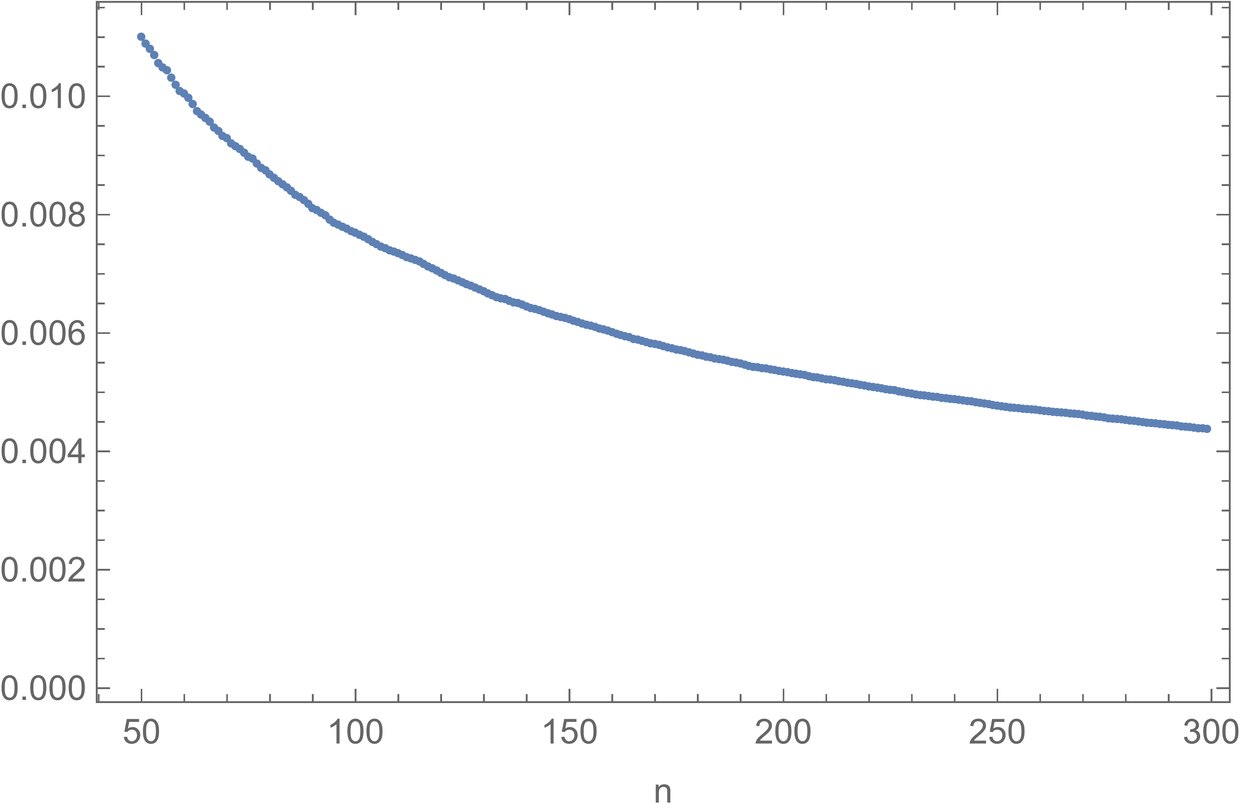
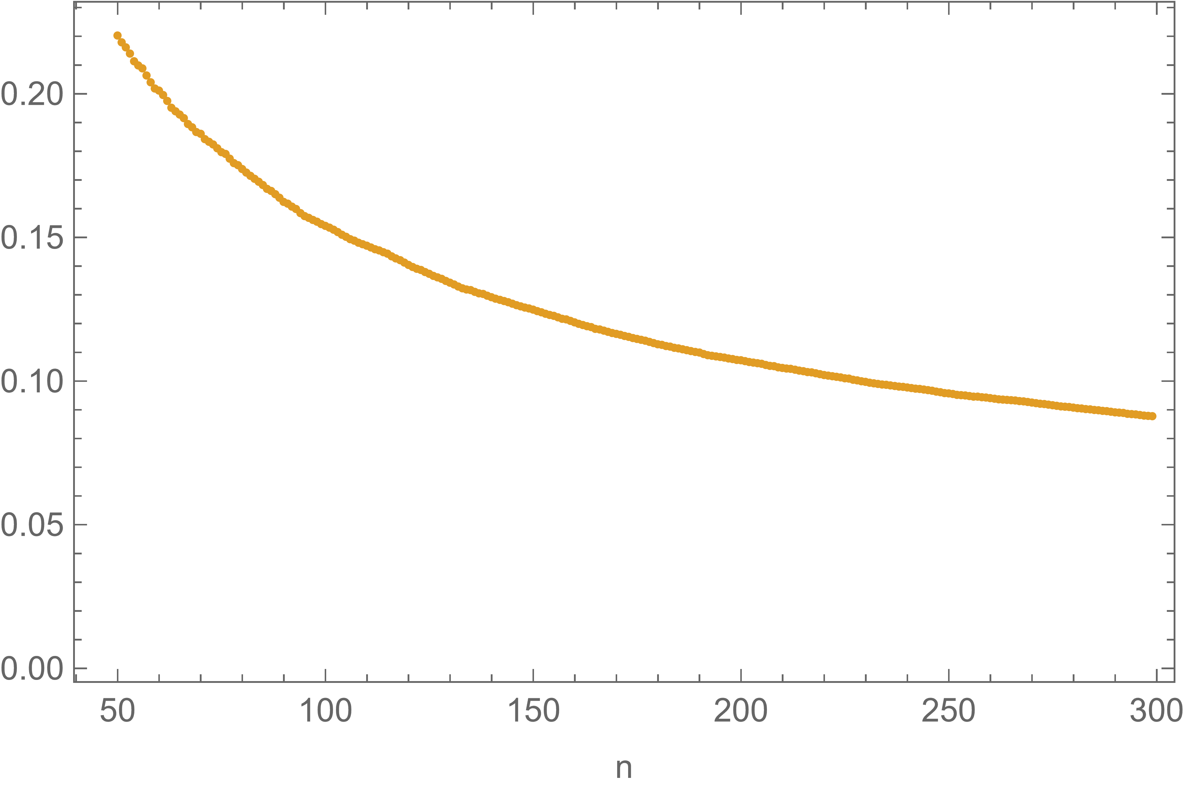
Figure 4: The left image reports the numerical estimation of the true value of the total variation distance and the right image the numerical values of the respective bound (46) in Example 2 computed on an average of $5$ Poisson samples of sizes $n\in\{50,300\}$, with parameters $\mu=3$, $\tau_{1}=8$ and $\tau_{2}=3$.

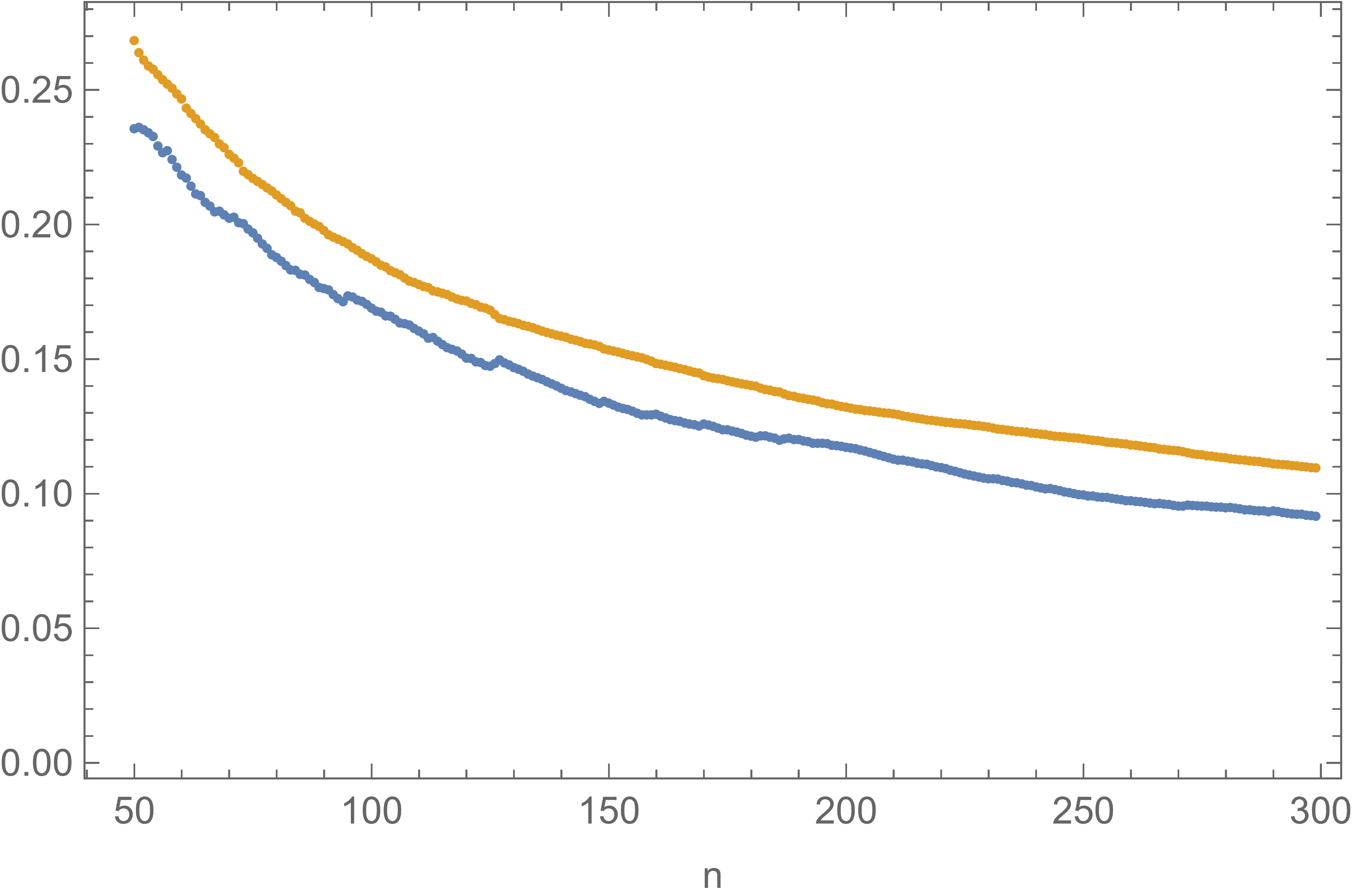
Figure 5: Here we report the numerical estimation of the true value of the total variation distance and the numerical values of the respective bound in Example 3. On the left with respect to the posterior mode and bound (48) and on the right with respect to the MLE and bound (B.3). The estimates are computed on an average of $5$ Gaussian samples of sizes $n\in\{50,300\}$, with parameters $m=1$, $\sigma^{2}=3$, $\tau_{1}=2$ and $\tau_{2}=0.5$.

B.3 Computations for Example 3

Consider i.i.d. normal data with known mean $m$ and unknown variance $\sigma^{2}$. This distribution is written as an exponential family with natural parameter $\theta$ by taking

$$\theta=\sigma^{-2},\quad\Theta=(0,\infty),\quad h(x)=-(x-m)^{2}/2\mbox{ and }\beta(\theta)=-(1/2)\log\theta.$$

We consider a conjugate gamma prior on $\theta$ of the form $\pi_{0}(\theta)\propto\exp({-\eta(\theta)})$, where $\eta(\theta)=\tau_{1}\theta-\tau_{2}\log\theta$ for $\tau_{1}>0$ and $\tau_{2}>-1$. The posterior distribution $\theta$ has a gamma distribution with shape parameter $n/2+\tau_{2}+1$, and so Assumption 0 is satisfied if $n+2\tau_{2}>0$. Then

$$\lambda(\theta)=\tau_{1}\theta-(\tau_{2}+n/2)\log\theta,$$

so that, for $n\geq 2$,

$$\lambda^{\prime}(\theta)=\tau_{1}-\frac{n/2+\tau_{2}}{\theta},\quad\lambda^{\prime\prime}(\theta)=\frac{n/2+\tau_{2}}{\theta^{2}}\mbox{ and }\lambda^{\prime\prime\prime}(\theta)=-\frac{n+2\tau_{2}}{\theta^{3}}.$$

Solving $\lambda^{\prime}(w)=\sum_{i=1}^{n}x_{i}$ we obtain

$$\tilde{\theta}=\frac{n+2\tau_{2}}{n\tilde{s}^{2}+2\tau_{1}}\mbox{ so that }\lambda^{\prime\prime}(\tilde{\theta})=\frac{(n\tilde{s}^{2}+2\tau_{1})^{2}}{2(n+2\tau_{2})},$$

where we let $n\tilde{s}^{2}=\sum_{i=1}^{n}(x_{i}-m)^{2}$. Straightforward integration yields

$$\tilde{\Upsilon}^{\lambda}(w)=-\frac{(n\tilde{s}^{2}+2\tau_{1})^{3}}{2(n+2\tau_{2})^{2}\left(1+\sqrt{2}w\sqrt{\frac{1}{n+2\tau_{2}}}\right)}.$$

Applying inequality (15) gives, after some straightforward simplifications

$$d_{\mathrm{TV}}(\theta^{\star},N) \leq\mathbb{E}\left[\min\left(\sqrt{\frac{\pi}{8}}(\theta^{\star})^{2},|\theta^{\star}|\right)\left|\frac{1}{\sqrt{n/2+\tau_{2}}+\theta^{\star}}\right|\right]\leq\sqrt{\frac{\pi}{8}}\frac{n\tilde{s}^{2}+2\tau_{1}}{\sqrt{2(n+2\tau_{2})}}\mathbb{E}\left[\frac{(\theta-\tilde{\theta})^{2}}{\theta}\right].$$

As $\theta$ follows a gamma distribution, we have the simple formulas

$$\mathbb{E}[\theta]=\frac{n+2\tau_{2}+2}{n\tilde{s}^{2}+2\tau_{1}},\quad\mathbb{E}[\theta^{-1}]=\frac{n\tilde{s}^{2}+2\tau_{1}}{n+2\tau_{2}}.$$ (47)

It follows that $\mathbb{E}[{(\theta-\tilde{\theta})^{2}}/{\theta}]={2}/{(n\tilde{s}^{2}+2\tau_{1})}.$ Substituting this in the last inequality, yields

$$d_{\mathrm{TV}}(\theta^{\star},N) \leq\frac{\sqrt{\pi}}{2}\frac{1}{\sqrt{n+2\tau_{2}}}.$$ (48)

Similarly, inequality (14) yields the bound $d_{\mathrm{Wass}}(\theta^{\star},N)\leq\sqrt{2}/\sqrt{n+2\tau_{2}}$. Also, we can use inequality (17) to obtain a lower bound for the Wasserstein distance:

$$d_{\mathrm{Wass}}(\theta^{\star},N)\geq\frac{\phi}{\sqrt{2(n+2\tau_{2})}}\bigg{(}\frac{n+2\tau_{2}+2}{\phi}-\frac{n+2\tau_{2}}{\phi}\bigg{)}=\frac{\sqrt{2}}{\sqrt{n+2\tau_{2}}},$$

where we let $\phi=n\tilde{s}^{2}+2\tau_{1}$. From the upper and lower bounds, we thus deduce the equality

$$d_{\mathrm{Wass}}(\theta^{\star},N)=\frac{\sqrt{2}}{\sqrt{n+2\tau_{2}}}.$$

We now obtain bounds for the standardised posterior $\theta^{\dagger}$. Some of the quantities required to apply inequalities (22) and (23) have already been calculated. We note that also $\hat{\theta}=1/\tilde{s}^{2}$, $\eta^{\prime}(\hat{\theta})=\tau_{1}-\tau_{2}\tilde{s}^{2}$, $\eta^{\prime\prime}(\hat{\theta})=\tau_{2}\tilde{s}^{4}$ and $\beta^{\prime\prime}(\hat{\theta})=\tilde{s}^{4}/(2n^{2})$. With a similar calculation to the one we used for the standardised posterior $\theta^{\star}$, and making use of the expectations in (47), we obtain the bound

$$d_{\mathrm{TV}}(\theta^{\dagger},N) \leq\sqrt{\frac{\pi}{8n\beta^{\prime\prime}(\hat{\theta})}}\bigg{\{}|\eta^{\prime}(\hat{\theta})|+\eta^{\prime\prime}(\hat{\theta})(\mathbb{E}[\theta]+\hat{\theta})+\frac{n+2\tau_{2}}{2\hat{\theta}^{2}}\mathbb{E}\bigg{[}\frac{(\theta-\hat{\theta})^{2}}{\theta}\bigg{]}\bigg{\}}$$

$$=\frac{\sqrt{\pi}}{2\tilde{s}^{2}\sqrt{n}}\bigg{\{}\big{|}\tau_{2}\tilde{s}^{2}-\tau_{1}\big{|}+|\tau_{2}|\tilde{s}^{2}\bigg{(}\frac{n+2\tau_{2}+2}{n\tilde{s}^{2}+2\tau_{1}}+\frac{1}{\tilde{s}^{2}}\bigg{)}$$

$$\quad+\frac{2(\tau_{2}n\tilde{s}^{2}-n\tau_{1})^{2}+(n+2\tau_{2})(n\tilde{s}^{2})^{2}}{n^{2}(n\tilde{s}^{2}+2\tau_{1})}\bigg{\}},$$ (49)

where in the first step we used that $\mathbb{E}[|\theta^{\dagger}|]\leq(n\beta^{\prime\prime}(\hat{\theta}))^{1/2}(\mathbb{E}[\theta]+\hat{\theta})$. We can also use Theorem 6, together with similar calculations to the ones above, to get

$$d_{\mathrm{TV}}(\theta^{\dagger},N) \leq\sqrt{\frac{\pi}{8n\beta^{\prime\prime}(\hat{\theta})}}\bigg{\{}\frac{n}{2\hat{\theta}^{2}}\mathbb{E}\bigg{[}\frac{(\theta-\hat{\theta})^{2}}{\theta}\bigg{]}+|\mathbb{E}[\eta^{\prime}(\hat{\theta})]|\bigg{\}}$$

$$=\frac{\sqrt{\pi}}{2\tilde{s}^{2}\sqrt{n}}\bigg{\{}\frac{2(\tau_{2}n\tilde{s}^{2}-n\tau_{1})^{2}+(n+2\tau_{2})(n\tilde{s}^{2})^{2}}{n(n+2\tau_{2})(n\tilde{s}^{2}+2\tau_{1})}+\frac{\sqrt{2n}|\tau_{2}|(n\tilde{s}^{2}+2\tau_{1})}{(n+2\tau_{2})n\tilde{s}^{2}}\bigg{\}}=:B_{n},$$

where we used that $\eta^{\prime}(\theta)=-\tau_{2}/\theta$ and then calculated $\mathbb{E}[\theta^{-1}]$ using (47). Similarly, we can obtain an upper bound on the Wasserstein distance, whilst a lower bound can be calculated using the inequality $d_{\mathrm{Wass}}(\theta^{\dagger},N)\geq(n\beta^{\prime\prime}(\hat{\theta}))^{1/2}|\mathbb{E}[\theta]-\hat{\theta}|$ together with the formula for $\mathbb{E}[\theta]$ from (47). This gives the two-sided inequality

$$\sqrt{n}\frac{\sqrt{2}|(\tau_{2}+1)\tilde{s}^{2}-\tau_{1}|}{(n\tilde{s}^{2}+2\tau_{1})}\leq d_{\mathrm{Wass}}(\theta^{\dagger},N)\leq\sqrt{\frac{8}{\pi}}B_{n}.$$

As in the previous examples, the quality of the bounds is illustrated over an average of 5 sample; see Figure 5. We observe the expected behavior.

B.4 Computations for Example 5

Consider i.i.d.  negative binomial data with density

$$p_{1}(x|r,p) =\binom{x+r-1}{x}(1-p)^{r}p^{x}=\mathrm{exp}\left\{x\log p+\log\binom{x+r-1}{x}+r\log(1-p)\right\}.$$

We suppose $r$ is known, and $p$ is the parameter of interest. Then $h(x)=x$, $g(x)=\log\binom{x+r-1}{x}$ and the natural parameter is $\theta=\log p$; we take $\Theta=(-\infty,0)$. Fix, for $\tau_{1}>0$ and $\tau_{2}>-1$, a (conjugate) prior on $\theta$ of the form $\pi_{0}(\theta)\propto\exp(-\eta(\theta))$, where $\eta(\theta)=-{\theta\tau_{1}}-\tau_{2}\log(1-e^{\theta})$. Therefore $\lambda(\theta)=-{\theta\tau_{1}}-(nr+\tau_{2})\log(1-e^{\theta})$. It then holds that

$$\lambda^{\prime}(\theta) =-\tau_{1}+(nr+\tau_{2})\frac{e^{\theta}}{1-e^{\theta}}\mbox{ and }\tilde{\theta}=\log\left(\frac{n\bar{x}+\tau_{1}}{n\bar{x}+\tau_{1}+\tau_{2}+nr}\right),$$

$$\lambda^{\prime\prime}(\theta) =(nr+\tau_{2})\frac{e^{\theta}}{(1-e^{\theta})^{2}}\mbox{ and }\lambda^{\prime\prime}(\tilde{\theta})=\frac{(n\bar{x}+\tau_{1})(n\bar{x}+\tau_{1}+\tau_{2}+nr)}{(nr+\tau_{2})},$$

$$\lambda^{\prime\prime\prime}(\theta) =-\frac{1}{8}(nr+\tau_{2})\mathrm{csch}^{4}(\theta/2)\sinh(\theta).$$

Then (16) together with Markov’s inequality gives

$$d_{\mathrm{TV}}(\theta^{\star},N) \leq\frac{1}{(\lambda^{\prime\prime}(\tilde{\theta}))^{3/2}}\mathbb{E}\left[\left|\theta^{\star}\tilde{\Upsilon}^{\lambda}(w)\right|\,\Big{|}\,|\theta^{\star}|\leq\epsilon\right]+\frac{3+\sqrt{5}}{2}\frac{\mathbb{E}[|\theta^{\star}|]}{\epsilon},$$ (50)

where $\tilde{\Upsilon}^{\lambda}(w)=\mathbb{E}[Y_{2}\lambda^{\prime\prime\prime}(Y_{1}Y_{2}{w}/(\lambda^{\prime\prime}(\tilde{\theta}))^{1/2}+\tilde{\theta})]$. We shall take $\epsilon=-\tilde{\theta}(\lambda^{\prime\prime}(\tilde{\theta}))^{1/2}/2>0$. The second term is easily bounded, so we deal with it first:

$$\frac{\mathbb{E}[|\theta^{\star}|]}{\epsilon}=-\frac{2\mathbb{E}[|\theta^{\star}|]}{\tilde{\theta}\sqrt{\lambda^{\prime\prime}(\tilde{\theta})}}=\frac{2}{\sqrt{\lambda^{\prime\prime}(\tilde{\theta})}}\bigg{(}\log\bigg{(}\frac{n\bar{x}+\tau_{1}+\tau_{2}+nr}{n\bar{x}+\tau_{1}}\bigg{)}\bigg{)}^{-1}\mathbb{E}[|\theta^{\star}|].$$ (51)

We now bound the expectation in the first term, which we denote by $A$:

$$A =\frac{nr+\tau_{2}}{8}\mathbb{E}\left[\left|\theta^{\star}\ \mathbb{E}\left[Y_{2}\operatorname{csch}^{4}\left(\frac{\tilde{\theta}}{2}+\frac{\theta^{\star}Y_{1}Y_{2}}{2\sqrt{\lambda^{\prime\prime}(\tilde{\theta})}}\right)\sinh\left(\frac{\tilde{\theta}}{2}+\frac{\theta^{\star}Y_{1}Y_{2}}{2\sqrt{\lambda^{\prime\prime}(\tilde{\theta})}}\right)\,\Big{|}\,\theta^{\star}\right]\right|\,\Big{|}\,|\theta^{\star}|\leq-\frac{\tilde{\theta}\sqrt{\lambda^{\prime\prime}(\tilde{\theta})}}{2}\right]$$

$$\leq\frac{nr+\tau_{2}}{8}\mathbb{E}\left[\left|\theta^{\star}\mathbb{E}\left[\left|Y_{2}\operatorname{csch}^{4}\big{(}\tilde{\theta}/4\big{)}\sinh\big{(}3\tilde{\theta}/2\big{)}\right|\right]\right|\right]=\frac{nr+\tau_{2}}{16}\operatorname{csch}^{4}\big{(}\tilde{\theta}/4\big{)}\sinh\big{(}-3\tilde{\theta}/2\big{)}\mathbb{E}[|\theta^{\star}|].$$ (52)

We note the simple formula

$$\operatorname{csch}^{4}\bigg{(}\frac{\log(x)}{4}\bigg{)}\sinh\bigg{(}-\frac{3\log(x)}{2}\bigg{)}=\frac{8(1-x^{3})}{\sqrt{x}(1-\sqrt{x})^{4}},\quad 0<x<1.$$

Making use of this formula and substituting the formula for the posterior mode $\tilde{\theta}$ into inequality (52) yields the bound

$$A\leq\frac{(nr+\tau_{2})((n\bar{x}+\tau_{1}+\tau_{2}+nr)^{3}-(n\bar{x}+\tau_{1})^{3})}{2\sqrt{(\sum_{i}x_{i}+\tau_{1})(n\bar{x}+\tau_{1}+\tau_{2}+nr)}(\sqrt{n\bar{x}+\tau_{1}+\tau_{2}+nr}-\sqrt{n\bar{x}+\tau_{1}})^{4}}\mathbb{E}[|\theta^{\star}|].$$ (53)

Applying inequalities (51) and (53) into (50), together with the formula for $\lambda^{\prime\prime}(\tilde{\theta})$, now yields

$$d_{\mathrm{TV}}(\theta^{\star},N) \leq\frac{\sqrt{nr+\tau_{2}}\mathbb{E}[|\theta^{\star}|]}{2\sqrt{(n\bar{x}+\tau_{1})(nr+n\bar{x}+\tau_{1}+\tau_{2})}}\bigg{\{}2(3+\sqrt{5})\bigg{(}\log\bigg{(}\frac{n\bar{x}+\tau_{1}+\tau_{2}+nr}{n\bar{x}+\tau_{1}}\bigg{)}\bigg{)}^{-1}$$

$$\quad+\frac{(nr+\tau_{2})^{2}((n\bar{x}+\tau_{1}+\tau_{2}+nr)^{3}-(n\bar{x}+\tau_{1})^{3})}{(n\bar{x}+\tau_{1})^{3/2}(n\bar{x}+\tau_{1}+\tau_{2}+nr)^{3/2}(\sqrt{n\bar{x}+\tau_{1}+\tau_{2}+nr}-\sqrt{n\bar{x}+\tau_{1}})^{4}}\bigg{\}}.$$

We bound $\mathbb{E}[|\theta^{\star}|]$ by $\sqrt{\mathbb{E}[(\theta^{\star})^{2}]}$. Proceeding the same way as in Examples 1 and 2, we obtain

$$\mathbb{E}[\theta] =\psi(n\bar{x}+\tau_{1})-\psi(nr+n\bar{x}+\tau_{1}+\tau_{2}+1)\approx\log\left(\frac{n\bar{x}+\tau_{1}}{nr+n\bar{x}+\tau_{1}+\tau_{2}}\right)=\tilde{\theta},$$

$$\mathbb{E}[\theta^{2}] =\psi^{\prime}(n\bar{x}+\tau_{1})-\psi^{\prime}(nr+n\bar{x}+\tau_{1}+\tau_{2}+1)+\Big{(}\psi(n\bar{x}+\tau_{1})-\psi(nr+n\bar{x}+\tau_{1}+\tau_{2}+1)\Big{)}^{2}$$

$$\approx\frac{1}{n\bar{x}+\tau_{1}}+\tilde{\theta}^{2},$$

and therefore

$$\mathbb{E}[(\theta^{\star})^{2}]=\lambda^{\prime\prime}(\tilde{\theta})\Big{(}\mathbb{E}[\theta^{2}]-2\tilde{\theta}\mathbb{E}[\theta]+\tilde{\theta}^{2}\Big{)}\approx\frac{n\bar{x}+\tau_{1}+\tau_{2}+nr}{nr+\tau_{2}}.$$

B.5 Computations for Example 6

Consider i.i.d. multinomial data with parameters $(p_{1},\ldots,p_{k})^{\intercal}$ and individual likelihood

$$p_{1}(x|p)=\prod_{j=1}^{k}p_{j}^{x_{j}}=\mathrm{exp}\Bigg{\{}\sum_{j=1}^{k}x_{j}\log(p_{j})\Bigg{\}},$$ (54)

where $0<p_{1},\ldots,p_{k}<1$ with $\sum_{j=1}^{k}p_{j}=1$, and $x_{1},\ldots,x_{k}\in\{0,1\}$ with $\sum_{j=1}^{k}x_{j}=1$. We express the likelihood (54) as an exponential family by writing

$$p_{1}(x|p) =\mathrm{exp}\Bigg{\{}\sum_{j=1}^{k-1}x_{j}\log(p_{j})+\Bigg{(}1-\sum_{j=1}^{k-1}x_{j}\Bigg{)}\log(p_{k})\Bigg{\}}=\mathrm{exp}\Bigg{\{}\sum_{j=1}^{k-1}x_{j}\log\left(\frac{p_{j}}{p_{k}}\right)+\log(p_{k})\Bigg{\}},$$

so $h_{j}(x_{j})=x_{j}$, $g(x)=0$ and the natural parameter is $\theta=(\theta_{1},\ldots,\theta_{k-1})^{\intercal}$, where $\theta_{j}=\log(p_{j}/p_{k})$, $j=1,\ldots,k-1$, and $\Theta=\mathbb{R}^{k-1}$. Expressing the density in terms of $\theta$, we get $p_{j}(\theta)=p_{k}e^{\theta_{j}}$. Also, since $\sum_{j=1}^{k}p_{j}=1$, we obtain that $p_{k}+p_{k}\sum_{j=1}^{k-1}e^{\theta_{j}}=1$, so that $p_{k}=(1+\sum_{j=1}^{k-1}e^{\theta_{j}})^{-1}$. Thus, $\beta(\theta)=-\log(p_{k}(\theta))=\log(1+\sum_{j=1}^{k-1}e^{\theta_{j}}).$ Fix a (conjugate) Dirichlet prior on $p=(p_{1},\ldots,p_{k-1})^{\intercal}$ of the form $\pi_{0}(p)\propto p_{k}^{\tau_{k}-\sum_{j=1}^{k-1}\tau_{j}}\prod_{j=1}^{k-1}p_{j}^{\tau_{j}}$ for $\tau_{1},\ldots,\tau_{k-1}>-1$ and $\tau_{k}>\sum_{j=1}^{k-1}\tau_{j}-1$, so that $\pi_{0}(\theta)\propto e^{-\eta(\theta)}$, where $\eta(\theta)=-\sum_{j=1}^{k-1}\tau_{j}\theta_{j}+\tau_{k}\log(1+\sum_{j=1}^{k-1}e^{\theta_{j}}).$ Therefore $\lambda(\theta)=-\sum_{j=1}^{k-1}\tau_{j}\theta_{j}+(n+\tau_{k})\log(1+\sum_{j=1}^{k-1}e^{\theta_{j}}).$ It holds that

$$\partial_{\theta_{u}}\lambda(\theta)=-\tau_{u}+(n+\tau_{k})\frac{e^{\theta_{u}}}{1+\sum_{j=1}^{k-1}e^{\theta_{j}}}.$$

From Fact 1a, it follows that the posterior mode $\tilde{\theta}$ solves the system of equations $\partial_{\theta_{j}}\lambda(\theta)-\sum_{i=1}^{n}h_{j}(x_{i})=0$, for $j=1,\ldots,k-1$. Solving this yields that $\tilde{\theta}=(\tilde{\theta}_{1},\ldots,\tilde{\theta}_{k-1})^{\intercal}$, where

$$\tilde{\theta}_{u}=\log\bigg{(}\frac{\tau_{u}+\sum_{i=1}^{n}x_{i,u}}{n+\tau_{k}-\sum_{j=1}^{k-1}\tau_{j}-\sum_{i=1}^{n}\sum_{j=1}^{k-1}x_{i,j}}\bigg{)},\quad u=1,\ldots,k-1.$$

Also, the second-order partial derivatives are given by

$$\partial_{\theta_{u},\theta_{u}}\lambda(\theta)=(n+\tau_{k})\frac{e^{\theta_{u}}(1+\sum_{j=1}^{k-1}e^{\theta_{j}}-e^{\theta_{u}})}{(1+\sum_{j=1}^{k-1}e^{\theta_{j}})^{2}},\quad\partial_{\theta_{u},\theta_{v}}\lambda(\theta)=-(n+\tau_{k})\frac{e^{\theta_{u}+\theta_{v}}}{(1+\sum_{j=1}^{k-1}e^{\theta_{j}})^{2}},\quad u\not=v,$$

and

$$\partial_{\theta_{u},\theta_{u}}\lambda(\tilde{\theta}) =\frac{(\tau_{u}+\sum_{i}x_{i,u})(n+\tau_{k}-\tau_{u}-\sum_{i}x_{i,u})}{n+\tau_{k}},$$ (55)

$$\partial_{\theta_{u},\theta_{v}}\lambda(\tilde{\theta}) =-\frac{(\tau_{u}+\sum_{i}x_{i,u})(\tau_{v}+\sum_{i}x_{i,v})}{n+\tau_{k}},\quad u\not=v.$$ (56)

The entries in (55) and (56) correspond to the elements in the $(k-1)\times(k-1)$ Hessian matrix $\mathbf{H}_{\lambda}(\tilde{\theta})$. For general $k\geq 2$, it is not possible to give simple closed-form formulas for the elements of $(\mathbf{H}_{\lambda}(\tilde{\theta}))^{-1/2}$. Therefore to provide a bound with an explicit $O(n^{-1/2})$ dependence, we define a $(k-1)\times(k-1)$ matrix $B_{k}$ by $(B_{k})_{u,v}=b_{u,v}$, where

$$b_{u,u}=\frac{(\tau_{u}+\sum_{i}x_{i,u})(n+\tau_{k}-\tau_{u}-\sum_{i}x_{i,u})}{(n+\tau_{k})n},\quad b_{u,v}=-\frac{(\tau_{u}+\sum_{i}x_{i,u})(\tau_{v}+\sum_{i}x_{i,v})}{(n+\tau_{k})n},\quad u\not=v.$$

The entries of $B_{k}$ are of order $O(1)$ with respect to $n$, and we have that $\mathbf{H}_{\lambda}(\tilde{\theta})=nB_{k}$. Now, we define $C_{k}=B_{k}^{-1/2}$, with elements $c_{i,j}=n^{1/2}a_{i,j}=O(1)$, where $a_{i,j}=((\mathbf{H}_{\lambda}(\tilde{\theta}))^{-1/2})_{i,j}$ for $1\leq i,j\leq k-1$. We also let $\|C_{k}\|_{\infty}=\mathrm{max}_{1\leq i\leq k-1}\sum_{j=1}^{k-1}|c_{i,j}|$, the absolute row sum norm of $C$. Note that $\|C_{k}\|_{\infty}=O(1)$, and we have that $R_{u}^{\lambda}\leq\tilde{R}_{u}^{\lambda}\leq\|C_{k}\|_{\infty}/\sqrt{n}$, for $u=1,\ldots,k-1$.

Moving onto the third-order partial derivatives, we have

$$\partial_{\theta_{u},\theta_{u},\theta_{u}}\lambda(\theta) =(n+\tau_{k})\frac{e^{\theta_{u}}(1+\sum_{j=1}^{k-1}e^{\theta_{j}}-e^{\theta_{u}})(1+\sum_{j=1}^{k-1}e^{\theta_{j}}-2e^{\theta_{u}})}{(1+\sum_{j=1}^{k-1}e^{\theta_{j}})^{3}},$$

$$\partial_{\theta_{u},\theta_{u},\theta_{v}}\lambda(\theta) =-(n+\tau_{k})\frac{e^{\theta_{u}+\theta_{v}}(1+\sum_{j=1}^{k-1}e^{\theta_{j}}-2e^{\theta_{u}})}{(1+\sum_{j=1}^{k-1}e^{\theta_{j}})^{3}},\quad u\not=v,$$

$$\partial_{\theta_{u},\theta_{v},\theta_{w}}\lambda(\theta) =(n+\tau_{k})\frac{2e^{\theta_{u}+\theta_{v}+\theta_{w}}}{(1+\sum_{j=1}^{k-1}e^{\theta_{j}})^{3}},\quad u\not=v\not=w.$$

It is straightforward to see that $|\partial_{u,v,w}\lambda(y)|\leq 2(n+\tau_{k})$ for all $1\leq u,v,w\leq k-1$ and all $y\in\mathbb{R}^{k-1}$.

Finally, applying Theorem 1 yields the bounds

$$d_{\mathrm{TV}}(\theta^{\star},N) \leq\frac{2\sqrt{2\pi}}{3}(k-1)\|C_{k}\|_{\infty}^{3}\frac{(n+\tau_{k})}{n^{3/2}}\sum_{u=1}^{k-1}\sum_{v=1}^{k-1}\mathbb{E}[|\theta_{u}^{\star}\theta_{v}^{\star}|]$$

$$\leq\frac{2\sqrt{2\pi}}{3}(k-1)^{2}\|C_{k}\|_{\infty}^{3}\frac{(n+\tau_{k})}{n^{3/2}}\sum_{u=1}^{k-1}\mathbb{E}[(\theta_{u}^{\star})^{2}],$$

$$d_{\mathrm{Wass}}(\theta^{\star},N) \leq(k-1)^{2}\|C_{k}\|_{\infty}^{3}\frac{(n+\tau_{k})}{n^{3/2}}\sum_{u=1}^{k-1}\mathbb{E}[(\theta_{u}^{\star})^{2}],$$

where in obtaining the second inequality we used the basic inequality $ab\leq(a^{2}+b^{2})/2$. In order to calculate the expectations above we need to compute expectations of the posterior distribution which are given in [24, Proposition 2], i.e.

$$\mathbb{E}[\theta_{u}]= \psi(\tau_{u})-\psi\bigg{(}\tau_{k}-\sum_{i=1}^{k-1}\tau_{i}\bigg{)},$$

$$\mathbb{E}[\theta_{u}^{2}]= \psi^{\prime}(\tau_{u})+\psi^{\prime}\bigg{(}\tau_{k}-\sum_{i=1}^{k-1}\tau_{i}\bigg{)}+\Bigg{(}\psi(\tau_{u})-\psi\bigg{(}\tau_{k}-\sum_{i=1}^{k-1}\tau_{i}\bigg{)}\Bigg{)}^{2},$$

$$\mathbb{E}[\theta_{u}\theta_{v}]= \psi^{\prime}\bigg{(}\tau_{k}-\sum_{i=1}^{k-1}\tau_{i}\bigg{)}$$

$$+\Bigg{(}\psi(\tau_{u})-\psi\bigg{(}\tau_{k}-\sum_{i=1}^{k-1}\tau_{i}\bigg{)}\Bigg{)}\Bigg{(}\psi(\tau_{v})-\psi\bigg{(}\tau_{k}-\sum_{i=1}^{k-1}\tau_{i}\bigg{)}\Bigg{)},\qquad v\neq u=1,\ldots,k-1.$$

Hence we have

$$\sum_{i=1}^{k-1}\mathbb{E}\big{[}(\theta^{\star}_{i})^{2}\big{]}=\mathrm{Tr}\big{(}\big{(}\mathbf{H}_{\lambda}(\tilde{\theta})\big{)}^{1/2}\mathbb{E}\big{[}\theta\theta^{\intercal}-2\theta\tilde{\theta}^{\intercal}+\tilde{\theta}\tilde{\theta}^{\intercal}\big{]}\big{(}\mathbf{H}_{\lambda}(\tilde{\theta})\big{)}^{1/2}\big{)}.$$

When $k=3$, we can give an explicit formula for $\|C_{3}\|_{\infty}$. Indeed, by inequality (12), $\|C_{3}\|_{\infty}\leq\sqrt{2/\lambda_{\mathrm{min}}}$, where $\lambda_{\mathrm{min}}>0$ is the smallest eigenvalue of $B_{3}$. The eigenvalues of the $2\times 2$ symmetric matrix $B_{3}$ are solutions to the characteristic equation $0=\mathrm{det}(B_{3}-\lambda I_{2})=\lambda^{2}-(b_{1,1}+b_{2,2})\lambda+b_{1,1}b_{2,2}-b_{1,2}^{2}$. Solving using the quadratic formula and simplifying yields $\lambda=(b_{1,1}+b_{2,2}\pm((b_{1,1}-b_{2,2})^{2}+4b_{1,2}^{2})^{1/2})/2$. Since $B_{3}$ is positive definite (it is equal up to a constant to the positive definite matrix $\mathbf{H}_{\lambda}(\tilde{\theta})$), its eigenvalues are positive real numbers, and as $b_{1,1}>0$ and $b_{2,2}>0$, the smallest eigenvalue is obtained by taking the negative square root:

$$\lambda_{\mathrm{min}} =\frac{1}{2n(n+\tau_{3})}\bigg{(}(\tau_{1}+\sum_{i}x_{i,1})(n+\tau_{3}-\tau_{1}-\sum_{i}x_{i,1})+(\tau_{2}+\sum_{i}x_{i,2})(n+\tau_{3}-\tau_{2}-\sum_{i}x_{i,2})$$

$$\quad-\Big{(}\Big{(}((\tau_{1}+\sum_{i}x_{i,1})(n+\tau_{3}-\tau_{1}-\sum_{i}x_{i,1})-(\tau_{2}+\sum_{i}x_{i,2})(n+\tau_{3}-\tau_{2}-\sum_{i}x_{i,2})\Big{)}^{2}$$

$$\quad+4(\tau_{1}+\sum_{i}x_{i,1})^{2}(\tau_{2}+\sum_{i}x_{i,2})^{2}\Big{)}^{1/2}\bigg{)}.$$

B.6 Computations for Example 7

Consider i.i.d.  normal data with mean $\mu$ and variance $\sigma^{2}$, and thus density

$$p_{1}(x\,|\,\mu,\sigma^{2})=\mathrm{exp}\bigg{\{}-\frac{1}{2}\log(2\pi\sigma^{2})-\frac{\mu^{2}}{2\sigma^{2}}+\frac{x\mu}{\sigma^{2}}-\frac{x^{2}}{2\sigma^{2}}\bigg{\}}.$$

Then $\beta(\theta)=1/2\log(2\pi/\theta_{2})+\theta_{1}^{2}/(2\theta_{2})$, $g(x)=0$, $h_{1}(x)=x$, $h_{2}(x)=-x^{2}/2$ and the natural parameter is $\theta=(\theta_{1},\theta_{2})^{\intercal}=(\mu/\sigma^{2},1/\sigma^{2})^{\intercal}$, which lives on $\mathbb{R}\times(0,\infty)$. Fix, for $\tau_{1},\tau_{2},\tau_{3},\tau_{4}\in\mathbb{R}$ with $\tau_{4}>0,\tau_{1}<3/2,4\tau_{4}\tau_{2}>\tau_{3}^{2}$, a (conjugate) prior on $\theta$ of the form $\pi_{0}(\theta)\propto\exp({-\eta(\theta)})$, where $\eta(\theta)={\log(2\pi/\theta_{2})\tau_{1}+\theta_{1}^{2}\tau_{2}/\theta_{2}-\theta_{1}\tau_{3}+\theta_{2}\tau_{4}}$. Therefore

$$\lambda(\theta)=\frac{(n/2+\tau_{2})\theta_{1}^{2}}{\theta_{2}}-\theta_{1}\tau_{3}+\theta_{2}\tau_{4}+\bigg{(}\frac{n}{2}+\tau_{1}\bigg{)}\log(2\pi/\theta_{2}).$$

The first-order partial derivatives are given by

$$\partial_{\theta_{1}}\lambda(\theta)=\frac{(n+2\tau_{2})\theta_{1}}{\theta_{2}}-\tau_{3},\quad\partial_{\theta_{2}}\lambda(\theta)=\tau_{4}-\frac{n/2+\tau_{1}}{\theta_{2}}-\frac{(n/2+\tau_{2})\theta_{1}^{2}}{\theta_{2}^{2}}.$$

From Fact 1a, it follows that the posterior mode $\tilde{\theta}$ solves the system of equations $\partial_{\theta_{j}}\lambda(\theta)-\sum_{i=1}^{n}h_{j}(x_{i})=0$, for $j=1,2$. Solving yields that the posterior mode is given by

$$\tilde{\theta}_{1}=\frac{(n+2\tau_{1})(\sum_{i}x_{i}+\tau_{3})}{(n+2\tau_{2})(\sum_{i}x_{i}^{2}+2\tau_{4})-(\sum_{i}x_{i}+\tau_{3})^{2}},\quad\tilde{\theta}_{2}=\frac{(n+2\tau_{1})(n+2\tau_{2})}{(n+2\tau_{2})(\sum_{i}x_{i}^{2}+2\tau_{4})-(\sum_{i}x_{i}+\tau_{3})^{2}}.$$

Differentiating again gives that

$$\mathbf{H}_{\lambda}(\theta)=\begin{pmatrix}\displaystyle\frac{n+2\tau_{2}}{\theta_{2}}&\displaystyle-\frac{(n+2\tau_{2})\theta_{1}}{\theta_{2}^{2}}\\[11.38109pt] \displaystyle-\frac{(n+2\tau_{2})\theta_{1}}{\theta_{2}^{2}}&\displaystyle\frac{(n+2\tau_{2})\theta_{1}^{2}}{\theta_{2}^{3}}+\frac{n/2+\tau_{1}}{\theta_{2}^{2}}\end{pmatrix}.$$

Arguing similarly to Example 6, it can be shown that the smallest eigenvalue of $\mathbf{H}_{\lambda}(\bar{\theta})$ is given by

$$\lambda_{\text{min}} =\frac{(n+2\tau_{2})(2\tau_{4}+\sum_{i}x_{i}^{2})-(\tau_{3}+\sum_{i}x_{i})^{2}}{4(n+2\tau_{1})(n+2\tau_{2})^{2}}$$

$$\quad\times\bigg{(}2n^{2}+2n(4\tau_{2}+\tau_{4}+\sum_{i}x_{i}^{2}/2)+8\tau_{2}^{2}+4\tau_{2}\tau_{4}+2\tau_{2}\sum_{i}x_{i}^{2}+\tau_{3}^{2}+2\tau_{3}\sum_{i}x_{i}+(\sum_{i}x_{i})^{2}$$

$$\quad-\bigg{(}\Big{(}2(n+2\tau_{2})(n+2\tau_{2}+\tau_{4}+\sum_{i}x_{i}^{2}/2)+(\tau_{3}+\sum_{i}x_{i})^{2}\Big{)}^{2}$$

$$\quad+8(n+2\tau_{2})^{2}(\tau_{3}+\sum_{i}x_{i})^{2}-16(n+2\tau_{2})^{3}(\tau_{4}+\sum_{i}x_{i}^{2}/2)\bigg{)}^{1/2}\bigg{)}.$$

This expression is of order $O(n)$ Moving on to the third-order partial derivatives, we have

$$\partial_{\theta_{1},\theta_{1},\theta_{1}}\lambda(\theta) =0,\quad\partial_{\theta_{1},\theta_{1},\theta_{2}}\lambda(\theta)=-\frac{n+2\tau_{2}}{\theta_{2}^{2}},$$

$$\partial_{\theta_{1},\theta_{2},\theta_{2}}\lambda(\theta) =\frac{2(n+2\tau_{2})\theta_{1}}{\theta_{2}^{3}},\quad\partial_{\theta_{2},\theta_{2},\theta_{2}}\lambda(\theta)=-\frac{3(n+2\tau_{2})\theta_{1}^{2}}{\theta_{2}^{4}}-\frac{n+2\tau_{1}}{\theta_{2}^{3}}.$$

An application of the basic inequalities $|\theta_{1}|\leq(1+\theta_{1}^{2})/2$ and $|\theta_{2}|^{-3}\leq(\theta_{2}^{-2}+\theta_{2}^{-4})/2$ shows that the absolute values of each of the third-order partial derivatives are bounded above by

$$S(\theta):=(n+2(\tau_{1}+\tau_{2}))(1+3\theta_{1}^{2})\bigg{(}\frac{1}{\theta_{2}^{2}}+\frac{1}{\theta_{2}^{4}}\bigg{)}.$$

We shall obtain our total variation distance bound using inequality (9) together with $r=1$:

$$d_{\mathrm{TV}}(\theta^{\star},N) \leq\frac{16\sqrt{\pi}}{3\lambda_{\mathrm{min}}^{3/2}}\sum_{u=1}^{2}\sum_{v=1}^{2}\mathbb{E}\Big{[}\Big{|}\theta^{\star}_{u}\theta^{\star}_{v}\mathbb{E}\Big{[}Y_{2}S\big{(}Y_{1}Y_{2}X+\tilde{\theta}\big{)}\,\Big{|}\,X\Big{]}\Big{|}\,\Big{|}\,\|X\|_{2}\leq\epsilon\Big{]}$$

$$\quad+\frac{3+\sqrt{5}}{2}\frac{\|(\mathbf{H}_{\lambda}(\tilde{\theta}))^{-1/2}\|_{2}\mathbb{E}[\|\theta^{\star}\|_{2}]}{\epsilon},$$ (57)

where $X=(X_{1},X_{2})^{\intercal}:=(\mathbf{H}_{\lambda}(\tilde{\theta}))^{-1/2}\theta^{\star}$. Take $\epsilon=\tilde{\theta}_{2}/2$. The second term is simple to bound:

$$\frac{2}{\tilde{\theta}_{2}}\|(\mathbf{H}_{\lambda}(\tilde{\theta}))^{-1/2}\|_{2}\mathbb{E}[\|\theta^{\star}\|_{2}]=\frac{2}{\tilde{\theta}_{2}\sqrt{\lambda_{\mathrm{min}}}}\mathbb{E}[\|\theta^{\star}\|_{2}]\leq\frac{2}{\tilde{\theta}_{2}\sqrt{\lambda_{\mathrm{min}}}}\left(\mathbb{E}[|\theta_{1}^{\star}|]+\mathbb{E}[|\theta_{2}^{\star}|]\right).$$ (58)

We now bound the expectation in the first term of (B.6). Denote this expectation by $A_{u,v}$, $1\leq u,v\leq 2$. We have that

$$A_{u,v} =(n+2(\tau_{1}+\tau_{2}))\mathbb{E}\bigg{[}\bigg{|}\theta^{\star}_{u}\theta^{\star}_{v}\mathbb{E}\bigg{[}Y_{2}(1+3(\tilde{\theta}_{1}+Y_{1}Y_{2}X_{1})^{2})\times$$

$$\quad\times\bigg{(}\frac{1}{(\tilde{\theta}_{2}+Y_{1}Y_{2}X_{2})^{2}}+\frac{1}{(\tilde{\theta}_{2}+Y_{1}Y_{2}X_{2})^{4}}\bigg{)}\,\Big{|}\,X\bigg{]}\bigg{|}\,\Big{|}\,\|X\|_{2}\leq\frac{\tilde{\theta}_{2}}{2}\bigg{]}$$

$$\leq(n+2(\tau_{1}+\tau_{2}))\mathbb{E}\bigg{[}\bigg{|}\theta^{\star}_{u}\theta^{\star}_{v}\mathbb{E}\bigg{[}Y_{2}\bigg{(}1+3\bigg{(}|\tilde{\theta}_{1}|+\frac{\tilde{\theta}_{2}Y_{1}Y_{2}}{2}\bigg{)}^{2}\bigg{)}\bigg{(}\frac{4}{\tilde{\theta}_{2}^{2}}+\frac{16}{\tilde{\theta}_{2}^{4}}\bigg{)}\bigg{]}\bigg{|}\bigg{]}$$

$$=(n+2(\tau_{1}+\tau_{2}))\bigg{(}\frac{1}{2}+\frac{3}{2}\tilde{\theta}_{1}^{2}+\frac{1}{2}|\tilde{\theta}_{1}|\tilde{\theta}_{2}+\frac{1}{16}\tilde{\theta}_{2}^{2}\bigg{)}\bigg{(}\frac{4}{\tilde{\theta}_{2}^{2}}+\frac{16}{\tilde{\theta}_{2}^{4}}\bigg{)}\mathbb{E}[|\theta_{u}^{\star}\theta_{v}^{\star}|]$$

$$\leq(n+2(\tau_{1}+\tau_{2}))\bigg{(}\frac{1}{2}+\frac{7}{4}\tilde{\theta}_{1}^{2}+\frac{5}{16}\tilde{\theta}_{2}^{2}\bigg{)}\bigg{(}\frac{2}{\tilde{\theta}_{2}^{2}}+\frac{8}{\tilde{\theta}_{2}^{4}}\bigg{)}\big{(}\mathbb{E}[(\theta_{u}^{\star})^{2}]+\mathbb{E}[(\theta_{v}^{\star})^{2}]\big{)},$$ (59)

where in obtaining the final inequality we used the basic inequality $ab\leq(a^{2}+b^{2})/2$. Applying inequalities (58) and (59) to inequality (B.6) now yields the bound

$$d_{\mathrm{TV}}(\theta^{\star},N) \leq\frac{64\sqrt{\pi}}{3\lambda_{\mathrm{min}}^{3/2}}(n+2(\tau_{1}+\tau_{2}))\bigg{(}1+\frac{7}{2}\tilde{\theta}_{1}^{2}+\frac{5}{8}\tilde{\theta}_{2}^{2}\bigg{)}\bigg{(}\frac{1}{\tilde{\theta}_{2}^{2}}+\frac{4}{\tilde{\theta}_{2}^{4}}\bigg{)}\big{(}\mathbb{E}[(\theta_{1}^{\star})^{2}]+\mathbb{E}[(\theta_{2}^{\star})^{2}]\big{)}$$

$$\quad+\frac{3+\sqrt{5}}{\tilde{\theta}_{2}(\lambda_{\mathrm{min}})^{1/2}}\left(\mathbb{E}[|\theta_{1}^{\star}|]+\mathbb{E}[|\theta_{2}^{\star}|]\right).$$

Note that $\lambda_{\mathrm{min}}=O(n)$ such that we have in total the optimal $O(n^{-1/2})$ rate. Here, we define

$$A(t_{1},t_{2})=\log\int_{-\infty}^{\infty}\int_{0}^{\infty}\exp(\theta_{1}t_{1}+\theta_{2}t_{2}-\lambda(\theta))\,d\theta_{1}\,d\theta_{2}.$$

We have

$$\partial_{1}A(t_{1},t_{2})= -\frac{(n+2\tau_{1}+3)(t_{1}+\tau_{3})}{2(n+2\tau_{2})(t_{2}-\tau_{4})+(t_{1}+\tau_{3})^{2}},$$

$$\partial_{2}A(t_{1},t_{2})= -\frac{(n+2\tau_{1}+3)(n+2\tau_{2})}{2(n+2\tau_{2})(t_{2}-\tau_{4})+(t_{1}+\tau_{3})^{2}},$$

$$\partial_{1,1}A(t_{1},t_{2})= \frac{(n+2\tau_{1}+3)\big{(}(t_{1}+\tau_{3})^{2}-2(n+2\tau_{2})(t_{2}-\tau_{4})\big{)}}{\big{(}2(n+2\tau_{2})(t_{2}-\tau_{4})+(t_{1}+\tau_{3})^{2}\big{)}^{2}},$$

$$\partial_{2,2}A(t_{1},t_{2})= \frac{2(n+2\tau_{1}+3)(n+2\tau_{2})^{2}}{\big{(}2(n+2\tau_{2})(t_{2}-\tau_{4})+(t_{1}+\tau_{3})^{2}\big{)}^{2}},$$

$$\partial_{1,2}A(t_{1},t_{2})= \frac{2(n+2\tau_{1}+3)(n+2\tau_{2})(t_{1}+\tau_{3})}{\big{(}2(n+2\tau_{2})(t_{2}-\tau_{4})+(t_{1}+\tau_{3})^{2}\big{)}^{2}}.$$

Moreover, letting $t^{\star}=(t_{1}^{\star},t_{2}^{\star})=\big{(}\sum_{i=1}^{n}h_{1}(x_{i}),\sum_{i=1}^{n}h_{2}(x_{i})\big{)}$ we have

$$\mathbb{E}\big{[}(\theta^{\star}_{1})^{2}\big{]}+\mathbb{E}\big{[}(\theta^{\star}_{2})^{2}\big{]}=\mathrm{Tr}\bigg{(}\big{(}\mathbf{H}_{\lambda}(\tilde{\theta})\big{)}^{1/2}\Big{(}\nabla^{2}A(t^{\star})+\nabla A(t^{\star})\nabla A(t^{\star})^{\intercal}-2\tilde{\theta}\nabla A(t^{\star})^{\intercal}+\tilde{\theta}\tilde{\theta}^{\intercal}\Big{)}\big{(}\mathbf{H}_{\lambda}(\tilde{\theta})\big{)}^{1/2}\bigg{)}.$$

B.7 Computations for Example 8

Consider the standard linear regression model with unknown variance, i.e.

$$X=M\xi+\epsilon,$$

where $M\in\mathbb{R}^{n\times k}$ is the design matrix, $\xi\in\mathbb{R}^{k}$ and $\epsilon\sim N(0,I_{n}\sigma^{2})$. The density of $X_{i}$ is given by

$$p_{1,i}(x)=\frac{1}{\sqrt{2\pi\sigma^{2}}}\exp\bigg{(}-\frac{1}{2\sigma^{2}}(x-\vec{m}_{i}\xi)^{2}\bigg{)},$$

where $\vec{m}_{i}$ denotes the $i$th row of the matrix $M$. The natural parameter is $\theta=(\xi_{1}/\sigma^{2},\ldots,\xi_{k}/\sigma^{2},1/\sigma^{2})\in\mathbb{R}^{k}\times(0,\infty)$. Moreover, we have for $i=1,\ldots,n$ the functions $h_{i,j}(x)=m_{i,j}x$, $j=1,\ldots,k$, $h_{i,k+1}(x)=-x^{2}/2$ and $\beta_{i}(\theta)=-1/2\log(\theta_{k+1})+\frac{1}{2\theta_{k+1}}(\vec{m}_{i}\vec{\theta})^{2}$, where $\vec{\theta}=(\theta_{1},\ldots,\theta_{k})$. We choose a conjugate prior of the form

$$\eta(\theta)=\tau_{0}\log(\theta_{k+1})+\vec{\tau}\vec{\theta}+\tau_{k+1}\theta_{k+1}+\frac{1}{2\theta_{k+1}}\vec{\theta}^{\,\intercal}\tau\vec{\theta},$$

where $\tau_{0}>-1$, $\tau_{k+1}>0$, $\tau=\tau_{i,j}$, $1\leq i,j\leq k$ is a symmetric positive definite matrix and $\vec{\tau}=(\tau_{1},\ldots,\tau_{k})\in\mathbb{R}^{k}$ with $\tau_{k+1}-\vec{\tau}^{\,\intercal}\tau^{-1}\vec{\tau}/2<0$. We get for the function $\lambda(\theta)=\sum_{i=1}^{n}\beta_{i}(\theta)+\eta(\theta)$ and its partial derivatives

$$\lambda(\theta)= \bigg{(}\tau_{0}-\frac{n}{2}\bigg{)}\log(\theta_{k+1})+\vec{\tau}\vec{\theta}+\tau_{k+1}\theta_{k+1}+\frac{1}{2\theta_{k+1}}\vec{\theta}^{\,\intercal}\big{(}M^{\intercal}M+\tau\big{)}\vec{\theta},$$

$$\partial_{\vec{\theta}}\lambda(\theta)= \vec{\tau}+\frac{1}{2\theta_{k+1}^{2}}(M^{\intercal}M+\tau)\vec{\theta},$$

$$\partial_{\theta_{k+1}}\lambda(\theta)= \frac{\tau_{0}-n/2}{\theta_{k+1}}+\tau_{k+1}-\frac{1}{2\theta_{k+1}^{2}}\vec{\theta}^{\,\intercal}(M^{\intercal}M+\tau)\vec{\theta},$$

$$\partial_{\vec{\theta},\vec{\theta}}\lambda(\theta)= \frac{1}{2\theta_{k+1}}(M^{\intercal}M+\tau),$$

$$\partial_{\vec{\theta},\theta_{k+1}}\lambda(\theta)= -\frac{1}{\theta_{k+1}^{2}}(M^{\intercal}M+\tau)\vec{\theta},$$

$$\partial_{\theta_{k+1},\theta_{k+1}}\lambda(\theta)= \frac{n/2-\tau_{0}}{\theta_{k+1}^{2}}\frac{1}{\theta_{k+1}^{3}}\vec{\theta}^{\,\intercal}(M^{\intercal}M+\tau)\vec{\theta}.$$

Moreover, the third order partial derivatives that are nonzero are given by

$$\partial_{\vec{\theta},\vec{\theta},\theta_{k+1}}\lambda(\theta)= -\frac{1}{\theta_{k+1}^{2}}(M^{\intercal}M+\tau),$$

$$\partial_{\vec{\theta},\theta_{k+1},\theta_{k+1}}\lambda(\theta)= -\frac{2}{\theta_{k+1}^{3}}(M^{\intercal}M+\tau)\vec{\theta},$$

$$\partial_{\theta_{k+1},\theta_{k+1},\theta_{k+1}}\lambda(\theta)= \frac{2\tau_{0}-n}{\theta_{k+1}^{3}}-\frac{3}{\theta_{k+1}^{4}}\vec{\theta}^{\,\intercal}(M^{\intercal}M+\tau)\vec{\theta}.$$

Let $\kappa=\|M+\tau\|_{\infty}$, where $\|\cdot\|_{\infty}$ denotes the absolute row sum norm for matrices and the maximum norm for vectors. With the inequalities $|x|\leq(1+x^{2})/2$ and $|x|^{-3}\leq(x^{-2}+x^{-4})/2$ we know that the absolute value of each of the partial derivatives is bounded by

$$S(\theta)=\bigg{(}\frac{1}{\theta_{k+1}^{2}}+\frac{1}{\theta_{k+1}^{4}}\bigg{)}\bigg{(}\frac{2\tau_{0}+n}{2}+3\kappa\|\vec{\theta}\|_{\infty}^{2}+\kappa\big{(}1+\|\vec{\theta}\|_{\infty}^{2}/2\big{)}\bigg{)}.$$

We center around the MLE and obtain the following estimator

$$\hat{\theta}=\frac{(n(M^{\intercal}M)^{-1}M^{\intercal}X,n)}{X^{\intercal}X-X^{\intercal}M(M^{\intercal}M)^{-1}M^{\intercal}X}\in\mathbb{R}^{k+1}.$$

We also need the Hessians of $\tilde{\beta}(\theta)=\sum_{i=1}^{n}\beta_{i}(\theta)$ and $\eta$:
$\displaystyle\tilde{\beta}(\theta)=$ $\displaystyle\frac{n}{2}\log(\theta_{k+1})+\frac{1}{2\theta_{k+1}}\vec{\theta}^{\,\intercal}M^{\intercal}M\vec{\theta},$ $\displaystyle\partial_{\theta_{k+1}}\tilde{\beta}(\theta)=$ $\displaystyle-\frac{n/2}{\theta_{k+1}}-\frac{1}{2\theta_{k+1}^{2}}\vec{\theta}^{\,\intercal}M^{\intercal}M\vec{\theta},$ $\displaystyle\partial_{\vec{\theta},\theta_{k+1}}\tilde{\beta}(\theta)=$ $\displaystyle-\frac{1}{\theta_{k+1}^{2}}M^{\intercal}M\vec{\theta},$ $\displaystyle\partial_{\vec{\theta}}\tilde{\beta}(\theta)=$ $\displaystyle\frac{1}{2\theta_{k+1}^{2}}M^{\intercal}M\vec{\theta},$ $\displaystyle\partial_{\vec{\theta},\vec{\theta}}\tilde{\beta}(\theta)=$ $\displaystyle\frac{1}{2\theta_{k+1}}M^{\intercal}M,$ $\displaystyle\partial_{\theta_{k+1},\theta_{k+1}}\tilde{\beta}(\theta)=$ $\displaystyle\frac{n/2}{\theta_{k+1}^{2}}\frac{1}{\theta_{k+1}^{3}}\vec{\theta}^{\,\intercal}M^{\intercal}M\vec{\theta},$

and $\displaystyle\eta(\theta)=$ $\displaystyle\tau_{0}\log(\theta_{k+1})+\vec{\tau}\vec{\theta}+\tau_{k+1}\theta_{k+1}+\frac{\vec{\theta}^{\,\intercal}\tau\vec{\theta}}{2\theta_{k+1}},$ $\displaystyle\partial_{\theta_{k+1}}\eta(\theta)=$ $\displaystyle\frac{\tau_{0}}{\theta_{k+1}}+\tau_{k+1}-\frac{1}{2\theta_{k+1}^{2}}\vec{\theta}^{\,\intercal}\tau\vec{\theta},$ $\displaystyle\partial_{\vec{\theta},\theta_{k+1}}\eta(\theta)=$ $\displaystyle-\frac{1}{\theta_{k+1}^{2}}\tau\vec{\theta},$ $\displaystyle\partial_{\vec{\theta}}\eta(\theta)=$ $\displaystyle\vec{\tau}+\frac{1}{2\theta_{k+1}^{2}}\tau\vec{\theta},$ $\displaystyle\partial_{\vec{\theta},\vec{\theta}}\eta(\theta)=$ $\displaystyle\frac{1}{2\theta_{k+1}}\tau,$ $\displaystyle\partial_{\theta_{k+1},\theta_{k+1}}\eta(\theta)=$ $\displaystyle\frac{-\tau_{0}}{\theta_{k+1}^{2}}\frac{1}{\theta_{k+1}^{3}}\vec{\theta}^{\,\intercal}\tau\vec{\theta}.$

We want to apply the conditioned version of the first part of Theorem 5 which leaves us for the first part of the bound with

$$\frac{(k+1)^{5/2}}{(\lambda_{\mathrm{min}})^{3/2}}\sum_{u=1}^{k+1} \sum_{v=1}^{k+1}\mathbb{E}\bigg{[}\bigg{|}\theta^{\dagger}_{u}\theta^{\dagger}_{v}\mathbb{E}\bigg{[}Y_{2}S\Big{(}Y_{1}Y_{2}X+\hat{\theta}\Big{)}\Big{|}\,X\,\bigg{]}\,\bigg{|}\,\bigg{|}\,\|X\|_{2}\leq\epsilon\bigg{]}$$

$$+\frac{3+\sqrt{5}}{2}\frac{\|(\mathbf{H}_{\tilde{\beta}}(\hat{\theta}))^{-1/2}\|_{2}\mathbb{E}[\|\theta^{\dagger}\|_{2}]}{\epsilon},$$ (60)

where $X=(X_{1},\ldots,X_{k+1})=\big{(}\mathbf{H}_{\tilde{\beta}}(\hat{\theta})\big{)}^{-1/2}\theta^{\dagger}$ and $\lambda_{\mathrm{min}}$ is the smallest eigenvalue of $\mathbf{H}_{\tilde{\beta}}(\hat{\theta})$. By setting $\epsilon=\hat{\theta}_{k+1}/2$ and using that $\|\vec{\theta}\|_{\infty}\leq\|\vec{\theta}\|_{2}$ such that $\|Y_{1}Y_{2}(X_{1},\ldots,X_{k})+(\hat{\theta}_{1},\ldots,\hat{\theta}_{k})\|_{2}^{2}\leq k(Y_{1}Y_{2}\hat{\theta}_{k+1}/2)^{2}$ we get that the expectation inside the sum in (B.7) is bounded by

$$\mathbb{E}\bigg{[}\bigg{|}\theta^{\dagger}_{u}\theta^{\dagger}_{v}\mathbb{E}\bigg{[}Y_{2}\bigg{(}\frac{4}{\hat{\theta}_{k+1}^{2}}+\frac{16}{\hat{\theta}_{k+1}^{4}}\bigg{)}\bigg{(}\frac{2\tau_{0}+n}{2}+3\kappa k(Y_{1}Y_{2}\hat{\theta}_{k+1}/2)^{2}+\kappa\big{(}1+k(Y_{1}Y_{2}\hat{\theta}_{k+1})^{2}/8\big{)}\bigg{)}\bigg{]}\,\bigg{|}\,\bigg{]}$$

$$= \frac{1}{24}\bigg{(}\frac{1}{\hat{\theta}_{k+1}^{2}}+\frac{4}{\hat{\theta}_{k+1}^{4}}\bigg{)}\bigg{(}24(2\tau_{0}+n)+6\kappa k\hat{\theta}_{k+1}+\kappa\big{(}48+k\hat{\theta}_{k+1}^{2}\big{)}\bigg{)}\mathbb{E}\big{[}\big{|}\theta^{\dagger}_{u}\theta^{\dagger}_{v}\big{|}\big{]}$$

$$\leq \frac{1}{24}\bigg{(}\frac{1}{\hat{\theta}_{k+1}^{2}}+\frac{4}{\hat{\theta}_{k+1}^{4}}\bigg{)}\bigg{(}24(2\tau_{0}+n)+6\kappa k\hat{\theta}_{k+1}+\kappa\big{(}48+k\hat{\theta}_{k+1}^{2}\big{)}\bigg{)}\big{(}\mathbb{E}\big{[}(\theta^{\dagger}_{u})^{2}\big{]}+\mathbb{E}\big{[}(\theta^{\dagger}_{v})^{2}\big{]}\big{)}.$$

The second part of (B.7) is bounded by

$$\frac{2}{\hat{\theta}_{k+1}}\|(\mathbf{H}_{\tilde{\beta}}(\hat{\theta}))^{-1/2}\|_{2}\mathbb{E}[\|\theta^{\dagger}\|_{2}]=\frac{2}{\hat{\theta}_{k+1}\sqrt{\lambda_{\mathrm{min}}}}\mathbb{E}[\|\theta^{\dagger}\|_{2}]\leq\frac{2}{\hat{\theta}_{k+1}\sqrt{\lambda_{\mathrm{min}}}}\sum_{i=1}^{k+1}\mathbb{E}[|\theta_{i}^{\dagger}|].$$

Therefore we get

$$\hat{\Delta}_{\beta,\eta}\leq \frac{(k+1)^{7/2}}{12(\lambda_{\mathrm{min}})^{3/2}}\bigg{(}\frac{1}{\hat{\theta}_{k+1}^{2}}+\frac{4}{\hat{\theta}_{k+1}^{4}}\bigg{)}\bigg{(}24(2\tau_{0}+n)+6\kappa k\hat{\theta}_{k+1}+\kappa\big{(}48+k\hat{\theta}_{k+1}^{2}\big{)}\bigg{)}\sum_{u=1}^{k+1}\mathbb{E}\big{[}(\theta^{\dagger}_{u})^{2}\big{]}$$

$$+\frac{3+\sqrt{5}}{\hat{\theta}_{k+1}\sqrt{\lambda_{\mathrm{min}}}}\sum_{i=1}^{k+1}\mathbb{E}[|\theta_{i}^{\dagger}|]+\frac{1}{\sqrt{\lambda_{\mathrm{min}}}}\sum_{l=1}^{k+1}|\partial_{l}\eta(\hat{\theta})|+\frac{1}{\sqrt{\lambda_{\mathrm{min}}}}\sum_{u=1}^{k+1}\sum_{l=1}^{k+1}\sum_{m=1}^{k+1}|c_{l,m}b_{m,u}|\mathbb{E}[|\theta_{u}^{\dagger}|]$$

and

$$d_{\mathrm{TV}}(\theta^{\dagger},N) \leq\frac{\sqrt{8\pi}}{3}\hat{\Delta}_{\beta,\eta}.$$

Note that usually $\kappa$ and $\lambda_{\mathrm{min}}$ are of order $n$, so our bound is of optimal order $O(n^{-1/2})$. We are left with the task of calculating the expectations $\mathbb{E}\big{[}(\theta^{\dagger}_{u})^{2}\big{]}$, $u=1,\ldots,k+1$. As before for $t=(\vec{t},t_{k+1})$ and $\vec{t}=(t_{1},\ldots,k)$ we define

$$A(t)= \log\int_{0}^{\infty}\int_{\mathbb{R}^{k}}\exp\big{(}\vec{\theta}^{\,\intercal}\vec{t}+\theta_{k+1}t_{k+1}-\lambda(\theta)\big{)}\,d\vec{\theta}\,d\theta_{k+1}$$

$$= \log\int_{0}^{\infty}\exp\big{(}-(\tau_{0}-n/2)\log\theta_{k+1}+(t_{k+1}-\tau_{k+1})\theta_{k+1}\big{)}\sqrt{\frac{(\theta_{k+1}2\pi)^{k}}{\det(M^{\intercal}M+\tau)}}$$

$$\times\exp\Big{(}\theta_{k+1}/2(\vec{t}-\vec{\tau})^{\intercal}(M^{\intercal}M+\tau)^{-1}(\vec{t}-\vec{\tau})\Big{)}\,d\theta_{k+1}$$

$$= \log\Bigg{(}\sqrt{\frac{(2\pi)^{k}}{\det(M^{\intercal}M+\tau)}}\int_{0}^{\infty}\theta_{k+1}^{n/2-\tau_{0}+k/2}$$

$$\times\exp\Big{(}\theta_{k+1}\big{(}(\vec{t}-\vec{\tau})^{\intercal}(M^{\intercal}M+\tau)^{-1}(\vec{t}-\vec{\tau})/2+t_{k+1}-\tau_{k+1}\big{)}\Big{)}d\theta_{k+1}\Bigg{)}$$

$$= \log\Bigg{(}\sqrt{\frac{(2\pi)^{k}}{\det(M^{\intercal}M+\tau)}}\big{(}\tau_{k+1}-t_{k+1}-(\vec{t}-\vec{\tau})^{\intercal}(M^{\intercal}M+\tau)^{-1}(\vec{t}-\vec{\tau})/2\big{)}^{-n/2+\tau_{0}-k/2-1}$$

$$\qquad\times\Gamma(n/2-\tau_{0}+k/2+1)\Bigg{)}.$$

We calculate the derivatives

$$\partial_{\vec{t}}A(t)= \frac{(-n/2+\tau_{0}-k/2-1)(M^{\intercal}M+\tau)^{-1}(\vec{t}-\vec{\tau})}{\tau_{k+1}-t_{k+1}-(\vec{t}-\vec{\tau})^{\intercal}(M^{\intercal}M+\tau)^{-1}(\vec{t}-\vec{\tau})/2},$$

$$\partial_{t_{k+1}}A(t)= -\frac{(-n/2+\tau_{0}-k/2-1)}{\tau_{k+1}-t_{k+1}-(\vec{t}-\vec{\tau})^{\intercal}(M^{\intercal}M+\tau)^{-1}(\vec{t}-\vec{\tau})/2},$$

$$\partial_{\vec{t},\vec{t}}A(t)= (-n/2+\tau_{0}-k/2-1)\bigg{(}\frac{(M^{\intercal}M+\tau)^{-1}}{\tau_{k+1}-t_{k+1}-(\vec{t}-\vec{\tau})^{\intercal}(M^{\intercal}M+\tau)^{-1}(\vec{t}-\vec{\tau})/2}$$

$$-\frac{(\vec{t}-\vec{\tau})^{\intercal}(M^{\intercal}M+\tau)^{-2}(\vec{t}-\vec{\tau})}{(\tau_{k+1}-t_{k+1}-(\vec{t}-\vec{\tau})^{\intercal}(M^{\intercal}M+\tau)^{-1}(\vec{t}-\vec{\tau})/2)^{2}}\bigg{)},$$

$$\partial_{\vec{t},\theta_{k+1}}A(t)= -\frac{(-n/2+\tau_{0}-k/2-1)(M^{\intercal}M+\tau)^{-1}(\vec{t}-\vec{\tau})}{(\tau_{k+1}-t_{k+1}-(\vec{t}-\vec{\tau})^{\intercal}(M^{\intercal}M+\tau)^{-1}(\vec{t}-\vec{\tau})/2)^{2}},$$

$$\partial_{\theta_{k+1},\theta_{k+1}}A(t)= \frac{(-n/2+\tau_{0}-k/2-1)}{(\tau_{k+1}-t_{k+1}-(\vec{t}-\vec{\tau})^{\intercal}(M^{\intercal}M+\tau)^{-1}(\vec{t}-\vec{\tau})/2)^{2}}.$$

Therefore by setting $\vec{t}^{\star}=\big{(}\sum_{i=1}^{n}h_{i,1}(x_{i}),\ldots,\sum_{i=1}^{n}h_{i,k}(x_{i})\big{)}$ and $t_{k+1}^{\star}=\sum_{i=1}^{n}h_{i,k+1}(x_{i})$ we get for the expectations

$$\sum_{u=1}^{k+1}\mathbb{E}\big{[}(\theta^{\dagger}_{u})^{2}\big{]}=\mathrm{Tr}\big{(}\big{(}\mathbf{H}_{\tilde{\beta}}(\hat{\theta})\big{)}^{1/2}\left(\nabla^{2}A(t^{\star})+\nabla A(t^{\star})\nabla A(t^{\star})^{\intercal}-2\hat{\theta}\nabla A(t^{\star})^{\intercal}+\hat{\theta}\hat{\theta}^{\intercal}\right)\big{(}\mathbf{H}_{\tilde{\beta}}(\hat{\theta})\big{)}^{1/2}\big{)}.$$

References

- [1] Andreas Anastasiou, Alessandro Barp, François-Xavier Briol, Bruno Ebner, Robert E Gaunt, Fatemeh Ghaderinezhad, Jackson Gorham, Arthur Gretton, Christophe Ley, Qiang Liu, et al. Stein’s method meets statistics: A review of some recent developments. Statistical Science, 38:120–139, 2023.
- [2] Andreas Anastasiou and Robert E. Gaunt. Wasserstein distance error bounds for the multivariate normal approximation of the maximum likelihood estimator. Electronic Journal of Statistics, 15:5758–5810, 2021.
- [3] Andreas Anastasiou and Gesine Reinert. Bounds for the normal approximation of the maximum likelihood estimator. Bernoulli, 23:191–218, 2017.
- [4] Andrew D. Barbour. Stein’s method for diffusion approximations. Probability Theory and Related Fields, 84:297–322, 1990.
- [5] Rabindra N. Bhattacharya and Ramaswamy Ranga Rao. Normal Approximation and Asymptotic Expansion. Krieger, Melbourne, FL, 1986.
- [6] Peter J Bickel and Bas JK Kleijn. The semiparametric bernstein–von mises theorem. The Annals of Statistics, 40(1):206–237, 2012.
- [7] Natalia Bochkina. Bernstein-von mises theorem and misspecified models: a review. arXiv preprint arXiv:2204.13614, 2022.
- [8] Häim Brezis. Functional Analysis, Sobolev Spaces and Partial Differential Equations. Springer, 2011.
- [9] Ismaël Castillo and Richard Nickl. Nonparametric bernstein–von mises theorems in gaussian white noise. The Annals of Statistics, 41(4):1999–2028, 2013.
- [10] Ismaël Castillo and Judith Rousseau. A bernstein–von mises theorem for smooth functionals in semiparametric models. The Annals of Statistics, 43(6):2353–2383, 2015.
- [11] Louis H. Y. Chen, Larry Goldstein, and Qi-Man Shao. Normal approximation by Stein’s method, volume 2. Springer, 2011.
- [12] Persi Diaconis and Donald Ylvisaker. Conjugate priors for exponential families. The Annals of Statistics, pages 269–281, 1979.
- [13] Christian Döbler. Stein’s method of exchangeable pairs for the beta distribution and generalizations. Electronic Journal of Probability, 20(1):no. 109, 2015.
- [14] Marie Ernst and Yvik Swan. Distances between distributions via Stein’s method. Journal of Theoretical Probability, 35:949––987, 2022.
- [15] Thomas S. Ferguson and Thomas Shelburne Ferguson. A course in large sample theory. Texts in statistical science. Chapman & Hall, London [u.a.], 1. ed. edition, 1996.
- [16] Thomas Gallouët, Guillaume Mijoule, and Yvik Swan. Regularity of solutions of the stein equation and rates in the multivariate central limit theorem. arXiv:1805.01720, 2018.
- [17] Robert E. Gaunt. Rates of convergence in normal approximation under moment conditions via new bounds on solutions of the stein equation. Journal of Theoretical Probability, 29:231–247, 2016.
- [18] Robert E. Gaunt. Stein’s method for functions of multivariate normal random variables. Annales de l’Institut Henri Poincaré (B) Probabilités et Statistiques, 56:1484–1513, 2020.
- [19] Robert E. Gaunt and Heather Sutcliffe. Improved bounds in Stein’s method for functions of multivariate normal random vectors. To appear in Journal of Theoretical Probability, 2023+.
- [20] Larry Goldstein and Yosef Rinott. Multivariate normal approximations by Stein’s method and size bias couplings. Journal of Applied Probability, 33:1–17, 1996.
- [21] Friedrich Götze. On the rate of convergence in the multivariate clt. The Annals of Probability, 19(2):724–739, 1991.
- [22] Bai-Ni Guo, Feng Qi, Jiao-Lian Zhao, and Qiu-Ming Luo. Sharp inequalities for polygamma functions. Mathematica Slovaca, 65(1):103–120, 2015.
- [23] Roger A. Horn and Charles R. Johnson. Matrix Analysis. Cambridge University Press, 2012.
- [24] James Johndrow and Anirban Bhattacharya. Optimal gaussian approximations to the posterior for log-linear models with diaconis–ylvisaker priors. Bayesian Analysis, 13(1):201–223, 2018.
- [25] Iain M Johnstone. High dimensional Bernstein-von Mises: simple examples. Institute of Mathematical Statistics Collections, 6:87, 2010.
- [26] Mikołaj J Kasprzak, Ryan Giordano, and Tamara Broderick. How good is your gaussian approximation of the posterior? finite-sample computable error bounds for a variety of useful divergences. arXiv preprint arXiv:2209.14992, 2022.
- [27] Peter Lancaster and Miron Tismenetsky. The Theory of Matrices: With Applications. 2nd Edition Academic Press, 1985.
- [28] Christophe Ley, Gesine Reinert, and Yvik Swan. Distances between nested densities and a measure of the impact of the prior in Bayesian statistics. Annals of Applied Probability, 27(1):216–241, 2017.
- [29] Christophe Ley, Gesine Reinert, and Yvik Swan. Stein’s method for comparison of univariate distributions. Probability Surveys, 14:1–52, 2017.
- [30] Timo Mäkeläinen, Klause Schmidt, and George P. H. Styan. On the existence and uniqueness of the maximum likelihood estimate of a vector-valued parameter in fixed size samples. The Annals of Statistics, 9:758–767, 1981.
- [31] Glen Meeden and Dean Isaacson. Approximate behavior of the posterior distribution for a large observation. The Annals of Statistics, 5(5):899–908, 1977.
- [32] Guillaume Mijoule, Gesine Reinert, and Yvik Swan. Stein’s density method for multivariate continuous distributions. arXiv preprint arXiv:2101.05079, 2021.
- [33] Jeffrey W Miller. Asymptotic normality, concentration, and coverage of generalized posteriors. J. Mach. Learn. Res., 22:168–1, 2021.
- [34] Maxim Panov and Vladimir Spokoiny. Finite sample Bernstein–von Mises theorem for semiparametric problems. Bayesian Analysis, 10(3):665–710, 2015.
- [35] LR Pericchi, B Sansó, and AFM Smith. Posterior cumulant relationships in Bayesian inference involving the exponential family. Journal of the American Statistical Association, 88(424):1419–1426, 1993.
- [36] Yosef Rinott and Vladimir Rotar. A multivariate clt for local dependence with log rate and applications to multivariate graph related statistics. Journal of Multivariate Analysis, 56:333–350, 1996.
- [37] Judith Rousseau. On the frequentist properties of Bayesian nonparametric methods. Annual Review of Statistics and Its Application, 3(1):211–231, 2016.
- [38] Moshe Shaked and J George Shanthikumar. Stochastic orders. Springer, 2007.
- [39] Vladimir Spokoiny. Dimension free non-asymptotic bounds on the accuracy of high dimensional laplace approximation. arXiv preprint arXiv:2204.11038, 2022.
- [40] Vladimir Spokoiny and Maxim Panov. Accuracy of Gaussian approximation in nonparametric Bernstein–von Mises Theorem. To appear in Bernoulli, 2022+.
- [41] Charles Stein. A bound for the error in the normal approximation to the distribution of a sum of dependent random variables. In Proceedings of the sixth Berkeley symposium on mathematical statistics and probability, volume 2: Probability theory, volume 6, pages 583–603. University of California Press, 1972.
- [42] Charles Stein, Persi Diaconis, Susan Holmes, and Gesine Reinert. Use of exchangeable pairs in the analysis of simulations. Lecture Notes-Monograph Series, pages 1–26, 2004.
- [43] Aad W Van der Vaart. Asymptotic Statistics, volume 3. Cambridge University Press, 2000.
- [44] Keisuke Yano and Kengo Kato. On frequentist coverage errors of bayesian credible sets in moderately high dimensions. Bernoulli, 26(1):616–641, 2020.