Tree-based Text-Vision BERT for Video Search in Baidu Video Advertising

Abstract

The advancement of the communication technology and the popularity of the smart phones foster the booming of video ads. Baidu, as one of the leading search engine companies in the world, receives billions of search queries per day. How to pair the video ads with the user search is the core task of Baidu video advertising. Due to the modality gap, the query-to-video retrieval is much more challenging than traditional query-to-document retrieval and image-to-image search. Traditionally, the query-to-video retrieval is tackled by the query-to-title retrieval, which is not reliable when the quality of tiles are not high. With the rapid progress achieved in computer vision and natural language processing in recent years, content-based search methods becomes promising for the query-to-video retrieval. Benefited from pretraining on large-scale datasets, some visionBERT methods based on cross-modal attention have achieved excellent performance in many vision-language tasks not only in academia but also in industry. Nevertheless, the expensive computation cost of cross-modal attention makes it impractical for large-scale search in industrial applications. In this work, we present a tree-based combo-attention network (TCAN) which has been recently launched in Baidu’s dynamic video advertising platform. It provides a practical solution to deploy the heavy cross-modal attention for the large-scale query-to-video search. After launching tree-based combo-attention network, click-through rate gets improved by $2.29\%$ and conversion rate get improved by $2.63\%$.

I Introduction

Since high-quality videos can quickly build the engagement with the audience, video ads are substantially more compelling over its counterparts. Recently, with the popularity of reliable high-speed internet, videos can be transferred in seconds, which fosters the blooming of video advertising market. The advertisers are putting more efforts on video advertising to build a relationship with customers in a more effective way. Baidu, as one of leading search engine companies of the world, receives billions of text queries from users’ searches. Linking the relevant video ads provided by advertisers with potential customers according to their search queries is the main task of Baidu video advertising. The quality of matching the query with the video ads directly influences the revenue of the advertisers.

In essence, linking the video as with the user query is a cross-modal retrieval problem, as the query is in the text modal, and the ads are in the video modal. Due to modal gap, the cross-modal retrieval is much more challenging than traditional query-to-document retrieval in existing mainstream search engine. Traditionally, the query-to-video retrieval is converted into text-to-text retrieval by matching the query text with the video title. Since both video titles and user queries are text, it can be readily addressed by current text retrieval model. Nevertheless, it requires expensive human labors to create the high-quality titles for videos. Meanwhile, the manually-labeled titles are subjective to the annotators, and thus might not effectively embody the visual content. To improve the quality of the text-to-visual retrieval, a more reliable way is to directly match the user’s query with the visual content through the natural language processing (NLP) and computer vision techniques.

In the past years, we have witnessed rapid progress in both computer vision and NLP. Some deep learning models pretrained by large-scale dataset have achieved significantly better performance than traditional methods based on hand-crafted features. To be specific, convolutional neural network (CNN) [21] has substantially improved the performance in image/video recognition. Meanwhile, its output of a CNN’s hidden layer is an effective image/video representation which can be used for visual-to-visual retrieval. In parallel, the transformer [51] and BERT [9] has achieved substantial success in many NLP tasks. Similarly, the output of a BERT’s hidden layer is also effective for text-to-text retrieval. Despite the CNN feature and BERT feature have achieved significant success in visual-to-visual and text-to-text retrieval tasks, the text-to-visual search in our task is still challenging.

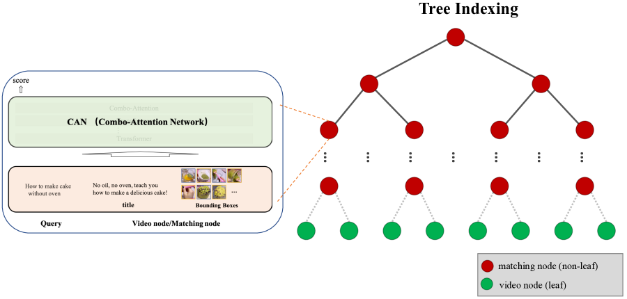
Figure 1: The architecture of the proposed tree-based combo-attention network (TCAN). In the retrieval phase, it only uses CAN to calculate the similarity between the query and the tree node along the traverse path. Since the number of traversed nodes is significantly smaller than that of all videos in the database, the efficiency is considerably boosted.

Traditionally, the text-to-visual cross-modal retrieval is solved by the joint embedding [12, 16]. It maps the features from different modals into the same feature space and thus their similarity can be directly measured by their Euclidean distance in the joint feature space. In the training phase, it seeks to enlarge the distance between the text and its irrelevant images/videos in the joint feature space, and meanwhile minimize the distance between the text and its relevant images/videos in the joint feature space. One of the amazing properties of the joint embedding is that it generates the global text/visual features, and is well compatible with approximate nearest neighbor (ANN) search techniques such as inverted indexing or graph/tree-based indexing. It is hence quite efficient for large-scale cross-modal retrieval applications.

Nevertheless, the global features used in joint embedding methods might not be able to conduct fine-level matching between words and local regions of an image/video. In many cases, only few words in the query sentence are relevant with some small local regions in the video/video. Therefore, to conduct local matching more effectively, some methods [29] rely on local features. Basically, they represent an image by a set of bounding box features and represent the query sentence as a set of word features. Then the relevance score is determined by the set-to-set matching. Recently, inspired by the breakthrough achieved by BERT in NLP, many vision-based BERT methods [47, 37, 59, 36] have been proposed, and achieve an excellent performance in cross-modal tasks like visual question answering (VQA), image captioning and cross-modal retrieval. In parallel, Baidu has launched a combo-attention network (CAN)  [58] for an effective query-to-video retrieval in dynamic video adverting (DVA) platform. Nevertheless, since the cross-attention mechanism used in CAN takes expensive computation cost, it is impossible to use CAN to compute the similarity between the query and all video ads due to limited computing resource. Thus, previously, we first conducted the coarse-level retrieval through title-based retrieval and deployed CAN in the re-ranking phase for the search efficiency. Nevertheless, in this case, some relevant videos might be filtered out in the title-based retrieval due to their low-quality titles. A more reasonable way is to incorporate the cross-modal attention in the early stage.

Recently, tree model is revisited to speed up the deployment of deep models in the recommendation system. Nevertheless, the query’s feature used in our CAN is a set of discrete local features, and thus cannot be represented as an embedding feature to build a tree as TDM [70, 57]. To tackle this problem, we propose a novel dual-path CAN to make it compatible with tree-based model. Based on it, we build Tree-based Combo-Attention Network (TCAN), which is recently launched in Baidu’s dynamic video advertising platform. It achieves high effectiveness by using the combo-attention network (CAN), and meanwhile achieves high efficiency by exploiting the tree structure which avoids exhaustively comparing with each sample in the database. We visualize the overview of the proposed TCAN in Figure 1. Basically, given a query, it traverses the tree from the root to leafs, the combo-attention network is only computed on nodes along the traverse trace, which avoid exhaustively comparing the query with all videos in the database. Given $N$ reference videos in the database, the tree model decreases the computation complexity from $\mathcal{O}(N)$ to $\mathcal{O}(\mathrm{log}(N))$, making it feasible for online serving. After launching the TCAN, we achieve a $2.26\%$ increase in CTR, and a $2.63\%$ increase in CVR.

In a nutshell, the contributions of this paper are four-fold:

• We upgrade the two-stage deployment of original CAN to a one-stage CAN structure. The one-stage CAN simultaneously considers the video’s title and its visual content.

• We design a dual-path structure for one-stage CAN, which supports feature embedding as well as cross attention simultaneously.

• Based on the proposed dual-path CAN, we built a tree-based CAN. Benefited from the tree structure, it achieves an effective and efficiency cross-modal retrieval.

• We have validated the effectiveness of tree-based CAN in Baidu’s dynamic video advertising platform. The promising results demonstrate its usefulness for large-scale cross-modal retrieval in industrial applications.

II Related Work

We review the related work in four fields: cross-modal retrieval, approximate nearest neighbor search, fast neural network and Baidu’s search ads.

II-A Cross-modal Retrieval

The traditional cross-modal retrieval tasks are tackled by joint embedding  [12, 16]. It maps the images and texts from their original feature space into a joint feature space so that they can be compared directly. They target to learn a mapping function, which maximizes the distance between an irrelevant image-text pair to be large , and meanwhile minimizes the distance between relevant image-text pairs. To learn the mapping function more effectively. VSE++ [10] conducts hard negative sampling, which only penalizes the hardest negative sample in each mini-batch. Since the joint-embedding methods generate global features, it well supports feature indexing and thus is quite suitable for large-scale cross-modal retrieval. On the other hand, the global features cannot model the fine-level matching between words and local regions, and thus it might not be effective to capture relevance between an image and a text sentence.

To more effectively describe the relevance between the image and text, several works [29] rely on local features. To be specific, they represent an image by a set of bounding box features which are extracted by pre-trained object detectors. The detected bounding boxes are the candidate locations of objects in the image. Meanwhile, they represent the sentence by a set of word features. Then the relevance between the image and the text sentence is obtained by set-to-set matching between word features and bounding box features. When conducting the set-to-set matching, the relevant word-box pairs with a large similarity score can be easily identified.

To further improvement the performance of text-vision retrieval methods. Several work  [8, 38, 61] inject the cross-modal context when generating image/text representation. For instance, when computing the sentence representation, m-CNN [38] concatenate the image’s feature with words’ features as the input of the 1D convolution. In parallel, when computing image features, BCN [8] uses text features to guide the generation of image features. Recently, inspired by the triumph achieved by BERT in many natural language processing (NLP) tasks [9], some vision-BERT methods  [47, 37] are proposed, achieving excellent performance in many cross-modal tasks such as visual question answering (VQA), image/video captioning and cross-modal retrieval. Basically, the vision-BERT method can be coarsely grouped into two categories. The methods of the first category adopt a single-stream structure. It treats the bounding box features and word features without bias, and directly concatenate them as the input of the self-attention modules. The methods of the second category adopt a two-stream structure. In the text stream, the words features generate query vectors, and the bounding box features are used to generate value vectors and key vectors. On the other hand, in the vision stream, the bounding box features generate query vectors, and the word features are used to generate value vectors and key vectors. In fact, both single-stream and two-stream vision-BERT methods are computationally costly. Therefore, it is impractical to directly use them to conduct large-scale cross-modal retrieval.

II-B Approximated Nearest Neighbor Search

To boost the search efficiency, many approximated nearest neighbor (ANN) search methods are proposed. The research on ANN dates back to at least the 1970s [14, 15]. Traditionally, ANN search methods mainly include hashing-based methods [25, 7, 32, 53, 45, 33, 52, 31], quantization-based method [26, 19, 65, 1], tree-based method [34, 4, 62, 44], and graph-based method [17, 49, 39, 66]. In recent years, “neural ranking” has also attracted increasingly more attentions [70, 69, 50, 72, 18, 48, 57]. Also, inspired by the success of deep learning, many deep Hashing [35, 71] and deep PQ [5, 60] work are proposed. Basically, them incorporate the Hashing and PQ in a neural network, and trains the Hashing or PQ codes in an end-to-end manner.

Despite Hashing codes and PQ codes can enable the fast computation between the query and each reference item, when the number of reference items in the database is large, the time cost is still costly. To make the retrieval more scalable to large-scale dataset, some non-exhaustive search methods are proposed. Inverted multiple indexing (IMI) [3] is one of the most popular methods for non-exhaustive search. Basically, it partitions the feature space into fine cells through the k-means. It only computes the similarity between the query and the cell centroids. Since the number of centroids is significantly smaller than the number of reference items, the efficiency is considerably boosted. In parallel, K-Dimensional tree [46] is another widely used strategy for avoiding comparing the query with each item exhaustively. It builds a binary search tree to partition the feature space, and formulates the retrieval into a tree traverse problem. Recently, TDM [70] also exploits the tree structure to boost the efficiency of deep models deployed in recommendation system. The core idea is that, it only evaluate the expensive deep models in a small subset of tree nodes and avoids evaluating the deep models on all items in the database.

II-C Fast Neural Network

The heavy computation cost of deep neural network limits its usefulness in online serving or mobile applications. Many studies [20] have shown that, network weights might be redundant and do not convey much information. In some cases [63], some large-scale models tend to memorize the dataset instead of learning some generic capability, suffering from serious over-fitting. To boost the efficiency and suppress over-fitting, recently, many efficient and compact neural network architecture are developed, achieving very promising performance in both effectiveness and efficiency. One of most widely used strategy is training quantized neural networks [6, 42, 40, 55, 64, 23]. For instance, [6, 42] design the binary neural network where the value of weights are chosen from two constants. In parallel, some efficient neural networks [20, 54, 24] are obtained by compressing already-trained neural networks. Inspired by the recent success achieved by knowledge distillation [22], some methods [41, 27] propose to find a more compact student network through knowledge distillation. To be specific, [41] jointly learn the weight quantization and the model distillation. [27] designs a Tiny-BERT by distilling the knowledge from the large-scale BERT model. Following the spirit of Tiny-BERT, in our work, we also exploit the knowledge distillation for model compression.

II-D Baidu’s Search Ads

Baidu Search Ads (a.k.a. “Phoenix Nest”) is one of the most important revenue sources for Baidu [11, 13, 56]. In the search industry, sponsored online advertising produces many billions of dollar revenues for online advertisers. Since around 2017, Baidu Search Ads has been undergoing several major upgrades by incorporating the rapid-growing technologies in near neighbor search, machine learning, and systems. For example, [67] reported new architectures for distributed GPU-based parameter servers which have replaced the MPI-based system for training CTR models. [11] described the widespread use of approximate near neighbor search (ANNS) and maximum inner product search (MIPS) [68, 66] to substantially improve the quality of ads recalls in the early stage of the pipeline of Baidu’s ads system. In recent years, Baidu’s short-form video recommendations [30] and video-based search ads have achieved great progress [58, 59, 57]. In this paper, we introduce the technology for a representative project which has significantly boosted Baidu’s video-based ads revenues.

III Background

III-A Definition

Given a video, we extract key frames from it. For each key frame, bounding boxes are detected by Faster R-CNN. Each detected bounding box denotes the location of a candidate object in the key frame. Note that, the detected bounding boxes normally have overlap with each other, and thus there is significant redundancy among the detected bounding boxes. Therefore, after we obtain all the bounding boxes of all keyframes, we utilize the k-means clustering to group them into $K$ clusters. Then the video’s representation is the set of cluster centroids, $\mathbf{C}=[\mathbf{c}_{1},\cdots,\mathbf{c}_{K}]$. Given a query sentence, we obtain a sequence of word features $\mathbf{W}=[\mathbf{w}_{1},\cdots,\mathbf{w}_{M}]$ through a pretrained word embedding.

III-B Basic Block

The combo attention network takes $\mathcal{W}$ and $\mathcal{C}$ as input. Basically, it concatenates $\mathcal{W}$ and $\mathcal{C}$ into a new sequence:

$$\mathbf{M}_{0}=[\mathbf{c}_{1},\cdots,\mathbf{c}_{K},\mathbf{w}_{1},\cdots,\mathbf{w}_{M}].$$ (1)

It adopts a series of standard self-attention modules to process the combined sequence. To be specific, let denote the input of the $i$-th self-attention module by $\mathbf{M}_{i-1}$ and denote the output of the $i$-th self-attention module by $\mathbf{M}_{i}$. It first computes the query vectors $\mathbf{Q}_{i}=[\mathbf{q}_{i,1},\cdots,\mathbf{q}_{i,M+K}]$, key vectors $\mathbf{K}_{i}=[\mathbf{k}_{i,1},\cdots,\mathbf{k}_{i,M+K}]$ and value vectors $\mathbf{V}_{i}=[\mathbf{v}_{i,1},\cdots,\mathbf{v}_{i,M+K}]$ by

$$\mathbf{V}_{i}=f_{i}(\mathbf{M}_{i}),~{}\mathbf{K}_{i}=g_{i}(\mathbf{M}_{i}),~{}\mathbf{Q}_{i}=h_{i}(\mathbf{M}_{i}),$$ (2)

where

$$f_{i}(\mathbf{M}_{i})=\mathbf{W}_{f_{i}}\mathbf{\mathbf{M}_{i}},~{}~{}g_{i}(\mathbf{M}_{i})=\mathbf{W}_{g_{i}}\mathbf{\mathbf{M}_{i}},~{}~{}h_{i}(\mathbf{M}_{i})=\mathbf{W}_{h_{i}}\mathbf{\mathbf{M}_{i}},$$ (3)

, and $\mathbf{W}_{f_{i}}$, $\mathbf{W}_{g_{i}}$ and $\mathbf{W}_{h_{i}}$ are weight matrices to be learned. In implementation, $f_{i}(\cdot)$, $g_{i}(\cdot)$ and $h_{i}(\cdot)$ are implemented by fully-connected layers with the bias fixed as $0$.

For each query vector, $\mathbf{q}_{i,j}$, the self-attention module computes the matrix-vector product between $\mathbf{q}_{i,j}$ and the key matrix $\mathbf{K}_{i}$ followed by a softmax operation, the soft-attention vector $\mathbf{a}_{i,j}$ is obtained by

$$\mathbf{a}_{i,j}=\mathrm{softmax}(\mathbf{K}_{i}\mathbf{q}_{i,j}^{\top}),$$ (4)

where $\mathrm{softmax}$ is defined as

$$\mathrm{softmax}([x_{1},\cdots,x_{D}])=[\frac{e^{x_{1}}}{\sum_{i=1}^{D}e^{x_{i}}},\cdots,\frac{e^{x_{D}}}{\sum_{i=1}^{D}e^{x_{i}}}].$$ (5)

Then the attended feature vector $\mathbf{f}_{i,j}$ is obtained by a weighted summation over all columns of $\mathbf{V}_{i}$ and the weights are items in $\mathbf{a}_{i,j}$:

$$\mathbf{f}_{i,j}=\mathbf{V}_{i}\mathbf{a}_{i,j}^{\top}.$$ (6)

The attended feature matrix $\mathbf{F}_{i}$ consists of all attended features:

$$\mathbf{F}_{i}=[\mathbf{f}_{i,1},\cdots,\mathbf{f}_{i,K+M}].$$ (7)

$\mathbf{F}_{i}$ goes through an add$\&$norm layer and generates:

$${\mathbf{M}}_{i}=\mathrm{norm}(\mathbf{F}_{i}+\mathbf{M}_{i-1}),$$ (8)

where $\mathrm{norm}(\cdot)$ denotes the layer normalization [2]. Note that, for easiness of illustration, the above formulation is based on the single head. In implementation, we adopt an $8$-head settings for all attention blocks.

III-C Similarity and Loss Function

Similarity computation. After the processing of $N$ layers of self-attention modules, we generate the self-attended features $\mathbf{M}_{N}=[\mathbf{m}_{N,1},\cdots,\mathbf{m}_{N,K+M}]$. Among them, $[\mathbf{m}_{N,1},\cdots\mathbf{m}_{N,1}]$ correspond to the attended bounding box centroids and $[\mathbf{m}_{N,K+1},\cdots\mathbf{m}_{N,K+M}]$ correspond to the attended word features. We denote by $\mathbf{c}_{N,j}=\mathbf{m}_{N,j}$ as the $j$-th self-attended centroid and denote by $\mathbf{w}_{N,j}=\mathbf{m}_{N,K+j}$ as the $j$-th self-attended word feature.

Soft attention layer $\mathbf{C}_{N}=[\mathbf{c}_{N,i},\cdots,\mathbf{c}_{N,K}]$ as well as $\mathbf{W}_{N}=[\mathbf{w}_{N,1},\cdots,\mathbf{w}_{N,M}]$ as input, and computes a similarity matrix $\mathbf{S}$ by

$$\mathbf{S}={\mathbf{C}_{N}^{\top}}\mathbf{W}_{N}.$$ (9)

For each column of $\mathbf{S}$, $\mathbf{s}_{i}$, we conduct a soft-max operation on it and obtained a new vector:

$$\tilde{\mathbf{s}}_{i}=\mathrm{softmax}({\mathbf{s}}_{i}).$$ (10)

Then a new similarity matrix is obtained through $\tilde{\mathbf{S}}=[\hat{\mathbf{s}}_{1},\cdots,\hat{\mathbf{s}}_{M}]$. The output of soft attention layer is computed by

$$\tilde{\mathbf{W}}_{N}=\mathbf{C}_{N}\tilde{\mathbf{S}}.$$ (11)

The final similarity score is computed by

$$\mathrm{s}=\sum_{i=1}^{M}\langle\tilde{\mathbf{w}}_{N,i},\mathbf{w}_{N,i}\rangle,$$ (12)

where $\tilde{\mathbf{w}}_{N,i}$ denotes the $i$-th column of $\tilde{\mathbf{W}}_{N}$. In the search phase, the obtained similarity score $s$ is used for ranking the videos given a text query. In the training phase, $s$ is used for constructing the training loss.

Training loss. The training is conducted on each mini-batch. Each mini-batch consists of $K$ ground-truth video-sentence pairs $\{(V_{k},S_{k})\}_{k=1}^{K}$. Each video $V_{k}$ in the mini-batch is only relevant with the sentence in its ground-truth sentence-video pair, $S_{k}$, and irrelevant with other sentences. In the training process, we seek to maximize the similarities between relevant sentence-video pairs and minimize the similarities between irrelevant sentence-video pairs. We denote the similarity score of the video $V_{i}$ and the sentence $S_{j}$ by $s(i,j)$, and construct the loss $\mathcal{L}$ by

$$\begin{split}\mathcal{L}&=\sum_{k=1}^{K}\sum_{j\neq k}[m-s(k,k)+s(k,j)]_{+}\\ &+\sum_{k=1}^{K}\sum_{j\neq k}[m-s(k,k)+s(j,k)]_{+},\end{split}$$ (13)

where $[a]_{+}=max(a,0)$ is a clip function, and $m$ is the margin which we set as $0.2$ by default. Based on the definition, the loss $\mathcal{L}$ only penalizes the pairs beyond the margin $m$. To some extent, this kind of settings only penalizes the hard negative samples. Intuitively, the first part of $\mathcal{L}$ in Eq. (13) focuses on the query side, which penalizes the hard negative videos with respect to the query. On the other hand, the second part of $\mathcal{L}$ focuses on the video side, which penalizes the hard negative queries with respect to the video.

III-D Deployment

Since the computational cost of the CAN is expensive, it is not practical to use it to calculate the similarity between the text query and all videos in the database considering the number of videos is large. Therefore, we only deploy the CAN in the re-ranking stage. As shown in Figure 2, given a text query, we first conduct the title-based search to retrieval top M video candidates. Since we use global feature as the title representation, it readily supports graph indexing and thus makes the title-based search very fast. After that, CAN is used to re-rank the candidate $M$ videos based on their similarity scores.

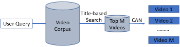
Figure 2: The deployment of CAN in the first launching. Given a query, it first uses the title-based search to recall $M$ candidate videos. After that, it uses CAN to rerank $M$ candidate videos to get the top-K videos. Since the visual information is only considered in the re-ranking phase, some relevant videos might be filtered out in the title-based search phase due to low title quality.

IV Tree-based Combo-Attention Network

As shown in Section III, considering the efficiency issue, CAN was only deployed in the re-ranking phase for high efficiency in the first launching. But this might filter out some relevant videos before re-ranking and limits the effectiveness of CAN. A natural question is raise: can CAN be deployed in the early stage more efficiently? One straightforward solution is to adopt the existing methods for speeding up the neural network to make CAN faster. Nevertheless, in the industrial application, the number of reference in the dataset are normally in the billion scale, making the retrieval even based on a faster CAN still slow.

In the retrieval field, a commonly used strategy to speed up the retrieval is approximated nearest neighbor (ANN) search. By adopting some indexing methods, ANN avoids comparing the query with all reference items in the database, and thus the efficiency is significantly boosted. Nevertheless, the existing architecture of CAN makes it incompatible with indexing-based ANN. On one hand, CAN needs to compute the cross-modal attentions which relies on interactions between the text feature and video feature, making indexing-based ANN search not feasible. On the other hand, CAN relies on discrete local word features and bounding box features, making ANN even harder. In this section, we introduce the tree-based Combo-Attention Network, which simultaneously solves above two obstacles. Basically, the improvement of the proposed TCAN over original CAN is three-fold:

• We simultaneously consider the video’s visual and title information. Thus, we no longer need the two-stage re-ranking process used in previous deployment of CAN. Instead, we can directly obtain the similarity between the query and a video in a single stage.

• We adopt a dual-path structure. On one path, it support the video/query global embedding for the further tree-based video feature indexing. On the other path, it adopts the spirit of original CAN which exploits the cross-modal attention for an effective cross-modal retrieval.

• We build a binary search tree. The tree is constructed by the videos’ embedding. In the search phase, the query is only compared with the nodes along visiting trace, which significantly boosts the efficiency.

• We exploit the knowledge distilling to build a lighter network for faster inference on each tree node.

Below we introduce these four parts in details.

IV-A One-stage CAN

As shown in Figure 2, the first launching of CAN adopts a two-stage method. In the first stage, it only considers the video title and the video’s visual information is considered in the second stage. In contrast, the one-stage CAN simultaneously takes the video’s title and visual content into consideration. The main difference between the original CAN and the current one-stage counterpart lies in the input. We define the query’s word features as $\mathbf{W}_{q}=\{\mathbf{w}_{q,1},\cdots,\mathbf{w}_{q,L}\}$, define the video’s bounding box features as $\mathbf{B}_{v}=\{\mathbf{b}_{v,1},\cdots,\mathbf{b}_{v,M}\}$ and define the video title’s word features as $\mathbf{W}_{v}=\{\mathbf{w}_{v,1},\cdots,\mathbf{w}_{v,M}\}$. The input of the original CAN is $[\mathbf{W}_{q},\mathbf{B}_{v}]$. In contrast, the input of the one-stage CAN is $\mathbf{O}_{0}=[\mathbf{W}_{q},\mathbf{B}_{v},\mathbf{W}_{v}]$. The one-stage CAN also consists of a series of self-attention layers $\{\mathrm{SA}_{t}(\cdot)\}_{t=1}^{T}$. We denote the input of $i$-th SA layer by $\mathbf{O}_{i-1}$ and denote the output of the $i$-th SA layer by $\mathbf{O}_{i}$. In Algorithm 1, we give the detailed process to generate $\mathbf{O}_{i}$ given $\mathbf{O}_{i-1}$.

Algorithm 1 $i$-th self-attention layer in one-stage CAN.

Input:  The input feature $\mathbf{O}_{i-1}$.

Output:  The output feature $\mathbf{O}_{i}$.

1:$\mathbf{Q}_{i}=\mathbf{W}_{f_{i}}\mathbf{\mathbf{M}_{i}}$, $\mathbf{K}_{i}=\mathbf{W}_{g_{i}}\mathbf{\mathbf{M}_{i}}$, $\mathbf{V}_{i}=\mathbf{W}_{h_{i}}\mathbf{\mathbf{M}_{i}}$

2:for $j\in[1,L+M+N]$ do

3:     $\mathbf{q}_{j}\leftarrow\mathbf{Q}_{i}[:,j]$

4:     $\mathbf{a}_{j}\leftarrow\mathrm{softmax}(\mathbf{K}_{i}^{\top}\mathbf{q}_{j})$

5:     $\mathbf{f}_{j}\leftarrow\mathbf{V}_{i}\mathbf{a}_{j}$

6:     $\mathbf{o}_{j}=\mathrm{layernorm}(\mathbf{O}_{i-1}[:,j]+\mathbf{f}_{j})$

7:$\mathbf{O}_{i}=[\mathbf{o}_{1},\cdots,\mathbf{o}_{L+M+N}]$

8:return $\mathbf{O}_{i}$.

Using the output of the last self-attention layer $\mathbf{O}_{N}$, we compute the similarity between the query and the video. The first $L$ elements in $\mathbf{O}_{N}$ correspond to the query’s local features, and the rest elements correspond to the video title’s word features or bounding box features. We define $\mathbf{Q}=\mathbf{O}_{N}[:,0:L]$ as the query’s local features, and define $\mathbf{V}=\mathbf{O}_{N}[:,L:L+M+N]$ as the video’s local feature. Then the similarity between the query and video is calculated by cross-matching between $\mathbf{V}$ and $\mathbf{Q}$. In Algorithm 2, we give the detailed process to generate the cross-matching similarity sim_cross given the query’s local features $\mathbf{Q}$ and the video’s local features $\mathbf{V}$. In the testing phase, the sim_cross determines the traverse trace along the binary search tree which we will introduce later. In the training phase, sim_cross is used for constructing the triplet loss $\mathcal{L}_{cross}$.

Algorithm 2 Cross Matching between the query’s local features $\mathbf{Q}$ and the video’s local features $\mathbf{V}$.

Input:  The query’s local features $\mathbf{Q}$ and the video’s local features $\mathbf{V}$.

Output:  The cross-matching similarity sim_cross.

1:for $j\in[1,L]$ do

2:     $\mathbf{q}_{j}\leftarrow\mathbf{Q}[:,j]$

3:     $\mathbf{a}_{j}\leftarrow\mathrm{softmax}(\mathbf{V}^{\top}\mathbf{q}_{j})$

4:     $\hat{\mathbf{q}}_{j}\leftarrow\mathbf{V}_{i}\mathbf{a}_{j}$

5:sim${}_{\mathrm{cross}}=\sum_{j=1}^{L}\frac{\mathbf{q}_{j}\hat{\mathbf{q}}_{j}}{\|\mathbf{q}_{j}\|_{2}\|\hat{\mathbf{q}}_{j}\|_{2}}$

6:return sim_cross.

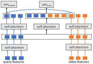
Figure 3: The architecture of dual CAN. It consists of two paths. In the embedding-path, it trains two self-attention modules for the video and query individually, and obtains the video and the query’s embedding feature. The embedding-path is trained by the loss constructed by the embedding similarity sim_embed calculated by the cosine similarity between two embedding features. The obtained videos’ embedding features are further used to construct the binary search tree. In the cross-path, it follows the spirit of the original CAN. It concatenate the video’s local features and the query’s local features, and feed them into a self-attention module to obtain the combo-attention. It is trained by the loss constructed by the cross similarity sim_cross calculated by the soft-attention matching used in the original CAN. In the retrieval phase, sim_cross measures the relevance between the query and nodes of the binary search tree. These two paths share the same early self-attention modules, and are trained jointly.

IV-B Dual-path CAN

Dual-path CAN is extended from CAN. But we make the original CAN a dual-path structure. As visualized in Figure 3, for the first path, it adopts the spirit of the original CAN, the query’s local features and the video’s local features are concatenated and fed into a self-attention module which supplies the combo-attention for an effective cross-modal retrieval. Note that, the video’s local features used in dual CAN not only includes the video’s bounding box features, but also contains the video title’s word features. Meanwhile, it also adopts the same soft-attention similarity measurement as CAN based on local features and generate the cross similarity sim_cross. In the second path, two self-attention modules are trained in parallel. One self-attention module takes input the query’s local features and generate the query’s embedding feature $\mathbf{q}$, the first token’s hidden feature of the last layer. The other self-attention module takes input the video’s local features and generates the video’s global embedding feature $\mathbf{v}$. Then the similarity between the video and the query is obtained by

$$\mathrm{sim}_{\mathrm{embed}}=\langle\mathbf{q},\mathbf{v}\rangle/\|\mathbf{q}\|\|\mathbf{v}\|.$$ (14)

When training the dual-path CAN, we compute a triplet loss $\mathcal{L}_{\mathrm{cross}}$ based on $\mathrm{sim}_{\mathrm{cross}}$ and the other triplet loss $\mathcal{L}_{\mathrm{embed}}$ based on $\mathrm{sim}_{\mathrm{embed}}$. The loss function is obtained by a weighted summation of these two losses:

$$\mathcal{L}_{dual}=\mathcal{L}_{\mathrm{cross}}+\lambda\mathcal{L}_{\mathrm{embed}},$$ (15)

where $\lambda$ is a positive constant which we set as $0.5$ by default. In the search phase, we only use the cross similarity for the tree traverse. On the other hand, we use the video embedding trained from the $\mathcal{L}_{\mathrm{embed}}$ to construct the tree.

IV-C Tree Structure

The binary search tree is constructed based on videos’ embedding feature $\{\mathbf{v}_{1},\cdots,\mathbf{v}_{N}\}$. To be specific, we use hierarchical k-mediods to build the binary search tree based on the clustering results of videos’ embedding feature $\{\mathbf{v}_{1},\cdots,\mathbf{v}_{N}\}$. Note that, there are two ways to conduct the hierarchical k-mediods, the top-down way and the bottom-up way. We use the top-down way considering the efficiency. Meanwhile, we use the industry label of each sample as the initial clustering label for k-mediods. In the tree, the nodes in each layer corresponds to mediods in that level. Meanwhile, we use the node videos’ local features to compute the cross similarity between the query and the node video.

The tree structure and the dual-path CAN are trained in an alternating manner by updating one and fixing the other. To be specific, it conducts two steps alternately. In the first step, for each query, we sample several negative nodes from each layer to train the dual-path CAN model. In the second step, it updates the tree structure based on the videos’ embeding features obtained from the first step. Note that, the negative sampling strategy is quite important for the performance of the proposed tree-based CAN. In Experiment Section, we will compare different negative sampling in details.

Algorithm 3 The tree-based top K retrieval.

Input:    The query’s embedding feature $\mathbf{q}$, the query’s word feature set $\mathcal{W}=\{\mathbf{w}_{1},\cdots,\mathbf{w}_{M}\}$, the number of retrieved videos $K$, the trained tree with depth $L$ and the learned dual-path CAN.

Output:    The top $K$ retrieved videos.

1:Candidate set $\mathcal{C}=\{\mathrm{root}~{}\mathrm{video}~{}\mathrm{node}\}$.

2:for $i\in[1,L]$ do

3:     for $\mathcal{V}\in\mathcal{C}$ do

4:         calculate sim_cross($\mathcal{V},\mathcal{W}$)      

5:     sort $\mathcal{V}\in\mathcal{C}$ in descending order of sim_cross($\mathcal{V},\mathcal{W}$)

6:     get top $K$ video nodes $\mathcal{P}$.

7:     $\mathcal{C}=\{\mathrm{children~{}nodes~{}of}\mathcal{V}|\mathcal{V}\in\mathcal{P}\}$

8:return top $K$ items in $\mathcal{C}$ based on the sim_cross($\mathcal{V},\mathcal{W}$).

Algorithm 3 summarizes the tree-based top K retrieval process. Benefited from the tree structure, the computation complexity of the tree-based top-K retrieval is only $\mathcal{O}(N)$ where $N$ is the number of videos in the database. To be more specific, for a dataset consisting of $10$ million videos, it builds a $23$-layer binary search tree. For each layer, we needs compute sim_cross for two nodes. Thus, in total, we only need visit $1+22\times 2=45$ nodes, i.e., computing $45$ times sim_cross to find the top 1 video.

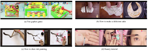
Figure 4: The visualization of query-video pairs. In our Daily1.2B, texts are in Chinese. For the convenience of illustration, we translate the Chinese to English.

IV-D Knowledge Distilling

Considering the heavy computation cost in self-attention layers for evaluating the tree node. We further improves the efficiency through knowledge distilling. We design a student network consists of two self-attention layers with hidden size as $256$ to distill the knowledge from $4$ self-attention layers with hidden size as $768$. The distilling loss is designed in the following way:

$$\mathcal{L}_{distill}=\mathcal{L}_{\mathrm{cross}_{\mathrm{std}}}+\gamma\mathrm{MSE}(\mathrm{sim}_{\mathrm{cross}}-\mathrm{sim}_{\mathrm{cross}_{\mathrm{std}}}),$$ (16)

where $\mathrm{MSE}$ denotes the mean square error, $\mathcal{L}_{\mathrm{cross}_{\mathrm{std}}}$ corresponds to the triplet loss computed based on the cross path of the student network, and $\mathrm{cross}_{\mathrm{std}}$ corresponds to the cross similarity obtained from the student network. $\gamma$ is a constant positive, which we set as $0.3$ by default. The final loss is defined as a weighted summation of $\mathcal{L}_{dual}$ and $\mathcal{L}_{distill}$:

$$\mathcal{L}=\mathcal{L}_{dual}+\beta\mathcal{L}_{distill},$$ (17)

where $\beta$ is a positive constant we set as $0.5$.

V Off-line Experiments

V-A Datasets and Implementation Details

The experiments are conducted on our collected short video dataset, Daily1.2B. It consists of $1.2$ billion pairs of short videos and query sentences, which are mainly about daily lives collected from Baidu’s Haokan APP. Since the relevance between a query and the short videos is relatively subjective to users, we collect ground-truth pairs by selecting the query-video pairs with high click rates, representing good ones for a large number of users. In Figure 4, we visualize some pairs of short videos and query sentences.

For each video, we sample $16$ key frames from each video. For each key frame, $32$ bounding boxes are generated from Faster R-CNN [43] built on ResNet-101 [21] pre-trained on Visual Genomes [28]. For each detected region of the interest (ROI), i.e., the bounding box, its feature is obtained by sum-pooling the convolutional features within the bounding box. The feature dimension is $2048$. We use k-means to group $16\times 32=512$ detected bounding boxes into $32$ clusters and use the cluster centroids as the video’s initial representation. We set the number of head in combo-attention network as $8$. The tree contains 8 million nodes in total, among which, 4 million are leaf nodes. All models are trained and deployed based on the PaddlePaddle deep learning framework developed by Baidu.

V-B One-stage CAN.

Comparisons with two-stage CAN. As we mentioned previously, in the first launching, we conduct a two-stage retrieval process. In this first stage, it exploits title-based search to conduct the coarse-level search and then use CAN for reranking. We compare the proposed one-stage CAN with the two-stage baseline. We vary the number of candidate item pool $M$, among $\{32,64,128,256,512\}$. Two-stage baseline first conduct the title-based search to retrieve the top $20$ items and then conduct re-ranking based on the original CAN. In contrast, our one-stage CAN directly calculate the similarity between the query and $M$ candidate items using the video’s title and visual information. We compare the mAP@3 achieved by ours and that based on two-stage search. As shown in Table I, our one-stage CAN consistently outperforms two-stage CAN.

$M$	$32$	$64$	$128$	$256$	$512$
two-stage	$0.984$	$0.975$	$0.962$	$0.948$	$0.928$
one-stage	$0.993$	$0.989$	$0.980$	$0.971$	$0.950$

TABLE I: mAP@3 comparisons between TCAN with title-based search.

Ablation Study. The one-stage CAN simultaneously considers the video’s title and visual content. We study the influence of each part on the retrieval performance. As shown in Table II, using only video title’s word features, it only achieves a $0.972$ mAP@3. In contrast, using only video’s visual features, the bounding box features, it only achieves a $0.912$ mAP@3. Both of them are lower than mAP@3 achieved by taking both title and visual features into consideration. Meanwhile, despite that there are a large performance gap between the title local features and bounding box visual features, fusing them still achieves a better performance. It demonstrates the effectiveness of self-attention layers in feature fusion.

$M$	$32$	$64$	$128$	$256$	$512$
title	$0.972$	$0.960$	$0.952$	$0.938$	$0.916$
visual	$0.912$	$0.903$	$0.892$	$0.881$	$0.872$
title $\&$ visual	$0.993$	$0.989$	$0.980$	$0.971$	$0.950$

TABLE II: Ablation study on the influence of videos’ titles and visual content on the retrieval performance. The performance is evaluated by mAP@3.

V-C Knowledge Distilling

We conduct the ablation study on knowledge distilling. As mentioned, the original CAN uses $4$ self-attention layers with hidden size as $768$. In contrast, the student network only uses two self-attention layers with hidden size as $256$. As shown in Table III, the performance achieved by the student network is comparable with that of the original CAN, demonstrating the effectiveness of the knowledge distilling. For instance, the original CAN achieves a $0.698$ mAP@1, whereas the student network achieves a $0.694$ mAP@1.

	mAP@
	1	3	5
Original	$0.698$	$0.731$	$0.791$
Student	$0.694$	$0.725$	$0.780$

TABLE III: The ablation study on knowledge distilling.

V-D Comparison with embedding-based binary search tree.

An alternative solution is to use the cosine similarity between query’s embedding and the video’s embedding obtained from the embedding-path to replace the similarity calculated from the CAN when traversing the binary search tree. We compare the TCAN with embedding-based baseline. As shown in Table IV, the proposed TCAN consistently outperforms the embedding-based binary search tree. For instance, our TCAN achieves a $0.694$ mAP@1, whereas mAP@1 of the embedding-based binary search tree is only $0.627$.

	mAP@
	1	3	5
Embed	$0.627$	$0.661$	$0.746$
TCAN	$0.694$	$0.725$	$0.780$

TABLE IV: The comparisons among negative sampling strategies.

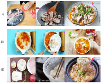
(a) The practice of tomato fish.

(b) How to draw an elephant stick figure.

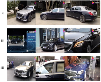
(c) Introduction video of Mercedes-Maybach.

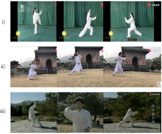
(d) Tai Chi Teaching Video.

Figure 5: Visualization of top-3 retrieved videos. Note that, in our Daily1.2B dataset, the texts are in Chinese.

uniform	arithmetic	geometric
		1.2	1.3	1.4	1.5
$0.713$	$0.821$	$0.860$	$0.895$	$0.966$	$0.965$

TABLE V: The comparisons among negative sampling strategies.

V-E Negative sampling strategy

As we mentioned, when training the dual-path CAN model, we sample negative nodes from each layer of the tree. Since the number of nodes increases exponentially as the depth increases, a general guidance for negative sampling is to sample more negative nodes in deeper layers. We compare different negative sampling strategies including uniform sampling, arithmetic sampling, and geometric sampling. In uniform sampling, we sample the same number of negative nodes for each layer. In arithmetic sampling, we sample $L$ negative samples for the $L$-th level. In geometric sampling, we sample $\lceil L^{\alpha}\rceil$ samples for the $L$-th level. We test the performance of geometric sampling when $\alpha\in\{1.2,1.3,1.4,1.5\}$. The evaluation metric is AUC of the precision-recall retrieval result. As shown in Table V, the negative sampling strategies have significant influence on the retrieval performance. To be specific, the AUC achieved by uniform sampling is only $0.713$, and that achieved by arithmetic sampling is only $0.821$. In contrast, geometric sampling with $\alpha=1.4$ achieves s $0.966$ AUC. By default we adopt geometric sampling with $\alpha=1.4$.

Figure 5 visualizes the retrieval result. For each query, we show three key frames of top3 retrieved videos. As shown in the figure, the retrieval quality is quite high.

VI Online Experiments

We evaluate the proposed TCAN in Baidu dynamic video advertising platform. Two online metrics are used to measure the performance: click-through rate (CTR) and conversion rate (CVR) defined as follows:

$$\mathrm{CTR}=\frac{\#~{}\mathrm{of}~{}\mathrm{clicks}}{\#~{}\mathrm{of}~{}\mathrm{impressions}},\mathrm{CVR}=\frac{\mathrm{revenue}}{\#~{}\mathrm{of}~{}\mathrm{clicks}}.$$ (18)

We compare the CTR and CVR of Baidu dynamic video advertising platform before and after launching the proposed TCAN. Note that, before launching TCAN, the video search is based on title-based retrieval followed by CAN reranking.

metric	CTR	CVR
improvement	$2.29\%$	$2.63\%$

TABLE VI: Online results from May. 17th to May. 20th, 2020 in Baidu dynamic video advertising platform.

As shown in Table VI, after launching TCAN, CTR achieves a $2.29\%$ increase and CVR achieves a $2.63\%$ increase.

VII Conclusion

In this paper, we present the tree-based combo-attention network (TCAN) recently launched in Baidu dynamic video adverting platform. By extending the original CAN to dual-path CAN, it simultaneously supports the cross-modal attention as well as the global feature embedding. Based on the proposed dual-path CAN, we build a binary search tree, which effectively avoid the exhaustive search and significantly boost the retrieval efficiency. The systematic experiments conducted on offline experiments demonstrate its effectiveness for cross-modal retrieval. Meanwhile, the online experiments show the launch of TCAN considerable boosts the revenue of Baidu dynamic video adverting platform.

References

- [1] Fabien André, Anne-Marie Kermarrec, and Nicolas Le Scouarnec. Cache locality is not enough: High-performance nearest neighbor search with product quantization fast scan. volume 9, pages 288–299, 2015.
- [2] Jimmy Lei Ba, Jamie Ryan Kiros, and Geoffrey E Hinton. Layer normalization. arXiv preprint arXiv:1607.06450, 2016.
- [3] Artem Babenko and Victor S. Lempitsky. The inverted multi-index. IEEE Trans. Pattern Anal. Mach. Intell., 37(6):1247–1260, 2015.
- [4] Stefan Berchtold, Daniel A. Keim, and Hans-Peter Kriegel. The x-tree : An index structure for high-dimensional data. In Proceedings of 22th International Conference on Very Large Data Bases (VLDB), pages 28–39, Mumbai (Bombay), India, 1996.
- [5] Yue Cao, Mingsheng Long, Jianmin Wang, Qiang Yang, and Philip S. Yu. Deep visual-semantic hashing for cross-modal retrieval. In Proceedings of the 22nd ACM SIGKDD International Conference on Knowledge Discovery and Data Mining (KDD), pages 1445–1454, San Francisco, CA, 2016.
- [6] Matthieu Courbariaux, Yoshua Bengio, and Jean-Pierre David. Binaryconnect: Training deep neural networks with binary weights during propagations. In Advances in Neural Information Processing Systems (NIPS), pages 3123–3131, Montreal, Quebec, Canada, 2015.
- [7] Mayur Datar, Nicole Immorlica, Piotr Indyk, and Vahab S Mirrokni. Locality-sensitive hashing scheme based on p-stable distributions. In Proceedings of the Twentieth Annual Symposium on Computational Geometry (SCG), pages 253–262, Brooklyn, NY, 2004.
- [8] Harm de Vries, Florian Strub, Jérémie Mary, Hugo Larochelle, Olivier Pietquin, and Aaron C. Courville. Modulating early visual processing by language. In Advances in Neural Information Processing Systems (NIPS), pages 6594–6604, Long Beach, CA, 2017.
- [9] Jacob Devlin, Ming-Wei Chang, Kenton Lee, and Kristina Toutanova. BERT: pre-training of deep bidirectional transformers for language understanding. In Proceedings of the 2019 Conference of the North American Chapter of the Association for Computational Linguistics: Human Language Technologies (NAACL-HLT), pages 4171–4186, Minneapolis, MN, 2019.
- [10] Fartash Faghri, David J. Fleet, Jamie Ryan Kiros, and Sanja Fidler. VSE++: improving visual-semantic embeddings with hard negatives. In Proceedings of British Machine Vision Conference (BMVC), page 12, Newcastle, UK, 2018.
- [11] Miao Fan, Jiacheng Guo, Shuai Zhu, Shuo Miao, Mingming Sun, and Ping Li. MOBIUS: towards the next generation of query-ad matching in baidu’s sponsored search. In Proceedings of the 25th ACM SIGKDD International Conference on Knowledge Discovery & Data Mining (KDD), pages 2509–2517, Anchorage, AK, 2019.
- [12] Ali Farhadi, Seyyed Mohammad Mohsen Hejrati, Mohammad Amin Sadeghi, Peter Young, Cyrus Rashtchian, Julia Hockenmaier, and David A. Forsyth. Every picture tells a story: Generating sentences from images. In Proceedings of the 11th European Conference on Computer Vision (ECCV), Part IV, pages 15–29, Heraklion, Crete, Greece, 2010.
- [13] Hongliang Fei, Jingyuan Zhang, Xingxuan Zhou, Junhao Zhao, Xinyang Qi, and Ping Li. GemNN: Gating-enhanced multi-task neural networks with feature interaction learning for CTR prediction. In Proceedings of the 44th International ACM SIGIR Conference on Research and Development in Information Retrieval (SIGIR), pages 2166–2171, Virtual Event, Canada, 2021.
- [14] Jerome H. Friedman, F. Baskett, and L. Shustek. An algorithm for finding nearest neighbors. IEEE Transactions on Computers, 24:1000–1006, 1975.
- [15] Jerome H. Friedman, J. Bentley, and R. Finkel. An algorithm for finding best matches in logarithmic expected time. ACM Transactions on Mathematical Software, 3:209–226, 1977.
- [16] Andrea Frome, Gregory S. Corrado, Jonathon Shlens, Samy Bengio, Jeffrey Dean, Marc’Aurelio Ranzato, and Tomás Mikolov. Devise: A deep visual-semantic embedding model. In Advances in Neural Information Processing Systems (NIPS), pages 2121–2129, Lake Tahoe, NV, 2013.
- [17] Cong Fu, Chao Xiang, Changxu Wang, and Deng Cai. Fast approximate nearest neighbor search with the navigating spreading-out graph. Proc. VLDB Endow., 12(5):461–474, 2019.
- [18] Weihao Gao, Xiangjun Fan, Chong Wang, Jiankai Sun, Kai Jia, Wenzhi Xiao, Ruofan Ding, Xingyan Bin, Hui Yang, and Xiaobing Liu. Deep retrieval: Learning a retrievable structure for large-scale recommendations. arXiv preprint arXiv:2007.07203, 2020.
- [19] Tiezheng Ge, Kaiming He, Qifa Ke, and Jian Sun. Optimized product quantization for approximate nearest neighbor search. In Proceedings of the IEEE Conference on Computer Vision and Pattern Recognition (CVPR), pages 2946–2953, Portland, OR, 2013.
- [20] Song Han, Huizi Mao, and William J Dally. Deep compression: Compressing deep neural networks with pruning, trained quantization and huffman coding. arXiv preprint arXiv:1510.00149, 2015.
- [21] Kaiming He, Xiangyu Zhang, Shaoqing Ren, and Jian Sun. Deep residual learning for image recognition. In Proceedings of the 2016 IEEE Conference on Computer Vision and Pattern Recognition (CVPR), pages 770–778, Las Vegas, NV, 2016.
- [22] Geoffrey Hinton, Oriol Vinyals, and Jeff Dean. Distilling the knowledge in a neural network. arXiv preprint arXiv:1503.02531, 2015.
- [23] Itay Hubara, Matthieu Courbariaux, Daniel Soudry, Ran El-Yaniv, and Yoshua Bengio. Quantized neural networks: Training neural networks with low precision weights and activations. J. Mach. Learn. Res., 18:187:1–187:30, 2017.
- [24] Forrest N Iandola, Song Han, Matthew W Moskewicz, Khalid Ashraf, William J Dally, and Kurt Keutzer. Squeezenet: Alexnet-level accuracy with 50x fewer parameters and¡ 0.5 mb model size. arXiv preprint arXiv:1602.07360, 2016.
- [25] Piotr Indyk and Rajeev Motwani. Approximate nearest neighbors: Towards removing the curse of dimensionality. In Proceedings of the Thirtieth Annual ACM Symposium on the Theory of Computing (STOC), pages 604–613, Dallas, TX, 1998.
- [26] Hervé Jégou, Matthijs Douze, and Cordelia Schmid. Product quantization for nearest neighbor search. IEEE Trans. Pattern Anal. Mach. Intell., 33(1):117–128, 2011.
- [27] Xiaoqi Jiao, Yichun Yin, Lifeng Shang, Xin Jiang, Xiao Chen, Linlin Li, Fang Wang, and Qun Liu. Tinybert: Distilling BERT for natural language understanding. In Findings of the Association for Computational Linguistics (EMNLP), pages 4163–4174, Online Event, 2020.
- [28] Ranjay Krishna, Yuke Zhu, Oliver Groth, Justin Johnson, Kenji Hata, Joshua Kravitz, Stephanie Chen, Yannis Kalantidis, Li-Jia Li, David A. Shamma, Michael S. Bernstein, and Li Fei-Fei. Visual genome: Connecting language and vision using crowdsourced dense image annotations. Int. J. Comput. Vis., 123(1):32–73, 2017.
- [29] Kuang-Huei Lee, Xi Chen, Gang Hua, Houdong Hu, and Xiaodong He. Stacked cross attention for image-text matching. In Proceedings of the 15th European Conference on Computer Vision (ECCV), Part IV, pages 212–228, Munich Germany, 2018.
- [30] Dingcheng Li, Xu Li, Jun Wang, and Ping Li. Video recommendation with multi-gate mixture of experts soft actor critic. In Proceedings of the 43rd International ACM SIGIR conference on research and development in Information Retrieval (SIGIR), pages 1553–1556, Virtual Event, China, 2020.
- [31] Ping Li. Sign-full random projections. In Proceedings of the Thirty-Third AAAI Conference on Artificial Intelligence (AAAI), pages 4205–4212, Honolulu, HI, 2019.
- [32] Ping Li and Kenneth Ward Church. Using sketches to estimate associations. In Proceedings of the Human Language Technology Conference and the Conference on Empirical Methods in Natural Language Processing (HLT/EMNLP), pages 708–715, Vancouver, Canada, 2005.
- [33] Ping Li, Michael Mitzenmacher, and Anshumali Shrivastava. Coding for random projections. In Proceedings of the 31th International Conference on Machine Learning (ICML), pages 676–684, Beijing, China, 2014.
- [34] King-Ip Lin, H. V. Jagadish, and Christos Faloutsos. The tv-tree: An index structure for high-dimensional data. volume 3, pages 517–542, 1994.
- [35] Venice Erin Liong, Jiwen Lu, Gang Wang, Pierre Moulin, and Jie Zhou. Deep hashing for compact binary codes learning. In Proceedings of the IEEE Conference on Computer Vision and Pattern Recognition (CVPR), pages 2475–2483, Boston, MA, 2015.
- [36] Haoliang Liu, Tan Yu, and Ping Li. Inflate and shrink: Enriching and reducing interactions for fast text-image retrieval. In Proceedings of the 2021 Conference on Empirical Methods in Natural Language Processing (EMNLP), pages 9796–9809, Virtual Event / Punta Cana, Dominican Republic, 2021.
- [37] Jiasen Lu, Dhruv Batra, Devi Parikh, and Stefan Lee. ViLBERT: Pretraining task-agnostic visiolinguistic representations for vision-and-language tasks. In Advances in Neural Information Processing Systems (NeurIPS), pages 13–23, Vancouver, Canada, 2019.
- [38] Lin Ma, Zhengdong Lu, Lifeng Shang, and Hang Li. Multimodal convolutional neural networks for matching image and sentence. In Proceedings of the 2015 IEEE International Conference on Computer Vision (ICCV), pages 2623–2631, Santiago, Chile, 2015.
- [39] Yury A. Malkov and Dmitry A. Yashunin. Efficient and robust approximate nearest neighbor search using hierarchical navigable small world graphs. IEEE Trans. Pattern Anal. Mach. Intell., 42(4):824–836, 2020.
- [40] Joachim Ott, Zhouhan Lin, Ying Zhang, Shih-Chii Liu, and Yoshua Bengio. Recurrent neural networks with limited numerical precision. arXiv preprint arXiv:1608.06902, 2016.
- [41] Antonio Polino, Razvan Pascanu, and Dan Alistarh. Model compression via distillation and quantization. In Proceedings of the 6th International Conference on Learning Representations (ICLR), Vancouver, Canada, 2018.
- [42] Mohammad Rastegari, Vicente Ordonez, Joseph Redmon, and Ali Farhadi. XNOR-Net: Imagenet classification using binary convolutional neural networks. In Proceedings of the 14th European Conference on Computer Vision (ECCV), Part IV, pages 525–542, Amsterdam, The Netherlands, 2016.
- [43] Shaoqing Ren, Kaiming He, Ross B. Girshick, and Jian Sun. Faster R-CNN: towards real-time object detection with region proposal networks. In Advances in Neural Information Processing Systems (NIPS), pages 91–99, Montreal, Canada, 2015.
- [44] Yasushi Sakurai, Masatoshi Yoshikawa, Shunsuke Uemura, and Haruhiko Kojima. The a-tree: An index structure for high-dimensional spaces using relative approximation. In Proceedings of 26th International Conference on Very Large Data Bases (VLDB), pages 516–526, Cairo, Egypt, 2000.
- [45] Anshumali Shrivastava and Ping Li. Fast near neighbor search in high-dimensional binary data. In Proceedings of the European Conference on Machine Learning and Knowledge Discovery in Databases (ECML-PKDD), Part I, pages 474–489, Bristol, UK, 2012.
- [46] Robert F Sproull. Refinements to nearest-neighbor searching ink-dimensional trees. Algorithmica, 6(1-6):579–589, 1991.
- [47] Chen Sun, Austin Myers, Carl Vondrick, Kevin Murphy, and Cordelia Schmid. Videobert: A joint model for video and language representation learning. In Proceedings of the 2019 IEEE/CVF International Conference on Computer Vision (ICCV), pages 7463–7472, Seoul, Korea, 2019.
- [48] Shulong Tan, Weijie Zhao, and Ping Li. Fast neural ranking on bipartite graph indices. Proc. VLDB Endow., 15(4):794–803, 2021.
- [49] Shulong Tan, Zhixin Zhou, Zhaozhuo Xu, and Ping Li. On efficient retrieval of top similarity vectors. In Proceedings of the 2019 Conference on Empirical Methods in Natural Language Processing and the 9th International Joint Conference on Natural Language Processing (EMNLP-IJCNLP), pages 5235–5245, Hong Kong, China, 2019.
- [50] Shulong Tan, Zhixin Zhou, Zhaozhuo Xu, and Ping Li. Fast item ranking under neural network based measures. In Proceedings of the Thirteenth ACM International Conference on Web Search and Data Mining (WSDM), pages 591–599, Houston, TX, 2020.
- [51] Ashish Vaswani, Noam Shazeer, Niki Parmar, Jakob Uszkoreit, Llion Jones, Aidan N Gomez, Łukasz Kaiser, and Illia Polosukhin. Attention is all you need. In Advances in Neural Information Processing Systems (NIPS), pages 5998–6008, Long Beach, CA, 2017.
- [52] Ying Wei, Yangqiu Song, Yi Zhen, Bo Liu, and Qiang Yang. Scalable heterogeneous translated hashing. In Proceedings of the 20th ACM SIGKDD International Conference on Knowledge Discovery and Data Mining (KDD), pages 791–800, New York, NY, 2014.
- [53] Yair Weiss, Antonio Torralba, and Robert Fergus. Spectral hashing. In Advances in Neural Information Processing Systems (NIPS), pages 1753–1760, Vancouver, Canada, 2008.
- [54] Wei Wen, Chunpeng Wu, Yandan Wang, Yiran Chen, and Hai Li. Learning structured sparsity in deep neural networks. In Advances in Neural Information Processing Systems (NIPS), pages 2074–2082, Barcelona, Spain, 2016.
- [55] Xundong Wu, Yong Wu, and Yong Zhao. Binarized neural networks on the imagenet classification task. arXiv preprint arXiv:1604.03058, 2016.
- [56] Zhiqiang Xu, Dong Li, Weijie Zhao, Xing Shen, Tianbo Huang, Xiaoyun Li, and Ping Li. Agile and accurate CTR prediction model training formassive-scale online advertising systems. In Proceedings of the 2021 International Conference on Management of Data (SIGMOD), Online conference [Xi’an, China], 2021.
- [57] Tan Yu, Jie Liu, Yi Yang, Yi Li, Hongliang Fei, and Ping Li. EGM: enhanced graph-based model for large-scale video advertisement search. In Aidong Zhang and Huzefa Rangwala, editors, Proceedings of the 28th ACM SIGKDD Conference on Knowledge Discovery and Data Mining (KDD), pages 4443–4451, Washington, DC, 2022.
- [58] Tan Yu, Yi Yang, Yi Li, Xiaodong Chen, Mingming Sun, and Ping Li. Combo-attention network for baidu video advertising. In Proceedings of the 26th ACM SIGKDD Conference on Knowledge Discovery and Data Mining (KDD), pages 2474–2482, Virtual Event, CA, USA, 2020.
- [59] Tan Yu, Yi Yang, Yi Li, Lin Liu, Mingming Sun, and Ping Li. Multi-modal dictionary BERT for cross-modal video search in baidu advertising. In Proceedings of the 30th ACM International Conference on Information and Knowledge Management (CIKM), pages 4341–4351, Virtual Event, Queensland, Australia, 2021.
- [60] Tan Yu, Junsong Yuan, Chen Fang, and Hailin Jin. Product quantization network for fast image retrieval. In Proceedings of the 15th European Conference on Computer Vision (ECCV), Part I, pages 191–206, Munich, Germany, 2018.
- [61] Youngjae Yu, Hyungjin Ko, Jongwook Choi, and Gunhee Kim. End-to-end concept word detection for video captioning, retrieval, and question answering. In Proceedings of the 2017 IEEE Conference on Computer Vision and Pattern Recognition (CVPR), pages 3261–3269, Honolulu, HI, 2017.
- [62] Pavel Zezula, Pasquale Savino, Giuseppe Amato, and Fausto Rabitti. Approximate similarity retrieval with m-trees. volume 7, pages 275–293, 1998.
- [63] Chiyuan Zhang, Samy Bengio, Moritz Hardt, Benjamin Recht, and Oriol Vinyals. Understanding deep learning requires rethinking generalization. In Proceedings of the 5th International Conference on Learning Representations (ICLR), Toulon, France, 2017.
- [64] Hantian Zhang, Jerry Li, Kaan Kara, Dan Alistarh, Ji Liu, and Ce Zhang. ZipML: Training linear models with end-to-end low precision, and a little bit of deep learning. In Proceedings of the 34th International Conference on Machine Learning (ICML), pages 4035–4043, Sydney, Australia, 2017.
- [65] Ting Zhang, Chao Du, and Jingdong Wang. Composite quantization for approximate nearest neighbor search. In Proceedings of the 31th International Conference on Machine Learning (ICML), pages 838–846, Beijing, China, 2014.
- [66] Weijie Zhao, Shulong Tan, and Ping Li. SONG: approximate nearest neighbor search on GPU. In Proceedings of the 36th IEEE International Conference on Data Engineering (ICDE), pages 1033–1044, Dallas, TX, 2020.
- [67] Weijie Zhao, Jingyuan Zhang, Deping Xie, Yulei Qian, Ronglai Jia, and Ping Li. AIBox: CTR prediction model training on a single node. In Proceedings of the 28th ACM International Conference on Information and Knowledge Management (CIKM), pages 319–328, Beijing, China, 2019.
- [68] Zhixin Zhou, Shulong Tan, Zhaozhuo Xu, and Ping Li. Möbius transformation for fast inner product search on graph. In Advances in Neural Information Processing Systems (NeurIPS), pages 8216–8227, Vancouver, Canada, 2019.
- [69] Han Zhu, Daqing Chang, Ziru Xu, Pengye Zhang, Xiang Li, Jie He, Han Li, Jian Xu, and Kun Gai. Joint optimization of tree-based index and deep model for recommender systems. In Advances in Neural Information Processing Systems (NeurIPS), pages 3973–3982, Vancouver, Canada, 2019.
- [70] Han Zhu, Xiang Li, Pengye Zhang, Guozheng Li, Jie He, Han Li, and Kun Gai. Learning tree-based deep model for recommender systems. In Proceedings of the 24th ACM SIGKDD International Conference on Knowledge Discovery & Data Mining (KDD), pages 1079–1088, London, UK, 2018.
- [71] Han Zhu, Mingsheng Long, Jianmin Wang, and Yue Cao. Deep hashing network for efficient similarity retrieval. In Proceedings of the Thirtieth AAAI Conference on Artificial Intelligence (AAAI), pages 2415–2421, Phoenix, AZ, 2016.
- [72] Jingwei Zhuo, Ziru Xu, Wei Dai, Han Zhu, Han Li, Jian Xu, and Kun Gai. Learning optimal tree models under beam search. In Proceedings of the 37th International Conference on Machine Learning (ICML), pages 11650–11659, Virtual Event, 2020.