Impact of Anisotropic Birefringence on Measuring Cosmic Microwave Background Lensing

Abstract

The power spectrum of cosmic microwave background lensing is a powerful tool for constraining fundamental physics such as the sum of neutrino masses and the dark energy equation of state. Current lensing measurements primarily come from distortions to the microwave background temperature field, but the polarization lensing signal will dominate upcoming experiments with greater sensitivity. Cosmic birefringence refers to the rotation of the linear polarization direction of microwave photons propagating from the last scattering surface to us, which can be induced by parity-violating physics such as axion-like dark matter or primordial magnetic fields. We find that, for an upcoming CMB-S4-like experiment, scale-invariant anisotropic birefringence with an amplitude corresponding to the current $95\%$ upper bound can bias the measured lensing power spectrum by up to a factor of a few at small scales, $L\gtrsim 1000$. We show that the bias scales linearly with the amplitude of the scale-invariant birefringence spectrum. The signal-to-noise of the contribution from anisotropic birefringence is larger than unity even if the birefringence amplitude decreases to around $5\%$ of the current upper bound. Our results indicate that measurement and characterization of possible anisotropic birefringence is important for lensing analysis in future low-noise polarization experiments.

I Introduction

Cosmic microwave background (CMB) lensing refers to the deflection of CMB photons by the matter distribution along their path from the last scattering surface to the observer. This effect creates a displacement field on the microwave sky, causing subtle distortions in both the CMB temperature and polarization maps. This displacement leads to correlations of CMB temperature and polarization fluctuations on a wide range of angular scales, which can be used to reconstruct the lensing displacement field Hu and Okamoto (2002); Okamoto and Hu (2003). Precise measurements of CMB lensing probes the matter distribution of the universe and places constraints on cosmological parameters such as the amplitude of matter density fluctuations, $\sigma_{8}$, and the energy density of matter, $\omega_{m}$, to which CMB lensing is particularly sensitive.

CMB lensing has been measured with increasing significance by several experiments, including Planck Planck Collaboration et al. (2020, 2014); Carron et al. (2022), ACT van Engelen et al. (2015), BICEP BICEP2 Collaboration et al. (2016), Polarbear Polarbear Collaboration et al. (2014); POLARBEAR Collaboration et al. (2017), and SPT van Engelen et al. (2012); Story et al. (2015), and will be measured with higher precision in the upcoming experiments like Simons Observatory Ade et al. (2019) and CMB-S4 Abazajian et al. (2016). To date, lensing detection from temperature maps dominates the signal-to-noise for all of these experiments. As map noise levels decrease, CMB polarization maps are eventually expected to provide higher signal-to-noise in upcoming surveys such as CMB-S4 Abazajian et al. (2016).

Compared to temperature lensing, polarization lensing is much less affected by various contaminants such as the thermal and kinematic Sunyaev–Zeldovich (tSZ, kSZ) effects, which may significantly bias temperature-based lensing reconstruction Ferraro and Hill (2018); Cai et al. (2022) at arcminute angular scales. However, polarization-based lensing reconstruction can also be biased by effects such as instrumental systematics Mirmelstein et al. (2021); Nagata and Namikawa (2021). Another potential bias comes from cosmic birefringence, which refers to a rotation of CMB linear polarization plane caused by some parity-violating physics such as primordial magnetic fields or axion-like particles. Cosmic birefringence can potentially be isotropic, with a constant rotation independent of direction on the sky, or a direction-dependent anisotropic rotation. Several recent analyses of Planck polarization data find a tantalizing hint of isotropic birefringence Minami and Komatsu (2020); Diego-Palazuelos et al. (2022); Eskilt and Komatsu (2022). Cosmic birefringence therefore has gained growing interest; for a recent review see, e.g., Komatsu (2022)). Anticipating such a discovery, multiple recent papers have explored the potential of future CMB experiments to constrain the mass of axion-like particles Sherwin and Namikawa (2021); Nakatsuka et al. (2022); Lee et al. (2022); Gasparotto and Obata (2022) and to probe models which produce both isotropic and anisotropic cosmic birefringence Capparelli et al. (2020); Fujita et al. (2020); Kitajima et al. (2022); Jain et al. (2022).

To leading order, an anisotropic rotation field induced by cosmic birefringence does not bias the reconstructed lensing field, thanks to the orthogonality between the lensing and rotation response in the CMB polarization field Kamionkowski (2009). However, an anisotropic rotation field may potentially bias the reconstructed lensing power spectrum, a possibility which has not previously been considered in detail. In this paper we examine such a bias in the presence of a scale-invariant rotation field.

The paper is structured as follows. In Sec. II we summarize the basics of CMB lensing and cosmic birefringence. In Sec. III we review CMB lensing reconstruction on full-sky using the EB estimator and explain the motivation for investigating the bias to the reconstructed CMB lensing power spectrum. Sec. IV presents simulation procedures and numerical results. We discuss the results in Sec. V and conclude in Sec. VI.

II Lensed and Rotated CMB Power Spectra

Both CMB lensing and anisotropic cosmic birefringence affect the CMB polarization field in a similar way. In this section we first give an overview of their effects on the CMB polarization field in II.1, followed by brief reviews of CMB lensing and cosmic birefringence in II.2 and II.3, respectively. We then summarize some relevant results about power spectra in II.4.

II.1 Overview

Linear polarization of the CMB can be described by the Stokes parameters $Q(\bm{\hat{n}})$ and $U(\bm{\hat{n}})$, measured with respect to a set of local orthogonal polarizers, with $\bm{\hat{n}}$ an angular coordinate on the sky. The sky direction dependence of $Q$ and $U$ can be decomposed into spin-weighted spherical harmonics Goldberg et al. (1967) to obtain rotation-invariant quantities $E$ and $B$ as Kamionkowski et al. (1997); Zaldarriaga and Seljak (1997)

$$E_{\ell m}\pm iB_{\ell m}=-\int d^{2}\bm{\hat{n}}~{}{}_{\pm 2}Y^{*}_{\ell m}(Q\pm iU)(\bm{\hat{n}}),$$ (1)

with $E_{\ell m}$ and $B_{\ell m}$ the multipole moments of E-mode and B-mode polarization, respectively. Their power spectra are defined as

$$\langle E_{\ell m}E^{*}_{\ell^{\prime}m^{\prime}}\rangle=\delta_{\ell\ell^{\prime}}\delta_{mm^{\prime}}C^{\mathrm{EE}}_{\ell}$$ (2)

$$\langle B_{\ell m}B^{*}_{\ell^{\prime}m^{\prime}}\rangle=\delta_{\ell\ell^{\prime}}\delta_{mm^{\prime}}C^{\mathrm{BB}}_{\ell}$$

$$\langle E_{\ell m}B^{*}_{\ell^{\prime}m^{\prime}}\rangle=\delta_{\ell\ell^{\prime}}\delta_{mm^{\prime}}C^{\mathrm{EB}}_{\ell},$$

where the $\langle...\rangle$ is taken over different statistical realizations of the CMB. The primary CMB polarization fields have no off-diagonal covariance between different $\ell$ and $m$ values.

The effects of both CMB lensing and cosmic birefringence can be interpreted as small perturbations added to the primary CMB field, effected by the lensing potential, $\phi(\bm{\hat{n}})$, for CMB lensing, and a rotation field, $\alpha(\bm{\hat{n}})$, for cosmic birefringence. In the presence of both CMB lensing and cosmic birefringence, the CMB polarization fields can be described as

$$\tilde{E}^{\prime}_{\ell m} = E_{\ell m}+\delta\tilde{E}_{\ell m}+\delta E^{\prime}_{\ell m}+\mathcal{O}(\phi^{n_{1}}\alpha^{n_{2}}),$$ (3)

$$\tilde{B}^{\prime}_{\ell m} = \delta\tilde{B}_{\ell m}+\delta B^{\prime}_{\ell m}+\mathcal{O}(\phi^{n_{1}}\alpha^{n_{2}}),$$ (4)

where $\delta\tilde{E}_{\ell m}$, $\delta\tilde{B}_{\ell m}$ denote the first-order perturbation from CMB lensing, $\delta E^{\prime}_{\ell m}$, $\delta B^{\prime}_{\ell m}$ denote that from the rotation field, and $\mathcal{O}(\phi^{n_{1}}\alpha^{n_{2}})$, with $n_{1}+n_{2}>1$, represents the higher-order terms which mix the lensing and rotation effects. In the subsequent subsections we will discuss each of the terms in detail.

II.2 CMB lensing

CMB lensing distortion occurs when photons are deflected by gravitational potentials and measures the integrated mass distribution along the trajectories of photons (for a review, see, e.g. Lewis and Challinor (2006)). Lensing distortion results in an effective displacement field $\bm{d}(\bm{\hat{n}})$ acting on the primary CMB fields,

$$\begin{split}\tilde{T}(\bm{\hat{n}})&=T(\bm{\hat{n}}+\bm{d}(\bm{\hat{n}})),\\ (\tilde{Q}\pm i\tilde{U})(\bm{\hat{n}})&=(Q\pm iU)(\bm{\hat{n}}+\bm{d}(\bm{\hat{n}})).\end{split}$$ (5)

Under Born’s approximation and the assumption that all CMB photons come from the last scattering surface, and neglecting non-linear effects, the displacement field $\bm{d}(\bm{\hat{n}})$ can be expressed as a pure gradient,

$$\bm{d}(\bm{\hat{n}})=\nabla\phi(\bm{\hat{n}}),$$ (6)

with $\phi(\bm{\hat{n}})$ the lensing potential field given by

$$\phi(\bm{\hat{n}})=-2\int_{0}^{\chi_{\ast}}d\chi\frac{\chi_{\ast}-\chi}{\chi_{\ast}\chi}\Psi(\chi\bm{\hat{n}},\eta_{0}-\chi)$$ (7)

in a flat universe, with $\chi_{\ast}$ the conformal distance to the last scattering surface, $\eta_{0}$ the conformal time today, and $\Psi$ the (Weyl) gravitational potential.

One can similarly decompose the lensing potential field in spherical harmonics as

$$\phi(\hat{\mathbf{n}})=\sum_{LM}\phi_{LM}Y_{LM}(\hat{\mathbf{n}}),$$ (8)

with the multipole moments $\phi_{LM}$ related to its power spectrum as

$$\left\langle\phi_{LM}\phi_{L^{\prime}M^{\prime}}^{*}\right\rangle=\delta_{LL^{\prime}}\delta_{MM^{\prime}}C_{L}^{\phi\phi}.$$ (9)

Using the Limber approximation, the power spectrum $C_{L}^{\phi\phi}$ can be expressed as

$$C_{L}^{\phi\phi}\approx\frac{8\pi^{2}}{L^{3}}\int_{0}^{\chi_{\ast}}\chi d\chi\left(\frac{\chi_{\ast}-\chi}{\chi_{\ast}\chi}\right)^{2}P_{\Psi}\left(\frac{L}{\chi};\eta_{0}-\chi\right).$$ (10)

Here $P_{\Psi}(k;\eta)$ is the power spectrum of the gravitational potential, which is connected to the matter power spectrum $P_{m}(k;\eta)$ by

$$P_{\Psi}(k;\eta)=\frac{9\Omega^{2}_{m}(\eta)H^{4}(\eta)}{8\pi^{2}}\frac{P_{m}(k;\eta)}{k},$$ (11)

with $\Omega_{m}(\eta)$ the fractional matter energy density and $H(\eta)$ the Hubble parameter at conformal time $\eta$. Hence, CMB lensing encodes information about the matter distribution, especially at late times (as the integrand in Eq. (10) peaks at $z\approx 2$). Measuring CMB lensing therefore constrains cosmological parameters such as the matter fluctuation amplitude $\sigma_{8}$, the matter density $\Omega_{\mathrm{m}}$, the spatial curvature of the universe $\Omega_{k}$, the sum of neutrino masses $\sum m_{\nu}$, and the dark energy equation of state $w$, as previously demonstrated in, e.g., Sherwin et al. (2017); van Engelen et al. (2012).

A promising way to measure CMB lensing is through its effect on CMB polarization field Hu and Okamoto (2002); Okamoto and Hu (2003). Following from Eq. (5), CMB lensing leads to perturbations in CMB E-mode and B-mode polarization fields, given by

$$\delta\tilde{E}_{\ell m}=\sum_{LM}\sum_{\ell^{\prime}m^{\prime}}(-1)^{m}\phi_{LM} \left(\begin{array}[]{ccc}\ell&L&\ell^{\prime}\\ -m&M&m^{\prime}\end{array}\right)$$ (12)

$$\times{}_{2}F^{\mathrm{\phi}}_{\ell L\ell^{\prime}}\epsilon_{\ell L\ell^{\prime}}E_{\ell^{\prime}m^{\prime}}$$

and

$$\delta\tilde{B}_{\ell m}=\sum_{LM}\sum_{\ell^{\prime}m^{\prime}}(-1)^{m}\phi_{LM} \left(\begin{array}[]{ccc}\ell&L&\ell^{\prime}\\ -m&M&m^{\prime}\end{array}\right)$$ (13)

$$\times{}_{2}F^{\phi}_{\ell L\ell^{\prime}}\beta_{\ell L\ell^{\prime}}E_{\ell^{\prime}m^{\prime}}$$

to leading order in $\phi$, where $\epsilon_{\ell L\ell^{\prime}}$ and $\beta_{\ell L\ell^{\prime}}$ are parity terms defined as

$$\epsilon_{\ell L\ell^{\prime}}\equiv\frac{1+(-1)^{\ell+L+\ell^{\prime}}}{2},$$ (14)

$$\beta_{\ell L\ell^{\prime}}\equiv\frac{1-(-1)^{\ell+L+\ell^{\prime}}}{2i},$$

and the function ${}_{2}F^{\phi}_{\ell L\ell^{\prime}}$ is defined as

$$~{}{}_{2}F^{\phi}_{\ell L\ell^{\prime}}\equiv \left[-\ell\left(\ell+1\right)+L(L+1)+\ell^{\prime}\left(\ell^{\prime}+1\right)\right]$$ (15)

$$\times \sqrt{\frac{\left(2\ell+1\right)(2L+1)\left(2\ell^{\prime}+1\right)}{16\pi}}\left(\begin{array}[]{ccc}\ell&L&\ell^{\prime}\\ 2&0&-2\end{array}\right).$$

The perturbation to the CMB polarization fields introduces off-diagonal covariance in and between E-mode and B-mode polarization fields and therefore allows measuring the lensing potential by optimally weighting quadratic combinations of the CMB polarization fields (known as the quadratic estimator approach) Okamoto and Hu (2003). In the next part we will see that rotations of the CMB polarization field have similar effects.

II.3 Cosmic Birefringence

In addition to the lensing distortion, CMB linear polarization may also undergo rotation in propagating from the last scattering surface to us. This phenomenon is called cosmic birefringence. Cosmic birefringence can be caused by parity-violating physics in the early universe, such as axion-like particles coupling to photons through Chern-Simons interaction Carroll (1998); Li and Zhang (2008); Marsh (2016), more general Lorentz-violating physics beyond the Standard Model Leon et al. (2016), and primordial magnetic fields through frequency-dependent Faraday rotation Kosowsky and Loeb (1996); Harari et al. (1997); Kosowsky et al. (2005); Yadav et al. (2012); De et al. (2013); Pogosian (2014). The rotated linear polarization field can be expressed as

$$(Q^{\prime}\pm iU^{\prime})(\bm{\hat{n}})=e^{\pm 2i\alpha(\bm{\hat{n}})}(Q\pm iU)(\bm{\hat{n}}),$$ (16)

with $\alpha(\bm{\hat{n}})$ the rotation field. We use primes to represent the rotated quantities.

As a specific example, cosmic birefringence is induced by a Chern-Simons-type interaction between photons and axion-like particles in the early universe with a Lagrangian given by

$$\mathcal{L}_{cs}=\frac{g_{a\gamma}a}{4}F^{\mu\nu}\tilde{F}_{\mu\nu},$$ (17)

where $g_{a\gamma}$ is a dimensionless coupling constant, $a$ is the axion field, and $F^{\mu\nu}$ is the electromagnetic tensor with $\tilde{F}_{\mu\nu}$ being its dual. This term modifies the Euler-Lagrange equations for the electromagnetic field and induces a rotation in the polarization direction of a photon if $a$ varies along its propagation path Colladay and Kostelecký (1997, 1998); Leon et al. (2017), with the rotation angle given by

$$\alpha(\hat{\bm{n}})=\frac{g_{a\gamma}}{2}\Delta a,$$ (18)

where $\Delta a$ is the change of $a$ along the photon path from the last scattering surface to us.

A generic rotation field can be separated into an isotropic constant piece $\bar{\alpha}$ and an anisotropic part $\delta\alpha(\hat{\bm{n}})$ as

$$\alpha(\hat{\bm{n}})=\bar{\alpha}+\delta\alpha(\hat{\bm{n}})$$ (19)

with

$$\langle\delta\alpha(\hat{\bm{n}})\rangle=0.$$ (20)

For example, some quintessence models predict both isotropic and anisotropic cosmic birefringence Caldwell et al. (2011), while some massless scalar fields do not necessarily induce isotropic cosmic birefringence Gluscevic et al. (2009). Isotropic cosmic birefringence violates global parity symmetry and induces odd-parity CMB TB and EB power spectra, but does not produce any correlations between CMB polarization fields at different angular scales.

In the subsequent analysis we consider only anisotropic cosmic birefringence with $\bar{\alpha}=0$, as it behaves similarly to CMB lensing which is also anisotropic. Similar to Eq. (8), we can decompose the rotation field into multipole moments using spherical harmonics as

$$\alpha(\hat{\mathbf{n}})=\sum_{LM}\alpha_{LM}Y_{LM}(\hat{\mathbf{n}}),$$ (21)

and the rotation field power spectrum is given by

$$\left\langle\alpha_{LM}\alpha_{L^{\prime}M^{\prime}}^{*}\right\rangle=\delta_{LL^{\prime}}\delta_{MM^{\prime}}C_{L}^{\alpha\alpha}.$$ (22)

Anisotropies in the rotation field can result from inhomogeneities in the axion field, for example. If the axion field is seeded during inflation, it leads to a Gaussian random rotation field with a nearly scale-invariant spectrum at large scales ($L\lesssim 100$), with an amplitude connected to the inflationary Hubble parameter $H_{\mathrm{I}}$:

$$\frac{L(L+1)C_{L}^{\alpha\alpha}}{2\pi}=\left(\frac{H_{\mathrm{I}}g_{a\gamma}}{4\pi}\right)^{2}\equiv A_{\mathrm{CB}},$$ (23)

where we have defined a dimensionless amplitude $A_{\rm CB}$ of the scale-invariant rotation power spectrum. Current best constraints on $A_{\rm CB}$ are given by ACTPol Namikawa et al. (2020) and SPTPol Bianchini et al. (2020) corresponding to a $2\sigma$ upper bound $A_{\mathrm{CB}}\leq 10^{-5}$. With improved sensitivity in the next-generation ground-based CMB experiments, we expect the constraint of $A_{\rm CB}$ to reach the level of $10^{-7}$ Aiola et al. (2022); Pogosian et al. (2019); Mandal et al. (2022).

In this paper we focus only on scale-invariant rotation field for conceptual simplicity, but the methodology is generally applicable to rotation field with any power spectrum. We expect the conclusion from other rotational power spectra to be qualitatively similar, but we leave a detailed quantitative analysis of such cases to future work.

Similar to CMB lensing in Eq. (12), a rotation field leads to perturbations in the CMB E-mode and B-mode polarization fields given by Kamionkowski (2009); Gluscevic et al. (2009)

$$\delta E^{\prime}_{\ell m}=-2\sum_{LM}\sum_{\ell^{\prime}m^{\prime}}(-1)^{m}\alpha_{LM} \left(\begin{array}[]{ccc}\ell&L&\ell^{\prime}\\ -m&M&m^{\prime}\end{array}\right)$$ (24)

$$\times{}_{2}F^{\alpha}_{\ell L\ell^{\prime}}\beta_{\ell L\ell^{\prime}}E_{\ell^{\prime}m^{\prime}},$$

$$\delta B^{\prime}_{\ell m}=2\sum_{LM}\sum_{\ell^{\prime}m^{\prime}}(-1)^{m}\alpha_{LM} \left(\begin{array}[]{ccc}\ell&L&\ell^{\prime}\\ -m&M&m^{\prime}\end{array}\right)$$ (25)

$$\times{}_{2}F^{\alpha}_{\ell L\ell^{\prime}}\epsilon_{\ell L\ell^{\prime}}E_{\ell^{\prime}m^{\prime}},$$

to leading order in $\alpha$ from Eq. (16), where we have assumed that $C_{l}^{\rm BB}$ is negligible before rotation. $\beta_{\ell L\ell^{\prime}}$ and $\epsilon_{\ell L\ell^{\prime}}$ are defined in Eq. (14), and ${}_{2}F^{\alpha}_{\ell L\ell^{\prime}}$ is defined as

$${}_{2}F^{\alpha}_{\ell L\ell^{\prime}}\equiv\sqrt{\frac{\left(2\ell+1\right)(2L+1)\left(2\ell^{\prime}+1\right)}{4\pi}}\left(\begin{array}[]{ccc}\ell&L&\ell^{\prime}\\ 2&0&-2\end{array}\right).$$ (26)

Note that the parity indicators in Eq. (24) and Eq. (25) are opposite to the ones in Eq. (12) and Eq. (13), i.e., $\delta\tilde{E}$ and $\delta B^{\prime}_{\ell m}$ are only non-zero when $\ell+L+\ell^{\prime}$ is even and $\delta\tilde{B}$ and $\delta E^{\prime}_{\ell m}$ are only non-zero when $\ell+L+\ell^{\prime}$ is odd. In this sense, we say that CMB lensing and anisotropic cosmic birefringence are orthogonal at leading order Kamionkowski (2009).

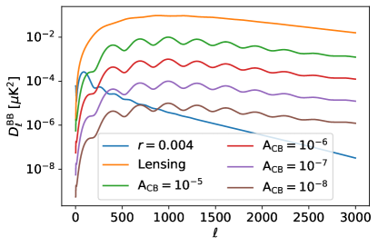
Figure 1: B-mode power spectrum contributions from a scale-invariant tensor mode ($r=0.004$), gravitational lensing, and 1st-order scale-invariant anisotropic birefringence with different amplitudes ($A_{\mathrm{CB}}=10^{-5}$, $A_{\mathrm{CB}}=10^{-6}$, $A_{\mathrm{CB}}=10^{-7}$ and $A_{\mathrm{CB}}=10^{-8}$) are shown, where we define $D^{BB}_{\ell}\equiv\ell(\ell+1)C_{\ell}^{BB}/2\pi$. All the power spectra shown above are generated by class_rot Cai and Guan (2022).

II.4 Summary remarks

Both CMB lensing and anisotropic cosmic birefringence lead to perturbations in the CMB E-mode and B-mode polarization fields. The resulting B-mode power spectrum reveals their relative contributions. In Fig. 1, we compare the B-mode power spectrum from a scale-invariant primordial tensor mode with $r=0.004$, gravitational lensing, and scale-invariant anisotropic rotation fields with different amplitudes ($A_{\mathrm{CB}}=10^{-5}$, $A_{\mathrm{CB}}=10^{-6}$, $A_{\mathrm{CB}}=10^{-7}$, and $A_{\mathrm{CB}}=10^{-8}$). Like CMB lensing, scale-invariant anisotropic rotation contributes predominantly to small-scale anisotropies in B-mode polarization, with a power spectrum generally orders of magnitude below the CMB lensing signal for observationally allowed amplitudes.

In addition to contributing to the CMB polarization power spectra, both CMB lensing and rotation lead to off-diagonal covariance between E-mode and B-mode polarization fields Gluscevic et al. (2009),

$${\langle E_{\ell m}\delta\tilde{B}_{\ell^{\prime}m^{\prime}}\rangle}_{\mathrm{CMB}} =\sum_{LM}\begin{pmatrix}\ell&\ell^{\prime}&L\\ m&m^{\prime}&M\end{pmatrix}f^{\phi}_{\ell L\ell^{\prime}}\phi^{*}_{LM},$$ (27)

$$\langle E_{\ell m}\delta B^{\prime}_{\ell^{\prime}m^{\prime}}\rangle_{\mathrm{CMB}} =\sum_{LM}\begin{pmatrix}\ell&\ell^{\prime}&L\\ m&m^{\prime}&M\end{pmatrix}f^{\alpha}_{\ell L\ell^{\prime}}\alpha^{*}_{LM},$$

for $\ell\neq\ell^{\prime}$ and $m\neq-m^{\prime}$. $f^{\phi}_{\ell L\ell^{\prime}}$ and $f^{\alpha}_{\ell L\ell^{\prime}}$ are weight functions for $\phi$ and $\alpha$, given by

$$f^{\phi}_{\ell L\ell^{\prime}} =-\beta_{\ell L\ell^{\prime}}~{}{}_{2}F^{\phi}_{\ell L\ell^{\prime}}C^{\mathrm{EE}}_{\ell},$$ (28)

$$f^{\alpha}_{\ell L\ell^{\prime}} =-2\epsilon_{\ell L\ell^{\prime}}~{}{}_{2}F^{\alpha}_{\ell L\ell^{\prime}}C^{\mathrm{EE}}_{\ell}.$$

Here $\langle...\rangle_{\mathrm{CMB}}$ is an ensemble average over different realizations of the primary CMB, with a fixed realization of both $\phi$ and $\alpha$. It then follows that

$$\langle\tilde{E}^{\prime}_{\ell m}\tilde{B}^{\prime}_{\ell^{\prime}m^{\prime}}\rangle_{\mathrm{CMB}}= \sum_{LM}\begin{pmatrix}\ell&\ell^{\prime}&L\\ m&m^{\prime}&M\end{pmatrix}f^{\phi}_{\ell L\ell^{\prime}}\phi^{*}_{LM}$$ (29)

$$+ \sum_{LM}\begin{pmatrix}\ell&\ell^{\prime}&L\\ m&m^{\prime}&M\end{pmatrix}f^{\alpha}_{\ell L\ell^{\prime}}\alpha^{*}_{LM},$$

for $\ell\neq\ell^{\prime}$ and $m\neq-m^{\prime}$. Eq. (29) shows that the off-diagonal covariance between E-mode and B-mode polarization is contributed by a sum of lensing and rotation contributions, to leading order.

III CMB Lensing reconstruction bias due to a rotation field

In this section, we introduce the CMB lensing reconstruction pipeline considered in this work. In particular, we focus on the EB estimator, as it is expected to be a dominant source of statistical power for lensing reconstruction in upcoming experiments Okamoto and Hu (2003). We then discuss the motivation and our methodology for evaluating the bias to the estimated lensing power spectrum from a rotation field.

III.1 Lensing reconstruction

The lensing potential can be reconstructed from the off-diagonal covariance generated by CMB lensing in Eq. (29) using a quadratic estimator approach. An estimator for lensed E and B maps is given by Okamoto and Hu (2003)

$$\hat{\phi}_{LM}=A_{L}\sum_{\ell m}\sum_{\ell^{\prime}m^{\prime}}(-1)^{M} \left(\begin{array}[]{ccc}\ell&\ell^{\prime}&L\\ m&m^{\prime}&-M\end{array}\right)$$ (30)

$$\times(f^{\phi}_{\ell L\ell^{\prime}})^{*}\frac{\tilde{E}_{\ell m}}{\hat{C}^{\mathrm{EE}}_{\ell}}\frac{\tilde{B}_{\ell^{\prime}m^{\prime}}}{\hat{C}^{\mathrm{BB}}_{\ell^{\prime}}},$$

where $A_{L}$ is a normalization factor ensuring $\hat{\phi}_{LM}$ is unbiased, given by

$$A_{L}=\left(\frac{1}{2L+1}\sum_{\ell\ell^{\prime}}\frac{|f^{\phi}_{\ell L\ell^{\prime}}|^{2}}{\hat{C}^{\mathrm{EE}}_{\ell}\hat{C}^{\mathrm{BB}}_{\ell^{\prime}}}\right)^{-1},$$ (31)

and $\hat{C}^{\mathrm{EE}}_{\ell}$ and $\hat{C}^{\mathrm{BB}}_{\ell}$ are the total observed EE and BB power spectra with noise power spectrum included. The quadratic estimator $\hat{\phi}_{LM}$ collects all the off-diagonal correlations of a CMB map realization and average them by a weight function $f^{\phi}_{\ell L\ell^{\prime}}$.

From the reconstructed lensing potential, its power spectrum can be estimated as Sherwin et al. (2017)

$$\hat{C}_{L}^{\phi\phi}=C_{L}^{\hat{\phi}\hat{\phi}}-{}^{(\mathrm{RD})}N^{(0)}_{L}-N^{(1)}_{L}-N^{(\mathrm{MC})}_{L}-N^{(\mathrm{FG})}_{L},$$ (32)

with $C_{L}^{\hat{\phi}\hat{\phi}}$ given by

$$C_{L}^{\hat{\phi}\hat{\phi}}=\frac{1}{2L+1}\sum_{M=-L}^{L}\left|\hat{\phi}_{LM}\right|^{2}.$$ (33)

The remaining terms in Eq. (33) are noise biases that need to be subtracted: ${}^{(\mathrm{RD})}N^{(0)}_{L}$ is the realization-dependent Gaussian noise (RDN0) Namikawa et al. (2013) (Appendix A discusses the motivation to use this instead of the standard Gaussian noise $N^{(0)}_{L}$). $N^{(1)}_{L}$ represents the bias from connected terms in the CMB four-point function which contain the first-order lensing potential $C^{\phi\phi}_{L}$. $N^{(\mathrm{MC})}_{L}$ is the “Monte-Carlo”(MC) noise encapsulating biases not accounted for otherwise, such as higher-order reconstruction noise estimated from MC simulations, and $N^{(\mathrm{FG})}_{L}$ is the modeled foreground bias from extragalactic and galactic foregrounds like galactic dust, galaxy clusters and the cosmic infrared background.

III.2 Bias to $C_{L}^{\phi\phi}$ from rotation

Now consider a scenario in which we perform lensing reconstruction on a set of polarization maps which have been unknowingly rotated: how will this affect our estimated $C_{L}^{\phi\phi}$? To understand this, we can define an effective estimator

$$\hat{\phi^{\prime}}_{LM}=A_{L}\sum_{\ell m}\sum_{\ell^{\prime}m^{\prime}}(-1)^{M} \left(\begin{array}[]{ccc}\ell&\ell^{\prime}&L\\ m&m^{\prime}&-M\end{array}\right)$$ (34)

$$\times(f^{\phi}_{\ell L\ell^{\prime}})^{*}\frac{\tilde{E}^{\prime}_{\ell m}}{\hat{C}^{\mathrm{EE}}_{\ell}}\frac{\tilde{B}^{\prime}_{\ell^{\prime}m^{\prime}}}{\hat{C}^{\mathrm{BB}}_{\ell^{\prime}}},$$

which uses the rotated-lensed quantities $\tilde{E}^{\prime}_{\ell m}$, $\tilde{B}^{\prime}_{\ell m}$ in place of the lensed-only ones.

This estimator does not bias the reconstructed lensing potential, up to leading order in $\phi$ and $\alpha$ (also see Appendix B of Gluscevic et al. (2009) for a similar discussion). This can be demonstrated by taking the ensemble average of $\hat{\phi}^{\prime}_{LM}$ over different CMB realizations,

$$\langle\hat{\phi}^{\prime}_{LM}\rangle_{\mathrm{CMB}}= A_{L}\sum_{\ell m}\sum_{\ell^{\prime}m^{\prime}}\sum_{L^{\prime}M^{\prime}}(-1)^{M}$$ (35)

$$\times\left(\begin{array}[]{ccc}\ell&\ell^{\prime}&L\\ m&m^{\prime}&-M\end{array}\right)\begin{pmatrix}\ell&\ell^{\prime}&L^{\prime}\\ m&m^{\prime}&M^{\prime}\end{pmatrix}$$

$$\times\left((f^{\phi}_{\ell L\ell^{\prime}})^{*}f^{\phi}_{\ell L^{\prime}\ell^{\prime}}\phi^{*}_{L^{\prime}M^{\prime}}+(f^{\phi}_{\ell L\ell^{\prime}})^{*}f^{\alpha}_{\ell L^{\prime}\ell^{\prime}}\alpha^{*}_{L^{\prime}M^{\prime}}\right).$$

Applying the orthogonality relation of the Wigner-3j symbols,

$$\sum_{mm^{\prime}}\left(\begin{array}[]{ccc}\ell&\ell^{\prime}&L\\ m&m^{\prime}&-M\end{array}\right)\begin{pmatrix}\ell&\ell^{\prime}&L^{\prime}\\ m&m^{\prime}&M^{\prime}\end{pmatrix}=\frac{1}{2L+1}\delta_{LL^{\prime}}\delta_{M,-M^{\prime}},$$ (36)

and the orthogonality of the parity indicators

$$\epsilon_{\ell L\ell^{\prime}}\beta_{\ell L\ell^{\prime}}=0,$$ (37)

we can see that the leading-order rotation contribution disappears due to parity, and we get

$$\langle\hat{\phi}^{\prime}_{LM}\rangle_{\mathrm{CMB}} =A_{L}\sum_{\ell\ell^{\prime}}\frac{1}{2L+1}\frac{|f^{\phi}_{\ell L\ell^{\prime}}|^{2}}{\hat{C}^{\mathrm{EE}}_{\ell}\hat{C}^{\mathrm{BB}}_{\ell^{\prime}}}\phi_{LM}$$ (38)

$$=\phi_{LM},$$

which shows that our estimator for the lensing potential $\phi$ remains unbiased.

However, we should emphasize that an unbiased $\phi$ does not necessarily imply an unbiased $C_{L}^{\phi\phi}$. Similar to the fact that $\langle x\rangle=0$ does not imply $\langle x^{2}\rangle=0$, the estimator, $C_{L}^{\hat{\phi}\hat{\phi}}$ contains quadratic terms in $\hat{\phi}$ and thus may be biased. In addition, higher-order terms in Eq. (24) and Eq. (25) may also break the orthogonality between CMB lensing and anisotropic rotation and induce bias to $\hat{C}_{L}^{\phi\phi}$.

Based on Eq. (32), we define the bias from rotation to the reconstructed CMB lensing power spectrum as

$$\Delta(\hat{C}_{L}^{\phi\phi})_{\mathrm{rot}}\equiv\langle\hat{C^{\prime}}_{L}^{\phi\phi}\rangle-\langle\hat{C}_{L}^{\phi\phi}\rangle$$ (39)

where $\langle...\rangle$ represents the average over the reconstructed lensing power spectra from different realizations of the sky, and $\hat{C^{\prime}}_{L}^{\phi\phi}$ refers to applying the power spectrum estimator given in Eq. (32) to rotated-lensed CMB maps.

Among the noise biases in Eq. (32), we assume that anisotropic rotation does not affect $N^{(1)}_{L}$, $N^{(\mathrm{MC})}_{L}$ and $N^{(\mathrm{FG})}_{L}$ on full sky. RDN0, on the other hand, is calculated based on the observed CMB power spectrum and therefore will be affected by rotation as it changes the CMB polarization power spectra (as shown in Fig. 1). RDN0 is calculated based on both “data” and MC simulation, encapsulating all the disconnected terms in the CMB four-point correlation Namikawa et al. (2013); Madhavacheril et al. (2020). Consequently, when compared with a standard MC $\mathrm{N}^{(0)}_{L}$, RDN0 automatically mitigates the biases from small changes to the CMB covariance, such as that arising from rotation in the context of this paper. See Appendix. A for further details.

We can then write Eq. (39) as

$$\Delta(\hat{C}_{L}^{\phi\phi})_{\mathrm{rot}}= \langle C^{\hat{\phi^{\prime}}\hat{\phi^{\prime}}}_{L}\rangle-\langle C^{\hat{\phi}\hat{\phi}}_{L}\rangle$$ (40)

$$- (\langle{}^{(\mathrm{RD})}\mathrm{N}^{\prime(0)}_{L}\rangle-\langle{}^{(\mathrm{RD})}\mathrm{N}^{(0)}_{L}\rangle),$$

where $\langle\hat{C}^{\prime\mathrm{\phi}\mathrm{\phi}}_{L}\rangle$ and $\langle\hat{C}^{\mathrm{\phi}\mathrm{\phi}}_{L}\rangle$ represent the average over the two sets of reconstructed lensing potential power spectra using rotated lensed and unrotated lensed CMB maps respectively, and $\langle{}^{(\mathrm{RD})}\mathrm{N}^{\prime(0)}_{L}\rangle$ and $\langle{}^{(\mathrm{RD})}\mathrm{N}^{(0)}_{L}\rangle$ represent the corresponding average RDN0. We will show the computation of RDN0 in the following Section.

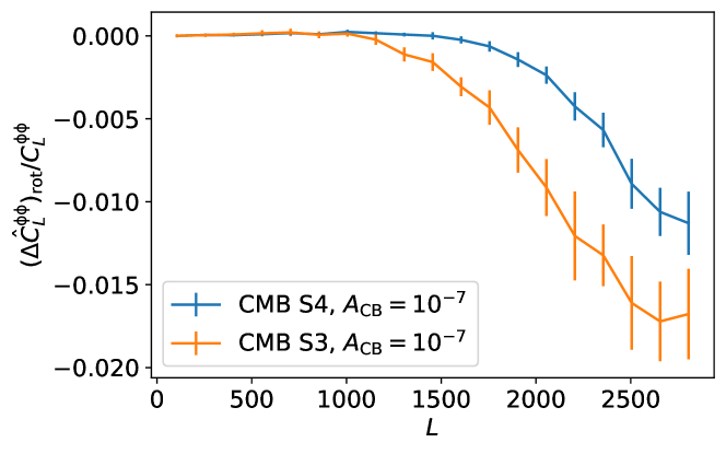
Figure 2: The fractional bias of the reconstructed lensing potential power spectrum from a scale-invariant anisotropic rotation field with amplitude $A_{\mathrm{CB}}=10^{-7}$ for a CMB-S3-like experiment and a CMB-S4-like experiment. We apply full-sky CMB lensing reconstruction using the EB estimator, for the CMB multipole range from $\ell_{\mathrm{min}}=30$ to $\ell_{\mathrm{max}}=3000$. The curves are binned by $\Delta\ell=150$, and the error bars on $\Delta(\hat{C}_{L}^{\phi\phi})_{\mathrm{rot}}$ are estimated from the scatter among the differences of the reconstructed CMB lensing power spectra using rotated-lensed CMB polarization realizations and using lensed CMB polarization realizations.

IV Simulation and Results

As discussed in Sec. III, to estimate the bias $\Delta(\hat{C}_{L}^{\phi\phi})_{\mathrm{rot}}$ in Eq. (40), we need two sets of simulated CMB polarization maps: one set with both CMB lensing and rotation, and the other set with CMB lensing only. The first set of simulations is generated by rotating the lensed simulations in pixel space with a random realization of rotation field. All simulations in this work are generated in CAR pixelization on the full sky using pixell Naess et al. (2021). We then use cmblensplus to perform the CMB lensing reconstruction on the full sky which avoids unnecessary complications due to partial sky coverage. Below we summarize our simulation steps:

1. We generate 10 realizations of lensed CMB polarization maps {$\tilde{X}(\hat{\bm{n}})$} ($X\in\{E,B\}$) as our mock data, based on a fiducial power spectrum that does not include the cosmic birefringence effect, $C_{l}^{XX}|_{\rm fid}$, given by the best-fit cosmology from Planck 2018 Planck Collaboration et al. (2018).

2. We generate 10 Gaussian realizations of an anisotropic rotation field, {$\alpha(\hat{\bm{n}})$}, assuming a scale-invariant power spectrum with $A_{\mathrm{CB}}=10^{-7}$ as defined in Eq. (23), which corresponds to a $1\sigma$ upper limit for CMB-S3-like experiments Pogosian et al. (2019). This amplitude corresponds to an rms rotation of around 0.05 degrees.

3. We perform a pixel-wise polarization rotation on each $\tilde{X}(\bm{\hat{n}})$ with the rotation field $\alpha(\hat{\bm{n}})$ to make a set of 10 rotated-lensed CMB polarization maps, denoted as {$\tilde{X}^{\prime}(\bm{\hat{n}})$}. Both $\{\tilde{X}(\bm{\hat{n}})\}$ and $\{\tilde{X}^{\prime}(\bm{\hat{n}})\}$ are used as mock data.

4. We perform full-sky CMB lensing reconstruction using cmblensplus Namikawa (2021) on both sets of mock data, {$\tilde{X}(\bm{\hat{n}})$} and {$\tilde{X}^{\prime}(\bm{\hat{n}})$}, and obtain an average lensing power spectrum for each set of simulations, denoted as $\langle C^{\hat{\mathrm{\phi}}\hat{\mathrm{\phi}}}_{L}\rangle$ and $\langle C^{\hat{\mathrm{\phi^{\prime}}}\hat{\mathrm{\phi^{\prime}}}}_{L}\rangle$. We restrict lensing reconstruction to multipoles between $\ell_{\mathrm{min}}=30$ to $\ell_{\mathrm{max}}=3000$. We use the Knox formula for including detector noise in the power spectrum Knox (1995),

   $$\hat{C}_{\ell}^{XX}=C_{\ell}^{XX}|_{\rm fid}+N_{\ell},$$ (41)

   with the homogeneous detector noise power spectrum for polarization given by

   $$N_{\ell}=\Delta^{2}_{\mathrm{P}}e^{\ell(\ell+1)\theta^{2}_{\mathrm{FWHM}}/(8\ln 2)},$$ (42)

   where $\Delta_{\mathrm{P}}$ is the polarization noise level of the experiment and $\theta_{\mathrm{FWHM}}$ is the full-width at half maximum (FWHM) of the beam in radians. Note that although experimental noise is modeled at the power spectrum level in $\hat{C}_{l}^{XX}$, Gaussian noise in the map does not affect the estimation of lensing bias but introduces additional scatter in the result, so we choose not to include it in our simulated maps.

5. Following Namikawa et al. (2013); Madhavacheril et al. (2020), we calculate RDN0 for each map in $\{\tilde{X}\}$ and $\{\tilde{X}^{\prime}\}$ by making two additional set of lensed CMB simulations, $\{\tilde{X}^{S_{1}}\}$ and $\{\tilde{X}^{S_{2}}_{i}\}$, based on the fiducial model without cosmic birefringence as in step 1, each containing 20 simulations. These two sets of independent realizations, $\{\tilde{X}^{S_{1}}\}$ and $\{\tilde{X}^{S_{2}}_{i}\}$, are needed in calculating RDN0 as a way to minimize errors from statistical uncertainties in covariance matrix estimation or mismodeling (see Appendix A for a more detailed discussion). For a given map, $\tilde{X}(\bm{\hat{n}})$, we calculate its RDN0 as

   $${}^{(\mathrm{RD})}\mathrm{N}^{(0)}_{L}= \langle C_{L}^{\hat{\phi}\hat{\phi}}[\tilde{E}\tilde{B}^{S_{1}},\tilde{E}\tilde{B}^{S_{1}}]+C_{L}^{\hat{\phi}\hat{\phi}}[\tilde{E}^{S_{1}}\tilde{B},\tilde{E}\tilde{B}^{S_{1}}]$$ (43)

   $$+C_{L}^{\hat{\phi}\hat{\phi}}[\tilde{E}^{S_{1}}\tilde{B},\tilde{E}^{S_{1}}\tilde{B}]+C_{L}^{\hat{\phi}\hat{\phi}}[\tilde{E}\tilde{B}^{S_{1}},\tilde{E}^{S_{1}}\tilde{B}]$$

   $$-C_{L}^{\hat{\phi}\hat{\phi}}[\tilde{E}^{S_{1}}\tilde{B}^{S_{2}},\tilde{E}^{S_{1}}\tilde{B}^{S_{2}}]$$

   $$-C_{L}^{\hat{\phi}\hat{\phi}}[\tilde{E}^{S_{1}}\tilde{B}^{S_{2}},\tilde{E}^{S_{2}}\tilde{B}^{S_{1}}]\rangle_{S_{1},S_{2}},$$

   and similarly we calculate RDN0 for a given rotated-lensed map $\tilde{X}^{\prime}$ as

   $${}^{(\mathrm{RD})}\mathrm{N}^{\prime(0)}_{L}= \langle C_{L}^{\hat{\phi}\hat{\phi}}[\tilde{E}^{\prime}\tilde{B}^{S_{1}},\tilde{E}^{\prime}\tilde{B}^{S_{1}}]+C_{L}^{\hat{\phi}\hat{\phi}}[\tilde{E}^{S_{1}}\tilde{B}^{\prime},\tilde{E}^{\prime}\tilde{B}^{S_{1}}]$$ (44)

   $$+C_{L}^{\hat{\phi}\hat{\phi}}[\tilde{E}^{S_{1}}\tilde{B}^{\prime},\tilde{E}^{S_{1}}\tilde{B}^{\prime}]+C_{L}^{\hat{\phi}\hat{\phi}}[\tilde{E}^{\prime}\tilde{B}^{S_{1}},\tilde{E}^{S_{1}}\tilde{B}^{\prime}]$$

   $$-C_{L}^{\hat{\phi}\hat{\phi}}[\tilde{E}^{S_{1}}\tilde{B}^{S_{2}},\tilde{E}^{S_{1}}\tilde{B}^{S_{2}}]$$

   $$-C_{L}^{\hat{\phi}\hat{\phi}}[\tilde{E}^{S_{1}}\tilde{B}^{S_{2}},\tilde{E}^{S_{2}}\tilde{B}^{S_{1}}]\rangle_{S_{1},S_{2}},$$

   where the combinations in $\left[...\right]$ represent the input maps for lensing reconstruction, and $\langle...\rangle_{S_{1},S_{2}}$ refers to an average over the two sets of MC simulations ($S_{1}$, $S_{2}$) . Using Eq. (43) and (44), we calculate RDN0 for each simulation in $\{\tilde{X}(\bm{\hat{n}})\}$ and $\{\tilde{X}^{\prime}(\bm{\hat{n}})\}$ and calculate the average within each set of simulations, denoted as $\langle{}^{(\mathrm{RD})}\mathrm{N}^{(0)}_{L}\rangle$ and $\langle{}^{(\mathrm{RD})}\mathrm{N}^{\prime(0)}_{L}\rangle$ respectively. Note that, as mentioned in the last step, simulated CMB maps in Eq. (43) and (44) do not contain map noise, so the calculated RDN0 only contains contribution from cosmic variance.

6. We then estimate the lensing bias, $\Delta(\hat{C}_{L}^{\phi\phi})_{\mathrm{rot}}$ using Eq. (40), and calculate fractional bias defined as $\Delta(\hat{C}_{L}^{\phi\phi})_{\mathrm{rot}}/C^{\phi\phi}_{L}$, with $C^{\phi\phi}_{L}$ the power spectrum of the CMB lensing potential from the fiducial model.

7. We repeat the above procedures for two sets of experimental configurations: CMB-S3-like and CMB-S4-like. The experimental configurations including the noise level and beam size are list in Table 1.

In Fig. 2, we show the fractional bias, $\Delta(\hat{C}_{L}^{\phi\phi})_{\mathrm{rot}}/C^{\phi\phi}_{L}$, obtained from the procedure described above for both CMB-S3-like and CMB-S4-like experiments. We find that a rotation field with $A_{\mathrm{CB}}=10^{-7}$, which is well below the current experimental constraint, is capable of introducing a percent-level bias to the reconstructed lensing power spectrum. The bias is most evident at small scales ($L\gtrsim 1000$), reaching up to $1.5\%$ for CMB-S3-like experiments and slightly lower for CMB-S4-like experiments.

The signal-to-noise ratio (SNR) of the contribution from the anisotropic birefringence is

$${\rm SNR}=\left(\sum_{L}\frac{f_{\rm sky}L\left(\Delta(\hat{C}_{L}^{\phi\phi})_{\mathrm{rot}}\right)^{2}}{\left(C_{L}^{\phi\phi}+N^{(0)}_{L}\right)^{2}}\right)^{1/2},$$ (45)

where $N^{(0)}$ is calculated theoretically using cmblensplus that contains contributions from both cosmic variance and map noise, and $f_{\rm sky}=0.4$, accounting for the partial sky coverage of a ground-based experiment. Using Eq. (45), we estimate that the contribution of cosmic birefringence with $A_{\rm CB}=10^{-7}$ has a SNR of $0.2$ for a CMB-S4-like experiment.

Expt	${\Delta}_{T}~{}[\mathrm{\mu K^{\prime}}]$	${\theta}_{\mathrm{FWHM}}[^{\prime}]$
CMB-S3-like	7	1.4
CMB-S4-like	1	1.4

Table 1: Experiments configurations considered in this study.

V The Source of Bias

To understand the observed bias, we compare the four-point correlation function contained in $C_{L}^{\hat{\phi}^{\prime}\hat{\phi}^{\prime}}$,

$$\langle\tilde{E}^{\prime}_{\ell_{1}m_{1}}\tilde{B}^{\prime}_{\ell_{2}m_{2}}\tilde{E}^{\prime}_{\ell_{3}m_{3}}\tilde{B}^{\prime}_{\ell_{4}m_{4}}\rangle,$$ (46)

to the four-point correlation function in $C_{L}^{\hat{\phi}\hat{\phi}}$,

$$\langle\tilde{E}_{\ell_{1}m_{1}}\tilde{B}_{\ell_{2}m_{2}}\tilde{E}_{\ell_{3}m_{3}}\tilde{B}_{\ell_{4}m_{4}}\rangle.$$ (47)

To leading order, a dominant contribution to their difference is given by

$$\begin{split}&\>\>\>\>\>\>\langle E_{\ell_{1}m_{1}}\delta B^{\prime}_{\ell_{2}m_{2}}E_{\ell_{3}m_{3}}\delta B^{\prime}_{\ell_{4}m_{4}}\rangle\\ &\propto\langle E_{\ell_{1}m_{1}}(E_{\ell^{\prime}_{2}m^{\prime}_{2}}\alpha_{LM})E_{\ell_{3}m_{3}}(E_{\ell^{\prime}_{4}m^{\prime}_{4}}\alpha_{L^{\prime}M^{\prime}})\rangle,\end{split}$$ (48)

where we have applied Eq. (25) and used parentheses to indicate useful groupings of terms. As we have assumed $\alpha$ to be a Gaussian random field, Eq. (LABEL:eq:bias_main_term) can be simplified using Wick’s theorem into products of two-point correlation functions that fall into two classes: disconnected terms and connected terms.

A disconnected term can be expressed as

$${\contraction{\langle}{E}{{}_{\ell_{1}m_{1}}(E_{\ell^{\prime}_{2}m^{\prime}_{2}}\alpha_{LM})}{E}\contraction[2ex]{\langle E_{\ell_{1}m_{1}}(}{E}{{}_{\ell^{\prime}_{2}m^{\prime}_{2}}\alpha_{LM})E_{\ell_{3}m_{3}}(}{E}\bcontraction{\langle E_{\ell_{1}m_{1}}(E_{\ell^{\prime}_{2}m^{\prime}_{2}}}{\alpha}{{}_{LM})E_{\ell_{3}m_{3}}(E_{\ell^{\prime}_{4}m^{\prime}_{4}}}{\alpha}\langle E_{\ell_{1}m_{1}}(E_{\ell^{\prime}_{2}m^{\prime}_{2}}\alpha_{LM})E_{\ell_{3}m_{3}}(E_{\ell^{\prime}_{4}m^{\prime}_{4}}\alpha_{L^{\prime}M^{\prime}})\rangle},$$ (49)

where we have used Wick contraction notation to denote products of two-point correlation functions. This term is classified as a disconnected term of the CMB four-point correlation function, because fields within the same “group”, e.g., $E_{\ell^{\prime}_{2}m’_{2}}$ and $\alpha_{LM}$ (as indicated by the parentheses), follow the same contraction behaviour, i.e., contracting with a common group, $E_{\ell^{\prime}_{4}m^{\prime}_{4}}$ and $\alpha_{L^{\prime}M^{\prime}}$. If, on the other hand, contraction behavior of fields in the same group is different, we classify the term as connected. For example, the term

$${\contraction{\langle}{E}{{}_{\ell_{1}m_{1}}(E_{\ell^{\prime}_{2}m^{\prime}_{2}}\alpha_{LM})E_{\ell_{3}m_{3}}(}{E}\contraction[2ex]{\langle E_{\ell_{1}m_{1}}(}{E}{{}_{\ell^{\prime}_{2}m^{\prime}_{2}}\alpha_{LM})}{E}\bcontraction{\langle E_{\ell_{1}m_{1}}(E_{\ell^{\prime}_{2}m^{\prime}_{2}}}{\alpha}{{}_{LM})E_{\ell_{3}m_{3}}(E_{\ell^{\prime}_{4}m^{\prime}_{4}}}{\alpha}\langle E_{\ell_{1}m_{1}}(E_{\ell^{\prime}_{2}m^{\prime}_{2}}\alpha_{LM})E_{\ell_{3}m_{3}}(E_{\ell^{\prime}_{4}m^{\prime}_{4}}\alpha_{L^{\prime}M^{\prime}})\rangle},$$ (50)

is connected, and so is

$${\contraction{\langle}{E}{{}_{\ell_{1}m_{1}(}}{E}\contraction{\langle E_{\ell_{1}m_{1}}({E}{{}_{\ell^{\prime}_{2}m^{\prime}_{2}}\alpha_{LM})}}{E}{{}_{\ell_{3}m_{3}}(}{E}\bcontraction{\langle E_{\ell_{1}m_{1}}(E_{\ell^{\prime}_{2}m^{\prime}_{2}}}{\alpha}{{}_{LM})E_{\ell_{3}m_{3}}(E_{\ell^{\prime}_{4}m^{\prime}_{4}}}{\alpha}\langle E_{\ell_{1}m_{1}}(E_{\ell^{\prime}_{2}m^{\prime}_{2}}\alpha_{LM})E_{\ell_{3}m_{3}}(E_{\ell^{\prime}_{4}m^{\prime}_{4}}\alpha_{L^{\prime}M^{\prime}})\rangle}.$$ (51)

In both cases $E_{\ell^{\prime}_{2}m^{\prime}_{2}}$ and $\alpha_{LM}$ do not contract with a common group. The distinction of disconnected and connected terms is important because the RDN0 technique that we apply mitigates the leading-order biases in the disconnected terms of the four-point correlation, such as that in Eq. (49), but cannot mitigate biases in the connected terms. Hence we expect that a dominant contribution to the observed bias in Sec. IV comes from the accumulated effect of all connected terms, such as Eq. (50) and (51).

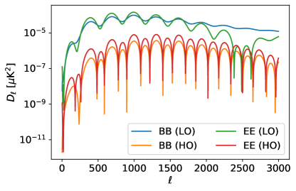
Figure 3: B-mode power spectrum contributions from the leading-order (LO) contribution and higher-order (HO) contribution of scale-invariant anisotropic cosmic birefringence with an amplitude of $A_{\mathrm{CB}}=10^{-7}$. The former is about two order of magnitude larger than the latter. The power spectra shown here are generated by class_rot Cai and Guan (2022).

In the above discussion we have neglected the effect of higher-order terms which mix lensing and rotation. Higher-order terms break the orthogonality between lensing and rotation, leading to bias in $\hat{\phi}$; they also contribute additional connected terms to $\hat{C}_{l}^{\phi\phi}$. In Fig. 3 we show the contributions from leading-order and higher-order terms to the power spectrum, calculated using class_rot. We find that for $A_{\rm CB}=10^{-7}$, higher-order terms generally contribute a few percent of the leading-order power spectrum bias.

If the contributions from connected terms, such as Eq. (50) and (51), are dominant and the higher-order terms can be neglected, we expect the size of the observed bias to scale linearly with $C_{L}^{\alpha\alpha}$ and thus linearly with $A_{\rm CB}$. To verify this, we repeat the steps in Sec. IV for $A_{\rm CB}=10^{-6}$ and $10^{-8}$ and compare the resulting biases in Fig. 4. It is evident that the observed bias does indeed scale linearly with $A_{\rm CB}$. This also suggests that, if a rotation field with $A_{\rm CB}=10^{-6}$, which is well below the current observational constraint, were present but not accounted for in CMB lensing reconstruction, our estimated $C_{L}^{\phi\phi}$ may be biased low by $\gtrsim 10\%$ at the small scales, and as shown in Fig. 2, the bias gets marginally worse at higher noise levels.

We also find that the bias, $\Delta(\hat{C}_{L}^{\phi\phi})_{\rm rot}/C_{L}^{\phi\phi}$, has a shape that roughly follows that of the term $-N_{L}^{(0)}/C_{L}^{\phi\phi}$, as shown in Fig. 5. Terms in Eq. (50) and (51) are quadratic in $\alpha$ which are similar to the $N_{L}^{(1)}$ bias in CMB lensing, and the $N_{L}^{(1)}$ bias (quadratic in $\phi$) is in general not linear to $N_{L}^{(0)}$ in the context of CMB lensing (see, e.g., Kesden et al. (2003); Hanson et al. (2011)). The apparent linearity between the observed bias and $N_{L}^{(0)}$ seen in Fig. 5 is therefore surprising and may be a consequence of the scale-invariance of the rotation field considered here, or coincidental. We leave a detailed investigation of the shape of the bias to future work.

We have only considered the EB estimator for lensing reconstruction, but we expect a similar effect to be present with other polarization-based quadratic estimators, such as the EE estimators. As we expect polarization-based estimators to contribute substantial statistical power in CMB lensing reconstruction in a CMB-S3-like experiment and to dominate the statistical power in a CMB-S4-like experiment Abazajian et al. (2016), rotation-induced bias is thus an important factor to account for. On the other hand, lensing reconstruction with the TT estimator should remain unaffected by rotation because it only affects CMB polarization fields; this suggests that an easy diagnostic of the rotation-induced bias is to compare the reconstructed lensing power spectrum obtained from TT and EB estimators and look for a reduction of power in the latter.

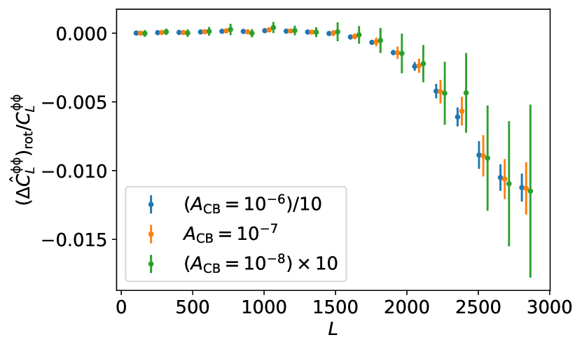
Figure 4: Comparing biases from different $A_{\rm CB}$ in a CMB-S4-like experiment. For visualization we have scaled both data and error bar by a factor of 10 and 0.1 for $A_{\rm CB}=10^{-8}$ and $10^{-6}$, respectively. Similarly the horizontal displacements between the three data series are for visualization purpose only.

Multiple methods for mitigating biases in CMB lensing measurements have been proposed. For example, the bias-hardening approach Namikawa et al. (2013); Namikawa and Takahashi (2014a); Osborne et al. (2014); Sailer et al. (2020) has been used to mitigate the mean-field bias in the reconstructed lensing map. In our case, however, this approach does not apply since the leading-order rotation fields do not produce mean-field bias in the reconstructed lensing map (see Eq. (38)). A simple approach to mitigating the rotation-induced bias arising from the connected four-point correlation is to first reconstruct the rotation fields using the quadratic estimator similar to the lensing reconstruction Gluscevic et al. (2009); Yadav et al. (2010) and then to de-rotate polarization maps using the reconstructed rotation fields, as originally proposed by Kamionkowski (2009). We leave a detailed analysis of the effectiveness of this approach to future work.

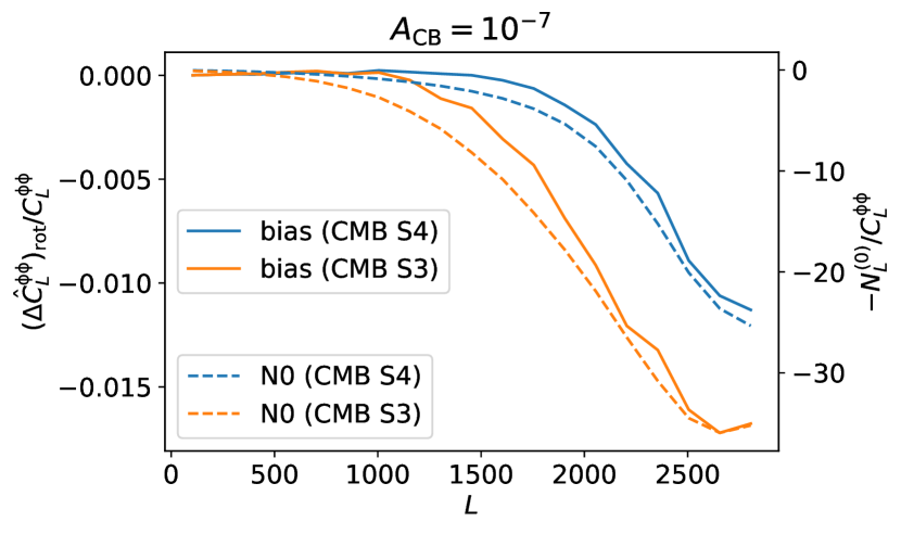
Figure 5: Comparing the observed bias (solid lines) with $-N^{(0)}_{L}/C_{L}^{\phi\phi}$ (dashed lines), where $N_{L}^{(0)}$ is obtained by averaging the ${}^{\rm(RD)}N^{(0)}$ from the lensed simulations (without rotation). Note that as mentioned in Sec. IV, ${}^{\rm(RD)}N^{(0)}$ only contains contribution from cosmic variance of CMB maps. The minus sign in front of $N_{L}^{(0)}$ is added to aid visual comparison.

VI Conclusion

The CMB lensing power spectrum encodes a wealth of information of matter fluctuations over a broad range of redshifts. Bias to the CMB lensing power spectrum may thus lead to bias in the cosmological parameters extracted from it. For example, the sum of neutrino masses can be constrained using CMB lensing power spectrum as massive neutrino can suppress CMB lensing power spectrum by several percent due to its suppression effect on the matter power spectrum below the neutrino free-streaming scale De Bernardis et al. (2009); Abazajian et al. (2015); it has also been shown in Ade et al. (2016) that bias in the high-$L$ ($L\gtrsim 1000$) may lead to bias in $\sigma_{8}\Omega_{\mathrm{m}}^{0.25}$ at $1\sigma$ level. Therefore, bias to the CMB lensing power spectrum needs to be carefully accounted for when constraining cosmological parameters.

In this paper we investigated the bias from anisotropic polarization rotation to the reconstructed CMB lensing power spectrum using the EB estimator. This bias has previously been investigated in the context of instrumental systematics Mirmelstein et al. (2021); Nagata and Namikawa (2021). In this work we focus instead on a particular class of physically motivated models that produce anisotropic cosmic birefringence, such as axion-like particles coupling to photons through Chern-Simons interaction or primordial magnetic field. In addition, we aim to identify the dominant terms responsible for the rotation-induced bias to CMB lensing.

Our results show that scale-invariant anisotropic cosmic birefringence with $A_{\rm CB}=10^{-7}$ can induce a percent-level bias to reconstructed CMB lensing power spectrum at small scales ($L>1000$) for both CMB-S3-like and CMB-S4-like experiments, and the bias scales linearly with $A_{\rm CB}$. This effect can be detectable (i.e. SNR$\geq 1$) if $A_{\rm CB}=5\times 10^{-7}$ with CMB-S4-like noise level.

We also found that the observed bias likely arises from the the connected terms in the CMB four-point correlation function induced by the leading-order perturbation from rotation; this explains the linear scaling of the bias with $A_{\rm CB}$. Polarization-based lensing reconstruction is expected to dominate or contribute substantially to the statistical power in CMB lensing reconstruction in the next generation CMB experiments. Rotation-induced bias to the CMB lensing power spectrum, therefore, may lead to non-negligible bias in the constraints of cosmological parameters such as the sum of neutrino masses and $\sigma_{8}$ and poses a significant challenge to achieving the science goals in future CMB lensing analysis. Thus, a possible rotation field is an important factor to account for and mitigate during lensing reconstruction. We argued that the bias-hardened estimator approach to mitigate bias does not work for rotation-induced bias, because of the orthogonality between rotation and CMB lensing. A promising mitigation method is to first reconstruct the anisotropic rotation field and then de-rotate the CMB polarization field with the reconstructed rotation field before proceeding to lensing reconstruction, but its effectiveness in the presence of galactic foreground and partial sky coverage remains to be seen.

As we have demonstrated in this paper, the reconstructed lensing power spectrum is highly sensitive to the level of anisotropic cosmic birefringence. Although this lensing bias is by itself not significant enough (SNR $\approx 0.2~{}\sigma$ for $A_{\mathrm{CB}}=10^{-7}$ with CMB-S4-like noise level) to be used as a probe for cosmic birefringence signal, jointly estimating cosmic birefringence and CMB lensing once maps get to low enough noise levels may still provide a useful consistency check should a cosmic birefringence signal be detected in the future.

Appendix A Realization-dependent Gaussian noise (RDN0)

Here we review the realization-dependent Gaussian noise (RDN0) applied in Eq. (43) and (44). RND0 is introduced in Namikawa et al. (2013); Namikawa and Takahashi (2014b) as a robust way to evaluate the reconstruction noise to CMB lensing power spectrum sourced by the disconnected terms of CMB four-point function (Gaussian noise). It has been applied in the CMB lensing power spectrum measurements of different experiments including Planck Collaboration et al. (2014); van Engelen et al. (2015); BICEP2 Collaboration et al. (2016)). In this section, we revisit the derivation of RDN0. We will adopt the flat-sky approximation in Namikawa et al. (2013), but the result applies to both flat-sky and full-sky analyses.

We start by defining the Gaussian probability distribution function (PDF) of the unlensed CMB multipoles as

$$P_{\mathrm{g}}=\frac{1}{\sqrt{(2\pi)^{N}\det C}}\exp\left(-\frac{1}{2}\sum_{ab}\sum_{\bm{\ell}\bm{\ell}^{\prime}}a_{\bm{\ell}}\left(\mathrm{C}^{-1}\right)^{a_{\bm{\ell}},b_{\bm{\ell}^{\prime}}}b_{\bm{\ell}^{\prime}}\right),$$ (52)

where $C$ is the covariance matrix between CMB multipoles, $a_{\bm{\ell}},b_{\bm{\ell}^{\prime}}$ represent the CMB multipoles, and $a,b\in\{T,E,B\}$.

When CMB fields are distorted by weak lensing, CMB multipoles become weakly non-Gaussian. The PDF of the lensed CMB multipoles can then be approximated using the Edgeworth expansion as Amendola (1996); Regan et al. (2010)

$$P \approx\left[1+\sum_{abcd}\sum_{\{\bm{\ell}_{i}\}}\left\langle a_{\bm{\ell}_{1}}b_{\bm{\ell}_{2}}c_{\bm{\ell}_{3}}d_{\bm{\ell}_{4}}\right\rangle_{c}\frac{\partial}{\partial a_{\bm{\ell}_{1}}}\frac{\partial}{\partial b_{\bm{\ell}_{2}}}\frac{\partial}{\partial c_{\bm{\ell}_{3}}}\frac{\partial}{\partial d_{\bm{\ell}_{4}}}\right]P_{\mathrm{g}},$$ (53)

where $\left\langle a_{\bm{\ell}_{1}}b_{\bm{\ell}_{2}}c_{\bm{\ell}_{3}}d_{\bm{\ell}_{4}}\right\rangle_{c}$ represents the connected terms (also known as cumulants or trispectrum) contributed by CMB lensing, given by Namikawa and Takahashi (2014b)

$$\left\langle a_{\bm{\ell}_{1}}b_{\bm{\ell}_{2}}c_{\bm{\ell}_{3}}d_{\bm{\ell}_{4}}\right\rangle_{\mathrm{c}}\approx ~{}f_{\bm{\ell}_{12},\bm{\ell}_{1}}^{ab}f_{-\bm{\ell}_{12},\bm{\ell}_{3}}^{cd}C_{\left|\bm{\ell}_{12}\right|}^{\phi\phi}\delta_{\bm{\ell}_{12},-\bm{\ell}_{34}}$$ (54)

$$+f_{\bm{\ell}_{13},\bm{\ell}_{1}}^{ac}f_{-\bm{\ell}_{13},\bm{\ell}_{2}}^{bd}C_{\left|\bm{\ell}_{13}\right|}^{\phi\phi}\delta_{\bm{\ell}_{13},-\bm{\ell}_{24}}$$

$$+f_{\bm{\ell}_{14},\bm{\ell}_{1}}^{ad}f_{-\bm{\ell}_{14},\bm{\ell}_{2}}^{bc}C_{\left|\bm{\ell}_{14}\right|}^{\phi\phi}\delta_{\bm{\ell}_{14},-\bm{\ell}_{23}},$$

to the leading order of $C_{L}^{\phi\phi}$, where $\bm{\ell}_{ij}\equiv\bm{\ell}_{i}+\bm{\ell}_{j}$, and $f_{\bm{\ell},\bm{\ell}^{\prime}}^{ab}$ represents the weight functions for lensing potential as in Namikawa and Takahashi (2014b).

We can then obtain an optimal estimator, $\widehat{C}_{L}^{\phi\phi}$, by maximizing the log-likelihood, ${\mathcal{L}}\equiv\ln P$, with

$$\frac{\partial\mathcal{L}}{\partial C^{\phi\phi}_{L}}\left(\widehat{C}_{L}^{\phi\phi}\right)=0,$$ (55)

and get Namikawa and Takahashi (2014b)

$$\widehat{C}_{L}^{\phi\phi}\propto\sum_{abcd}\sum_{|\bm{L}|=L}P_{g}^{-1}\left(\widehat{f}_{\bm{L}}^{ab}\widehat{f}_{-\bm{L}}^{cd}+\widehat{f}_{\bm{L}}^{ac}\widehat{f}_{-\bm{L}}^{bd}+\widehat{f}_{\bm{L}}^{ad}\widehat{f}_{-\bm{L}}^{bc}\right)P_{\mathrm{g}},$$ (56)

where we have defined

$$\widehat{f}_{\bm{L}}^{ab}\equiv\sum_{\bm{\ell}^{\prime}}f_{\bm{L},\bm{\ell}^{\prime}}^{ab}\frac{\partial}{\partial a_{\bm{L}}}\frac{\partial}{\partial b_{\bm{L}-\bm{\ell}^{\prime}}},$$ (57)

and have omitted the normalization. One can further show that

$$\widehat{f}_{\bm{L}}^{ab}P_{\mathrm{g}}=\left(\bar{x}_{\bm{L}}^{ab}-\left\langle\bar{x}_{\bm{L}}^{ab}\right\rangle\right)P_{\mathrm{g}},$$ (58)

where

$$\bar{x}_{\bm{L}}^{ab}\equiv\sum_{\bm{\ell}}f_{\bm{L},\bm{\ell}}^{ab}\bar{a}_{\bm{\ell}}\bar{b}_{\bm{L}-\bm{\ell}},$$ (59)

in which $\bar{a}_{\bm{\ell}}=\sum_{a^{\prime},\bm{\ell^{\prime}}}C^{-1}_{a_{\bm{\ell}}a^{\prime}_{\bm{\ell}^{\prime}}}a^{\prime}_{\bm{\ell}^{\prime}}$ represents the inverse-variance filtered CMB multipoles. Note that $\bar{x}_{\bm{L}}^{ab}$ resembles the unnormalized quadratic estimator for CMB lensing, and $\left\langle\bar{x}_{\bm{L}}^{ab}\right\rangle$ the mean-field bias.

One can further show that

$$P_{g}^{-1}\widehat{f}_{\bm{L}}^{ab}\widehat{f}_{-\bm{L}}^{cd}P_{\mathrm{g}}\propto\left[\left(\bar{x}_{\bm{L}}^{ab}-\left\langle\bar{x}_{\bm{L}}^{ab}\right\rangle\right)\left(\bar{x}_{{\color[rgb]{1,0,1}-}\bm{L}}^{cd}-\left\langle\bar{x}_{{\color[rgb]{1,0,1}-}\bm{L}}^{cd}\right\rangle\right)-n_{\bm{L}}^{ab,cd}\right],$$ (60)

with

$$n_{\bm{L}}^{ab,cd}\equiv \sum_{\bm{\ell}_{1},\bm{\ell}_{2}}f_{\bm{L},\bm{\ell}_{1}}^{ab}f_{\bm{-L},\bm{\ell}_{2}}^{cd}\times$$ (61)

$$( \bar{b}_{\bm{L}-\bm{\ell}_{1}}\bar{d}_{\bm{-L}-\bm{\ell}_{1}}C^{-1}_{a_{\bm{\ell}_{1}},c_{\bm{\ell}_{2}}}+\bar{b}_{\bm{L}-\bm{\ell}_{1}}\bar{c}_{\bm{-L}-\bm{\ell}_{1}}C^{-1}_{a_{\bm{\ell}_{1}},d_{\bm{\ell}_{2}}}$$

$$+ \bar{a}_{\bm{L}-\bm{\ell}_{1}}\bar{d}_{\bm{-L}-\bm{\ell}_{1}}C^{-1}_{b_{\bm{\ell}_{1}},c_{\bm{\ell}_{2}}}+\bar{a}_{\bm{L}-\bm{\ell}_{1}}\bar{c}_{\bm{-L}-\bm{\ell}_{1}}C^{-1}_{b_{\bm{\ell}_{1}},d_{\bm{\ell}_{2}}})$$

$$- \frac{1}{2}\sum_{\bm{\ell}_{1},\bm{\ell}_{2}}f_{\bm{L},\bm{\ell}_{1}}^{ab}f_{\bm{-L},\bm{\ell}_{2}}^{cd}\times$$

$$( C^{-1}_{a_{\bm{\ell}_{1}},c_{\bm{\ell}_{2}}}C^{-1}_{b_{\bm{L}-\bm{\ell}_{1}},d_{\bm{-L}-\bm{\ell}_{2}}}+C^{-1}_{a_{\bm{\ell}_{1}},d_{\bm{\ell}_{2}}}C^{-1}_{b_{\bm{L}-\bm{\ell}_{1}},c_{\bm{-L}-\bm{\ell}_{2}}}$$

$$+ C^{-1}_{b_{\bm{\ell}_{1}},c_{\bm{\ell}_{2}}}C^{-1}_{a_{\bm{L-\ell}_{1}},d_{\bm{-L-\ell}_{2}}}+C^{-1}_{b_{\bm{\ell}_{1}},d_{\bm{\ell}_{2}}}C^{-1}_{a_{\bm{L-\ell}_{1}},c_{\bm{-L-\ell}_{2}}}),$$

where we have used

$$C^{-1}_{a_{\bm{\ell}}a^{\prime}_{\bm{\ell}^{\prime}}}=\langle\bar{a}_{\bm{\ell}}\bar{a}^{\prime}_{\bm{\ell}^{\prime}}\rangle.$$ (62)

With Eq. (60), the optimal estimator for CMB lensing potential in Eq. (56) becomes

$$\widehat{C}_{L}^{\phi\phi}\propto \sum_{abcd}\sum_{|\bm{L}|=L}\bigg{(}\left[\left(\bar{x}_{\bm{L}}^{ab}-\left\langle\bar{x}_{\bm{L}}^{ab}\right\rangle\right)\left(\bar{x}_{{\color[rgb]{1,0,1}-}\bm{L}}^{cd}-\left\langle\bar{x}_{{\color[rgb]{1,0,1}-}\bm{L}}^{cd}\right\rangle\right)-n_{\bm{L}}^{ab,cd}\right]$$ (63)

$$+[b\leftrightarrow c]+[b\leftrightarrow d]\bigg{)}.$$

Note that $\bar{a},\bar{b},\bar{c},\bar{d}$ in Eq. (61) correspond to filtered CMB multipoles from data, whereas the covariance matrices, e.g., $C_{a_{\bm{\ell}_{1}},c_{\bm{\ell}_{2}}}$, are to be estimated from simulations. In particular, we apply two sets of Monte-Carlo CMB realizations based on the same fiducial cosmological model to estimate the covariance matrix, denoted as $S_{1}$ and $S_{2}$. Specifically, $S_{1}$ is used to estimate the covariance matrices in the first parentheses of Eq. (61); each product of covariance matrices in the second parenthesis of Eq. (61) is estimated using S1 and S2 respectively (i.e., $C^{-1}_{S1}C^{-1}_{S2}$). This way of estimating the covariance matrix is less sensitive to errors in the covariance matrix from statistical uncertainties as well as mis-modeling. To see that, we can express the estimated covariance matrix as $\hat{C}=\bar{C}+\Delta C$, with $\bar{C}$ the true covariance matrix and $\Delta C$ the error. It is then easy to check that, when averaging over different CMB realizations, the error in covariance matrix, $\Delta C$, does not contribute to $\langle n_{\bm{L}}^{ab,cd}\rangle$ in the leading order. Since $S_{1}$ and $S_{2}$ are assumed to be independent, statistical uncertainties in $\hat{C}$ will also be eliminated up to $O((\Delta C)^{2})$.

Incorporating the estimation of covariance matrices using $S_{1}$ and $S_{2}$, Eq. (61) can be expressed more succinctly as

$$n_{\bm{L}}^{ab,cd} =\left\langle\left(\bar{x}_{\bm{L}}^{a^{S_{1}}b}+\bar{x}_{\bm{L}}^{ab^{S_{1}}}\right)\left(\bar{x}_{-\bm{L}}^{c^{S_{1}}d}+\bar{x}_{-\bm{L}}^{cd^{S_{1}}}\right)\right\rangle_{S_{1}}-$$ (64)

$$\frac{1}{2}\left\langle\left(\bar{x}_{\bm{L}}^{a^{S_{1}}b^{S_{2}}}+\bar{x}_{\bm{L}}^{a^{S_{2}}b^{S_{1}}}\right)\left(\bar{x}_{-\bm{L}}^{c^{S_{1}}d^{S_{2}}}+\bar{x}_{-\bm{L}}^{c^{S_{2}}d^{S_{1}}}\right)\right\rangle_{S_{1},S_{2}},$$

where the superscripts $S_{i}$ denote the CMB simulation provided by the set of $S_{i}$, and $\langle...\rangle_{S_{i}}$ represents the average over the realizations of $S_{i}$. Adding back the omitted normalization in Eq. (64), and the omitted normalization, we obtain the realization-dependent Gaussian noise (RDN0) with a given set of $\{ab,cd\}$ as

$${}^{(\mathrm{RD})}\mathrm{N}^{(0)ab,cd}_{L}\propto \sum_{|\bm{L}|=L}n_{\bm{L}}^{ab,cd}$$ (65)

$$= ~{}\langle C_{L}^{\hat{\phi}\hat{\phi}}[ab^{S_{1}},cd^{S_{1}}]+C_{L}^{\hat{\phi}\hat{\phi}}[a^{S_{1}}b,ab^{S_{1}}]$$

$$+C_{L}^{\hat{\phi}\hat{\phi}}[a^{S_{1}}b,c^{S_{1}}d]+C_{L}^{\hat{\phi}\hat{\phi}}[ab^{S_{1}},c^{S_{1}}d]$$

$$-C_{L}^{\hat{\phi}\hat{\phi}}[a^{S_{1}}b^{S_{2}},c^{S_{1}}d^{S_{2}}]$$

$$-C_{L}^{\hat{\phi}\hat{\phi}}[a^{S_{1}}b^{S_{2}},c^{S_{2}}d^{S_{1}}]\rangle_{S_{1},S_{2}}.$$

In the context of this paper, we set $a=c=E$, $b=d=B$. $S_{1}$ and $S_{2}$ are two sets of independent lensed CMB realizations based on the fiducial cosmological model which does not include the cosmic birefringence effect. As a result, for the lensed-only data maps, the RDN0 is given by Eq. (43); for the rotated-lensed data maps, the RDN0 is given by Eq. (44).

Note that by averaging ${}^{\rm{(RD)}}\mathrm{N}^{(0)}_{L}$ over many CMB realisations, we reproduce the naive Gaussian reconstruction noise $\mathrm{N}^{(0)}_{L}$. However, one can see that ${}^{\rm{(RD)}}\mathrm{N}^{(0)}_{L}$ is more optimal because it preserves the critical realisation-dependent information which is lost in $\mathrm{N}^{(0)}_{L}$ after averaging. In addition, as previously discussed, RDN0 is also less sensitive to the errors in the covariance matrix such as the statistical uncertainties from the limited set of simulations used to calculate the covariance matrix and errors in the underlying fiducial model used to generate the simulations. It has been demonstrated in Madhavacheril et al. (2020) that such an error in covariance matrix may lead to a catastrophic error (see Fig. 2 of Madhavacheril et al. (2020)) in the estimated lensing power spectrum if the naive $N_{L}^{(0)}$ is used, and it is significantly reduced with RDN0.

References

- Hu and Okamoto (2002) W. Hu and T. Okamoto, ApJ 574, 566 (2002), arXiv:astro-ph/0111606 [astro-ph] .
- Okamoto and Hu (2003) T. Okamoto and W. Hu, Phys. Rev. D 67, 083002 (2003), arXiv:astro-ph/0301031 [astro-ph] .
- Planck Collaboration et al. (2020) Planck Collaboration, N. Aghanim, Y. Akrami, M. Ashdown, J. Aumont, C. Baccigalupi, M. Ballardini, A. J. Banday, R. B. Barreiro, N. Bartolo, S. Basak, K. Benabed, J. P. Bernard, M. Bersanelli, P. Bielewicz, J. J. Bock, J. R. Bond, J. Borrill, F. R. Bouchet, F. Boulanger, M. Bucher, C. Burigana, E. Calabrese, J. F. Cardoso, J. Carron, A. Challinor, H. C. Chiang, L. P. L. Colombo, C. Combet, B. P. Crill, F. Cuttaia, P. de Bernardis, G. de Zotti, J. Delabrouille, E. Di Valentino, J. M. Diego, O. Doré, M. Douspis, A. Ducout, X. Dupac, G. Efstathiou, F. Elsner, T. A. Enßlin, H. K. Eriksen, Y. Fantaye, R. Fernandez-Cobos, F. Finelli, F. Forastieri, M. Frailis, A. A. Fraisse, E. Franceschi, A. Frolov, S. Galeotta, S. Galli, K. Ganga, R. T. Génova-Santos, M. Gerbino, T. Ghosh, J. González-Nuevo, K. M. Górski, S. Gratton, A. Gruppuso, J. E. Gudmundsson, J. Hamann, W. Handley, F. K. Hansen, D. Herranz, E. Hivon, Z. Huang, A. H. Jaffe, W. C. Jones, A. Karakci, E. Keihänen, R. Keskitalo, K. Kiiveri, J. Kim, L. Knox, N. Krachmalnicoff, M. Kunz, H. Kurki-Suonio, G. Lagache, J. M. Lamarre, A. Lasenby, M. Lattanzi, C. R. Lawrence, M. Le Jeune, F. Levrier, A. Lewis, M. Liguori, P. B. Lilje, V. Lindholm, M. López-Caniego, P. M. Lubin, Y. Z. Ma, J. F. Macías-Pérez, G. Maggio, D. Maino, N. Mandolesi, A. Mangilli, A. Marcos-Caballero, M. Maris, P. G. Martin, E. Martínez-González, S. Matarrese, N. Mauri, J. D. McEwen, A. Melchiorri, A. Mennella, M. Migliaccio, M. A. Miville-Deschênes, D. Molinari, A. Moneti, L. Montier, G. Morgante, A. Moss, P. Natoli, L. Pagano, D. Paoletti, B. Partridge, G. Patanchon, F. Perrotta, V. Pettorino, F. Piacentini, L. Polastri, G. Polenta, J. L. Puget, J. P. Rachen, M. Reinecke, M. Remazeilles, A. Renzi, G. Rocha, C. Rosset, G. Roudier, J. A. Rubiño-Martín, B. Ruiz-Granados, L. Salvati, M. Sandri, M. Savelainen, D. Scott, C. Sirignano, R. Sunyaev, A. S. Suur-Uski, J. A. Tauber, D. Tavagnacco, M. Tenti, L. Toffolatti, M. Tomasi, T. Trombetti, J. Valiviita, B. Van Tent, P. Vielva, F. Villa, N. Vittorio, B. D. Wandelt, I. K. Wehus, M. White, S. D. M. White, A. Zacchei, and A. Zonca, A&A 641, A8 (2020), arXiv:1807.06210 [astro-ph.CO] .
- Planck Collaboration et al. (2014) Planck Collaboration, P. A. R. Ade, N. Aghanim, C. Armitage-Caplan, M. Arnaud, M. Ashdown, F. Atrio-Barandela, J. Aumont, C. Baccigalupi, A. J. Banday, and et al., A&A 571, A17 (2014), arXiv:1303.5077 [astro-ph.CO] .
- Carron et al. (2022) J. Carron, M. Mirmelstein, and A. Lewis, arXiv e-prints , arXiv:2206.07773 (2022), arXiv:2206.07773 [astro-ph.CO] .
- van Engelen et al. (2015) A. van Engelen, B. D. Sherwin, N. Sehgal, G. E. Addison, R. Allison, N. Battaglia, F. de Bernardis, J. R. Bond, E. Calabrese, K. Coughlin, D. Crichton, R. Datta, M. J. Devlin, J. Dunkley, R. Dünner, P. Gallardo, E. Grace, M. Gralla, A. Hajian, M. Hasselfield, S. Henderson, J. C. Hill, M. Hilton, A. D. Hincks, R. Hlozek, K. M. Huffenberger, J. P. Hughes, B. Koopman, A. Kosowsky, T. Louis, M. Lungu, M. Madhavacheril, L. Maurin, J. McMahon, K. Moodley, C. Munson, S. Naess, F. Nati, L. Newburgh, M. D. Niemack, M. R. Nolta, L. A. Page, C. Pappas, B. Partridge, B. L. Schmitt, J. L. Sievers, S. Simon, D. N. Spergel, S. T. Staggs, E. R. Switzer, J. T. Ward, and E. J. Wollack, ApJ 808, 7 (2015), arXiv:1412.0626 [astro-ph.CO] .
- BICEP2 Collaboration et al. (2016) BICEP2 Collaboration, Keck Array Collaboration, P. A. R. Ade, Z. Ahmed, R. W. Aikin, K. D. Alexander, D. Barkats, S. J. Benton, C. A. Bischoff, J. J. Bock, R. Bowens-Rubin, J. A. Brevik, I. Buder, E. Bullock, V. Buza, J. Connors, B. P. Crill, L. Duband, C. Dvorkin, J. P. Filippini, S. Fliescher, J. Grayson, M. Halpern, S. Harrison, S. R. Hildebrandt, G. C. Hilton, H. Hui, K. D. Irwin, J. Kang, K. S. Karkare, E. Karpel, J. P. Kaufman, B. G. Keating, S. Kefeli, S. A. Kernasovskiy, J. M. Kovac, C. L. Kuo, E. M. Leitch, M. Lueker, K. G. Megerian, T. Namikawa, C. B. Netterfield, H. T. Nguyen, R. O’Brient, I. Ogburn, R. W., A. Orlando, C. Pryke, S. Richter, R. Schwarz, C. D. Sheehy, Z. K. Staniszewski, B. Steinbach, R. V. Sudiwala, G. P. Teply, K. L. Thompson, J. E. Tolan, C. Tucker, A. D. Turner, A. G. Vieregg, A. C. Weber, D. V. Wiebe, J. Willmert, C. L. Wong, W. L. K. Wu, and K. W. Yoon, ApJ 833, 228 (2016), arXiv:1606.01968 [astro-ph.CO] .
- Polarbear Collaboration et al. (2014) Polarbear Collaboration, P. A. R. Ade, Y. Akiba, A. E. Anthony, K. Arnold, M. Atlas, D. Barron, D. Boettger, J. Borrill, S. Chapman, Y. Chinone, M. Dobbs, T. Elleflot, J. Errard, G. Fabbian, C. Feng, D. Flanigan, A. Gilbert, W. Grainger, N. W. Halverson, M. Hasegawa, K. Hattori, M. Hazumi, W. L. Holzapfel, Y. Hori, J. Howard, P. Hyland, Y. Inoue, G. C. Jaehnig, A. H. Jaffe, B. Keating, Z. Kermish, R. Keskitalo, T. Kisner, M. Le Jeune, A. T. Lee, E. M. Leitch, E. Linder, M. Lungu, F. Matsuda, T. Matsumura, X. Meng, N. J. Miller, H. Morii, S. Moyerman, M. J. Myers, M. Navaroli, H. Nishino, A. Orlando, H. Paar, J. Peloton, D. Poletti, E. Quealy, G. Rebeiz, C. L. Reichardt, P. L. Richards, C. Ross, I. Schanning, D. E. Schenck, B. D. Sherwin, A. Shimizu, C. Shimmin, M. Shimon, P. Siritanasak, G. Smecher, H. Spieler, N. Stebor, B. Steinbach, R. Stompor, A. Suzuki, S. Takakura, T. Tomaru, B. Wilson, A. Yadav, and O. Zahn, ApJ 794, 171 (2014), arXiv:1403.2369 [astro-ph.CO] .
- POLARBEAR Collaboration et al. (2017) POLARBEAR Collaboration, P. A. R. Ade, M. Aguilar, Y. Akiba, K. Arnold, C. Baccigalupi, D. Barron, D. Beck, F. Bianchini, D. Boettger, J. Borrill, S. Chapman, Y. Chinone, K. Crowley, A. Cukierman, R. Dünner, M. Dobbs, A. Ducout, T. Elleflot, J. Errard, G. Fabbian, S. M. Feeney, C. Feng, T. Fujino, N. Galitzki, A. Gilbert, N. Goeckner-Wald, J. C. Groh, G. Hall, N. Halverson, T. Hamada, M. Hasegawa, M. Hazumi, C. A. Hill, L. Howe, Y. Inoue, G. Jaehnig, A. H. Jaffe, O. Jeong, D. Kaneko, N. Katayama, B. Keating, R. Keskitalo, T. Kisner, N. Krachmalnicoff, A. Kusaka, M. Le Jeune, A. T. Lee, E. M. Leitch, D. Leon, E. Linder, L. Lowry, F. Matsuda, T. Matsumura, Y. Minami, J. Montgomery, M. Navaroli, H. Nishino, H. Paar, J. Peloton, A. T. P. Pham, D. Poletti, G. Puglisi, C. L. Reichardt, P. L. Richards, C. Ross, Y. Segawa, B. D. Sherwin, M. Silva-Feaver, P. Siritanasak, N. Stebor, R. Stompor, A. Suzuki, O. Tajima, S. Takakura, S. Takatori, D. Tanabe, G. P. Teply, T. Tomaru, C. Tucker, N. Whitehorn, and A. Zahn, ApJ 848, 121 (2017), arXiv:1705.02907 [astro-ph.CO] .
- van Engelen et al. (2012) A. van Engelen, R. Keisler, O. Zahn, K. A. Aird, B. A. Benson, L. E. Bleem, J. E. Carlstrom, C. L. Chang, H. M. Cho, T. M. Crawford, A. T. Crites, T. de Haan, M. A. Dobbs, J. Dudley, E. M. George, N. W. Halverson, G. P. Holder, W. L. Holzapfel, S. Hoover, Z. Hou, J. D. Hrubes, M. Joy, L. Knox, A. T. Lee, E. M. Leitch, M. Lueker, D. Luong-Van, J. J. McMahon, J. Mehl, S. S. Meyer, M. Millea, J. J. Mohr, T. E. Montroy, T. Natoli, S. Padin, T. Plagge, C. Pryke, C. L. Reichardt, J. E. Ruhl, J. T. Sayre, K. K. Schaffer, L. Shaw, E. Shirokoff, H. G. Spieler, Z. Staniszewski, A. A. Stark, K. Story, K. Vanderlinde, J. D. Vieira, and R. Williamson, ApJ 756, 142 (2012), arXiv:1202.0546 [astro-ph.CO] .
- Story et al. (2015) K. T. Story, D. Hanson, P. A. R. Ade, K. A. Aird, J. E. Austermann, J. A. Beall, A. N. Bender, B. A. Benson, L. E. Bleem, J. E. Carlstrom, C. L. Chang, H. C. Chiang, H. M. Cho, R. Citron, T. M. Crawford, A. T. Crites, T. de Haan, M. A. Dobbs, W. Everett, J. Gallicchio, J. Gao, E. M. George, A. Gilbert, N. W. Halverson, N. Harrington, J. W. Henning, G. C. Hilton, G. P. Holder, W. L. Holzapfel, S. Hoover, Z. Hou, J. D. Hrubes, N. Huang, J. Hubmayr, K. D. Irwin, R. Keisler, L. Knox, A. T. Lee, E. M. Leitch, D. Li, C. Liang, D. Luong-Van, J. J. McMahon, J. Mehl, S. S. Meyer, L. Mocanu, T. E. Montroy, T. Natoli, J. P. Nibarger, V. Novosad, S. Padin, C. Pryke, C. L. Reichardt, J. E. Ruhl, B. R. Saliwanchik, J. T. Sayre, K. K. Schaffer, G. Smecher, A. A. Stark, C. Tucker, K. Vanderlinde, J. D. Vieira, G. Wang, N. Whitehorn, V. Yefremenko, and O. Zahn, ApJ 810, 50 (2015), arXiv:1412.4760 [astro-ph.CO] .
- Ade et al. (2019) P. Ade, J. Aguirre, Z. Ahmed, S. Aiola, A. Ali, et al., Journal of Cosmology and Astroparticle Physics 2019 (2019), 10.1088/1475-7516/2019/02/056, arXiv:1808.07445 .
- Abazajian et al. (2016) K. N. Abazajian, P. Adshead, Z. Ahmed, S. W. Allen, D. Alonso, et al., (2016), arXiv:1610.02743 .
- Abazajian et al. (2016) K. N. Abazajian, P. Adshead, Z. Ahmed, S. W. Allen, D. Alonso, K. S. Arnold, C. Baccigalupi, J. G. Bartlett, N. Battaglia, B. A. Benson, C. A. Bischoff, J. Borrill, V. Buza, E. Calabrese, R. Caldwell, J. E. Carlstrom, C. L. Chang, T. M. Crawford, F.-Y. Cyr-Racine, F. De Bernardis, T. de Haan, S. di Serego Alighieri, J. Dunkley, C. Dvorkin, J. Errard, G. Fabbian, S. Feeney, S. Ferraro, J. P. Filippini, R. Flauger, G. M. Fuller, V. Gluscevic, D. Green, D. Grin, E. Grohs, J. W. Henning, J. C. Hill, R. Hlozek, G. Holder, W. Holzapfel, W. Hu, K. M. Huffenberger, R. Keskitalo, L. Knox, A. Kosowsky, J. Kovac, E. D. Kovetz, C.-L. Kuo, A. Kusaka, M. Le Jeune, A. T. Lee, M. Lilley, M. Loverde, M. S. Madhavacheril, A. Mantz, D. J. E. Marsh, J. McMahon, P. D. Meerburg, J. Meyers, A. D. Miller, J. B. Munoz, H. N. Nguyen, M. D. Niemack, M. Peloso, J. Peloton, L. Pogosian, C. Pryke, M. Raveri, C. L. Reichardt, G. Rocha, A. Rotti, E. Schaan, M. M. Schmittfull, D. Scott, N. Sehgal, S. Shandera, B. D. Sherwin, T. L. Smith, L. Sorbo, G. D. Starkman, K. T. Story, A. van Engelen, J. D. Vieira, S. Watson, N. Whitehorn, and W. L. Kimmy Wu, arXiv e-prints , arXiv:1610.02743 (2016), arXiv:1610.02743 [astro-ph.CO] .
- Ferraro and Hill (2018) S. Ferraro and J. C. Hill, Physical Review D 97, 023512 (2018).
- Cai et al. (2022) H. Cai, M. S. Madhavacheril, J. C. Hill, and A. Kosowsky, Phys. Rev. D 105, 043516 (2022), arXiv:2111.01944 [astro-ph.CO] .
- Mirmelstein et al. (2021) M. Mirmelstein, G. Fabbian, A. Lewis, and J. Peloton, Phys. Rev. D 103, 123540 (2021), arXiv:2011.13910 [astro-ph.CO] .
- Nagata and Namikawa (2021) R. Nagata and T. Namikawa, Progress of Theoretical and Experimental Physics 2021, 053E01 (2021), arXiv:2102.00133 [astro-ph.CO] .
- Minami and Komatsu (2020) Y. Minami and E. Komatsu, Phys. Rev. Lett. 125, 221301 (2020), arXiv:2011.11254 [astro-ph.CO] .
- Diego-Palazuelos et al. (2022) P. Diego-Palazuelos et al., Phys. Rev. Lett. 128, 091302 (2022), arXiv:2201.07682 [astro-ph.CO] .
- Eskilt and Komatsu (2022) J. R. Eskilt and E. Komatsu, (2022), arXiv:2205.13962 [astro-ph.CO] .
- Komatsu (2022) E. Komatsu, Nature Rev. Phys. 4, 452 (2022), arXiv:2202.13919 [astro-ph.CO] .
- Sherwin and Namikawa (2021) B. D. Sherwin and T. Namikawa, arXiv e-prints , arXiv:2108.09287 (2021), arXiv:2108.09287 [astro-ph.CO] .
- Nakatsuka et al. (2022) H. Nakatsuka, T. Namikawa, and E. Komatsu, Phys. Rev. D 105, 123509 (2022), arXiv:2203.08560 [astro-ph.CO] .
- Lee et al. (2022) N. Lee, S. C. Hotinli, and M. Kamionkowski, (2022), arXiv:2207.05687 [astro-ph.CO] .
- Gasparotto and Obata (2022) S. Gasparotto and I. Obata, JCAP 08, 025 (2022), arXiv:2203.09409 [astro-ph.CO] .
- Capparelli et al. (2020) L. M. Capparelli, R. R. Caldwell, and A. Melchiorri, Phys. Rev. D 101, 123529 (2020), arXiv:1909.04621 [astro-ph.CO] .
- Fujita et al. (2020) T. Fujita, Y. Minami, K. Murai, and H. Nakatsuka, arXiv e-prints , arXiv:2008.02473 (2020), arXiv:2008.02473 [astro-ph.CO] .
- Kitajima et al. (2022) N. Kitajima, F. Kozai, F. Takahashi, and W. Yin, (2022), arXiv:2205.05083 [astro-ph.CO] .
- Jain et al. (2022) M. Jain, R. Hagimoto, A. J. Long, and M. A. Amin, (2022), arXiv:2208.08391 [astro-ph.CO] .
- Kamionkowski (2009) M. Kamionkowski, Phys. Rev. Lett. 102, 111302 (2009), arXiv:0810.1286 [astro-ph] .
- Goldberg et al. (1967) J. N. Goldberg, A. J. Macfarlane, E. T. Newman, F. Rohrlich, and E. C. Sudarshan, Journal of Mathematical Physics 8, 2155 (1967).
- Kamionkowski et al. (1997) M. Kamionkowski, A. Kosowsky, and A. Stebbins, Phys. Rev. Lett. 78, 2058 (1997), arXiv:astro-ph/9609132 .
- Zaldarriaga and Seljak (1997) M. Zaldarriaga and U. Seljak, Phys. Rev. D 55, 1830 (1997), arXiv:astro-ph/9609170 [astro-ph] .
- Lewis and Challinor (2006) A. Lewis and A. Challinor, Phys. Rept. 429, 1 (2006), arXiv:astro-ph/0601594 .
- Sherwin et al. (2017) B. D. Sherwin, A. van Engelen, N. Sehgal, M. Madhavacheril, G. E. Addison, S. Aiola, R. Allison, N. Battaglia, D. T. Becker, J. A. Beall, J. R. Bond, E. Calabrese, R. Datta, M. J. Devlin, R. Dünner, J. Dunkley, A. E. Fox, P. Gallardo, M. Halpern, M. Hasselfield, S. Henderson, J. C. Hill, G. C. Hilton, J. Hubmayr, J. P. Hughes, A. D. Hincks, R. Hlozek, K. M. Huffenberger, B. Koopman, A. Kosowsky, T. Louis, L. Maurin, J. McMahon, K. Moodley, S. Naess, F. Nati, L. Newburgh, M. D. Niemack, L. A. Page, J. Sievers, D. N. Spergel, S. T. Staggs, R. J. Thornton, J. Van Lanen, E. Vavagiakis, and E. J. Wollack, Phys. Rev. D 95, 123529 (2017), arXiv:1611.09753 [astro-ph.CO] .
- Carroll (1998) S. M. Carroll, Phys. Rev. Lett. 81, 3067 (1998), arXiv:astro-ph/9806099 [astro-ph] .
- Li and Zhang (2008) M. Li and X. Zhang, Phys. Rev. D 78, 103516 (2008), arXiv:0810.0403 [astro-ph] .
- Marsh (2016) D. J. E. Marsh, Phys. Rept. 643, 1 (2016), arXiv:1510.07633 [astro-ph.CO] .
- Leon et al. (2016) D. Leon, J. Kaufman, B. Keating, and M. Mewes, Mod. Phys. Lett. A 32, 1730002 (2016), arXiv:1611.00418 [astro-ph.CO] .
- Kosowsky and Loeb (1996) A. Kosowsky and A. Loeb, Astrophys. J. 469, 1 (1996), arXiv:astro-ph/9601055 .
- Harari et al. (1997) D. D. Harari, J. D. Hayward, and M. Zaldarriaga, Phys. Rev. D 55, 1841 (1997), arXiv:astro-ph/9608098 .
- Kosowsky et al. (2005) A. Kosowsky, T. Kahniashvili, G. Lavrelashvili, and B. Ratra, Phys. Rev. D 71, 043006 (2005), arXiv:astro-ph/0409767 .
- Yadav et al. (2012) A. Yadav, L. Pogosian, and T. Vachaspati, Phys. Rev. D 86, 123009 (2012), arXiv:1207.3356 [astro-ph.CO] .
- De et al. (2013) S. De, L. Pogosian, and T. Vachaspati, Phys. Rev. D 88, 063527 (2013), arXiv:1305.7225 [astro-ph.CO] .
- Pogosian (2014) L. Pogosian, Mon. Not. Roy. Astron. Soc. 438, 2508 (2014), arXiv:1311.2926 [astro-ph.CO] .
- Colladay and Kostelecký (1997) D. Colladay and V. A. Kostelecký, Phys. Rev. D 55, 6760 (1997), arXiv:hep-ph/9703464 [hep-ph] .
- Colladay and Kostelecký (1998) D. Colladay and V. A. Kostelecký, Phys. Rev. D 58, 116002 (1998), arXiv:hep-ph/9809521 [astro-ph] .
- Leon et al. (2017) D. Leon, J. Kaufman, B. Keating, and M. Mewes, Modern Physics Letters A 32, 1730002 (2017), arXiv:1611.00418 [astro-ph.CO] .
- Caldwell et al. (2011) R. R. Caldwell, V. Gluscevic, and M. Kamionkowski, Phys. Rev. D 84, 043504 (2011), arXiv:1104.1634 [astro-ph.CO] .
- Gluscevic et al. (2009) V. Gluscevic, M. Kamionkowski, and A. Cooray, Phys. Rev. D 80, 023510 (2009), arXiv:0905.1687 [astro-ph.CO] .
- Namikawa et al. (2020) T. Namikawa, Y. Guan, O. Darwish, B. D. Sherwin, S. Aiola, N. Battaglia, J. A. Beall, D. T. Becker, J. R. Bond, E. Calabrese, G. E. Chesmore, S. K. Choi, M. J. Devlin, J. Dunkley, R. Dünner, A. E. Fox, P. A. Gallardo, V. Gluscevic, D. Han, M. Hasselfield, G. C. Hilton, A. D. Hincks, R. Hložek, J. Hubmayr, K. Huffenberger, J. P. Hughes, B. J. Koopman, A. Kosowsky, T. Louis, M. Lungu, A. MacInnis, M. S. Madhavacheril, M. Mallaby-Kay, L. Maurin, J. McMahon, K. Moodley, S. Naess, F. Nati, L. B. Newburgh, J. P. Nibarger, M. D. Niemack, L. A. Page, F. J. Qu, N. Robertson, A. Schillaci, N. Sehgal, C. Sifón, S. M. Simon, D. N. Spergel, S. T. Staggs, E. R. Storer, A. van Engelen, J. van Lanen, and E. J. Wollack, Phys. Rev. D 101, 083527 (2020), arXiv:2001.10465 [astro-ph.CO] .
- Bianchini et al. (2020) F. Bianchini et al. (SPT), Phys. Rev. D 102, 083504 (2020), arXiv:2006.08061 [astro-ph.CO] .
- Aiola et al. (2022) S. Aiola et al. (CMB-HD), (2022), arXiv:2203.05728 [astro-ph.CO] .
- Pogosian et al. (2019) L. Pogosian, M. Shimon, M. Mewes, and B. Keating, Phys. Rev. D 100, 023507 (2019), arXiv:1904.07855 [astro-ph.CO] .
- Mandal et al. (2022) S. Mandal, N. Sehgal, and T. Namikawa, Phys. Rev. D 105, 063537 (2022), arXiv:2201.02204 [astro-ph.CO] .
- Gluscevic et al. (2009) V. Gluscevic, M. Kamionkowski, and A. Cooray, Physical Review D 80 (2009), 10.1103/physrevd.80.023510.
- Li and Yu (2013) M. Li and B. Yu, JCAP 06, 016 (2013), arXiv:1303.1881 [astro-ph.CO] .
- Cai and Guan (2022) H. Cai and Y. Guan, Phys. Rev. D 105, 063536 (2022), arXiv:2111.14199 [astro-ph.CO] .
- Namikawa et al. (2013) T. Namikawa, D. Hanson, and R. Takahashi, Monthly Notices of the Royal Astronomical Society 431, 609–620 (2013).
- Madhavacheril et al. (2020) M. S. Madhavacheril, K. M. Smith, B. D. Sherwin, and S. Naess, (2020), arXiv:2011.02475 [astro-ph.CO] .
- Naess et al. (2021) S. Naess, M. Madhavacheril, and M. Hasselfield, “Pixell: Rectangular pixel map manipulation and harmonic analysis library,” (2021), ascl:2102.003 .
- Planck Collaboration et al. (2018) Planck Collaboration, N. Aghanim, Y. Akrami, M. Ashdown, J. Aumont, et al., (2018), arXiv:1807.06209 .
- Pogosian et al. (2019) L. Pogosian, M. Shimon, M. Mewes, and B. Keating, Phys. Rev. D 100, 023507 (2019), arXiv:1904.07855 [astro-ph.CO] .
- Namikawa (2021) T. Namikawa, “cmblensplus: Cosmic microwave background tools,” Astrophysics Source Code Library, record ascl:2104.021 (2021), ascl:2104.021 .
- Knox (1995) L. Knox, Phys. Rev. D 52, 4307 (1995).
- Kesden et al. (2003) M. Kesden, A. Cooray, and M. Kamionkowski, Phys. Rev. D 67, 123507 (2003), arXiv:astro-ph/0302536 [astro-ph] .
- Hanson et al. (2011) D. Hanson, A. Challinor, G. Efstathiou, and P. Bielewicz, Phys. Rev. D 83, 043005 (2011).
- Namikawa and Takahashi (2014a) T. Namikawa and R. Takahashi, Mon. Not. Roy. Astron. Soc. 438, 1507 (2014a), arXiv:1310.2372 [astro-ph.CO] .
- Osborne et al. (2014) S. J. Osborne, D. Hanson, and O. Doré, JCAP 03, 024 (2014), arXiv:1310.7547 [astro-ph.CO] .
- Sailer et al. (2020) N. Sailer, E. Schaan, and S. Ferraro, Phys. Rev. D 102, 063517 (2020), arXiv:2007.04325 [astro-ph.CO] .
- Yadav et al. (2010) A. P. S. Yadav, M. Su, and M. Zaldarriaga, Phys. Rev. D 81, 063512 (2010), arXiv:0912.3532 [astro-ph.CO] .
- De Bernardis et al. (2009) F. De Bernardis, T. D. Kitching, A. Heavens, and A. Melchiorri, Phys. Rev. D 80, 123509 (2009), arXiv:0907.1917 [astro-ph.CO] .
- Abazajian et al. (2015) K. N. Abazajian et al. (Topical Conveners: K.N. Abazajian, J.E. Carlstrom, A.T. Lee), Astropart. Phys. 63, 66 (2015), arXiv:1309.5383 [astro-ph.CO] .
- Ade et al. (2016) P. A. R. Ade et al. (Planck), Astron. Astrophys. 594, A15 (2016), arXiv:1502.01591 [astro-ph.CO] .
- Zonca et al. (2019) A. Zonca, L. Singer, D. Lenz, M. Reinecke, C. Rosset, E. Hivon, and K. Gorski, The Journal of Open Source Software 4, 1298 (2019).
- Namikawa and Takahashi (2014b) T. Namikawa and R. Takahashi, Mon. Not. Roy. Astron. Soc. 438, 1507 (2014b), arXiv:1310.2372 [astro-ph.CO] .
- Amendola (1996) L. Amendola, Monthly Notices of the Royal Astronomical Society 283, 983 (1996), https://academic.oup.com/mnras/article-pdf/283/3/983/3305407/283-3-983.pdf .
- Regan et al. (2010) D. M. Regan, E. P. S. Shellard, and J. R. Fergusson, Phys. Rev. D 82, 023520 (2010).