Control Barrier Functions for Stochastic Systems With Quantitative Evaluation of Probability

Abstract

In recent years, the analysis of a control barrier function has received considerable attention because it is helpful for the safety-critical control required in many control application problems. However, the extension of the analysis to a stochastic system remains a challenging issue. In this paper, we consider sufficient conditions for reciprocal and zeroing control barrier functions ensuring safety with probability one and design a control law using the functions. Then, we propose another version of a stochastic zeroing control barrier function to evaluate a probability of a sample path staying in a safe set and confirm the convergence of a specific expectation related to the attractiveness of a safe set. We also discuss the robustness of safety against changing a diffusion coefficient. Finally, we confirm the validity of the proposed control design and the analysis using the control barrier functions via simple examples with their numerical simulation.

1 Introduction

In recent control application problems, opportunities for demands for sophisticated machine behavior and machine-to-human contact have increased. Because the problems require machine behavior to stay within a safe range for the machine itself and humans, the center of the control design guidelines is changing from stability to safety. The transition is theoretically realized by the change from stabilization based on a control Lyapunov function to safety-critical control based on a control barrier function (CBF) [1, 2]. In the last few years, research results on a CBF have been actively reported with various control application problems, and in reality, the simple realization of seemingly complicated commands [2, 3], and human assist control [4, 5, 6] are being promoted.

In the context of a CBF, the control objective is to make a specific subset, which is said to be a safe set, on the state space invariance forward in time (namely, forward invariance [2]). There are various types of CBFs, the most commonly used currently are a reciprocal control barrier function (RCBF) [2, 4, 5] and a zeroing control barrier function (ZCBF) [2, 3, 6]: the RCBF is a positive function that diverges from the inside of the safe set toward the boundary, while the ZCBF is a function that is zero at the boundary of the safe set. The RCBF has a form that is easy to imagine as a barrier, while the ZCBF is defined outside the safe set, allowing the design of control laws with robustness.

On the other hand, the aforementioned literature [1, 2, 3, 4, 5, 6] focuses on systems without stochastic disturbances. Because a stochastic disturbance often affects a real system, a safe set is desirable to maintain invariance even when influenced by the disturbance. Recently, various types of CBF-based stochastic safety-critical control have been proposed in [9, 10, 11, 7, 8, 12, 13]. For discrete-time stochastic systems, Jagtap et al. [7] conducts a systematic and detailed study, and then it is developed into a data-driven framework by Salamati and Zamani [8]. For continuous-time stochastic systems, Prajna et al. [9] provides a safety verification procedure, and then it is developed to control design procedure by Santoyo et al. [10]. Wisniewski and Bujorianu [11] also discuss in detail safety in an infinite time-horizon named $p$-stability.

The deterministic version of CBFs proposed by Ames et al. [2] is also extended to a stochastic version by Clark [12]; he also insists that his RCBF and ZCBF guarantee the safety of a set with probability one. At the same time, Wang et al. [13] analyze the probability of a time when the sample path leaves a safe set under conditions similar to Clark’s ZCBF. Wang et al. also claim that a state-feedback law achieving safety with probability one often diverges toward the boundary of the safe set; the inference is also obtained from the fact that the conditions for the existence of an invariance set in a stochastic system are strict and influenced by the properties of the diffusion coefficients [14]. Therefore, we need to reconsider a sufficient condition of safety with probability one, and we also need to rethink the problem setup to compute the safety probability obtained by a bounded control law.

In this paper, we propose a way of analyzing safety probability for a stochastic system via a CBF approach. The contributions of this paper are as follows. First, we propose an almost sure reciprocal control barrier function (AS-RCBF) ensuring the safety of a set with probability one, which is considered as a stochastic version of an extended RCBF in [5]; see also [4] ( and note that the condition is somewhat relaxed compared with an RCBF in [1]). Second, we propose an almost sure zeroing control barrier function (AS-ZCBF) satisfying an inequality somewhat different from the one in [12]. Then, we suggest a new stochastic ZCBF for explicitly calculating the safety probability of a set. Our stochastic ZCBF satisfies an inequality, which differs from the previous results in [9, 10, 11] because the inequality directly includes the diffusion coefficients. We also claim that the feature of the inequality is effective for calculating the safety probability under the diffusion coefficient change. In addition, we demonstrate our stochastic ZCBF is available for stochastic systems including input constraints by simple examples.

The rest of this paper is organized as follows. In Section 2, we define mathematical notations, a target system, and a global solution used in this paper. In Section 3, by considering a simple example, we confirm that a stochastic system is generally difficult to have a safe set invariance with probability one. In Section 4, first, we propose an AS-RCBF and an AS-ZCBF ensuring the invariance of a safe set with probability one. Second, we design a safety-critical control ensuring the existence of an AS-RCBF and an AS-ZCBF and show that the controller diverges towards the boundary of a safe set. Third, we construct a new type of a stochastic ZCBF clarifying a probability for the invariance of a safe set and showing the convergence of a specific expectation related to the attractiveness of a safe set from the outside of the set. And then, we discuss the conditions of an AS-ZCBF and a stochastic ZCBF, ensuring the safety against the change of a diffusion coefficient. In Section 5, we confirm the usefulness of the proposed functions and the control design via simple examples with numerical simulation. Section 6 concludes this paper.

2 Preliminary

2.1 Notations

Let ${\mathbb{R}}^{n}$ be an $n$-dimensional Euclidean space and especially ${\mathbb{R}}:={\mathbb{R}}^{1}$. A Lie derivative of a smooth mapping ${y}:{\mathbb{R}}^{n}\to{\mathbb{R}}$ in a mapping $F=(F_{1},\ldots,F_{q}):{\mathbb{R}}^{n}\to{\mathbb{R}}^{n\times q}$ with $F_{1},\ldots,F_{q}:{\mathbb{R}}^{n}\to{\mathbb{R}}^{n}$ is denoted by

$${\mathrm{L}_{F}{{y}}}(x)=\left({\dfrac{\partial{{y}}}{\partial{x}}}F_{1}(x),\ldots,{\dfrac{\partial{{y}}}{\partial{x}}}F_{q}(x)\right).$$ (1)

For constants $a,b>0$, a continuous mapping $\alpha:[-b,a]\to{\mathbb{R}}$ is said to be an extended class $\mathcal{K}$ function if it is strictly increasing and satisfies $\alpha(0)=0$. A class $\mathcal{K}$ function $\alpha$ is said to be of $\mathcal{K}_{\infty}$ if $\lim_{s\to\infty}\alpha(s)=\infty$. If a function $\alpha:{\mathbb{R}}^{n}\to{\mathbb{R}}$ is continuously differentiable for $r$-times, we state it as “$\alpha$ is $C^{r}$.” The boundary of a set $\mathcal{A}$ is denoted by $\partial\mathcal{A}$.

Let $(\Omega,\mathcal{F},\{\mathcal{F}_{t}\}_{t\geq 0},\mathbb{P})$ be a filtered probability space, where $\Omega$ is the sample space, $\mathcal{F}$ is the $\sigma$-algebra that is a collection of all the events, $\{\mathcal{F}_{t}\}_{t\geq 0}$ is a filtration of $\mathcal{F}$ and $\mathbb{P}$ is a probabilistic measure. In the filtered probability space, ${\mathbb{P}\left[{A|A_{o}}\right]}$ is the conditional probability of event $A$ conditioned on event $A_{o}$, ${\mathbb{E}\left[{y|A_{o}}\right]}$ is the conditional expectation of the random variable $y$ conditioned on event $A_{o}$, and $W_{t}$ is a $d$-dimensional standard Wiener process. For a Markov process ${X_{t}}\in{\mathbb{R}}^{n}$ with an initial state ${X_{t}}=x_{0}$, we often use the following notations ${\mathbb{P}_{x_{0}}\left[{A}\right]}={\mathbb{P}\left[{A|{X_{0}}=x_{0}}\right]}$ and ${\mathbb{E}_{x_{0}}\left[{y}\right]}={\mathbb{E}\left[{y|{X_{0}}=x_{0}}\right]}$. The minimum of $a,b\in{\mathbb{R}}$ is described by $a\wedge b:=\min(a,b)$. The differential form of an Itô integral of $f:{\mathbb{R}}^{n}\to{\mathbb{R}}^{n}$ over $W_{t}$ is represented by $f(x)d{W_{t}}$. The trace of a square matrix $Q$ is denoted by $\mathrm{tr}[{{Q}}]$.

2.2 Target system, the related functions, and a global solution

In this subsection, we describe a target system, the related functions frequently used throughout the paper, and the definition of a solution in global time.

The main target of this paper is the following stochastic system

$$d{X_{t}} =\{f({X_{t}})+g({X_{t}})(u_{o}({X_{t}})+u{(t)})\}dt+\sigma({X_{t}})d{W_{t}},$$ (2)

where $X_{t}\in{\mathbb{R}}^{n}$ is a state vector, $u_{o}:{\mathbb{R}}^{n}\to{\mathbb{R}}^{m}$ is a pre-input assumed to be a continuous state-feedback, $u\in U\subset{\mathbb{R}}^{m}$ is a compensator for safety-critical control, where $U$ denotes an acceptable control set, and maps $f:{\mathbb{R}}^{n}\to{\mathbb{R}}^{n}$ and $g:{\mathbb{R}}^{n}\to{\mathbb{R}}^{n}\times{\mathbb{R}}^{m}$ and $\sigma:{\mathbb{R}}^{n}\to{\mathbb{R}}^{n}\times{\mathbb{R}}^{d}$ are all assumed to be locally Lipschitz. The local Lipschitz condition of $f$, $g$ and $\sigma$ implies that there exists a stopping time $T>0$ such that $(X_{t})_{t<T}$ is the maximal solution to the system.

For simplicity, we further define some functions. For a $C^{2}$ mapping $y:M\to{\mathbb{R}}$, where $x\in$ $M\subset{\mathbb{R}}^{n}$, letting

$$L^{D}_{f,g}(u,u_{o}(x),y(x)):=({\mathrm{L}_{f}{y}})(x)+({\mathrm{L}_{g}{y}})(x)(u+u_{o}(x)),$$ (3)

$$L^{I}_{\sigma}(y(x)):=\frac{1}{2}\mathrm{tr}\left[\sigma(x)\sigma(x)^{T}\left[{\dfrac{\partial{}}{\partial{x}}}\left[{\dfrac{\partial{y}}{\partial{x}}}\right]^{T}\right](x)\right],$$ (4)

we consider an infinitesimal operator $\mathcal{L}$ in [16] satisfying

$$\mathcal{L}_{f,g,\sigma}(u,u_{o}(x),y(x)):=L^{D}_{f,g}(u,u_{o}(x),y(x))+L^{I}_{\sigma}(y(x))$$ (5)

and

$$H_{\sigma}(h(x)):=\frac{1}{2}{\mathrm{L}_{\sigma}{h}}(x)({\mathrm{L}_{\sigma}{h}}(x))^{T}.$$ (6)

For a mapping $v:M\to(0,\infty)$ smooth in $M\subset{\mathbb{R}}^{n}$, we often consider the relationship

$$-(v(x))^{-2}L^{D}_{f,g}(u,u_{o}(x),v(x))=L^{D}_{f,g}(u,u_{o}(x),(v(x))^{-1}).$$ (7)

Moreover, based on [15], we describe the following notion meaning the existence of a global solution in forward time for the system (2):

Definition 1 (FIiP and FCiP; a slight modification of (C2) in [15])

Let an open subset $M\subset{\mathbb{R}}^{n}$ and the system (2) be considered with $u=\phi(x)$, where $\phi:M\to{\mathbb{R}}^{n}$ is a continuous mapping. If a $C^{2}$ mapping $Y:M\to[0,\infty)$ is proper; that is, for any $L\in[0,\infty)$, any sublevel set $\{x\in M|Y(x)\leq L\}$ is compact, and a continuous mapping $\psi:[0,\infty)\times(0,1)\to[0,\infty)$ both exist for every $x_{0}\in M$ such that

$${\mathbb{P}_{x_{0}}\left[{\forall t\in[0,l],\ Y({X_{t}})\leq\psi(l,\epsilon)}\right]}\geq 1-\epsilon$$ (8)

holds for all $l\in[0,\infty)$ and all $\epsilon\in(0,1{]}$, then the system is said to be forward invariance in probability (FIiP) in $M$. In addition, if $M={\mathbb{R}}^{n}$ and $Y(\cdot)=|\cdot|$, the system is said to be forward complete in probability (FCiP). $\square$

Theorem 1

(A slight modification of Proposition 17 in [15]): Let us consider the system (2), an open subset $M\subset{\mathbb{R}}^{n}$, a continuous mapping $\phi:M\to{\mathbb{R}}^{n}$ and an initial condition $x_{0}\in M$. If there exists a proper and $C^{2}$ mapping $Y:M\to[0,\infty)$ such that

$$\mathcal{L}_{f,g,\sigma}(\phi(x),u_{o}(x),Y(x))\leq c_{1}Y(x)+c_{2}$$ (9)

is satisfied for all $x\in M$ and for some $c_{1}\in[0,\infty)$ and $c_{2}\in[0,\infty)$, then the system with $u=\phi(x)$ is FIiP in $M$. In addition, if $M={\mathbb{R}}^{n}$, the system is FCiP. $\blacklozenge$

Definition 1 and Theorem 1 are the same as (C2) and Proposition 17 in [15], respectively, except for two differences; $x$ is restricted in $M$ and $Y$ is allowed to be not positive definite in this paper, while $x$ is allowed to be in ${\mathbb{R}}^{n}$ and $Y$ is restricted to be positive definite in the literature. Because $M$ is an open set and $Y$ is non-negative and proper, $Y(x)\to\infty$ always holds as $x\to\partial M$ [5]. The positive definiteness of $Y$ is required for stability analysis and it can be omitted for just analyzing forward invariance and completeness. Therefore, Theorem 1 is straightforwardly proven via the proof of Proposition 17 in [15] by replacing ${\mathbb{R}}^{n}$ by $M$.

Note that, FIiP in $M$ implies that the probability of $Y(x)\to\infty$ is infinitesimal; this estimate that the solution $x$ starting at $x_{0}\in M$ stays in $M$ with probability $1-\epsilon$ for arbitrarily small $\epsilon$.

3 Motivating Example

3.1 An example of safety-critical control for a deterministic system

Firstly, let us consider a safety-critical control problem based on Theorem 2 in [2]; that is, assume that a set $\tilde{\chi}$ $\subset{\mathbb{R}}^{n}$ is a superlevel set of a continuously differentiable mapping $h:$ $\tilde{\chi}$ $\to{\mathbb{R}}$ which satisfies $h(x)\geq 0$ for all $x\in$ $\tilde{\chi}$, $h(x)=0$ for any $x\in\partial$ $\tilde{\chi}$ and $\partial h/\partial x\neq 0$ for all $x\in$ $\tilde{\chi}$. For a system $\dot{x}=f(x)+g(x)u$, if there exists a compensator $u=\phi(x)$ such that (there exists a global solution in forward time in ${\mathbb{R}}^{n}$ and) there exists an extended class $\mathcal{K}_{\infty}$ function $\bar{\alpha}:$ $\tilde{\chi}$ $\to{\mathbb{R}}$ satisfying

$$L^{D}_{f,g}(\phi(x),u_{o}(x),h)\geq-\bar{\alpha}(h(x)),$$ (10)

then any solution $x(t)$ starting at $x_{0}\in\tilde{\chi}$ satisfies $x(t)\in$ $\tilde{\chi}$ for all $t\in[0,\infty)$.

As an example, we consider

$$\dot{x}=u_{o}(x)+u,$$ (11)

where $x\in{\mathbb{R}}$, $u_{o}:{\mathbb{R}}\to{\mathbb{R}}$, $u\in U={\mathbb{R}}$, and $x(0)=x_{0}>\alpha>0$. Now we let a safe set as $\tilde{\chi}$$=[\alpha,\infty)$; that is, we aim to design $u$ so that $x(t)\in$ $\tilde{\chi}$ is satisfied for all $x_{0}\in$ $\tilde{\chi}$ and all $t\geq 0$. If, for $h_{s}(x)=x-\alpha$ and $\gamma>0$, we design $u=\phi_{h_{s}}$ as in [6]; that is

$$\phi_{h_{s}}(x):=\left\{\begin{array}[]{ll}-u_{o}(x)-\gamma h_{s}(x),&u_{o}(x)+\gamma h_{s}(x)<0\\ 0,&u_{o}(x)+\gamma h_{s}(x)\geq 0,\end{array}\right.$$ (14)

then we obtain

$$L^{D}_{0,1}(\phi_{h_{s}}(x),u_{o}(x),h_{s}(x))\geq-\gamma h_{s}(x),$$ (15)

which satisfies (10) by considering $h=h_{s}$ and $\bar{\alpha}(h_{s})=\gamma h_{s}$. Therefore, $\tilde{\chi}$ becomes safe by $u=\phi_{h_{s}}$.

The same result as above is also derived by using the reciprocal function of $h_{s}$:

$$B_{s}(x):=(h_{s}(x))^{-1}=(x-\alpha)^{-1},$$ (16)

provided that the function satisfies

$$L^{D}_{0,1}(\phi_{h_{s}}(x),u_{o}(x),B_{s}(x))\leq\gamma B_{s}(x)$$ (17)

in $x\in$ $\tilde{\chi}$; the condition is somewhat different from an RCBF in [2] and similar to an extended RCBF in [4, 5]. (Strictly, an extended RCBF further requires $B_{s}$ to be proper, and it is defined for a time-varying system.) Note from this discussion that the extended RCBF is inferred to be a counterpart concept to the ZCBF. Then, (17) implies that the value of the extended RCBF is allowed to be large, but is guaranteed not to be out of the safe set in finite time.

What is important is that, a ZCBF $h_{s}(x)$ is defined in whole ${\mathbb{R}}$ and $B_{s}(x)$ is bounded just inside of $\tilde{\chi}$ $\setminus\partial$ $\tilde{\chi}$ $\subset{\mathbb{R}}^{n}$. Therefore, $h_{s}(x)$ is generally useful in the viewpoint of robust control because modeling and measurement errors often cause an initial value outside of $\tilde{\chi}$.

3.2 Trying extension of safety-critical control to a stochastic system

In this subsection, we try to extend the discussion in the previous subsection to a stochastic system.

A stochastic version of a CBF is discussed in [12] and [13]. Roughly speaking, Theorem 3 in [12] claims that, considering a stochastic system (19) with $x_{0}\in\tilde{\chi}$, if the condition (10) is replaced by

$$\mathcal{L}_{f,g,\sigma}(\phi(x),u_{o}(x),h(x))\geq-h(x)$$ (18)

for $x\in$ $\tilde{\chi}$ $\setminus\partial$ $\tilde{\chi}$, then any solution satisfies $X_{t}\in$ $\tilde{\chi}$ for all $t\geq 0$ with probability one. However, another previous result in [13] shows that the first exit time of $X_{t}$ from $\tilde{\chi}$ has a finite value with a non-zero probability. The claim implicitly implies that the probability of exiting $\tilde{\chi}$ is generally not zero even if (18) holds.

Here, we consider the answer to the above contradiction by considering a safety-critical control for a stochastic system

$$d{X_{t}}=(u_{o}({X_{t}})+u)dt+cd{W_{t}},$$ (19)

which is the same form as (11) except for the existence of the diffusion term $cd{W_{t}}$, where $c\neq 0$.

As with the previous subsection, we consider $h_{s}(x)=x-\alpha$ as a candidate for a ZCBF. Because the Hessian of the function is always zero, we obtain

$$L^{I}_{c}(h_{s})=0.$$ (20)

This implies that, setting $u=\phi_{h_{s}}$ as in (14) results in

$$\mathcal{L}_{0,1,c}(\phi_{h_{s}}(x),u_{o}(x),h_{s}(x))\geq-\gamma h_{s}(x),$$ (21)

which satisfies the condition (18) with $\gamma=1$. However, a solution to the resulting system

$$d{X_{t}}=\left\{\begin{array}[]{ll}-({X_{t}}-\alpha)dt+cd{W_{t}},&u_{o}({X_{t}})+h_{s}({X_{t}})<0,\\ u_{o}({X_{t}})dt+cd{W_{t}},&u_{o}({X_{t}})+h_{s}({X_{t}})\geq 0,\end{array}\right.$$ (24)

has a non-zero probability to escape $\tilde{\chi}$ even if $x_{0}\in$ $\tilde{\chi}$; for example, if $u_{o}=-1$ and $x_{0}=\alpha$, the state equation instantly satisfies $d{X_{t}}=cd{W_{t}}$. This example implies that the condition (18) ensures $\tilde{\chi}$ to be safe “in probability”.

On the other hand, considering $B_{s}(x)=(x-\alpha)^{-1}$, the Hessian does not vanish and results in

$$L^{I}_{c}=c^{2}(x-\alpha)^{-3};$$ (25)

hence, we can estimate that $B_{s}$ yields an answer to the control problem different from $h_{s}$. Letting

$$\Phi_{s}(x)=-\gamma h_{s}(x)+c^{2}B_{s}(x)$$ (26)

and

$$\phi_{B_{s}}(x) =\left\{\begin{array}[]{ll}-u_{o}(x)+\Phi_{s}(x),&u_{o}(x)<\Phi_{s}(x),\\ 0,&u_{o}(x)\geq\Phi_{s}(x),\end{array}\right.$$ (29)

a compensator $u=\phi_{B_{s}}(x)$ yields

$$\mathcal{L}_{0,1,c}(\phi_{B_{s}}(x),u_{o}(x),B_{s}(x))\leq\gamma B_{s}(x).$$ (30)

Because the compensator diverges at $\partial$ $\tilde{\chi}$, it may have the potential to cage the solution $x$ in $\tilde{\chi}$ with probability one. The answer will be given in a later section.

For a stochastic system, a subset of the state space is generally hard to be (almost sure) invariance because the diffusion coefficient is required to be zero at the boundary of the subset. To avoid the tight condition for the coefficient, we should design a state-feedback law whose value is massive, namely diverge in general, at the boundary of the subset so that the effect of the law overcomes the disturbance term. Moreover, a functional ensuring the (almost sure) invariance of the subset probably diverges at the boundary of the set as with a global stochastic Lyapunov function [16, 17, 18] and an RCBF.

The above discussion also implies that if a ZCBF is defined for a stochastic system and ensures “safety with probability one,” the good robust property of the ZCBF probably gets no appearance. The reason is that the related state-feedback law generally diverges at the boundary of the safe set. Hence, the previous work in [13] proposes a ZCBF with analysis of exit time of a state from a safe set. In the next section, we consider another way to construct a ZCBF for a stochastic system; especially, we propose two types of ZCBFs; an almost sure ZCBF (AS-ZCBF) and a stochastic ZCBF, which have somewhat different conditions compared with ZCBFs in [12] and [13]. Then, in Section 5, we confirm the usefulness of our ZCBFs for control design by a few examples with numerical simulation.

4 Main Claim

4.1 Definitions of a safe set and safety for a stochastic system

Let us define a safe set $\chi\subset{\mathbb{R}}^{n}$ being open, and there exists a mapping $h:{\mathbb{R}}^{n}\to{\mathbb{R}}$ satisfying all the following conditions:

(Z1)

$h(x)$ is $C^{2}$.

(Z2)

$h(x)$ is proper in $\chi$; that is, for any $L\in[0,\infty)$, any superlevel set $\{x\in\chi|h(x)\geq L\}$ is compact.

(Z3)

The closure of $\chi$ is the $0$-superlevel set of $h(x)$; that is,

$$\chi=\{x\in{\mathbb{R}}^{n}|h(x)>0\},$$ (31)

$$\partial\chi=\{x\in{\mathbb{R}}^{n}|h(x)=0\},$$ (32)

are both satisfied.

If needed, (Z2) is sometimes replaced by the following:

(Z2)’

$h(x)$ is proper in ${\mathbb{R}}^{n}$.

We also notice that the reciprocal function $B(x):=(h(x))^{-1}$ is often used after.

Let $p\in[0,1]$ and $\chi^{\prime}\subset\chi$. System (2) is said to be safe in $(\chi^{\prime},\chi,p)$ if, for any $x_{0}\in\chi^{\prime}$,

$${\mathbb{P}_{x_{0}}\left[{{X_{t}}\in\chi,\forall t\in[0,\infty)}\right]}\geq p$$ (33)

is satisfied.

4.2 CBFs ensuring almost sure safety

In this subsection, we describe sufficient conditions for $h(x)$ and $B(x)$ to ensure that the target system is FIiP in $\chi$.

First, we consider a reciprocal type of CBF for safety with probability one:

Definition 2 (AS-RCBF)

Let (2) be considered with $\chi$ and $h(x)$ satisfying (Z1), (Z2) and (Z3). Let also $x_{0}\in\chi$ be assumed. If there exist a continuous mapping $\phi:\chi\to{\mathbb{R}}^{m}$ and a constant $\gamma>0$ such that, for all $x\in\chi$,

$$\mathcal{L}_{f,g,\sigma}(\phi(x),u_{o}(x),B(x)) \leq\gamma B(x)$$ (34)

is satisfied, then $B(x)$ is said to be an almost sure reciprocal control barrier function (AS-RCBF). $\square$

The existence of an AS-RCBF ensures the target system is safe with probability one because the following theorem is derived:

Theorem 2

If there exists an AS-RCBF $B(x)$ for the system (2), then it is FIiP in $\chi$. $\blacklozenge$

The above condition (34) is more relaxed than the condition of a stochastic RCBF shown in [12], and it is similar to the condition of an extended RCBF for a deterministic system proposed in[4, 5]. The dual notion of the AS-RCBF is defined as follows.

Definition 3 (AS-ZCBF)

Let (2) be considered with $\chi$ and $h(x)$ satisfying (Z1), (Z2) and (Z3). Let also $x_{0}\in\chi$ be assumed. If there exist a continuous mapping $\phi:\chi\to{\mathbb{R}}^{m}$ and a constant $\gamma>0$ such that, for all $x\in\chi$,

$$\mathcal{L}_{f,g,\sigma}(\phi(x),u_{o}(x),h(x))\geq -\gamma h(x)+L^{I}_{\sigma}(h(x))$$

$$+(h(x))^{2}L^{I}_{\sigma}(B(x))$$ (35)

is satisfied, then $h(x)$ is said to be an almost sure zeroing control barrier function (AS-ZCBF). $\square$

The above definition of an AS-ZCBF is proposed to derive the following result:

Theorem 3

If there exists an AS-ZCBF $h(x)$ for system (2), then it is FIiP in $\chi$. $\blacklozenge$

Next, we show a control design of $u=\phi(x)$ using an AS-RCBF and an AS-ZCBF.

Corollary 1

Consider the system (2), the safe set $\chi$, $h(x)$ and $B(x)$ satisfying all the conditions of (Z1)–(Z3). Let

$$I(u_{o}(x),h(x)):=L^{D}_{f,g}(0,u_{o}(x),h(x))$$ (36)

$$J(h(x)):=-\gamma h(x)+(h(x))^{2}L^{I}_{\sigma}(B(x))$$ (37)

and

$$\phi_{N}(x):=$$

$$\left\{\begin{array}[]{ll}-\frac{I(u_{o}(x),h(x))-J(h(x))}{{\mathrm{L}_{g}{h}}(x)({\mathrm{L}_{g}{h}}(x))^{T}}({\mathrm{L}_{g}{h}}(x))^{T},&I<J\cap{\mathrm{L}_{g}{h}}\neq 0\\ 0,&I\geq J\cup{\mathrm{L}_{g}{h}}=0\end{array}\right.$$ (40)

be designed. If

$${\mathrm{L}_{f}{h}}(x)>-\gamma h(x)+(h(x))^{2}L^{I}_{\sigma}(B(x))$$ (41)

holds for ${\mathrm{L}_{g}{h}}=0$, then the compensator $u=\phi_{N}(x)$ yields that the system (2) is FIiP in $\chi$. $\blacklozenge$

Remark 1

The control design in Corollary 1 is a stochastic version of the control design in [6]. As in the literature, we can probably discuss optimality of a stochastic system (19) with $u=\phi_{N}(x)$. The issue is out of the scope of this paper; it will be left as a topic for future work. $\lozenge$

Remark 2

If the condition (3) becomes strict; i.e., “$\geq$” is replaced by “$>$”, the additional condition (41) obviously holds. $\lozenge$

4.3 A Stochastic ZCBF with quantitative evaluation of probability

In this subsection, we propose a new type of a ZCBF for a stochastic system to yield a quantitative evaluation of how safe the system is from the viewpoint of probability. We also notice that the condition of the stochastic ZCBF is somewhat different from [13].

Here, we set some sets and stopping times used in this subsection. For $\mu>0$, let

$$\chi_{\mu}:=\{x\in{\mathbb{R}}^{n}|h(x)\in(0,\mu]\}\subset\chi,$$ (42)

$$\chi_{h>\mu}:=\chi\setminus\chi_{\mu}=\{x\in{\mathbb{R}}^{n}|h(x)>\mu\},$$ (43)

$${\mathbb{R}}^{n}_{h\leq\mu}:=\tilde{\chi}\cup\chi_{\mu}=\{x\in{\mathbb{R}}^{n}|h(x)\leq\mu\},$$ (44)

be defined. For a solution to the system (2) with $x_{0}\in\chi_{\mu}$, the first exit time from $\chi_{\mu}$ is denoted by $\tau_{0\mu}$, and for the solution with $x_{0}\in\chi$, the first exit time from $\chi$ is denoted by $\tau_{0}$.

We propose the following notion of a stochastic ZCBF for the quantitative evaluation of the safety probability:

Definition 4 (Stochastic ZCBF)

Let (2) be considered with $\chi$ and $h(x)$ satisfying (Z1), (Z2)’ and (Z3). If there exists a continuous mapping $\phi:{\mathbb{R}}^{n}\to{\mathbb{R}}^{m}$ such that, for all $x\in{\mathbb{R}}^{n}_{h\leq\mu}$,

$$\mathcal{L}_{f,g,\sigma}(\phi(x),u_{o}(x),h(x))\geq bH_{\sigma}(h(x))$$ (45)

is satisfied with some $b>0$, then $h(x)$ is said to be a stochastic ZCBF. $\square$

The quantitative evaluation of the safety probability is specifically given by the following result:

Lemma 1

If there exists a stochastic ZCBF $h(x)$ for the system (2), then it is safe in $(\chi_{\mu},\chi,1-e^{-bh(x_{0})})$. $\blacklozenge$

If the initial value satisfies $h(x_{0})>\mu$, then the above lemma is improved so that the probability is independent of the initial value.

Theorem 4

If there exists a stochastic ZCBF for the system (2), then it is safe in $(\chi_{h>\mu},\chi,1-e^{-b\mu})$. $\blacklozenge$

Remark 3

A characteristic feature of our stochastic ZCBF in Definition 4 appears in the condition (45) that includes the diffusion coefficient $\sigma(x)$ explicitly, which differs from the main previous study such as [9, 10, 11]. We will discuss the benefit of the feature in the next subsection. $\lozenge$

In addition, because the condition (97), which will appear later in the proof of Lemma 1 in Appendix A.4, implies that $B_{b}(x)$ is non-negative supermartingale [16, 18] outside of the safe set $\chi$, sample paths approach the safe set $\chi$ in probability. More concretely, we can employ the analysis of $\mu$-zone mean-square convergence shown in [19]. Letting $\mu_{b}:=e^{-b\mu}$ and

$$[{\mathbb{E}\left[{B_{b}({X_{t}})}\right]}-\mu_{b}]_{+}:=\left\{\begin{array}[]{ll}{\mathbb{E}\left[{B_{b}({X_{t}})}\right]}-\mu_{b},&{\mathbb{E}\left[{B_{b}({X_{t}})}\right]}\geq\mu_{b}\\ 0,&{\mathbb{E}\left[{B_{b}({X_{t}})}\right]}<\mu_{b}\end{array}\right.,$$ (48)

$${V}(x):=([{\mathbb{E}\left[{B_{b}({X_{t}})}\right]}-\mu_{b}]_{+})^{2},$$ (49)

then the following holds.

Corollary 2

If there exists a stochastic ZCBF $h(x)$ for (2), and moreover, for all $x\in{\mathbb{R}}^{n}_{h\leq\mu}$, the condition (45) is replaced by

$$\mathcal{L}_{f,g,\sigma}(\phi(x),u_{o}(x),h(x))>bH_{\sigma}(h(x)),$$ (50)

then, for solutions of the system with $u=\phi(x)$ and $x_{0}\in{\mathbb{R}}^{n}_{h\leq\mu}$,

$$\lim_{t\to\infty}{V}({X_{t}})=0$$ (51)

is satisfied. $\blacklozenge$

4.4 Robustness for changing a diffusion coefficient and the relationship with a deterministic system

In this subsection, we demonstrate the usability of the proposed AS-ZCBF and stochastic ZCBF by showing an easy way to obtain the safety probability under the diffusion coefficient change.

The target system of this subsection is

$$d{X_{t}}=\{f({X_{t}})+g({X_{t}})(u+u_{o}({X_{t}}))\}dt+\sigma^{\prime}({X_{t}})d{W_{t}},$$ (52)

where $\sigma^{\prime}:{\mathbb{R}}^{n}\to{\mathbb{R}}^{n}\times{\mathbb{R}}^{d}$ is locally Lipschitz and the others are the same as (2). Using an AS-RCBF or AS-ZCBF for (2), we obtain the following sufficient condition for the almost sure safety of (52):

Corollary 3

Let us assume that there exists an AS-ZCBF $h(x)$ (or, equivalently an AS-RCBF $B(x)=(h(x))^{-1}$) for the system (2). If

$$L^{I}_{\sigma}(B)\geq L^{I}_{\sigma^{\prime}}(B)$$ (53)

is satisfied for all $x_{0}\in\chi$, then the system (52) is FIiP in $\chi$. $\blacklozenge$

Also, using a stochastic ZCBF for (2), we can evaluate the safety probability of (52) using the following result:

Corollary 4

Let us assume that there exists a stochastic ZCBF $h(x)$ for the system (2). If

$$L^{I}_{\sigma}(h(x))\leq L^{I}_{\sigma^{\prime}}(h(x))$$ (54)

holds and there exists $a\in(0,1]$ such that

$$a^{2}H_{\sigma}(h(x))\geq H_{\sigma^{\prime}}(h(x))$$ (55)

is satisfied for any $x\in\chi$, then the system (52) is safe in $(\chi_{h>\mu},\chi,1-e^{-b\mu/a^{2}})$. $\blacklozenge$

The above result also implies that, if $L^{I}_{\sigma^{\prime}}(h(x))=0$, $a$ can be chosen infinitesimally small; in particular, (10) is satisfied with any $\alpha(h(x))$; thus, the deterministic system $\dot{x}=f(x)+g(x)(u_{o}(x)+u)$ with $u=\phi(x)$ and $x_{0}\in\chi_{h>\mu}$ is safe in $\chi$.

5 Examples

5.1 Revisit to the motivating example

In this subsection, we revisit the motivating example dealt with in Section 3. Let us consider the stochastic system (19), provided that a safe set is $\chi_{1}=(\alpha,\infty)$ according to Section 4.

First, we remake the CBFs $B_{s}(x)=1/(x-\alpha)$ and $h_{s}=x-\alpha$ so that it is proper in $\chi_{1}$. Referring to [5], set

$$p_{N}(x):=\frac{1}{2}(x-N)^{4}+\frac{1}{2}(x-N)^{3}|x-N|$$ (56)

for a sufficiently large $N>\alpha$. Then, the functions

$$B_{1}(x)=\frac{1}{x-\alpha}+p_{N}(x),$$ (57)

$$h_{1}(x)=(B_{1}(x))^{-1}=\frac{x-\alpha}{1+(x-\alpha)p_{N}(x)},$$ (58)

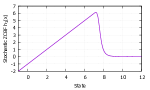
(a) The shape of $h_{1}(x)$ with $\alpha=1$ and $N=7$.

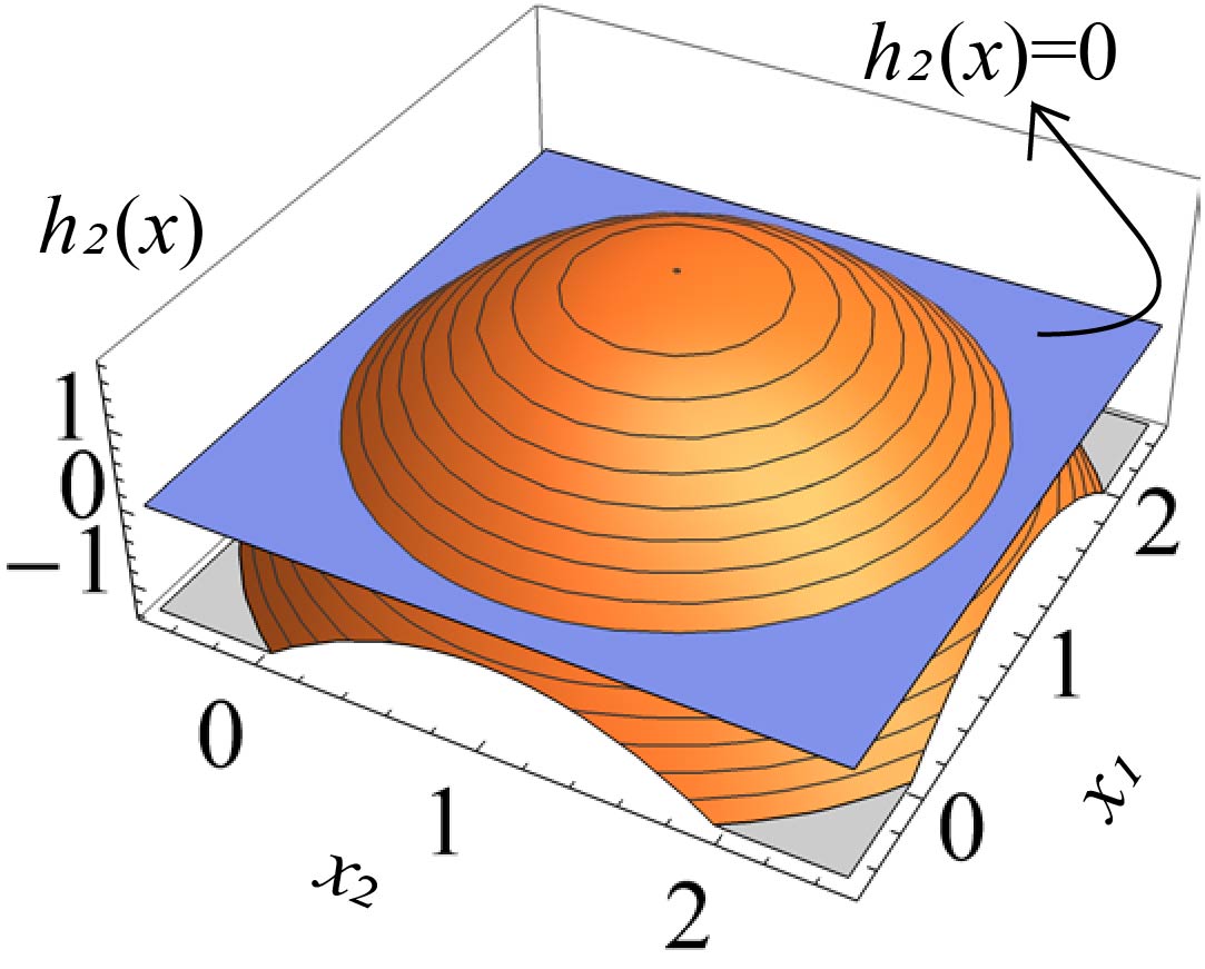
(b) The shape of $h_{2}(x)$ for $x_{3}=0$ with $P$ being the identity matrix, $\alpha_{1}=\alpha_{2}=\alpha_{3}=1$ and $M=1.8$.

Figure 1: The shape of stochastic ZCBFs $h_{1}(x)$ and $h_{2}(x)$. The safe sets are all states for which $h_{1}(x)>0$ and $h_{2}(x)>0$, respectively. From the figures, we can see that $h_{1}(x)$ and $h_{2}(x)$ are proper, respectively.

are proper in $\chi_{1}$. The shape of $h_{1}(x)$ is shown in Fig. 1.

Here, we consider $u=\phi_{N}(x)$ defined in Corollary 1. If $x\geq N$, $\phi_{N}$ is somewhat complicated because $p_{N}(x)=(x-N)^{4}$. However, if $x<N$, the calculation results in Section 3 can be straightforwardly used because $p_{N}(x)=0$. That is, $\phi_{B_{s}}$ defined in (29) is equivalent to $\phi_{N}$ for any $x<N$. Thus, we conclude $B_{1}$ and $h_{1}$ are an AS-RCBF and an AS-ZCBF, respectively.

Next, we consider the same problem setting as above, provided that the amplitude of the input is bounded; that is, for some $U_{M}>0$, an extra condition $-U_{M}\leq u_{o}(x)+u\leq U_{M}$ is considered. Setting

$$J_{2}(x):=-\gamma h_{s}(x)+c^{2}B_{s}(x),$$ (59)

let a compensator $u=\phi_{1}(x)$ by designing

$$\phi_{1}(x):=\left\{\begin{array}[]{ll}-u_{o}(x)+U_{M},&h_{s}\leq 0\cup(\max(u_{o},J_{2},U_{M})\neq U_{M}\cup J_{2}>U_{M})\\ -u_{o}(x)-U_{M},&h_{s}>0\cap(\max(u_{o},J_{2},-U_{M})=-U_{M}\cup J_{2}<-U_{M})\\ -u_{o}(x)+J_{2}(x),&h_{s}>0\cap u_{o}<J_{2}\in(-U_{M},U_{M})\\ 0,&\mathrm{otherwise}\end{array}\right.$$ (64)

and $h_{1}$ be considered as a candidate of a stochastic ZCBF. Moreover, we design

$$h(x_{\mu_{1}})=\frac{-U_{M}+\sqrt{U_{M}^{2}+4\gamma c^{2}}}{2\gamma}=:\mu_{1},$$ (65)

$$N>\frac{U_{M}+\sqrt{U_{M}^{2}+4\gamma c^{2}}}{2\gamma}=:D,$$ (66)

so that $u_{o}(x)+\phi_{1}(x)=U_{M}$ for any $x\leq x_{\mu_{1}}$ with $x_{\mu_{1}}\in(\alpha,N)$ and $u_{o}(x)+\phi_{1}(x)=-U_{M}$ for any $x\geq D$ with $N>D$.

For $x\leq x_{\mu_{1}}<N$, we obtain

$$P_{N}(x)={\dfrac{\partial{P_{N}}}{\partial{x}}}(x)={\dfrac{\partial{{}^{2}P_{N}}}{\partial{x^{2}}}}(x)=0,$$ (67)

$${\mathrm{L}_{c}{h_{1}}}(x)={\mathrm{L}_{c}{h_{s}}}(x)=c,$$ (68)

$${\mathcal{L}_{0,1,c}}(\phi_{1}(x),u_{o}(x),h_{1}(x))=\phi_{1}(x)+u_{o}(x)=U_{M};$$ (69)

thus, we obtain

$${\mathcal{L}_{0,1,c}}(\phi_{1}(x),u_{o}(x),h_{1})\geq bH_{c}(h_{1}(x))$$ (70)

with $b=2U_{M}/c^{2}$ and

$${\mathcal{L}_{0,1,c}}(\phi_{1}(x),u_{o}(x),h_{1})>bH_{c}(h_{1}(x))$$ (71)

with $b=2U_{M}/c^{2}+\epsilon$.

The above results imply that $h_{1}$ is a stochastic ZCBF and the system is safe in $(\chi_{\geq\mu_{1}},\chi,1-e^{-2U_{M}\mu_{1}/c^{2}})$, where $\chi_{\geq\mu_{1}}=\{x\in{\mathbb{R}}^{n}|h(x)\geq\mu_{1}\}$. In addition, the condition in Corollary 2 holds with $b=2U_{M}/c^{2}+\epsilon$.

Furthermore, suppose that the system (19) is nothing but a system for designing a compensator and a system

$$d{X_{t}}=(u+u_{o}({X_{t}}))dt+c^{\prime}d{W_{t}}$$ (72)

is the actual target system. If there exists $a\in[0,1]$ such that $c^{\prime}=ac$, then the system (72) is safe in $(\chi_{\geq\mu_{1}},\chi,1-e^{\frac{-2U_{M}\mu_{1}}{a^{2}c^{2}}})$. Therefore, by designing the compensator using $c>c^{\prime}$, we can make the probability of safety of $\chi_{1}$ higher, provided that it is limited by the input constraint $U_{M}$. Of course, if $a=0$, the probability is $1$.

5.2 Confinement in a bounded subset

In this subsection, we consider a stochastic nonlinear system

$$dX_{t}=\sum_{j=1}^{2}g_{j}(X_{t})(u_{oj}(X_{t})+u_{j}(t))dt+GdW_{t},\ j=1,2,$$ (73)

where

$$g_{1}(x)=\begin{bmatrix}1\\ 0\\ x_{2}\end{bmatrix},\ g_{2}(x)=\begin{bmatrix}0\\ 1\\ 0\end{bmatrix},G=\begin{bmatrix}c_{1}\\ 0\\ c_{2}\end{bmatrix},\ c_{1},c_{2}\in{\mathbb{R}}.$$ (74)

If $G=0$, the system is said to be a chained system, which is a typical model appearing in various real nonholonomic systems such as a two-wheeled vehicle robot [21].

Let a candidate of a stochastic ZCBF $h_{2}$ and a safe set $\chi_{2}$ by

$$h_{2}(x)=M-z^{T}Pz,\ z=(x_{1}-\alpha_{1},\ x_{2}-\alpha_{2},\ x_{3}-\alpha_{3})^{T},$$ (75)

$$\chi_{2}=\{x\in{\mathbb{R}}^{3}|h_{2}(x)>0\},$$ (76)

where $\alpha_{1},\alpha_{2},\alpha_{3}\in{\mathbb{R}}$, $M>0$ and $P\in{\mathbb{R}}^{3\times 3}$ is a positive definite and symmetric matrix. Note that, $z^{T}Pz$ in $h_{2}(x)$ is a control Lyapunov candidate function. Then, setting a parameter $b_{2}>0$, if ${\mathrm{L}_{g}{h_{2}}}(x)\neq 0$ and $\mathcal{L}_{0,g,G}(0,u_{o}(x),h_{2}(x))<b_{2}H_{G}(h_{2}(x))$, we design $\Phi_{2}(x)$ by

$$\Phi_{2}(x)=-u_{o}(x)-\frac{L^{I}_{G}(h_{2}(x))-b_{2}H_{G}(h_{2}(x))}{{\mathrm{L}_{g}{h_{2}}}(x)({\mathrm{L}_{g}{h_{2}}}(x))^{T}}({\mathrm{L}_{g}{h_{2}}}(x))^{T},$$ (77)

otherwise, $\Phi_{2}(x)=0$. Notice here that $\Phi_{2}$ diverges at $z=0$. However, our sufficient condition (3) for the stochastic ZCBF shows that $u$ for $x\in\chi_{h_{2}>\mu_{2}}:=\{x\in{\mathbb{R}}^{3}|h(x)>\mu_{2}\}$, where $\mu_{2}\in(0,M)$, can be anything as long as it does not lose continuity. Therefore, we design $u=\phi_{2}(x)$ by

$$\phi_{2}(x):=\left\{\begin{array}[]{ll}\Phi_{2}(x),&h(x)\leq\mu_{2},\\ \Phi_{2}(x)\frac{h_{2}(x)-M^{\prime}}{\mu-M^{\prime}},&h(x)\in(\mu_{2},M^{\prime}),\\ 0,&h(x)\geq M^{\prime},\end{array}\right.$$ (81)

where $M^{\prime}\in(\mu,M)$ and $\mu_{2}$ is designed so that $|\Phi_{2j}(x)|\leq U_{2j}$ is satisfied for all $x\in\{x\in{\mathbb{R}}^{3}|h(x)=\mu_{2}\}$ and $j=1,2$.

Applying the safety-critical control $u=\phi_{2}(x)$ to the system (73), we obtain (45) with $b=b_{2}$. Therefore, we conclude that the resulting system is safe in $(\chi_{h_{2}>\mu_{2}},\chi_{2},1-e^{-b_{2}\mu_{2}})$.

5.3 Numerical simulation

In this subsection, we confirm the validity of the derived compensators for $\chi_{1}$ and $\chi_{2}$ by computer simulation.

Example 1

Consider the system (19) with the safe set $\chi_{1}$ and the compensator $u=\phi_{1}$ discussed in Subsection 5.1. Letting $\alpha=1$, $\gamma=1$, $c=0.1$ and $U_{M}=1$, we obtain $x_{\mu_{1}}\approx 1.01$, $\mu_{1}\approx 0.01$, $b_{1}\approx 200$ and $D\approx 1.01$. The value of $N$ does not affect computer simulation if we design it massively; for example, we set $N=10^{10}$. Then, the system (19) is safe in $(\{x>x_{\mu_{1}}\},\{x>1\},0.862)$. If $u_{o}=0$ for any $t\geq 0$, the compensator $\phi_{1}$ is illustrated as in Fig. 2. Here, assuming $u_{o}=-1$ and $x_{0}=4$, the simulation results of time responses of the state $x$, the compensator $u$ and the pre-input $u_{o}$, and the ZCBF $h_{1}$ are described in Figs. 2, 2 and 2, respectively. In the simulation, we calculate ten times sample paths in the grey lines, the average of the paths in the red line, the results for the deterministic system (i.e., $\sigma^{\prime}=0$ ) in the blue line, and the pre-input $u_{o}$ in the green line.

Example 2

Consider the system (73) with the safe set $\chi_{2}$ and the compensator $u=\phi_{2}$ discussed in Subsection 5.2. Letting $c_{1}=c_{2}=0.3$, $\alpha_{1}=\alpha_{2}=\alpha_{3}=1$, $M=1.8$, $b_{2}=1$ and $\mu_{2}=1.23$, the system (73) is safe in $(\chi_{\geq\mu_{2}},\chi_{2},0.71)$. Here, assuming $u_{o}=(-x_{1},-(2x_{1}+1)x_{2}+2x_{3})^{T}$ and $x_{0}=(0.5,0.5,0.2)^{T}$, the simulation results of trajectories of $x$ is shown in Fig.3, the time responses of the compensators $u_{1}$ and $u_{2}$ are described in Figs. 3 and 3, respectively, and the time responses of the ZCBF $h_{2}$ are described in Fig. 3. The colors of the lines have the same roles as in Example 1. In Figs. 3, the stochastic ZCBF is below zero in one out of ten cases, which is a reasonable result given that the safety probability is $71$%.

In the simulation results, the safety is achieved better than the estimation of Theorem 4; note that the theorem ensures the minimum probability of leaving safe sets. The results may imply that, for actual control problems influenced by white noises, the designed compensators have good performances as safety-critical control.

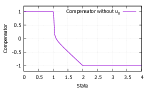
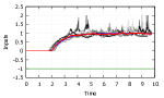
(a) The shape of the continuous state-feedback $\phi_{1}$ with $u_{o}=0$.	(b) Time responses of $x$.
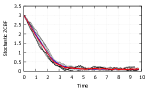
(c) Time responses of $\phi_{1}$ and $u_{o}$.	(d) Time responses of $h_{1}$.

Figure 2: Simulation results of Ex. 1. The grey colored lines denote 10 sample paths, the red colored lines denote the average of the paths, the blue lines denote the results for the deterministic system (i.e., $\sigma^{\prime}=0$ ), and the green line denote the pre-input $u_{o}(x)$. Fig. 2 shows that the safety condition $h_{1}(x)>0$ is satisfied in all 10 trials while the probability of the safety is $0.862$.

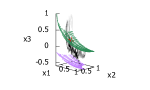
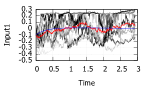
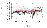
(a) The trajectories of $x$.	(b) Time responses of $u_{1}$.
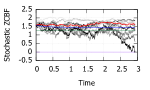
(c) Time responses of $u_{2}$.	(d) Time responses of $h_{2}(x)$.

Figure 3: Simulation results of Ex. 2. The grey, red and blue lines are used in the same way as in Fig. 2. The purple and the green lines in Figs. 3 and 3 are the boundaries of the safe set $\chi_{2}$ and the initial state sets $\chi_{\geq\mu_{2}}$, respectively. Figs. 3 and 3 show that the safety condition $h_{2}(x)>0$ is satisfied in 9 of the 10 trials while the probability of the safety is $0.71$.

6 Concluding Remarks

In this paper, we proposed an almost sure reciprocal/zeroing control barrier function and a stochastic zeroing control barrier function for designing a safety-critical control law for a stochastic control system. To demonstrate the usefulness of the proposed method, we show that stochastic ZCBFs in a problem setting such as Example 2 may be obtained based on control Lyapunov candidate functions. Because the target system is an input-affine stochastic system, the results can be extended to more general nonlinear control systems using, for example, the strategy of adding an integrator [20]. We also notice that the results are now effective for just an autonomous system with a state-feedback-type pre-input. The extension to a non-autonomous system with a time-varying pre-input is challenging for future work because the extension will enable us to apply our results for recent control application problems such as human-assist control [4, 5, 6]. Also, relaxing the constant that appears in the conditions for almost sure reciprocal/zeroing control barrier functions to the class $K_{\infty}$ function is essential, however, the relaxation requires rediscussing the existence of the solution and will be a topic for future work. In addition, since the proposed method relaxes the conditions for the existence of solutions in continuous-time stochastic systems, sensitive discussions are needed to allow for discontinuous inputs, discontinuous dynamic variations, or more complex stochastic signals. Therefore, modifying the proposed method to support digital inputs, hybrid systems, and Poisson processes is a critical future task for its practical application.

Appendix A Appendix: Proofs

A.1 Proof of Theorem 2

Applying the given condition (34) and (Z1)–(Z3) to Theorem 1, the system (2) is ensured to be FIiP in $\chi$.

A.2 Proof of Theorem 3

First, the condition (3) is transformed into

$$L^{D}_{f,g}(\phi(x),u_{o}(x),h(x))\geq-\gamma h(x)+(h(x))^{2}L^{I}_{\sigma}(B(x)).$$ (82)

Using (7) with $v=B$ and $M=\chi=\{x\in{\mathbb{R}}^{n}|h(x)>0\}$, the inequality is further transformed into

$$-(B(x))^{-2}L^{D}_{f,g}(\phi(x),u_{o}(x),B(x))\geq -\gamma(B(x))^{-1}$$

$$+(B(x))^{-2}L^{I}_{\sigma}(B)$$ (83)

for $x\in M$. Thus, we obtain

$$-(B(x))^{-2}\mathcal{L}_{f,g,\sigma}(\phi(x),u_{o}(x),B(x))\geq-\gamma(B(x))^{-1},$$ (84)

which results in (34). Therefore, the existence of an AS-ZCBF $B(x)$ ensures the system (2) is FIiP in $\chi$ via Theorem 2.

A.3 Proof of Corollary 1

First, we consider the case of ${\mathrm{L}_{g}{h}}\neq 0$. If $I<J$, we obtain

$$\mathcal{L}_{f,g,\sigma} (\phi_{N}(x),u_{o}(x),h(x))$$

$$=-\gamma h(x)+(h(x))^{2}L^{I}_{\sigma}(B(x))+L^{I}_{\sigma}(h(x)),$$ (85)

and if $I\geq J$, we obtain

$$\mathcal{L}_{f,g,\sigma} (\phi_{N}(x),u_{o}(x),h(x))=I(u_{o}(x),h(x))+L^{I}_{\sigma}(h(x))$$

$$\geq-\gamma h(x)+(h(x))^{2}L^{I}_{\sigma}(B(x))+L^{I}_{\sigma}(h(x)).$$ (86)

Therefore, regardless of $I<J$ or $I\geq J$, the inequality (3) is satisfied.

Then, we consider the other case, i.e., ${\mathrm{L}_{g}{h}}=0$. The additional condition (41) implies that there exists a sufficiently small constant $\epsilon>0$ such that

$${\mathrm{L}_{f}{h}}(x)-\epsilon\geq-\gamma h(x)+(h(x))^{2}L^{I}_{\sigma}(B(x))$$ (87)

is satisfied. Combining the inequality and the assumption of $u_{o}$ to be continuous, for a subset $G_{o}\subset\chi$, which is a neighborhood of $x_{g}\in\{x\in{\mathbb{R}}^{n}|{\mathrm{L}_{g}{h}}(x)=0\}$,

$$||{\mathrm{L}_{g}{h}}(x)u_{o}(x)||\leq\epsilon$$ (88)

is satisfied. Thus, for $x\in G_{o}$, we obtain

$${\mathrm{L}_{f}{h}}(x)+{\mathrm{L}_{g}{h}}(x)u_{o}(x)\geq-\gamma h(x)+(h(x))^{2}L^{I}_{\sigma}(B(x)),$$ (89)

which implies that $I\geq J$; namely, $\phi_{N}=0$ in $G_{o}$. Therefore, $\phi_{N}$ is continuous around ${\mathrm{L}_{g}{h}}(x)=0$.

Consequently, $\phi_{N}$ is always continuous in $\chi$ and satisfies all the assumptions and conditions of Theorem 3. This completes the proof.

A.4 Proof of Lemma 1

First, we prove that the existence of a stochastic ZCBF $h(x)$ ensures that the system (2) with $u=\phi(x)$ is FCiP. Let

$$h_{b}(x):=e^{bh(x)}.$$ (90)

Because

$$L^{D}_{f,g}(\phi(x),u_{o}(x),h_{b}(x))=bh_{b}(x)L^{D}_{f,g}(\phi,u_{o}(x),h(x)),$$ (91)

is satisfied, (45) changes as follows:

$$L^{D}_{f,g}(\phi(x),u_{o}(x),h_{b}(x))\geq bh_{b}(x)\left\{bH_{\sigma}(h(x))-L^{I}_{\sigma}(h(x))\right\}.$$ (92)

Moreover, letting

$$B_{b}(x):=(h_{b}(x))^{-1}=e^{-bh(x)},$$ (93)

we obtain

$$L^{I}_{\sigma}(B_{b}(x))=bB_{b}(x)\left\{bH_{\sigma}(h(x))-L^{I}_{\sigma}(h(x))\right\},$$ (94)

which transforms (92) into

$$L^{D}_{f,g}(\phi,u_{o}(x),h_{b}(x))\geq(h_{b}(x))^{2}L^{I}_{\sigma}(B_{b}(x)).$$ (95)

Therefore, remembering (7) with $v=B_{b}$, we obtain

$$-L^{D}_{f,g}(\phi,u_{o}(x),B_{b}(x))\geq L^{I}_{\sigma}(B_{b}(x));$$ (96)

that is,

$$\mathcal{L}_{f,g,\sigma}(\phi,u_{o}(x),B_{b}(x))\leq 0,\ x\in{\mathbb{R}}^{n}_{h\leq\mu}.$$ (97)

Here, we consider the rest space $\chi_{h>\mu}$, where the assumption (Z2)’ implies that the space is bounded and $h$ is bounded from above in the space. In addition, $B_{b}$ is decreasing, $u_{o}$ is continuous, and $f$, $g$, and $\sigma$ are all locally Lipschitz. Therefore, $\mathcal{L}_{f,g,\sigma}(\phi,u_{o}(x),B_{b}(x))$ is bounded from above; that is, for sufficiently large values $c_{1}>0$ and $c_{2}>0$, we obtain

$$\mathcal{L}_{f,g,\sigma}(\phi,u_{o}(x),B_{b}(x))\leq c_{1}B_{b}(x)+c_{2},\ x\in\chi_{h>\mu}.$$ (98)

Considering (97) and (98), all the conditions of Theorem 1 are satisfied with $Y=B_{b}$; that is, the system (2) with $u=\phi(x)$ is FCiP.

Next, going back to (97) and applying Dynkin’s formula [16, 17, 18], provided that we restrict $x_{0}\in\chi_{\mu}$, we obtain

$${\mathbb{E}\left[{B_{b}(X_{t\wedge\tau_{0\mu}})}\right]}-B_{b}(x_{0})$$

$$=\mathbb{E}\Biggl{[}\int_{0}^{t\wedge\tau_{0\mu}}\mathcal{L}_{f,g,\sigma}(\phi(X_{\tau}),u_{o}(X_{\tau}),B_{b}(X_{\tau})d\tau\Biggr{]}\leq 0.$$ (99)

Further considering Markov inequality [16, 17, 18], which is represented by

$${\mathbb{P}_{x_{0}}\left[{B_{b}(X_{\tau^{\prime}})\geq m}\right]}\leq\frac{{\mathbb{E}\left[{B_{b}(X_{\tau^{\prime}})}\right]}}{m}$$ (100)

for any stopping time $\tau^{\prime}\geq 0$ with $x\in{\mathbb{R}}^{n}$ and $m>0$, we obtain

$${\mathbb{P}_{x_{0}}\left[{B_{b}(X_{t\wedge\tau_{0\mu}})\geq m}\right]}\leq\frac{B_{b}(x_{0})}{m}.$$ (101)

Thus, choosing $m=1$ for $x_{0}\in\chi_{\mu}$, we obtain

$${\mathbb{P}_{x_{0}}\left[{h(X_{t\wedge\tau_{0\mu}})\leq 0}\right]} ={\mathbb{P}_{x_{0}}\left[{B_{b}(X_{t\wedge\tau_{0\mu}})\geq 1}\right]}$$

$$\leq B_{b}(x_{0})=e^{-bh(x_{0})}.$$ (102)

This completes the proof.

A.5 Proof of Theorem 4

Let us assume that the initial condition satisfies $x_{0}\in\chi_{h>\mu}$. Because the subset $\chi_{h>\mu}$ is bounded, any sample path $X_{t}$ has to achieve the boundary if it leaves the subset. Moreover, because $f$, $g$ and $\sigma$ of the system (2) are all time-invariant, any solution $x(t)$ is memoryless. These results imply that

$${\mathbb{P}\left[{h(X_{t\wedge\tau_{0}})\leq 0|X_{0}=x_{0}\in\chi_{h>\mu}}\right]}$$

$$\leq{\mathbb{P}\left[{h(X_{t\wedge\tau_{0}})\leq 0|X_{0}=x_{0}\in\chi_{\mu}}\right]}$$

$$\leq{\mathbb{P}\left[{h(X_{t\wedge\tau_{0\mu}})\leq 0|X_{0}=x_{0}\in\chi_{\mu}}\right]}$$ (103)

Therefore, we obtain

$${\mathbb{P}\left[{h(X_{t\wedge\tau_{0}})\leq 0|X_{0}=x_{0}\in\chi_{h>\mu}}\right]}\leq e^{-b\mu}.$$ (104)

A.6 Proof of Corollary 2

Because the condition (50) holds, for any $x\in{\mathbb{R}}^{n}_{h\leq\mu}$, $B_{b}(x)=e^{-bh(x)}$ satisfies $\mu_{b}\leq B_{b}(x)$. Using the inequality, we obtain

$$\mathcal{L}_{f,g,\sigma}(\phi,u_{o}(x),B_{b}(x))<0,\ x\in{\mathbb{R}}^{n}_{h\leq\mu}$$ (105)

via the same way to derive (97). Therefore, using Dynkin’s formula, we obtain

$$\frac{dV}{dt} =2[{\mathbb{E}\left[{B_{b}(X_{t})}\right]}-\mu_{b}]_{+}\frac{d{\mathbb{E}\left[{B_{b}(X_{t})}\right]}}{dt}$$

$$=2[{\mathbb{E}\left[{B_{b}(X_{t})}\right]}-\mu_{b}]_{+}{\mathbb{E}\left[{\mathcal{L}_{f,g,\sigma}(\phi(X_{t}),u_{o}(X_{t}),B_{b}(X_{t}))}\right]}$$

$$<0.$$ (106)

This completes the proof.

A.7 Proof of Corollary 3

By the condition (3) in Theorem 3,

$$L^{D}_{f,g}(\phi(x),u_{o}(x),h(x))\geq-\gamma h(x)+(h(x))^{2}L^{I}_{\sigma}(B(x))$$ (107)

is satisfied. Thus, we obtain

$$\mathcal{L}_{f,g,\sigma^{\prime}} (\phi(x),u_{o}(x),h(x))\geq-\gamma h(x)$$

$$+(h(x))^{2}L^{I}_{\sigma}(B(x))+L^{I}_{\sigma^{\prime}}(h(x)).$$ (108)

Here, assuming that the condition (53) holds, then we also obtain

$$\mathcal{L}_{f,g,\sigma^{\prime}} (\phi(x),u_{o}(x),h(x))\geq-\gamma h(x)$$

$$+(h(x))^{2}L^{I}_{\sigma^{\prime}}(B(x))+L^{I}_{\sigma^{\prime}}(h(x)),$$ (109)

which is the same as the condition (3), provided that $\sigma$ is replaced by $\sigma^{\prime}$. Therefore, the corollary is proven by using Theorem 3.

A.8 Proof of Corollary 4

Considering $u=\phi(x)$ and (45), we obtain

$$\mathcal{L}_{f,g,\sigma^{\prime}} (\phi(x),u_{o}(x),h(x))$$

$$=\mathcal{L}_{f,g,\sigma}(\phi(x),u_{o}(x),h(x))+L^{I}_{\sigma^{\prime}}(h(x))-L^{I}_{\sigma}(h(x))$$

$$\geq bH_{\sigma}(h(x))$$ (110)

$$\geq\frac{b}{a^{2}}H_{\sigma^{\prime}}(h(x))$$ (111)

This inequality and Theorem 4 immediately proves the corollary.

References

- [1] A. D. Ames, X. Xu, J. W. Grizzle, P. Tabuada, “Control barrier function based quadratic programs for safety critical systems,” IEEE Trans. Autom. Control, vol. 62, no. 8, pp. 3861–3876, Aug. 2017.
- [2] A. D. Ames, S. Coogan, M. Egerstedt, G. Notomista, K. Sreenath, P. Tabuada, “Control barrier functions: theory and applications,” Proc. 18th Euro. Control Conf., pp. 3420–3431, 2019.
- [3] T. Shimizu, S. Yamashita, T. Hatanaka, K. Uto, M. Mammarella and F. Dabbene, “Angle-aware coverage control for 3-D map reconstruction with drone networks,” IEEE Control Syst. Lett., vol. 6, pp. 1831–1836, 2022.
- [4] S. Furusawa, H. Nakamura, “Human assist control considering shape of target system,” Asian J. Control, vol. 23, no. 3, pp. 1185–1194, 2021.
- [5] H. Nakamura, T. Yoshinaga, Y. Koyama, and S. Etoh, “Control barrier function based human assist control,” Trans. Society of Instrumental and Control Engineering, vol. 55, no. 5, pp. 353–361, 2019.
- [6] I. Tezuka and H. Nakamura, “Strict zeroing control barrier function for continuous safety assist control,” IEEE Control Syst. Lett., vol. 6, pp. 2108–2113, 2022.
- [7] P. Jagtap, S. Soudjani and M. Zamani, “Formal synthesis of stochastic systems via control barrier certificates,” IEEE Trans. Autom. Control, vol. 66, no. 7, pp. 3097–3110, 2021.
- [8] A. Salamati and M. Zamani, “Safety verification of stochastic systems: a repetitive scenario approach,” IEEE Control Syst. Lett., vol. 7, pp. 448–453, 2023.
- [9] S. Prajna, A. Jadbabaie and G. J. Pappas, “A framework for worst-case and stochastic safety verification using barrier certificates,” IEEE Trans. Autom. Control, vol. 52, no. 8, pp. 1415–1428, 2007.
- [10] C. Santoyo, M. Dutreix and S. Coogan, “Verification and control for finite-time safety of stochastic systems via barrier functions,” Proc. 2019 IEEE Conf. Control Tech. Appl., pp. 712–717, 2019.
- [11] R. Wisniewski and L.-M. Bujorianu, “Safety of stochastic systems: an analytic and computational approach,” Automatica, vol. 133, DOI: 10.1016/j.automatica.2021.109839, 2021.
- [12] A. Clark, “Control barrier functions for stochastic systems,” Automatica, 130, DOI: 10.106/j.automatica.2021.109688, 2021.
- [13] C. Wang, Y. Meng, S. L. Smith and J. Liu, “Safety-critical control of stochastic systems using stochastic control barrier functions,” Proc. IEEE 60th Annu. Conf. Decis. Control, pp. 5924–5931, 2021.
- [14] Y. Nishimura, “Conditions for local almost sure asymptotic stability,” Syst. Control Lett., vol. 94, pp. 19–24, 2016.
- [15] Y. Nishimura and H. Ito, “Stochastic Lyapunov functions without differentiability at supposed equilibria,” Automatica, vol. 92, no. 6, pp. 188–196, 2018.
- [16] R. Z. Khasminskii, Stochastic Stability of Differential Equations, Second Edition, Springer, 2012.
- [17] H. J. Kushner, Stochastic Stability and Control, Academic Press, 1967.
- [18] X. Mao, Stochastic Differential Equations and Applications, Second Edition, Woodhead Publishing, 2007.
- [19] A. Poznyak, “Stochastic super-twist sliding mode controller,” IEEE Trans. Autom. Control, vol. 63, no. 5, pp. 1538–1544, 2018.
- [20] J. -M. Coron, “Adding an integrator for the stabilization problem,” Syst. Control Lett., vol. 17, pp. 89–104, 1991.
- [21] A. M. Bloch. Nonholonomic Mechanics and Control Second Edition, Springer, 2015.