Dissipative magnetic structures and scales in small-scale dynamos

Abstract

Small-scale dynamos play important roles in modern astrophysics, especially on Galactic and extragalactic scales. Owing to dynamo action, purely hydrodynamic Kolmogorov turbulence hardly exists and is often replaced by hydromagnetic turbulence. Understanding the size of dissipative magnetic structures is important in estimating the time scale of Galactic scintillation and other observational and theoretical aspects of interstellar and intergalactic small-scale dynamos. Here we show that, during the kinematic phase of the small-scale dynamo, the cutoff wavenumber of the magnetic energy spectra scales as expected for large magnetic Prandtl numbers, but continues in the same way also for moderately small values – contrary to what is expected. For a critical magnetic Prandtl number of about 0.3, the dissipative and resistive cutoffs are found to occur at the same wavenumber. In the nonlinearly saturated regime, the critical magnetic Prandtl number becomes unity. The cutoff scale now has a shallower scaling with magnetic Prandtl number below a value of about three, and a steeper one otherwise compared to the kinematic regime.

1 Introduction

Since the early 1990s, we know that dissipative structures in hydrodynamic turbulence are vortex tubes (She et al., 1990; Vincent & Meneguzzi, 1991). Their typical size is of the order of the Kolmogorov length. In magnetohydrodynamics (MHD), the dissipative structures are magnetic flux tubes (Nordlund et al., 1992; Brandenburg et al., 1996; Moffatt et al., 1994; Politano & Pouquet, 1998). Their thickness has been estimated to scale with the magnetic Prandtl number $\mbox{\rm Pr}_{\rm M}=\nu/\eta$, i.e., the ratio of the kinematic viscosity $\nu$ to the magnetic diffusivity $\eta$. Brandenburg et al. (1995), hereafter BPS, estimated the typical coherence scale of magnetic field vectors in terms of the gradient matrix ${\bm{\nabla}}\hat{\bm{B}}$ of the unit vector $\hat{\bm{B}}=\bm{B}/|\bm{B}|$ of the magnetic field $\bm{B}$ and found that it scales like $\mbox{\rm Pr}_{\rm M}^{-1/2}$ relative to the Kolmogorov length scale. The inverse length scale of the magnetic structures can be calculated as the rms value of ${\bm{\nabla}}\hat{\bm{B}}$, i.e., $k_{B}=\langle|{\bm{\nabla}}\hat{\bm{B}}|^{2}\rangle^{1/2}$. The simulations of BPS were for the case of a convection-driven dynamo in the presence of rotation and compressibility, but similar results were later also obtained by Schekochihin et al. (2004) for a small-scale dynamo in homogeneous incompressible turbulence for $\mbox{\rm Pr}_{\rm M}\leq 1$. They also emphasized that a steeper dependence on $\mbox{\rm Pr}_{\rm M}$ is expected for $\mbox{\rm Pr}_{\rm M}\ll 1$.

The mechanisms of the small-scale dynamo action are different depending on the magnetic Prandtl number. For $\mbox{\rm Pr}_{\rm M}\gg 1$, self-excitation of magnetic fluctuations is caused by the random stretching of the magnetic field by a smooth velocity field; see the analytical studies by Kazantsev (1968), Zeldovich et al. (1990), Kulsrud & Anderson (1992, hereafter KA), and Schober et al. (2012). For $\mbox{\rm Pr}_{\rm M}\ll 1$, the small-scale dynamo is driven by velocity fluctuations at the resistive scale, which is located in the inertial range (Kazantsev, 1968; Rogachevskii & Kleeorin, 1997; Boldyrev & Cattaneo, 2004; Arponen & Horvai, 2007; Kleeorin & Rogachevskii, 2012; Martins Afonso et al., 2019). In particular, KA found that, for large values of $\mbox{\rm Pr}_{\rm M}$, the magnetic energy spectrum is expected to be of the form

$$E_{\rm M}(k,t)\propto e^{2\gamma t}k^{3/2}K_{0}\left(k/k_{\eta}^{\rm KA}\right),$$ (1)

where $K_{0}$ is the Macdonald function of order zero (or the modified Bessel function of the second kind), and $k_{\eta}^{\rm KA}$ is

$$k_{\eta}^{\rm KA}=(4\gamma/15\eta)^{1/2},$$ (2)

where $\gamma$ is the growth rate of the magnetic field. This provides another very different method for calculating a relevant wavenumber characterizing the scale of structures than $k_{B}$.

The question of characteristic length scales in a small-scale dynamo continued attracting attention and has been investigated in more detail by Cho & Ryu (2009) with applications to the intergalactic medium. Much of this work concerns the saturated phase of the dynamo, but Eq. (1) is then not applicable. More recently, Kriel et al. (2022) confirmed the $\mbox{\rm Pr}_{\rm M}^{-1/2}$ scaling for $1\leq\mbox{\rm Pr}_{\rm M}\leq 260$ for the kinematic phase of the dynamo. The small-scale properties of interstellar turbulence can be assessed through interstellar scintillation measurements of pulsars (Cordes et al., 1985; Rickett, 1990; Armstrong et al., 1995; Bhat et al., 2004; Scalo & Elmegreen, 2004). A particular difficulty is to explain what is known as extreme scattering events (ESEs), which would require unrealistically large pressures if the scattering structures were spherical (Clegg et al., 1998). This favors the presence of sheet- or tube-like structures that could explain ESEs of those structures are oriented along the line-of-sight (Pen & King, 2012; Bannister et al., 2016). Scintillation measurements suggest that the dissipative structures of MHD turbulence are sheet-like with an inner scale down to $300\,{\rm km}$ (Bhat et al., 2004). However, more detailed measurements would be needed to determine the precise nature of the smallest dissipative structures (Xu & Zhang, 2017).

The goal of the present paper is to compare the relations between different length scales in small-scale dynamos. We mainly focus here on the kinematic growth phase of the dynamo, but we also consider some nonlinear models in Sects. 3.1 and 3.6. In addition to the values of $k_{\eta}^{\rm KA}$ and $k_{B}$ discussed above, we also determine a wavenumber $k_{\eta}$ that describes the resistive cutoff of the spectrum, and is analogous to the wavenumber $k_{\nu}$ based on the Kolmogorov (viscous) scale. Kriel et al. (2022) used a similar prescription, but did not compare with other magnetic scales. Note that, contrary to $k_{\eta}^{\rm KA}$, $k_{\eta}$ is not calculated from the dynamo growth rate. Following earlier work (Brandenburg et al., 2018), we consider weakly compressible turbulence with an isothermal equation of state and a constant sound speed $c_{\rm s}$, where the pressure is proportional to the density $\rho$, i.e., $p=\rho c_{\rm s}^{2}$.

2 The model

2.1 Basic equations

In this work, we are primarily interested in weak magnetic fields and ignore therefore the Lorentz force in most simulations. The magnetic field is given as $\bm{B}={\bm{\nabla}}\times\bm{A}$, where $\bm{A}$ is the magnetic vector potential. We thus solve the evolution equations for the magnetic vector potential $\bm{A}$, the velocity $\bm{u}$, and the logarithmic density $\ln\rho$ in the form

$$\frac{\partial\bm{A}}{\partial t}=\bm{u}\times\bm{B}+\eta\nabla^{2}\bm{A},$$ (3)

$$\frac{{\rm D}{}\bm{u}}{{\rm D}{}t}=\mbox{\boldmath$f$}{}-c_{\rm s}^{2}{\bm{\nabla}}\ln\rho+\frac{1}{\rho}{\bm{\nabla}}\cdot(2\rho\nu\mbox{\boldmath${\sf S}$}{}),$$ (4)

$$\frac{{\rm D}{}\ln\rho}{{\rm D}{}t}=-{\bm{\nabla}}\cdot\bm{u},$$ (5)

where ${\rm D}{}/{\rm D}{}t=\partial/\partial t+\bm{u}\cdot{\bm{\nabla}}$ is the advective derivative, $f$ is a nonhelical forcing function consisting of plane waves with wavevector $\bm{k}$, and ${\sf S}_{ij}=(\partial_{i}u_{j}+\partial_{j}u_{i})/2-\delta_{ij}{\bm{\nabla}}\cdot\bm{u}/3$ are the components of the rate-of-strain tensor ${\sf S}$. For the forcing, we select a $\bm{k}$ vector at each time step randomly from a finite shell around $k_{\rm f}/k_{1}=1.5$ with $1\leq|\bm{k}|/k_{1}<2$. The components of $\bm{k}$ are taken to be integer multiples of $k_{1}\equiv 2\pi/L$, where $L$ is the side length of our Cartesian domain of volume $L^{3}$. This forcing function has been used in many earlier papers (e.g. Haugen et al., 2004). We solve Eqs. (3)–(5) using the Pencil Code (Pencil Code Collaboration et al., 2021).

2.2 Spectra and characteristic parameters

We normalize our kinetic and magnetic energy spectra such that $\int E_{\rm K}(k)\,{\rm d}{}k=\langle\bm{u}^{2}\rangle/2$ and $\int E_{\rm M}(k)\,{\rm d}{}k=\langle\bm{B}^{2}\rangle/2\mu_{0}\rho_{0}\equiv{\cal E}_{\rm M}$, respectively, where $\rho_{0}$ is the mean density. Here, angle brackets without subscript denote volume averages. We always present time-averaged spectra. Since $E_{\rm M}(k,t)$ increases exponentially at the rate $2\gamma$, where $\gamma$ is the growth rate of the magnetic field, we average the compensated spectra, $\langle e^{-2\gamma t}E_{\rm M}(k,t)\rangle_{\Delta t}$, over a suitable time interval $\Delta t$ where the function $e^{-2\gamma t}E_{\rm M}(k,t)$ is statistically stationary; see also Subramanian & Brandenburg (2014). Our averaged magnetic energy spectra are normalized by ${\cal E}_{\rm M}$, so that their integral is unity.

Our governing parameters are the Mach number, and the fluid and magnetic Reynolds numbers, defined here as

$$\mbox{\rm Ma}=u_{\rm rms}/c_{\rm s},\quad\mbox{\rm Re}=u_{\rm rms}/\nu k_{\rm f},\quad\mbox{\rm Re}_{\rm M}=u_{\rm rms}/\eta k_{\rm f},$$ (6)

respectively, where $u_{\rm rms}$ is the time-averaged rms velocity. Thus, the magnetic Prandtl number is $\mbox{\rm Pr}_{\rm M}=\mbox{\rm Re}_{\rm M}/\mbox{\rm Re}$. The value of $\gamma$ is computed as the average of ${\rm d}{}\ln B_{\rm rms}/{\rm d}{}t$ during the exponential growth phase. We also give the kinetic dissipation wavenumber

$$k_{\nu}=\left(\epsilon_{\rm K}/\rho_{0}\nu^{3}\right)^{1/4},$$ (7)

where $\epsilon_{\rm K}=\langle 2\rho\nu\mbox{\boldmath${\sf S}$}{}^{2}\rangle_{\Delta t}$ is the time-averaged kinetic energy dissipation rate. It obeys the expected $\mbox{\rm Re}^{3/4}$ scaling, here with $k_{\nu}/k_{\rm f}\approx 0.48\,\mbox{\rm Re}^{3/4}$; see Appendix A.

In fluid dynamics, to avoid discussions about different definitions of the Reynolds number, one commonly quotes the Taylor microscale Reynolds number (Tennekes & Lumley, 1972), which is universally defined as $\mbox{\rm Re}_{\lambda}=u^{\prime}\lambda_{\rm Tay}/\nu$. Here, $u^{\prime}=u_{\rm rms}/\sqrt{3}$ is the one-dimensional rms velocity and $\lambda_{\rm Tay}=\sqrt{15\nu\rho_{0}/\epsilon_{\rm K}}\,u^{\prime}$ is the Taylor microscale. The values of $\mbox{\rm Re}_{\lambda}$ are given in Table 1. They are expected to be proportional to $\mbox{\rm Re}^{1/2}$, but the actual scaling is slightly steeper; see the Supplemental Material (Brandenburg et al., 2022a).

A tilde on the growth rate denotes normalization with the turnover rate and tildes on various wavenumbers denote normalization with respect to $k_{1}$, i.e.,

$$\tilde{\gamma}=\gamma\tau,\quad\tilde{k}_{\nu}=k_{\nu}/k_{1},\quad\tilde{k}_{\rm f}=k_{\rm f}/k_{1},\quad\mbox{etc},$$ (8)

where $\tau=1/u_{\rm rms}k_{\rm f}$ is the turnover time. These parameters are listed in Table 1 for our runs. For Runs A–K, we used a resolution of $512^{3}$ mesh points, while we used $1024^{3}$ mesh points for Runs L and M, and $2048^{3}$ mesh points for Run M’. The value of $\epsilon_{\rm K}$ in units of $\rho_{0}k_{1}c_{\rm s}^{3}$ is obtained from the table entries as $\epsilon_{\rm K}/\rho_{0}k_{1}c_{\rm s}^{3}=\tilde{k}_{\nu}^{4}(\mbox{\rm Ma}/\mbox{\rm Re}\,\tilde{k}_{\rm f})^{3}$. The calculation of the values of $\tilde{k}_{\eta}$ is discussed below. Error bars are computed from time series as the largest departure of any one third compared to the total.

In some cases, we examine the effects of nonlinear saturation. We then include the Lorentz force and replace Eq. (4) by

$$\frac{{\rm D}{}\bm{u}}{{\rm D}{}t}=\mbox{\boldmath$f$}{}-c_{\rm s}^{2}{\bm{\nabla}}\ln\rho+\frac{1}{\rho}\Big{[}{\bm{\nabla}}\cdot(2\rho\nu\mbox{\boldmath${\sf S}$}{})+\bm{J}\times\bm{B}\Big{]}.$$ (9)

Once the Lorentz force is included, the magnetic field is expected to saturate near the equipartition magnetic field strength, $B_{\rm eq}=\sqrt{\mu_{0}\rho_{0}}u_{\rm rms}$.

Table 1: Summary of the kinematic simulations presented in this paper.

Run	Ma	$\mbox{\rm Re}_{\lambda}$	Re	$\mbox{\rm Re}_{\rm M}$	$\mbox{\rm Pr}_{\rm M}$	$\tilde{\gamma}$	$\tilde{k}_{\nu}$	$\tilde{k}_{B}$	$\tilde{k}_{\eta}^{\rm KA}$	$\tilde{k}_{\eta}$	$\Delta t/\tau$	$N$
A	0.096	13	12	1240	100	$0.076\pm 0.014$	$5.9\pm 0.1$	$127\pm 2$	$7.7\pm 0.7$	$109\pm 4$	31	512
B	0.113	30	36	1460	40	$0.090\pm 0.006$	$11.7\pm 0.1$	$128\pm 4$	$9.1\pm 0.3$	$129\pm 4$	62	512
C	0.120	50	78	1560	20	$0.110\pm 0.002$	$19.7\pm 0.2$	$139\pm 3$	$10.4\pm 0.2$	$156\pm 6$	87	512
D	0.127	70	165	1650	10	$0.135\pm 0.006$	$34.1\pm 0.2$	$156\pm 3$	$11.8\pm 0.2$	$187\pm 8$	98	512
E	0.130	120	420	1680	4	$0.159\pm 0.007$	$68\pm 2$	$185\pm 3$	$13.0\pm 0.3$	$248\pm 10$	75	512
F	0.128	170	830	1660	2	$0.172\pm 0.014$	$113\pm 5$	$209\pm 6$	$13.4\pm 0.5$	$293\pm 15$	62	512
G	0.129	250	1670	1670	1	$0.157\pm 0.016$	$185\pm 7$	$237\pm 4$	$12.9\pm 0.6$	$358\pm 15$	43	512
G’	0.131	250	1700	1700	1	$0.144\pm 0.020$	$188\pm 10$	…	$12.5\pm 0.6$	$358\pm 15$	54	1024
H	0.132	260	1710	850	0.5	$0.079\pm 0.006$	$187\pm 6$	$147\pm 4$	$6.5\pm 0.3$	$260\pm 15$	101	512
I	0.134	260	1740	580	0.33	$0.042\pm 0.010$	$189\pm 5$	$114\pm 3$	$3.9\pm 0.5$	$216\pm 15$	78	512
J	0.130	260	1680	420	0.25	$0.029\pm 0.001$	$185\pm 3$	$92\pm 1$	$2.8\pm 0.3$	$189\pm 20$	712	512
K	0.130	250	1680	340	0.20	$0.019\pm 0.004$	$186\pm 5$	$82\pm 4$	$2.0\pm 0.2$	$168\pm 20$	99	512
L	0.132	420	4270	427	0.10	$0.020\pm 0.003$	$368\pm 10$	$107\pm 2$	$2.3\pm 0.3$	$249\pm 18$	193	1024
M	0.132	650	8300	430	0.05	$0.013\pm 0.008$	$575\pm 17$	$103\pm 4$	$1.8\pm 0.4$	$332\pm 15$	61	1024
M’	0.134	620	8700	430	0.05	$0.016\pm 0.011$	$610\pm 12$	$103\pm 4$	$1.8\pm 0.4$	$332\pm 15$	6	2048

3 Results

3.1 Growth phase of the dynamo

In most of this work, we analyze kinematic dynamo action, i.e., the Lorentz force is weak and can be neglected. This means that the magnetic field of a supercritical dynamo grows exponentially beyond any bound.

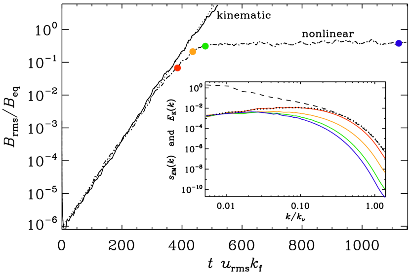
Figure 1: Nonlinear saturation (Run j of Sect. 3.6 below) compared with the kinematic evolution for Run J (see Table 1). The red, orange, green, and blue dots mark the times when $B_{\rm rms}/B_{\rm eq}\approx 0.07$, 0.2, 0.3, and 0.4. The inset shows scaled magnetic energy spectra, $s_{E}E_{\rm M}(k)$, where $s_{E}=16$, 0.45, 0.11, and 0.06, so as to make the spectra overlap near the smallest wavenumber. The dashed and dotted lines give the time-averaged spectra $E_{\rm K}(k)$ and $E_{\rm M}(k)$, respectively in the kinematic regime without the Lorentz force.

To quantify the point until when the Lorentz force can indeed be neglected, we present in this section simulations with the Lorentz force included; see Eq. (9). We then expect the magnetic field to saturate near $B_{\rm eq}$. In Fig. 1, we show the evolution of $B_{\rm rms}/B_{\rm eq}$ for cases with and without Lorentz force included. We also mark four particular times for which we also show the magnetic energy spectra in the nonlinear regime. We see that, when $B_{\rm rms}/B_{\rm eq}\approx 0.05$, the magnetic energy spectrum (red line) is still close to the time-averaged kinematic spectrum (dotted line). At the time when $B_{\rm rms}/B_{\rm eq}\approx 0.2$, we begin to see clear departures from the kinematic spectrum $E_{\rm M}(k)$. To see this more clearly, we have scaled the amplitude of the spectra such that they agree with the kinematic one (dotted line) near the smallest wavenumber. Finally, when $B_{\rm rms}/B_{\rm eq}\approx 0.3$, a slow phase of nonlinear saturation commences where the value of $B_{\rm rms}/B_{\rm eq}$ hardly changes, but the spectrum still changes in such a way that its peak moves into the inertial range. This is an important difference to the kinematic stage and was first report by Haugen et al. (2003). The final value of $B_{\rm rms}/B_{\rm eq}$ is about 0.4.

3.2 Scalings of the KA and flux tube wavenumbers

Looking at Table 1, it is clear that the inverse flux tube thickness $\tilde{k}_{B}$ does not change monotonically with $\mbox{\rm Pr}_{\rm M}$. The same is also true for $\tilde{k}_{\eta}^{\rm KA}$. This is mostly because $\mbox{\rm Re}_{\rm M}$ was not kept constant for all runs. For $\mbox{\rm Pr}_{\rm M}\geq 1$, however, $\mbox{\rm Re}_{\rm M}$ varied only little and was in the range from 1200 to 1700. In that range, $\tilde{k}_{B}$ showed a steady increase with $\mbox{\rm Pr}_{\rm M}$. For smaller $\mbox{\rm Pr}_{\rm M}$, we decrease $\mbox{\rm Re}_{\rm M}$ so that Re did not become too large. For Runs L and M, we used a resolution of $1024^{3}$ and were thus able to increase Re, which led to a slight increase of $\tilde{k}_{B}$. For Run M’, we used $2048^{3}$ mesh points and find results comparable to those of Run M, except for the larger statistical error. In most of the plots, we normalize the characteristic wavenumbers by $k_{\nu}$, which resulted in a monotonic increase of the ratios $k_{B}/k_{\nu}$ and $k_{\eta}^{\rm KA}/k_{\nu}$.

In Fig. 2, we plot $k_{\eta}^{\rm KA}/k_{\nu}$ and $k_{B}/k_{\nu}$ versus $\mbox{\rm Pr}_{\rm M}$. Both show a $\mbox{\rm Pr}_{\rm M}^{0.6}$ scaling for $\mbox{\rm Pr}_{\rm M}\geq 2$, but they have a linear dependence for $\mbox{\rm Pr}_{\rm M}<1$. Thus, the expected $\mbox{\rm Pr}_{\rm M}^{1/2}$ scaling is only approximately confirmed.

Figure 2: Dependence of $k_{\eta}^{\rm KA}/k_{\nu}$ (closed symbols) and $k_{B}/k_{\nu}$ (open symbols) on $\mbox{\rm Pr}_{\rm M}$. The dotted line shows the $\mbox{\rm Pr}_{\rm M}^{1/2}$ scaling for comparison.

3.3 Resistive cutoff wavenumbers

Important characteristics of MHD turbulence are the kinetic and magnetic energy spectra. Focussing on the viscous and resistive dissipation subranges, it makes sense to normalize $k$ by $k_{\nu}$, as discussed above. We recall that the quantity $k_{\nu}$ is usually defined as in Eq. (7), i.e., without any prefactors. The point when the spectrum drops significantly is typically at $k/k_{\nu}\approx 0.1$ rather than at unity, as one might have expected. This should be kept in mind when discussing values of cutoff wavenumbers in other definitions. We return to this at the end of the paper.

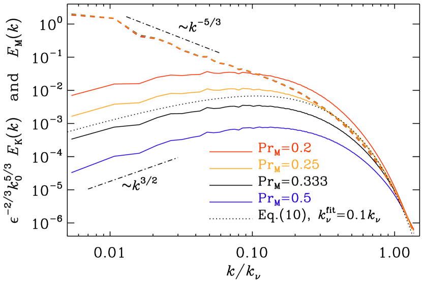
Figure 3: Magnetic energy spectra (solid lines) for $\mbox{\rm Pr}_{\rm M}=1/5$ (Run K, red), 1/4 (Run J, orange), 1/3 (Run I, black), and 1/2 (Run H, blue) along with the corresponding kinetic energy spectra (dashed lines).

The functional forms of $E_{\rm M}(k)$ and $E_{\rm K}(k)$ are rather different at small values of $k$, but near the viscous cutoff wavenumber they are more similar to each other. In Fig. 3, we compare $E_{\rm K}(k)$ and $E_{\rm M}(k)$ for a few values of $\mbox{\rm Pr}_{\rm M}$. We clearly recognize the $E_{\rm K}(k)\propto k^{-5/3}$ Kolmogorov scaling and the $E_{\rm M}(k)\propto k^{3/2}$ spectrum of the small-scale dynamo (Kazantsev, 1968); see also KA. For different values of $\mbox{\rm Pr}_{\rm M}$, however, the slopes of $E_{\rm M}(k)$ are quite different near the resistive cutoff wavenumber: steeper for small values of $\mbox{\rm Pr}_{\rm M}$ and shallower for larger values of $\mbox{\rm Pr}_{\rm M}$. For $\mbox{\rm Pr}_{\rm M}=1/4=0.25$, the shapes of $E_{\rm M}(k)$ and $E_{\rm K}(k)$ are most similar to each other at large $k$, although $E_{\rm M}(k)$ is just slightly too steep, while for $\mbox{\rm Pr}_{\rm M}\geq 1/3$, it is already clearly too shallow. Thus, we expect there to be a critical value, $\mbox{\rm Pr}_{\rm M}^{\rm crit}$ of about 0.3, where $E_{\rm M}(k)$ and $E_{\rm K}(k)$ are most similar to each other near the cutoff wavenumber.

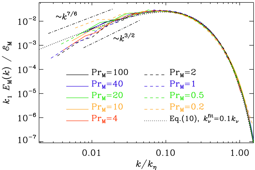
Figure 4: Magnetic energy spectra collapsed on top of each other by choosing suitable values of $k_{\eta}$ for each value of $\mbox{\rm Pr}_{\rm M}$. The dotted line shows Eq. (10) with $k_{\eta}^{\rm fit}=0.13\,k_{\eta}$.

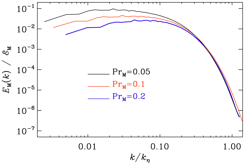
Figure 5: Similar to Fig. 4, but for $\mbox{\rm Pr}_{\rm M}=0.05$ (black line), 0.1 (red line), and 0.2 (blue line).

The spectral behavior near the resistive cutoff can be compared with Eq. (1) using an empirical fit parameter through

$$k_{1}E_{\rm M}(k)/{\cal E}_{\rm M}=A_{0}\,\left(k/k_{\eta}^{\rm fit}\right)^{3/2}K_{0}\left(k/k_{\eta}^{\rm fit}\right),$$ (10)

where $k_{\eta}^{\rm fit}$ is now treated as an adjustable parameter. In Fig. 3, we have already compared with Eq. (10), although the match is not very good. This is mostly because the model applies to large values of $\mbox{\rm Pr}_{\rm M}$, and then the fit improves, as we will see below.

By choosing suitable values of $k_{\eta}$ for $\mbox{\rm Pr}_{\rm M}\neq\mbox{\rm Pr}_{\rm M}^{\rm crit}$, we can now try to collapse the curves $E_{\rm M}(k/k_{\eta})$ on top of each other. This is done in Fig. 4, where we use Run I with $\mbox{\rm Pr}_{\rm M}=0.33$ as references run, because this value is close to $\mbox{\rm Pr}_{\rm M}^{\rm crit}$. The collapse is good near and above the peak of the spectra, but there are departures for small values of $k$, where the spectra become shallower than the classical Kazantsev slope for smaller values of $\mbox{\rm Pr}_{\rm M}$. In the opposite limit of $\mbox{\rm Pr}_{\rm M}\ll 1$, the spectral slope may be smaller. For $\mbox{\rm Pr}_{\rm M}=0.1$, a $k^{7/6}$ scaling was previously discussed by Subramanian & Brandenburg (2014) and confirmed by Brandenburg et al. (2018). For $\mbox{\rm Pr}_{\rm M}\leq 0.2$, the quality of the collapse onto Eq. (1) becomes rather poor, which is why we plot the results for smaller values separately; see Fig. 5.

The collapse for each value of $\mbox{\rm Pr}_{\rm M}$ results in a value of $k_{\eta}$, which we have listed in Table 1. A plot of $k_{\eta}/k_{\nu}$ versus $\mbox{\rm Pr}_{\rm M}$ is given in Fig. 6. We see that the ratio $k_{\eta}/k_{\nu}$ does obey the expected $\mbox{\rm Pr}_{\rm M}^{1/2}$ scaling rather well. In this figure, we have also highlighted the value of $\mbox{\rm Pr}_{\rm M}=\mbox{\rm Pr}_{\rm M}^{\rm crit}\approx 0.3$ where $k_{\eta}/k_{\nu}=1$, so

$$k_{\eta}/k_{\nu}=\left(\mbox{\rm Pr}_{\rm M}/\mbox{\rm Pr}_{\rm M}^{\rm crit}\right)^{1/2}.$$ (11)

For $\mbox{\rm Pr}_{\rm M}\ll 1$, a steeper scaling is numerically obtained at very high resolution simulations (Warnecke et al., 2022), but in our simulations, such a trend cannot yet be seen for $\mbox{\rm Pr}_{\rm M}\geq 0.05$.

Figure 6: Dependence of $k_{\eta}/k_{\nu}$ (closed symbols) on $\mbox{\rm Pr}_{\rm M}$.

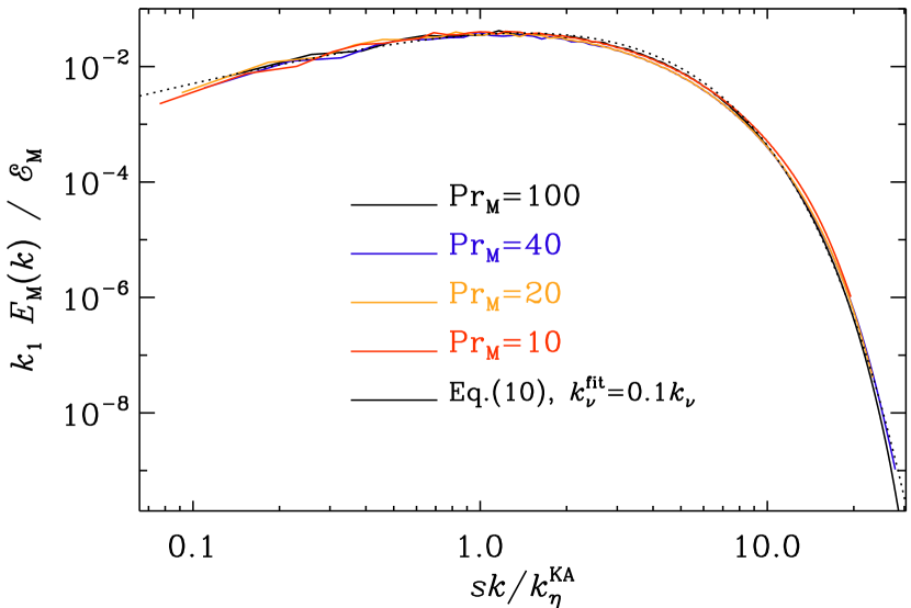
Figure 7: Magnetic energy spectra versus $k/k_{\eta}^{\rm KA}$ for $\mbox{\rm Pr}_{\rm M}=100$ (black solid line) and collapsed on top of it the result for $\mbox{\rm Pr}_{\rm M}=40$ (blue line), as well as $\mbox{\rm Pr}_{\rm M}=20$ (orange line, having scaled $k_{\eta}^{\rm KA}$ by a factor 1.05), and $\mbox{\rm Pr}_{\rm M}=10$ (red line, having scaled $k_{\eta}^{\rm KA}$ by a factor 1.1). The dotted line shows Eq. (10) with $k_{\eta}^{\rm fit}=1.32\,sk_{\eta}^{\rm KA}$.

3.4 Comparison with the Kazantsev cutoff wavenumber

We have already discussed the differences in the $\mbox{\rm Pr}_{\rm M}$ scaling between the measured $k_{\eta}$ and the theoretically expected $k_{\eta}^{\rm KA}$ from the work of KA based on the numerically determined growth rate. Here, however, the scales are rather different in an absolute sense. This is primarily caused by the large departure between the values of $k_{\eta}^{\rm KA}$ and the location where the magnetic energy spectrum begins to drop rapidly. The apparent discrepancy can be alleviated by redefining $k_{\nu}$ such that the drop occurs closer to unity. Thus, there is otherwise no physical significance in the difference of the absolute wavenumbers.

To clarify this point, we now plot $k_{1}E_{\rm M}(k)/{\cal E}_{\rm M}$ versus $k/k_{\eta}^{\rm KA}$ for $\mbox{\rm Pr}_{\rm M}=100$ and 40. For smaller values of $\mbox{\rm Pr}_{\rm M}$, we have scaled $k_{\eta}^{\rm KA}$ by a factor $s=1.05$ for $\mbox{\rm Pr}_{\rm M}=20$ and by a factor $s=1.1$ for $\mbox{\rm Pr}_{\rm M}=10$; see Fig. 7. Those coefficients are also listed in Table 2. The result for $\mbox{\rm Pr}_{\rm M}=4$ is not plotted because of a poor collapse at small $k$. Here, the adjustment factor is 1.3, as listed in Table 2. This lack of collapse for $\mbox{\rm Pr}_{\rm M}\leq 4$ illustrates that only for large values of $\mbox{\rm Pr}_{\rm M}$, the Kazantsev model reproduces the numerical data related to $k_{\eta}^{\rm KA}$ sufficiently well.

Table 2: Values of $k_{\eta}^{\rm KA}$ and adjustment factors to the KA values for $\mbox{\rm Pr}_{\rm M}\leq 20$.

$\mbox{\rm Pr}_{\rm M}$	100	40	20	10	4
$\tilde{k}_{\eta}^{\rm KA}$	7.7	9.1	10.4	11.9	13.0
$s$	1	1.00	1.05	1.1	1.3
$1.3\,s\tilde{k}_{\eta}^{\rm KA}$	10.0	11.8	14.1	16.9	21.9
$k_{\eta}^{\rm fit}/k_{\nu}$	2.87	1.44	0.56	0.38	0.25

In absolute terms, the value of $k_{\eta}^{\rm KA}$ given by Eq. (2) underestimates the position of the peak by a factor of about $1.3=1/0.77$. This factor was obtained empirically by having overplotted in Fig. 7 the graph of Eq. (10) with

$$k_{\eta}^{\rm fit}\approx 0.093\,k_{\eta}\approx 1.32\,sk_{\eta}^{\rm KA}.$$ (12)

The agreement with the numerical solutions is generally good, but deteriorates for $\mbox{\rm Pr}_{\rm M}<10$, especially for small $k$, where the simulation results predict less power than the Kazantsev model. On the other hand, the discrepancy with the estimate of $k_{\eta}^{\rm KA}$ decreases owing to the increase of the correction factor $s$, which is caused by the $\mbox{\rm Pr}_{\rm M}^{0.6}$ scaling found in Fig. 6 for $\mbox{\rm Pr}_{\rm M}\mathrel{\mathchoice{\vbox{\offinterlineskip\halign{\hfil$\displaystyle#$\hfil\cr>\cr\sim\cr}}}{\vbox{\offinterlineskip\halign{\hfil$\textstyle#$\hfil\cr>\cr\sim\cr}}}{\vbox{\offinterlineskip\halign{\hfil$\scriptstyle#$\hfil\cr>\cr\sim\cr}}}{\vbox{\offinterlineskip\halign{\hfil$\scriptscriptstyle#$\hfil\cr>\cr\sim\cr}}}}0.2$, instead of the expected $\mbox{\rm Pr}_{\rm M}^{1/2}$ scaling of Eq. (11). This is illustrated in the third line of Table 2, where we have listed the values of $1.3\,s\tilde{k}_{\eta}^{\rm KA}$. As before, the tilde denotes normalization by $k_{1}$. Finally, we also list in Table 2 the ratios $k_{\eta}^{\rm fit}/k_{\nu}$.

3.5 Different viscous cutoff wavenumbers

The absolute scale of characteristic and cutoff wavenumbers is a matter of convention. The value of $k_{\nu}$, as defined in Eq. (7), plays an important role in that it is needed to collapse the kinetic energy spectra on top of each other; see Appendix B. For $k_{\eta}$, one could determine empirically the effective wavenumber $k_{\eta}^{\rm KA}$ in Eqs. (1) and (10), as we have done. This value turned out to be 1.3 times smaller than that proposed by KA. One would then define $1.3\,k_{\eta}^{\rm KA}$ as a new resistive cutoff wavenumber. Given that the 1/2 scaling in Eq. (11) is well obeyed, one could even redefine $k_{\nu}$ correspondingly. Looking at Table 1, we see that for $\mbox{\rm Pr}_{\rm M}=\mbox{\rm Pr}_{\rm M}^{\rm crit}$, we have $k_{\nu}/k_{1}\approx 200$. Furthermore, we see that $1.3\,sk_{\eta}^{\rm KA}=10$. Thus, since $10/200=0.05$, we could define a magnetically motivated value as $k_{\nu}^{\rm mag}=0.05\,k_{\nu}$. The motivation for defining $k_{\nu}^{\rm mag}$ in terms of the magnetic energy spectrum was because $E_{\rm M}(k)$ had a well defined peak, which is not the case for $E_{\rm K}(k)$. However, one could compare with

$$E_{\rm K}(k)\propto k^{-5/3}\exp(-k/k_{\nu}^{\rm fit}).$$ (13)

This is the approach chosen by Kriel et al. (2022), who found $k_{\nu}^{\rm fit}\approx 0.025\,k_{\rm f}\,\mbox{\rm Re}_{\rm KBSF}^{3/4}\approx 0.1\,k_{\rm f}\,\mbox{\rm Re}^{3/4}$, where $\mbox{\rm Re}_{\rm KBSF}=2\pi\mbox{\rm Re}$ is the Reynolds number based on the characteristic length scale rather than the characteristic wavenumber $k_{\rm f}$. Here, we find

$$k_{\nu}^{\rm fit}\approx 0.5\,k_{\nu}\approx 0.24\,k_{\rm f}\,\mbox{\rm Re}^{3/4};$$ (14)

see Appendix A. This is about twice as large as their value.

A problem with Eq. (13) is that it lacks a description of the bottleneck. She & Jackson (1993) showed that experimental data can best be fit with an additional $k^{-1}$ piece, while Qian (1984) proposed a formula based on a closure model of the form

$$E_{\rm K}(k)\propto k^{-5/3}\left[1+\big{(}k/k_{\nu}^{\rm bot}\big{)}^{n_{\rm bot}}\right]\exp\left[-\big{(}k/k_{\nu}^{\rm dis}\big{)}^{n_{\rm dis}}\right],$$ (15)

with adjustable coefficients $k_{\nu}^{\rm bot}$ and $k_{\nu}^{\rm dis}$, and exponents $n_{\rm bot}=2/3$ and $n_{\rm dis}=4/3$, which implies a $k^{-1}$ scaling of the bottleneck. His formula was also confirmed by Dobler et al. (2003) using the Pencil Code. A better fit is shown in Appendix B, were $n_{\rm bot}=1.8$ and $n_{\rm dis}=0.86$ with $k_{\nu}^{\rm bot}\approx 0.056\,k_{\nu}$ and $k_{\nu}^{\rm dis}\approx 0.073\,k_{\nu}$ were found, which would motivate another definition; see Table 3 for a summary of the different cutoff wavenumbers discussed in this paper.

Table 3: Summary of the different characteristic wavenumbers used in the paper.

Quantity	Definition	Equation
$k_{\nu}$	$(\epsilon_{\rm K}/\rho_{0}\nu^{3})^{1/4}$	Eq. (7)
$k_{\eta}^{\rm NL}$	$(\epsilon_{\rm M}/\rho_{0}\eta^{3})^{1/4}$	Eq. (18)
$k_{\eta}^{\rm KA}$	$(4\gamma/15\eta)^{1/2}$	Eq. (2)
$k_{\eta}^{\rm fit}$	collapse in Fig. 4	Eq. (10)
$k_{\nu}^{\rm fit}$	$E_{\rm K}(k)\propto k^{-5/3}\exp(-k/k_{\nu}^{\rm fit})$	Eq. (13)
$k_{\eta}^{\rm dis}$	fit in Fig. 12(b)	Eq. (15)
$k_{\nu/\eta}^{\rm NLfit}$	$E_{\rm K/M}(k)\propto k^{-1}\exp(-k/k_{\nu/\eta}^{\rm NLfit})$	Eq. (19)
$k_{B}$	$\langle|{\bm{\nabla}}\hat{\bm{B}}|^{2}\rangle^{1/2}$	BPS

In a recent paper, Kriel et al. (2022) determined both $k_{\eta}^{\rm fit}$ and $k_{\nu}^{\rm fit}$ and found their ratio to obey

$$k_{\eta}^{\rm fit}/k_{\nu}^{\rm fit}=C\,\mbox{\rm Pr}_{\rm M}^{1/2},$$ (16)

where $C\approx 0.88\pm 0.23$; see their Eq. (16). Using our scaling relations Eqs. (11) and (12), we find

$$k_{\eta}^{\rm fit}\approx 0.093\,k_{\nu}\,(\mbox{\rm Pr}_{\rm M}/\mbox{\rm Pr}_{\rm M}^{\rm crit})^{1/2}\approx 0.17\,k_{\nu}\,\mbox{\rm Pr}_{\rm M}^{1/2},$$ (17)

and, using Eq. (14), we have $C=0.17/0.5=0.34$, which is smaller than their value.

3.6 Prandtl number dependence in the nonlinear regime

Table 4: Summary of the nonlinearly saturated runs presented in this paper.

Run	Ma	$\mbox{\rm Re}_{\lambda}$	Re	$\mbox{\rm Re}_{\rm M}$	$\mbox{\rm Pr}_{\rm M}$	$\tilde{k}_{\nu}$	$\tilde{k}_{B}$	$\tilde{k}_{\eta}$	$\tilde{k}_{\eta}^{\rm NL}$	$\Delta t/\tau$	$N$
a	0.068	9	9	900	100	$5.2\pm 0.2$	$70\pm 3$	$95\pm 10$	$150\pm 2$	60	512
b	0.075	19	24	960	40	$9.8\pm 0.2$	$75\pm 2$	$95\pm 10$	$157\pm 2$	70	512
c	0.080	32	52	1100	20	$16\pm 1$	$77\pm 2$	$100\pm 10$	$162\pm 1$	106	512
d	0.087	57	110	1100	10	$26\pm 1$	$80\pm 1$	$105\pm 10$	$163\pm 4$	106	512
e	0.093	110	300	1200	4	$51\pm 1$	$80\pm 2$	$120\pm 10$	$165\pm 2$	116	512
f	0.095	170	615	1230	2	$113\pm 3$	$83\pm 1$	$125\pm 5$	$167\pm 2$	643	512
g	0.095	260	1230	1230	1	$132\pm 3$	$77\pm 3$	$132\pm 5$	$168\pm 3$	191	512
g’	0.101	270	1310	1310	1	$139\pm 3$	$78\pm 4$	$139\pm 5$	$174\pm 2$	185	1024
h	0.103	330	1340	670	0.5	$128\pm 1$	$59\pm 4$	$105\pm 5$	$103\pm 1$	700	512
j	0.111	400	1440	360	0.25	$126\pm 3$	$47\pm 2$	$85\pm 5$	$62\pm 1$	493	512
l	0.125	460	4000	400	0.1	$329\pm 24$	$89\pm 6$	$210\pm 30$	$46\pm 2$	33	1024

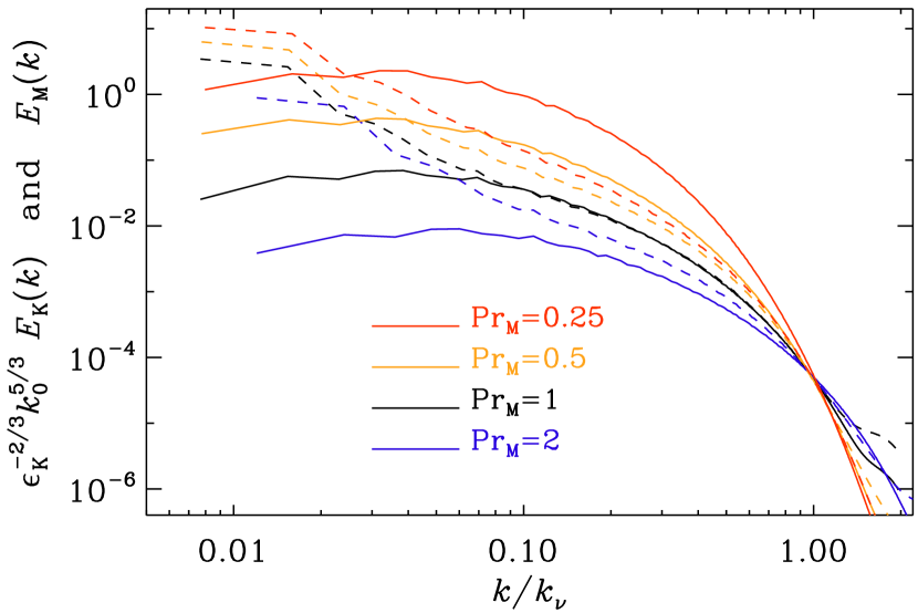
Figure 8: Magnetic energy spectra (solid lines) for nonlinearly saturated runs with $\mbox{\rm Pr}_{\rm M}=0.25$ (Run K, red), 0.5 (Run J, orange), 1 (Run I, black), and 2 (Run H, blue) along with the corresponding kinetic energy spectra (dashed lines).

We repeat a sequence of runs similar to that presented in Fig. 3, where we show that the shapes of $E_{\rm K}(k)$ and $E_{\rm M}(k)$ are similar for $\mbox{\rm Pr}_{\rm M}=\mbox{\rm Pr}_{\rm M}^{\rm crit}\approx 0.3$. In the nonlinear regime, the situation is more complicated in that now also $E_{\rm K}(k)$ changes near saturation. The nonlinear runs are denoted analogously to the kinematic case using, however, lowercase letters. They are summarized in Table 4, where all data are averaged over a statistically steady interval of length $\Delta t$. Here we also define a magnetic dissipation wavenumber analogous to Eq. (7), i.e.,

$$k_{\eta}^{\rm NL}=\left(\epsilon_{\rm M}/\rho_{0}\eta^{3}\right)^{1/4},$$ (18)

where the superscript NL should remind us that this quantity can only be defined in the nonlinear regime (because otherwise $\epsilon_{\rm M}\to 0$) and that $k_{\eta}^{\rm NL}$ is different from the $k_{\eta}$ defined by collapsing the curves $E_{\rm M}(k/k_{\eta})$ on top of each other, as in Fig. 4. In Fig. 8, we compare the shapes of $E_{\rm M}(k)$ and $E_{\rm K}(k)$ after having scaled them such that their values agree near $k=k_{\nu}$. This scaling allows us to see more readily the relative change of slopes between $E_{\rm M}(k)$ and $E_{\rm K}(k)$. We see that their profiles now agree with each other for $\mbox{\rm Pr}_{\rm M}=1$. For larger values of $\mbox{\rm Pr}_{\rm M}$, the slope of the magnetic spectrum is smaller than that of the kinetic energy spectrum, while for smaller values of $\mbox{\rm Pr}_{\rm M}$, the magnetic slopes are steeper. From this, we conclude that there is a critical value of the magnetic Prandtl number in the nonlinear regime that is of the order of unity. This result agrees with that of Kriel et al. (2022).

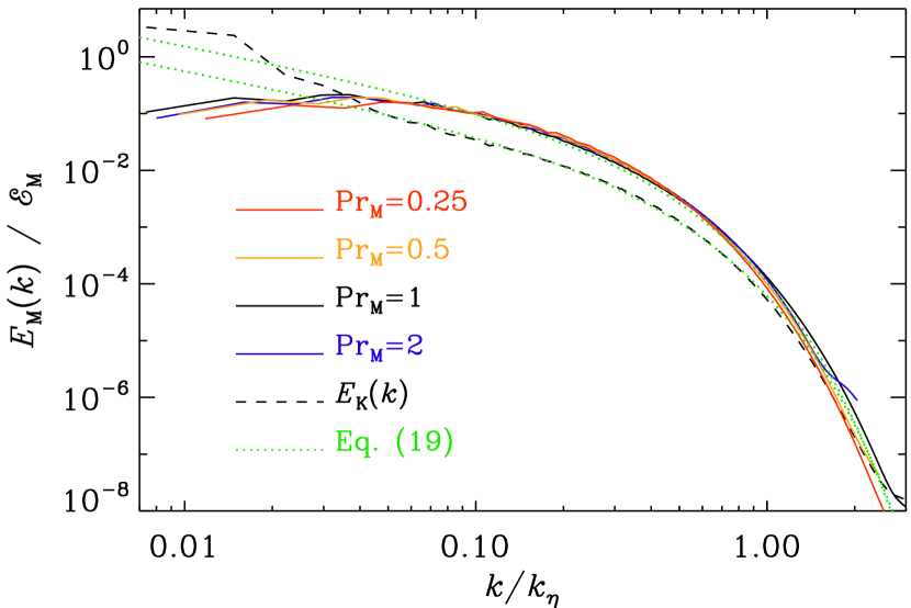
Figure 9: Similar to Fig. 4, but for the nonlinearly saturated case.

The two green lines represent the fits with Eq. (19) using the parameters in Eq. (20). In Fig. 9, we show the results of collapsing the nonlinearly saturated spectra on top of each other. Here, we use Run g with $\mbox{\rm Pr}_{\rm M}=1$ as reference run, because this value is close to the nonlinear value of $\mbox{\rm Pr}_{\rm M}^{\rm crit}$. The resulting values of $k_{\eta}$ are listed in Table 4. In this nonlinear case, Eq. (10) no longer provides a useful description of the magnetic energy spectrum. Instead, the dissipative subrange can well be described by a formula similar to Eq. (13), but with a $k^{-1}$ inertial range, i.e.,

$$E_{\rm K/M}(k)\propto k^{-1}\exp(-k/k_{\nu/\eta}^{\rm NLfit}),$$ (19)

where we find

$$k_{\nu}^{\rm NLfit}\approx 0.22\,k_{\eta},\quad k_{\eta}^{\rm NLfit}\approx 0.20\,k_{\eta}\quad\mbox{(for $\mbox{\rm Pr}_{\rm M}=1$).}$$ (20)

As in the kinematic case, $k_{\eta}$ depends on $k_{\nu}$ and $\mbox{\rm Pr}_{\rm M}$, as will be discussed next.

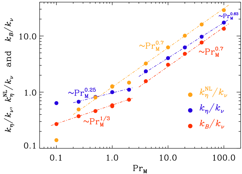
Figure 10: Similar to Fig. 2, showing the dependence of $k_{\eta}/k_{\nu}$ (closed symbols), the dependence of $k_{\eta}^{\rm NL}/k_{\nu}$ (closed symbols), and $k_{B}/k_{\nu}$ (open symbols) on $\mbox{\rm Pr}_{\rm M}$. The dashed-dotted lines show $\mbox{\rm Pr}_{\rm M}^{0.3}$ and $\mbox{\rm Pr}_{\rm M}^{0.7}$ scalings for comparison.

In Fig. 10, we plot the dependence of $k_{\eta}/k_{\nu}$, $k_{\eta}^{\rm NL}/k_{\nu}$, and $k_{B}/k_{\nu}$ on $\mbox{\rm Pr}_{\rm M}$. We see that now the slopes are different from those in the kinematic case. Specifically, we find $k_{\eta}/k_{\nu}\approx 0.95\,\mbox{\rm Pr}_{\rm M}^{0.63}$ for $\mbox{\rm Pr}_{\rm M}>3$ and $k_{\eta}/k_{\nu}\approx 0.97\,\mbox{\rm Pr}_{\rm M}^{0.25}$ for $\mbox{\rm Pr}_{\rm M}<3$. Furthermore, we find $k_{\eta}^{\rm NL}/k_{\nu}\approx 0.57\,\mbox{\rm Pr}_{\rm M}^{0.7}$ for $\mbox{\rm Pr}_{\rm M}>3$ and $k_{\eta}^{\rm NL}/k_{\nu}\approx 0.59\,\mbox{\rm Pr}_{\rm M}^{1/3}$ for $\mbox{\rm Pr}_{\rm M}<3$. The relations in Eq. (20) remain approximately valid in the neighborhood of $\mbox{\rm Pr}_{\rm M}=1$, but deteriorate significantly for $\mbox{\rm Pr}_{\rm M}\gg 1$. This is because the functional form of Eq. (19) no longer provides a good description. We refer here to earlier work (Brandenburg, 2009, 2011, 2014), where the $\mbox{\rm Pr}_{\rm M}$ dependence in the nonlinear regime has been studied in much more detail.

4 Conclusions

In this paper, we have determined the magnetic Prandtl number dependence for three rather different scales characterizing the dissipative magnetic structures in a kinematic small-scale dynamo: their diameter, their theoretical cutoff wavenumbers based on the growth rate, and the actual spectral cutoff. For a magnetic Prandtl number of about 0.3, viscous and resistive cutoff scales are found to be approximately equal. This is different from the results in the nonlinear regime, where a critical value of unity is found. A scaling of the cutoff wavenumber proportional to $\mbox{\rm Pr}_{\rm M}^{1/2}$ is found for $0.05\leq\mbox{\rm Pr}_{\rm M}\leq 100$. A change of such a scaling is expected for very small values of $\mbox{\rm Pr}_{\rm M}$, but this cannot be confirmed for moderately small values.

For the actual thickness of flux tubes, we do find a break in the scaling for $\mbox{\rm Pr}_{\rm M}\approx 1$, but it is now steeper than expected both for small and large values of $\mbox{\rm Pr}_{\rm M}$. For the scale based on the theoretically expected eigenfunction of the Kazantsev small-scale dynamo, we also found a slightly steeper scaling, but no breakpoint for smaller values of $\mbox{\rm Pr}_{\rm M}$ close to $\mbox{\rm Pr}_{\rm M}=0.05$.

For the large values of $\mbox{\rm Pr}_{\rm M}$ that are expected to occur in the interstellar medium and in galaxy clusters, the viscous scale is much larger than the resistive one and it may be observationally accessibility through an excess of the parity-even $E$ polarization over the party-odd $B$ polarization in synchrotron emission (Brandenburg et al., 2022b). The resistive scale, on the other hand, may be accessible through interstellar scintillation measurements of pulsars (Cordes et al., 1985; Rickett, 1990; Bhat et al., 2004), as discussed in the introduction. Thus, there may be ways of comparing theory with observations in the not too distant future.

It would also be interesting to extend the present study to other measures of magnetic structures. One such possibility is the use of Minkowski functionals (Sahni et al., 1998). Wilkin et al. (2007) have used this method to show that the thickness, width, and length of magnetic structures from a small-scale dynamo scale differently with magnetic Reynolds number. In their case, however, the value of Re was held constant, so $\mbox{\rm Pr}_{\rm M}$ and $\mbox{\rm Re}_{\rm M}$ did not vary independently. Furthermore, they did not actually solve the momentum equation and considered instead a prescribed flow with a given power spectrum. Subsequent work by Seta et al. (2020) demonstrated, however, that both the thickness and width of the structures show $\mbox{\rm Re}_{\rm M}^{-1/2}$ scaling. Furthermore, the structures are more space filling (Seta & Federrath, 2021).

Data Availability

The source code used for the simulations of this study, the Pencil Code (Pencil Code Collaboration et al., 2021), is freely available on http://github.com/pencil-code/. The DOI of the code is http://doi.org/10.5281/zenodo.2315093. Supplemental Material and the simulation setups with the corresponding secondary data are available on http://doi.org/10.5281/zenodo.7090887; see also http://www.nordita.org/~brandenb/projects/keta_vs_PrM for easier access to the same material as on the Zenodo site (Brandenburg et al., 2022a).

Appendix A Viscous cutoff scaling

In Sect. 2.2 we discussed the expected $\mbox{\rm Re}^{3/4}$ scaling of the viscous cutoff wavenumber. This scaling was also verified by Kriel et al. (2022), but they did not actually compute $\epsilon_{\rm K}$, nor did they use Eq. (7). To verify that $k_{\nu}$ obeys this scaling, we show in Fig. 11 the dependence of $k_{\nu}$ on Re. Quantitatively, we have $k_{\nu}/k_{\rm f}\approx 0.48\,\mbox{\rm Re}^{3/4}$. Small departures are seen for very small and very large values of Re. The latter could be related to insufficient resolution for such a high value of Re, while the former could indicate that the 3/4 scaling is not yet applicable.

Figure 11: Dependence of $k_{\nu}$ on Re with $k_{\nu}/k_{\rm f}\approx 0.48\,\mbox{\rm Re}^{3/4}$. For $\mbox{\rm Re}\approx 10$, there is no longer a proper turbulent cascade and the $3/4$ scaling is expected to become invalid. We have therefore excluded this point from the fit and have only drawn this point so that one can see that the departure is not very large yet. The error bars can hardly be noticed.

Our coefficient in the relation between $k_{\nu}/k_{\rm f}$ is larger than that found by Kriel et al. (2022). They found $k_{\nu}/k_{\rm f}\approx 0.025\,\mbox{\rm Re}_{\rm KBSF}^{3/4}$, where $\mbox{\rm Re}_{\rm KBSF}=2\pi\mbox{\rm Re}$. Thus, their relation corresponds to $k_{\nu}/k_{\rm f}\approx 0.10\,\mbox{\rm Re}^{3/4}$. However, if their effective $k_{\rm f}$ was also $1.5\,k_{1}$, as in our case, then the prefactor would be 0.07 instead of 0.1.

Appendix B Viscous cutoff wavenumber

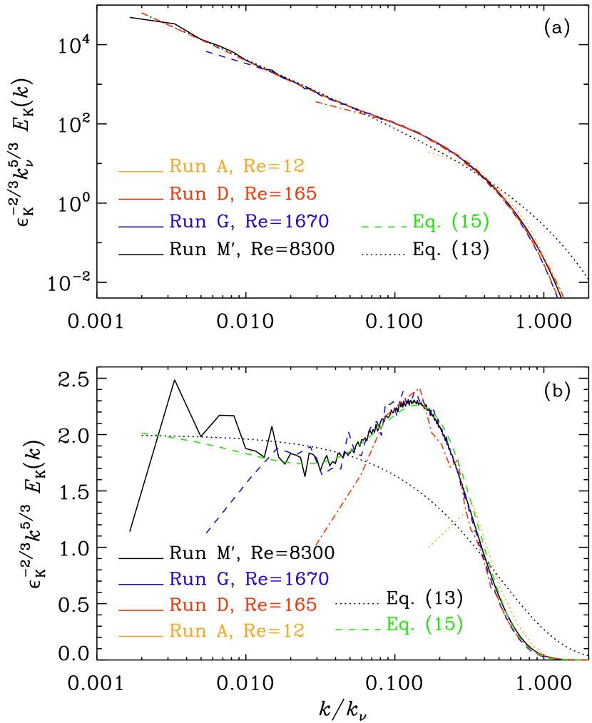
Figure 12: Kinetic energy spectra for Runs A, D, G, and M’. together with the fits given by Eqs. (13) and (15). Panel (b) shows the compensated version of the spectrum shown in panel (a). No adjustable parameters are used, except for the fits with Eqs. (13) and (15).

In Sect. 3.5, we discussed different variants of $k_{\nu}$. In Fig. 12(a), we plot kinetic energy spectra for Runs A, D, G, and M’, together with the fit given by Eq. (13) with $k_{\nu}^{\rm fit}\approx 0.5\,k_{\nu}$ and Eq. (15) with $n_{\rm bot}=1.8$, $n_{\rm dis}=0.86$, $k_{\nu}^{\rm bot}\approx 0.056\,k_{\nu}$, and $k_{\nu}^{\rm dis}\approx 0.073\,k_{\nu}$. The latter corresponds to another definition of the viscous cutoff wavenumber as $k_{\nu}^{\rm dis}$. To demonstrate more clearly the existence of the bottleneck effect in our simulations, we show in Fig. 12(b) compensated kinetic energy spectra, $\epsilon_{\rm K}^{-2/3}k^{5/3}E_{\rm K}(k)$, and compare with the fit given by Eq. (15).

References

- Armstrong et al. (1995) Armstrong J. W., Rickett B. J., Spangler S. R., 1995, ApJ, 443, 209
- Arponen & Horvai (2007) Arponen H., Horvai P., 2007, J. Stat. Phys., 129, 205
- Bannister et al. (2016) Bannister K. W., Stevens J., Tuntsov A. V., Walker M. A., Johnston S., Reynolds C., Bignall H., 2016, Science, 351, 354
- Bhat et al. (2004) Bhat N. D. R., Cordes J. M., Camilo F., Nice D. J., Lorimer D. R., 2004, ApJ, 605, 759
- Boldyrev & Cattaneo (2004) Boldyrev S., Cattaneo F., 2004, Phys. Rev. Lett., 92, 144501
- Brandenburg (2009) Brandenburg A., 2009, ApJ, 697, 1206
- Brandenburg (2011) Brandenburg A., 2011, ApJ, 741, 92
- Brandenburg (2014) Brandenburg A., 2014, ApJ, 791, 12
- Brandenburg et al. (1995) Brandenburg A., Procaccia I., Segel D., 1995, Phys. Plasmas, 2, 1148 (BPS)
- Brandenburg et al. (1996) Brandenburg A., Jennings R. L., Nordlund Å., Rieutord M., Stein R. F., Tuominen I., 1996, J. Fluid Mech., 306, 325
- Brandenburg et al. (2018) Brandenburg A., Haugen N. E. L., Li X.-Y., Subramanian K., 2018, MNRAS, 479, 2827
- Brandenburg et al. (2022a) Brandenburg A., Rogachevskii I., Schober J., 2022a, Zenodo, DOI:10.5281/zenodo.7090887
- Brandenburg et al. (2022b) Brandenburg A., Zhou H., Sharma R., 2022b, MNRAS, in press, DOI:10.1093/mnras/stac3217, p. arXiv:2207.09414
- Cho & Ryu (2009) Cho J., Ryu D., 2009, ApJL, 705, L90
- Clegg et al. (1998) Clegg A. W., Fey A. L., Lazio T. J. W., 1998, ApJ, 496, 253
- Cordes et al. (1985) Cordes J. M., Weisberg J. M., Boriakoff V., 1985, ApJ, 288, 221
- Dobler et al. (2003) Dobler W., Haugen N. E., Yousef T. A., Brandenburg A., 2003, PhRvE, 68, 026304
- Haugen et al. (2003) Haugen N. E. L., Brandenburg A., Dobler W., 2003, ApJL, 597, L141
- Haugen et al. (2004) Haugen N. E., Brandenburg A., Dobler W., 2004, PhRvE, 70, 016308
- Haugen et al. (2022) Haugen N. E. L., Brandenburg A., Sandin C., Mattsson L., 2022, JFM, 934, A37
- Kazantsev (1968) Kazantsev A. P., 1968, Sov. J. Exp. Theor. Phys., 26, 1031
- Kleeorin & Rogachevskii (2012) Kleeorin N., Rogachevskii I., 2012, Phys. Scripta, 86, 018404
- Kriel et al. (2022) Kriel N., Beattie J. R., Seta A., Federrath C., 2022, MNRAS, 513, 2457
- Kulsrud & Anderson (1992) Kulsrud R. M., Anderson S. W., 1992, ApJ, 396, 606 (KA)
- Martins Afonso et al. (2019) Martins Afonso M., Mitra D., Vincenzi D., 2019, Proc. Roy. Soc. Lond. Ser. A, 475, 20180591
- Moffatt et al. (1994) Moffatt H. K., Kida S., Ohkitani K., 1994, J. Fluid Mech., 259, 241
- Nordlund et al. (1992) Nordlund A., Brandenburg A., Jennings R. L., Rieutord M., Ruokolainen J., Stein R. F., Tuominen I., 1992, ApJ, 392, 647
- Pen & King (2012) Pen U.-L., King L., 2012, MNRAS, 421, L132
- Pencil Code Collaboration et al. (2021) Pencil Code Collaboration et al., 2021, JOSS, 6, 2807
- Politano & Pouquet (1998) Politano H., Pouquet A., 1998, Geophys. Res. Lett., 25, 273
- Qian (1984) Qian J., 1984, Phys. Fluids, 27, 2229
- Rickett (1990) Rickett B. J., 1990, ARA&A, 28, 561
- Rogachevskii & Kleeorin (1997) Rogachevskii I., Kleeorin N., 1997, PhRvE, 56, 417
- Sahni et al. (1998) Sahni V., Sathyaprakash B. S., Shandarin S. F., 1998, ApJL, 495, L5
- Scalo & Elmegreen (2004) Scalo J., Elmegreen B. G., 2004, ARA&A, 42, 275
- Schekochihin et al. (2004) Schekochihin A. A., Cowley S. C., Taylor S. F., Maron J. L., McWilliams J. C., 2004, ApJ, 612, 276
- Schober et al. (2012) Schober J., Schleicher D., Federrath C., Klessen R., Banerjee R., 2012, PhRvE, 85, 026303
- Seta & Federrath (2021) Seta A., Federrath C., 2021, PhRvF, 6, 103701
- Seta et al. (2020) Seta A., Bushby P. J., Shukurov A., Wood T. S., 2020, PhRvF, 5, 043702
- She & Jackson (1993) She Z.-S., Jackson E., 1993, Phys. Fluids A, 5, 1526
- She et al. (1990) She Z.-S., Jackson E., Orszag S. A., 1990, Natur, 344, 226
- Subramanian & Brandenburg (2014) Subramanian K., Brandenburg A., 2014, MNRAS, 445, 2930
- Tennekes & Lumley (1972) Tennekes H., Lumley J. L., 1972, First Course in Turbulence. MIT Press, Cambridge
- Vincent & Meneguzzi (1991) Vincent A., Meneguzzi M., 1991, J. Fluid Mech., 225, 1
- Warnecke et al. (2022) Warnecke J., Käpylä M., Gent F., Rheinhardt M., 2022, Nat. Astron., DOI:10.21203/rs.3.rs-1819381/v1
- Wilkin et al. (2007) Wilkin S. L., Barenghi C. F., Shukurov A., 2007, PhRvL, 99, 134501
- Xu & Zhang (2017) Xu S., Zhang B., 2017, ApJ, 835, 2
- Zeldovich et al. (1990) Zeldovich Y. B., Ruzmaikin A. A., Sokoloff D. D., 1990, The Almighty Chance. Singapore: World Scientific