Magnetically confined wind shock

Abstract

Many stars across all classes possess strong enough magnetic fields to influence dynamical flow of material off the stellar surface. For the case of massive stars (O and B types), about 10% of them harbour strong, globally ordered (mostly dipolar) magnetic fields. The trapping and channeling of their stellar winds in closed magnetic loops leads to magnetically confined wind shocks (MCWS), with pre-shock flow speeds that are some fraction of the wind terminal speed that can be a few thousand km s^-1. These shocks generate hot plasma, a source of X-rays. In the last decade, several developments took place, notably the determination of the hot plasma properties for a large sample of objects using XMM-Newton and Chandra, as well as fully self-consistent MHD modelling and the identification of shock retreat effects in weak winds. In addition, these objects are often sources of H$\alpha$ emission which is controlled by either sufficiently high mass loss rate or centrifugal breakout. Here we review the theoretical aspects of such magnetic massive star wind dynamics.

1 Keywords

Massive stars; magnetic field; rotation; x-rays; stellar winds, radiative cooling.

2 Introduction

Hot luminous, massive stars of spectral type O and B are prominent sources of X-rays which can originate from three distinct sources: shocks in their high-speed radiatively driven stellar winds, wind-wind collisions in binary systems and magnetically confined wind shocks.

In single, non-magnetic O stars, the intrinsic instability of wind driving by line-scattering leads to embedded wind shocks that are thought to be the source of their relatively soft ($\sim$0.5 keV) X-ray spectrum, with a total X-ray luminosity that scales with stellar bolometric luminosity, $L_{\rm x}\sim 10^{-7}\times L_{\rm bol}$ Chlebowski89 ; Berghoefer97 ; Naze11 . In massive binary systems the collision of the two stellar winds at up to the wind terminal speeds can lead to even higher $L_{\rm x}$, generally with a significantly harder (up to 10 keV) spectrum.

Here we discuss a third source of X-rays from OB winds, namely those observed from the subset ($\sim$10%) of massive stars with strong, globally ordered (often significantly dipolar) magnetic fields Petit13 ; in this case, the trapping and channeling of the stellar wind in closed magnetic loops leads to magnetically confined wind shocks (MCWS) BabMon1997a ; BabMon1997b , with pre-shock flow speeds that are some fraction of the wind terminal speed, resulting in intermediate energies for the shocks and associated X-rays ($\sim$2 keV). A prototypical example is provided by the magnetic O-type star $\theta^{1}$ Ori C, which shows moderately hard X-ray emission with a rotational phase variation that matches well the expectations of the MCWS paradigm Gag2005 .

Here, we focus on theoretical aspects of magnetic confinement that determine the extent of the influence of the field over the wind while the observational aspects are addressed in another chapter titled ‘X-ray emission of massive stars and their winds’. We, then, describe an effect called ‘shock retreat’, which can moderate the strength of the X-rays, or even quench it altogether in extremely low mass loss rate stars. We also review the properties and observational signatures (e.g. Balmer line emission) of the resulting magnetospheres in closed loop regions, and on the stellar rotation spindown that results from the angular momentum loss associated with magnetically torqued wind outflow from open field regions. In this way magnetic fields can have a profound effect on the star s rotational evolution, giving rotation periods ranging from weeks to even decades, in strong contrast to the day-timescale periods of non-magnetic massive stars.

3 Historical Perspective

To explain X-ray emission from the Ap/Bp star IQ Aur BabMon1997a introduced the MCWS model. In their approach, they effectively prescribed a fixed magnetic field geometry to channel the wind outflow (see also ShoBro1990 ). For large magnetic loops, wind material from opposite footpoints is accelerated to a substantial fraction of the wind terminal speed (i.e., $\geq$1000 km s^-1) before the channeling toward the magnetic field loop tops forces a collision with very strong shocks, thereby heating the gas to temperatures (10⁷ - 10⁸ K) that are high enough to emit hard (few keV) X-rays. This star has a quite strong field ($\sim$4 kG) and a rather weak wind, with an estimated mass loss rate of about $\sim 10^{-10}M_{\odot}$ yr^-1, and thus indeed could be reasonably modeled within the framework of prescribed magnetic field geometry. However, the actual X-ray emission from the star, which is predominantly soft, is further influenced by an effect called ‘shock retreat’ that we describe below. Later, BabMon1997b applied this model to explain the periodic variation of X-ray emission of the O7 star $\theta^{1}$ Ori C, which has a lower magnetic field ($\sim$1100 G) and significantly stronger wind (mass-loss rate $\sim 10^{-7}M_{\odot}$ yr^-1), raising now the possibility that the wind itself could influence the field geometry in a way that is not considered in the simple fixed-field approach.

3.1 Magnetic Confinement

In an interplay between magnetic field and stellar wind, the dominance of the field is determined by how strong it is relative to the wind. To understand the competition between these two, udDOwo2002 defined a characteristic parameter for the relative effectiveness of the magnetic fields in confining and/or channeling the wind outflow. Specifically, consider the ratio between the energy densities of field vs. flow,

$$\eta(r,\theta) \equiv \frac{B^{2}/8\pi}{\rho v^{2}/2}\approx\frac{B^{2}r^{2}}{\dot{M}v(r)}$$

$$= \left[\frac{B_{\ast}^{2}(\theta){R_{\ast}}^{2}}{\dot{M}v_{\infty}}\right]\left[\frac{(r/R_{\ast})^{-2n}}{1-R_{\ast}/r}\right]\,,$$

where the latitudinal variation of the surface field has the dipole form given by $B_{\ast}^{2}(\theta)=B_{o}^{2}(\cos^{2}\theta+\sin^{2}\theta/4)$. In general, a magnetically channeled outflow will have a complex flow geometry, but for convenience, the second equality in eqn. (3.1) simply characterizes the wind strength in terms of a spherically symmetric mass loss rate $\dot{M}=4\pi r^{2}\rho v$. The third equality likewise characterizes the radial variation of outflow velocity in terms of the phenomenological velocity law $v(r)=v_{\infty}(1-R_{\ast}/r)^{\beta}$, with $v_{\infty}$ the wind terminal speed and assumed $\beta=1$ which seems to well approximate the numerical solution of massive star winds. This equation furthermore models the magnetic field strength decline as a power-law in radius, $B(r)=B_{\ast}(R_{\ast}/r)^{(n+1)}$, where, e.g., for a dipole $n=2$.

With the spatial variations of this energy ratio thus isolated within the right square bracket, we see that the left square bracket represents a dimensionless constant that characterizes the overall relative strength of field vs. wind. Evaluating this in the region of the magnetic equator ($\theta=90^{o}$), where the tendency toward a radial wind outflow is in most direct competition with the tendency for a horizontal orientation of the field, one can thus define an equatorial ‘wind magnetic confinement parameter’,

$$\eta_{\ast} \equiv \frac{B_{\ast}^{2}(90^{\circ}){R_{\ast}}^{2}}{\dot{M}v_{\infty}}=0.4\,\frac{B_{100}^{2}\,R_{12}^{2}}{\dot{M}_{-6}\,v_{8}}.$$ (2)

where $\dot{M}_{-6}\equiv\dot{M}/(10^{-6}\,M_{\odot}$/yr), $B_{100}\equiv B_{o}/(100$ G), $R_{12}\equiv R_{\ast}/(10^{12}$ cm), and $v_{8}\equiv v_{\infty}/(10^{8}$ cm/s). In order to have any confinement, $\eta_{\ast}\geq 1$. As these stellar and wind parameters are scaled to typical values for an OB supergiant, e.g. $\zeta$ Pup, the last equality in eqn. (2) immediately suggests that for such winds, significant magnetic confinement or channeling should require fields of order few hundred G. By contrast, in the case of the Sun, the much weaker mass loss (${\dot{M}}_{\odot}\sim 10^{-14}~{}M_{\odot}$/yr) means that even a much weaker global field ($B_{o}\sim 1$ G) is sufficient to yield $\eta_{\ast}\simeq 40$, implying a substantial magnetic confinement of the solar coronal expansion. But in Bp stars the magnetic field strength can be of order kG with ${\dot{M}}_{\odot}\sim 10^{-10}~{}M_{\odot}$/yr leading $\eta_{\ast}\leq 10^{6}$. Thus, the confinement in Bp stars is very extreme.

We emphasize that $\dot{M}$ used in the above formalism is a value obtained for a spherically symmetric non-magnetic wind as the magnetic field may significantly influence the predicted circumstellar density and velocity structure.

Alfv́en Radius

The extent of the effectiveness of magnetic confinement is set by the Alfvén radius, $R_{A}$, where flow and Alfvén velocities are equal. This will also determine the extent of the largest loops and thus the highest shock velocities affecting the hardness of X-ray emission. This radius can be derived from eqn. (3.1) where the second square bracket factor shows the overall radial variation; $n$ is the power-law exponent for radial decline of the assumed stellar field, e.g. $n=2$ for a pure dipole. For a star with a non-zero field, we have $\eta_{\ast}>0$, and so given the vanishing of the flow speed at the atmospheric wind base, this energy ratio always starts as a large number near the stellar surface, $\eta(r\rightarrow R_{\ast})\rightarrow\infty$. But from there outward it declines quite steeply, asymptotically as $r^{-4}$ for a dipole, crossing unity at the Alfvén radius defined implicitly by $\eta(R_{A})\equiv 1$ leading to :

$$1=\eta_{\ast}\left[\frac{(R_{A}/R_{\ast})^{-2n}}{1-R_{\ast}/R_{A}}\right]$$ (3)

Thus, for a canonical $\beta=1$ wind velocity law, explicit solution for $R_{\rm{A}}$ along the magnetic equator requires finding the appropriate root of

$$\left({R_{A}\over R_{\ast}}\right)^{2n}-\left({R_{A}\over R_{\ast}}\right)^{2n-1}=\eta_{\ast}\,,$$ (4)

which for integer $2n$ is just a simple polynomial, specifically a quadratic, cubic, or quartic for $n=$ 1, 1.5, or 2. Even for non-integer values of $2n$, the relevant solutions can be approximated (via numerical fitting) to within a few percent by the simple general expression,

$$\frac{R_{\rm{A}}}{R_{\ast}}\approx 1+(\eta_{\ast}+1/4)^{1/(2n)}-(1/4)^{1/(2n)}\,.$$ (5)

For weak confinement, $\eta_{\ast}\ll 1$, we find $R_{\rm{A}}\rightarrow R_{\ast}$, while for strong confinement, $\eta_{\ast}\gg 1$, we obtain $R_{\rm{A}}\rightarrow\eta_{\ast}^{1/(2n)}R_{\ast}$. In particular, for the standard dipole case with $n=2$, we expect the strong-confinement scaling $R_{\rm{A}}/R_{\ast}\approx\eta_{\ast}^{1/4}$.

Clearly $R_{\rm{A}}$ represents the radius at which the wind speed $v$ exceeds the local Alfvén speed $V_{A}$. It also characterizes the maximum radius where the magnetic field still dominates over the wind. For Ap/Bp stars where stellar fields are of order kG, $\eta_{\ast}\gg 1$, e.g. for $\sigma$ Ori E it is about $10^{7}$, implying an Alfvèn radius $\sim 60R_{\ast}$. Thus, in Bp (and Ap) stars wind is trapped to large radii creating extensive magnetospheres. This also implies that X-rays from Bp stars should be intrinsically hard. But as we show below, shock retreat effects may soften it significantly.

3.2 Rotation and Kepler Radius

Another important parameter, rotation, can have dynamical effects and can be parameterized (see Uddoula08 ) in terms of the orbital rotation fraction,

$$W\equiv\frac{V_{rot}}{V_{orb}}=\frac{V_{rot}}{\sqrt{GM_{\ast}/R_{\ast}}}\,$$ (6)

where $V_{rot}$ is the star‘s equatorial rotation speed and $V_{orb}$ is the Keplerian orbital speed near the equatorial surface radius $R_{\ast}$. Insofar as the field within the Alfvèn radius is strong enough to maintain rigid-body rotation, the Kepler corotation radius $R_{K}$ identifies where the centrifugal force for rigid-body rotation exactly balances the gravity in the equatorial plane. If $R_{A}<R_{K}$, then material trapped in closed loops will again eventually fall back to the surface, forming a dynamical magnetosphere (DM). But if $R_{A}>R_{K}$, then wind material located between $R_{K}$ and $R_{A}$ can remain in static equilibrium, forming a centrifugal magnetosphere (CM) that is supported against gravity by the magnetically enforced co-rotation. This is illustrated by figure 1. We can then compute $R_{K}$ readily from:

$$R_{K}=W^{-2/3}R_{\ast}.$$ (7)

Figure 1: Sketch of the regimes for a dynamical vs. centrifugal magnetosphere (DM vs. CM).

Figure 2: For a 2D MHD simulation of a magnetized wind with confinement parameter $\eta_{\ast}=100$, (Uddoula14 ) color plots of log density (left) and log temperature (middle) for arbitrary snapshot many dynamical times after initialization. Note that magnetic loops for initially a dipole field extending above $R_{\mathrm{A}}/R_{\ast}\approx 100^{1/4}\approx 3.2$ are drawn open by the wind, while those with an apex below $R_{\mathrm{A}}$ remain closed. The right panel plots associated X-ray emission from the magnetically confined wind shock (MCWS) near the apex of closed loops.

Figure 3: Top: Contour plot for density at an arbitrary snapshot of an isothermal 2D MHD simulation, overlayed with illustration to define the radial mass distribution, $\Delta m/\Delta r$ near the equator. Bottom: Color plots for log of $\Delta m/\Delta r$, plotted versus radius (1-5 $R_{\ast}$) and time (0-3 Msec), for a mosaic of 2-D MHD models with a wide range of magnetic confinement parameters $\eta_{\ast}$, and 3 orbital rotation fractions $W$. The horizontal solid lines indicate the Alfvén radius $R_{\rm A}$ (solid) and Kepler radius $R_{\rm K}$ (dashed).

MHD Simulations

The initial magnetohydrodynamic (MHD) simulations by udDOwo2002 assumed, for simplicity, that radiative heating and cooling would keep the wind outflow nearly isothermal at roughly the stellar effective temperature. The simulations studied the dynamical competition between field and wind by evolving MHD simulations from an initial condition when a dipole magnetic field is suddenly introduced into a previously relaxed, one-dimensional spherically symmetric wind.

Immediately after the introduction of the field, the dynamic interplay between the wind and the field leads to two distinct regions. Along the polar region, the wind freely streams radially outward, stretching the field lines into a radial configuration, as can be inferred from the left panel of illustrative Fig. 2. If the field is strong enough, around the magnetic equator a region of closed magnetic loops is formed wherein the flow from opposite hemispheres collides to make strong shocks, quite similar to what was predicted in the semi-analytic, fixed-field models of BabMon1997a . The shocked material forms a dense disk-like structure which is opaque to line-driving. But its support against gravity by the magnetic tension along the convex field lines is inherently unstable, leading to a complex pattern of fall back along the loop lines down to the star, again as suggested by the left panel of Fig. 2 .

Note that even for weak field models with moderately small confinement, $\eta_{\ast}\leq 1/10$, the field still has a noticeable global influence on the wind, enhancing the density and decreasing the flow speed near the magnetic equator. However, shock speeds are probably not large enough to produce any X-rays in that case.

The mosaic of color plots in figure 3 shows the time vs. height variation of the equatorial mass distribution $\Delta m/\Delta r$ for various combinations of rotation fraction $W$ and wind confinement $\eta_{\ast}$. Note the DM infall for material trapped below $R_{\rm K}$ and $R_{\rm A}$, vs. the dense accumulation of a CM from confined material near and above $R_{\rm K}$, but below $R_{\rm A}$.

This diagram thus provides a vivid way to characterize how the global geometry and time evolution of magnetospheres of massive stars (MSMS) depends on rotation and magnetic confinement. However, it is based entirely on the special case of field-aligned rotation in 2D.

To model the actual X-ray emission from shocks that form from the magnetic channeling and confinement, subsequent efforts udD2003 ; Gag2005 have relaxed the assumption of isothermal equation of state in earlier studies to include a detailed energy equation that follows the radiative cooling of shock-heated material. The MCWS model provides excellent agreement with the diagnostics from the phase-resolved Chandra spectroscopy of $\theta^{1}$ Ori C (Gag2005, ).

Rotation-confinement diagram and stellar spindown

This theoretical characterization of the properties of MSMS provides an instructive way to classify their observational characteristics within a rotation vs. magnetic confinement diagram. For the still-growing list of observationally confirmed magnetic hot-stars (with $T_{\mathrm{eff}}\geq 16$ kK) compiled by (Petit13, ), the left panel of figure 4 plots positions in a log-log plane of $R_{\rm K}$ vs. $R_{\rm A}$. The diagonal line representing $R_{\rm K}=R_{\rm A}$ divides the domain of CMs to the upper right from that for DMs to the lower left. Note that almost all all O-stars are located among the slow rotators in the lower left, a direct consequence of their rapid spindown from the loss of angular momentum in their strong, magnetized winds.

In DMs, all the material trapped in closed magnetic loops eventually falls back to the star, and so balances the input from the upflowing stellar wind. This can greatly reduce the overall net mass loss, implying a higher final remnant mass in the stellar evolution that could help explain the large masses inferred from LIGO gravitational wave detections of black hole mergers (Petit17, ). Within such closed loops, the overall structure of shocked-heated gas, followed by cooling and infall, is well characterized by an analytic dynamical magnetosphere (ADM; Owocki16, ) model. As discussed in this chapter, this generalized ADM model has proven quite useful for interpreting general trends in observational diagnostics like X-ray emission (Uddoula14, ), UV wind line variations (Erba19, ), and H-alpha emission (Sundqvist12, ).

2D MHD aligned-dipole simulations (Uddoula09, ) have indicated that the angular momentum carried out by a magnetically torqued stellar wind follows the same simple, split-monopole scaling law derived for the Sun by (Weber67, ), $\dot{J}=\frac{2}{3}{\dot{M}}\,\Omega\,R_{\rm A}^{2}$ – with, however, the Alfvén radius $R_{\rm A}$ now given by the dipole scaling $R_{\rm A}\sim\eta_{\ast}^{1/4}$ (see equation 5 for $\eta_{\ast}\gg 1$ and $n=2$), instead the oft-quoted, stronger scaling ($R_{\rm A}\sim\eta_{\ast}^{1/2}$) for a split monopole. This leads to an associated general formula for the rotational spindown timescale,

$$\tau_{\rm J}\equiv\frac{I\Omega}{{\dot{J}}}=\frac{3}{2}f\tau_{\rm mass}\,\left(\frac{R_{\ast}}{R_{\rm A}}\right)^{2}\approx 0.15\frac{\tau_{\rm mass}}{\sqrt{\eta_{\ast}}}\,,$$ (8)

where $\tau_{\rm mass}\equiv M/{\dot{M}}$ is the stellar mass loss timescale, and $f$ is a dimensionless measure of the star’s moment of inertia $I\equiv fMR_{\ast}^{2}$. For the case of a rigid sphere $f\equiv\frac{2}{5}$, but massive stars with convective cores and radiative envelopes rarely behave like a rigid sphere, and assumed value $f\approx 0.1$ in the above equation is a good approximation.

This can be used to define a star’s maximum spindown age $\tau_{\mathrm{J}}$ (i.e., the number of spindown e-folds from an assumed critical initial rotation) in terms of its inferred present-day critical rotation fraction $W$ relative to an assumed initial critical rotation $W_{o}=1$, $t_{\mathrm{s,max}}={\tau_{\mathrm{J}}}(\ln{W_{o}/W})$. In figure 4 the upper axis gives the spindown timescale $\tau_{\mathrm{J}}$ (normalized by the value in a non-magnetized wind), while the right axis gives the maximum spindown age $t_{\mathrm{s,max}}$ (normalized by the spindown time). Stars above the horizontal dotted line have a maximum spindown age that is less than a single spindown time. All the most rapidly rotating stars are cooler B-type with weak winds, and thus weak braking, despite their strong field. This spindown scaling thus forms the basis for modeling the rotational evolution of magnetic massive stars (Keszthelyi20, ). It explains why nearly all the magnetic O-stars are slow rotators. Moreover, application to the prototypical magnetic B-star $\sigma$ Ori E  shows good agreement with the spindown directly inferred from extended monitoring of the timing of magnetospheric clouds transiting in front of the star (Tow2010, ).

Despite this general success, a key open question regards how this angular momentum loss scaling, which is based on 2D simulations of field-aligned dipole cases, might be altered by 3D effects for tilted dipoles or higher-order multipoles. Current preliminary results from 3D MHD simulations indicate that the effects are of order unity.

Figure 4: Classification of observationally confirmed magnetic massive stars in terms of magnetic confinement vs. rotation fraction, characterized here by a log-log plot of Kepler radius $R_{\rm K}$ increasing downward vs. Alfvén radius $R_{\rm A}$ increasing to the right (Petit13, ). The diagonal line separates the domains of dynamical magnetospheres (DM) with $R_{\rm A}<R_{\rm K}$ vs. centrifugal magnetospheres (CM) with $R_{\rm A}>R_{\rm K}$. The additional upper and right axes give respectively the corresponding spindown timescale $\tau_{\mathrm{J}}$ and maximum spindown age $t_{\mathrm{s,max}}$ (see equation 8 and following text). Rapidly rotating stars above the horizontal dotted line have $t_{\mathrm{s,max}}<\tau_{\mathrm{J}}$.

Figure 5: Upper left: Schematic showing “shock retreat” that depends on the input mass flux into a closed magnetic loops. Upper right: Comparison of resulting “XADM” scaling relations (for X-rays from analytic dynamical magnetospheres) with time-averaged X-ray emission from 2D MHD simulations with $\eta_{\ast}=10$ (blue) and $\eta_{\ast}=100$ (black) (with bolder curves showing results when inverse-Compton cooling is also included). The dotted curves are for the XADM analytic scaling for the same models. Lower left: Radius and time evolution of X-rays from MCWS in these 2D MHD simulations of DMs, showing the cycle of build up and decay, leading to the 20% duty-cycle reduction compared with the XADM scalings. Lower right: Compilation (Naze14, ) of the observed X-ray luminosity of magnetic stars, compared with the prediction of the XADM model with a reduced 10% duty-cycle factor. The agreement is best for slowly rotating DM stars with open circles (O-stars) and triangles (B-stars). The stars within the magenta box, which show an order of magnitude higher X-ray emission, are almost all rapidly rotating B-stars with CMs (filled triangles).

3.3 X-ray luminosity from magnetically confined wind shocks

For the DM cases without dynamically significant rotation, i.e. small values of $W$, Uddoula14 carried out a more systematic 2D MHD simulation parameter study with a full energy equation to compute the X-ray luminosity $L_{x}$ that results from magnetically confined wind shocks. These MHD simulation results were used to calibrate an ‘X-ray Analytic Dynamical Magnetosphere’ (XADM) analysis for how the overall X-ray luminosity scales with stellar magnetic field strength and wind mass loss rate.

Figure 5 shows some key results, together with comparison with observed X-ray data. The X-ray emission is largely controlled by a shock retreat effect (upper left panel) that depends on the wind feeding rate, and the associated radiative cooling length. The upper-right panel plots the ratio $L_{x}/L_{bol}$ vs. wind feeding rate ${\dot{M}}$ for models with magnetic confinement $\eta_{\ast}=10$ (blue) and $100$ (black), compared with prediction scalings (dashed curves) from the XADM analysis. For the most luminous stars, $L_{x}$ scales in proportion to the wind mass loss rate, but at lower $L_{bol}$, the lower $\dot{M}$ means the radiative cooling becomes inefficient, leading to shock retreat such that weaker and softer X-rays are produced. The lower-left panel showing the radius and time evolution of the X-ray emission exhibits episodes of little emission associated with intervals of matter infall, without shock heating. This overall duty-cycle lowers the averaged emission frequency relative to the idealized XADM analysis.

The lower right panel of figure 5 shows that the XADM model with a 10% efficiency matches quite well the trend in observed X-rays for a large sample of DM stars, over more that four decades in X-ray flux. Stars in the magenta box, which are X-ray over-luminous relative to this XADM scaling, are in fact mostly rapid rotators with CMs. This could possibly be explained, e.g., by enhanced centrifugal acceleration that leads to stronger shocks, and thus harder, more intense X-ray emission; or, perhaps, by centrifugal (CBO) events and the associated heating by magnetic reconnection to X-ray emitting temperatures. For a more definitive answer, further future study must be undertaken.

3.4 UV wind line variation observed by HST

The magnetic channeling of a hot-star wind outflow can also impart distinct signatures on UV wind lines that can be observed with Hubble Space Telescope (HST) (David-Uraz19, ). In particular, multiple time exposures of slowly rotating magnetic O-stars show variations in the absorption troughs of UV P-Cygni lines like SiIV and CIV, with the most distinctive signatures seen in the O7f?cp star NGC 1624-2, the most strongly magnetic O-star known (David-Uraz21, ).

This and other magnetic O-stars are too slowly rotating to have CMs; but they are nonetheless inferred to have field tilts that give rotational changes in observer perspective, leading in NGC 1624-2 to variation from a ‘high state’ (with deeper, faster absorption) and a ‘low state’ (with shallower, slower absorption). Figure 6 shows how such profiles can be modeled using the ADM formalism in terms of whether the observer views along the magnetic pole or equator of a tilted dipole ((Erba17, ; Erba19, ). Similar spectral line-profile variations are seen in multiple HST exposures from other magnetic O-stars (David-Uraz19, ).

Figure 6: Top: HST spectra of Si IV (left panel) and C IV (right panel) from two non-magnetic O-star (HD 93146, top spectrum, and HD 36861, bottom spectrum) compared with separate exposures from the strongly magnetic O-star NGC1624-2, showing both a ‘high’ and ‘low’ state. Bottom: Synthetic line profiles showing how these Si IV lines (left) and C IV lines (right) can be modeled with the analytic dynamical magnetosphere (ADM) as arising from the difference between polar and equatorial views of a tilted dipole field (Erba17, ; Erba19, ).

Figure 7: Location of magnetic massive stars in a $\log$-$\log$ plot of $R_{\mathrm{A}}/R_{\mathrm{K}}$ vs. stellar luminosity. The symbol shadings mark the presence (pink or shaded) or absence (black) of magnetospheric H$\alpha$ emission. The main text discusses how centrifgual breakout (CBO) explains this onset of H$\alpha$ emission.

Figure 8: 3D MHD model of the dynamical magnetosphere for the young, slowly rotating (15.4-day period) O7V star $\theta^{1}$ Ori C(Uddoula13, ). The left panel shows a snapshot of wind structure drawn as isodensity surface, colored to show radial component of velocity. The middle panels show the predicted equatorial and polar views of H$\alpha$ line-center surface brightness, along with corresponding line-flux profiles. The right panel compares the observed rotational modulation of the H$\alpha$ equivalent width (black) with 3D model predictions (red) assuming a pure-dipole surface field tilted by $\beta=45^{\circ}$ to the rotation axis, as viewed from the inferred observer inclination of $i=45^{\circ}$.

3.5 H$\alpha$ line emission from Dynamical Magnetospheres

The figure 7 plots the observed magnetic stars in a plane comparing the ratio $R_{\rm A}/R_{\rm K}$ vs. stellar luminosity, with now the symbol coded to mark the presence (light shading) or absence (black) of magnetospheric H$\alpha$ emission. The horizontal solid line marks the transition between the CM domain above and the DM domain below, while the vertical dashed line marks the observational divide between O- and B-type main sequence stars. Note that all O-stars show H$\alpha$ emission, even though they are located among the slow rotators with a DM. By contrast, most B-type stars only show H$\alpha$ emission if they are well above the $R_{\rm A}/R_{\rm K}=1$ horizontal line, implying a relatively fast rotation and strong confinement that leads to a CM.

The basic explanation for this dichotomy is straightforward. The stronger winds driven by the higher luminosity O-stars can accumulate even within a relatively short dynamical timescale to a sufficient density to give the strong H$\alpha$ emission in a DM, while the weaker winds of lower luminosity B-stars require the longer confinement and buildup of a CM to reach densities required for such emission. This general picture is confirmed by the detailed dynamical models of DM and CM H$\alpha$ emission that motivated this empirical classification udD2009 ; Sundqvist12 .

For the slowly rotating O-stars HD 191612 and $\theta^{1}$ Ori C  the relative unimportance of centrifugal effects allows both 2D and 3D MHD simulations (Sundqvist12, ; Uddoula13, ) of the wind-fed DM, reproducing quite well the rotational variation of H$\alpha$ emission. For the 3D simulations of $\theta^{1}$ Ori C, figure 8 shows how wind material trapped in closed loops over the magnetic equator (left panel) leads to circumstellar emission that is strongest during rotational phases corresponding to pole-on views (middle panel). For a pure dipole with the inferred magnetic tilt $\beta=45^{\circ}$, an observer with the inferred inclination $i=45^{\circ}$ has perspectives that vary from magnetic pole to equator, leading in the 3D model to the rotational phase variations in H$\alpha$ equivalent width shown in the right panel (red squares). This matches quite well both the modulation and random fluctuation of the observed equivalent width (black dots).

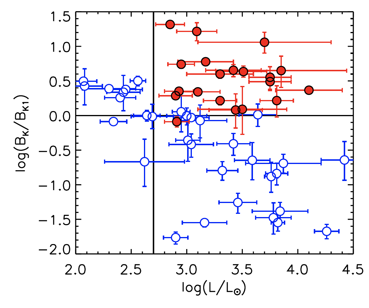
Figure 9: Top: Schematic to show the process of centrifugal breakout (CBO). Center: For the magnetic B-star sample from Shultz21 , measured equivalent width (EW) of H$\alpha$ emission vs. predicted values from the CBO model. Bottom: The same sample as above plotted as $\log B_{K}/B_{K1}$ vs. $\log L/L_{\odot}$, with stars showing H$\alpha$ emission in filled red circles, and those without in open blue circles. Here $B_{K}$ is the observationally inferred field strength at the Kepler co-rotation radius $R_{\mathrm{K}}$, while $B_{K1}$ is the strength the CBO predicts is needed to make the CM have unit optical thickness in H$\alpha$ at $R_{\mathrm{K}}$. Note the remarkable agreement of the CBO predictions for both the onset and level of H$\alpha$ emission. (Low luminosity stars to the left of the vertical line may have too weak a wind to fill the CM over other competing leakage mechanisms.)

3.6 Centrifugal Breakout and H$\alpha$ emission from Centrifugal Magnetospheres

In contrast to the dynamical cycle of upflow and infall in DMs, for CMs it is less clear how the mass buildup from the trapping of material between $R_{\rm K}$ and $R_{\rm A}$ is to be balanced. One possibility is that outward drift and diffusion from turbulent cross-field transport allows a gradual, quasi-steady leakage that balances the wind-feeding after a certain level of buildup, which depends on the mass filling rate and the magnitude of the turbulent transport coefficients (Owocki18, ).

But recent studies of H$\alpha$ emission from CMs (Shultz20, ; Owocki20, ) seem to strongly favor a CBO paradigm, in which magnetic confinement of mass in the co-rotating CM builds up until the centrifugal force overwhelms the magnetic tension, leading then to sporadic episodes of CBO, e.g., as seen in the $\Delta m/\Delta r$ plots of figure 3.

Figure 9 shows that this CBO model explains well both the onset and equivalent width of H$\alpha$ emission. In the bottom panel, $B_{K1}$ represents a prediction of the CBO analysis for the magnetic field strength at the Kepler radius needed to make the CM have unit optical depth in H$\alpha$ there; note that only B-stars with $B_{K}>B_{K1}$ exhibit emission, showing its onset occurs just at the field strength needed to confine material to the density to make the CM optically thick in H$\alpha$. The center panel shows further a very good agreement between the observed vs. CBO-predicted equivalent width of H$\alpha$.

Moreover, Shultz21 indicate that detections of non-thermal radio emission from the magnetic B-stars lie in a very similar region of the rotation-confinement diagram as H$\alpha$, implying that it too depends on a combination of strong confinement and rapid rotation. Models currently being developed indicate this too may be explained by CBO, through acceleration of electrons in CBO-driven magnetic reconnection, followed by their gyro-emission in the magnetic field.

3.7 CBO challenges to rigid-field models

Figure 10: For for a tilted dipole case with W=1/2 and $\beta=45^{\circ}$, a direct comparison of the RRM model and a preliminary 3D MHD simulation, done with a 3D implementation of the Pluto MHD code, here for a case with large magnetic confinement, $\eta_{\ast}=1000$. The plot shows column density viewed from inclination $i=90^{\circ}$ at 3 representative rotational phases. Note the significant differences in both azimuthal and latitudinal distribution of mass, which will lead to essential differences in observational signatures.

These recent results favoring CBO present a challenge to previous attempts to use an idealization of a purely rigid-field to model CMs. The Rigidly Rotating Magnetosphere (RRM; Tow2005, ) model provides a semi-analytical prescription for the 3D magnetospheric plasma distribution, based on the form and minima of the total gravitational-plus-centrifugal potential along each separate field line. The Rigid-Field Hydrodynamics (RFHD; Tow2008, ) approach carries out separate hydrodynamical simulations of wind flow on a large number ($>1000$) of rigid field lines, to derive both the shocked feeding and final settlement of material at such potential minima. Both approaches have provided an instructive basis for 3D models of CM’s with tilted dipoles or even complex fields, along with associated observational diagnostics like H$\alpha$ and X-ray emission (Tow2008, ; Oksala2012, ).

However, because they provide no mechanisms for emptying the mass build-up from wind material trapped in the CM above the Kepler radius, the resulting mass distribution is simply set by the local wind feeding rate, with a value that increases secularly with an arbitrarily assumed ‘filling time’.

Moreover, while the rigid-field assumption seems well justified in guiding the wind outflow – for which the associated confinement parameters can be as high as $\eta_{\ast}=10^{6}$ –, the notion that CBO controls the ultimate mass escape that balances the wind feeding implies that the field in such CMs must be under active dynamic stress, and so no longer acting as a purely rigid guide. The net effects of such CBO distortions on the overall 3D plasma distribution are thus not yet understood and further investigations are necessary.

Figure 10 shows some preliminary results comparing 3D MHD simulations (using a 3D version of Pluto) with the RRM model. Understanding the reasons for the clear differences will be a central focus of a future study.

4 Future Outlook

Magnetic massive stars are sources of hard X-ray emission. To understand fully how MCWS paradigm works in real stars, we need improved 3D MHD modelling that includes full energy equation with an appropriate radiative cooling. Most current 3D MHD models use isothermal equation of state whereas the RRM model lacks the necessary wind dynamics. In addition, we need to have a better understanding what role rotation plays in magnetic massive stars. The CBO paradigm provides us with a clear clue, but it does not provide us with a detailed mechanism how such continuous small scale breakout events take place.

5 Cross-References

For the observational aspects of MCWS, please see the chapter by Gregor Rauw.

References

- (1) T. Chlebowski, F. R. Harnden, Jr., and S. Sciortino, “The Einstein X-ray Observatory Catalog of O-type stars,” ApJ, vol. 341, pp. 427–455, June 1989.
- (2) T. W. Berghoefer, J. H. M. M. Schmitt, R. Danner, and J. P. Cassinelli, “X-ray properties of bright OB-type stars detected in the ROSAT all-sky survey.,” A&A, vol. 322, pp. 167–174, June 1997.
- (3) Y. Nazé, P. S. Broos, L. Oskinova, L. K. Townsley, D. Cohen, M. F. Corcoran, N. R. Evans, M. Gagné, A. F. J. Moffat, J. M. Pittard, G. Rauw, A. ud-Doula, and N. R. Walborn, “Global X-ray Properties of the O and B Stars in Carina,” ApJS, vol. 194, p. 7, May 2011.
- (4) V. Petit, S. P. Owocki, G. A. Wade, D. H. Cohen, J. O. Sundqvist, M. Gagné, J. Maíz Apellániz, M. E. Oksala, D. A. Bohlender, T. Rivinius, H. F. Henrichs, E. Alecian, R. H. D. Townsend, A. ud-Doula, and MiMeS Collaboration, “A magnetic confinement versus rotation classification of massive-star magnetospheres,” MNRAS, vol. 429, pp. 398–422, Feb. 2013.
- (5) J. Babel and T. Montmerle, “X-ray emission from Ap-Bp stars: a magnetically confined wind-shock model for IQ Aur.,” A&A, vol. 323, pp. 121–138, July 1997.
- (6) J. Babel and T. Montmerle, “On the Periodic X-Ray Emission from the O7 V Star theta 1 Orionis C,” ApJ, vol. 485, p. L29, Aug. 1997.
- (7) M. Gagné, M. E. Oksala, D. H. Cohen, S. K. Tonnesen, A. ud-Doula, S. P. Owocki, R. H. D. Townsend, and J. J. MacFarlane, “Chandra HETGS Multiphase Spectroscopy of the Young Magnetic O Star Orionis C,” ApJ, vol. 628, pp. 986–1005, Aug. 2005.
- (8) S. N. Shore and D. N. Brown, “Magnetically controlled circumstellar matter in the helium-strong stars,” ApJ, vol. 365, pp. 665–676, Dec. 1990.
- (9) A. ud-Doula and S. P. Owocki, “Dynamical Simulations of Magnetically Channeled Line-driven Stellar Winds. I. Isothermal, Nonrotating, Radially Driven Flow,” ApJ, vol. 576, pp. 413–428, Sept. 2002.
- (10) A. ud-Doula, S. P. Owocki, and R. H. D. Townsend, “Dynamical simulations of magnetically channelled line-driven stellar winds - II. The effects of field-aligned rotation,” MNRAS, vol. 385, pp. 97–108, Mar. 2008.
- (11) A. ud-Doula, S. Owocki, R. Townsend, V. Petit, and D. Cohen, “X-rays from magnetically confined wind shocks: effect of cooling-regulated shock retreat,” MNRAS, vol. 441, pp. 3600–3614, July 2014.
- (12) A. ud-Doula, The effects of magnetic fields and field-aligned rotation on line-driven hot-star winds. PhD thesis, University of Delaware, Feb. 2003.
- (13) V. Petit, Z. Keszthelyi, R. MacInnis, D. H. Cohen, R. H. D. Townsend, G. A. Wade, S. L. Thomas, S. P. Owocki, J. Puls, and A. ud-Doula, “Magnetic massive stars as progenitors of ‘heavy’ stellar-mass black holes,” MNRAS, vol. 466, pp. 1052–1060, Apr. 2017.
- (14) S. P. Owocki, A. ud-Doula, J. O. Sundqvist, V. Petit, D. H. Cohen, and R. H. D. Townsend, “An ‘analytic dynamical magnetosphere’ formalism for X-ray and optical emission from slowly rotating magnetic massive stars,” MNRAS, vol. 462, pp. 3830–3844, Nov. 2016.
- (15) C. Erba, A. David-Uraz, and V. Petit, “Quantitative Modeling of the Ultraviolet Spectra of Magnetic Massive Stars.” HST Proposal, June 2019.
- (16) J. O. Sundqvist and S. P. Owocki, “Clumping in the inner winds of hot, massive stars from hydrodynamical line-driven instability simulations,” MNRAS, p. 144, Nov. 2012.
- (17) A. ud-Doula, S. P. Owocki, and R. H. D. Townsend, “Dynamical simulations of magnetically channelled line-driven stellar winds - III. Angular momentum loss and rotational spin-down,” MNRAS, vol. 392, pp. 1022–1033, Jan. 2009.
- (18) E. J. Weber and J. Davis, Leverett, “The Angular Momentum of the Solar Wind,” ApJ, vol. 148, pp. 217–227, Apr. 1967.
- (19) Z. Keszthelyi, G. Meynet, M. E. Shultz, A. David-Uraz, A. ud-Doula, R. H. D. Townsend, G. A. Wade, C. Georgy, V. Petit, and S. P. Owocki, “The effects of surface fossil magnetic fields on massive star evolution - II. Implementation of magnetic braking in MESA and implications for the evolution of surface rotation in OB stars,” MNRAS, vol. 493, pp. 518–535, Jan. 2020.
- (20) R. H. D. Townsend, M. E. Oksala, D. H. Cohen, S. P. Owocki, and A. ud-Doula, “Discovery of Rotational Braking in the Magnetic Helium-strong Star Sigma Orionis E,” ApJ, vol. 714, pp. L318–L322, May 2010.
- (21) Y. Nazé, V. Petit, M. Rinbrand, D. Cohen, S. Owocki, A. ud-Doula, and G. A. Wade, “X-Ray Emission from Magnetic Massive Stars,” ApJS, vol. 215, p. 10, Nov. 2014.
- (22) A. David-Uraz, C. Erba, V. Petit, A. W. Fullerton, F. Martins, N. R. Walborn, R. MacInnis, R. H. Barbá, D. H. Cohen, J. Maíz Apellániz, Y. Nazé, S. P. Owocki, J. O. Sundqvist, A. ud-Doula, and G. A. Wade, “Extreme resonance line profile variations in the ultraviolet spectra of NGC 1624-2: probing the giant magnetosphere of the most strongly magnetized known O-type star,” MNRAS, vol. 483, pp. 2814–2824, Feb. 2019.
- (23) A. David-Uraz, V. Petit, M. E. Shultz, A. W. Fullerton, C. Erba, Z. Keszthelyi, S. Seadrow, and G. A. Wade, “New observations of NGC 1624-2 reveal a complex magnetospheric structure and underlying surface magnetic geometry,” MNRAS, vol. 501, pp. 2677–2687, Feb. 2021.
- (24) C. Erba, A. David-Uraz, V. Petit, and S. P. Owocki, “New Insights into the Puzzling P-Cygni Profiles of Magnetic Massive Stars,” in The Lives and Death-Throes of Massive Stars (J. J. Eldridge, J. C. Bray, L. A. S. McClelland, and L. Xiao, eds.), vol. 329, pp. 246–249, Nov. 2017.
- (25) A. ud-Doula, J. O. Sundqvist, S. P. Owocki, V. Petit, and R. H. D. Townsend
- (26) A. ud-Doula, S. P. Owocki, and R. H. D. Townsend, “Dynamical simulations of magnetically channelled line-driven stellar winds - III. Angular momentum loss and rotational spin-down,” MNRAS, vol. 392, pp. 1022–1033, Jan. 2009.
- (27) S. P. Owocki and S. R. Cranmer, “Diffusion-plus-drift models for the mass leakage from centrifugal magnetospheres of magnetic hot-stars,” MNRAS, vol. 474, pp. 3090–3100, Mar. 2018.
- (28) M. E. Shultz, S. Owocki, T. Rivinius, G. A. Wade, C. Neiner, E. Alecian, O. Kochukhov, D. Bohlender, A. ud-Doula, J. D. Landstreet, J. Sikora, A. David-Uraz, V. Petit, P. Cerrahoğlu, R. Fine, G. Henson, MiMeS Collaboration, and BinaMIcS Collaboration, “The magnetic early B-type stars - IV. Breakout or leakage? H emission as a diagnostic of plasma transport in centrifugal magnetospheres,” MNRAS, vol. 499, pp. 5379–5395, Dec. 2020.
- (29) S. P. Owocki, M. E. Shultz, A. ud-Doula, J. O. Sundqvist, R. H. D. Townsend, and S. R. Cranmer, “How the breakout-limited mass in B-star centrifugal magnetospheres controls their circumstellar H emission,” MNRAS, vol. 499, pp. 5366–5378, Dec. 2020.
- (30) M. E. Shultz, S. Owocki, T. Rivinius, G. A. Wade, C. Neiner, E. Alecian, O. Kochukhov, D. Bohlender, A. ud-Doula, J. D. Landstreet, J. Sikora, A. David-Uraz, V. Petit, P. Cerrahoğlu, R. Fine, G. Henson, G. Henson, MiMeS Collaboratio, and BinaMIcS Collaboration, “The magnetic early B-type stars - IV. Breakout or leakage? H emission as a diagnostic of plasma transport in centrifugal magnetospheres,” MNRAS, vol. 499, pp. 5379–5395, Dec. 2020.
- (31) R. H. D. Townsend, S. P. Owocki, and D. Groote, “The Rigidly Rotating Magnetosphere of Orionis E,” ApJ, vol. 630, pp. L81–L84, Sept. 2005.
- (32) R. H. D. Townsend, “Exploring the photometric signatures of magnetospheres around helium-strong stars,” MNRAS, vol. 389, pp. 559–566, Sept. 2008.
- (33) M. E. Oksala, G. A. Wade, R. H. D. Townsend, S. P. Owocki, O. Kochukhov, C. Neiner, E. Alecian, and J. Grunhut, “Revisiting the Rigidly Rotating Magnetosphere model for Ori E - I. Observations and data analysis,” MNRAS, vol. 419, pp. 959–970, Jan. 2012.