Revisiting Rolling Shutter Bundle Adjustment:
Toward Accurate and Fast Solution

Abstract

We propose an accurate and fast bundle adjustment (BA) solution that estimates the 6-DoF pose with an independent RS model of the camera and the geometry of the environment based on measurements from a rolling shutter (RS) camera. This tackles the challenges in the existing works, namely, relying on high frame rate video as input, restrictive assumptions on camera motion and poor efficiency. To this end, we first verify the positive influence of the image point normalization to RSBA. Then we present a novel visual residual covariance model to standardize the reprojection error during RSBA, which consequently improves the overall accuracy. Besides, we demonstrate the combination of Normalization and covariance standardization Weighting in RSBA (NW-RSBA) can avoid common planar degeneracy without the need to constrain the filming manner. Finally, we propose an acceleration strategy for NW-RSBA based on the sparsity of its Jacobian matrix and Schur complement. The extensive synthetic and real data experiments verify the effectiveness and efficiency of the proposed solution over the state-of-the-art works.

1 Introduction

Bundle adjustment (BA) is the problem of simultaneously refining the cameras’ relative pose and the observed points’ coordinate in the scene by minimizing the reprojection errors over images and points [8]. It has made great success in the past two decades as a vital step for two 3D computer vision applications: structure-from-motion (SfM) and simultaneous localization and mapping (SLAM).

The CMOS camera has been widely equipped with the rolling shutter (RS) due to its inexpensive cost, lower energy consumption, and higher frame rate. Compared with the CCD camera and its global shutter (GS) counterpart, RS camera is exposed in a scanline-by-scanline fashion. Consequently, as shown in Fig. 1(a)(b), images captured by moving RS cameras produce distortions known as the RS effect [17], which defeats vital steps (e.g. absolute [1] and relative [4] pose estimation) in SfM and SLAM, including BA [9, 11, 2, 12, 14]. Hence, handling the RS effect in BA is crucial for 3D computer vision applications.

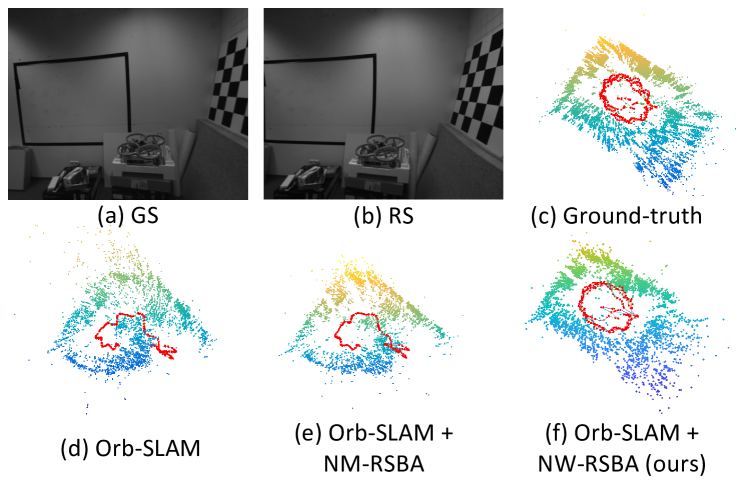
Figure 1: Images were captured at the same time with fast motion with (a) global shutter and (b) rolling shutter in sequence 10 of the TUM-RSVI dataset [21]. (c) classical Orb-SLAM [18] with GS input. (d) classical Orb-SLAM [18] with RS input. (e) Orb-SLAM with NM-RSBA [2]. (f) Orb-SLAM with proposed NW-RSBA.

1.1 Related Work

Video-based Methods. Hedborg et al. [10] use an RS video sequence to solve RSSfM and present an RSBA algorithm under the smooth motion assumption between consecutive frames in [9]. Similarly, Im et al. [11] propose a small motion interpolation-based RSBA algorithm specifically for narrow-baseline RS image sequences. Zhuang et al. [24] further address this setting by presenting 8pt and 9pt linear solvers, which are developed to recover the relative pose of an RS camera that undergoes constant velocity and acceleration motion, respectively. Differently, a spline-based trajectory model to better reformulate the RS camera motion between consecutive frames is proposed by [19].

Unordered RSBA. An unordered image set is the standard input for SfM. Albl et al. [2] address the unordered RSSfM problem and point out the planar degeneracy configuration of RSSfM. Ito et al. [12] attempt to solve RSSfM by establishing an equivalence with self-calibrated SfM based on the pure rotation instantaneous-motion model and affine camera assumption, while the work of [15] draws the equivalence between RSSfM and non-rigid SfM. A camera-based RSBA has been proposed in [14] to simulate the actual camera projection which has the resilience ability against planar degeneracy.

Direct Methods. Unlike the feature-based BA methods that minimize reprojection errors of keypoints, photometric-based BA methods maximize the photometric consistency among each pair of frames instead (e.g. [6, 7]). To handle the RS effect, the works of [13] and [20] present direct semi-dense and direct spare SLAM pipelines, respectively.

1.2 Motivations

Although existing works of RSBA have shown promising results, we argue that they generally lead to either highly complex constraints on inputs, overly restrictive motion models, or time-consuming which limit application fields.

More general: 1) Video-based [9, 11, 24, 19] and direct methods [13, 20] that use video sequence as input are often not desirable to be processed frame by frame which results in high computational power requirements. 2) The unordered image set is the typical input for classical SfM pipeline (e.g. [23]). 3) Even the BA step in current popular SLAM systems (e.g. [18]) only optimizes keyframes instead of all the consecutive frames.

More effective: [2] points out that when the input images are taken with similar readout directions, RSBA fails to recover structure and motion. The proposed solution is simply to avoid the degeneracy configurations by taking images with perpendicular readout directions. This solution considerably limits the use in common scenarios.

More efficient: GSBA argumentation with the RS motion model has been reported as time-consuming, except for the work of [9] to accelerate video-based RSBA. However, the acceleration of unordered RSBA has never been addressed in the existing works [2, 12, 14, 15].

In summary, an accurate and fast solution to unordered images RSBA without camera motion assumptions, readout direction is still missing. Such a method would be a vital step in the potential widespread deployment of 3D vision with RS imaging systems.

1.3 Contribution

In this paper, we present a novel RSBA solution and tackle the challenges that remained in the previous works. To this end, 1) we investigate the influence of normalization to the image point on RSBA performance and show its advantages. 2) Then we present an analytical model for the visual residual covariance, which can standardize the reprojection error during BA, consequently improving the overall accuracy. 3) Moreover, the combination of Normalization and covariance standardization Weighting in RSBA (NW-RSBA) can avoid common planar degeneracy without constraining the capture manner. 4) Besides, we propose its acceleration strategy based on the sparsity of the Jacobian matrix and Schur complement. As shown in Fig. 1 that NW-RSBA can be easily implemented and plugin GSSfM and GSSLAM as RSSfM and RSSLAM solutions.

In summary, the main contributions of this paper are:

• We first thoroughly investigate image point normalization’s influence on RSBA and propose a probability-based weighting algorithm in the cost function to improve RSBA performance. We apply these two insights in the proposed RSBA framework and demonstrate its acceleration strategy.

• The proposed RSBA solution NW-RSBA can easily plugin multiple existing GSSfM and GSSLAM solutions to handle the RS effect. The experiments show that NW-RSBA provides more accurate results and $10\times$ speedup over the existing works. Besides, it avoids planar degeneracy with the usual capture manner.

2 Formulation of RSBA

We formulate the problem of RSBA and provide a brief description of three RSBA methods in existing works. Since this section does not contain our contributions, we give only the necessary details to follow the paper.

$\bullet$ Direct-measurement-based RS model: Assuming a 3D point $\mathbf{P}_{i}=[X_{i}\ Y_{i}\ Z_{i}]$ is observed by a RS camera $j$ represented by measurement $\mathbf{m}_{i}^{j}$ in the image domain. The projection from 3D world to the image can be defined as:

$${\mathbf{m}_{i}^{j}}=\begin{bmatrix}u_{i}^{j}&v_{i}^{j}\end{bmatrix}^{\top}=\Pi(\mathbf{K}{\mathbf{P}^{c}}_{i}^{j}),$$ (1)

$${\mathbf{P}^{c}}_{i}^{j}=[{X^{c}}_{i}^{j}\ {Y^{c}}_{i}^{j}\ {Z^{c}}_{i}^{j}]^{\top}=\mathbf{R}^{j}(v_{i}^{j})\mathbf{P}_{i}+\mathbf{t}^{j}(v_{i}^{j}),$$ (2)

where $\Pi([X\ Y\ Z]^{\top})=\frac{1}{Z}[X\ Y]^{\top}$ is the perspective division and $\mathbf{K}$ is the camera intrinsic matrix [8]. $\mathbf{R}^{j}(v_{i}^{j})\in\mathbf{SO}({3})$ and $\mathbf{t}^{j}(v_{i}^{j})\in\mathbb{R}^{3}$ define the camera rotation and translation respectively when the row index of measurement $v_{i}^{j}$ is acquired. Assuming constant camera motion during frame capture, we can model the instantaneous-motion as:

$$\mathbf{R}^{j}(v_{i}^{j})=(\mathbf{I}+[\bm{\omega}^{j}]_{\times}v_{i}^{j})\mathbf{R}_{0}^{j},\qquad\mathbf{t}^{j}(v_{i}^{j})=\mathbf{t}_{0}^{j}+\mathbf{d}^{j}v_{i}^{j},$$ (3)

where $[\bm{\omega}^{j}]_{\times}$ represents the skew-symmetric matrix of vector $\bm{\omega}^{j}$ and $\mathbf{t}_{0}^{j}$, $\mathbf{R}_{0}^{j}$ is the translation and rotation matrix when the first row is observed. While $\mathbf{d}^{j}=[d_{x}^{j},d_{y}^{j},d_{z}^{j}]^{\top}$ is the linear velocity vector and $\bm{\omega}^{j}=[\omega_{x}^{j},\omega_{y}^{j},\omega_{z}^{j}]^{\top}$ is the angular velocity vector. Such model was adopted by [4, 2, 15]. Notice that RS instantaneous-motion is a function of $v_{i}^{j}$, which we named the direct-measurement-based RS model.

$\bullet$ Normalized-measurement-based RS model: By assuming a pre-calibrated camera, one can transform an image measurement $\mathbf{m}_{i}^{j}$ with $\mathbf{K}$ to the normalized measurement $[{\mathbf{q}_{i}^{j}}^{\top},1]^{\top}=\mathbf{K}^{-1}[{\mathbf{m}_{i}^{j}}^{\top},1]^{\top}$. Thus, the projection model and camera instantaneous-motion become:

$$\mathbf{q}_{i}^{j}=\begin{bmatrix}c_{i}^{j}&r_{i}^{j}\end{bmatrix}^{\top}=\Pi(\mathbf{R}^{j}(r_{i}^{j})\mathbf{P}_{i}+\mathbf{t}^{j}(r_{i}^{j})),$$ (4)

$$\mathbf{R}^{j}(r_{i}^{j})=(\mathbf{I}+[\bm{\omega}^{j}]_{\times}r_{i}^{j})\mathbf{R}_{0}^{j},\quad\mathbf{t}^{j}(r_{i}^{j})=\mathbf{t}^{j}_{0}+\mathbf{d}^{j}r_{i}^{j}.$$ (5)

In contrast to the direct-measurement-based RS model, $\mathbf{t}_{0}^{j}$ and $\mathbf{R}_{0}^{j}$ are the translation and rotation when the optical centre row is observed. $\bm{\omega}^{j}$, $\mathbf{d}^{j}$ are scaled by camera focal length. We name such model the normalized-measurement-based RS model, which was used in [9, 2, 12, 24].

$\bullet$ Rolling Shutter Bundle Adjustment: The non-linear least squares optimizers are used to find a solution $\bm{\theta}^{*}$ including camera poses $\mathbf{R}^{*},\mathbf{t}^{*}$, instantaneous-motion $\bm{\omega}^{*},\mathbf{d}^{*}$ and 3D points $\mathbf{P}^{*}$ by minimizing the reprojection error $\mathbf{e}_{i}^{j}$ from point $i$ to camera $j$ over all the camera index in set $\mathcal{F}$ and corresponding 3D points index in subset $\mathcal{P}_{j}$:

(1) Direct-measurement-based RSBA: [5] uses the direct-measurement-based RS model and compute the reprojection error as: $\mathbf{e}_{i}^{j}=\mathbf{m}_{i}^{j}-\Pi(\mathbf{K}(\mathbf{R}^{j}(v_{i}^{j})\mathbf{P}_{i}+\mathbf{t}^{j}(v_{i}^{j})))$. We name this strategy DM-RSBA.

(2) Normalized-measurement-based RSBA: [2] uses the normalized-measurement-based RS model and compute the reprojection error as: $\mathbf{e}_{i}^{j}=\mathbf{q}_{i}^{j}-\Pi(\mathbf{R}^{j}(r_{i}^{j})\mathbf{P}_{i}+\mathbf{t}^{j}(r_{i}^{j}))$. We name this strategy NM-RSBA.

(3) Direct-camera-base RSBA: Lao et al. [14] argue both DM-RSBA and NM-RSBA can not simulate the actual projection. So [14] proposes a camera-based approach that uses camera pose and instantaneous motion to compute the reprojection without using either $v_{i}^{j}$ or $r_{i}^{j}$. We name this strategy DC-RSBA.

3 Methodology

In this section, we present a novel RSBA algorithm called normalized weighted RSBA (NW-RSBA). The main idea is to use measurement normalization (section 3.1) and covariance standardization weighting (section 3.2) jointly during the optimization. Besides, we provide a two-stage Schur complement strategy to accelerate NW-RSBA in section 3.3. The pipeline of NW-RSBA is shown in Alg. 3. The main differences between NW-RSBA and existing methods [5, 2, 14] are summarized in Tab. 1.

1

Input : Initial rolling shutter camera poses and points as state vector $\bm{\theta}$. Observed point measurement in normalized image coordinate.

Output : Refined state vector $\bm{\theta}^{*}$

2 while (not reach max iteration) and (not satisfy stopping criteria) do

3      

4      for  Each camera $j\in\mathcal{F}$ do

5             for  Each point $i\in\mathcal{P}_{j}$ do

6                   Calculate error $\mathbf{\hat{e}}^{j}_{i}$ using Eq.( 13);

7                   Construct matrix $\mathbf{J}^{j}_{i}$ (supplemental material);

8                   Parallel connect $\mathbf{J}^{j}_{i}$ to $\mathbf{J}$;

9                   Stack $\mathbf{\hat{e}}^{j}_{i}$ into $\mathbf{\hat{e}}$;

10                  

11             end for

12            

13       end for

14      Solve equation $\mathbf{J}^{\top}\mathbf{J}\bm{\delta}=-\mathbf{J}^{\top}\mathbf{\hat{e}}$ using Alg. 6;

15       Update state vector $\bm{\theta}$ using $\bm{\delta}$;

16      

17 end while

Algorithm 1 Normalized Weighted RSBA

Table 1: Comparison of the proposed NW-RSBA and existing general unordered RSBA methods [5, 2, 14]. D: Direct measurement; N: normalized measurement; M-based: measurement-based projection model; C-based: camera-based projection model.

	DM-RSBA[5]	NM-RSBA[2]	DC-RSBA[14]	NW-RSBA
Normalization	D	N	D	N
Reprojecting computation	M-based	M-based	C-based	M-based
Analytical Jacobian	$\times$	$\surd$	$\times$	$\surd$
BA acceleration	$\times$	$\times$	$\times$	$\surd$

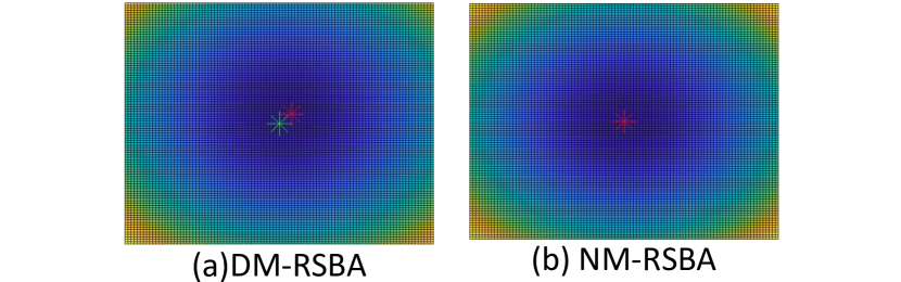
Figure 2: Reprojection loss surface of (a) DM-RSBA [5] and (b) NM-RSBA [2] under the same configuration. The x-axis and y-axis are $d_{x}^{j}$ and $d_{y}^{j}$ of camera motion, respectively. The * are the ground truth solutions while the * are the minimums in loss surfaces.

3.1 Measurement Normalization

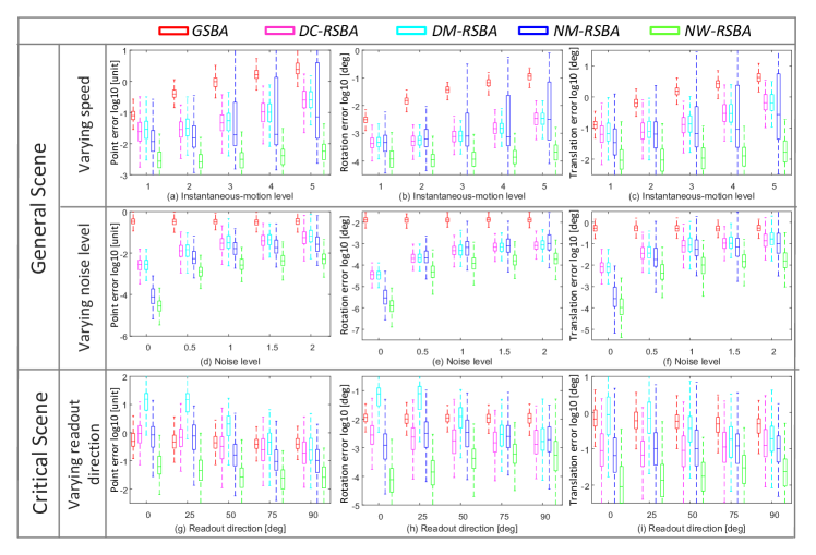
Figure 12: Camera pose ($2^{\text{nd}}$ and $3^{\text{rd}}$ columns) and reconstruction ($1^{\text{st}}$ column) errors of GSBA, DC-RSBA, DM-RSBA, NM-RSBA and NW-RSBA with increasing angular and linear velocity ($1^{\text{st}}$ row) and noise levels in the image ($2^{\text{nd}}$ row) in general scenes, also with increasing readout directions in degeneracy scene ($3^{\text{rd}}$ row).

To the best of our knowledge, no prior research has investigated the influence of normalization on RSBA performance. Thus, we conduct a synthetic experiment to evaluate the impact of normalization by comparing the performances of DM-RSBA [5] and NM-RSBA [2]. The results in Fig. 12 show that the normalization significantly improves the RSBA accuracy. The improvement comes from the more precise instantaneous-motion approximation of low-order Taylor expansion in NM-RSBA. In DM-RSBA, the errors on the image plane induced by the approximate have the same directions and grow exponentially with the increase of the row index. Thus, the optimizer will shift the solution away from the ground truth to equally average the error among all observations. In contrast, the error distribution in NM-RSBA is inherently symmetrical due to the opposite direction with the row varying from the optical center, thus exhibiting significantly lower bias. A synthetic example shown in Fig. 2 verifies our insight that NM-RSBA has an unbiased local minimum over DM-RSBA.

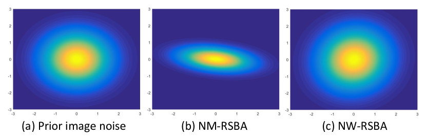
Figure 3: Simulated distributions of (a) prior Gaussian image noise, error term of (b) NM-RSBA [2], and the proposed (c) NW-RSBA.

3.2 Normalized Weighted RSBA

Based on the measurement normalization, we further present a normalized weighted RSBA (NW-RSBA) by modelling image noise covariance.
$\bullet$ Weighting the reprojection error: In contrast to existing works [5, 2, 14], we consider the image noise in RSBA by weighting the squared reprojection error with the inverse covariance matrix of the error, which is also known as standardization of the error terms [22]. Thus the cost function in Eq. (6) becomes:

$$\bm{\theta}^{*}=\mathop{\arg\min}_{\bm{\theta}}\sum_{j\in\mathcal{F}}\sum_{i\in\mathcal{P}_{j}}\textrm{}{\mathbf{e}_{i}^{j}}^{\top}{\mathbf{\Sigma}_{i}^{j}}^{-1}{\mathbf{e}_{i}^{j}},$$ (7)

where $\mathbf{e}_{i}^{j}$ is the reprojection error computed by normalized-measurement-based approach described in Eq. (4). By assuming the image measurement $\mathbf{q}_{i}^{j}$ follows a prior Gaussian noise: $\mathbf{n}_{i}^{j}\sim\mathcal{N}(0,\mathbf{W\Sigma W}^{\top})$, the newly introduced covariance matrix of the error ${\mathbf{\Sigma}_{i}^{j}}$ is defined as follows (proof in the supplemental material):

$$\mathbf{\Sigma}_{i}^{j}=\mathbf{C}_{i}^{j}\mathbf{W}\mathbf{\Sigma}\mathbf{W}^{\top}{\mathbf{C}_{i}^{j}}^{\top},$$ (8)

$$\mathbf{W}=\begin{bmatrix}1/f_{x}&0\\ 0&1/f_{y}\end{bmatrix},$$ (10)

where $\mathbf{C}_{i}^{j}$ and $\mathbf{W}$ are $2\times 2$ auxiliary matrices. $f_{x}$ and $f_{y}$ are focal lengths.

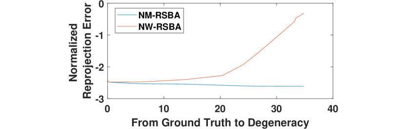
Figure 4: The normalized reprojection error comparison between our proposed method NW-RSBA and NM-RSBA [2] along the degeneracy process.

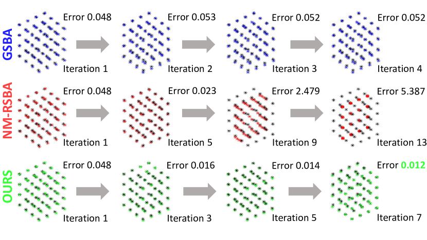
Figure 5: Analysis of the degeneracy in synthetic cube scene captured by five cameras with parallel readout direction. The reconstruction of NM-RSBA [2] (red) collapses to the plane gradually while NW-RSBA (green) provides the most accurate result.

$\bullet$ Advantages of noise covariance weighting: Note that the standardisation in Eq. (7) scaling every term by its inverse covariance matrix ${\mathbf{\Sigma}_{i}^{j}}^{-1}$, so that all terms end up with isotropic covariance [22]. In Fig. 3, we visualize the influence of error terms standardization, which re-scales the prior covariance ellipse back to a unit one. We interpret the re-weighting standardization leads two advantages:

(1) More accurate: With the re-weighting standardization in Eq. (7), features with a high variance which means a high probability of a large reprojection error, are offered less confidence to down-weighting their influence on the total error. Synthetic experiments in section F.1 demonstrate it outperforms NM-RSBA under various noise levels.

(2) Handle planar degeneracy: Though the proposed NW-RSBA uses measurement-based projection during degeneracy, it still provides stable BA results and even outperforms C-RSBA with the noise covariance weighting. As demonstrated in [2], under the planar degeneracy configuration, the y-component of the reprojection error will reduce to zero, which denotes that the covariance matrix holds a zero element in the y direction. NW-RSBA explicitly modeled the error covariance and standardized it to isotropy. Thus, the proposed method exponentially amplifies the error during degeneracy, as shown in Fig. 4, and prevents the continuation of the decline from ground truth to the degenerated solution (proofs can be found in the supplemental material). A synthetic experiment shown in Fig. 5 verifies that NM-RSBA easily collapses into degeneracy solutions while NW-RSBA provide stable result and outperforms the GSBA.

$\bullet$ Jacobian of NW-RSBA: For more convenient optimization, we reformulate covariance matrix $\mathbf{\Sigma}_{i}^{j}$ as a standard least square problem using decomposition:

$${\mathbf{\Sigma}_{i}^{j}}^{-1}={\mathbf{C}_{i}^{j}}^{-\top}\mathbf{W}^{-\top}\mathbf{\Sigma}^{-\frac{1}{2}}\mathbf{\Sigma}^{-\frac{1}{2}}\mathbf{W}^{-1}{\mathbf{C}_{i}^{j}}^{-1}.$$ (11)

By substituting Eq. (11) into (7), we get a new cost function:

$$\bm{\theta}^{*}=\mathop{\arg\min}_{\bm{\theta}}\sum_{j\in\mathcal{F}}\sum_{i\in\mathcal{P}_{j}}\textrm{}{{\mathbf{\hat{e}}^{j\top}_{i}}}{\mathbf{\hat{e}}^{j}_{i}},$$ (12)

$$\noindent\text{where},\begin{aligned} {\mathbf{\hat{e}}_{i}^{j}}=\mathbf{\Sigma}^{-\frac{1}{2}}\mathbf{W}^{-1}{\mathbf{C}_{i}^{j}}^{-1}\mathbf{e}_{i}^{j}.\end{aligned}$$ (13)

We derive the analytical Jacobian matrix of ${\mathbf{\hat{e}}^{j}_{i}}$ in Eq. (12) using the chain rule in the supplemental material.

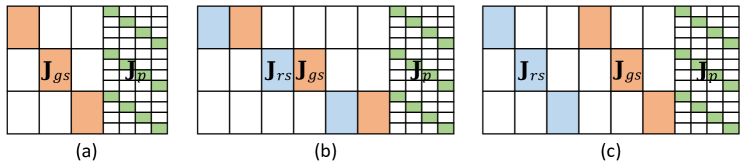
Figure 6: Example Jacobian matrices with 4 points and 3 cameras in (a) GSBA, RSBA with (b) series and (c) parallel connection.

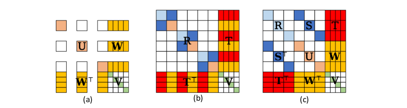
Figure 7: Example Hessian matrices with 4 points and 3 cameras in (a) GSBA, RSBA with(b) series and (c) parallel connection.

1

Input : Jacobian matrix $\mathbf{J}$ and weighted error vector $\mathbf{\hat{e}}$

Output : Update state vector $\bm{\delta}$

2 Compute Schur complement matrix $\textbf{S}_{p}$ and $\textbf{S}_{rs}$ using Eq. (LABEL:equation:Sp) and (17);

3 Compute auxiliary vectors $\textbf{t}^{*}$ and $\textbf{u}^{*}$using Eq. (19) and (18);

Solve Eq. (20) cascadingly:

• Get $\bm{\delta}_{rs}$ by solving $\mathbf{S}_{rs}\bm{\delta}_{rs}=-\mathbf{t}^{*}$;

Get $\bm{\delta}_{gs}$ by solving $\mathbf{U}^{*}\bm{\delta}_{gs}=-\textbf{u}^{*}-\mathbf{S}^{*\top}\bm{\delta}_{rs}$;

Get $\bm{\delta}_{p}$ by solving $\mathbf{V}\bm{\delta}_{p}=-\mathbf{v}-\mathbf{T}^{\top}\bm{\delta}_{rs}-\mathbf{W}^{\top}\bm{\delta}_{gs}$;

Stack $\bm{\delta}_{gs}$, $\bm{\delta}_{rs}$, $\bm{\delta}_{p}$ into $\bm{\delta}$;

8

Algorithm 2 Solve the normal equation using two-stage Schur complement

3.3 NW-RSBA Acceleration

Based on the sparsity of the Jacobian, the marginalization [22, 16] with Schur complement has achieved significant success in accelerating GSBA. However, the acceleration strategy has never been addressed for the general unordered RSBA in [5, 2, 14]. As shown in Fig. 6(b)(c), we can organize the RSBA Jacobian in two styles:

(1) Series connection: By connecting camera pose and instantaneous-motion in the Jacobian matrix (Fig. 7(b)) as an entirety, we can use the one-stage Schur complement technique [16] to marginalize out the 3D point and compute the update state vector for $\mathbf{R},\mathbf{t},\bm{\omega},\mathbf{d}$ first, followed by back substitution for update state vector of points $\mathbf{P}$.

(2) Parallel connection: Due to the independence between camera pose and instantaneous-motion in the Jacobian matrix (Fig. 7(c)), we propose a two-stage Schur complement strategy to accelerate RSBA. When solving the non-linear least square problem (e.g. Gauss-Newton), the approximate Hessian matrix for Eq. (12) is defined as

$$\mathbf{J} =\begin{bmatrix}\mathbf{J}_{rs}&\mathbf{J}_{gs}&\mathbf{J}_{p}\end{bmatrix}=\begin{bmatrix}\frac{\partial{\mathbf{\hat{e}}}}{\partial\mathbf{x}_{rs}}&\frac{\partial{\mathbf{\hat{e}}}}{\partial\mathbf{x}_{gs}}&\frac{\partial{\mathbf{\hat{e}}}}{\partial\mathbf{x}_{p}}\end{bmatrix},$$ (14a)

$$\mathbf{\hat{e}} =\left[\begin{Bmatrix}\mathbf{\hat{e}}_{i}^{j}\end{Bmatrix}\right],\quad\mathbf{x}_{gs}=\begin{bmatrix}\begin{Bmatrix}\mathbf{R}^{j}\end{Bmatrix}&\begin{Bmatrix}\mathbf{t}^{j}\end{Bmatrix}\end{bmatrix},$$ (14b-1)

$$\mathbf{x}_{rs} =\begin{bmatrix}\begin{Bmatrix}\bm{\omega}^{j}\end{Bmatrix}&\begin{Bmatrix}\mathbf{d}^{j}\end{Bmatrix}\end{bmatrix},\quad\mathbf{x}_{p}=\left[\begin{Bmatrix}\mathbf{P}_{i}\end{Bmatrix}\right],$$ (14b-2)

where $\mathbf{R}$, $\mathbf{U}$, $\mathbf{V}$, $\mathbf{S}$, $\mathbf{T}$ and $\mathbf{W}$ are submatrices computed by the derivations $\mathbf{J}_{rs}$, $\mathbf{J}_{gs}$ and $\mathbf{J}_{p}$. As Alg. 6 shown that the two-stage Schur complement strategy consists of 3 steps:

$\triangleright$ Step 1: Construct normal equation. In each iteration, using this form of the Jacobian and corresponding state vectors and the error vector, the normal equation follows

where $\bm{\delta}_{gs}$, $\bm{\delta}_{rs}$ and $\bm{\delta}_{p}$ are the update state vectors to $\mathbf{x}_{gs}$, $\mathbf{x}_{rs}$, and $\mathbf{x}_{p}$, while $\mathbf{t}$, $\mathbf{u}$, and $\mathbf{v}$ are the corresponding descent direction. Such formed normal equations show a block sparsity, suggesting that we can efficiently solve it.

$\triangleright$ Step 2: Construct Schur complement. We construct two-stage Schur complements $\mathbf{S}_{p}$, $\mathbf{S}_{rs}$ and two auxiliary vectors $\mathbf{u}^{*}$ and $\mathbf{t}^{*}$ to Eq. (15) as

$$\mathbf{S}_{rs} =\mathbf{R}^{*}-\mathbf{S}^{*}{\mathbf{U}^{*}}^{-1}{\mathbf{S}^{*}}^{\top},$$ (17)

$$\mathbf{u}^{*} =\mathbf{u}-\mathbf{W}\mathbf{V}^{-1}\mathbf{v},$$ (18)

$$\textbf{t}^{*} =\textbf{t}-\textbf{T}\textbf{V}^{-1}\textbf{v}-\textbf{S}^{*}\textbf{U}^{*-1}\textbf{u}^{*}.$$ (19)

$\triangleright$ Step 3: Orderly solve $\bm{\delta}_{gs}$, $\bm{\delta}_{rs}$ and $\bm{\delta}_{p}$. Based on $\mathbf{S}_{p}$, $\mathbf{S}_{rs}$, $\mathbf{u}^{*}$ and $\mathbf{t}^{*}$, we reformulate the normal equation as

$$\begin{bmatrix}\mathbf{S}_{rs}&\mathbf{0}&\mathbf{0}\\ \mathbf{S}^{*\top}&{\mathbf{U}^{*}}&\mathbf{0}\\ {\mathbf{T}^{\top}}&{\mathbf{W}^{\top}}&{\mathbf{V}}\end{bmatrix}\begin{bmatrix}\bm{\delta}_{rs}\\ \bm{\delta}_{gs}\\ \bm{\delta}_{p}\end{bmatrix}=-\begin{bmatrix}\mathbf{t}^{*}\\ \mathbf{u}^{*}\\ \mathbf{v}\end{bmatrix},$$ (20)

which enables us to compute $\bm{\delta}_{rs}$ first, and then back substitutes the results to get $\bm{\delta}_{gs}$. Finally, we can obtain $\bm{\delta}_{p}$ based on the $3^{\text{rd}}$ row of Eq. (20).

3.4 Implementation

We follow Alg. 3 to implement the proposed NW-RSBA in C++. The implemented NW-RSBA can serve as a little module and can be easily plug-in such context:

$\bullet$ RS-SfM: We augment VisualSFM [23] by shifting the incremental GSBA pipeline with the proposed NW-RSBA.

$\bullet$ RS-SLAM: We augment Orb-SLAM [18] by replacing the local BA and full BA modules with NW-RSBA.

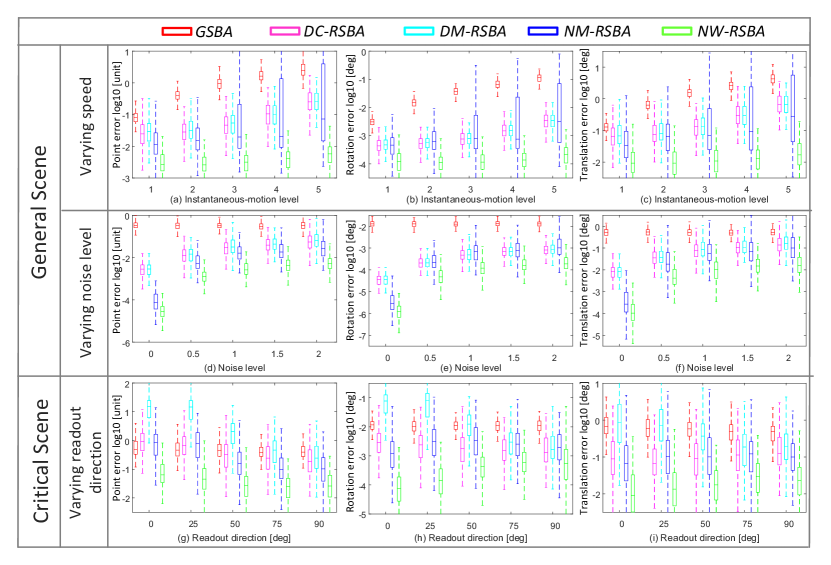
Figure 8: Camera pose ($2^{\text{nd}}$ and $3^{\text{rd}}$ columns) and reconstruction ($1^{\text{st}}$ column) errors of GSBA, DC-RSBA, DM-RSBA, NM-RSBA and NW-RSBA with increasing angular and linear velocity ($1^{\text{st}}$ row) and noise levels in the image ($2^{\text{nd}}$ row) in a general scene, also with increasing readout directions in a degeneracy scene ($3^{\text{rd}}$ row).

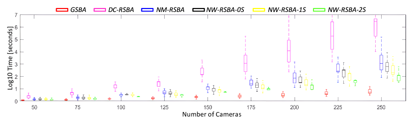
Figure 9: Time cost of GSBA [16], DC-RSBA [14], NM-RSBA [2], NW-RSBA-0S (without Schur complement), NW-RSBA-1S (one-stage Schur complement to Jacobian matrices with series connection), and proposed NW-RSBA-2S (two-stage Schur complement to Jacobian matrices with parallel connection) with increasing camera number and fixed point number.

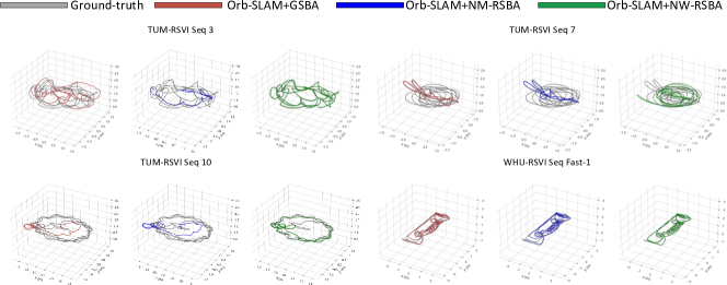
Figure 10: Ground truth and trajectories estimated by GSBA [16], NM-RSBA [2] and proposed NW-RSBA after Sim(3) alignment on 3 sequences from TUM-RSVI [21] and 1 sequence from WHU-RSVI [3] datasets.

4 Experimental Evaluation

In our experiments, the proposed method is compared to three state-of-the-art unordered RSBA solutions:1) GSBA: SBA [16]. 2) DC-RSBA: direct camera-based RSBA [14]. 3) DM-RSBA: direct measurement-based RSBA [5]. 4) NM-RSBA: normalized-measurement-based RSBA [2]. 5) NW-RSBA: proposed normalized weighted RSBA.

4.1 Synthetic Data

Settings and metrics. We simulate $5$ RS cameras located randomly on a sphere pointing at a cubical scene. We compare all methods by varying the speed, the image noise, and the readout direction. The results are obtained after collecting the errors over 300 trials per epoch. We measure the reconstruction errors and pose errors.

Results. 1) Varying Speed. The results in Fig. 12(a)(b)(c) show that the estimated errors of GSBA grow with speed while DC-RSBA, DM-RSBA and NM-RSBA achieve better results with slow kinematics. The proposed NW-RSBA provides the best results under all configurations. 2) Varying Noise Level. In Fig. 12(d)(e)(f), GSBA shows better robustness to noise but with lower accuracy than RS methods. The proposed NW-RSBA achieves the best performance with all noise levels. 3) Varying Readout Direction. We evaluate five methods with varying readout directions of the cameras by increasing the angle from parallel to perpendicular. Fig. 12(g)(h)(i) show that under a small angle, the reconstruction error of DM-RSBA, DC-RSBA and DM-RSBA grow dramatically even bigger than GSBA, suggesting a degenerated solution. In contrast, NW-RSBA provides stable results under all settings, even with the parallel readout direction.

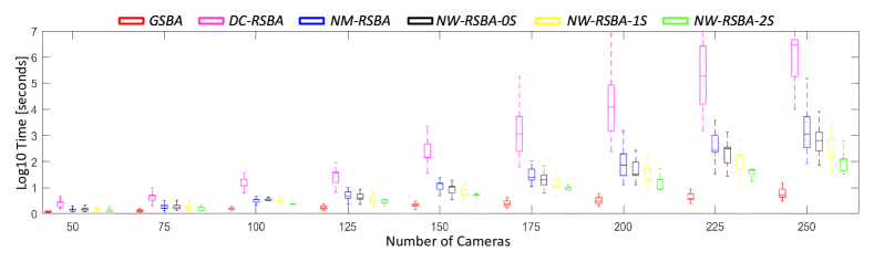
Figure 13: Time cost of GSBA [16], DC-RSBA [14], NM-RSBA [2], NW-RSBA-0S (without Schur complement), NW-RSBA-1S (one-stage Schur complement to Jacobian matrices with series connection), and proposed NW-RSBA-2S (two-stage Schur complement to Jacobian matrices with parallel connection) with increasing camera number.

Runtime. As shown in Fig. 13 that without analytical Jacobian, DC-RSBA is the slowest one while the proposed NW-RSBA achieves similar efficiency as NM-RSBA. However, by using acceleration strategies, NW-RSBA-1S and NW-RSBA-2S reduce the overall runtime. Note that NW-RSBA-2S achieves an order of magnitude faster than NM-RSBA.

4.2 Real Data

Datasets and metrics. We compare all the RSBA methods in two publicly available RS datasets: WHU-RSVI [3] dataset, TUM-RSVI [21] dataset. In this section, we use three evaluation metrics, namely ATE $e_{\text{ate}}$ (absolute trajectory error) [21], tracking duration $\underline{DUR}$ (the ratio of the successfully tracked frames out of the total frames) and real-time factor $\epsilon$ (sequence’s actual duration divided by the algorithm’s processing time).

Table 2: Statistics of 10 sequences from TUM-RSVI [21] and 2 sequences from WHU-RSVI [3] datasets. The realtime factor $\epsilon$ and tracking duration $\underline{DUR}$ of Orb-SLAM, Orb-SALM+NM-RSBA [2], and proposed Orb-SLAM+NW-RSBA.

Seq	Duration [s]	length [m]	Realtime factor $\epsilon$ $\uparrow$ $\mid$ Tracking duration $\underline{DUR}$ $\uparrow$
			Orb-SLAM [18]	Orb-SLAM +NM-RSBA [2]	Orb-SLAM +NW-RSBA
#1	40	46	1.47 $\mid$ 0.50	1.48 $\mid$ 0.28	1.38 $\mid$ 1
#2	27	37	1.51 $\mid$ 0.90	1.40 $\mid$ 0.81	1.40 $\mid$ 1
#3	50	44	1.47 $\mid$ 0.58	1.41 $\mid$ 0.36	1.39 $\mid$ 1
#4	38	30	1.61 $\mid$ 1	1.35 $\mid$ 1	1.56 $\mid$ 1
#5	85	57	1.51 $\mid$ 1	1.28 $\mid$ 1	1.38 $\mid$ 1
#6	43	51	1.47 $\mid$ 0.76	1.37 $\mid$ 0.76	1.38 $\mid$ 1
#7	39	45	1.61 $\mid$ 0.89	1.47 $\mid$ 0.97	1.49 $\mid$ 1
#8	53	46	1.56 $\mid$ 0.79	1.37 $\mid$ 0.96	1.35 $\mid$ 1
#9	45	46	1.61 $\mid$ 0.14	1.51 $\mid$ 0.23	1.55 $\mid$ 0.42
#10	54	41	1.56 $\mid$ 0.29	1.46 $\mid$ 0.29	1.47 $\mid$ 1
t1-fast	28	50	1.92 $\mid$ 1	1.51 $\mid$ 1	1.81 $\mid$ 1
t2-fast	29	53	1.92 $\mid$ 1	1.40 $\mid$ 1	1.67 $\mid$ 1

Table 3: Absolute trajectory error (ATE) of different RSBA methods after $\text{Sim}(3)$ alignment to ground truth. The best results are shown in green. Since some methods will lose tracking without processing the whole sequence, thus we highlight the background of each cell with different colours depending on its corresponding DUR value. Specifically, $\textit{\text@underline{DUR}}>0.9$, $0.5<\textit{\text@underline{DUR}}\leqslant 0.9$ and $\textit{\text@underline{DUR}}\leqslant 0.5$ are highlighted in light green, cyan, and orange.

Input	Methods		ATE$\downarrow$
			TUM-RSVI [21]											WHU-RSVI [3]
			#1	#2	#3	#4	#5	#6	#7	#8	#9	#10		t1-fast	t2-fast
GS data	Orb-SLAM [18]		0.015	0.013	0.018	0.107	0.030	0.013	0.054	0.053	0.020	0.024		0.044	0.008
RS data	Orb-SLAM [18]		0.059	0.100	0.411	0.126	0.055	0.044	0.217	0.218	0.176	0.373		0.237	0.018
	Orb-SLAM+NM-RSBA [2]		0.115	0.088	0.348	0.120	0.062	0.060	0.251	0.246	0.156	0.307		0.204	0.030
	Orb-SLAM+NW-RSBA (ours)		0.011	0.008	0.031	0.071	0.034	0.008	0.260	0.115	0.028	0.108		0.054	0.012

4.2.1 RSSLAM

We compare the performance of conventional GS-based Orb-SLAM [18] versus augmented versions with NM-RSBA [2] and proposed NW-RSBA on 12 RS sequences.

Real-time factor and tracking duration. Tab. 2 shows the statistics about 12 RS sequences and the performance of three approaches run on an AMD Ryzen 7 CPU. The results verify that all three methods achieve real-time performance. One can also confirm that the proposed Orb-SLAM+NW-RSBA is slower than Orb-SLAM by a factor roughly around $1.2$ but is slightly faster than Orb-SLAM+NM-RSBA. As for tracking duration, Orb-SLAM and Orb-SLAM+NM-RSBA [2] fail with an average $\underline{DUR}<0.5$ in most sequences once the camera moves aggressively enough. In contrast, the proposed Orb-SLAM+NW-RSBA achieves completed tracking with $\underline{DUR}=1$ in almost all sequences.

Absolute trajectory error. The ATE results on WHU-RSVI and TUM-RSVI datasets demonstrate that the proposed Orb-SLAM+NW-RSBA is superior to Orb-SLAM and Orb-SLAM+NM-RSBA when dealing with RS effect. Qualitatively, this is clearly visible in Figs. 1 and 14. The sparse 3D reconstructions look much cleaner for Orb-SLAM+NW-RSBA and close to the ground truth. The quantitative difference also becomes apparent in Tab. 3. Orb-SLAM+NW-RSBA outperforms Orb-SLAM and Orb-SLAM+NM-RSBA both in terms of accuracy and stability.

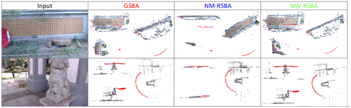
Figure 11: Three-view graph of reconstructions using SfM pipeline with GSBA [16], NM-RSBA [2] and proposed NW-RSBA.

Table 4: Quantitative ablation study of RSSfM on TUM-RSVI [21] and WHU-RSVI [3] datasets. ATE: absolute trajectory error of estimated camera pose in meters ($m$), Runtime: time cost in seconds ($s$). Best and second best results are shown in green and blue respectively.

Ablation	Approach	ATE ($m$)	Runtime ($s$)
	GSBA [16]	0.210	2.9
	DC-RSBA [14]	0.016	1302
No normalization & weighting	DM-RSBA [5]	0.023	740
No weighting	NM-RSBA [2]	0.020	15.8
No normalization	W-RSBA	0.013	16.1
No Schur complement	NW-RSBA-0S	0.007	16.9
with 1-stage Schur complement	NW-RSBA-1S		13.0
Consolidated	NW-RSBA-2S		9.8

4.2.2 RSSfM

Quantitative Ablation Study. We randomly choose 8 frames from each of the 12 RS sequences to generate 12 unordered SfM datasets and evaluate the RSBA performance via average ATE and runtime. Besides, we ablate the NW-RSBA and compare quantitatively with related approaches. The results are presented in Tab. 4. The baseline methods’ performance show that NW-RSBA obtains ATE of 0.007, which is half of the second best method DC-RSBA and nearly $3\%$ of GSBA. The removal of normalization from proposed NW-RSBA adversely increases ATE up to $100\%$. The removal of covariance weighting from NW-RSBA adversely impacts the camera pose estimation quality with ATE growth from 0.007 to 0.020. We believe that covariance weighting helps BA leverage the RS effect and random image noise better. We ablate the consolidated NW-RSBA-2S to NW-RSBA-0S by removing the proposed 2-stage Schur complement strategy and compare to NW-RSBA-1S. The increases from 9.8s to 13.0s and 16.9s is observed for average runtime. Despite the fact NW-RSBA-2S is slower than GSBA by a factor of 3, but still 2 times faster than NM-RSBA, 2 orders of magnitude faster than DC-RSBA and DM-RSBA.

Qualitative Samples. We captured two datasets using a smartphone camera and kept the same readout direction, which is a degeneracy configuration in RSBA and will quickly lead to a planar degenerated solution for NM-RSBA [2]. As shown in Fig. 11 that NW-RSBA works better in motion and 3D scene estimation while GSBA [16] obtains a deformed reconstruction. Specifically, the sparse 3D reconstructions and recovered trajectories of NW-RSBA look much cleaner and smoother than the ones from GSBA. NM-RSBA reconstructs 3D scenes which collapse into a plane since the datasets contain only one readout direction. In contrast, NW-RSBA provides correct reconstructions. The results also verify our discussion in section 3.2 that error covariance weighting can handle the planar degeneracy.

5 Conclusion

This paper presents a novel RSBA solution without any assumption on camera image manner and type of video input. We explain the importance of conducting normalization and present a weighting technique in RSBA, which leads to normalized weighted RSBA. Extensive experiments in real and synthetic data verify the effectiveness and efficiency of the proposed NW-RSBA method.

Acknowledgements. This work is supported by the National Key R&D Program of China (No. 2022ZD0119003), Nature Science Foundation of China (No. 62102145), and Jiangxi Provincial 03 Special Foundation and 5G Program (Grant No. 20224ABC03A05).

Appendix A Proof of Reprojection Error Covariance

In this section, we perform a detailed proof of reprojection error covariance. Firstly, we decompose a normalized image measurement point $\mathbf{q}_{i}^{j}=\begin{bmatrix}c&r\end{bmatrix}^{\top}$ into a perfect normalized image measurement point $\tilde{\mathbf{q}}_{i}^{j}=\begin{bmatrix}\tilde{c}&\tilde{r}\end{bmatrix}^{\top}$ and a normalized image Gaussian measurement noise $\begin{bmatrix}n_{c}&n_{r}\end{bmatrix}^{\top}$:

$$\begin{bmatrix}c&r\end{bmatrix}^{\top}=\begin{bmatrix}\tilde{c}&\tilde{r}\end{bmatrix}^{\top}+\begin{bmatrix}n_{c}&n_{r}\end{bmatrix}^{\top},$$ (21)

with,

$$\begin{bmatrix}n_{c}&n_{r}\end{bmatrix}^{\top}\sim\mathcal{N}(0,\mathbf{W\Sigma}\mathbf{W}^{\top}),$$ (22)

$$\mathbf{W}=\begin{bmatrix}1/f_{x}&0\\ 0&1/f_{y}\end{bmatrix},$$ (23)

where $\mathbf{\Sigma}$ is the prior Gaussian measurement noise and $f_{x}\ f_{y}$ are the x-axis and y-axis focal length respectively. Then we can substitute Eq. (21) to the normalized measurement based reprojection cost function as:

where $\Pi(\mathbf{R}^{j}(\tilde{r}_{i}^{j}+n_{r})\mathbf{P}_{i}+\mathbf{t}^{j}(\tilde{r}_{i}^{j}+n_{r}))$ can be linearized using the Taylor first order approximation:

$$\Pi(\mathbf{R}^{j}(\tilde{r}_{i}^{j}+n_{r})\mathbf{P}_{i}+\mathbf{t}^{j}(\tilde{r}_{i}^{j}+n_{r}))$$ (25)

$$\approx \begin{bmatrix}\tilde{c}_{i}^{j}\\ \tilde{r}_{i}^{j}\end{bmatrix}+\frac{\partial\Pi(\mathbf{R}^{j}({r}_{i}^{j})\mathbf{P}_{i}+\mathbf{t}^{j}({r}_{i}^{j}))}{\partial n_{r}}n_{r}.$$

Then by substituting Eq. (25) into Eq. (24), we have

By applying the chain rule of derivation, we can get the analytical formulation of matrix $\mathbf{C}_{i}^{j}$.

with,

$$\frac{\partial\Pi(\mathbf{R}^{j}({r}_{i}^{j})\mathbf{P}_{i}+\mathbf{t}^{j}({r}_{i}^{j}))}{\partial{\mathbf{P}^{c}}_{i}^{j}}={\begin{bmatrix}\frac{1}{{{Z^{c}}_{i}^{j}}}&0\\ 0&\frac{1}{{{Z^{c}}_{i}^{j}}}\\ \frac{-{{X^{c}}_{i}^{j}}}{{{Z^{c}}_{i}^{j}}^{2}}&\frac{-{{Y^{c}}_{i}^{j}}}{{{Z^{c}}_{i}^{j}}^{2}}\end{bmatrix}}^{\top},$$ (28)

$$\frac{\partial{\mathbf{P}^{c}}_{i}^{j}}{\partial n_{r}}=[\bm{\omega}^{j}]_{\times}\mathbf{R}^{j}\mathbf{P}_{i}+\mathbf{d}^{j}.$$ (29)

By substituting Eq. (27) into Eq. (26), we can get analytical formulation:

where ${\mathbf{P}^{c}}_{i}^{j}={\begin{bmatrix}{X^{c}}_{i}^{j}&{Y^{c}}_{i}^{j}&{Z^{c}}_{i}^{j}\end{bmatrix}}^{\top}=\mathbf{R}^{j}({r}_{i}^{j})\mathbf{P}_{i}+\mathbf{t}^{j}({r}_{i}^{j})$ is the world point $\mathbf{P}_{i}$ in camera $j$ coordinates. Combining Eq. (22) with Eq. (26), we prove that $\mathbf{{e}}_{i}^{j}$ follows a weighted Gaussian distribution:

$$\mathbf{{e}}_{i}^{j}\sim\mathcal{N}(0,\mathbf{C}_{i}^{j}\mathbf{W}\mathbf{\Sigma}\mathbf{W}^{\top}{\mathbf{C}_{i}^{j}}^{\top}).$$ (31)

Appendix B Analytical Jacobian matrix Derivation

In this section, we provide a detailed derivation of the analytical Jacobian matrix used in our proposed NW-RSBA solution.

B.1 Jacobian Matrix Parameterization

To derive the analytical Jacobian matrix of Eq. (35), we use ${\bm{\xi}_{i}^{j}}\in\mathbf{so}({3})$ to parametrize ${\mathbf{R}_{i}^{j}}\in\mathbf{SO}({3})$. These two representations can be transformed to each other by Rodrigues formulation ${\mathbf{R}_{i}^{j}}=\mathbf{Exp}(\bm{\xi}_{i}^{j})$ and ${\bm{\xi}_{i}^{j}}=\mathbf{Log}(\mathbf{R}_{i}^{j})$, which are defined as:

$${\mathbf{R}} =\mathbf{Exp}(\bm{\xi})$$ (32)

$$=\mathbf{I}+\frac{sin(\left\|\bm{\xi}\right\|)}{\left\|\bm{\xi}\right\|}\bm{\xi}^{\wedge}+\frac{1-cos(\left\|\bm{\xi}\right\|)}{{\left\|\bm{\xi}\right\|}^{2}}{(\bm{\xi}^{\wedge})}^{2}.$$

$${\bm{\xi}} =\mathbf{Log}(\mathbf{R})$$ (33)

$$=\frac{\bm{\theta}}{2sin(\bm{\theta})}{(\mathbf{R}-\mathbf{R}^{\top})}^{\vee},$$

with,

$$\bm{\theta}=arccos((tr(\mathbf{R})-1)/2),$$ (34)

where ${\wedge}$ is the skew-symmetric operator that can transform a vector to the corresponding skew-symmetric matrix. Besides, ${\vee}$ is the inverse operator.

B.2 Partial Derivative of Reprojection error

Recall the normalized weighted error term, which is defined as:

$${{\mathbf{\hat{e}}}_{i}^{j}}=\mathbf{\Sigma}^{-\frac{1}{2}}{{\mathbf{W}}^{-1}{{\mathbf{C}_{i}^{j}}}^{-1}\mathbf{e}_{i}^{j}}.$$ (35)

Then we can get five atomic partial derivatives of $\partial{{\mathbf{\hat{e}}_{i}^{j}}}$ over $\partial{{\mathbf{P}_{i}}}$, $\partial\bm{\xi}^{j}$, ${\partial\mathbf{t}^{j}}$, ${\partial\bm{\omega}^{j}}$ and ${\partial\mathbf{d}^{j}}$ as:

with,

$$\frac{\partial{\mathbf{e}_{i}^{j}}}{\partial{\mathbf{P}^{c}}_{i}^{j}} =-\begin{bmatrix}\frac{1}{{{Z}^{c}}_{i}^{j}}&0&-\frac{{{X}^{c}}_{i}^{j}}{({{Z}^{c}}_{i}^{j})^{2}}\\ 0&\frac{1}{{{Z}^{c}}_{i}^{j}}&-\frac{{{Y}^{c}}_{i}^{j}}{({{Z}^{c}}_{i}^{j})^{2}}\\ \end{bmatrix},$$ (41)

$$\frac{\partial{\mathbf{P}^{c}}_{i}^{j}}{\partial\mathbf{P}_{i}} =(\mathbf{I}+[\bm{\omega}^{j}]_{\times}{{r}_{i}^{j}}){\mathbf{R}^{j}},$$ (42)

$$\frac{\partial{\mathbf{P}^{c}}_{i}^{j}}{\partial\bm{\xi}^{j}} =-(\mathbf{I}+[\bm{\omega}^{j}]_{\times}{r}_{i}^{j})[{\mathbf{R}^{j}}\mathbf{P}_{i}]_{\times},$$ (43)

$$\frac{\partial{\mathbf{P}^{c}}_{i}^{j}}{\partial{\mathbf{t}^{j}}} =[\mathbf{I}]_{3\times 3},$$ (44)

$$\frac{\partial{\mathbf{P}^{c}}_{i}^{j}}{\partial\bm{\omega}^{j}} =-r_{i}^{j}[{\mathbf{R}^{j}}\mathbf{P}_{i}]_{\times},$$ (45)

$$\frac{\partial{\mathbf{P}^{c}}_{i}^{j}}{\partial{\mathbf{d}^{j}}} ={r}_{i}^{j}[\mathbf{I}]_{3\times 3},$$ (46)

where ${\mathbf{C}_{i}^{j}}(1)$ and ${\mathbf{C}_{i}^{j}}(2)$ represents the first and second row of matrix ${\mathbf{C}_{i}^{j}}$ respectively.

We further need to derive the partial derivatives of $\partial{{\mathbf{C}_{i}^{j}}(.)^{-\top}}$ over $\partial{{\mathbf{P}_{i}}}$, $\partial\bm{\xi}^{j}$, ${\partial\mathbf{t}^{j}}$, ${\partial\bm{\omega}^{j}}$ and ${\partial\mathbf{d}^{j}}$ in Eq. (36 - 40). Recall the $\mathbf{C}_{i}^{j}$ and $\mathbf{W}$ definition in Eq. (30) and Eq. (23). For convenience, we define the following two intermediate variables:

$$\bm{\gamma}_{i}^{j} ={\begin{bmatrix}\frac{1}{{{Z^{c}}_{i}^{j}}}&0\\ 0&\frac{1}{{{Z^{c}}_{i}^{j}}}\\ \frac{-{{X^{c}}_{i}^{j}}}{{{Z^{c}}_{i}^{j}}^{2}}&\frac{-{{Y^{c}}_{i}^{j}}}{{{Z^{c}}_{i}^{j}}^{2}}\end{bmatrix}}^{\top},$$ (47)

$$\bm{\delta}_{i}^{j} =[\bm{\omega}^{j}]_{\times}{\mathbf{R}^{j}}\mathbf{P}_{i}+\mathbf{d}^{j}.$$ (48)

Then we can rewrite Eq. (30) as:

$$\mathbf{C}_{i}^{j}=\begin{bmatrix}1&0\\ 0&1\end{bmatrix}-\bm{\gamma}_{i}^{j}\bm{\delta}_{i}^{j}\begin{bmatrix}0&1\end{bmatrix}=\begin{bmatrix}1&-\bm{\gamma}_{i}^{j}\bm{\delta}_{i}^{j}\\ 0&1-\bm{\gamma}_{i}^{j}\bm{\delta}_{i}^{j}\end{bmatrix},$$ (49)

and its inverse formulation as:

$${\mathbf{C}_{i}^{j}}^{-1}=\begin{bmatrix}1&\frac{\bm{\gamma}_{i}^{j}\bm{\delta}_{i}^{j}}{1-\bm{\gamma}_{i}^{j}\bm{\delta}_{i}^{j}}\\ 0&\frac{1}{1-\bm{\gamma}_{i}^{j}\bm{\delta}_{i}^{j}}\end{bmatrix}.$$ (50)

Then we can derive the partial derivative as:

$$\frac{\partial{{\mathbf{C}_{i}^{j}}(1)^{-\top}}}{\partial\mathbf{P}_{i}}=\begin{bmatrix}[0]_{1\times 3}\\ \frac{(1-\bm{\beta})\frac{\partial{\bm{\alpha}_{i}^{j}}}{\partial{\mathbf{P}_{i}}}+\bm{\alpha}\frac{\partial{\bm{\beta}_{i}^{j}}}{\partial{\mathbf{P}_{i}}}}{(1-\bm{\beta}_{i}^{j})^{2}}\end{bmatrix},$$ (51)

$$\frac{\partial{\mathbf{C}_{i}^{j}(2)}^{-\top}}{\partial\mathbf{P}_{i}}=\begin{bmatrix}[0]_{1\times 3}\\ \frac{\frac{\partial{\bm{\beta}_{i}^{j}}}{\partial{\mathbf{P}_{i}}}}{(1-\bm{\beta}_{i}^{j})^{2}}\end{bmatrix},$$ (52)

$$\frac{\partial{{\mathbf{C}_{i}^{j}}(1)^{-\top}}}{\partial{\bm{\xi}}^{j}}=\begin{bmatrix}[0]_{1\times 3}\\ \frac{(1-\bm{\beta}_{i}^{j})\frac{\partial{\bm{\alpha}_{i}^{j}}}{\partial{\bm{\xi}^{j}}}+\bm{\alpha}_{i}^{j}\frac{\partial{\bm{\beta}_{i}^{j}}}{\partial{\bm{\xi}^{j}}}}{(1-\bm{\beta}_{i}^{j})^{2}}\end{bmatrix},$$ (53)

$$\frac{\partial{\mathbf{C}_{i}^{j}(2)}^{-\top}}{\partial{\bm{\xi}}^{j}}=\begin{bmatrix}[0]_{1\times 3}\\ \frac{\frac{\partial{\bm{\beta}_{i}^{j}}}{\partial{{\bm{\xi}}^{j}}}}{(1-\bm{\beta}_{i}^{j})^{2}}\end{bmatrix},$$ (54)

$$\frac{\partial{{\mathbf{C}_{i}^{j}}(1)^{-\top}}}{\partial\mathbf{t}^{j}}=\begin{bmatrix}[0]_{1\times 3}\\ \frac{(1-\bm{\beta}_{i}^{j})\frac{\partial{\bm{\alpha}_{i}^{j}}}{\partial{\mathbf{t}^{j}}}+\bm{\alpha}_{i}^{j}\frac{\partial{\bm{\beta}_{i}^{j}}}{\partial{\mathbf{t}^{j}}}}{(1-\bm{\beta}_{i}^{j})^{2}}\end{bmatrix},$$ (55)

$$\frac{\partial{\mathbf{C}_{i}^{j}(2)}^{-\top}}{\partial\mathbf{t}^{j}}=\begin{bmatrix}[0]_{1\times 3}\\ \frac{\frac{\partial{\bm{\beta}_{i}^{j}}}{\partial{\mathbf{t}^{j}}}}{(1-\bm{\beta}_{i}^{j})^{2}}\end{bmatrix},$$ (56)

$$\frac{\partial{{\mathbf{C}_{i}^{j}}(1)^{-\top}}}{\partial\bm{\omega}^{j}}=\begin{bmatrix}[0]_{1\times 3}\\ \frac{(1-\bm{\beta}_{i}^{j})\frac{\partial{\bm{\alpha}_{i}^{j}}}{\partial{\bm{\omega}^{j}}}+\bm{\alpha}_{i}^{j}\frac{\partial{\bm{\beta}_{i}^{j}}}{\partial{\bm{\omega}^{j}}}}{(1-\bm{\beta}_{i}^{j})^{2}}\end{bmatrix},$$ (57)

$$\frac{\partial{\mathbf{C}_{i}^{j}(2)}^{-\top}}{\partial\bm{\omega}^{j}}=\begin{bmatrix}[0]_{1\times 3}\\ \frac{\frac{\partial{\bm{\beta}_{i}^{j}}}{\partial{{\bm{\omega}}^{j}}}}{(1-\bm{\beta}_{i}^{j})^{2}}\end{bmatrix},$$ (58)

$$\frac{\partial{{\mathbf{C}_{i}^{j}}(1)^{-\top}}}{\partial\mathbf{d}^{j}}=\begin{bmatrix}[0]_{1\times 3}\\ \frac{(1-\bm{\beta}_{i}^{j})\frac{\partial{\bm{\alpha}_{i}^{j}}}{\partial{\mathbf{d}^{j}}}+\bm{\alpha}_{i}^{j}\frac{\partial{\bm{\beta}_{i}^{j}}}{\partial{\mathbf{d}^{j}}}}{(1-\bm{\beta}_{i}^{j})^{2}}\end{bmatrix},$$ (59)

$$\frac{\partial{\mathbf{C}_{i}^{j}(2)}^{-\top}}{\partial\mathbf{d}^{j}}=\begin{bmatrix}[0]_{1\times 3}\\ \frac{\frac{\partial{\bm{\beta}_{i}^{j}}}{\partial{\mathbf{d}^{j}}}}{(1-\bm{\beta}_{i}^{j})^{2}}\end{bmatrix},$$ (60)

where $\mathbf{C}(1)$ and $\mathbf{C}(2)$ are the first and second row of $\mathbf{C}$ respectively, and two intermediate variables $\bm{\alpha}_{i}^{j}\ \bm{\beta}_{i}^{j}$ are the first and second row of $\bm{\gamma}_{i}^{j}\bm{\delta}_{i}^{j}$ respectively

$$\bm{\gamma}_{i}^{j}\bm{\delta}_{i}^{j}=\begin{bmatrix}\bm{\alpha}_{i}^{j}\\ \bm{\beta}_{i}^{j}\end{bmatrix}.$$ (61)

Finally we have to derive the partial derivative of $\partial{\bm{\alpha}_{i}^{j}}$ and $\partial{\bm{\beta}_{i}^{j}}$ over $\partial{{\mathbf{P}_{i}}}$, $\partial\bm{\xi}^{j}$, ${\partial\mathbf{t}^{j}}$, ${\partial\bm{\omega}^{j}}$ and ${\partial\mathbf{d}^{j}}$ in Eq. (51 - 60):

$$\frac{\partial(\bm{\gamma}_{i}^{j}\bm{\delta}_{i}^{j})}{\partial\mathbf{P}_{i}}=\bm{\gamma}_{i}^{j}\frac{\partial\bm{\delta}_{i}^{j}}{\partial{\mathbf{P}_{i}}}+\begin{bmatrix}{\bm{\delta}_{i}^{j}}^{\top}\frac{\partial\bm{\gamma}_{i}^{j}(1)^{\top}}{\partial{\mathbf{P}^{c}}_{i}^{j}}\frac{\partial{\mathbf{P}^{c}}_{i}^{j}}{\partial{\mathbf{P}_{i}}}\\ {\bm{\delta}_{i}^{j}}^{\top}\frac{\partial\bm{\gamma}_{i}^{j}(2)^{\top}}{\partial{\mathbf{P}^{c}}_{i}^{j}}\frac{\partial{\mathbf{P}^{c}}_{i}^{j}}{\partial{\mathbf{P}_{i}}}\end{bmatrix},$$ (62)

$$\frac{\partial(\bm{\gamma}_{i}^{j}\bm{\delta}_{i}^{j})}{\partial{\bm{\xi}}^{j}}=\mathbf{\gamma}_{i}^{j}\frac{\partial\bm{\delta}_{i}^{j}}{\partial{\bm{\xi}^{j}}}+\begin{bmatrix}{\bm{\delta}_{i}^{j}}^{\top}\frac{\partial\bm{\gamma}_{i}^{j}(1)^{\top}}{\partial{\mathbf{P}^{c}}_{i}^{j}}\frac{\partial{\mathbf{P}^{c}}_{i}^{j}}{\partial{\bm{\xi}^{j}}}\\ {\bm{\delta}_{i}^{j}}^{\top}\frac{\partial\bm{\gamma}_{i}^{j}(2)^{\top}}{\partial{\mathbf{P}^{c}}_{i}^{j}}\frac{\partial{\mathbf{P}^{c}}_{i}^{j}}{\partial{\bm{\xi}^{j}}}\end{bmatrix},$$ (63)

$$\frac{\partial(\bm{\gamma}_{i}^{j}\bm{\delta}_{i}^{j})}{\partial\mathbf{t}^{j}}=\bm{\gamma}_{i}^{j}\frac{\partial\bm{\delta}_{i}^{j}}{\partial{\mathbf{t}^{j}}}+\begin{bmatrix}{\bm{\delta}_{i}^{j}}^{\top}\frac{\partial\bm{\gamma}_{i}^{j}(1)^{\top}}{\partial{\mathbf{P}^{c}}_{i}^{j}}\frac{\partial{\mathbf{P}^{c}}_{i}^{j}}{\partial{\mathbf{t}^{j}}}\\ {\bm{\delta}_{i}^{j}}^{\top}\frac{\partial\bm{\gamma}_{i}^{j}(2)^{\top}}{\partial{\mathbf{P}^{c}}_{i}^{j}}\frac{\partial{\mathbf{P}^{c}}_{i}^{j}}{\partial{\mathbf{t}^{j}}}\end{bmatrix},$$ (64)

$$\frac{\partial(\bm{\gamma}_{i}^{j}\bm{\delta}_{i}^{j})}{\partial\bm{\omega}^{j}}=\bm{\gamma}_{i}^{j}\frac{\partial\bm{\delta}_{i}^{j}}{\partial{\bm{\omega}^{j}}}+\begin{bmatrix}{\bm{\delta}_{i}^{j}}^{\top}\frac{\partial\bm{\gamma}_{i}^{j}(1)^{\top}}{\partial{\mathbf{P}^{c}}_{i}^{j}}\frac{\partial{\mathbf{P}^{c}}_{i}^{j}}{\partial{\bm{\omega}^{j}}}\\ {\bm{\delta}_{i}^{j}}^{\top}\frac{\partial\bm{\gamma}_{i}^{j}(2)^{\top}}{\partial{\mathbf{P}^{c}}_{i}^{j}}\frac{\partial{\mathbf{P}^{c}}_{i}^{j}}{\partial{\bm{\omega}^{j}}}\end{bmatrix},$$ (65)

$$\frac{\partial(\bm{\gamma}_{i}^{j}\bm{\delta}_{i}^{j})}{\partial\mathbf{d}^{j}}=\bm{\gamma}_{i}^{j}\frac{\partial\bm{\delta}_{i}^{j}}{\partial{\mathbf{d}^{j}}}+\begin{bmatrix}{\bm{\delta}_{i}^{j}}^{\top}\frac{\partial\bm{\gamma}_{i}^{j}(1)^{\top}}{\partial{\mathbf{P}^{c}}_{i}^{j}}\frac{\partial{\mathbf{P}^{c}}_{i}^{j}}{\partial{\mathbf{d}^{j}}}\\ {\bm{\delta}_{i}^{j}}^{\top}\frac{\partial\bm{\gamma}_{i}^{j}(2)^{\top}}{\partial{\mathbf{P}^{c}}_{i}^{j}}\frac{\partial{\mathbf{P}^{c}}_{i}^{j}}{\partial{\mathbf{d}^{j}}}\end{bmatrix},$$ (66)

with,

$$\frac{\partial\bm{\gamma}_{i}^{j}(1)^{\top}}{\partial{\mathbf{P}^{c}}_{i}^{j}} =\begin{bmatrix}0&0&-\frac{1}{{{Z^{c}}_{i}^{j}}^{2}}\\ 0&0&0\\ -\frac{1}{{{Z^{c}}_{i}^{j}}^{2}}&0&\frac{2{{X^{c}}_{i}^{j}}}{{{Z^{c}}_{i}^{j}}^{3}}\end{bmatrix},$$ (67)

$$\frac{\partial\bm{\gamma}_{i}^{j}(2)^{\top}}{\partial{\mathbf{P}^{c}}_{i}^{j}} =\begin{bmatrix}0&0&0\\ 0&0&-\frac{1}{{{Z^{c}}_{i}^{j}}^{2}}\\ 0&-\frac{1}{{{Z^{c}}_{i}^{j}}^{2}}&\frac{2{{Y^{c}}_{i}^{j}}}{{{Z^{c}}_{i}^{j}}^{3}}\end{bmatrix},$$ (68)

$$\frac{\partial\bm{\delta}_{i}^{j}}{\partial{\mathbf{P}_{i}}} =[\bm{\omega}^{j}]_{\times}\mathbf{R}^{j},$$ (69)

$$\frac{\partial\bm{\delta}_{i}^{j}}{\partial{\bm{\xi}^{j}}} =[\bm{\omega}^{j}]_{\times}[{\mathbf{R}^{j}}\mathbf{P}_{i}]_{\times},$$ (70)

$$\frac{\partial\bm{\delta}_{i}^{j}}{\partial{\mathbf{t}^{j}}} =[0]_{3\times 3},$$ (71)

$$\frac{\partial\bm{\delta}_{i}^{j}}{\partial{\bm{\omega}^{j}}} =-[{\mathbf{R}^{j}}\mathbf{P}_{i}]_{\times},$$ (72)

$$\frac{\partial\bm{\delta}_{i}^{j}}{\partial{\mathbf{d}^{j}}} =[\mathbf{I}]_{3\times 3}.$$ (73)

Appendix C The proof of degeneracy resilience ability

As proved in [2], under the planar degeneracy configuration, the y-component of the reprojection error will reduce to zero. To say it in another way, the noise perturbation along the y-component of the observation will not be reflected in the y-component of the reprojection error (remains at zero). The reprojection error covariance matrix must have a zero variance in the y-coordinate of its values according to the definition of covariance. We prove this theoretically in the following.

In correspondence with notations in the manuscript, we first define ${\mathbf{P}^{g}}_{i}^{j}=[{X^{g}}_{i}^{j}\ {Y^{g}}_{i}^{j}\ {Z^{g}}_{i}^{j}]^{\top}=\mathbf{R}_{0}^{j}\mathbf{P}_{i}+\mathbf{t}_{0}^{j}$ and it can be related with ${\mathbf{P}^{c}}_{i}^{j}$ as $[\bm{\omega}^{j}]_{\times}\mathbf{R}^{j}_{0}\mathbf{P}_{i}+\mathbf{d}^{j}=({\mathbf{P}^{c}}_{i}^{j}-{\mathbf{P}^{g}}_{i}^{j})\ /\ {{v}_{i}^{j}}$. Then we rewrite the Eq. (30):

Under the degeneracy configuration, the observed point will project to the plane $y=0$ in the camera coordinate. We then substitute the degeneracy condition ${Y^{g}}_{i}^{j}=0,{Z^{g}}_{i}^{j}={Z^{c}}_{i}^{j},{v}_{i}^{j}={Y^{c}}_{i}^{j}/{Z^{c}}_{i}^{j}$ into Eq.(74). It can be verified that the lower right component of $\mathbf{C}_{i}^{j}$ reduces to zero, which means that the y-coordinate variance in the reprojection error covariance matrix will reduce to zero.

Based on the explicitly modeled reprojection error covariance, we can decompose its inverse form and then reweight the reprojection error Eq.(11-13), which will result an isotropy covariance (Fig. 3). The corresponding weight will rapidly approach infinite during the degeneracy process since the y-coordinate variance gradually reduces to zero. As a result, the reweighted reprojection error will grow exponentially, which will prevent the continuation of the degeneracy. The error of NM-RSBA decreases gradually during the degeneracy process, while NW-RSBA grows exponentially and converges around the ground truth.

Appendix D The equivalent between Normalized DC-RSBA and NW-RSBA

In this section, we provide an equivalent proof and illustrate the deep connection between the Normalized DC-RSBA and proposed NW-RSBA method.

D.1 Pre-definition

Recall the Eq. (26), we define a new vector $\bm{\chi}_{i}^{j}$ for convenience:

$$\bm{\chi}_{i}^{j} =\frac{\partial\Pi(\mathbf{R}^{j}(r_{i}^{j})\mathbf{P}_{i}+\mathbf{t}^{j}(r_{i}^{j}))}{\partial n_{r}}$$ (75)

$$=\frac{\partial\Pi(\mathbf{R}^{j}(r_{i}^{j})\mathbf{P}_{i}+\mathbf{t}^{j}(r_{i}^{j}))}{\partial{r}_{i}^{j}},$$

then we can reformulate Eq. (30) as:

$$\mathbf{C}_{i}^{j} =\begin{bmatrix}1&0\\ 0&1\end{bmatrix}-\frac{\partial\Pi(\mathbf{R}^{j}(r_{i}^{j})\mathbf{P}_{i}+\mathbf{t}^{j}(r_{i}^{j}))}{\partial n_{r}}\begin{bmatrix}0&1\end{bmatrix}$$ (76)

$$=\begin{bmatrix}1&-{\bm{\chi}_{i}^{j}}(1)\\ 0&1-{\bm{\chi}_{i}^{j}}(2)\end{bmatrix},$$

where ${\bm{\chi}_{i}^{j}}(1)\ {\bm{\chi}_{i}^{j}}(2)$ are the first and second row of ${\bm{\chi}_{i}^{j}}$, and its inverse formulation is defined as:

$${\mathbf{C}_{i}^{j}}^{-1}=\begin{bmatrix}1&\frac{{\bm{\chi}_{i}^{j}}(1)}{1-{\bm{\chi}_{i}^{j}}(2)}\\ 0&\frac{1}{1-{\bm{\chi}_{i}^{j}}(2)}\end{bmatrix}.$$ (77)

Then we can define a new rectified image coordinate vector $\begin{bmatrix}{c_{i}^{j}}^{"}&{r_{i}^{j}}^{"}\end{bmatrix}^{\top}$ which represents the virtual image point after weighting.

$$\begin{bmatrix}{c}_{i}^{j}\\ {r}_{i}^{j}\end{bmatrix}-\begin{bmatrix}{c_{i}^{j}}^{"}\\ {r_{i}^{j}}^{"}\end{bmatrix}={\mathbf{C}_{i}^{j}}^{-1}(\begin{bmatrix}{c}_{i}^{j}\\ {r}_{i}^{j}\end{bmatrix}-\begin{bmatrix}{c_{i}^{j}}^{{}^{\prime}}\\ {r_{i}^{j}}^{{}^{\prime}}\end{bmatrix}),$$ (78)

where ${\begin{bmatrix}{c_{i}^{j}}^{{}^{\prime}}&{r_{i}^{j}}^{{}^{\prime}}\end{bmatrix}}^{\top}$ is the projection image point with image measurement ${\begin{bmatrix}{c_{i}^{j}}&{r_{i}^{j}}\end{bmatrix}}^{\top}$, which is defined as:

$${\begin{bmatrix}{c_{i}^{j}}^{{}^{\prime}}&{r_{i}^{j}}^{{}^{\prime}}\end{bmatrix}}^{\top}=\Pi(\mathbf{R}^{j}(r_{i}^{j})\mathbf{P}_{i}+\mathbf{t}^{j}(r_{i}^{j})).$$ (79)

Our goal is to prove that using rectified coordinates as the observed image point will project on the same image point with the normalized measurement-based projection. We can summarize such equivalent as the following equation:

$$\begin{bmatrix}{c_{i}^{j}}^{"}&{r_{i}^{j}}^{"}\end{bmatrix}^{\top}=\Pi(\mathbf{R}^{j}({r_{i}^{j}}^{"})\mathbf{P}_{i}+\mathbf{t}^{j}({r_{i}^{j}}^{"})).$$ (80)

We follow the schedule that firstly solves the Eq. (78) to get the rectified image coordinate vector $\begin{bmatrix}{c_{i}^{j}}^{"}&{r_{i}^{j}}^{"}\end{bmatrix}^{\top}$, use the rectified image coordinate vector in normalized measurement based projection to get the projection point and finally check out whether it is the same.

D.2 New Rectified Image Coordinate Solution

We solve Eq. (78) consequently. Firstly, we solve ${r_{i}^{j}}^{"}$.

$$(1-{\bm{\chi}_{i}^{j}}(2))({r}_{i}^{j}-{r_{i}^{j}}^{"})=({r}_{i}^{j}-{r_{i}^{j}}^{{}^{\prime}}),$$ (81)

$${r_{i}^{j}}^{"} ={r_{i}^{j}}+\frac{{r_{i}^{j}}^{{}^{\prime}}-{r}_{i}^{j}}{1-{\bm{\chi}_{i}^{j}}(2)}$$ (82)

$$={{r}_{i}^{j}}^{{}^{\prime}}+\frac{{\bm{\chi}_{i}^{j}}(2)({r_{i}^{j}}^{{}^{\prime}}-{r}_{i}^{j})}{1-{\bm{\chi}_{i}^{j}}(2)},$$

We then substitute ${r_{i}^{j}}^{"}$ to solve ${c_{i}^{j}}^{"}$.

$$({c}_{i}^{j}-{c_{i}^{j}}^{"})=\frac{{\bm{\chi}_{i}^{j}}(1)}{1-{\bm{\chi}_{i}^{j}}(2)}({r}_{i}^{j}-{r_{i}^{j}}^{{}^{\prime}})+({c}_{i}^{j}-{c_{i}^{j}}^{{}^{\prime}}),$$ (83)

$${c_{i}^{j}}^{"}={c_{i}^{j}}^{{}^{\prime}}+\frac{{\bm{\chi}_{i}^{j}}(1)({r_{i}^{j}}^{{}^{\prime}}-{r}_{i}^{j})}{1-{\bm{\chi}_{i}^{j}}(2)}.$$ (84)

D.3 Proof of equivalent after projection

We then substitute ${r_{i}^{j}}^{"}$ and ${c_{i}^{j}}^{"}$ in normalized measurement based projection.

D.4 Connection between Normalized DC- RSBA and NW-RSBA

From Eq. (85), we can get a such summary that Normalized DC-RSBA is equivalent to the proposed NW-RSBA mathematical. It is amazing to view that although the two formulations are totally different from each other, they both bring in the implicit rolling shutter constraint to optimization. However, although these two methods are equivalent to each other, our proposed NW-RSBA is much easier and faster to solve since we provide detailed analytical Jacobian matrices.

Appendix E Proposed NW-RSBA Algorithm Pipeline

In this section, we provide a detailed bundle adjustment algorithm pipeline with the standard Gauss-Newton least square solver.

List of Algorithms

loa

1

Input: Initial rolling shutter camera poses $\{\mathbf{R}^{1},\mathbf{t}^{1},\bm{\omega}^{1},\mathbf{d}^{1}\}$,…,$\{\mathbf{R}^{j},\mathbf{t}^{j},\bm{\omega}^{j},\mathbf{d}^{j}\}$, points $\mathbf{P}_{1}$,…,$\mathbf{P}_{i}$ as $\bm{\theta}$ and point measurement in normalized image coordinate $\mathbf{q}^{1...j}_{1...i}$

Output: Refined parameters $\bm{\theta}^{*}$

2 while (not reach max iteration) and (not satisfy stopping criteria) do

3      

4      for  Each camera $j\in\mathcal{F}$ do

5             for  Each point $i\in\mathcal{P}_{j}$ do

6                   Calculate weighted reprojection error $\mathbf{\hat{e}}^{j}_{i}$ using Alg. 4;

7                   Construct Jacobian matrix $\mathbf{J}^{j}_{i}$ using Alg. 5;

8                   Parallel connect $\mathbf{J}^{j}_{i}$ to $\mathbf{J}$;

9                   Stack $\mathbf{\hat{e}}^{j}_{i}$ into $\mathbf{\hat{e}}$;

10                  

11             end for

12            

13       end for

14      Solve normal equation $\mathbf{J}^{\top}\mathbf{J}\bm{\delta}=-\mathbf{J}^{\top}\mathbf{\hat{e}}$ using Alg. 6;

15       Update camera poses and points parameters $\bm{\theta}$ using $\bm{\delta}$;

16      

17 end while

Algorithm 3 Normalized Weighted RSBA

1

Input : Rolling shutter camera poses $\{\mathbf{R}^{j},\mathbf{t}^{j},\bm{\omega}^{j},\mathbf{d}^{j}\}$, points $\mathbf{P}_{i}$ and point measurement in normalized image coordinate $\mathbf{q}^{j}_{i}$

Output : Normalized weighted error $\mathbf{\hat{e}}^{j}_{i}$

2 Compute weight matrix $\mathbf{C}^{j}_{i}$ using Eq. (30);

3 Compute standard reprojection error $\mathbf{e}^{j}_{i}$;

4 Return normalized weighted reprojection error $\mathbf{\hat{e}}^{j}_{i}$ using Eq. (35);

5

Algorithm 4 Computation of weighted reprojection error

Input : RS camera poses $\{\mathbf{R}^{j},\mathbf{t}^{j},\bm{\omega}^{j},\mathbf{d}^{j}\}$, points coordinate $\mathbf{P}_{i}$ and point measurement in normalized image coordinate $\mathbf{q}^{j}_{i}$

Output : Jacobian matrix $\mathbf{J}^{j}_{i}$

1

2Calculate $\frac{\partial{\hat{\mathbf{e}}_{i}^{j}}}{\partial\mathbf{P}_{i}}$ using Eq. (36);

3

4Calculate $\frac{\partial{\hat{\mathbf{e}}_{i}^{j}}}{\partial{\bm{\xi}}^{j}}$ using Eq. (37);

5

6Calculate $\frac{\partial{\hat{\mathbf{e}}_{i}^{j}}}{\partial\mathbf{t}^{j}}$ using Eq. (38);

7

8Calculate $\frac{\partial{\hat{\mathbf{e}}_{i}^{j}}}{\partial\bm{\omega}^{j}}$ using Eq. (39);

9

10Calculate $\frac{\partial{\hat{\mathbf{e}}_{i}^{j}}}{\partial\mathbf{d}^{j}}$ using Eq. (40);

11

12Construct

$$\mathbf{J}^{j}_{i} =\begin{bmatrix}\mathbf{J}_{i,rs}^{j}&\mathbf{J}_{i,gs}^{j}&\mathbf{J}_{i,p}^{j}\end{bmatrix}$$

$$=\begin{bmatrix}[\frac{\partial{\hat{\mathbf{e}}_{i}^{j}}}{\partial{\bm{\omega}}^{j}},\frac{\partial{\hat{\mathbf{e}}_{i}^{j}}}{\partial{\mathbf{d}}^{j}}]&[\frac{\partial{\hat{\mathbf{e}}_{i}^{j}}}{\partial{\bm{\xi}}^{j}},\frac{\partial{\hat{\mathbf{e}}_{i}^{j}}}{\partial{\mathbf{t}}^{j}}]&\frac{\partial{\hat{\mathbf{e}}_{i}^{j}}}{\partial{\mathbf{P}}_{i}}\end{bmatrix};$$

Algorithm 5 Computation of Jacobian matrix

1

Input : Jacobian matrix $\mathbf{J}$ and weighted error vector $\mathbf{\hat{e}}$

Output : Updated vector $\bm{\delta}$

2 Compute Schur complement matrix $\textbf{S}_{p}$ and $\textbf{S}_{rs}$;

3 Compute auxiliary vectors $\textbf{t}^{*}$ and $\textbf{u}^{*}$;

4

Solve normal equation cascadingly:

• Get $\bm{\delta}_{rs}$ by solving $\mathbf{S}_{rs}\bm{\delta}_{rs}=-\mathbf{t}^{*}$;

Get $\bm{\delta}_{gs}$ by solving $\mathbf{U}^{*}\bm{\delta}_{gs}=-\textbf{u}^{*}-\mathbf{S}^{*\top}\bm{\delta}_{rs}$;

Get $\bm{\delta}_{p}$ by solving $\mathbf{V}\bm{\delta}_{p}=-\mathbf{v}-\mathbf{T}^{\top}\bm{\delta}_{rs}-\mathbf{W}^{\top}\bm{\delta}_{gs}$;

Stack $\bm{\delta}_{gs}$ $\bm{\delta}_{rs}$ $\bm{\delta}_{p}$ into $\bm{\delta}$;

9

Algorithm 6 Solve the normal equation using two-stage Schur complement

Appendix F Experimental Settings and Evaluation Metrics

In this section, we provide detailed experiment settings and evaluation metrics used in synthetic data experiments and real data experiments.

F.1 Synthetic Data

Experimental Settings. We simulate $5$ RS cameras located randomly on a sphere with a radius of 20 units pointing to a cubical scene with 56 points. The RS image size is 1280 × 1080 px, the focal length is about 1000, and the optical center is at the center of the image domain. We compare all methods by varying the speed, the noise on image measurements, and the readout direction. The results are obtained after collecting the errors over 300 trials each epoch. The default setting is 10 deg/frame and 1 unit/frame for angular and linear velocity, standard covariance noise.

• Varying Speed: We evaluate the accuracy of five approaches against increasing angular and linear velocity from 0 to 20 deg/frame and 0 to 2 units/frame gradually, with random directions.

• Varying Noise Level: We evaluate the accuracy of five approaches against increasing noise level from 0 to 2 pixels.

• Varying Readout Direction: We evaluate the robustness of five methods with an RS critical configuration. Namely, the readout directions of all views are almost parallel. Thus, we vary the readout directions of the cameras from parallel to perpendicular by increasing the angle from 0 to 90 degrees.

• Runtime: We compare the time cost of all methods against increasing the number of cameras from 50 - 250 with a fixed number of points.

Evaluation metrics. In this section, we use three metrics to evaluate the performances, namely reconstruction error, rotation error, and translation error.

• Reconstruction Error $\mathbf{e}_{\text{point}}$: We use the reconstruction error to measure the difference between computed and ground truth 3D points, which is defined as:
  $\mathbf{e}_{\text{point}}={\begin{Vmatrix}\mathbf{P}-\mathbf{P}_{\text{GT}}\end{Vmatrix}}^{2}$.

• Rotation Error $\mathbf{e}_{\text{rot}}$: We utilize the geodesic distance to measure the error between optimized rotation and ground truth. The error is defined as:
  $\mathbf{e}_{\text{rot}}=\arccos((\text{tr}(\mathbf{R}\mathbf{R}_{\text{GT}}^{\top})-1)/2)$.

• Translation Error $\mathbf{e}_{\text{trans}}$: We use normalized inner product distance to measure the error between optimized translation and ground truth, which is defined as:
  $\mathbf{e}_{\text{trans}}=\arccos(\mathbf{t}^{\top}\mathbf{t}_{\text{GT}}/(\left\|\mathbf{t}\right\|\left\|\mathbf{t}_{\text{GT}}\right\|))$.

F.2 Real Data

Datasets Settings. We compare all the RSC methods in the following publicly available RS datasets.

• WHU-RSVI: WHU dataset was published in [3] and provided ground truth synthetic GS images, RS images and camera poses.

• TUM-RSVI: The TUM RS dataset was published in [21] and contained time-synchronized global-shutter, and rolling-shutter images captured by a non-perspective camera rig and ground-truth poses recorded by motion capture system for ten RS video sequences.

Evaluation metrics. In this section, we use three metrics to evaluate the performances, namely absolute trajectory error, tracking duration and real-time factor.

• Absolute trajectory error (ATE). We use the absolute trajectory error (ATE) [21] to evaluate the VO results quantitatively. Given ground truth frame positions $\bar{\mathbf{c}}_{i}\in\mathbb{R}^{3}$ and corresponding Orb-SLAM [18] tracking results $\mathbf{c}_{i}\in\mathbb{R}^{3}$ using corrected sequence by each RSC method. It is defined as

  $$e_{\text{ate}}=\min_{\mathbf{T}\in\text{Sim}(3)}\sqrt{\frac{1}{n}\sum_{i=1}^{n}\left\|\mathbf{T}(\textbf{c}_{i})-\bar{\textbf{c}}_{i}\right\|},$$ (86)

  where $\mathbf{T}\in\text{Sim}(3)$ is a similarity transformation that aligns the estimated trajectory with the ground truth one since the scale is not observable for monocular methods. We run each method 20 times on each sequence to obtain the ATE $e_{\text{ate}}$.

• Tracking duration (DUR). Besides, we find out that some RSC solutions provide the results of corrections that are even worse than the original input RS frames. This leads to failure in tracking and makes Orb-SLAM interrupt before the latest capture frame. Therefore, we use the ratio of the successfully tracked frames out of the total frames DUR as an evaluation metric.

• Realtime factor $\epsilon$. The realtime factor $\epsilon$ is calculated as the sequence’s actual duration divided by the algorithm’s processing time.

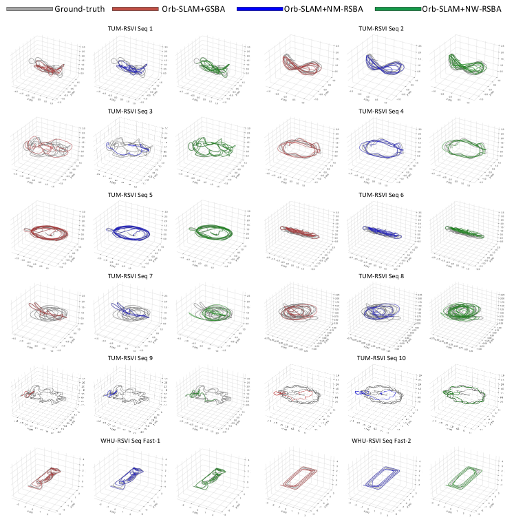
Figure 14: Ground truth and trajectories estimated by GSBA [16], NM-RSBA [2] and proposed NW-RSBA after Sim(3) alignment on 10 sequences from TUM-RSVI [21] and 2 sequences from WHU-RSVI [3] datasets.

References

- [1] Cenek Albl, Zuzana Kukelova, Viktor Larsson, and Tomas Pajdla. Rolling shutter camera absolute pose. PAMI, 2019.
- [2] Cenek Albl, Akihiro Sugimoto, and Tomas Pajdla. Degeneracies in rolling shutter sfm. In ECCV, 2016.
- [3] Like Cao, Jie Ling, and Xiaohui Xiao. The whu rolling shutter visual-inertial dataset. IEEE Access, 8:50771–50779, 2020.
- [4] Yuchao Dai, Hongdong Li, and Laurent Kneip. Rolling shutter camera relative pose: generalized epipolar geometry. In CVPR, 2016.
- [5] Gaspard Duchamp, Omar Ait-Aider, Eric Royer, and Jean-Marc Lavest. A rolling shutter compliant method for localisation and reconstruction. In VISAPP, 2015.
- [6] Jakob Engel, Vladlen Koltun, and Daniel Cremers. Direct sparse odometry. PAMI, 2017.
- [7] Jakob Engel, Thomas Schöps, and Daniel Cremers. Lsd-slam: Large-scale direct monocular slam. In ECCV, 2014.
- [8] Richard Hartley and Andrew Zisserman. Multiple view geometry in computer vision. Cambridge university press, 2003.
- [9] Johan Hedborg, Per-Erik Forssen, Michael Felsberg, and Erik Ringaby. Rolling shutter bundle adjustment. In CVPR, 2012.
- [10] Johan Hedborg, Erik Ringaby, Per-Erik Forssén, and Michael Felsberg. Structure and motion estimation from rolling shutter video. In ICCV Workshops, 2011.
- [11] Sunghoon Im, Hyowon Ha, Gyeongmin Choe, Hae-Gon Jeon, Kyungdon Joo, and In So Kweon. Accurate 3d reconstruction from small motion clip for rolling shutter cameras. PAMI, 2018.
- [12] Eisuke Ito and Takayuki Okatani. Self-calibration-based approach to critical motion sequences of rolling-shutter structure from motion. In CVPR, 2016.
- [13] J. H. Kim, C. Cadena, and I. Reid. Direct semi-dense slam for rolling shutter cameras. In ICRA, 2016.
- [14] Yizhen Lao, Omar Ait-Aider, and Helder Araujo. Robustified structure from motion with rolling-shutter camera using straightness constraint. Pattern Recognition Letters, 2018.
- [15] Yizhen Lao, Omar Ait-Aider, and Adrien Bartoli. Solving rolling shutter 3d vision problems using analogies with non-rigidity. IJCV, 2021.
- [16] Manolis IA Lourakis and Antonis A Argyros. Sba: A software package for generic sparse bundle adjustment. ACM Transactions on Mathematical Software (TOMS), 36(1):1–30, 2009.
- [17] M Meingast, C Geyer, and S Sastry. Geometric models of rolling-shutter cameras. In OMNIVIS, 2005.
- [18] Raul Mur-Artal, Jose Maria Martinez Montiel, and Juan D Tardos. Orb-slam: a versatile and accurate monocular slam system. T-RO, 2015.
- [19] Alonso Patron-Perez, Steven Lovegrove, and Gabe Sibley. A spline-based trajectory representation for sensor fusion and rolling shutter cameras. IJCV, 2015.
- [20] David Schubert, Nikolaus Demmel, Vladyslav Usenko, Jörg Stückler, and Daniel Cremers. Direct sparse odometry with rolling shutter. ECCV, 2018.
- [21] David Schubert, Nikolaus Demmel, Lukas von Stumberg, Vladyslav Usenko, and Daniel Cremers. Rolling-shutter modelling for direct visual-inertial odometry. In IROS, 2019.
- [22] Bill Triggs, Philip F McLauchlan, Richard I Hartley, and Andrew W Fitzgibbon. Bundle adjustment—a modern synthesis. In International workshop on vision algorithms, pages 298–372. Springer, 1999.
- [23] Changchang Wu et al. Visualsfm: A visual structure from motion system. 2011.
- [24] Bingbing Zhuang, Loong-Fah Cheong, and Gim Hee Lee. Rolling-shutter-aware differential sfm and image rectification. In ICCV, 2017.