Better Hardness Results for the Minimum Spanning Tree Congestion Problem

Abstract

In the spanning tree congestion problem, given a connected graph $G$, the objective is to compute a spanning tree $T$ in $G$ that minimizes its maximum edge congestion, where the congestion of an edge $e$ of $T$ is the number of edges in $G$ for which the unique path in $T$ between their endpoints traverses $e$. The problem is known to be ${\mathbb{NP}}$-hard, but its approximability is still poorly understood, and it is not even known whether the optimum solution can be efficiently approximated with ratio $o(n)$. In the decision version of this problem, denoted ${K\!\shortminus\!\textsf{STC}}$, we need to determine if $G$ has a spanning tree with congestion at most $K$. It is known that ${K\!\shortminus\!\textsf{STC}}$ is ${\mathbb{NP}}$-complete for $K\geq 8$, and this implies a lower bound of $1.125$ on the approximation ratio of minimizing congestion. On the other hand, ${3\!\shortminus\!\textsf{STC}}$ can be solved in polynomial time, with the complexity status of this problem for $K\in{\left\{4,5,6,7\right\}}$ remaining an open problem. We substantially improve the earlier hardness results by proving that ${K\!\shortminus\!\textsf{STC}}$ is ${\mathbb{NP}}$-complete for $K\geq 5$. This leaves only the case $K=4$ open, and improves the lower bound on the approximation ratio to $1.2$.

Motivated by evidence that minimizing congestion is hard even for graphs of small constant radius, we consider ${K\!\shortminus\!\textsf{STC}}$ restricted to graphs of radius $2$, and we prove that this variant is ${\mathbb{NP}}$-complete for all $K\geq 6$. Exploring further in this direction, we also examine the variant, denoted ${K\!\shortminus\!\textsf{STC}D}$, where the objective is to determine if the graph has a depth-$D$ spanning three of congestion at most $K$. We prove that ${6\!\shortminus\!\textsf{STC}2}$ is ${\mathbb{NP}}$-complete even for bipartite graphs. For bipartite graphs we establish a tight bound, by also proving that ${5\!\shortminus\!\textsf{STC}2}$ is polynomial-time solvable. Additionally, we complement this result with polynomial-time algorithms for two special cases that involve bipartite graphs and restrictions on vertex degrees.

1 Introduction

Problems involving constructing a spanning tree that satisfies certain requirements are among the most fundamental tasks in graph theory and algorithmics. One such problem is the spanning tree congestion problem, STC for short, that has been studied extensively for many years. In this problem we seek a spanning tree $T$ of a given graph $G$ that roughly approximates the connectivity structure of $G$, in the following sense: Embed $G$ into $T$ by replacing each edge $(u,v)$ of $G$ by the unique $u$-to-$v$ path in $T$. Define the congestion of an edge $e$ of $T$ as the number of such paths that traverse $e$. The objective of STC is to find a spanning tree $T$ in which the maximum edge congestion is minimized.

The general concept of edge congestion was first introduced in 1986, under the name of load factor, as a measure of quality of an embedding of one graph into another [3] (see also the survey in [23]). The problem of computing trees with low congestion was studied by Khuller et al. [15] in the context of solving commodities network routing problems. The trees considered there were not required to be spanning subtrees, but the variant involving spanning trees was also mentioned. In 2003, Ostrovskii provided independently a formal definition of STC and established some fundamental properties of spanning trees with low congestion [20]. Since then, many combinatorial and algorithmic results about this problem have been reported in the literature — we refer the readers to the survey paper by Otachi [21] for more information, most of which is still up-to-date.

As established by Löwenstein [18], STC is ${\mathbb{NP}}$-hard. As usual, this is proved by showing ${\mathbb{NP}}$-completeness of its decision version, where we are given a graph $G$ and an integer $K$, and we need to determine if $G$ has a spanning tree with congestion at most $K$. Otachi et al. [22] strengthened this by proving that the problem remains ${\mathbb{NP}}$-hard even for planar graphs. In [19], STC is proven to be ${\mathbb{NP}}$-hard for chain graphs and split graphs. On the other hand, computing optimal solutions for STC can be achieved in polynomial time for some special classes of graphs: complete $k$-partite graphs, two-dimensional tori [17], outerplanar graphs [5], and two-dimensional Hamming graphs [16].

In our paper, we focus on the decision version of STC where the bound $K$ on congestion is a fixed constant. We denote this variant by ${K\!\shortminus\!\textsf{STC}}$. Several results on the complexity of ${K\!\shortminus\!\textsf{STC}}$ were reported in [22]. For example, the authors of [22] show that ${K\!\shortminus\!\textsf{STC}}$ is decidable in linear time for planar graphs, graphs of bounded treewidth, graphs of bounded degree, and for all graphs when $K=1,2,3$. On the other hand, they show that the problem is ${\mathbb{NP}}$-complete for any fixed $K\geq 10$. In [4], Bodlaender et al. proved that ${K\!\shortminus\!\textsf{STC}}$ is linear-time solvable for graphs in apex-minor-free families and chordal graphs. They also show an improved hardness result of ${K\!\shortminus\!\textsf{STC}}$, namely that it is ${\mathbb{NP}}$-complete for $K\geq 8$, even in the special case of apex graphs that only have one unbounded degree vertex. As stated in [21], the complexity status of ${K\!\shortminus\!\textsf{STC}}$ for $K\in{\left\{4,5,6,7\right\}}$ remains an open problem.

Very little is known about the approximability of STC. The trivial upper bound for the approximation ratio is $n/2$ — this ratio is achieved in fact by any spanning tree [21]. As a direct consequence of the ${\mathbb{NP}}$-completeness of ${8\!\shortminus\!\textsf{STC}}$, there is no polynomial-time algorithm to approximate the optimum spanning tree congestion with a ratio better than $1.125$ (unless ${\mathbb{P}}={\mathbb{NP}}$).

Our contributions. In this paper, addressing an open question in [21], we provide an improved hardness result for ${K\!\shortminus\!\textsf{STC}}$:

Theorem 1.1.

For any fixed integer $K\geq 5$, ${K\!\shortminus\!\textsf{STC}}$ is ${\mathbb{NP}}$-complete.

The proof of this theorem is given in Section 3. Combined with the results in [22], Theorem 1.1 leaves only the status of ${4\!\shortminus\!\textsf{STC}}$ open. Furthermore, it also immediately improves the lower bound on the approximation ratio for STC:

Corollary 1.2.

For $c<1.2$ there is no polynomial-time $c$-approximation algorithm for STC, unless ${\mathbb{P}}={\mathbb{NP}}$.

We remark that this hardness result remains valid even if an additive constant is allowed in the approximation bound. This follows by an argument in [4]. (In essence, the reason is that assigning a positive integer weight $\beta$ to each edge increases its congestion by a factor $\beta$.)

A common feature of the hardness proofs for STC, including ours, is that they all use graphs of small constant radius (or, equivalently, diameter). Another property of STC that makes its approximation challenging is that the minimum congestion value is not monotone with respect to adding edges. The example graph in [20] showing this non-monotonicity is also of small radius (in fact, only $2$). These observations indicate that a key to further progress may be in better understanding of STC in small-radius graphs.

This motivates our additional hardness result presented in Section 4, where we focus on graphs of radius $2$. (For radius $1$ the problem is trivial.) We prove there that ${K\!\shortminus\!\textsf{STC}}$ remains ${\mathbb{NP}}$-complete for this class of graphs, for any fixed integer $K\geq 6$. In fact, this holds even if we further restrict such graphs to be bipartite and have only one vertex of non-constant degree.

Probing further in this direction, in Section 5 we consider the variant of STC denoted ${K\!\shortminus\!\textsf{STC}D}$, in which the objective is to determine if the graph has a spanning tree of depth at most $D$ and congestion at most $K$. Note that this is not a restriction of STC, as the minimum congestion for trees of depth $2$ can be larger than then optimum value of STC. We observe that our ${\mathbb{NP}}$-completeness proof in Section 4 can be adapted to prove that ${K\!\shortminus\!\textsf{STC}2}$ is ${\mathbb{NP}}$-complete for $K\geq 6$. This is true even if input graphs are restricted to bipartite graphs with only one vertex of non-constant degree. For bipartite graphs, we establish a tight bound by proving that ${5\!\shortminus\!\textsf{STC}2}$ is polynomial-time solvable. Complementing this, we present two other natural special cases, involving bipartite graphs and restrictions on vertex degrees, in which the optimal congestion spanning tree can be computed in polynomial time.

Other related work. The spanning tree congestion problem is closely related to the tree spanner problem, in which the objective is to find a spanning tree $T$ of $G$ that minimizes the stretch factor, defined as the maximum ratio, over all vertex pairs, between the length of the path in $T$ and the length of the shortest path in $G$ connecting these vertices. In fact, for any planar graph, its spanning tree congestion is equal to its dual’s minimum stretch factor plus one [10, 22]. This direction of research has been extensively explored, see [6, 8, 9]. As an aside, we remark that the complexity of the tree $3$-spanner problem has been open since its first introduction in 1995 [6].

STC is also intimately related to problems involving cycle bases in graphs. As each spanning tree induces a fundamental cycle basis of the given graph, a spanning tree with low congestion yields a cycle basis for which the edge-cycle incidence matrix is sparse. Sparsity of such matrices is desirable in linear-algebraic approaches to solving some graph optimization problems, for example analyses of distribution networks such as pipe flow systems [1].

STC can be thought of as an extreme case of the graph sparsification problem, where, given a graph $G$, the objective is to compute a sparse graph $H$ that captures connectivity properties of $G$. Such $H$ can be used instead of $G$ for the purpose of various analyses, to improve efficiency. See [2, 11, 24] (and the references therein) for some approaches to graph sparsification.

2 Preliminaries

Basic graph terminology. Let $G$ be a simple graph with vertex set $V$ and edge set $E$. We use notation $N_{G}(v)$ for the neighborhood of a vertex $v\in V$ and $\text{deg}_{G}(v)$ for its degree. For a vertex $v\in V$, its eccentricity $\text{ecc}_{G}(v)$ is defined as the maximum distance from $v$ to any other vertex. The radius of $G$ is $\text{rad}(G)=\min_{v\in V}\text{ecc}_{G}(v)$.

Consider a spanning tree $T\subseteq E$ of $G$. If $e=(u,v)\in T$, removing $e$ from $T$ splits $T$ into two subtrees. We denote by $T_{u,v}$ the subtree that contains $u$ and by $T_{v,u}$ the subtree that contains $v$. Let the cut-set of $e$, denoted $\partial_{G,T}(e)$, be the set of edges in $E$ that have one endpoint in $T_{u,v}$ and the other in $T_{v,u}$. In other words, $\partial_{G,T}(e)$ consists of the edges $(u^{\prime},v^{\prime})\in E$ for which the unique (simple) path in $T$ from $u^{\prime}$ to $v^{\prime}$ goes through $e$. Note that $e\in\partial_{G,T}(e)$. The congestion of $e$, denoted by $\text{cng}_{G,T}(e)$, is the cardinality of $\partial_{G,T}(e)$. The congestion of tree $T$ is $\text{cng}_{G}(T)=\max_{e\in T}\text{cng}_{G,T}(e)$. Finally, the spanning tree congestion of graph $G$, denoted by $\text{stc}(G)$, is defined as the minimum value of $\text{cng}_{G}(T)$ over all spanning trees $T$ of $G$.

Weighted edges. The concept of the spanning tree congestion extends naturally to edge-weighted graphs. An edge $e$ with integer weight $\omega\geq 1$ contributes $\omega$ to the congestion of any edge $f$ for which $e\in\partial_{G,T}(f)$. One can think of $e$ as representing $\omega$ parallel edges between $u$ and $v$. We refer to these parallel edges as a non-weighted realization of a weighed edge $e$. Indeed, replacing $e$ by this realization does not affect the minimum congestion value, because in a multigraph only one edge between any two given vertices can be in a spanning tree, but all of them belong to the cut-set $\partial_{G,T}(f)$ of any edge $f\in T$ whose removal separates these vertices in $T$ (and thus all contribute to $\text{cng}_{G,T}(f)$).

We can also realize a weighted edge using a simple graph (without multiple edges). As observed in [22] (and is easy to prove), edge subdivision does not affect the spanning tree congestion of a graph, so, instead of using parallel edges we can realize an edge of weight $\omega$ using $\omega$ parallel disjoint paths. (See Figure 1 for illustration.) We state our results in terms of simple graphs, but we use weighted graphs in our proofs with the understanding that they actually represent simple graphs. As all weights used in the paper are constant, the computational complexity of ${K\!\shortminus\!\textsf{STC}}$ is not affected. The proof in Section 3 does not depend on what realization of weighted edges we use, while the proof in Section 4 uses a specific realization that we refer to as spintop: an edge $(u,v)$ of weight $\omega$ is realized using $\omega-1$ length-three $u$-to-$v$ paths in addition to a non-weighted edge $(u,v)$ itself (see Figure 1b).

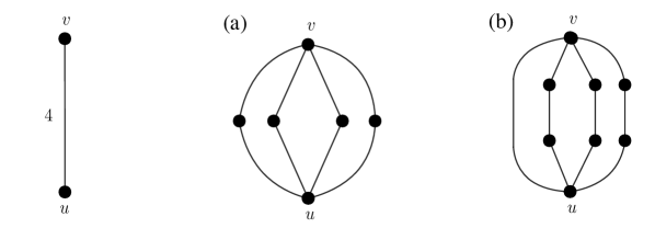
Figure 1: Two different realizations of an edge $(u,v)$ of multiplicity $4$. (a) A basic realization using paths of length $2$. (b) The spintop realization used in Section 4.

Double weights. In fact, it is convenient to generalize this further by introducing edges with double weights. A double weight of an edge $e$ is denoted $\omega\!:\!\omega^{\prime}$, where $\omega$ and $\omega^{\prime}$ are positive integers such that $\omega\leq\omega^{\prime}\leq K-1$, and its interpretation in the context of ${K\!\shortminus\!\textsf{STC}}$ is as follows: Given a spanning tree $T$,

• if $e\in E\setminus T$ then $e$ contributes $\omega$ to the congestion $\text{cng}_{G,T}(f)$ of any edge $f\in T$ for which $e\in\partial_{G,T}(f)$, and

• if $e\in T$ then $e$ contributes $\omega^{\prime}$ to its own congestion, $\text{cng}_{G,T}(e)$.

The lemma below provides a simple-graph realization of double-weighted edges. It implies that including such edges does not affect the computational complexity of ${K\!\shortminus\!\textsf{STC}}$, allowing us to formulate our proofs in terms of graphs where some edges have double weights.

Lemma 2.1.

Let $(u,v)$ be an edge in $G$ with double weight $\omega\!:\!\omega^{\prime}$, where $\omega\leq\omega^{\prime}\leq K-1$. Consider another graph $G^{\prime}$ obtained from $G$ by removing $(u,v)$, and for each $i=1,2,\cdots,\omega$ adding a new vertex $w_{i}$ with two edges: edge $(u,w_{i})$ of weight $1$ and edge $(w_{i},v)$ of weight $\omega^{\prime}-\omega+1$ (see Figure 2a for an example). Then, $\text{stc}(G)\leq K$ if and only if $\text{stc}(G^{\prime})\leq K$.

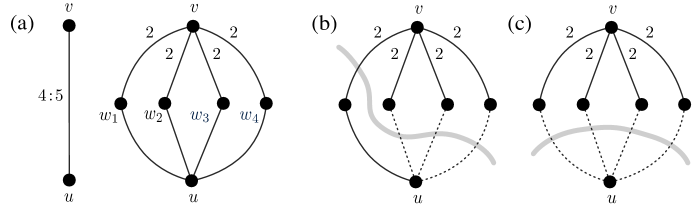
Figure 2: (a) On the left, an edge $(u,v)$ with double weight $4\!:\!5$ in $G$. On the right, the realization of $(u,v)$ in $G^{\prime}$. If one applies the spintop realization of the edges from $v$ to $w_{i}$’s, as in Figure 1b, then the subgraph on the right realizing $(u,v)$ is bipartite and all its nodes are within distance $2$ from $v$. Figures (b) and (c) illustrate the proof of Lemma 2.1: (b) the traversal of $T^{\prime}$ and the cut of $(u,v)$ when $(u,v)\in T$, (c) the traversal of $T^{\prime}$ and the cut containing $(u,v)$ when $(u,v)\notin T$. Solid lines are tree edges and dotted lines are non-tree edges.

Proof 2.2.

Denote by $W={\left\{w_{1},w_{2},...,w_{\omega}\right\}}$ the set of new vertices, and by $W_{u}={\left\{(u,w_{i})\;|\;w_{i}\in W\right\}}$ and $W_{v}={\left\{(w_{i},v)\;|\;w_{i}\in W\right\}}$ the sets of new edges added to $G^{\prime}$.

($\Rightarrow$) Suppose that $G$ has a spanning tree $T$ with $\text{cng}_{G}(T)\leq K$. We will show that there exists a spanning tree $T^{\prime}$ of $G^{\prime}$ with $\text{cng}_{G^{\prime}}(T^{\prime})\leq K$. We break the proof into two cases, in both cases showing that $\text{cng}_{G^{\prime},T^{\prime}}(e)\leq K$ for each edge $e\in T^{\prime}$.

Case 1: $(u,v)\in T$.

Consider the spanning tree $T^{\prime}=T\setminus{\left\{(u,v)\right\}}\cup W_{v}\cup{\left\{(w_{1},u)\right\}}$ of $G^{\prime}$ (see Figure 2b). For every edge $(x,y)\in E\setminus{\left\{(u,v)\right\}}$, the $x$-to-$y$ paths in $T$ and $T^{\prime}$ are the same, except that if the $x$-to-$y$ path in $T$ traverses edge $(u,v)$ then the $x$-to-$y$ path in $T^{\prime}$ traverses $(u,w_{1}),(w_{1},v)$ instead. Therefore,

• If $e\in T^{\prime}\setminus(W_{v}\cup{\left\{(u,w_{1})\right\}})$, then $\partial_{G^{\prime},T^{\prime}}(e)=\partial_{G,T}(e)$. So $\text{cng}_{G^{\prime},T^{\prime}}(e)=\text{cng}_{G,T}(e)\leq K$.

• If $e=(u,w_{1})$, then $\partial_{G^{\prime},T^{\prime}}(e)=\partial_{G,T}(u,v)\setminus{\left\{(u,v)\right\}}\cup W_{u}$. By the definition of double weights, $(u,v)$ contributes $\omega^{\prime}$ to $\text{cng}_{G,T}(u,v)$ while each edge in $W_{u}$ contributes $1$ to $\text{cng}_{G^{\prime},T^{\prime}}(e)$. Hence, $\text{cng}_{G^{\prime},T^{\prime}}(e)=\text{cng}_{G,T}(u,v)-\omega^{\prime}+\omega\leq\text{cng}_{G,T}(e)\leq K$.

• If $e=(w_{1},v)$, then $\partial_{G^{\prime},T^{\prime}}(e)=\partial_{G,T}(u,v)\setminus{\left\{(u,v)\right\}}\cup{\left\{e\right\}}\cup(W_{u}\setminus{\left\{(w_{1},u)\right\}})$. Since $e$ contributes $\omega^{\prime}-\omega+1$ to its own congestion, we have: $\text{cng}_{G^{\prime},T^{\prime}}(e)=\text{cng}_{G,T}(u,v)-\omega^{\prime}+(\omega^{\prime}-\omega+1)+(\omega-1)=\text{cng}_{G,T}(u,v)\leq K$.

• Lastly, if $e\in W_{v}\setminus{\left\{(w_{1},v)\right\}}$ then it is a leaf edge, we have $\text{cng}_{G^{\prime},T^{\prime}}(e)=\omega^{\prime}-\omega+2\leq\omega^{\prime}+1\leq K$.

Case 2: $(u,v)\notin T$.

Let $T^{\prime}=T\cup W_{v}$, which is a spanning tree of $G^{\prime}$ (see Figure 2c). We consider the following sub-cases:

• If $e\in W_{v}$ then, as $e$ is a leaf edge, we have $\text{cng}_{G^{\prime},T^{\prime}}(e)=\omega^{\prime}-\omega+2\leq\omega^{\prime}+1\leq K$.

• If $e\in T^{\prime}\setminus W_{v}$ and $e$ is not on the $u$-to-$v$ path in $T^{\prime}$, then $\partial_{G^{\prime},T^{\prime}}(e)=\partial_{G,T}(e)$. So $\text{cng}_{G^{\prime},T^{\prime}}(e)=\text{cng}_{G,T}(e)\leq K$.

• If $e\in T^{\prime}\setminus W_{v}$ and $e$ is on the $u$-to-$v$ path in $T^{\prime}$, then $\partial_{G^{\prime},T^{\prime}}(e)=\partial_{G,T}(e)\setminus{\left\{(u,v)\right\}}\cup W_{u}$. Since $(u,v)$ contributes $\omega$ to $\text{cng}_{G,T}(e)$ and $W_{u}$ also contributes $\omega$ to $\text{cng}_{G^{\prime},T^{\prime}}(e)$, we have $\partial_{G^{\prime},T^{\prime}}(e)=\partial_{G,T}(e)\leq K$.

We have shown that $\text{cng}_{G^{\prime}}(T^{\prime})\leq K$ in all cases, which completes the proof for the forward implication. We now proceed to the proof of the converse implication.

($\Leftarrow$) Let $T^{\prime}$ be the spanning tree of $G^{\prime}$ with congestion $\text{cng}_{G^{\prime}}(T^{\prime})\leq K$. We will show that there exists a spanning tree $T$ of $G$ with $\text{cng}_{G}(T)\leq K$. Note that, for any $w_{i}\in W$, $T^{\prime}$ traverses at least one of the two edges $(u,w_{i})$ and $(w_{i},v)$. Furthermore, at most one vertex in $W$ is a non-leaf. We consider three cases. In the first two cases the arguments follow the same pattern as in the proof for the $(\Rightarrow)$ implication, in essence reversing the modification of the spanning tree. Then the third case reduces to the second case.

Case 1: Exactly one vertex in $W$ is a non-leaf in $T^{\prime}$.

Without loss of generality, we can assume $w_{1}$ is a non-leaf vertex (that is, both $(u,w_{1})$ and $(w_{1},v)$ are in $T$) and $W\setminus{\left\{w_{1}\right\}}$ are leaves. We construct $T$ by adding $(u,v)$ to $T^{\prime}$ and removing all vertices of $W$ and their incident edges from $T$. By the construction, $T$ is a spanning tree of $G$. We have:

• If $e\in T\setminus{\left\{(u,v)\right\}}$, then $\text{cng}_{G,T}(e)=\text{cng}_{G^{\prime},T^{\prime}}(e)\leq K$.

• If $e=(u,v)$, then $\text{cng}_{G,T}(e)\leq\text{cng}_{G^{\prime},T^{\prime}}(v,w_{1})\leq K$.

Case 2: All vertices in $W$ are leaves and $T^{\prime}$ traverse all edges in $W_{v}$.

Let $T=T^{\prime}\setminus W_{v}$, which is a spanning tree of $G$. Then

• If $e\in T$ and $e$ is not on the $u$-to-$v$ path in $T$, then $\text{cng}_{G,T}(e)=\text{cng}_{G^{\prime},T^{\prime}}(e)\leq K$.

• If $e\in T$ and $e$ is on the $u$-to-$v$ path in $T$, then $(u,v)$ and $W_{u}$ contribute the same amount $\omega$ to the congestion of $e$ in $T$ and $T^{\prime}$, respectively, implying that $\text{cng}_{G,T}(e)=\text{cng}_{G^{\prime},T^{\prime}}(e)\leq K$.

Case 3: All vertices in $W$ are leaves and $T^{\prime}$ traverses at least one edge in $W_{u}$.

In this case, we consider another spanning tree $T^{\prime\prime}$ of $G^{\prime}$ that traverses all edges in $W_{v}$ and does not use any edge in $W_{u}$. It is sufficient to show that $\text{cng}_{G^{\prime}}(T^{\prime\prime})\leq\text{cng}_{G^{\prime}}(T^{\prime})$, since it implies that $\text{cng}_{G^{\prime}}(T^{\prime\prime})\leq K$, and then we can apply Case 2 to $T^{\prime\prime}$. We examine the congestion values of each edge $e\in T^{\prime\prime}$:

• If $e\in T^{\prime\prime}\setminus W_{v}$ and $e$ is not on the $u$-to-$v$ path in $T^{\prime\prime}$, then $e\in T^{\prime}$ and $\partial_{G^{\prime},T^{\prime\prime}}(e)=\partial_{G^{\prime},T^{\prime}}(e)$, implying $\text{cng}_{G^{\prime},T^{\prime\prime}}(e)=\text{cng}_{G^{\prime},T^{\prime}}(e)$.

• If $e\in T^{\prime\prime}\setminus W_{v}$ and $e$ is on the $u$-to-$v$ path in $T^{\prime\prime}$, then for each vertex $w_{i}\in W$ either $(u,w_{i})$ contributes $1$ or $(w_{i},v)$ contributes $\omega^{\prime}-\omega+1\geq 1$ to $\text{cng}_{G^{\prime},T^{\prime}}(e)$. On the other hand, in $T^{\prime\prime}$, all edges in $W_{u}$ are in $\partial_{G^{\prime},T^{\prime\prime}}(e)$ and contribute a total of $\omega$ to $\text{cng}_{G^{\prime},T^{\prime\prime}}(e)$. Thus, $\text{cng}_{G^{\prime},T^{\prime\prime}}(e)\leq\text{cng}_{G^{\prime},T^{\prime}}(e)$.

• If $e\in W_{v}$, then $\text{cng}_{G^{\prime},T^{\prime\prime}}(e)=\omega^{\prime}-\omega+2\leq\omega^{\prime}+1\leq K$.

In all cases, we have proved that there is a spanning tree $T$ of $G$ that has congestion at most $K$ establishing the validity of the backward implication.

As explained earlier, in Section 4 we will use the spintop realization for weighted edges. With this, the realization of an edge $e=(u,v)$ with double weight $\omega\!:\!\omega^{\prime}$ will use the spintop realization for the edges of weight $\omega^{\prime}-\omega+1$ between $v$ and the $w_{i}$’s. The property of this realization that will be crucial in Section 4 is that it is bipartite and all its nodes are within distance $2$ from $v$.

Remark: Some readers may have noticed that there is a simpler way to realize an edge $(u,v)$ with a double weight $\omega\!:\!\omega^{\prime}$: replace it by a length-$2$ path $(u,w)$, $(w,v)$, where $w$ is a new vertex, edge $(u,w)$ has weight $\omega$, and edge $(w,v)$ has weight $\omega^{\prime}$. This indeed works, but can be used only when $\omega+\omega^{\prime}\leq K$. This is because, in this construction, if $w$ is a leaf of a spanning tree, the congestion of the tree edge from $w$ will be $\omega+\omega^{\prime}$, and this congestion value cannot exceed $K$. This realization of double-weighted edges would suffice for our proof in Section 3, but not the one in Section 4. (It may also be useful for establishing other hardness results for STC.)

3 ${\mathbb{NP}}$-completeness proof of ${K\!\shortminus\!\textsf{STC}}$ for $K\geq 5$

In this section we prove our main result, the ${\mathbb{NP}}$-completeness of ${K\!\shortminus\!\textsf{STC}}$. Our proof uses an ${\mathbb{NP}}$-complete variant of the satisfiability problem called (2P1N)-SAT [7, 25]. An instance of (2P1N)-SAT is a boolean expression $\phi$ in conjunctive normal form, where each variable occurs exactly three times, twice positively and once negatively, and each clause contains exactly two or three literals of different variables. The objective is to decide if $\phi$ is satisfiable, that is if there is a satisfying assignment that makes $\phi$ true.

For each constant $K$, ${K\!\shortminus\!\textsf{STC}}$ is clearly in ${\mathbb{NP}}$. We will present a polynomial-time reduction from (2P1N)-SAT. In this reduction, given an instance $\phi$ of (2P1N)-SAT, we construct a graph $G$ with the following property:

$(\ast)$ $\phi$ has a satisfying truth assignment if and only if $\text{stc}(G)\leq K$.

Throughout the proof, the three literals of $x_{i}$ in $\phi$ will be denoted by $x_{i}$, $x^{\prime}_{i}$, and ${\bar{x}}_{i}$, where $x_{i}$, $x^{\prime}_{i}$ are the two positive occurrences of $x_{i}$ and ${\bar{x}}_{i}$ is the negative occurrence of $x_{i}$. We will also use notation ${\tilde{x}}_{i}$ to refer to an unspecified literal of $x_{i}$, that is ${\tilde{x}}_{i}\in{\left\{x_{i},x^{\prime}_{i},{\bar{x}}_{i}\right\}}$.

We now describe the reduction. Set $k_{i}=K-i$ for $i=1,2,3,4$. (In particular, for $K=5$, we have $k_{1}=4$, $k_{2}=3$, $k_{3}=2$, $k_{4}=1$). $G$ will consist of gadgets corresponding to variables, with the gadget corresponding to $x_{i}$ having three vertices $x_{i}$, $x^{\prime}_{i}$, and ${\bar{x}}_{i}$, that represent its three occurrences in the clauses. $G$ will also have vertices representing clauses and edges connecting literals with the clauses where they occur (see Figure 3b for an example). As explained in Section 2, without any loss of generality we can allow edges in $G$ to have constant-valued weights, single or double. Specifically, starting with $G$ empty, the construction of $G$ proceeds as follows:

• Add a root vertex $r$.

• For each variable $x_{i}$, construct the $x_{i}$-gadget (see Figure 3a). This gadget has three vertices corresponding to the literals: a negative literal vertex ${\bar{x}}_{i}$ and two positive literal vertices $x_{i},x_{i}^{\prime}$, and two auxiliary vertices $y_{i}$ and $z_{i}$. Its edges and their weights are given in the table below:

  edge	$({\bar{x}}_{i},z_{i})$	$(z_{i},x_{i})$	$(x_{i},x_{i}^{\prime})$	$(r,x_{i}^{\prime})$	$(r,y_{i})$	$(y_{i},z_{i})$	$(y_{i},\bar{x}_{i})$
  weight	$1\!:\!k_{3}$	$1\!:\!k_{3}$	$1\!:\!k_{2}$	$k_{3}$	$k_{4}$	$k_{4}$	$1\!:\!k_{2}$

• For each clause $c$, create a clause vertex $c$. For each literal ${\tilde{x}}_{i}$ in $c$, add the corresponding clause-to-literal edge $(c,{\tilde{x}}_{i})$ of weight $1\!:\!k_{2}$. Importantly, as all literals in $c$ correspond to different variables, these edges will go to different variable gadgets.

• For each two-literal clause $c$, add a root-to-clause edge $(r,c)$ of weight $1\!:\!k_{1}$.

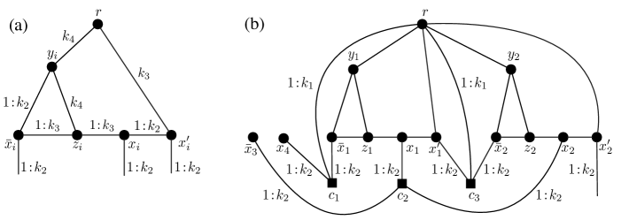
Figure 3: (a)The $x_{i}$-gadget. (b) An example of a partial graph $G$ for the boolean expression $\phi=c_{1}\land c_{2}\land c_{3}\land\cdots$ where $c_{1}={\bar{x}}_{1}\lor x_{4}$, $c_{2}=x_{1}\lor x_{2}\lor{\bar{x}}_{3}$, and $c_{3}=x_{1}\lor{\bar{x}}_{2}$. (The weights of edges inside the variable gadgets are not shown.)

We now show that $G$ has the required property $(\ast)$, proving the two implications separately.

$(\Rightarrow)$ Suppose that $\phi$ has a satisfying assignment. Using this assignment, we construct a spanning tree $T$ of $G$ as follows:

• For every $x_{i}$-gadget, include in $T$ edges $(r,x_{i}^{\prime})$, $(r,y_{i})$, and $(y_{i},z_{i})$. If $x_{i}=0$, include in $T$ edges $(\bar{x}_{i},z_{i})$ and $(x_{i},x_{i}^{\prime})$, otherwise include in $T$ edges $(y_{i},\bar{x}_{i})$ and $(z_{i},x_{i})$.

• For each clause $c$, include in $T$ one clause-to-literal edge that is incident to any literal vertex that satisfies $c$ in our chosen truth assignment for $\phi$.

By routine inspection, $T$ is indeed a spanning tree of $G$: Each $x_{i}$-gadget is traversed from $r$ without cycles, and all clause vertices are leaves of $T$. Figures 4 and 5 show how $T$ traverses an $x_{i}$-gadget in different cases, depending on whether $x_{i}=0$ or $x_{i}=1$ in the truth assignment for $\phi$, and on which literals are chosen to satisfy each clause. Note that the edges with double weights satisfy the assumption of Lemma 2.1 in Section 2, that is each such weight $1\!:\!\omega^{\prime}$ satisfies $1\leq\omega^{\prime}\leq K-1$.

We need to verify that each edge in $T$ has congestion at most $K$. All the clause vertices are leaves in $T$, thus the congestion of each clause-to-literal edge is $k_{2}+2=K$ (this holds for both three-literal and two-literal clauses). To analyze the congestion of the edges inside an $x_{i}$-gadget, we consider two cases, depending on the value of $x_{i}$ in our truth assignment.

When $x_{i}=0$, we have two sub-cases (a) and (b) as shown in Figure 4. The congestions of the edges in the $x_{i}$-gadget are as follows:

• In both cases, $\text{cng}_{G,T}(r,x_{i}^{\prime})=k_{3}+3$.

• In case (a), $\text{cng}_{G,T}(r,y_{i})=k_{4}+3$. In case (b), it is $k_{4}+2$.

• In case (a), $\text{cng}_{G,T}(y_{i},z_{i})=k_{4}+4$. In case (b), it is $k_{4}+3$.

• In case (a), $\text{cng}_{G,T}({\bar{x}}_{i},z_{i})=k_{3}+3$. In case (b), it is $k_{3}+2$.

• In both cases, $\text{cng}_{G,T}(x_{i},x_{i}^{\prime})=k_{2}+2$.

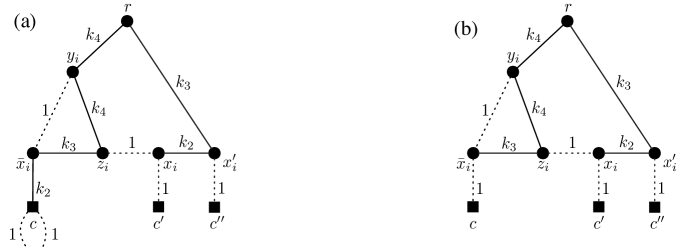
Figure 4: The traversal of the $x_{i}$-gadget by $T$ when $x_{i}=0$. Solid lines are tree edges, dotted lines are non-tree edges. (a) ${\bar{x}}_{i}$ is chosen by clause $c$. (b) ${\bar{x}}_{i}$ is not chosen by clause $c$.

On the other hand, when $x_{i}=1$, we have four sub-cases. Figure 4 illustrates cases (a)–(c). In case (d) (not shown in Figure 4), none of the positive literal vertices $x_{i},x_{i}^{\prime}$ is chosen to satisfy their corresponding clauses. The congestions of the edges in the $x_{i}$-gadget are as follows:

• In cases (a) and (b), $\text{cng}_{G,T}(r,x_{i}^{\prime})=k_{3}+3$. In cases (c) and (d), it is $k_{3}+2$.

• In cases (a) and (c), $\text{cng}_{G,T}(r,y_{i})=k_{4}+4$. In cases (b) and (d), it is $k_{4}+3$.

• In cases (a) and (c), $\text{cng}_{G,T}(y_{i},z_{i})=k_{4}+4$. In cases (b) and (d), it is $k_{4}+3$.

• In cases (a) and (c), $\text{cng}_{G,T}(z_{i},x_{i})=k_{3}+3$. In cases (b) and (d), it is $k_{3}+2$.

• In all cases, $\text{cng}_{G,T}(y_{i},{\bar{x}}_{i})=k_{2}+2$.

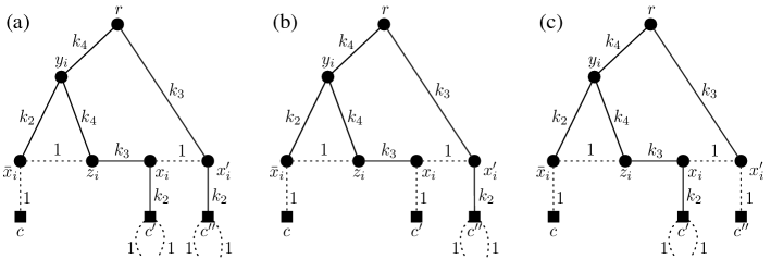
Figure 5: The traversal of the $x_{i}$-gadget by $T$ when $x_{i}=1$. By $c$, $c^{\prime}$ and $c^{\prime\prime}$ we denote the clauses that contain literals ${\bar{x}}_{i}$, $x_{i}$ and $x^{\prime}_{i}$, respectively. (a) $x_{i}$ and $x^{\prime}_{i}$ are chosen by clauses $c^{\prime}$ and $c^{\prime\prime}$. (b) $x^{\prime}_{i}$ is chosen by clause $c^{\prime\prime}$. (c) $x_{i}$ is chosen by clause $c^{\prime}$.

In summary, the congestion of each edge of $T$ is at most $K$. Thus $\text{cng}_{G}(T)\leq K$; in turn, $\text{stc}(G)\leq K$, as claimed.

$(\Leftarrow)$ We now prove the other implication in $(\ast)$. We assume that $G$ has a spanning tree $T$ with $\text{cng}_{G}(T)\leq K$. We will show how to convert $T$ into a satisfying truth assignment for $\phi$. The proof consists of a sequence of claims showing that $T$ must have a special form that will allow us to define this truth assignment.

Claim 1.

Each $x_{i}$-gadget satisfies the following property: for each literal vertex ${\tilde{x}}_{i}$, if some edge $e$ of $T$ (not necessarily in the $x_{i}$-gadget) is on the $r$-to-${\tilde{x}}_{i}$ path in $T$, then $\partial_{G,T}(e)$ contains at least two distinct edges from this gadget other than $(y_{i},z_{i})$.

This claim is straightforward: it follows directly from the fact that there are two edge-disjoint paths from $r$ to any literal vertex ${\tilde{x}}_{i}\in{\left\{{\bar{x}}_{i},x_{i},x_{i}^{\prime}\right\}}$ that do not use edge $(y_{i},z_{i})$.

Claim 2.

For each two-literal clause $c$, edge $(r,c)$ is not in $T$.

For each literal ${\tilde{x}}_{i}$ of clause $c$, there is an $r$-to-$c$ path via the $x_{i}$-gadget, so, together with edge $(r,c)$, $G$ has three disjoint $r$-to-$c$ paths. Thus, if $(r,c)$ were in $T$, its congestion would be at least $k_{1}+2>K$, proving Claim 2.

Claim 3.

All clause vertices are leaves in $T$.

To prove Claim 3, suppose there is a clause $c$ that is not a leaf. Then, by Claim 2, $c$ has at least two clause-to-literal edges in $T$, say $(c,{\tilde{x}}_{i})$ and $(c,{\tilde{x}}_{j})$. We can assume that the last edge on the $r$-to-$c$ path in $T$ is $e=(c,{\tilde{x}}_{i})$. Clearly, $r\in T_{{\tilde{x}}_{i},c}$ and ${\tilde{x}}_{j}\in T_{c,{\tilde{x}}_{i}}$. By Claim 1, at least two edges of the $x_{j}$-gadget are in $\partial_{G,T}(e)$, and they contribute at least $2$ to $\text{cng}_{G,T}(e)$. We now have some cases to consider.

If $c$ is a two-literal clause, its root-to-clause edge $(r,c)$ is also in $\partial_{G,T}(e)$, by Claim 2. Thus, $\text{cng}_{G,T}(e)\geq k_{2}+3>K$ (see Figure 6a). So assume now that $c$ is a three-literal clause, and let ${\tilde{x}}_{l}\neq{\tilde{x}}_{i},{\tilde{x}}_{j}$ be the third literal of $c$. If $T$ contains $(c,{\tilde{x}}_{l})$, the $x_{l}$-gadget would also contribute at least $2$ to $\text{cng}_{G,T}(e)$, so $\text{cng}_{G,T}(e)\geq k_{2}+4>K$ (see Figure 6b). Otherwise, $(c,{\tilde{x}}_{l})\notin T$, and $(c,{\tilde{x}}_{l})$ itself contributes $1$ to $\text{cng}_{G,T}(e)$, so $\text{cng}_{G,T}(e)\geq k_{2}+3>K$ (see Figure 6c).

We have shown that if a clause vertex $c$ is not a leaf in $T$, then in all cases the congestion of $T$ would exceed $K$, completing the proof of Claim 3.

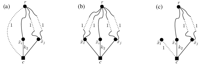
Figure 6: Illustration of the proof of Claim 3. In (a) $c$ is a two-literal clause; in (b) and (c), $c$ is a three-literal clause.

Claim 4.

For each $x_{i}$-gadget, edge $(r,x_{i}^{\prime})$ is in $T$.

Towards contradiction, suppose that $(r,x_{i}^{\prime})$ is not in $T$. Let $(x_{i}^{\prime},c)$ be the clause-to-literal edge of $x_{i}^{\prime}$. If only one of the two edges $(x_{i}^{\prime},x_{i}),(x_{i}^{\prime},c)$ is in $T$, making $x^{\prime}_{i}$ a leaf, then the congestion of that edge is $k_{3}+k_{2}+1>K$. Otherwise, both $(x_{i}^{\prime},x_{i}),(x_{i}^{\prime},c)$ are in $T$. Because $c$ is a leaf in $T$ by Claim 3, $e=(x_{i},x_{i}^{\prime})$ is the last edge on the $r$-to-$x_{i}^{\prime}$ path in $T$. As shown in Figure 7a, $\text{cng}_{G,T}(e)\geq k_{3}+k_{2}+2>K$. This proves Claim 4.

Claim 5.

For each $x_{i}$-gadget, edge $(r,y_{i})$ is in $T$.

To prove this claim, suppose $(r,y_{i})$ is not in $T$. We consider the congestion of the first edge $e$ on the $r$-to-$y_{i}$ path in $T$. By Claims 3 and 4, we have $e=(r,x_{i}^{\prime})$, all vertices of the $x_{i}$-gadget have to be in $T_{x_{i}^{\prime},r}$, and $T_{x_{i}^{\prime},r}$ does not contain literal vertices of another variable $x_{j}\neq x_{i}$. For each literal ${\tilde{x}}_{i}$ of $x_{i}$, if a clause-to-literal edge $(c,{\tilde{x}}_{i})$ is in $T$, then the two other edges of $c$ contribute $2$ to $\text{cng}_{G,T}(e)$, otherwise $(c,{\tilde{x}}_{i})$ contributes $1$ to $\text{cng}_{G,T}(e)$. Then, $\text{cng}_{G,T}(e)\geq k_{4}+k_{3}+3>K$ (see Figure 7b), proving Claim 5.

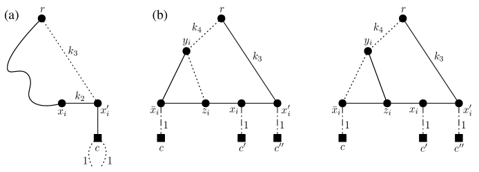
Figure 7: (a) Illustration of the proof of Claim 4. (b) Illustration of the proof of Claim 5. Dot-dashed lines are edges that may or may not be in $T$.

Claim 6.

For each $x_{i}$-gadget, exactly one of edges $(z_{i},x_{i})$ and $(x_{i},x_{i}^{\prime})$ is in $T$.

By Claims 4 and 5, edges $(r,y_{i})$ and $(r,x_{i}^{\prime})$ are in $T$. Since the clause neighbor $c^{\prime}$ of $x_{i}$ is a leaf of $T$, by Claim 3, if none of $(z_{i},x_{i})$, $(x_{i},x_{i}^{\prime})$ were in $T$, $x_{i}$ would not be reachable from $r$ in $T$. Thus, at least one of them is in $T$. Now, assume both $(z_{i},x_{i})$ and $(x_{i},x_{i}^{\prime})$ are in $T$ (see Figure 8a). Then, edge $(y_{i},z_{i})$ is not in $T$, as otherwise we would create a cycle. Let us consider the congestion of edge $e=(r,x_{i}^{\prime})$. Clearly, $x_{i}$ and $x_{i}^{\prime}$ are in $T_{x_{i}^{\prime},r}$. The edges of the two clause neighbors $c^{\prime}$ and $c^{\prime\prime}$ of $x_{i}$ and $x_{i}^{\prime}$ contribute at least $2$ to $\text{cng}_{G,T}(e)$, by Claim 3. In addition, by Claim 1, besides $e$ and $(y_{i},z_{i})$, $\partial_{G,T}(e)$ contains another edge of the $x_{i}$-gadget which contributes at least another $1$ to $\text{cng}_{G,T}(e)$. Thus, $\text{cng}_{G,T}(e)\geq k_{4}+k_{3}+3>K$ — a contradiction. This proves Claim 6.

Claim 7.

For each $x_{i}$-gadget, edge $(y_{i},z_{i})$ is in $T$.

By Claims 4 and 5, the two edges $(r,x_{i}^{\prime})$ and $(r,y_{i})$ are in $T$. Now assume, towards contradiction, that $(y_{i},z_{i})$ is not in $T$ (see Figure 8b). By Claim 6, only one of $(z_{i},x_{i})$ and $(x_{i},x_{i}^{\prime})$ is in $T$. Furthermore, the clause neighbor $c^{\prime}$ of $x_{i}$ is a leaf of $T$, by Claim 3. As a result, $(z_{i},x_{i})$ cannot be on the $y_{i}$-to-$z_{i}$ path in $T$. To reach $z_{i}$ from $y_{i}$, the two edges $(y_{i},{\bar{x}}_{i}),({\bar{x}}_{i},z_{i})$ have to be in $T$. Let us consider the congestion of $e=(y_{i},{\bar{x}}_{i})$. The edges of the clause neighbor $c$ of ${\bar{x}}_{i}$ contribute at least $1$ to the congestion of $e$, by Claim 3. Also, by Claim 1, besides $e$ and $(y_{i},z_{i})$, $\partial_{G,T}(e)$ contains another edge of the $x_{i}$-gadget which contributes at least $1$ to $\text{cng}_{G,T}(e)$. In total, $\text{cng}_{G,T}(e)\geq k_{4}+k_{2}+2>K$, reaching a contradiction and completing the proof of Claim 7.

Figure 8: (a) Illustration of the proof of Claim 6. (b) Illustration of the proof of Claim 7.

Claim 8.

For each $x_{i}$-gadget, if its clause-to-literal edge $({\bar{x}}_{i},c)$ is in $T$, then its other two clause-to-literal edges $(x_{i},c^{\prime})$ and $(x_{i}^{\prime},c^{\prime\prime})$ are not in $T$.

Assume the clause-to-literal edge $({\bar{x}}_{i},c)$ of the $x_{i}$-gadget is in $T$. By Claim 7, edge $(y_{i},z_{i})$ is in $T$. If $(y_{i},{\bar{x}}_{i})$ is also in $T$, edge $({\bar{x}}_{i},z_{i})$ cannot be in $T$, and it contributes $1$ to $\text{cng}_{G,T}(y_{i},{\bar{x}}_{i})$. As shown in Figure 9a, $\text{cng}_{G,T}(y_{i},{\bar{x}}_{i})=k_{2}+3>K$. Thus, $(y_{i},{\bar{x}}_{i})$ cannot be in $T$. Since $c$ is a leaf of $T$, edge $({\bar{x}}_{i},z_{i})$ has to be in $T$, for otherwise ${\bar{x}}_{i}$ would not be reachable from $r$. By Claim 6, one of edges $(z_{i},x_{i})$ and $(x_{i},x_{i}^{\prime})$ is in $T$. If $(z_{i},x_{i})$ is in $T$ (see Figure 9b), $\text{cng}_{G,T}(y_{i},z_{i})\geq k_{4}+5>K$. Hence, $(z_{i},x_{i})$ is not in $T$, which implies that $(x_{i},x_{i}^{\prime})$ is in $T$.

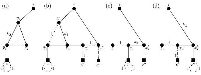
Figure 9: Illustration of the proof of Claim 8.

Now, we proceed by contradiction assuming that at least one other clause-to-literal edge of the $x_{i}$-gadget is in $T$. If edge $(x_{i},c^{\prime})$ is in $T$, $\text{cng}_{G,T}(x_{i},x_{i}^{\prime})\geq k_{2}+3>K$, as shown in Figure 9c. Similarly, if $(x_{i}^{\prime},c^{\prime\prime})$ is in $T$, $\text{cng}_{G,T}(r,x_{i}^{\prime})\geq k_{3}+4>K$ (see Figure 9d). So we reach a contradiction in both cases, thus proving Claim 8.

We are now ready to complete the proof of the $(\Leftarrow)$ implication in the equivalence $(\ast)$. We use our spanning tree $T$ of congestion at most $K$ to create a truth assignment for $\phi$ by setting $x_{i}=0$ if the clause-to-literal edge of ${\bar{x}}_{i}$ is in $T$, otherwise $x_{i}=1$. By Claim 8, this truth assignment is well-defined. Each clause has one clause-to-literal edge in $T$ which ensures that all clauses are indeed satisfied.

4 ${\mathbb{NP}}$-completeness proof of ${K\!\shortminus\!\textsf{STC}}$ for bipartite graphs of radius $2$ and $K\geq 6$

In this section we establish the following result:

Theorem 4.1.

For any fixed integer $K\geq 6$, ${K\!\shortminus\!\textsf{STC}}$ is ${\mathbb{NP}}$-complete for bipartite graphs of radius $2$, even if they have only one vertex of degree greater than $\max(6,K-2)$.

First, we introduce a restricted variant of the satisfiability problem, which we name (M2P1N)-SAT, that is used in the reduction. An instance of (M2P1N)-SAT is a boolean expression in conjunctive normal form with the following properties:

• Each clause either contains three positive literals (a 3P-clause), or two positive literals (a 2P-clause), or two negative literals (a 2N-clause). Also, literals in the same clause are of different variables.

• Each variable appears exactly three times: once in a 3P-clause, once in a 2P-clause and once in a 2N-clause.

• Two clauses share at most one variable.

Lemma 4.2.

(M2P1N)-SAT is ${\mathbb{NP}}$-complete.

Proof 4.3.

It is clear that (M2P1N)-SAT belongs to ${\mathbb{NP}}$. To demonstrate ${\mathbb{NP}}$-completeness, we show a polynomial-time reduction from the ${\mathbb{NP}}$-complete problem called BALANCED-3SAT [14]. BALANCED-3SAT is a restriction of the satisfiability problem to boolean expressions in conjunctive normal form where, for each variable $x$, the positive literal $x$ appears the same number of times as the negative literal ${\bar{x}}$. We can further assume that every variable appears at least four times, and that, for each clause, all variables that appear in this clause are different.

Given an instance $\psi$ of BALANCED-3SAT, we construct an instance $\phi$ of (M2P1N)-SAT as follows:

• For each variable $x$ in $\psi$, if $x$ appears $2t$ times (for some integer $t\geq 2$), create $2t$ new variables $x_{0},x_{1},\ldots,x_{2t-1}$.

• Replace the $t$ positive occurrences of $x$ by even-indexed variables $x_{0},x_{2},\ldots,x_{2t-2}$, and replace its $t$ negative occurrences by odd-indexed variables $x_{1},x_{3},\ldots,x_{2t-1}$.

• Add $t$ clauses of the form $(x_{i}\lor x_{i+1})$ for $i=0,2,\ldots,2t-2$, and $t$ clauses of the form $({\bar{x}}_{i}\lor{\bar{x}}_{(i+1)\!\!\mod 2t})$ for $i=1,3,\ldots,2t-1$.

By the construction, $\phi$ is a correct instance of (M2P1N)-SAT. For each variable $x$ of $\psi$, its corresponding “cycle” of the newly added two-literal clauses in $\phi$ ensures that $x_{0}={\bar{x}}_{1}=x_{2}={\bar{x}}_{3}=\ldots=x_{2t-2}={\bar{x}}_{2t-1}$. Thus, a truth assignment that satisfies $\psi$ can be converted into a truth assignment that satisfies $\phi$ by setting the even-indexed variables to the truth value of the original variable in $\psi$, and the odd-indexed variables to the opposite value. Conversely, a truth assignment that satisfies $\phi$ can be converted into a truth assignment that satisfies $\psi$ by reversing this process. This shows that $\psi$ is satisfiable if and only if $\phi$ is satisfiable, completing the proof of the lemma.

In order to prove Theorem 4.1, we show a polynomial-time reduction from (M2P1N)-SAT. Given an instance $\phi$ of (M2P1N)-SAT, we construct a graph $G$ such that

$(\ast)$ $\phi$ has a satisfying truth assignment if and only if $\text{stc}(G)\leq K$.

Graph $G$ will be bipartite, of radius $2$, and will have only one vertex of degree larger than $\max(6,K-2)$. We will describe $G$ using some double-weighted edges, that we refer to as fat edges. As previously discussed in Section 2, here we need a specific realization of these double weighted edges, in which weights are realized using the spintop graph. (See Figures 1 and 2.) For $i\in{\left\{1,2,3,4,5\right\}}$, let $k_{i}=K-i$. We start with an empty graph $G$ and proceed as follows:

• Add a root vertex $r$.

• For each variable $x$ of $\phi$, add a variable vertex $x$ and a root-to-vertex edge $(r,x)$.

• For each clause $c$, add a clause vertex $c$, and add edges from $c$ to the vertices representing variables whose literals (positive or negative) appear in $c$. If clause $c$ contains all positive literals, we call its clause-to-variable edges positive-clause edges, otherwise its clause-to-variable edges are negative-clause edges.

• For each 2P-clause vertex $c$, add a fat edge $(r,c)$ of double weight $k_{5}\!:\!k_{1}$.

• For each 2N-clause vertex $c$, add a fat edge $(r,c)$ of double weight $k_{4}\!:\!k_{1}$.

See Figure 10a for an example of a partial graph constructed using the above rules. By routine inspection, taking into account that the weighted edges use the spintop realization, $G$ is bipartite, all vertices are at distance at most $2$ from $r$, and $r$ is the only vertex of degree larger than $\max(6,K-2)$. We now proceed to show that $G$ satisfies property $(\ast)$.

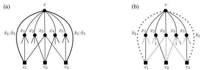
Figure 10: (a) An example of a partial graph $G$ for $\phi=c_{1}\land c_{2}\land c_{3}\land\cdots$ where $c_{1}=(\bar{x}_{1}\lor\bar{x}_{3}),c_{2}=(x_{2}\lor x_{3}\lor x_{4}),c_{3}=(x_{3}\lor x_{5})$. Bold lines represent fat edges with given double weights. (b) An example of a partial tree $T$ of $G$ where $x_{1}$ is chosen by $c_{1}$, $x_{2}$ by $c_{2}$, $x_{5}$ is by $c_{3}$. Solid lines are tree edges, dotted lines are non-tree edges, and dot-dashed lines are edges that may or may not be in $T$. Non-tree double-weighted edges contribute the indicated weights to edge congestion.

$(\Rightarrow)$ Assume that $\phi$ has a satisfying truth assignment. From this assignment we construct a spanning tree $T$ of $G$ by adding all root-to-vertex edges, and, for each clause $c$, adding to $T$ an edge from $c$ to any variable vertex whose literal satisfies $c$ (see Figure 10b). By the construction, $T$ is a spanning tree of $G$. Note that all clause vertices in $T$ are leaves and all fat edges are non-tree edges.

Now, we proceed to verify that all tree edges of $T$ have congestion at most $K$. We start with leaf edges of $T$. The congestion of the leaf edge of a 3P-clause is $3$. For a 2P-clause, the congestion of its leaf edge is $K-3$, because its fat edge contributes $k_{5}=K-5$. For a 2N-clause, the congestion of its leaf edge is $K-2$, because its fat edge contributes $k_{4}=K-4$.

Next, consider the root-to-vertex edge of a variable $x_{i}$. If $x_{i}$ is not chosen to satisfy any clauses, then $\text{cng}_{G,T}(r,x_{i})=4$ (see Figure 11a). If it is chosen to satisfy only its 3P-clause, then $\text{cng}_{G,T}(r,x_{i})=5$ (see Figure 11b). If it is chosen to satisfy only its 2P-clause, then $\text{cng}_{G,T}(r,x_{i})=k_{5}+4=K-1$ (see Figure 11c). If it is chosen to satisfy both its 3P-clause and its 2P-clause, then $\text{cng}_{G,T}(r,x_{i})=k_{5}+5=K$ (see Figure 11d). Finally, if it is chosen to satisfy its 2N-clause, then $\text{cng}_{G,T}(r,x_{i})=k_{4}+4=K$ (see Figure 11e).

There are also edges inside the realizations of fat edges, but their congestion does not exceed $K$, by Lemma 2.1. We have thus shown that the congestions of all edges in $T$ are at most $K$; that is, $\text{stc}(G)\leq K$.

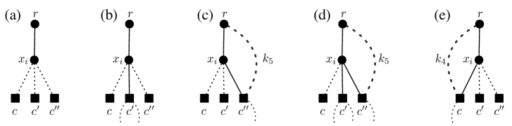
Figure 11: By $c,c^{\prime},c^{\prime\prime}$, we denote the 2N-clause, 3P-clause and 2P-clause of $x_{i}$ respectively. In (a), $x_{i}$ is not chosen by any clause, it is chosen by $c^{\prime}$ in (b), by $c^{\prime\prime}$ in (c), by both $c^{\prime}$ and $c^{\prime\prime}$ in (d), and by $c$ in (e).

$(\Leftarrow)$ Assume $T$ is a spanning tree of $G$ with $\text{cng}_{G}(T)\leq K$. From $T$, we will construct a satisfying truth assignment for $\phi$. The argument here, while much shorter, has a subtle aspect that was not present in the proof in Section 3, namely now it is not necessarily true that all clause vertices in $T$ are leaves. (It’s not hard to see that for large $K$ a single branch out of $r$ may visit multiple variables via their 3P-clause vertices.)

We present two claims showing that $T$ must have a special form that will allow us to define the truth assignment for $\phi$.

Claim 9.

For each two-literal clause $c$, its fat edge $(r,c)$ is not in $T$.

For each literal of $c$, there is an $r$-to-$c$ path via the variable vertex of this literal. So, together with edge $(r,c)$, $G$ has three disjoint $r$-to-$c$ paths. Thus, if $(r,c)$ were in $T$, its congestion would be at least $k_{1}+2>K$, proving Claim 9.

Claim 10.

For each variable vertex $x_{i}$, if its negative-clause edge is in $T$ then its two positive-clause edges are not in $T$.

Denote by $c,c^{\prime},c^{\prime\prime}$ the 2N, 3P, 2P-clause vertices of $x_{i}$ respectively. Since $c,c^{\prime},c^{\prime\prime}$ all contain variable $x_{i}$, they cannot share any other variables (by the definition of (M2P1N)-SAT). Therefore, the four literals in $c,c^{\prime},c^{\prime\prime}$ other than $x_{i}$ and ${\bar{x}}_{i}$ must all involve different variables.

Toward contradiction, suppose $(x_{i},c)$ and at least one of $(x_{i},c^{\prime}),(x_{i},c^{\prime\prime})$ are in $T$. We will estimate the congestion of the first edge $e=(r,v)$ on the $r$-to-$c$ path in $T$.

By Claim 9, fat edge $(r,c)$ contributes $k_{4}$ to $\text{cng}_{G,T}(e)$. The rest of the argument is based on the following two observations: (i) If a clause ${\tilde{c}}\in{\left\{c,c^{\prime},c^{\prime\prime}\right\}}$ is in $T_{v,r}$, and some variable $x$ is in ${\tilde{c}}$, then either $(r,x)$ or $(x,{\tilde{c}})$ is in $\partial_{G,T}(e)$; that is, this $x$ contributes $1$ to $\text{cng}_{G,T}(e)$. (This is true whether or not $v=x$. And if $x=x_{i}$ and ${\tilde{c}}=c$, then $(r,x_{i})$ is the edge that contributes to $\text{cng}_{G,T}(e)$.) On the other hand, (ii) if a clause ${\tilde{c}}\in{\left\{c^{\prime},c^{\prime\prime}\right\}}$ is not in $T_{v,r}$, then $(x_{i},{\tilde{c}})$ contributes $1$ to $\text{cng}_{G,T}(e)$.

Now we have some cases to consider. First, if $c^{\prime}\in T_{v,r}$ and $c^{\prime\prime}\notin T_{v,r}$, by the above observations, four different variables in $c,c^{\prime}$ contribute $4$ to $\text{cng}_{G,T}(e)$ and $(x_{i},c^{\prime\prime})$ contributes $1$. In total, $\text{cng}_{G,T}(e)\geq k_{4}+4+1>K$. On the other hand, when $c^{\prime\prime}\in T_{v,r}$ and $c^{\prime}\notin T_{v,r}$, the three different variables of $c,c^{\prime\prime}$ contribute $3$ while $(x_{i},c^{\prime})$ contributes $1$ to $\text{cng}_{G,T}(e)$. Also, the fat edge $(r,c^{\prime\prime})$ contributes $k_{5}$, by Claim 9. Thus, $\text{cng}_{G,T}(e)\geq k_{4}+k_{5}+3+1>K$. Lastly, when both $c^{\prime},c^{\prime\prime}$ are in $T_{v,r}$, the five different variables of $c,c^{\prime},c^{\prime\prime}$ contribute to $\text{cng}_{G,T}(e)$, so $\text{cng}_{G,T}(e)\geq k_{4}+5>K$. We have thus shown that the congestion of $e$ exceeds $K$ in all cases, completing the proof of Claim 10.

We are now ready to describe the truth assignment for $\phi$ using $T$. For each variable $x_{i}$, assign $x_{i}=0$ if its negative clause edge is in $T$, otherwise, $x_{i}=1$. By Claim 10, the truth assignment is well-defined. By Claim 9, each clause vertex has at least one edge to a variable vertex, which ensures all clauses are satisfied. This completes the proof of Theorem 4.1.

5 Complexity results of ${K\!\shortminus\!\textsf{STC}2}$

In this section, we consider problem ${K\!\shortminus\!\textsf{STC}D}$ where, given a graph $G$, the objective is to determine if $G$ has a depth-$D$ spanning tree of congestion at most $K$. Here, as before, $K$ is a fixed positive integer. We present the following results:

Theorem 5.1.

For any fixed integer $K\geq 6$, ${K\!\shortminus\!\textsf{STC}2}$ is ${\mathbb{NP}}$-complete for bipartite graphs, even if they have only one vertex of degree greater than $\max(6,K-2)$.

Theorem 5.2.

For any fixed integer $K\leq 5$, ${K\!\shortminus\!\textsf{STC}2}$ is polynomial-time solvable for bipartite graphs.

We remark that the complexity status of ${K\!\shortminus\!\textsf{STC}2}$ is independent of whether the root of the spanning tree is specified or not, because there are at most $n$ choices for $r$. This establish the equivalence of these two versions (with or without the root specified) in terms of polynomial-time solvability or ${\mathbb{NP}}$-hardness.

5.1 ${\mathbb{NP}}$-completeness proof of ${K\!\shortminus\!\textsf{STC}2}$ for $K\geq 6$

The proof of Theorem 5.1 can be easily derived from the proof of Theorem 4.1 in Section 4. The reduction remains unchanged. In that construction, the bipartite partition of $G$ has two parts: $X$, which includes vertices adjacent to the root $r$ (the variable vertices and parts of the spintop gadgets), and $C\cup{\left\{r\right\}}$, which includes the remaining vertices (the clause vertices, the root, and the vertices not adjacent to $r$ in the spintop gadgets). The proof for the forward direction is also identical, since the depth of the spanning tree generated from the proposed construction is already two.

For the reverse implication, suppose $T$ is the depth-two spanning tree with congestion at most $K$. We present a simple claim about the structure of $T$:

Claim 11.

All edges incident to $r$ are in $T$, and all vertices in $C$ are leaves of $T$.

Since $G$ does not have any eccentricity-one vertex and the only vertex in $G$ of eccentricity two is $r$, $T$ has to be rooted at $r$, which implies that the paths from $r$ to other vertices in $T$ have length at most 2. If an edge $(r,x)\in G$ were not in $T$, the $r$-to-$x$ path in $T$ would have length at least 3, which is a contradiction. Thus, $T$ traverses all edges of $r$. The second part of the claim follows directly from the first part.

In addition to Claim 11, $T$ also has the two properties described in Claim 9 (which can be established using the same argument) and Claim 10 (its proof can be made simpler by considering the fact about clause vertices being leaves of $T$).

Finally, the truth assignment for $\phi$ can be created the same way as in Section 4.

5.2 An algorithm for ${K\!\shortminus\!\textsf{STC}2}$ in bipartite graphs for $K\leq 5$

We now prove Theorem 5.2. We only give an explicit algorithm for $K=5$. This is because ${K\!\shortminus\!\textsf{STC}2}$ is trivial for $K=1$, and for $K=2$, the problem can be solved by a straighforward adaptation of the algorithm in [22], even for general graphs. The cases when $K=3,4$ can be handled by slightly modifying (in fact, simplifying) the algorithm for $K=5$ below. (Alternatively, for $K=3$, one can adapt the algorithm from [22].)

So let’s assume that $K=5$ and let $G$ be a given bipartite graph. If $\text{rad}(G)>2$, then $G$ does not have any spanning tree of depth two. If $\text{rad}(G)=1$, then $G$ must be a complete bipartite graph where one partition contains only one vertex, that is $G$ itself is a tree of depth one and its congestion is one. Thus, we can assume $\text{rad}(G)=2$, which means that any depth-two spanning tree of $G$ has to be rooted at a vertex with eccentricity two. There are at most $n$ such vertices, and for each we can check, using the procedure described below, whether there is a depth-two spanning tree $T$ rooted at $r$ such that $\text{cng}_{G}(T)\leq 5$. Therefore from now on we can assume that this $r$ is already given.

Let $X$ and $C\cup{\left\{r\right\}}$ be the two parts of the bipartition of $G$. Let $E_{r}$ be the set of edges incident to $r$, and $E_{s}=E\setminus E_{r}$. We can make the following assumptions (that can be implemented in a pre-processing stage):

• We can assume that all vertices in $G$ have degree at least 2, since removing (repeatedly) degree-one vertices does not affect the spanning tree congestion of the graph.

• By Claim 11, each vertex $c\in C$ has to be a leaf in any depth-two spanning tree rooted at $r$, and the congestion of its leaf edge is equal to $\text{deg}_{G}(c)$. Thus, we can also assume that $\text{deg}_{G}(c)\leq 5$ for all $c\in C$.

• Similarly, each edge $(r,x)$ must be in a spanning tree of depth two. With the assumptions above, each edge $(x,c)$ from $x$ to $c\in C$ contributes to the congestion of $(r,x)$, either directly, if it’s not in the tree, or indirectly, if it’s in the tree (as then the other edges from this $c$ contribute, and there is at least one). Therefore, if $\text{deg}_{G}(x)>5$ for some $x\in X$, we would have $\text{cng}_{G,T}(r,x)>5$. So we can assume that $\text{deg}_{G}(x)\leq 5$ for all $x\in X$.

Algorithm outline. The general idea of the algorithm is to start with a tree $T$ that contains only edges in $E_{r}$ and gradually add leaf edges for all vertices $c\in C$. This can be naturally interpreted as assigning vertices in $C$ to vertices in $X$. If $c\in C$ and $x\in N_{G}(c)$, then assigning $c$ to $x$ means that edge $(c,x)$ is being added to $T$. If it is possible to assign all vertices in $C$ to some vertices in $X$, while ensuring that the congestions of the edges in $E_{r}$ do not exceed 5, then $T$ will be the desired spanning tree. In the first phase, we will do this assignment one vertex at a time. Call the assignment $c\to x$ feasible if it does not cause the current congestion of $(r,x)$ to exceed $5$. Such a feasible assignment can be made safely if it either is forced (say, if $c$ can be assigned to only one vertex in $X$ without exceeding the congestion bound), or it can be made without loss of generality (that is, if we can show that if there is any spanning tree with congestion at most $5$, then there is also one that makes this specific assignment). To achieve this, we will carefully track the congestion of the edges in $E_{r}$ throughout the construction. The first phase will end with all yet unassigned vertices in $C$ of degree $3$ or $4$. Then the only way to complete the assignments is by adding a matching between $C$ and $X$, and this is done in the second phase.

Phase 1. Initially $T$ contains only the edges from $r$ to $X$. During the process, besides these edges, $T$ will also contain one edge $(c,x)$ for each $c\in C$ that is already assigned to $x\in N_{G}(c)$. For this (not yet spanning) tree $T$, define the congestion of a vertex $x\in X$ in the current stage of $T$ as:

$$\text{cng}(r,x)\;=\;\text{deg}_{G}(x)+\sum_{c\to x}[\text{deg}_{G}(c)-2]$$ (1)

where the sum is over all $c\in C$ that are assigned to $x$. Thus, when a vertex $c\in C$ get assigned to a vertex $x\in N_{G}(c)$, the congestion of $(r,x)$ increases by $\text{deg}_{G}(c)-2\geq 0$. Note that after this assignment, $\text{cng}(e)$ remains unchanged for $e\in E_{r}\setminus{\left\{(r,x)\right\}}$ and the congestions of $(r,x)$ is non-decreasing.

Assigning degree-$2$ vertices. For a vertex $c$ of degree 2, let $(x,c)$ be any of its edges, and assign $c$ to $x$. The congestion of $(r,x)$ remains unchanged.

Assigning degree-$5$ vertices. For a vertex $c$ of degree $5$, if we assign $c$ to a vertex $x$, the congestion of $(r,x)$ would increase by $3$. Therefore, $c$ can only be assigned to $x$ if the congestion of $(r,x)$ is $2$ prior to the assignment, which implies that the only edge in $E_{s}$ that is incident to $x$ is $(c,x)$. Including $(c,x)$ in $T$ would not affect the congestion of $(r,x)$ in subsequent steps, as $c$ is the only vertex in $C$ that can be assigned to $x$. If there is no $x$ that satisfies the requirement, we terminate and report failure. If there are multiple feasible choices for such $x$, we can choose any of them. This is valid, because if $x^{\prime}\in X$ is another candidate, then $x^{\prime}$ will not be assigned to any vertices in $C$ and the congestion of $(r,x^{\prime})$ will remain $2$.

Assigning pairs of degree-$3$ vertices to the same vertex. If there are two degree-$3$ vertices $c_{1},c_{2}\in C$ that share the same neighbor $x$, and $N_{G}(x)={\left\{r,c_{1},c_{2}\right\}}$, we can assign both $c_{1}$ and $c_{2}$ to $x$. The congestion of $(r,x)$ will increase to $5$, and it will remain $5$ since $x$ cannot be assigned to any other vertices in $C$. Similar to the previous step, if there is more than one such choice of $x$, any option is valid.

Phase 2. After the first phase, we denote by $C^{\prime}$ the set of yet unassigned vertices in $C$. The vertices in $C^{\prime}$ have degree either $3$ or $4$. Unlike the previous phase, assignments for vertices in $C^{\prime}$ cannot be made independently. We observe that each of these vertices must be assigned to a different vertex in $X$ because assigning two or more of them to the same $x$ would cause the congestion of $(r,x)$ to exceed 5. (This is because after Phase 1, if two vertices in $C^{\prime}$ share a neighbor in $X$ then they cannot both have degree $3$.) Based on this observation, we can assume that $|X|\geq|C^{\prime}|$ – if not, we can report that the congestion is larger than $5$. Then an assignment of all vertices in $C^{\prime}$ forms a perfect matching between $C^{\prime}$ and $X$, that is, a matching that covers all vertices in $C$ (but not necessarily in $X$). Our goal now is to find this matching.

Towards this end, we consider a bipartite subgraph $G^{\prime}$ of $G$ where one partition consists of the vertices of $C^{\prime}$, the other partition consists of the vertices in $X$, and an edge between $c\in C$ and $x\in X$ is included in $G^{\prime}$ iff $x\to c$ is a feasible assignment. We then determine, in polynomial-time [13], whether $G^{\prime}$ has a perfect matching. This matching will define the assignments for vertices in $C^{\prime}$, ensuring that after all assignments are made, the resulting $T$ is now a spanning tree with congestion at most 5. If there is no perfect matching, we report failure.

6 Polynomial-time solvability of ${\textsf{STC}2}$ in bipartite graphs with vertex degree restrictions

Building upon Section 5, we continue to explore the variant of ${\textsf{STC}2}$, which involves finding a depth-2 spanning tree with minimum congestion in bipartite graphs. We provide two polynomial-time algorithms for cases when vertex degrees are restricted:

Theorem 6.1.

${\textsf{STC}2}$ can be solved in polynomial time when all vertices in $X$ have degree at most 3.

Theorem 6.2.

${\textsf{STC}2}$ can be solved in polynomial time when all degrees in $C$ have the same degree.

To prove each theorem, given any positive integer $K$, we provide an algorithm to construct a depth-2 spanning tree $T$ with congestion at most $K$ (if such a tree exists). This implies the polynomial-time solvability of ${\textsf{STC}2}$ in these cases. The proofs are given in Sections 6.1 and 6.2, respectively.

We use the same notation and terminology as in Section 5.2, and we adopt, without loss of generality, similar simplifying assumptions. Let $G$ be the given bipartite graph. We can assume that $\text{rad}(G)=2$ and the root $r$ of the desired spanning tree is given. We use $X$ and $C\cup{\left\{r\right\}}$ to refer to the two partitions of the vertices of $G$, and $E_{r}$ to refer to the set of edges incident to $r$.

Using the results described in Section 5.2, we can solve ${K\!\shortminus\!\textsf{STC}2}$ for $K\leq 5$. Thus, we will assume $K\geq 6$. Also, as in Section 5.2, we can assume that $2\leq\text{deg}_{G}(v)\leq K$ for any $v\in C\cup X$ and $\text{deg}_{G}(r)\geq 2$.

Both algorithms start with a tree $T$ that contains only edges in $E_{r}$. The goal is adding leaf edges for all vertices in $C$ while ensuring that the congestion of edges in $E_{r}$ does not exceed $K$. For a vertex $x\in X$, the congestion of edge $(r,x)$ in $T$ is defined in the same way as in Equation 1.

6.1 ${K\!\shortminus\!\textsf{STC}2}$ for bipartite graphs with all degrees in $X$ at most 3

We now present the proof of Theorem 6.1, namely a polynomial-time algorithm for ${K\!\shortminus\!\textsf{STC}2}$ restricted to bipartite graphs $G$ where the degree of the vertices in $X$ is at most 3. The general idea of this algorithm is similar to the ${5\!\shortminus\!\textsf{STC}}{2}$ algorithm described in Section 5.2. The process consists of two phases: in the first phase we create assignments for vertices in $C$ that are adjacent to degree-2 vertices in $X$. Then, in the second phase, the remaining assignments are determined by a perfect matching in an auxiliary graph $H$ constructed in polynomial time from $G$. If there is no perfect matching in $H$, we report failure.

The two phases of the algorithm are as follows:

Phase 1: Assigning to degree-2 vertices. For a vertex $x\in X$ with degree 2, we denote $N_{G}(x)={\left\{r,c\right\}}$, we assign $c\to x$. This assignment is safe because the congestion of $(r,x)$ is equal to $\text{deg}_{G}(c)$, which is at most $K$ by assumption. Moreover, this $x$ cannot be assigned to any other vertices in $C$ which implies that $\text{cng}_{G,T}(r,x)$ will remain unchanged.

Phase 2: Assigning to degree-3 vertices. After the first phase, the remaining vertices in $X$ that are available for assignments have degree 3. Let $X^{\prime}$ be the set of such vertices, and $C^{\prime}$ be the set of unassigned vertices in $C$. Unlike in the ${5\!\shortminus\!\textsf{STC}}{2}$ algorithm, we cannot directly use a matching from $C^{\prime}$ to $X^{\prime}$ to create feasible assignments because it is possible for two vertices in $C^{\prime}$ to be assigned to the same vertex in $X$ (not allowed in the second phase of ${5\!\shortminus\!\textsf{STC}}{2}$ algorithm). However, we can still capture assigning a pair of vertices in $C^{\prime}$ to the same vertex in $X^{\prime}$ by matching this pair to themselves. To accomplish this, we reduce the assignment problem from $C^{\prime}$ to $X^{\prime}$ to finding a perfect matching in an auxiliary graph $H$ (not necessarily bipartite).

The vertices of $H$ consists of all vertices in $X^{\prime}\cup C^{\prime}$. In addition, if $|X^{\prime}\cup C^{\prime}|$ is odd, we also add $r$ to $H$. For each $c\in C^{\prime}$, we add an edge $(c,x)$ to $H$ where $x\in N_{G}(c)$ if $\text{deg}_{G}(c)+1\leq K$. This condition ensures that $c\to x$ is a feasible assignment. Furthermore, for each pair of vertices $c_{1},c_{2}\in C^{\prime}$ that share the same neighbor $x\in X^{\prime}$, if $\text{deg}_{G}(c_{1})+\text{deg}_{G}(c_{2})-1\leq K$, we add the edge $(c_{1},c_{2})$ to $H$. This condition is equivalent to $\text{cng}_{G,T}(r,x)\leq K$ after both assignments $c_{1}\to x$ and $c_{2}\to x$ have been made. Finally, we add edges between any pair of vertices in $X^{\prime}$ and, if $r$ is in $H$, we add edges from $r$ to all vertices in $X^{\prime}$. Figure 12a shows an example construction of $H$.

Figure 12: (a) An example of $H$ constructed from $G$ for algorithm ${6\!\shortminus\!\textsf{STC}2}$ in Phase 2. (b) Assignments in $G$ built from a perfect matching in $H$.

We proceed to find a maximum matching $M$ in $H$, which can be done in polynomial time [12]. If $M$ is a perfect matching, it will define assignments for all vertices in $C^{\prime}$ such that these edges combined with the tree $T$ result in a spanning tree of congestion at most $K$ for the graph $G$. If $M$ is not a perfect matching, we report failure. The following lemma establishes the correctness of this phase:

Lemma 6.3.

There exists feasible assignments for all vertices in $C^{\prime}$ if and only if $H$ has a perfect matching.

Proof 6.4.

$(\Rightarrow)$ Let $A$ denotes the assignments for vertices in $C^{\prime}$ that represents a depth-2 spanning tree rooted at $r$ with congestion at most $K$. We will show that $H$ admits a perfect matching $M$: For each assignment $c\to x$, if $x$ is not assigned to any other vertex in $C^{\prime}$, we add $(c,x)$ to $M$; otherwise, $x$ is assigned to exactly one other vertex $c^{\prime}\in C^{\prime}$, we add $(c,c^{\prime})$ to $M$. The remaining vertices that have not been matched are in $X^{\prime}$ and $r$ (if it is in $H$). These vertices can be matched arbitrarily since they form a clique of even size.

$(\Leftarrow)$ Suppose $M$ is a perfect matching of $H$. We make assignments for a vertex $c\in C^{\prime}$ as follows (refer to Figure 12b for an example):

• If $c$ is matched with a vertex $x\in X^{\prime}$ in $M$, we assign $c\to x$. This assignment is feasible by the construction of $H$, and we also know that $x$ cannot be assigned to any other vertex according to the condition of the matching.

• If $c$ is matched with another vertex $c^{\prime}\in C^{\prime}$, then there exists a vertex $x\in X^{\prime}$ such that $N_{G}(x)={\left\{r,c,c^{\prime}\right\}}$. In this case, we assign both $c,c^{\prime}$ to $x$. By the construction of $H$, both assignments are feasible, and $x$ is also not used for assignment to any other vertex in $C^{\prime}$.

This assignment represents a depth-2 spanning tree rooted at $r$ with congestion at most $K$.

6.2 ${K\!\shortminus\!\textsf{STC}2}$ for bipartite graphs with all degrees in $C$ equal

We now describe a polynomial time algorithm for ${K\!\shortminus\!\textsf{STC}2}$ restricted to bipartite graph $G$ when all vertices in $C$ have degree $\alpha$, for some positive integer $\alpha$. This will prove Theorem 6.2. We can assume that $\alpha\leq K$, for otherwise the congestion of the leaf edges will exceed $K$. As before, we focus on finding feasible assignments that map each vertex in $C$ to its neighbor in $X$. These assignment represent a spanning tree rooted at $r$ whose congestion of all edges in $E_{r}$ not exceeding $K$.

We first consider the case when $\alpha=2$. For each $c\in C$, if $N_{G}(c)={\left\{x_{1},x_{2}\right\}}$, we can assign $c$ arbitrarily to either $x_{1}$ or $x_{2}$, because the congestions of both $(r,x_{1})$ and $(r,x_{2})$ are not affected by either assignment.

From now on, we assume that $\alpha\geq 3$. The idea of the algorithm is to express the assignments for vertices in $C$ via the maximum $s-t$ flow in an auxiliary flow network $F$ that can be constructed in polynomial time from $G$. The graph $F$ includes all edges and vertices of $G$. All the edges are directed from $r$ to $X$ and from $X$ to $C$. Additionally, $F$ has a source vertex $s$ and directed edge $(s,r)$, and a sink vertex $t$ with directed edges from vertices $C$ to $t$. We use $c({u},{v})$ to denote the capacity of the edge $(u,v)$. The capacities of all edges in $F$ are defined as follows:

• $c({s},{r})=|C|$

• For each vertex $x\in X$, $c({r},{x})=\lfloor\dfrac{K-\text{deg}_{G}(x)}{\alpha-2}\rfloor$

• For each edge $(x,c)$ in $F$ where $x\in X$ and $c\in C$, $c({x},{c})=1$

• For each vertex $c\in C$, $c({c},{t})=1$

We then find, in polynomial time, a maximum $s-t$ flow $f$ in $F$. As we will show, if $f$ has an $s-t$ flow of value $|C|$, this flow will define a feasible assignments for all vertices in $C$ representing a depth-2 spanning tree rooted at $r$ with congestion at most $K$. If the maximum flow value is less than $|C|$, we report failure. The following lemma establish the correctness of the reduction:

Lemma 6.5.

There exists feasible assignments for all vertices in $C$ if and only if $F$ has an $s-t$ flow of value $|C|$.

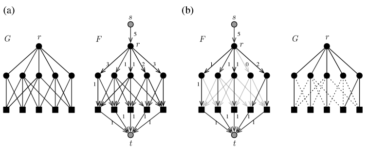
Figure 13: (a) An example of the auxiliary network $F$ (on the right) constructed from $G$ (on the left). Edges from $X$ to $C$ have capacity $1$, all other edges have capacities as shown. (b) On the left, a maximum flow in $F$. Dark edges have flows with shown values and light edges have no flow. On the right, the assignment obtained from this flow.

Proof 6.6.

$(\Rightarrow)$ Suppose $F$ has an $s-t$ flow $f$ of value $|C|$. We denote by $f({u},{v})$ the flow value on the edge $(u,v)$. Since $|C|$ is integral and all capacities are integral, we can assume that flow values of $f$ on all edges are integral. Therefore, for each vertex $c\in C$, $f({c},{t})=1$, which implies that there is exactly one vertex $x\in X$ with $f({c},{x})=1$. We then assign $c\to x$.

Next, we need to verify that in the corresponding tree the congestions of the edges in $E_{r}$ are at most $K$. For each vertex $x\in X$, the number of vertices in $C$ that can be assigned to this $x$ is bounded by $c({r},{x})$. By Equation 1, $\text{cng}(r,x)\leq\text{deg}_{G}(x)+c({r},{x})\,(\alpha-2)\leq K$, which completes the proof of this implication.

$(\Leftarrow)$ Suppose there exist feasible assignments for all vertices in $C$. From this assignment we will construct an $s-t$ flow $f$ for $F$ with value $|C|$. For each vertex $c\in C$, if $c$ is assigned to $x\in X$, then we define $f({x},{c})=1$ and $f({x^{\prime}},{c})=0$ for all $x^{\prime}\in N_{G}(c)\setminus{\left\{x\right\}}$. Next, for each vertex $x\in X$, we define $f({r},{x})=n_{x}$ where $n_{x}$ is the number of vertices in $C$ that are assigned to $x$. Due to the congestion bound on $(r,x)$, we have $n_{x}\leq\frac{K-\text{deg}_{G}(x)}{\alpha-2}$. However, since $n_{x}$ is integral, we have $n_{x}\leq\lfloor\frac{K-\text{deg}_{G}(x)}{\alpha-2}\rfloor=c({r},{x})$. Lastly, we let $f({c},{t})=1$ for each $c\in C$ and $f({r},{s})=|C|$. Clearly, the constructed flow $f$ has value $|C|$, and it satisfies flow conservation and capacity constraints of $F$.

References

- [1] Fernando Alvarruiz Bermejo, Fernando Martínez Alzamora, and Antonio Manuel Vidal Maciá. Improving the efficiency of the loop method for the simulation of water distribution networks. Journal of Water Resources Planning and Management, 141(10):1–10, 2015.
- [2] András A Benczúr and David R Karger. Approximating minimum cuts in time. In Proceedings of the 28th Annual ACM Symposium on Theory of Computing, pages 47–55, 1996.
- [3] Sandeep Bhatt, Fan Chung, Tom Leighton, and Arnold Rosenberg. Optimal simulations of tree machines. In Proceedings of the 27th Annual Symposium on Foundations of Computer Science, SFCS ’86, page 274–282, USA, 1986. IEEE Computer Society.
- [4] Hans Bodlaender, Fedor Fomin, Petr Golovach, Yota Otachi, and Erik Leeuwen. Parameterized complexity of the spanning tree congestion problem. Algorithmica, 64:1–27, 09 2012.
- [5] Hans L. Bodlaender, Kyohei Kozawa, Takayoshi Matsushima, and Yota Otachi. Spanning tree congestion of k-outerplanar graphs. Discrete Mathematics, 311(12):1040–1045, 2011.
- [6] Leizhen Cai and Derek G. Corneil. Tree spanners. SIAM Journal on Discrete Mathematics, 8(3):359–387, 1995.
- [7] E. Dahlhaus, D. S. Johnson, C. H. Papadimitriou, P. D. Seymour, and M. Yannakakis. The complexity of multiterminal cuts. SIAM Journal on Computing, 23(4):864–894, 1994.
- [8] Feodor F. Dragan, Fedor V. Fomin, and Petr A. Golovach. Spanners in sparse graphs. Journal of Computer and System Sciences, 77(6):1108–1119, 2011.
- [9] Yuval Emek and David Peleg. Approximating minimum max-stretch spanning trees on unweighted graphs. SIAM Journal on Computing, 38(5):1761–1781, 2009.
- [10] Sándor P. Fekete and Jana Kremer. Tree spanners in planar graphs. Discrete Applied Mathematics, 108(1):85–103, 2001. Workshop on Graph Theoretic Concepts in Computer Science.
- [11] Wai Shing Fung, Ramesh Hariharan, Nicholas JA Harvey, and Debmalya Panigrahi. A general framework for graph sparsification. In Proceedings of the 43rd Annual ACM Symposium on Theory of Computing, pages 71–80, 2011.
- [12] Zvi Galil. Efficient algorithms for finding maximum matching in graphs. ACM Computing Surveys (CSUR), 18(1):23–38, 1986.
- [13] John E. Hopcroft and Richard M. Karp. An algorithm for maximum matchings in bipartite graphs. SIAM Journal on Computing, 2(4):225–231, 1973.
- [14] Klemens Hägele, Colm Ó Dúnlaing, and Søren Riis. The complexity of scheduling tv commercials. Electronic Notes in Theoretical Computer Science, 40:162–185, 2001. MFCSIT2000, The First Irish Conference on the Mathematical Foundations of Computer Science and Information Technology.
- [15] Samir Khuller, Balaji Raghavachari, and Neal Young. Designing multi-commodity flow trees. Information Processing Letters, 50(1):49–55, 1994.
- [16] Kyohei Kozawa and Yota Otachi. Spanning tree congestion of rook’s graphs. Discussiones Mathematicae Graph Theory, 31(4):753–761, 2011.
- [17] Kyohei Kozawa, Yota Otachi, and Koichi Yamazaki. On spanning tree congestion of graphs. Discrete Mathematics, 309(13):4215–4224, 2009.
- [18] Christian Löwenstein. In the Complement of a Dominating Set. PhD thesis, Technische Universität at Ilmenau, 2010.
- [19] Yoshio Okamoto, Yota Otachi, Ryuhei Uehara, and Takeaki Uno. Hardness results and an exact exponential algorithm for the spanning tree congestion problem. In Proceedings of the 8th Annual Conference on Theory and Applications of Models of Computation, TAMC’11, page 452–462, Berlin, Heidelberg, 2011. Springer-Verlag.
- [20] M.I Ostrovskii. Minimal congestion trees. Discrete Mathematics, 285(1):219–226, 2004.
- [21] Yota Otachi. A Survey on Spanning Tree Congestion, pages 165–172. Springer International Publishing, Cham, 2020.
- [22] Yota Otachi, Hans L. Bodlaender, and Erik Jan Van Leeuwen. Complexity results for the spanning tree congestion problem. In Proceedings of the 36th International Conference on Graph-Theoretic Concepts in Computer Science, WG’10, page 3–14, Berlin, Heidelberg, 2010. Springer-Verlag.
- [23] Arnold L. Rosenberg. Graph embeddings 1988: Recent breakthroughs, new directions. In John H. Reif, editor, VLSI Algorithms and Architectures, pages 160–169, New York, NY, 1988. Springer New York.
- [24] Daniel A Spielman and Shang-Hua Teng. Spectral sparsification of graphs. SIAM Journal on Computing, 40(4):981–1025, 2011.
- [25] Ryo Yoshinaka. Higher-order matching in the linear lambda calculus in the absence of constants is NP-complete. In Jürgen Giesl, editor, Term Rewriting and Applications, pages 235–249, 2005.