Breather Solutions to a Two-dimensional
Nonlinear Schrödinger Equation with Non-local Derivatives

Abstract

We consider the nonlinear Schrödinger equation with non-local derivatives in a two-dimensional periodic domain. For certain orders of derivatives, we find a new type of breather solution dominating the field evolution at low nonlinearity levels. With the increase of nonlinearity, the breathers break down, giving way to wave turbulence (or Rayleigh-Jeans) spectra. Phase-space trajectories associated with the breather solutions are found to be close to that of the linear system, revealing a connection between the breather solution and Kolmogorov-Arnold-Moser (KAM) theory.

I Introduction

Breathers are a broadly-defined class of features that arise in nonlinear dynamical systems, generally describing a family of solutions with strong spatial localization and oscillations in time. Together with solitons, breathers are considered as prototypes for rogue waves that can occur across many fields, such as water waves [1, 2], optics [3], and plasma physics [4]. Mathematically, breathers are fundamental solutions to both continuous field equations and discrete lattice problems. In the former case, breather solutions have been found primarily in one-dimensional (1D) nonlinear partial differential equations, including the Sine-Gordon equation [5], the nonlinear Schrödinger equation (NLS) [6, 1, 2, 3, 4], and the Korteweg–De Vries (KdV) equation [7, 8]. In the latter case, discrete breathers [9] (as counterparts to breathers in continuous fields) have been constructed as solutions to a wide variety of systems, including Josephson Junctions [10, 11] and the Fermi-Pasta-Ulam-Tsingou (FPUT) problem [12]. Unlike their continuous counterparts, discrete breathers haven been studied extensively in problems with more than one dimension.

Another important category of studies regards the spontaneous emergence of breathers (and other types of coherent structures) under the free evolution of a system. These coherent structures include the quasi-solitons [13, 14], quasi-breathers [15], and wave collapses [13, 16, 17] identified in the 1D Majda-McLaughlin-Tabak (MMT) model, as well as the discrete breathers in the FPUT problem [18] and the discrete nonlinear Schrödinger equation [19, 20]. As in the case of constructing exact breather solutions, when considering continuous fields, these studies are predominantly performed for 1D situations. The only exception, to our knowledge, is [21], which identifies a breather solution to the NLS with a potential on a two-dimensional (2D) domain, but the mechanism associated with the breather remains unexplained. In general, very little is known about 2D breathers unless one considers discrete lattice problems.

In this letter, we demonstrate the existence of breather solutions to a family of (non-local) derivative NLS without a potential, realized in a 2D periodic domain (we call such solutions generally as breathers instead of quasi-breathers since the latter, as defined in [15] for periodic domains, are associated with very different physics). In addition to being a novel 2D breather in a continuous field, other remarkable and distinguishing features of the solution include: (1) the breather spontaneously emerges from a stochastic wave field after long-time evolution, not relying on specific initial conditions; (2) the breather appears equivalently for both the focusing and defocusing cases, but exists only in the weak nonlinearity regime. As the nonlinearity of the system increases, we find a breakdown of the breather state with the field relaxing to the Rayleigh-Jeans spectrum (or wave turbulence spectrum if dissipation is included). Further analysis shows that the state trajectory of the breathers is associated with a Kolmogorov-Arnold-Moser (KAM) torus, which is a distorted trajectory of the linear (integrable) system that survives when the nonlinearity level is sufficiently low [22].

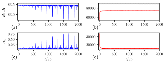
Figure 1: The time series of $H$ (dashed) and $H_{2}$ (solid) for (a) $\varepsilon=0.00071$ and (b) $\varepsilon=0.20$, as well as the corresponding $H_{4}$ for (c) $\varepsilon=0.00071$ and (d) $\varepsilon=0.20$. Note that a low sampling frequency (1 point per $T_{f}$) is used to plot the figure to improve its readability, leading to aliasing. Therefore, only a small portion of all $O(1600)$ peaks are visible.

II Setup of Numerical Experiments

The Majda-McLaughlin-Tabak (MMT) model is a family of nonlinear dispersive wave equations that have been widely used to study wave turbulence [23, 24, 13] and coherent structures [13, 14, 15, 16, 17], due to its effectiveness in representing nonlinear waves in different physical contexts. In the present work, we consider the MMT model in two spatial dimensions, constructed as

$$i\frac{\partial\psi}{\partial t}=|\partial_{\bm{x}}|^{2}\psi+\lambda|\partial_{\bm{x}}|^{\beta/4}\left(\left||\partial_{\bm{x}}|^{\beta/4}\psi\right|^{2}|\partial_{\bm{x}}|^{\beta/4}\psi\right),$$ (1)

where $\psi\equiv\psi(\bm{x},t)$ is a complex scalar, $\bm{x}$ is the spatial coordinates, and $t$ the time. The non-local derivative operator $|\partial_{\bm{x}}|^{\alpha}$ denotes a multiplication by $k^{\alpha}$ on each spectral component in wave number domain, with $k=|\bm{k}|$. The free parameter $\beta$ controls the order of derivatives, and $\lambda=\pm 1$ generates a defocusing/focusing nonlinearity, respectively. Equation (1) is equivalent to a non-local derivative NLS, which can be shown more explicitly after a transformation $\phi=|\partial_{\bm{x}}|^{\beta/4}\psi$, leading to

$$i\frac{\partial\phi}{\partial t}=|\partial_{\bm{x}}|^{2}\phi+\lambda|\partial_{\bm{x}}|^{\beta/2}\left(\left|\phi\right|^{2}\phi\right).$$ (2)

The MMT model (1) can be derived from a Hamiltonian $H=H_{2}+H_{4}$, with

$$\begin{split}H_{2}&=\int\big{|}|\partial_{\bm{x}}|\psi\big{|}^{2}d\bm{x},\\ H_{4}&=\frac{1}{2}\lambda\int\left||\partial_{\bm{x}}|^{\beta/4}\psi\right|^{4}d\bm{x}.\end{split}$$ (3)

The nonlinearity level of the system can be quantified via a parameter $\varepsilon\equiv H_{4}/H_{2}$.

We solve (1) on a 2D periodic domain, starting from an initial field $\psi_{0}\equiv\psi(\bm{x},t=0)$, via a pseudospectral method [24, 25, 26] with $128\times 128$ modes (with higher resolution results available in supplemental material [27]). Our numerical method treats the linear term via an integrating factor, and the nonlinear term via an explicit 4th order Runge-Kutta scheme. The initial field $\psi_{0}$ is set as an exponential form in Fourier space as $\hat{\psi}_{0}(\bm{k})=A\text{exp}[-0.1|k-k_{p}|+i\theta_{\bm{k}}]$, where $k_{p}=4$, and $\theta_{\bm{k}}$ is a random phase that is decorrelated for all $\bm{k}$. In order to investigate dynamics at different nonlinearity levels, we choose a range of $A$ (about 10 values) leading to approximately $\varepsilon\in[0.0005,0.1]$ for each $\beta$ value of interest.

III Results

We start by describing a typical simulation leading to a breather state, with parameters $\beta=3$ and $A=35$ (corresponding to $\varepsilon=0.00071$). Figures 1a and 1c show the long-time evolution of $H_{2}$ and $H_{4}$ from $t=0$ to $2000T_{f}$, with $T_{f}=2\pi$ the period of the fundamental wave mode. The total Hamiltonian $H$, as shown in figure 1a, is well conserved over $2000T_{f}$. After an initial evolution of about $400T_{f}$ with smooth profiles of $H_{2}$ and $H_{4}$, we observe that $H_{4}$ undergoes strong periodic jumps with corresponding dips in $H_{2}$. These jumps are associated with bursts of coherent structures, which are only present at low nonlinearity levels. In contrast, as demonstrated in figures 1b and 1d, the field evolution at a higher nonlinearity ($\varepsilon=0.20$) exhibits smooth profiles of $H_{2}$ and $H_{4}$ over the same time interval.

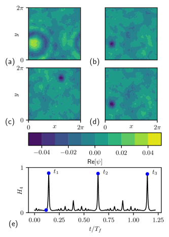
Figure 2: Contour plots of Re$[\psi]$ at $\beta=3$ for $\varepsilon=0.00071$ at various stages of the cycle of the breather (a/b/c/d), corresponding chronologically to the times marked by the blue circles in (e) the time series of $H_{4}$. Note that this plot of $H_{4}$ has sufficient sampling to resolve all features.

The oscillations in $H_{4}$ (and $H_{2}$) correspond to oscillations of a breather. To better visualize this breather state, we plot in figure 2 the real part of $\psi$ at different phases of its oscillations (i.e., different stages of the oscillation pattern in $H_{4}$). Fig. 2a shows the field right before the first jump of $H_{4}$, where a concentric wave appears and later converges into a breather peak seen in Fig. 2b. This peak then collapses, with a second one emerging after about $T_{f}/2$ (according to fig. 2e) at the maximally distant location in the periodic domain, shown in 2c. The cycle then repeats itself with a peak emerging in Fig. 2d (at the same location as in 2a), forming an (oscillating) breather solution coexisting with a stochastic wave background. The smaller peaks of $H_{4}$ seen in Fig. 2e correspond to groups of secondary peaks in $\psi$. We encourage the reader to watch the animation of the full breather cycle (including the secondary peaks) in the supplemental material [27]. From figure 2 we see that the breather oscillates with a period (very close to) $T_{f}$. Therefore, the simulation in figure 1a/c covers $O(1600)$ cycles of the breather, demonstrating a very long (perhaps infinite) time of existence. We note that only a small number of jumps are visible in figure 1a/c simply due to aliasing associated with limited resolution of plotting (see caption of figure 1).

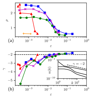
Figure 3: The quantities (a) $\rho$ and (b) $\gamma$ as functions of $\varepsilon$ for $\beta=0$ (orange $+$), $\beta=1$ (green $\bullet$), $\beta=2$ (magenta $\times$), $\beta=3$ (blue $\blacksquare$), and $\beta=4$ (red $\blacktriangle$). The inset of (b) shows fully-developed, angle-averaged wave action spectra at a few nonlinearity levels (for $\beta=3$), with the Rayleigh-Jeans spectral slope of $\gamma=-2$ indicated (dashed).

We next investigate the existence and intensity of the breathers for varying values of $\beta$ and $\epsilon$. To measure the intensity of the breather (relative to the background wave field), we define the peak-to-background ratio as

$$\rho=\frac{\text{avgmax}[|\psi|]}{4\sigma_{|\psi|}},$$ (4)

where the avgmax operator returns the average of the maximum height of primary peaks (as in Fig. 2b/c/d) over many cycles of the breather, and $\sigma_{|\psi|}$ is the total standard deviation of the field $|\psi|$ over space and time. By definition (4), $\rho=2$ corresponds to the typical rogue wave criterion used in many fields [3].

Figure 3a shows the value of $\rho$ obtained for $\beta=0,1,2,3,4$ and $\varepsilon$ across three orders of magnitude. In general, we see that the breather state is present for smaller $\varepsilon$ (i.e., weak nonlinearity) and becomes stronger when $\beta$ is closer to 3. The case with $\beta=0$ (corresponding to NLS) leads to no breathers, indicating a non-local derivative in NLS is necessary for their emergence. We note that when the breathers are not present, the value of $\rho$ is evaluated by taking the average of the maximum of the field $|\psi|$ every $T_{f}/2$ as the numerator in (4).

Furthermore, we examine in figure 3b the slope $\gamma$ of the stationary wave action spectrum $n(\bm{k})\equiv\langle\hat{\psi}(\bm{k})\hat{\psi}^{*}(\bm{k})\rangle$ across all values of $\beta$ and $\varepsilon$. The inset of figure 3b shows a typical example of fully-developed, angle-averaged $n(k)$ for $\beta=2$ and several values of $\varepsilon$. We see that the Rayleigh-Jeans spectrum with $\gamma=-2$ is only achieved at higher nonlinearity when the breather is not present. This trend is generally true for all values of $\beta$ as shown in Figure 3b.

A few additional remarks are in order. First, we note that the breather also emerges for the focusing equation (1) with $\lambda=-1$ under the same conditions. Second, the breather can also be observed under a forced/dissipated system [28], but with the Rayleigh-Jeans spectrum replaced by the wave turbulence spectrum at high nonlinearity levels. Last but not least, we have performed extensive numerical analysis to verify that the breather we observe is not a numerical artifact. This includes the verification of the robustness of our results under symplectic integration, higher resolution, and different dealiasing schemes. Details of all of the above points can be found in the supplemental material [27].

IV Discussion

In this section, we discuss the physical mechanism associated with the breather solution. We start by stating that there exists an exact breather solution to the linear system of (1), i.e., $H_{4}=0$. What we mean precisely is that, starting from an initial condition with a breather peak (say figure 2b), the field propagated by the linear equation returns to the same state after exactly $T_{f}$. This is because the linear system only contains integer frequencies due to the NLS dispersion relation $\omega=k^{2}$, so that $T_{f}$ is the period of the linear system. This fact suggests that the breather solution to the nonlinear system arises from a deformed trajectory of the linear system.

Since visualizing the high-dimensional trajectory is very difficult, we define a projection of the trajectory to some physically meaningful reference field:

$$I_{n}=\left|\frac{\int\psi^{*}_{R}(\bm{x},t_{n})\psi(\bm{x},t)d\bm{x}}{\int\psi^{*}_{R}(\bm{x},t_{n})\psi_{R}(\bm{x},t_{n})d\bm{x}}\right|$$ (5)

where $\psi^{*}_{R}(\bm{x},t_{n})$ is the reference field where a breather peak is present, e.g., taken from $t_{1}$ in figure 2e, and $\psi(\bm{x},t)$ is the solution of either the linear or nonlinear system propagated from $\psi^{*}_{R}(\bm{x},t_{n})$. Figure 4 shows the evolution of $I_{1}$ from both linear and nonlinear systems for a range of four nonlinearity levels (at high nonlinearity in Fig. 4d, $t_{1}$ is taken from an arbitrary time in the quasi-stationary state). It is clear that the linear system evolution exhibits a period of $T_{f}$ in all sub-figures as expected. When the nonlinearity level is low, the trajectory identified by $I_{1}$ shows a small deformation from the linear trajectory, as seen in fig. 4a. Such deformation leads to a high-dimensional quasi-periodic trajectory that is evident from not only the gradual time shift of the $I_{1}$ peak, but also the deviation of $I_{1}$ peak from 1 (indicating completely different background waves). As nonlinearity level increases, we observe an increased deformation of the trajectory, until the linear trajectory is entirely destroyed at high nonlinearity in fig 4d. This trajectory deformation can also be observed in the $(I_{1},I_{2})$ plane in figure 5 (on which the linear trajectory shows an “L” shape due to the orthogonality between $\psi^{*}_{R}(\bm{x},t_{1})$ and $\psi^{*}_{R}(\bm{x},t_{2})$), as well as in animations included the supplemental material [27].

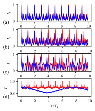
Figure 4: $I_{1}$ evaluated for the nonlinear system $\beta=3$ (blue) and the linear system (red) for (a) $\varepsilon=0.00071$, (b) $\varepsilon=0.0084$, (c) $\varepsilon=0.013$, and (d) $\varepsilon=0.20$.

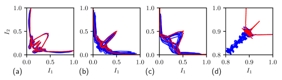
Figure 5: The trajectory of $\psi$ projected on to $I_{1}$ and $I_{2}$ for several fundamental periods of $\psi$ computed via the nonlinear system $\beta=3$ (blue) and the linear system (red) for (a) $\varepsilon=0.00071$, (b) $\varepsilon=0.0084$, (c) $\varepsilon=0.013$, and (d) $\varepsilon=0.20$.

The trajectory deformation visualized above can be connected to Kolmogorov-Arnold-Moser (KAM) theory. If one considers the linear system as the base integrable system, then the nonlinear term is the perturbation added to the system to form a nearly integrable system. According to KAM theory, if the (nonlinear) perturbation is sufficiently small, some trajectories of linear system can be preserved with small deformation to a KAM torus [22]. In our case, these preserved trajectories (i.e., KAM tori) correspond to those associated with the breather solution observed in figure 2. We also note that equation (1) (or more generally the NLS) is a special case on which KAM theory has not been fully understood mathematically, mainly because the base linear system does not contain irrational frequencies (or quasi-periodicity) that are required by the traditional KAM theorem. While most mathematical work of KAM on NLS relies on some way to introduce irrational frequencies, e.g., by including a potential term as in [29], recent progress [30] does show that it is possible to prove the existence of quasi-periodic trajectories for the 2D NLS (without a potential) for small nonlinearity. Our results therefore demonstrate a breather solution associated with the quasi-periodic trajectory if a non-local derivative is included in the NLS. Furthermore, if a different dispersion relation, say $\omega=k^{1/2}$, is prescribed for (1), the KAM theorem is more straightforward to apply (due to quasi-periodicity of the linear system). However, in this case, the breather state we observe is no longer a solution to the linear system, and one would not expect to observe it in the nonlinear system as well. We have confirmed this argument through numerical experiments.

Finally, the current analysis clearly does not resolve all the questions regarding the new 2D breather solution. One critical question is why it arises more strongly for $\beta$ close to 3. For these values of $\beta$, it is clear not only that the trajectories associated with breathers are stable, but also that they lie on some type of quasi-periodic “attractor” [31], such that a variety of initial conditions lead to the breather state. The reason for such dynamical behavior needs to be investigated in future work. In addition, our work provides a clear demonstration of the discrete wave turbulence regime governed by the KAM theory that has long been hypothesized in the literature [32].

V Conclusion

In this paper, we present results regarding a novel breather which spontaneously emerges from a 2D non-local derivative NLS. We show that the breather emerges at low nonlinearity with parameter $\beta$ close to 3. An analysis of phase space trajectory reveals that the trajectory associated with the breather solution is close to that of the linear system, but with quasi-periodicity introduced by the nonlinearity. The numerical findings support an explanation of the breather solution by the KAM theory, in the sense that a trajectory with the breather solution of the linear system is deformed but preserved when a small nonlinearity is introduced.