Enhancing quality and speed in database-free neural network reconstructions of undersampled MRI with SCAMPI

Abstract

Purpose: We present SCAMPI (Sparsity Constrained Application of deep Magnetic resonance Priors for Image reconstruction), an untrained deep Neural Network for MRI reconstruction without previous training on datasets. It expands the Deep Image Prior approach with a multi-domain, sparsity-enforcing loss function to achieve higher image quality at a faster convergence speed than previously reported methods. Methods: Two-dimensional MRI data from the FastMRI dataset with Cartesian undersampling in phase-encoding direction were reconstructed for different acceleration rates for single coil and multicoil data. Results: The performance of our architecture was compared to state-of-the-art Compressed Sensing methods and ConvDecoder, another untrained Neural Network for 2D MRI reconstruction. SCAMPI outperforms these by better reducing undersampling artifacts and yielding lower error metrics in multicoil imaging. In comparison to ConvDecoder, the U-Net architecture combined with an elaborated loss-function allows for much faster convergence at higher image quality. SCAMPI can reconstruct multicoil data without explicit knowledge of coil sensitivity profiles. Moreover, it is a novel tool for reconstructing undersampled single coil k-space data. Conclusion: The presented approach avoids overfitting to dataset features, that can occur in Neural Networks trained on databases, because the network parameters are tuned only on the reconstruction data. It allows better results and faster reconstruction than the baseline untrained Neural Network approach.

Keywords: Convolutional Prior, Magnetic Resonance Imaging, Deep Image Prior, DIP, Sparsity, Domain Transform Sparsity, Compressed Sensing, CNN, learning-free, untrained, Neural Network

1 Introduction

Increasing acquisition speed is one major goal of ongoing research in Magnetic Resonance (MR) Imaging. Two common approaches are widely used in the clinical routine to accelerate data acquisition. Both are based on extensive undersampling of the MR signal in the Fourier domain. The first is Parallel Imaging (PI), which exploits the redundancy of data received by several radio-frequency coils [1, 2, 3, 4]. It can be applied to 2D and 3D imaging and can be combined with techniques like simultaneous multislice excitation [5]. The second one introduces sparsity regularization into the image reconstruction process and is known as Compressed Sensing (CS) [6]. In combination (PICS), both techniques can achieve high acceleration rates [7, 8]. Nonetheless, the reconstruction task in general is an ill-posed optimization problem. Solving it often requires computationally intense iterative algorithms, which limits its application, for example in fields such as real time imaging. Thus, the need for fast image reconstruction has been one reason for the advent of Neural Networks and deep learning strategies in the application of MRI reconstruction [9, 10, 11].

On a high abstraction level, two classes of methods that use Neural Networks can be distinguished. Data-driven machine learning algorithms require large datasets in order to tune network parameters, so that they ‘learn’ to reconstruct high-quality images from undersampled measurements. Several studies have shown that deep learning approaches outperform the aforementioned state-of-the-art methods, not only in terms of reconstruction speed, but also in terms of image quality [12, 13]. Despite remarkable results, data-based approaches have serious limitations when generalizing from training data: Overfitting to particular features of the training data set can lead to bias and limit generalization when posed with previously unseen data in new applications. Upon inference on new data, this can lead to hallucination of features that are common in the training data set [14]. Vice versa, it may cause removal of actual features that were never seen before in the training data, which can be fatal for diagnostic imaging [13]. Moreover, reconstruction quality of a well-trained Neural Network deteriorates when confronted with new imaging properties, such as different sampling patterns or signal-to-noise ratio of the underlying data [15, 16].

Additionally, high quality ground truth data can be scarce or physically impossible to acquire. Therefore, various strategies of unsupervised learning have emerged, that do not require fully sampled reference data, but can be trained on datasets of undersampled measurements [17, 18, 19, 20]. However, they do not change the general strategy to infer image properties from a training dataset to a new reconstruction task.

The second approach that uses Neural Network algorithms does not require training databases and fits the model parameters only to the individual scan’s data [22]. For example, the RAKI [23] architecture extends GRAPPA’s [1] linear convolution kernels by multiple layers of scan-specifically trained convolutions, linked by rectified linear units (ReLU). The authors point out that non-linear functions with few degrees of freedom are better at approximating higher-dimensional linear functions and show that RAKI has superior noise-resilience and better reconstruction performance than GRAPPA. In both algorithms, the convolution kernel parameters are optimized to represent a mapping function from undersampled zero-filled k-space data $\mathbf{k}_{0}$ to reconstructed $\mathbf{k}$, where the missing lines are calculated from local correlations to neighboring multichannel k-space points. A similar approach is pursued by Wang et al. [24], who use an unrolled Convolutional Neural Network (CNN) with data-consistency layers to map from $\mathbf{k}_{0}$ to $\mathbf{k}$.

In the present paper, we focus on a different reconstruction strategy, coined Deep Image Prior (DIP), which originates from the field of image restoration [25]. Similar to MR-reconstruction, image restoration tasks can be formulated as an optimization problem. Instead of using a gradient descent method to search for an optimal solution $\mathbf{x}$ directly in the image space, DIP shifts the search to the parameter space of the Neural Network. The network weights are optimized, until the network is able to reconstruct the final image out of a fixed random noise input sample. Ulyanov et al. showed, that a U-Net [26] architecture is biased to prefer the reconstruction of natural images over less structured data. Therefore, when training the network to reconstruct a corrupted image $\mathbf{x}_{0}$, starting from randomly initialized parameters, it can be observed that the solution $\mathbf{x}$ is reached with lower impedance than $\mathbf{x}_{0}$ during the training [25]. The architecture serves as a statistical prior of $\mathbf{x}$. DIP has shown competitive performance in image restoration tasks such as inpainting, denoising and super-resolution.

In MR reconstruction this is leveraged for non-linear interpolation of missing k-space data. Previous studies investigated this approach in combination with learning from reference data [27, 28, 29] or to reconstruct dynamic MRI data [30, 31]. Other authors studied the combination of DIP with TV regularization in non-MRI context [33, 34, 35] or combined with federated learning for pre-training [36] or in quantitative MRI [37]. Darestani et al. investigated variations of the network architecture and their implications on reconstruction performance and presented ConvDecoder for reconstruction of 2D MRI with Cartesian undersampling [32].

In our study, we utilize the original U-Net architecture suggested for DIP [25] and investigate, how different sparsity regularization terms in the loss function improve reconstruction results. In the following, we illustrate the resulting SCAMPI architecture and demonstrate that our approach outperforms state-of-the art parallel imaging MRI reconstruction methods and can also be applied in single channel reconstruction. In comparison to ConvDecoder, it shows improved reconstruction quality with much fewer iterations.

2 Methods

2.1 The SCAMPI architecture

Undersampling reconstruction can be illustrated as filling the missing data points of the undersampled measurement

$$\mathbf{k}_{0}=\mathcal{P}\,\mathbf{k}.$$ (1)

Here, ${\mathbf{k}\in\mathbb{C}^{n_{c}\times N_{x}\times N_{y}}}$ is the full set of spatial frequency data. $n_{c}$ is the number of coil channels and $N_{x,y}$ the number of k-space coefficients in readout and phase encoding direction. $\mathcal{P}$ is the undersampling projection operator, effectively setting certain lines in phase-encoding direction of $\mathbf{k}$ to zero.

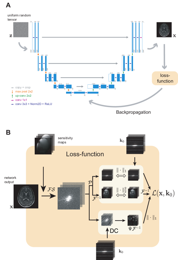
DIP on the other hand has shown promising results in various image reconstruction tasks. However, convolutional layers, that are used in DIP, favor natural images by imposing local spatial correlations on different length scales. But the k-space results from an integral transform and does not show these local structures. Hence, the reconstruction is not searched directly in k-space by our approach. Instead, the U-Net [26] $f$ operates in image space. The parameter space of network weights $\theta$ is searched, such that an image ${\mathbf{x}=f_{\theta}(\mathbf{z})}$ is built from a fixed but randomly initialized input ${\textbf{z}\in\mathbb{R}^{2\times N_{x}\times N_{y}}}$. The resulting network architecture is shown in Fig. 1 A. Details on the layer parameters are provided in Supplementary Materials Tab. 1.

$\mathbf{k}$ is then obtained from $\mathbf{x}$ as the coil sensitivity-weighted Fourier transform ${\mathbf{k}=\mathcal{FS}\mathbf{x}}$, where $\mathcal{F}$ is the Fourier transform and $\mathcal{S}$ represents the coil sensitivity profiles. To iteratively find the optimal k-space reconstruction ${\hat{\mathbf{k}}=\mathcal{FS}\hat{\mathbf{x}}=\mathcal{FS}f_{\hat{\theta}}(\mathbf{z})}$, the parameters $\theta$ of the network $f$ are optimized, such that

$$\hat{\theta}=\mathrm{arg}\,\underset{\theta}{\mathrm{min}}\;\mathcal{L}(f_{\theta}(\mathbf{z}),\mathbf{k}_{0})\;.$$ (2)

Here, $\mathcal{L}$ is a cost function, which is further elaborated in Sec. 2.1.1. For optimization of the network weights, the ADAM [38] algorithm with a learning rate $l$ is used. The developed reconstruction algorithm is summarized in Algorithm 1. Fourier transforming the network output before passing it to $\mathcal{L}$ allows to implement a loss functional that compares $\mathbf{k}$ against the measured $\mathbf{k}_{0}$, while using the network’s convolutions in the image domain as an appropriate prior for the image statistics and spatial correlations.

After stopping the iteration, the final multicoil reconstruction is given by $\hat{\mathbf{k}}$ after ensuring data-consistency (DC) with the sampled k-space points $\mathbf{k}_{0}$ (s. Sec. 2). The DC function in Eq. (4) is formalized for each data point $i$ by

$$\left(\mathrm{DC}(\hat{\mathbf{k}},\mathbf{k}_{0};\mathcal{P})\right)_{i}=\left\{\begin{aligned} &(\mathbf{k}_{0})_{i}\quad&&\mathrm{if}\;(\mathcal{P})_{i}=1\\ &(\hat{\mathbf{k}})_{i}\quad&&\mathrm{else.}\end{aligned}\right.$$ (3)

Finally, the image space reconstruction is obtained by phase-sensitive combination of the Fourier transform of the multicoil k-space data, as described by Roemer et al. [39].

Algorithm 1 k-Space reconstruction with SCAMPI.

Undersampled k-space ${\mathbf{k}_{0}\in\mathbb{C}^{n_{c}\times N_{x}\times N_{y}}}$, number of epochs $n$, learning rate $l$

Estimate coil sensitivity profiles $\mathcal{S}$ from $\mathbf{k}_{0}$ with ESPIRiT

Randomly initialize ${\mathbf{z}\in\mathbb{R}^{2\times N_{x}\times N_{y}}}$ and $\theta_{i=0}$

for $n$ iterations do

     $\mathbf{x}_{i}=f_{\theta_{i}}(\mathbf{z})$ with $\mathbf{x}\in\mathbb{C}^{N_{x}\times N_{y}}$

     $\theta_{i+1}\leftarrow\operatorname{ADAM}\left(\theta_{i},\,\mathcal{L}(\mathbf{x}_{i},\mathbf{k}_{0}),\,l\right)$

end for

$\hat{\mathbf{x}}=f_{\theta_{n}}(\mathbf{z})$

$\hat{\mathbf{k}}=\mathrm{DC}(\mathcal{FS}\hat{\mathbf{x}},\mathbf{k}_{0})$

Final reconstruction $\hat{\mathbf{k}}\in\mathbb{C}^{n_{c}\times N_{x}\times N_{y}}$

Figure 1: The SCAMPI architecture uses A a U-Net with 2D convolutions conv 3x3, where 3x3 describes the 2D convolutional kernel’s size. The number of filter maps is depicted above the layers and reported in Supplementary Materials, Tab. 1. 2D normalization layers and Rectified Linear Units(ReLU) are placed between the convolutional layers. Maximum pooling (max pool 2x2) with kernel size 2x2 is used for down-sampling. Bilinear interpolation is used for up-sampling (up-conv 2x2). Zero-padding is used in convolutional layers to preserve the input images’ sizes. U-Net’s final output layer returns a $\mathbb{R}^{2\times N_{x}\times N_{y}}$ tensor. The first dimension’s two channels are treated as real and imaginary part of the image $\mathbf{x}\in\mathbb{R}^{N_{x}\times N_{y}}$. B In the loss function $\mathcal{L}$, the transformed network output ${\mathbf{k}=\mathcal{FS}\mathbf{x}}$ is compared to $\mathbf{k}_{0}$ in the measured data-points points and subjected to a sparsity constraint (here, L1 norm of wavelet coefficients is shown as an example).

2.1.1 Loss function

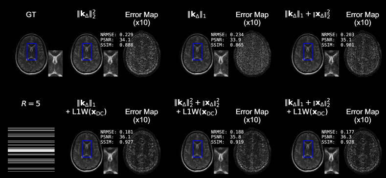
During the training process as given by Eq. (2), the network parameters $\theta$ are tuned by gradient backpropagation from the loss-function $\mathcal{L}$. To meet the requirements for the non-linear k-space interpolation, we heuristically assembled a dedicated loss function. Each term has a specific impact on the overall reconstruction result. The L1 norm in k-space is more resilient to outliers and causes errors in the k-space center to be less significant. Furthermore, we incorporated a L2 loss term in image domain to enforce appearance-consistency [40]. For additional sparsity regularization, we implemented Total Variation (TV), as well as L1 norm of the wavelet coefficients (L1W).

We evaluated different combinations of loss terms for optimized reconstruction of an undersampled ($R=5$) multicoil ($n_{c}=12$) image from the FastMRI brain dataset [41] (s. Sec. 2 for details). Reconstruction quality was assessed visually and quantitatively, using NRMSE, PSNR and SSIM (as introduced in Sec. 2.4), which were calculated from magnitude images of the reconstructions against the ground truth (GT) reference image. A selection of results is depicted in Fig. 2. Ascertaining data-fidelity with L1 leads to noisier images, than with L2 penalty. However, when combining multiple loss terms, the combination of data-fidelity with L1, appearance-fidelity in image space with L2 and sparsity regularization achieves the best results.

Figure 2: Multi-coil ($n_{c}=12$) reconstruction of undersampled k-space data (${R=5}$) with U-Net and different loss terms. The shorthand notations denote: ${\mathbf{x}_{\Delta}=\mathcal{PFS}\mathbf{x}-\mathbf{k}_{0}}$, ${\mathbf{k}_{\Delta}=\mathcal{F}^{-1}\left(\mathcal{PFS}\mathbf{x}-\mathbf{k}_{0}\right)}$, ${\mathbf{x}_{\mathrm{DC}}=\mathcal{F}^{-1}\mathrm{DC}(\mathcal{FS}\mathbf{x},\mathbf{k}_{0})}$. Error Map shows relative difference ($\times 10$) to the Ground Truth (GT) reconstruction. The undersampling pattern in k-space is illustrated below the GT image. Quantitative error measures NRMSE, PSNR and SSIM, compared to the GT are reported next to each reconstruction image. Inlay image shows zoom-in of the periventricular region (blue frame).

Based on these results, we proceed with the combination of loss terms, that is depicted in Fig. 1 B and is given as

$$\mathcal{L}(\mathbf{x},\mathbf{k}_{0})= \eta_{1}\,\left\|\mathcal{PFS}\mathbf{x}-\mathbf{k}_{0}\right\|_{1}$$ (4)

$$+ \eta_{2}\,\left\|\mathcal{F}^{-1}\left(\mathcal{PFS}\mathbf{x}-\mathbf{k}_{0}\right)\right\|_{2}^{2}$$

$$+ \rho\,\mathcal{R}\left[\mathcal{F}^{-1}\mathrm{DC}(\mathcal{FS}\mathbf{x},\mathbf{k}_{0})\right]\;.$$

The first two terms of $\mathcal{L}$ assert the reconstruction’s data and appearance fidelity to $\mathbf{k}_{0}$. The last term enforces transform-domain sparsity of $\mathbf{x}$. The DC function in the last term proved necessary to avoid divergence of the loss during the first iterations of training, since the random input is not sparse in the transform domain. Settings for the weighting parameters $\eta_{1,2}$ and $\rho$ are reported in Sec. 2.

2.1.2 Calibration-free reconstruction

For multicoil data with $n_{c}$ coils, the number of output filter maps of the network can be adjusted to output ${\mathbf{X}\in\mathbb{C}^{n_{c}\times N_{x}\times N_{y}}}$ instead of ${\mathbf{x}\in\mathbb{C}^{N_{x}\times N_{y}}}$. This allows to build an algorithm that does not require previously calibrated coil sensitivity profiles, but inherently outputs a multicoil k-space approximation ${\mathbf{k}=\mathcal{F}\mathbf{X}}$. Then, ${\mathbf{x}\in\mathbb{C}^{N_{x}\times N_{y}}}$ is given as the root sum of squares of $\mathbf{X}$.

2.2 Implementation of algorithms

Python 3 was used for all algorithms and simulations described in this work. The SCAMPI network and the training pipeline were built using the PyTorch library [42]. The U-Net implementation builds on publicly available code [43]. Details on the layer parameters can be found in Supplementary Materials, Tab. 1. All complex-valued tensors were implemented inside the network as tensors in $\mathbb{R}^{2}$, representing real and imaginary part of the data. If the output-tensor included coil data (in the calibration-free case), the complex and coil channels were stored in a shared channel inside the tensor, i.e., a multicoil image with $n_{c}$ coils is represented as a $2\,n_{c}$ channel tensor. The coil sensitivity profiles $\mathcal{S}$, that are required for some of the reconstructions were obtained via ESPIRiT [44] calibration, which was implemented in BART [45].

SCAMPI reconstructions were generated by $1000$ iterative steps of updating the network weights. The learning rate $l$ as well as the weighting parameters of the loss function in Eq. (4), $\eta_{1,2}$ and $\rho$ were tuned heuristically and are reported in tab. 1. To determine the required number of iterations, the training loss of the reconstruction against the undersampled measurement data was recorded during training. $1000$ epochs were determined as a good trade-off between reconstruction time and quality (see Suppl., Sec. S1.3 for details).

For all reported comparisons we used the PICS algorithm implemented in SigPy [46], which optimizes

$$\min_{\mathbf{x}}\frac{1}{2}\left\|\mathcal{PFS}\mathbf{x}-\mathbf{k}_{0}\right\|_{2}^{2}+\lambda\;\mathrm{L1W}[\mathbf{x}]$$ (5)

via iterative soft thresholding. We iterated for $500$ steps and heuristically tuned weighting parameter $\lambda=0.5$ of the sparsity regularization term L1W.

For TV, we used a finite gradient operator with a one-pixel-shift in both spatial dimensions. For L1W, we used a wavelet transformation $\Psi$ with Daubechies-Wavelets (D4) as basis functions and decomposition level of $5$.

For ENLIVE, we chose the parameters ($a=240,b=40,m=1$), as introduced by [47]. We chose the number of iterations $i=9$, because for more iterations we observed an increase of high frequency noise, as described by the authors.

For ConvDec, we used the settings, given in the code example by the authors for the knee images: $160$ channels, an input size of ($8$, $4$) and a kernel size of $3$ [32]. For the brain images, we set the input size to ($4$, $4$), due to the smaller and quadratic matrix size of the k-space data. The network was optimized with ADAM optimizer and learning rate $l=0.008$ for $20000$ iterations.

Reconstructions were performed on a Linux system with Intel(R) Xeon(R) Silver 4214R CPU and Nvidia(R) Titan RTX GPU.

Table 1: Chosen hyperparameters for SCAMPI reconstructions presented in Sec. 3. Learning Rate $l$ and weighting factors $\eta_{1}$ for k-space, $\eta_{2}$ for image domain loss and $\rho$ for sparsity constraints Total Variation (TV) and L1 norm of Wavelets (L1W).

Multicoil - with coil sensitivities
			TV		L1W
R	$\eta_{1}$	$\eta_{2}$	$l$	$\rho$	$l$	$\rho$
3	20	1	0.03	$3\times 10^{-8}$	0.03	$3\times 10^{-8}$
5	20	1	0.03	$3\times 10^{-8}$	0.03	$5\times 10^{-8}$
8	20	1	0.03	$5\times 10^{-9}$	0.03	$5\times 10^{-9}$
Multicoil - without coil sensitivities
			TV		L1W
R	$\eta_{1}$	$\eta_{2}$	$l$	$\rho$	$l$	$\rho$
3	20	1	0.03	$1\times 10^{-8}$	0.03	$1\times 10^{-7}$
5	20	1	0.01	$5\times 10^{-8}$	0.01	$8\times 10^{-8}$
8	20	1	0.01	$3\times 10^{-8}$	0.01	$8\times 10^{-8}$
Single coil
			TV		L1W
2	20	1	0.01	$5\times 10^{-6}$	0.01	$5\times 10^{-6}$
3	20	1	0.01	$5\times 10^{-6}$	0.01	$5\times 10^{-6}$

2.3 Reconstruction data

Data used in the preparation of this article were obtained from the NYU fastMRI initiative database (fastmri.med.nyu.edu) [48, 41]. We did not perform experiments on humans or human tissues.

2.3.1 Multicoil data

Reconstruction performance of the suggested design was evaluated on an axial T2-weighted image from the fastMRI brain dataset (file name file_brain_AXT2_209_6001331). One bottom slice from the fully sampled multi-slice dataset was taken as the ground truth (GT) and retrospectively undersampled. To save memory, the field of view was cropped to $396^{2}$ pixels. For Cartesian undersampling, we pseudo-randomly selected readout lines from a Gaussian probability density distribution with maximum in k-space center. The sampling algorithm was designed to assure that the central $18$ lines were always sampled. Multicoil (${n_{c}=12}$) reconstruction performance was assessed for ${R=3,5,8}$. The robustness of our results was investigated on a subset of $200$ different samples, selected randomly from the FastMRI brain dataset (validation set). Different MRI contrast modalities (FLAIR, T1, T2) were present in the subset. From each multi-slice dataset, the lowest slice was selected and cropped to shape $N^{2}$, where ${N=\min(N_{x},N_{y})}$ and $N_{x,y}$ is the number of pixels in the two spatial dimensions. For each sample, a new undersampling pattern was randomly generated. Reconstruction was performed as outlined for the single sample described above, and error metrics of SCAMPI and baseline reconstructions were compared.

2.3.2 Single coil data

Furthermore, single coil (${n_{c}=1}$) reconstruction for ${R=2,3}$ was investigated on a central slice from the FastMRI single coil knee validation dataset [41] (file1001221).

A statistical analysis of the reconstruction quality at ${R=2,3}$ was performed on $200$ randomly selected images from the dataset, which were processed in the same manner as the multicoil data described above.

2.4 Image error metrics

For quantitative evaluation of our results we used the Normalized Root Mean Squared Error

$$\mathrm{NRMSE}[\mathbf{a},\mathbf{b}]=\frac{\mathrm{RMSE}[\mathbf{a},\mathbf{b}]}{\bar{a}}$$ (6)

and Peak Signal Noise Ratio

$$\mathrm{PSNR}[\mathbf{a},\mathbf{b}]=20\cdot\log_{10}{\left(\frac{\max[\mathbf{a}]}{\textrm{RMSE}[\mathbf{a},\mathbf{b}]}\right)}\;,$$ (7)

where $i$ runs over all $N$ values $a_{i},b_{i}$ of the input images $\mathbf{a}$ and $\mathbf{b}$, $\bar{a}$ denotes the mean value of $\mathbf{a}$ and $\mathrm{RMSE}$ the Root Mean Squared Error.

Results were also compared to the GT with the Structural Similarity Index

$$\operatorname{SSIM}[\mathbf{a},\mathbf{b}]=\frac{\left(2\mu_{\mathbf{a}}\mu_{\mathbf{b}}+c_{1}\right)\left(2\sigma_{\mathbf{a}\mathbf{b}}+c_{2}\right)}{\left(\mu_{\mathbf{a}}^{2}+\mu_{\mathbf{b}}^{2}+c_{1}\right)\left(\sigma_{\mathbf{a}}^{2}+\sigma_{\mathbf{b}}^{2}+c_{2}\right)}\;,$$ (8)

where $\mu_{\mathbf{a},\mathbf{b}}$ are the averages, $\sigma_{\mathbf{a},\mathbf{b}}$ the variances and $\sigma_{\mathbf{a}\mathbf{b}}$ is the covariance between $\mathbf{a}$ and $\mathbf{b}$.

The parameters ${c_{i}=(k_{i}L)^{2}}$ for $i=1,2$ are determined by the dynamic range $L$ of the images’ pixel values and fixed parameters ${k_{1}=0.01}$ and ${k_{2}=0.03}$.

3 Results

In the following section, we demonstrate our reconstruction results on MR data with random Cartesian undersampling in phase-encoding direction and a comparison against baseline methods. Details on the evaluated reconstruction data and parameters are reported in Sec. 2.

3.1 Parallel Imaging Reconstructions

We reconstructed an arbitrarily chosen sample from the FastMRI brain dataset [41], which was undersampled at various acceleration rates $R$.

3.1.1 Calibrated reconstruction using coil-maps

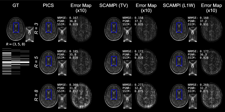
We compare the SCAMPI approach that uses ESPIRiT-estimated coil sensitivity profiles against PICS, which also requires sensitivity map estimates.

Details on parameters are reported in Sec. 2. PICS showed better results with L1W regularization, which is compared against SCAMPI with TV or L1W regularization in Fig. 3.

For both regularization terms, TV and L1W, SCAMPI shows less residual error in the error map and better image quality metrics than the PICS reconstruction.

Figure 3: Comparison of PICS (L1W regularization) and SCAMPI (TV or L1W) reconstruction for different acceleration rates $R$. Error Map shows relative difference ($\times 10$) to the Ground Truth (GT). The undersampling pattern in k-space for different $R$ is illustrated below the GT image. Quantitative error measures NRMSE, PSNR and SSIM, compared to the GT are reported next to each reconstruction. Inlay image shows zoom-in of the periventricular region (blue frame).

3.1.2 Calibration-free reconstruction

As noted in Sec. 2.1.1, the SCAMPI method can be adapted to allow a calibration-free reconstruction, i.e., without requiring ESPIRiT-estimated coil sensitivity profiles.

Figure 4: Root sum of squares of calibration-free reconstruction with ENLIVE, ConvDecoder ($20000$ iterations) and SCAMPI ($1000$ iterations) with Total Variation (TV) sparsity regularization for different acceleration rates $R$. No coil sensitivity estimates are used for reconstruction. Error Map shows relative difference (x10) to the Ground Truth (GT). The undersampling pattern in k-space for $R=(3,\,5)$ is illustrated below the GT image. Quantitative error measures NRMSE, PSNR and SSIM, compared to the GT are reported next to each reconstruction. The Inlay image shows a zoom-in of the periventricular region (blue frame).

In this case, magnitude images are obtained from the multicoil images by calculating the root sum of squares.

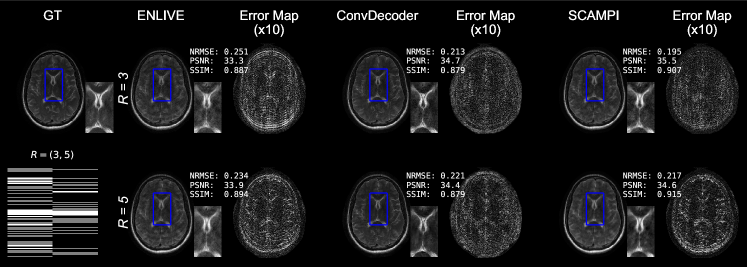
As a baseline, we compare against other calibration-less reconstruction methods: ENLIVE [47], a low-rank based method and ConvDecoder [32], another DIP-based approach, that does not use sparsity-regularization. Details on (hyper)parameter settings are described in Sec. 2.2. To filter random noise in the low signal-region outside the subject’s anatomy, a signal threshold was applied to the images.

Reconstruction results are displayed in Fig. 4. As can be seen from the residual error maps and the image metrics, calibration-free SCAMPI can achieve better reconstruction results than the baseline methods ENLIVE and ConvDecoder. Note that for these results, SCAMPI is iterated 20-times fewer than ConvDecoder, resulting in higher reconstruction speed of ca. $98\,\mathrm{s}$ versus ca. $21\,\mathrm{min}$. A comparison with Fig. 3 shows, that the best reconstruction results with less residual artifacts can be achieved with the SCAMPI algorithm using coil sensitivity information.

3.1.3 Statistical analysis

A statistical analysis was performed on a subset of $200$ samples from the FastMRI dataset, as described in Sec. 2.3. Reconstruction was performed for PICS, ENLIVE, ConvDecoder and SCAMPI (with and without calibration). Details on reconstruction parameters are described in Sec. 2.2, for simplicity and to illustrate the robustness of SCAMPI, the settings for ${R=3}$ were used for all ${R=3,5,8}$ in this analysis. As can be seen from tab. 2, the best image metrics are achieved with the calibrated SCAMPI reconstruction. The calibration-free SCAMPI network also outperforms the reference method ConvDecoder, except in NRMSE and PSNR at ${R=8}$.

In general, image metrics are poorer than in the preceding sections for different reconstruction algorithms. This implies that the previously presented sample ranks among those with the lowest reconstruction error. It should be noted, though, that the FastMRI dataset consists of routine clinical scans, including noisy and flawed measurements or localizer images with low resolution. The sample which was presented above, was selected by visual appearance. This already ascertains a minimum level of image quality. A selection by perceived quality was not done for the full data set, which can explain the higher mean error. Furthermore, especially for noisy GT images, the practical significance of high error metrics between reconstruction and GT can be questioned. A smooth reconstruction might not approximate well to a noisy GT but might actually be preferable in terms of diagnostic quality, if the higher quantitative errors stem from lacking approximation to the random noise in the GT.

Table 2: Mean image quality metrics for PICS (L1W regularization), ENLIVE, ConvDecoder and SCAMPI (TV regularization) on a random subset of $200$ samples from the FastMRI multicoil brain dataset. Error margins denote $95\%$ confidence interval.
^∗: calibration-free. ^∗∗: coil-calibrated

R	Method	NRMSE	PSNR	SSIM
3	PICS	0.169 ± 0.016	34.83 ± 0.51	0.8894 ± 0.0088
	ENLIVE	0.2159 ± 0.0070	32.22 ± 0.36	0.8641 ± 0.0074
	ConvDecoder	0.1760 ± 0.0080	34.11 ± 0.43	0.8672 ± 0.0078
	SCAMPI∗	0.1653 ± 0.0046	34.47 ± 0.36	0.8911 ± 0.0058
	SCAMPI∗∗	0.1425 ± 0.0063	35.96 ± 0.45	0.9181 ± 0.0065
5	PICS	0.271 ± 0.018	30.53 ± 0.44	0.8291 ± 0.0097
	ENLIVE	0.331 ± 0.010	28.47 ± 0.29	0.815 ± 0.0068
	ConvDecoder	0.2378 ± 0.0090	31.46 ± 0.40	0.8312 ± 0.0090
	SCAMPI∗	0.2560 ± 0.0077	30.71 ± 0.34	0.8489 ± 0.0073
	SCAMPI∗∗	0.2173 ± 0.0088	32.26 ± 0.41	0.8765 ± 0.0078
8	PICS	0.400 ± 0.023	27.00 ± 0.36	0.7620 ± 0.0099
	ENLIVE	0.427 ± 0.011	26.22 ± 0.22	0.7800 ± 0.0065
	ConvDecoder	0.311 ± 0.010	29.08 ± 0.37	0.7963 ± 0.0097
	SCAMPI∗	0.367 ± 0.010	27.57 ± 0.28	0.8033 ± 0.0076
	SCAMPI∗∗	0.315 ± 0.010	28.94 ± 0.33	0.8278 ± 0.0084

3.2 Single coil imaging

We studied the reconstruction of single coil MR data with SCAMPI and compared it with CS, ENLIVE and ConvDecoder. Hyperparameters for the reconstruction are reported in Sec. 2. The resulting reconstructions are illustrated in Fig. 5.

Figure 5: Undersampled single coil reconstruction for SCAMPI (L1W regularization, $1000$ iterations) and reference methods ENLIVE, CS (L1W-regularization) and ConvDecoder ($20000$ iterations). Quantitative image metrics NRMSE, PSNR and SSIM are reported next to the images. Relative difference (x10) to Ground Truth (GT) is shown right to each reconstruction. In the panel below the GT, undersampling patterns at $R=2$ and $R=3$ are depicted. Inlay image shows zoom-in of the knee joint region (blue frame).

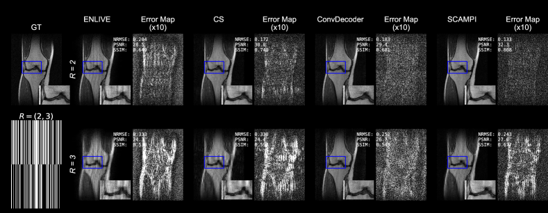
The results in Fig. 5 demonstrate that ENLIVE is ineffective in reducing undersampling artifacts, when used with a single coil. In the CS reconstruction, the undersampling artifacts are better suppressed, but the residual error indicates over-smoothing of the reconstruction. On the other hand, ConvDecoder yields visually appealing reconstructions that appear to remove undersampling artifacts. However, analysis of the error map reveals more random noise, than in the other reconstruction, which leads to inferior image metrics. In contrast, SCAMPI exhibited the best reconstruction outcomes (with similar results for TV and L1W regularization) at ${R=2}$. For ${R=3}$, artifacts in the ConvDecoder reconstruction appear stronger suppressed than in the SCAMPI reconstruction. However, the residual noise in the reconstruction leads to inferior image metrics. To quantify the noise in the reconstructions, we estimated the $\text{SNR}=\frac{\mu}{\sigma}$, where $\mu$ is the average image signal and $\sigma$ the signal variance in a homogenous, low signal region outside the subject’s leg. As can be seen from tab. 3, the SNR is lower for the ConvDecoder reconstruction than for the other reconstructions.

Table 3: SNR for various algorithms, estimated from variance in three different low-signal regions in the single-coil knee reconstruction. Reported values denote mean ± standard error.

R	Algorithm	SNR
n/a	Ground Truth	8.150 ± 0.056
2	ENLIVE	14.7 ± 2.4
	CS	7.58 ± 0.24
	ConvDecoder	6.17 ± 0.44
	SCAMPI (L1W)	10.74 ± 0.23
3	ENLIVE	20.8 ± 5.1
	CS	6.01 ± 0.15
	ConvDecoder	4.95 ± 0.33
	SCAMPI (L1W)	13.03 ± 0.29

Statistical analysis

Statistical analysis was performed on a subset of $200$ samples from the FastMRI singlecoil knee dataset, as described in Sec. 2.3. Reconstruction was performed with the parameter settings reported in Sec. 2.2.

Table 4: Mean image quality metrics for CS (L1W regularization), ENLIVE, ConvDecoder and SCAMPI (L1W regularization) on a random subset of $200$ samples from the FastMRI singlecoil knee dataset. Error margins denote the $95\%$ confidence interval.

R	Method	NRMSE	PSNR	SSIM
2	CS	0.264 ± 0.013	30.34 ± 0.57	0.735 ± 0.017
	ENLIVE	0.280 ± 0.012	29.75 ± 0.55	0.66 ± 0.014
	ConvDecoder	0.297 ± 0.017	29.49 ± 0.66	0.677 ± 0.020
	SCAMPI	0.242 ± 0.013	31.22 ± 0.62	0.771 ± 0.015
3	CS	0.331 ± 0.012	28.22 ± 0.49	0.639 ± 0.020
	ENLIVE	0.337 ± 0.012	28.08 ± 0.50	0.575 ± 0.017
	ConvDecoder	0.361 ± 0.017	27.65 ± 0.60	0.579 ± 0.023
	SCAMPI	0.302 ± 0.012	29.09 ± 0.52	0.680 ± 0.019

Tab. 4 demonstrates, that the best reconstruction metrics are achieved by the SCAMPI algorithm. Also, the average error metrics for some of the methods are higher than for the individual image presented above. Possible reasons have been discussed in the multichannel case (s. Sec. 3.1.3).

4 Discussion and Conclusion

The application of SCAMPI for reconstruction of undersampled k-space data was demonstrated for 2D images from the FastMRI dataset. Our approach requires no training database. It exploits a CNN’s inherent capabilities for image reconstruction and generation without introducing the downsides of database-driven machine learning applications, such as limitations in generalizability and transformability [21] More importantly, it mitigates the risk of introducing biases from the training data into the reconstruction, which can cause hallucinating or leaving out image features. Scan-specific training of Neural Networks has been investigated by other groups for mapping of $\mathbf{k}_{0}$ to $\mathbf{k}$ [22, 23, 24]. In contrast, SCAMPI uses the capabilities of a DIP for image generation, as illustrated by Ulyanov et al., and transfers it to a k-space reconstruction setting. Here, the reconstruction is searched in the parameter space of the Neural Network, which serves as a prior for preferable solutions. A DIP-based approach is also pursued by other groups [27, 28]. However, they use previously measured reference data to pretrain the DIP model’s network parameters before beginning the actual reconstruction task. This implies, that the actual reconstruction task cannot be considered as a de novo image synthesis from the network parameters and only subject to matching $\mathbf{k}_{0}$. Instead, it also depends on the choice of reference image. Hence, this approach is not strictly free – rather reduced – of training-data other than the scan-data. It does not eliminate the above-mentioned risks of Neural Networks for bias towards training data.

A reference-free DIP approach was investigated in time-dependent radial MR-data by Yoo et al. [30]. By using latent mapping combined with generative CNNs, they achieved promising results with time-dependent MR-datasets. Time series of MR-data, in general, show much higher informational redundancy as single images and thus are very suitable for high acceleration rates [49, 50, 51]. 2D data lack redundancies that are present in volumetric or time series data, which can impede reconstruction of highly undersampled measurements. Therefore, other strategies for successful reconstruction are particularly interesing and could potentially be transfered to those scenarios as well. In the present publication we examined the reconstruction of 2D MRI with Cartesian undersampling with a U-Net as statistical prior and an enhanced loss function that includes sparsity regularization terms. Judged by different quantitative image metrics and visual artifact reduction, our method outperforms previously published approaches CS, ENLIVE [47] and ConvDecoder [32]. A statistical analysis of $200$ images from the FastMRI dataset showed the consistency of these results in almost all investigated modalities. In general, larger image errors were observed on this subset. We used reconstruction hyperparameters that were heuristically found during testing on a single image. Although SCAMPI already outperformed reference methods for this direct approach, this could hint to an additional benefit that could come with optimizing hyperparameters to specific scan properties or with further exploration of more general parameter settings on larger samples with variable imaging parameters.

Additionally, we assessed the reconstruction of undersampled single coil measurements. In this case, the matrix inversion in the data consistency term of the CS optimization problem is underdetermined. This leads to strong residual artifacts in the CS and ENLIVE reconstructions. Suppressing them with a heavily weighted sparsity-regularization term in the CS reconstruction leads to over-smoothed reconstructions that lack detailed structures. In contrast, the untrained Nerual Networks ConvDecoder and SCAMPI allow reconstructions with better preservation of fine structures. We attribute this to the additional benefit of the image prior, that is utilized. Therefore, this approach is particularly interesting for accelerating single coil imaging where multichannel sampling is not feasible, for example in preclinical laboratories. However, in the ConvDecoder reconstructions, there is more noise present, than in the other reconstructions. It is described that early stopping of DIP can be used for denoising, while longer training leads to overfitting to noise from the corrupted training target [25, 52]. Therefore, it can be assumed that when interpolating k-space data at high undersampling rate with many iterations, ConvDecoder may hallucinate high-frequency noise. Our method approaches denoising through early stopping, as we require fewer iterations. This is supported by our analysis in Sec. 3.2, which shows that SCAMPI delivers reconstructions with higher SNR than ConvDecoder.

In their work on DIP, Ulyanov et al. illustrated that CNNs are appropriate priors for natural images [25]. They allow the recovery of non-sampled image information due to the statistical redundancy that lies in spatial structure and correlations of images. Our approach utilizes these advantages by reconstructing $\mathbf{k}_{0}$ in the image domain while imposing both data fidelity in k-space and domain-transform sparsity, as known from CS. Prevailing acceleration strategies use information redundancy in 3D, temporal or multicoil data. Usage of DIP extends these strategies with convolutional networks as priors for natural images. Our approach bases on DIP and combines it with an extended loss function, including sparsity-regularization to achieve higher reconstruction quality. Since the Neural Network architecture is crucial for this task, future research on new approaches are of considerable interest.

As for now, a limitation of our work is the increase in reconstruction time compared to PICS. On our system, $12$-coil SCAMPI (TV) takes approx. $98\,\mathrm{s}$ per reconstruction vs. $2\,\mathrm{s}$ for PICS (TV). However, due to the reduction of required iterations, it is considerably faster than ConvDecoder, which takes approximately $21\,\mathrm{min}$. Moreover, the PICS algorithm is well-established and optimized, whereas our DIP implementation is still at an experimental state with room for development. For single coil reconstruction, we observed a computation time of approx. $87\,\mathrm{s}$. The reduction from $98\,\mathrm{s}$ does not scale with the reduction in computational effort from ${n_{c}=12}$ to ${n_{c}=1}$. This hints at potential for code-optimization, which is beyond the scope of this work. Moreover, future development of advanced hardware is to be expected and will allow faster and more extensive computations in image reconstruction.

Additionally, further research is necessary, to estimate robustness and uncertainty of reconstruction results with untrained neural networks [53]

Finally, it should be pointed out that artifact correction by sparsity regularization requires incoherent ‘noise-like’ artifacts [54, 55]. Therefore, as for CS, better performance can be expected for less coherent k-space trajectories, for example with Poisson, radial or spiral sampling. Additionally, 3D or spatio-temporal data, that bring further redundancy in the acquired data should allow for higher acceleration rates. Applying our approach to these modalities can be a promising field of future research.

Compared to reference methods with untrained nerual networks, SCAMPI offers a fast and robust way of k-space interpolation. It opens the field to various new possibilities for further improvements of network architecture and hyperparameters without introducing the downsides of learning from databases.

References

- [1] Griswold M.A. et al. Generalized autocalibrating partially parallel acquisitions (GRAPPA). Magn. Reson. Med., 47(6), 1202–1210 (2002).
- [2] Sodickson D.K., Manning W.J. Simultaneous acquisition of spatial harmonics (SMASH): fast imaging with radiofrequency coil arrays. Magn. Reson. Med., 38(4), 591–603 (1997).
- [3] Pruessmann K.P., Weiger M., Scheidegger M.B., Boesiger P. SENSE: sensitivity encoding for fast MRI. Magn. Reson. Med., 42(5), 952–962 (1999).
- [4] Deshmane A., Gulani V., Griswold M.A., Seiberlich N. Parallel MR imaging. J. Magn. Reson. Imaging, 36(1), 55–72 (2012).
- [5] Barth M., Breuer F., Koopmans P.J., Norris D.G., Poser B.A. Simultaneous Multislice (SMS) Imaging Techniques. Magn. Reson. Med., 75(1), 63–-81 (2016).
- [6] Lustig M., Donoho D., Pauly J.M. Sparse MRI: The application of compressed sensing for rapid MR imaging. Magn. Reson. Med., 58(6), 1182–1195 (2007).
- [7] Otazo R., Feng L., Chandarana H., Block T., Axel L., Sodickson D.K. Combination of compressed sensing and parallel imaging for highly-accelerated dynamic MRI. In: IEEE International Symposium on Biomedical Imaging. 2012;980–983.
- [8] Liang D., Liu B., Wang J., Ying L. Accelerating SENSE using compressed sensing. Magn. Reson. Med., 62(6), 1574–1584 (2009).
- [9] Lundervold A.S., Lundervold A. An overview of deep learning in medical imaging focusing on MRI. Z. Med. Phys., 29(2), 102–127 (2019).
- [10] Liang D., Cheng J., Ke Z, Ying L. Deep Magnetic Resonance Image Reconstruction: Inverse Problems Meet Neural Networks. IEEE Signal Process. Mag., 37(1), 141–151 (2020).
- [11] Ahishakiye E., van Gijzen M.B., Tumwiine J., Wario R., Obungoloch J. A survey on deep learning in medical image reconstruction. Intell. Med., 1(3), 118–127 (2021).
- [12] Schlemper J., Caballero J., Hajnal J.V., Price A.N., Rueckert D. A Deep Cascade of Convolutional Neural Networks for Dynamic MR Image Reconstruction. IEEE Trans. Med. Imaging., 37(2), 491–503 (2018).
- [13] Knoll F. et al. Deep-Learning Methods for Parallel Magnetic Resonance Imaging Reconstruction: A Survey of the Current Approaches, Trends, and Issues. IEEE Signal Process. Mag., 37(1), 128–140 (2020).
- [14] Bhadra S., Kelkar V.A., Brooks F.J., Anastasio M.A. On Hallucinations in Tomographic Image Reconstruction. IEEE Trans. Med. Imag. 40(11), 3249–3260 (2021).
- [15] Knoll F., Hammernik K., Kobler E., Pock T., Recht M.P., Sodickson D.K. Assessment of the generalization of learned image reconstruction and the potential for transfer learning. Magn. Reson. Med., 81(1), 116–128 (2019).
- [16] Antun V., Renna F., Poon C., Adcock B., Hansen A.C. On Instabilities of Deep Learning in Image Reconstruction and the Potential Costs of AI. Proc. Natl. Acad. Sci., 117(48), 30088–30095 (2020).
- [17] Akçakaya M., Yaman B., Chung H., Ye J.C. Unsupervised deep learning methods for biological image reconstruction and enhancement: an overview from a signal processing perspective. IEEE Signal Process. Mag., 39, 28–44 (2022).
- [18] Liu, J. et al. RARE: Image reconstruction using Deep Priors learned without groundtruth. IEEE J. Sel. Top. Signal Process., 14(6), 1088–1099 (2020).
- [19] Aggarwal H.K., Pramanik A., John M., Jacob M. ENSURE: a general approach for unsupervised training of deep image reconstruction algorithms. IEEE Trans. Med. Imaging., 42(4), 1133–1144 (2022).
- [20] Yurt M., Dalmaz O., Dar S., Ozbey M., Tınaz B., Oguz K., Cukur, T. Semi-Supervised learning of MRI synthesis without fully-sampled ground truths. IEEE Trans. Med. Imaging., 41(12), 3895–3906 (2022).
- [21] Darestani M.Z., Akshay S.C. Heckel R. Measuring Robustness in Deep Learning Based Compressive Sensing. PMLR, 2433-–2444 (2021).
- [22] Yazdanpanah A.P., Afacan O., Warfield S.K. Non-learning based deep parallel MRI reconstruction (NLDpMRI). Proc. SPIE 10949, Medical Imaging, (10949)1094904 (2019)
- [23] Akçakaya M., Moeller S., Weingärtner S., Uğurbil K. Scan-specific robust artificial-neural-networks for k-space interpolation (RAKI) reconstruction: Database-free deep learning for fast imaging. Magn Reson Med., 81(1), 439–453 (2019).
- [24] Wang A.Q., Dalca A.V., Sabuncu M.R. Neural Network-based Reconstruction in Compressed Sensing MRI Without Fully-sampled Training Data. (2020); http://arxiv.org/abs/2007.14979v1.
- [25] Ulyanov D., Vedaldi A., Lempitsky V. Deep Image Prior. In: Proceedings of the IEEE Conference on Computer Vision and Pattern Recognition, 9446–9454 (2018).
- [26] Ronneberger O., Fischer P., Brox T. U-Net: Convolutional Networks for Biomedical Image Segmentation. In: Navab N., Hornegger J., Wells W.M., Frangi A.F., eds. Medical Image Computing and Computer-Assisted Intervention, 234–241 (2015).
- [27] Zhao D., Huang Y., Zhao F., Qin B., Zheng J. Reference-Driven Undersampled MR Image Reconstruction Using Wavelet Sparsity-Constrained Deep Image Prior. Comput. Math. Methods Med., 8865582 (2021).
- [28] Shen L., Pauly J., Xing, L. NeRP: Implicit Neural Representation Learning With Prior Embedding for Sparsely Sampled Image Reconstruction. IEEE Trans. Neural Netw. Learn. Syst., 1–-13 (2022).
- [29] Korkmaz Y., Dar S.U.H., Yurt M., Ozbey M., Cukur T. Unsupervised MRI Reconstruction via Zero-Shot Learned Adversarial Transformers. IEEE Trans. Med. Imag., 41(7), 1747–-1763 (2022).
- [30] Yoo J., Jin K.H., Gupta H., Yerly J., Stuber M., Unser M. Time-Dependent Deep Image Prior for Dynamic MRI. IEEE Trans. Med. Imag., 40(12), 3337–3348 (2021).
- [31] Hamilton J. et al. A low-rank deep image prior reconstruction for free-breathing ungated spiral functional CMR at 0.55 T and 1.5 T. Magn. Reson. Mater. Phys. Biol., 36, 451-–464 (2023).
- [32] Darestani M.Z., Heckel, R. Accelerated MRI with untrained Neural Networks. IEEE Trans. Comput. Imag., 7, 724–-733 (2021).
- [33] Liu J., Xu X., Kamilov U.S. Image restoration using Total Variation regularized Deep Image Prior IEEE Int. Conf. Acoust. (ICASSP), 7715–7719 (2019).
- [34] Baguer D.O., Leuschner J., Schmidt M. Computed tomography reconstruction using deep image prior and learned reconstruction methods. Inverse Problems, 36(9), 094004 (2020).
- [35] Liu D. et al. DeepEIT: Deep Image Prior Enabled Electrical Impedance Tomography, IEEE Trans. Pattern Anal. Mach. Intell., 45(8), 9627–-9638 (2023).
- [36] Elmas G. et al. Federated Learning of Generative Image Priors for MRI Reconstruction. IEEE Trans. Med. Imag., 42(7), 1996-–2009 (2023).
- [37] Slavkova K.P. et al. An untrained deep learning method for reconstructing dynamic MR images from accelerated model-based data, Magn. Reson. Med. 89(4), 1617–-1633 (2023).
- [38] Kingma D.P., Ba J. Adam: A Method for Stochastic Optimization. 2014; http://arxiv.org/abs/1412.6980v9.
- [39] Roemer P.B., Edelstein W.A., Hayes C.E., Souza S.P., Mueller O.M. The NMR phased array. Magn. Reson. Med., 16(2), 192–225 (1990).
- [40] Zhou B. et al. Dual-domain self-supervised learning for accelerated non-cartesian MRI reconstruction. Med. Image Anal., 81, 102538 (2022).
- [41] Zbontar J. et al. fastMRI: An Open Dataset and Benchmarks for Accelerated MRI. 2019; http://arxiv.org/abs/1811.08839v2.
- [42] Paszke A. et al. Automatic differentiation in PyTorch. 2017; https://openreview.net/forum?id=BJJsrmfCZ.
- [43] GitHub . Package pytorch-unet. https://github.com/milesial/Pytorch-UNet/pkgs/container/pytorch-unet (Accessed: 2022-09-13).
- [44] Uecker M. et al. ESPIRiT–an eigenvalue approach to autocalibrating parallel MRI: where SENSE meets GRAPPA. Magn. Reson. Med., 71(3), 990–1001 (2014).
- [45] Uecker M., Tamir J. bart: version 0.4.00. https://zenodo.org/record/2149128.
- [46] SigPy . sigpy 0.1.23 documentation. https://sigpy.readthedocs.io/en/latest/ (Accessed: 2022-08-09).
- [47] Holme H.C.M., Rosenzweig S., Ong F., Wilke R.N., Lustig M., Uecker M. ENLIVE: An Efficient Nonlinear Method for Calibrationless and Robust Parallel Imaging Sci Rep, 9(1), 3034 (2019).
- [48] Knoll F. et al. fastMRI: A Publicly Available Raw k-Space and DICOM Dataset of Knee Images for Accelerated MR Image Reconstruction Using Machine Learning. Radiology: Artificial Intelligence, 2(1), e190007 (2020)
- [49] Feng L. et al. Highly accelerated real-time cardiac cine MRI using k–t SPARSE-SENSE. Magn. Reson. Med., 70(1), 64–74 (2013).
- [50] Jung H., Sung K., Nayak K.S., Kim E.Y., Ye JC. k-t FOCUSS: a general compressed sensing framework for high resolution dynamic MRI. Magn. Reson. Med., 61(1), 103–116 (2009).
- [51] Tsao J., Kozerke S. MRI temporal acceleration techniques. J. Magn. Reson. Imaging, 36(3), 543–560 (2012).
- [52] Wang H. et al., Early Stopping for Deep Image Prior.2021; https://doi.org/10.48550/ARXIV.2112.06074.
- [53] Antorán J., Barbano R., Leuschner J., Hernández-Lobato J.M., Jin B. Uncertainty estimation for Computed Tomography with a linearised Deep Image Prior. 2022; https://doi.org/10.48550/ARXIV.2203.00479.
- [54] Lustig M., Donoho D., Pauly J.M. Sparse MRI: The application of compressed sensing for rapid MR imaging. Magn. Reson. Med., 58(6), 1182–1195 (2007).
- [55] Candes E.J., Romberg J., Tao T. Robust uncertainty principles: exact signal reconstruction from highly incomplete frequency information. IEEE Trans. Inf. Theory, 52(2), 489–509 (2006).