Comprehensive Bayesian Modeling of Tidal Circularization in Open Cluster Binaries part I: M 35, NGC 6819, NGC 188

Abstract

Tidal friction has long been recognized to circularize the orbits of binary stars over time. In this study, we use the observed distribution of orbital eccentricities in populations of binary stars to probe tidal dissipation. In contrast to previous studies, we incorporate a host of physical effects often neglected in other analyses, provide a much more general description of tides, model individual systems in detail (in lieu of population statistics), and account for all observational uncertainties. The goal is to provide a reliable measurement of the properties of tidal dissipation that is fully supported by the data, properly accounts for different dissipation affecting each tidal wave on each object separately, and evolves with the internal structure of the stars. We extract high precision measurements of tidal dissipation in short period binaries of Sun-like stars in three open clusters. We find that the tidal quality factor on the main sequence falls in the range $5.7<\log_{10}Q_{\star}^{\prime}<6$ for tidal periods between 3 and 7.5 days. In contrast, the observed circularization in the 150 Myr old M 35 cluster requires that pre-main sequence stars are much more dissipative: $Q_{\star}^{\prime}<4\times 10^{4}$. We test for frequency dependence of the tidal dissipation, finding that for tidal periods between 3 and 7.5 days, if a dependence exists, it is sub-linear for main-sequence stars. Furthermore, by using a more complete physical model for the evolution, and by accounting for the particular properties of each system, we alleviate previously observed tensions in the circularization in the open clusters analyzed.

1 Introduction

The friction associated with tidally-induced fluid flow leads to long-term energy dissipation, with profound consequences throughout all of astrophysics. At present however, many gaps remain in our understanding of the complex fluid mechanical processes responsible for tidal dissipation. Furthermore, analyses of observations have not been able to sufficiently narrow down the realm of possible theories.

Even if we focus on the narrow subset of sun-like stars, we find numerous astrophysical problems for which progress is blocked by our limited understanding of tidal dissipation. For example, the formation of all short period giant planets and ultra-short period planets of any kind will be strongly affected by tides (Rasio & Ford, 1996; Fabrycky & Tremaine, 2007; Beaugé & Nesvorný, 2012; Vick et al., 2019). In particular, two of the three formation models for short period gas giant planets (disk migration and in-situ formation) predict the planet will be close to its star when the star is still young and large, and thus experience enhanced tides. If the star spins slower than the orbit, the stellar tides will quickly shrink the orbit, threatening the survival of the planet. Alternatively, Lin et al. (1996) suggest tides on a super-synchronously spinning star may be what stops the inward migration of planets, thus potentially playing a key role in the formation mechanism of hot Jupiters. The third class of formation models, high-eccentricity migration, explicitly invokes tides as the mechanism that drives migration, but is dominated by the tides on the planet. There is also observational evidence for stellar tides re-aligning exoplanet orbits (Winn et al., 2010; Valsecchi & Rasio, 2014), driving changes in the orbital period (Maciejewski et al., 2016; Patra et al., 2017), and destroying planets through orbital decay (Debes & Jackson, 2010; Hamer & Schlaufman, 2019).

The orbits of short period binary stars also show clear signs of being shaped by tides. Our current understanding suggests these systems start in a wide range of states, and over time tides partially or completely circularize their orbits and synchronize the spins of their components to the orbit.

More generally, reliable measurements of tidal dissipation can provide a unique window into the physical processes going on inside stars, complimentary to what can be probed by theoretical models and simulations.

The importance of tidal dissipation is evident by the huge effort invested in attempting to understand the processes involved. Unfortunately, this has resulted in many theoretical models, giving contradictory predictions for the rate of energy loss for tidally perturbed stars. These models can be broadly grouped in two classes: equilibrium tide models (Zahn, 1966, 1989; Zahn & Bouchet, 1989; Goldreich & Keeley, 1977; Goldreich & Nicholson, 1977; Ogilvie & Lin, 2004; Penev et al., 2009b; Penev et al., 2009a; Barker, 2020, and others), in which the dominant dissipation mechanism is a turbulent cascade in the convective zone; and dynamical tide models (Ogilvie & Lin, 2004; Ogilvie, 2013; Barker, 2020; Goodman & Dickson, 1998; Barker & Ogilvie, 2010; Essick & Weinberg, 2016; Savonije & Witte, 2002, and many others), in which the tidal perturbations interact with various waves supported in the perturbed body, leading to potentially much more efficient dissipation relative to the equilibrium tide.

Under the equilibrium tide assumption, turbulent eddies within the convective zone siphon kinetic energy from the large scale of the tides to smaller and smaller scales, until eventually the molecular viscosity turns that energy into heat. The usual treatment is to fold all the complications of this eddy cascade into an effective eddy viscosity, many orders of magnitude larger than the usual molecular viscosity. For tidal periods much longer than the longest eddy turnover times, dimensional analysis predicts the order of magnitude of the effective viscosity. At shorter tidal periods, however, dissipation is less efficient and a number of different arguments predict different period scalings based on different physical reasoning.

For example, Zahn (1966, 1989) and Zahn & Bouchet (1989) predict linear scaling by arguing that the largest eddies will dominate the dissipation and that the rate they remove energy from a large scale high frequency flow will be proportional to the fraction of the eddy turnover that is completed in a single tidal period. On the other hand, Goldreich & Keeley (1977) and Goldreich & Nicholson (1977) argue that if the eddy turnover time is longer than the tidal period, its contribution to the dissipation is exponentially suppressed. As a result, the largest eddies with turnover times shorter than the tidal period dominate the dissipation, which combined with the assumption of a Kolmogorov inertial range predict that the effective eddy viscosity falls off as the square of the tidal period. The difference between these prescriptions can be as much as two orders of magnitude at periods of order days, appropriate for short-period detached binary star and exoplanet systems, and about five orders of magnitude at the periods typical of solar p–modes ($\sim 5$ min).

More recently, equilibrium tidal dissipation has been addressed with numerical simulations. Penev et al. (2009b); Penev et al. (2009a) find effective viscosity that scales linearly with the tidal period at long periods and quadratically at short ones (without being able to discern the physical mechanism). Ogilvie & Lesur (2012) argued analytically and confirmed with numerical simulations that large eddies (with long turnover times) provide an effective viscosity that decreases with the square of the period at short tidal periods, matching the quadratic scaling predicted by Goldreich and collaborators but for a different physical reason. The latter paper even finds (both analytically and numerically) that the effective viscosity can in principle be negative (i.e. anti-dissipation), though perhaps not in physically relevant situations. Duguid et al. (2020) carry out an extensive parameter survey of simulated convective dissipation, confirming that the largest eddies dominate the dissipation even at high frequencies, confirming the quadratic scaling and interpretation of Ogilvie & Lesur (2012), and further argue for the existence of an intermediate regime at moderate tidal frequencies, where the dissipation scales as the square root of the period. Vidal & Barker (2020) also confirm the quadratic scaling for high frequency tides in idealized global simulations, as well as reproduce negative effective viscosities in certain circumstances. These authors also find an intermediate regime where the effective viscosity scales linearly with the tidal period for tidal frequencies below but comparable to the dominant eddy turnover time. Finally, Terquem (2021); Terquem & Martin (2021) suggest that previous analyses ignore the potentially dominant contribution to tidal dissipation proportional to correlations of the tidal flow velocities. Relying on strong assumptions, they demonstrate that the implied dissipation is roughly consistent with the circularization of Hot Jupiter systems and binary stars, as well as with the tidal migration rates of Jupiter and Saturn moon systems.

While an exhaustive review of the various dynamical tide models is not practical, we can provide a general feeling for the range of possibilities. See Ogilvie (2014) and Mathis (2019) for in-depth, recent reviews of tidal dissipation theory.

One scenario involves the excitation of g–modes at the core–envelope boundary, which for surface radiative zone stars travel outwards and are radiatively dissipated (Zahn, 1975). For stars with convective envelopes, g-modes travel inwards, get focused near the center and may break if the amplitude grows large enough (Goodman & Dickson, 1998). For intermediate amplitudes, not enough for wave breaking but sufficient to exhibit non-linearity, Essick & Weinberg (2016) argue that resonant mode–mode coupling can lead to strongly enhanced dissipation. Lastly, Ma & Fuller (2021) argue that if the tidal excitation is weak enough for g-modes to remain linear (e.g. if companion is a planet, or waves are excluded from the center of the star by a convective core), tides may resonantly lock to a gravity mode, also leading to enhanced dissipation.

Another prominent class of models suggest that, in the correct frequency range, tides may excite rotationally supported inertial waves, leading to strongly enhanced dissipation if the tidal frequency is less than twice the spin frequency of the star (cf. Ogilvie & Lin, 2007; Ogilvie, 2009; Rieutord & Valdettaro, 2010; Barker, 2020) with highly irregular frequency dependence. The usual assumption is that perhaps as yet unmodeled physical processes will act to smooth out the tidal dissipation. As a result, the enhanced inertial mode dissipation is usually modeled as an appropriate frequency average of the theoretical predictions. Recently, Barker (2022) showed that properly accounting for stellar evolution in combination with the enhanced dissipation due to inertial waves is capable of approximately reproducing at least the overall circularization period ($P_{circ}$) for a number of open clusters. That study also demonstrates the inadequacy of using a single statistic, like $P_{circ}$, to characterize a population of objects. Their figures show large variations of that quantity with the masses and spins of the binary stars, with the mass dependence being especially pronounced for ages of several Gyrs. As the definition of $P_{circ}$ for each cluster necessarily includes a range of masses and the spin periods are presumably pseudo-syncronized with the orbital period, it is expected, and indeed observed, that in each cluster there should be a broad range of periods where some systems are circularized and others are not. Thus, proper treatment of tidal circularization requires modeling the combined tidal and spin evolution of individual binaries separately as we do here.

Attempts to constrain tidal dissipation rates from observations have provided some guidance, but so far fail to uniquely identify which of the models operates under which conditions or if perhaps new models are needed. The tidal dissipation efficiency is often parameterized by the dimensionless number $Q^{\prime}\equiv Q/k_{2}$, where $1/Q$ is the fraction of the energy in a tidal wave lost for each radian the wave travels, and $k_{2}$ is the tidal Love number (the ratio of the quadrupole component of the gravitational potential of a tidally distorted object to the quadrupole moment of the external potential driving the deformation). At present, empirical constraints often disagree by orders of magnitude, even when based on the same class of objects (c.f. Husnoo et al., 2012; Jackson et al., 2008).

These inconsistencies are the result of simplifications made in order to make the problem more tractable. First, $Q_{\star}^{\prime}$ is expected to depend on tidal frequency and amplitude, as well as the spin and internal structure of the dissipating body. The only studies that account for all of these complexities (e.g. Bolmont & Mathis, 2016; Benbakoura et al., 2019) assume a particular theoretical model for the dissipation and only treat circular orbits with no spin-orbit misalignment. Other studies ignore many of these expected dependencies, accounting for at most one possible dependency, or assume $Q_{\star}^{\prime}=const$. Second, the parameters that affect tidal dissipation (e.g. object radius, moment of inertia, and structure) often change on a similar timescale as the effects of tides are felt. Hence, the combined evolution of all these parameters must be included in the tidal calculations. Many prior efforts ignore stellar evolution in their modeling. Finally, except for circular orbits with zero obliquity, there are a number of different tidal deformations acting simultaneously, each with its own frequency and amplitude, and hence dissipation rate (see for example Alexander, 1973; Zahn, 1989; Lai, 2012). This is also something often ignored in the literature.

Our research group has embarked on a systematic effort (including Penev et al., 2018; Anderson et al., 2021; Patel & Penev, 2022) to relax as many of the above simplifications as possible and provide empirical constraints on $Q_{\star}^{\prime}$, and its dependence on the properties of the object subjected to tides, as well as the particular tidal wave.

In this study, we analyze the eccentricities of short period single line spectroscopic binaries (SB1) in the 150 Myr old M 35 (Meibom et al., 2009), 2.4 Gyr old NGC 6819 (Basu et al., 2011), and the 7 Gyr old NGC 188 (Sarajedini et al., 1999) open clusters. We model each individual system’s evolution in detail, accounting for stellar evolution, loss of angular momentum to stellar winds, non-solid body rotation of the component stars, and allowing for frequency dependent tidal dissipation that evolves as the orbit and the structure of the stars in the binary evolve. Notably, we split the tidal potential in spatial spherical harmonics and temporal Fourier series, evaluating our tidal dissipation model separately for each term in this expansion, resulting in different dissipation efficiency. At this stage we assume that the tidal coupling is exclusively within the convective zones of the stars, in line with some theoretical models, but not others. Exploring the hypothesis that tides couple to radiative regions is subject to future articles.

The rest of this article is organized as follows: in Section 2 we describe the details of the method for using the observed eccentricities of SB1 to measure tidal dissipation, our model for computing the tidal evolution, and the Bayesian analysis applied that allows us to fully incorporate observational and model uncertainties in the results; in Section 3 we describe the collection of observations we use in the analysis; in Section 4 we report the empirical constraints our analysis yields; and in Section 5 we discuss the implications of our results, caveats in our analysis, and prospects for the future.

2 Methods

Tidal dissipation acts to circularize orbits over time. The observed eccentricities of binary star systems show clear signs of being shaped by tides, with all of the shortest period systems in circular orbits, a gradual increase in the eccentricity envelope as the period increases, and a broad period-independent eccentricity distribution at long periods (Milliman et al., 2014; Windemuth et al., 2019) (see Fig. 2, 3, and 4). As tides rapidly lose influence with increasing orbital period, this observed trend is precisely what is predicted if all systems started with a broad range of initial eccentricities and tides were the dominant mechanism shaping their orbits. Furthermore, ongoing circularization is detectable over the lifetime of stars (Meibom & Mathieu, 2005), hence the late-time eccentricity envelope is not set during binary formation or early evolution, leaving tides as the most likely explanation. Assuming this picture is correct, an upper limit for the tidal dissipation (lower limit on $Q_{\star}^{\prime}$) in an individual system can be derived by requiring that there exist an initial period and eccentricity such that tidal evolution reproduces the present day eccentricity of the system at the current age of the system. A lower limit to the dissipation (upper limit on $Q_{\star}^{\prime}$) follows by requiring that no matter how large the initial eccentricity of the system is, tides must circularize it to lie below the period–eccentricity envelope by the present system age. In other words, the dissipation should be enough to make it impossible for a binary containing exactly the stars of the binary being analyzed to end up above the period-eccentricity envelope, no matter the initial eccentricity, but not so much as to make it impossible to reproduce the observed eccentricities of the systems.

When applying the Bayesian analysis described in 2.3, the evolution will start with high initial eccentricity ($e_{i}=0.8$), and an initial orbital period such that the present day orbital period is reproduced at the present system age. The likelihood function then assigns equal probability for the final eccentricity to lie anywhere above the observed eccentricity for the particular system and below the period-eccentricity envelope for the given collection of systems being analyzed. Uncertainties in the measured eccentricity are handled by marginalizing over the corresponding distribution. The remaining parameters are sampled during the Bayesian analysis.

2.1 Orbital Evolution

At the core of this work is the ability to simulate the evolution of binary star systems under the combined effects of tides (with a separate prescription for the dissipation in the two stars), evolving stellar structure, loss of angular momentum to stellar winds, and the internal redistribution of angular momentum between the surface and the interior of stars. Furthermore, orbital evolution must handle high eccentricities, and allow for variable tidal dissipation. All of those requirements are met by the latest version of a publicly available tool called POET . Penev et al. (2014) presents a preliminary version of the code describing the handling of stellar evolution, stellar winds, and the redistribution of angular momentum within stars. Subsequent development already allows for:

• planet–star, star–star, planet–planet, and single star systems

• splitting objects into an arbitrary number of zones, with imperfect rotational coupling between neighboring zones, evolving zone boundaries in both mass and radius, and separate tidal dissipation for each zone

• evolving the obliquity of each zone of each object, under zone–zone coupling and tidal dissipation

• eccentric orbits evolving under the effects of tidal dissipation, with dynamically adjusted eccentricity expansion that accurately handles even extreme eccentricities.

• tracking the dissipation for each tidal wave in each zone separately, under a fully general prescription for the dissipation as an arbitrary user-specified function of internal structure and spin of the object being tidally distorted, as well as the frequency and amplitude of the tidal wave.

In the work presented here, only the star-star regime of POET was used. Stars are modeled as objects consisting of two zones: a radiative core and a convective envelope, with only the convective zone assumed to be subject to tidal dissipation. The evolution of the radius of the star, the moments of inertia of the two zones, and the mass and radius boundary between the two zones is calculated by interpolating within a grid of stellar evolution tracks computed following exactly the MESA Isochrones & Stellar Tracks (Dotter, 2016; Choi et al., 2016) prescription for generating solar calibrated stellar evolution tracks using the Modules for Experiments in Stellar Astrophysics code (Paxton et al., 2011; Paxton et al., 2013, 2015). The angular momentum vector of each zone is evolved separately. The exchange of mass between the two zones of the star implies exchange of angular momentum according to:

$$\frac{d\vec{L}_{\mathrm{rad}}}{dt}=-\frac{d\vec{L}_{\mathrm{conv}}}{dt}=\frac{2}{3}R_{\mathrm{rad}}^{2}\frac{dM_{\mathrm{rad}}}{dt}\vec{\omega}_{\mathrm{conv}}$$ (1)

Where $\vec{L}_{\mathrm{rad/conv}}$ are the angular momentum vectors of the convective and radiative zones respectively, $R_{\mathrm{rad}}$ and $M_{\mathrm{rad}}$ are the mass and radius boundary between the core and the envelope, and $\vec{\omega}_{\mathrm{conv}}$ is the convective zone angular velocity vector.

Differential rotation between the core and the envelope is assumed to decay exponentially with a timescale of $\tau_{c-e}$ (Irwin et al., 2007):

$$\frac{d\vec{L}_{\mathrm{rad}}}{dt}=-\frac{d\vec{L}_{\mathrm{conv}}}{dt}=\frac{I_{\mathrm{conv}}\vec{L}_{\mathrm{rad}}-I_{\mathrm{rad}}\vec{L}_{\mathrm{conv}}}{(I_{\mathrm{conv}}+I_{\mathrm{rad}})\tau_{c-e}}$$ (2)

Where $I_{\mathrm{conv/rad}}$ are the moments of inertia of the convective and radiative zone respectively.

In addition, the envelope loses angular momentum to stellar winds according to (Barnes & Sofia, 1996; Irwin et al., 2007):

$$\frac{d\vec{L}_{\mathrm{conv}}}{dt}=-K_{w}\vec{\omega}_{\mathrm{conv}}\min(\omega_{\mathrm{conv}},\omega_{\mathrm{sat}})^{2}\left(\frac{R_{*}}{R_{\odot}}\right)^{1/2}\left(\frac{M_{*}}{M_{\odot}}\right)^{-1/2}$$ (3)

Where $K_{w}$ parametrizes how efficiently the stellar wind removes angular momentum and $\omega_{sat}$ is a frequency cutoff, above which the mass loss rate due to stellar wind is assumed to saturate, as required to explain the spin-down observed in stars near the zero age main-sequence.

Finally, tidal evolution follows the formalism of Lai (2012), but generalized for eccentric orbits, and applied to each zone of each star separately. Briefly, the tidal potential, $U_{tide}(\vec{r},t)$, experienced by a star due to its companion is expanded in a series of spatial spherical harmonics, and temporal Fourier terms:

$$U_{tide}(\vec{r},t)\equiv {}\frac{GM^{\prime}}{|\vec{r}_{M^{\prime}}|}\left(\frac{\vec{r}\cdot\vec{r}_{M^{\prime}}}{\left|\vec{r}_{M^{\prime}}\right|^{2}}-\frac{\left|\vec{r_{M^{\prime}}}\right|}{\left|\vec{r}-\vec{r}_{M^{\prime}}\right|}\right)$$

$$= {}\sum_{m=-2}^{2}\sum_{m^{\prime}=0}^{\infty}U_{m,m^{\prime}}e^{-i\Omega_{m,m^{\prime}}t}$$ (4)

With:

$$\Omega_{m,m^{\prime}} \equiv m\Omega_{\star}-m^{\prime}\Omega_{orb}$$ (5)

$$U_{m,m^{\prime}} \equiv-\frac{GM^{\prime}}{a^{3}}\sum_{s\in\{-2,0,2\}}\rho^{2}Y_{2,m}(\theta,\phi)W_{2,s}D_{m,s}(\Theta)p_{s,m^{\prime}}$$ (6)

Where $M$ is the mass of the tidally distorted star, $M^{\prime}$ is the mass of the companion, $\vec{r}$ is a position within the tidally distorted object (with spherical coordinates $\rho$, $\theta$, $\phi$ in a frame with origin the center of $M$ and rotating with the tidally distorted zone of $M$), $\vec{r}_{M^{\prime}}$ is the position of the companion, $a$ is the semi-major axis of the orbit, $Y_{2,m}(\theta,\phi)$ is the second degree spherical harmonic of order $m$, $W_{2,s}D_{m,s}$ are given in Lai (2012), $\Omega_{orb}$ is the orbital angular velocity, $\Omega_{\star}$ is the spin angular velocity of the tidally distorted zone, and $p_{s,m^{\prime}}$ are expansion coefficients that depend solely on the eccentricity of the orbit. The summation is over $m=-2\ldots 2$, $s\in\{-2,0,2\}$, and $m^{\prime}=0\ldots\infty$. In POET, the $p_{s,m^{\prime}}$ coefficients were calculated numerically for $s\leq 400$, on a sufficiently dense grid of eccentricities to ensure precise and accurate interpolation. The summation on $m^{\prime}$ is truncated to a dynamically adjusted order to guarantee a user-specified precision target in the tidal potential.

Again, following Lai (2012), we assume the object responds to each ($m$, $m^{\prime}$) term in the above series independently, with a fluid displacement $\vec{\xi}_{m,m^{\prime}}$ and density perturbation $\delta\rho_{m,m^{\prime}}$, given by:

$$\vec{\xi}_{m,m^{\prime}}(\vec{r},t) =\frac{U_{m,m^{\prime}}}{\omega_{0}^{2}}\vec{\bar{\xi}}_{m,m^{\prime}}(\vec{r})\exp(-i\Omega_{m,m^{\prime}}t+i\Delta_{m,m^{\prime}})$$ (7)

$$\delta\rho_{m,m^{\prime}}(\vec{r},t) =\frac{U_{m,m^{\prime}}}{\omega_{0}^{2}}\delta\bar{\rho}_{m,s}(\vec{r})\exp(-i\Omega_{m,m^{\prime}}t+i\Delta_{m,m^{\prime}})$$ (8)

Where $\omega_{0}\equiv\sqrt{\frac{GM}{R^{3}}}$ is the dynamical frequency of the tidally distorted star, and $\Delta_{m,m^{\prime}}$ is a phase lag that parametrizes the tidal energy loss for this particular wave. While this prescription is based on linear equilibrium tide, it is capable of capturing the dynamics produced by any tidal model (equilibrium or dynamic) as long as the principle of superposition applies (i.e. the effect of each wave is independent of the other waves present). What is required is that $\Delta_{m,m^{\prime}}$ be specified in such a way as to reproduce the rate at which energy is converted to heat. This will in general imply that $\Delta_{m,m^{\prime}}$ will be different for different waves and will evolve as the star or the orbit evolves. The phase lag has a one-to-one relationship with the often used tidal quality factor defined in the introduction: $\Delta_{m,m^{\prime}}\propto Q_{m,m^{\prime}}^{-1}$. Note that by allowing $\Delta_{m,m^{\prime}}$ to depend on $m$, $m^{\prime}$, the structure and spin of the star, and the orbit, we can accommodate a wide range of equilibrium and dynamic tidal theories.

Finally, the rate of tidal energy dissipation $\dot{E}$ and the torque $\vec{T}$ experienced by the tidally distorted stellar zone are calculated as:

$$\dot{E} =-\int d^{3}x\rho(\vec{r})\frac{\partial\vec{\xi}(\vec{r},t)}{\partial t}\cdot\nabla U_{tide}(\vec{r},t)$$ (9)

$$\vec{T} =-\int d^{3}x\delta\rho(\vec{r},t)\vec{r}\times\nabla U_{tide}(\vec{r},t)$$ (10)

expanded to linear order in $\Delta_{m,m^{\prime}}$. In the resulting expressions, the equilibrium tidal response and the phase lag for a particular wave always appear together as $\kappa_{m,m^{\prime}}\Delta_{m,m^{\prime}}$, where:

$$\kappa_{m,m^{\prime}}\equiv\frac{1}{M_{\star}R_{\star}^{2}}\int d^{3}x\delta\bar{\rho}_{m,s}(\vec{r})r^{2}Y_{2,m}^{*}(\theta,\phi)$$ (11)

Thus we fold the complicated equilibrium response of the star to tides into a re-defined modified phase lag $\Delta^{\prime}_{m,m^{\prime}}\equiv\kappa_{m,m^{\prime}}\Delta_{m,m^{\prime}}$, or a corresponding modified tidal quality factor, $Q^{\prime}\equiv\frac{Q}{k_{2}}$ ($k_{2}$ is the usual tidal Love number for the particular star).

The procedure above describes the differential equations that control the evolution. To fully specify the problem, we must also specify initial conditions. In particular, we need values for the initial orbital period ($P_{orb,i}$), initial eccentricity ($e_{i}$), and initial angular momenta for the four zones comprising our stars (each star is split in a radiative core and a convective envelope).

As discussed in the beginning of the section, our method relies on over-estimating the initial eccentricity, starting all our evolutions with $e_{i}=0.8$. The initial orbital period is then determined by requiring that after running the evolution to present day, the observed present day orbital period is reproduced. Finally, the initial angular momenta of all zones are determined by starting all stars at young enough age so they are fully convective and calculating the evolution of the core angular momentum while holding the envelope spin period fixed at $P_{\star,0}=10\,days$ until an age of $t_{0}$ ($t_{0}=20\,Myr$ for NGC 6819 and NGC 188 and $t_{0}=2\,Myr$ for M 35). This prescription seems to work for single star spin evolution models (e.g. Gallet & Bouvier, 2015), which posit that the surface of the star remains locked to the inner edge of the circum-stellar disk until the disk evaporates. For single stars, this locked spin appears to last between a few and 10 Myrs. Short period binaries are likely also affected by the presence of circum-stellar material at very early ages, but modeling such evolution is beyond the scope of this paper.

We start the binary evolution at later ages for the two older clusters because that improves the numerical stability without affecting the results. Appendix C shows that by ages of few Gyrs, the difference between evolutions started at 20Myrs vs all earlier ages is negligible. It is worth pointing out that if tidal dissipation were strongly age dependent the effect of the starting age may be more pronounced, but for the tidal model assumed here that is not the case.

On the other hand, the M 35 cluster is young enough that delaying the start of tidal circularization could potentially have a significant effect. The choice of starting age of 2 Myrs in that case is a compromise between numerical stability requirements and the desire to start as early as possible. In Appendix C we show that the effect of the starting age is entirely negligible for NGC 6819 and NGC 188, and less than 0.3 dex in the inferred value of $\log_{10}Q_{\star}^{\prime}$ for M 35.

The initial angular momenta have very little effect on the subsequent orbital evolution for two reasons. First, within just a few hundred Myrs, differences in initial spin are erased due to the strong spin dependence of the rate at which angular momentum is lost to wind. Second, the orbit dominates the angular momentum budget by several orders of magnitude, leading to virtually identical evolution regardless of the initial spin (see Appendix D ). This also implies that the influence of the $K_{w}$, $\omega_{sat}$, and $\tau_{c-e}$ parameters on the predicted final eccentricity is going to be rather limited. For that reason, we do not attempt to account for uncertainty in these parameters, and instead fix their values for all systems analyzed (see Table 1 for values).

2.2 Tidal Dissipation Model

Given the broad range of models for tidal dissipation and its dependence on many system parameters, a parametric prescription flexible enough to accommodate all the major theoretical possibilities would involve an impractical number of free parameters. Luckily, analyzing one system at a time means only dependence on parameters that change significantly during the evolution needs to be explicitly included in the prescription of $Q^{\prime}_{m,m^{\prime}}$, while dependencies on fixed parameters (e.g. stellar mass or metallicity) will be captured as differences between systems. In this work, we assume that tidal dissipation occurs only in the convective zones of the stars. Furthermore, we assume the same tidal dissipation prescription applies to the convective zones of both stars, with the tidal quality factor (or phase lag) following a saturating powerlaw dependence on the tidal period $P_{m,m^{\prime}}\equiv 2\pi/\Omega_{m,m^{\prime}}$:

$$Q^{\prime}_{m,m^{\prime}}=Q_{0}\max\left[1,\left(\frac{P_{m,m^{\prime}}}{P_{0}}\right)^{\alpha}\right]$$ (12)

The $Q_{0}$, $P_{0}$, and $\alpha$ parameters are then constrained using Bayesian analysis (see Section 2.3) separately for each binary system, but are assumed to be constant and the same for all $m$, $m^{\prime}$ tidal terms experienced by a particular binary.

This prescription is much more flexible than it appears, because each system is analyzed independently. As a result, deviations from powerlaw behavior, or dependencies on stellar mass and metallicity, will be detected as differences between systems. Furthermore, having independent constraints from each system allows us to check if systems with similar properties produce similar constraints.

2.3 Bayesian Likelihood

Our analysis is designed to incorporate as broad a range of observational or model uncertainties in the result as possible in a manner that accounts for correlations between parameters. In particular, for single line spectroscopic binaries (SB1), the masses of the two components are highly correlated, because their values are constrained by multi-band photometric observations and radial velocity (RV) measurements, combined with knowledge of the age and metallicity of the cluster the binary is a member of. Furthermore, the inclination of the orbit relative to the line of sight for our binaries is unknown, and so is the actual initial eccentricity the binary started out with. In our analysis we wish to properly account for these correlations and unknowns. Here we describe the procedure we use to accomplish this task.

Given the final eccentricity $e_{max}$ found by an orbital evolution calculated as described in Section 2.1, the value of the period-eccentricity envelope evaluated at the orbital period of the system ($e_{env}$), metallicity ($\left[\frac{Fe}{H}\right]$), masses of the primary and secondary components ($M_{1}$, and $M_{2}$ respectively), inclination of the orbit relative to the line of sight ($i$), present day eccentricity ($e$), system age ($t$), and orbital period ($P_{orb}$), the posterior we wish to sample from can be written as:

$$\mathcal{P}\propto {}\mathcal{L}_{max}(e_{max},e,e_{env})\tau(t)\phi\left(\left[\frac{Fe}{H}\right]\right)f_{phot}\left(M_{1},M_{2},t,\left[\frac{Fe}{H}\right]\right)$$

$$\epsilon(e)\kappa\left[K_{RV}\left(M_{1},M_{2},P_{orb},e,i\right)\right]\pi(Q_{0},P_{0},\alpha,i)$$ (13)

Where:

• $\mathcal{L}_{max}$ is 1 if $e<e_{max}<e_{env}$ and 0 otherwise. It implements the requirement of our method that over-estimating the initial eccentricity should result in a predicted present day eccentricity somewhere between the observed value and the envelope.

• $\tau$ and $\phi$ are the likelihoods that the cluster the binary is a member of has the specified age and metallicity. We approximate both as independent Gaussians with the appropriate mean and standard deviation taken from the literature (see Table 2).

• $f_{phot}$ is the likelihood of the observed multi-band photometry available for the system given that the components have the specified masses, age and $\left[\frac{Fe}{H}\right]$. We approximate the available measurements in a collection of photometry bands or colors as following an independent Gaussian distribution with the appropriate mean and standard deviation. Theoretical predictions for the magnitude of a star with given mass and $\left[\frac{Fe}{H}\right]$ from a given cluster were calculated by interpolating among the CMD 3.4 stellar isochrones (Bressan et al., 2012; Chen et al., 2014, 2015; Tang et al., 2014; Marigo et al., 2017; Pastorelli et al., 2019) queried for the age and extinction appropriate for each cluster (Table 2). The brightnesses of the two stars are added and compared to the measured values. This is the dominant observational constraint for the mass of the brighter star in the system. Furthermore, many SB1 systems are found to lie significantly above the single star color-magnitude sequence for the cluster. In those cases, photometry ends up constraining the mass of the secondary tighter than RV observations (though we always combine both constraints). We verified that running the MCMC analysis with $\mathcal{L}_{max}=1$ reproduces primary and secondary masses when those are quoted in the literature, even when using different photometry datasets than the literature (e.g. for NGC 188).

• $\epsilon$ and $\kappa$ approximate the likelihood of the observed RV measurements given the expected RV semi-amplitude $K_{RV}$ and eccentricity $e$. In particular we approximate $K_{RV}$ and $e$ as independently distributed, with $K_{RV}$ following a Rice distribution. The eccentricity cannot be negative, but frequently circular orbits cannot be excluded. In those cases we assign a finite value for the probability that the eccentricity is exactly zero and a Gaussian for all positive values.

• $\pi$ are prior distributions we impose on the dissipation parameters ($Q_{0}$, $P_{0}$, and $\alpha$) and the inclination of the orbit relative to the line of sight ($i$). These priors are assumed independent of each other.

Note that we ignore the uncertainty in the orbital period. For all our binaries $P_{orb}$ is measured to very high precision (few parts per $10^{5}$ or better) so it contributes only negligibly to the final uncertainty in the inferred dissipation parameters.

The posterior in Eq. 13 contains a very large number of “nuisance” parameters, and it is highly peaked for many of them. This will dramatically reduce the performance of most Bayesian analysis algorithms. We take several steps to alleviate these challenges.

First, we marginalize Eq. 13 over $e$ (actual present day eccentricity of the system) and $i$ (inclination of the orbit relative to the line of sight), under the assumption that directions from which we are observing the orbit are uniformly distributed on the sphere (i.e. $\zeta\equiv\cos i$ is distributed uniformly between 0 and 1). The component of Eq. 13 that depends on $e$ or $i$ is:

$$\lambda(e_{max},K_{0})\equiv\int_{0}^{e_{max}}\epsilon(e)\int_{0}^{1}d\zeta\kappa\left(K_{0}\sqrt{\frac{1-\zeta^{2}}{1-e^{2}}}\right)$$ (14)

where $K_{0}\equiv\sqrt[3]{\frac{2\pi GM_{2}^{3}}{P_{orb}(M_{1}+M_{2})^{2}}}$ is the RV semi-amplitude for a circular aligned orbit viewed edge-on. We calculate $\lambda$ numerically on a grid of $K_{0}$ and $e_{max}$ values with an adaptively increased resolution until linear interpolation among the tabulated values is accurate to a part per million.

Additionally, $\lambda$ simultaneously contains a sharp peak, highly correlated between $M_{1}$ and $M_{2}$, and a very long low probability tail, again leading to inefficient Bayesian sampling. To improve the efficiency, we rewrite the posterior as:

$$\mathcal{P}\propto \tau\Big{(}t\Big{)}\phi\Big{(}\left[\frac{Fe}{H}\right]\Big{)}f_{phot}\Big{(}M_{1},M_{2},t,\left[\frac{Fe}{H}\right]\Big{)}\pi\Big{(}Q_{0},P_{0},\alpha\Big{)}\lambda\Big{(}e_{env},K_{0}\Big{)}$$

$$\frac{\lambda\Big{(}e_{max},K_{0}\Big{)}}{\lambda\Big{(}e_{env},K_{0}\Big{)}}$$ (15)

Notice that, since nothing on the first line above depends on $e_{max}$, it does not require calculating the orbital evolution to evaluate. We treat that as our new prior and the bottom line becomes our likelihood function.

The final modification we introduce to the Bayesian analysis is that we define a prior transform function that maps a set of independent random variables, uniformly distributed between zero and one, to our parameters of interest, such that the transformed variables follow the re-defined prior (top line in Eq. 15). That way the acceptance probability of any proposed steps is only determined by the new likelihood (bottom line of Eq. 15), which is dominated by how well the assumed dissipation parameters reproduce the observed and envelope eccentricity; satisfying RV and photometry data, as well as cluster measurements, is handled by the prior transform.

Table 1 lists the assumed distributions for all model and observational parameters needed for calculating the orbital evolution, the prior transform, and the likelihood.

For practical reasons we impose lower limits on $\log_{10}Q_{\star}^{\prime}$ that are larger than some theoretical models predict. This is necessary because calculating the evolution under the assumption of very efficient dissipation becomes very computationally intensive and not practical as part of a Bayesian analysis. That assumption does not affect the results we report in this paper. In particular, the final constraints we find for the dissipation in NGC 6819 and NGC 188 are well away from the assumed boundaries, hence not influenced by them. For M 35 we find that even our smallest assumed $Q_{\star}^{\prime}$ is consistent with the data, so we only report an upper limit.

As Appendix D demonstrates, the effect of the stellar spin on the evolution is small, because it accounts for only a very small fraction of the total angular momentum available in the system. This means that the exact values we assume for the spin parameters ($P_{\star,0}$, $K_{w}$, $w_{sat}$, and $\tau_{c-e}$) will not have a significant influence on the final results. Note that initial stellar spin may be important if tidal dissipation increases rapidly with stellar spin or at young ages, but it is not important for the parametrization of $Q_{\star}^{\prime}$ assumed here (Eq. 12).

Table 1: The values/distributions for all model and observational parameters needed for calculating the orbital evolution or the posterior distribution. See text for detailed descriptions of the parameters. $U$ denotes uniform distribution with the given bounds, $N$ denotes Gaussian distribution with the given mean and standard deviation, and $R$ denotes Rice distribution with the given parameters.

Parameter	Description	Distribution/Value
$\pi(\log_{10}Q_{0})$	Prior of normalization of tidal dissipation	$U[5,12]$ for NGC 6819 and NGC 188, $U[4,12]$ for M 35
$\pi(\log_{10}P_{0})$	Prior of Saturation period of tidal dissipation	$U[\log_{10}(0.5\,d),\log_{10}(20\,d)]$
$\pi(\alpha)$	Prior of tidal dissipation powerlaw index	U[-5, 5]
$P_{\star,0}$	Constant surface spin period of stars before binary evolution starts	$10\,d$
$t_{0}$	Age at which binary evolution starts	$20\,Myr$ for NGC 6819 and NGC 188, $2\,Myr$ for M 35
$K_{w}$	Normalization of stellar angular momentum loss to wind	$0.17\,M_{\odot}\,R_{\odot}^{2}\,day^{2}\,rad^{-2}\,Gyr^{-1}$
$\omega_{sat}$	Convective zone angular velocity of wind saturation	$2.45\,rad\,day^{-1}$
$\tau_{c-e}$	Core-envelope coupling timescale	$5\,Myr$
$\tau(t)$	Observational constraint for the age of the system	$N\left(\mu_{t,cl},\sigma_{t,cl}\right)$
$\phi(t)$	Observational constraint for the $\left[\frac{Fe}{H}\right]$ of the system	$N\left(\mu_{\left[\frac{Fe}{H}\right],cl},\sigma_{\left[\frac{Fe}{H}\right],cl}\right)$
$\epsilon(e)$	Observational constraint for the present day eccentricity	$fN\left(\mu_{e,sys},\sigma_{e,sys}\right)+(1-f)\delta(e=0)$
$\kappa(K_{RV})$	Observational constraint for the RV semi-amplitude	$R\left(\frac{\mu_{K_{RV},sys}}{\sigma_{K_{RV}},sys},\sigma_{K_{RV},sys}\right)$

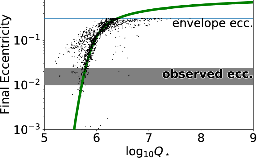
Figure 1: Example of the Bayesian analysis applied to a single binary in our sample (NGC 188 binary PKM 4618). Green line: final eccentricity as a function of $Q_{\star}^{\prime}$ (assumed constant), ignoring observational uncertainties (assuming median values for all binary properties). Cloud of black points: MCMC samples of $\log_{10}Q_{\star}^{\prime}(P_{tide}=5\,d)$ accounting for all observational uncertainties and variable $Q_{\star}^{\prime}$.

Fig. 1 shows this method applied to a single binary (NGC 188 binary PKM 4618). The horizontal line near the top is the value of the period-eccentricity envelope evaluated at the orbital period of the binary. The grey area slightly below the middle shows the measured eccentricity of the system (1-sigma error bar), and the green line shows the final eccentricity of a binary containing the same stars as PKM 4618 (median parameters), if it started with an initial eccentricity of 0.8, and with an orbital period that evolves to the observed orbital period at the present age. Finally, the points are the Bayesian analysis samples, following the posterior distribution defined above. At low $Q_{\star}^{\prime}$ (high dissipation), no matter the initial eccentricity, the system is circularized before its present age, so no initial conditions exist that would evolve to the observed present orbit. At high $Q_{\star}^{\prime}$, a system of identical stars starting with high initial eccentricity would end up above the envelope, also inconsistent with observations.

2.4 Sampling and Convergence Diagnostics

In order to carry out the Bayesian analysis, using the likelihood function defined above, we rely on the emcee python package (Foreman-Mackey et al., 2013) based on the Goodman & Weare (2010) affine invariant sampling algorithm. At each MCMC step, the algorithm simultaneously advances a collection of multiple individual, not independent, chains, called walkers. We chose to use 64 walkers. The combined samples of all walkers obey all standard requirements of the MCMC algorithm, and hence as the number of samples increases the distribution of samples approaches the desired posterior.

We initialize the sampler with 64 initial positions chosen to be over-dispersed compared to the posterior. To generate these samples, we draw uniform random values between 0 and 1, apply the prior transform described above, run the orbital evolution to the present system age, and keep any samples that land below the period-eccentricity envelope. For samples that land above the envelope, we re-draw new independent values and repeat the process. The reason to avoid starting walkers in configurations that evolve to above the period-eccentricity envelope is that per our definition, the likelihood function there is exactly zero, so the acceptance probability for most proposed updates for such values is undefined.

One of the key issue any MCMC analysis needs to address is demonstrating that sampling has run long enough for the samples to follow the target posterior distribution. One common approach is to split sampling in two stages. First, an initial burn-in period is introduced, during which samples potentially started from very low likelihood regions find their way to higher likelihoods. These initial samples have the potential to bias any estimates of quantities of interest away from their true values for finite length chains, so the usual practice is to discard those from further analysis. After the burn-in period, samples are used to extract estimates of the desired quantities. In addition to the need to determine the burn-in cut off, the often highly correlated nature of MCMC chains presents a challenge to estimating uncertainties in reported quantities.

In this effort we wish to find confidence intervals for the value of $\log_{10}Q_{\star}^{\prime}$ as a function of tidal period, which implies measuring quantiles of its distribution. Raftery & Lewis (1991) provide a procedure to find a required burn-in period, and a formalism for calculating the variance of quantile estimates. We follow their method, but adapt it to the peculiar emcee sampling involving many walkers. Appendix B gives the details of how the method was adapted to this analysis. As a result of following the procedure of Appendix B, we get an estimate of the burn-in period (the number of samples to be discarded before our estimates of the 2.3%, 15.9%, 84.1%, 97.7% quantiles of the posterior distribution have converged) and an estimate of the uncertainty of the CDF at each of those quantiles using only steps after the burn-in period.

3 Input Data

In order to carry out the analysis described in Section 2, we need observational constraints of the age, metallicity, extinction, and distance to the three open clusters targeted by this study, as well as RV and photometric measurements for the short period SB1 systems contained in these clusters.

The cluster properties assumed (along with references) are presented in Table 2. For each cluster, we analyze single line spectroscopic binaries flagged as open cluster members with orbital periods shorter than 50 days. The binaries which meet these criteria but for which no circularization analysis is reported here, along with the reason for their exclusion, are described separately for each cluster below.

Table 2: The observationally constrained properties of the three open clusters analyzed.

M 35
Age $\Big{(}\mu_{t,cl}\pm\sigma_{t,cl}\Big{)}$	$150\pm 30\,Myr^{f}$
$\left[\frac{Fe}{H}\right]$ $\Big{(}\mu_{\left[\frac{Fe}{H}\right],cl}\pm\sigma_{\left[\frac{Fe}{H}\right],cl}\Big{)}$	$-0.18\pm 0.03^{i,j}$
Extinction ($E(B-V)$)	$0.2^{h}$
Distance modulus	$9.6^{g}$
NGC 6819
Age $\Big{(}\mu_{t,cl}\pm\sigma_{t,cl}\Big{)}$	$2.4\pm 0.3\,Gyr^{a}$
$\left[\frac{Fe}{H}\right]$ $\Big{(}\mu_{\left[\frac{Fe}{H}\right],cl}\pm\sigma_{\left[\frac{Fe}{H}\right],cl}\Big{)}$	$0.09\pm 0.03^{b}$
$\mathrm{(B-V)}$	$0.15^{b}$
Distance modulus	$11.85^{a}$
NGC 188
Age $\Big{(}\mu_{t,cl}\pm\sigma_{t,cl}\Big{)}$	$7.0\pm 0.5\,Gyr^{c}$
$\left[\frac{Fe}{H}\right]$ $\Big{(}\mu_{\left[\frac{Fe}{H}\right],cl}\pm\sigma_{\left[\frac{Fe}{H}\right],cl}\Big{)}$	$0.10\pm 0.05^{e}$
Extinction ($E(B-V)$)	$0.08^{c}$
Distance modulus	$11.3^{c,d}$

• Basu et al. (2011)

• Bragaglia et al. (2001)

• Sarajedini et al. (1999)

• Gao (2018)

• Worthey & Jowett (2003)

• Meibom et al. (2009)

• Abdelaziz et al. (2022)

• Kalirai et al. (2003)

• Netopil et al. (2016)

• Barrado y Navascués et al. (2001)

3.1 M 35

We use the Leiner et al. (2015) $V$ and $B-V$ photometry and RV measurements for SB1s in M 35. We select only systems with orbital period less than 50 days. The authors collected photometry from two sources: observations by T. von Hippel using the Burrell Schmidt telescope at KPNO and observations by Deliyannis using the WIYN 0.9m telescope (no cite-able sources were given and we were unable to locate such ourselves). The second source is deemed higher precision by the authors, and Geller et al. (2010) quote that the $V$ magnitude differences between the two sources is approximately Gaussian with $\sigma=0.06\,mag$. Based on this information, we model the photometry likelihood function ($f_{phot}$ from Section 2.3) as a product of a Gaussian distribution of the $V$ magnitude with $\sigma=0.06/0.03$, and an independent Gaussian distribution of the $B$ magnitude with $\sigma=0.08/0.04$ if the photometry for the particular binary came from the low/high precision source. In addition, since we only use SB1 systems, only the spectrum of the brighter star in the binary was detectable. We conservatively require that the difference in $V$ magnitudes between the primary and the secondary star in the system should be at least 1, otherwise presumably this would have been a double lined binary.

We use the values given in Table 5 of Leiner et al. (2015) for the orbital periods and the parameters for the RV semi-amplitude ($\kappa$) and eccentricity ($\epsilon$) distributions. As described in Section 2.3 we approximate $\kappa$ by a Rice distribution with shape parameter given by the ratio of the measured value to the uncertainty and scale given by the uncertainty from Leiner et al. (2015) Table 5, and $\epsilon$ is assumed Gaussian with the given mean and $\sigma$.

We also use the Leiner et al. (2015) binaries deemed to be members of M 35 to construct a period-eccentricity envelope (see Fig. 2):

$$e_{env}(P_{orb})=0.05+\max\left[0,1.356\log_{10}\left(\frac{P_{orb}}{8\,days})\right)\right]$$ (16)

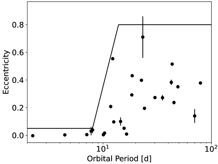
Figure 2: Period eccentricity envelope (black line) assumed for M 35. The circles show all binaries flagged as members by Leiner et al. (2015). At large periods we show the envelope saturating at $e_{env}=0.8$ because our orbital evolution with $e_{0}=0.8$. Hence, the highest eccentricity our model is capable of reproducing is $e=0.8$

Two SB1 systems with orbital periods less than 50 days were not included in this analysis: WOCS 49043 and WOCS 15012, because for rare cases of initial conditions, calculating their orbital evolution encountered numerical instabilities at very young ages. We worried that simply rejecting such samples could in theory bias the results, as it is in effect imposing another, ill-defined, prior. Work is on-going on a follow-up article that will expand the analysis presented here to many more clusters, and include double-lined binaries in addition to SB1s, where we hope to resolve these issues and include these systems. The observational data for all M 35 binaries used by this study is presented in Table 3.

Table 3: Observationally determined properties of the M 35 binary systems used to constrain tidal dissipation.

WOCS	$\bm{P_{orb}}$	$\bm{e}$	$\bm{K_{RV}}$	V	B-V
54027	2.247	$-0.003\pm 0.004$	$46.13\pm 0.21$	15.95	1.02
16016	7.089	$0.005\pm 0.006$	$30.18\pm 0.15$	14.25	0.63
23043	7.761	$0.030\pm 0.030$	$10.00\pm 0.40$	14.75	0.82
54054	8.013	$0.039\pm 0.024$	$8.26\pm 0.21$	15.00	0.78
35045	10.077	$0.004\pm 0.005$	$49.86\pm 0.24$	14.50	0.82
40015	10.330	$0.016\pm 0.007$	$40.50\pm 0.30$	15.34	0.84
33054	11.771	$0.208\pm 0.013$	$45.50\pm 0.60$	14.88	0.73
59018	18.427	$0.292\pm 0.010$	$37.40\pm 0.40$	16.10	1.10
14025	22.619	$0.398\pm 0.010$	$17.47\pm 0.21$	14.32	0.64
24023	30.134	$0.273\pm 0.004$	$28.19\pm 0.22$	15.02	0.85
9016	41.201	$0.372\pm 0.013$	$16.23\pm 0.22$	13.55	0.63
37029	45.121	$0.237\pm 0.013$	$22.70\pm 0.30$	15.14	0.87
20016	49.073	$0.351\pm 0.013$	$16.81\pm 0.18$	14.86	0.77

3.2 NGC 6819

We use the orbital period, RV semi-amplitude, and eccentricity for NGC 6819 SB1 systems reported in Table 5 of Milliman et al. (2014), together with the $V$ and $I$ photometry of Yang et al. (2013) as reported in table 2 of Milliman et al. (2014). Milliman et al. (2014) also provide error estimates for the photometric measurements by comparing to earlier photometry collected by Sarrazine et al. (2003), estimating $\sigma_{V}=0.036\,mag$ and $\sigma_{I}=0.039\,mag$.

Similarly to M 35 we define a period-eccentricity envelope for NGC 6819, shown in Fig. 3:

$$e_{env}(P_{orb})=0.05+\max\left[0,1.340\log_{10}\left(\frac{P_{orb}}{8\,days})\right)\right]$$ (17)

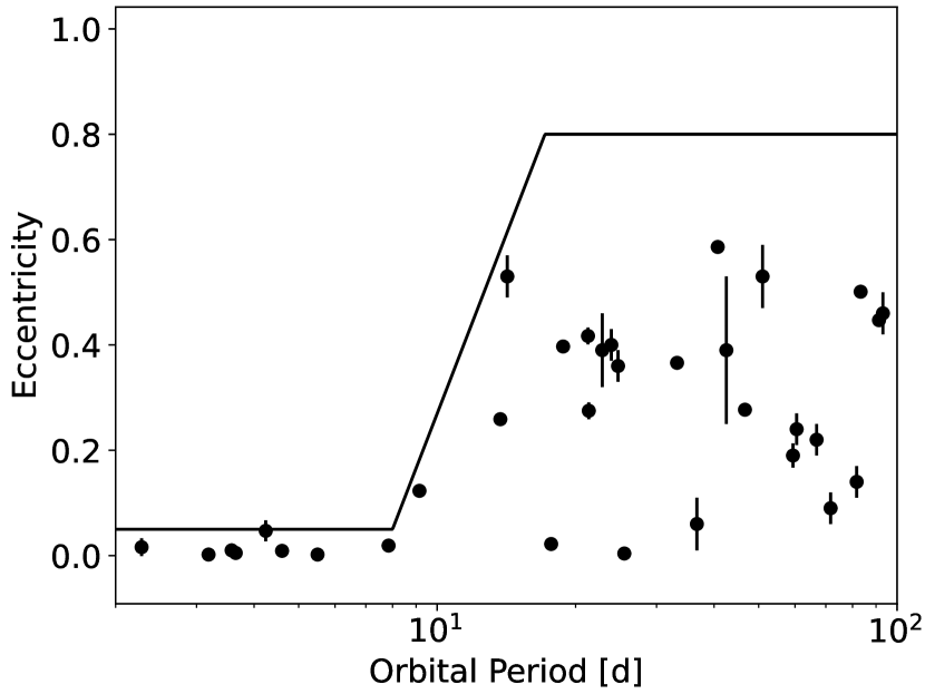
Figure 3: Same as Fig. 2 but for NGC 6819. Binary data from Milliman et al. (2014).

In the case of NGC 6819, a significant number of binaries with $P_{orb}<50\,d$ were excluded from this analysis (listed below).

WOCS 57004: We found that the posterior likelihood (Eq. 15) for this system is non-negligible only for a very narrow range of parameters. This is mostly due to the fact that the observed eccentricity ($e=0.123\pm 0.006$) is very close to the envelope eccentricity of Eq. 17 at the orbital period of this system ($e_{env}=0.128$). While in principle this is good news, since it implies this binary will provide very stringent constraints on tidal dissipation, it also makes the inferred posterior very sensitive to the exact shape of the distribution assumed for the present day eccentricity. Extracting reliable results for this binary thus requires an in-depth study of the impact of different assumed $\epsilon(e)$ and period-eccentricity envelopes, which will be addressed in an upcoming study that will expand the analysis presented here to a significantly larger sample of binaries.

Binaries with WOCS identifiers: 33002, 3002, 25004, 31004, 21007, 24012, 39013, 8012, 26007: The primary mass in these systems is near or above the threshold where the surface convective zone becomes negligible. Most theoretical models predict that such stars will be subject to very different tidal dissipation compared to stars with significant surface convective zones. Since our goal is to construct a combined constraint based on all binaries in a cluster we exclude these systems in order to avoid erroneously combining measurements of potentially different physical quantities.

The observational data for all NGC 6819 binaries used by this study is presented in Table 4.

Table 4: Observationally determined properties of the NGC 6819 binary systems used to constrain tidal dissipation.

WOCS	$\bm{P_{orb}}$	$\bm{e}$	$\bm{K_{RV}}$	V	V-I
49002	1.616	$0.022\pm 0.020$	$53.70\pm 1.20$	16.23	0.80
66004	2.278	$0.016\pm 0.017$	$38.60\pm 0.70$	16.10	0.80
13001	4.241	$0.047\pm 0.020$	$55.10\pm 1.00$	15.87	0.85
60006	7.843	$0.019\pm 0.011$	$33.14\pm 0.22$	16.11	0.83
46013	14.211	$0.530\pm 0.040$	$10.80\pm 0.50$	15.95	0.76
59003	21.368	$0.275\pm 0.016$	$31.60\pm 0.40$	16.40	0.83
35020	24.737	$0.360\pm 0.030$	$12.40\pm 0.50$	15.80	0.77
53003	42.540	$0.390\pm 0.140$	$5.40\pm 1.00$	16.29	0.81

3.3 NGC 188

Orbital period, RV semi-amplitude, and eccentricity information for NGC 188 binaries used in this analysis were taken from Table 2 of Geller et al. (2009). Photometric measurements in $u^{\prime}$, $g^{\prime}$, $r^{\prime}$, $i^{\prime}$, and $z^{\prime}$ bands were taken from Fornal et al. (2007) and $U$, $B$, $V$, $R$, and $I$ measurements were taken from Stetson et al. (2004).

Like for the other clusters, we define a period-eccentricity envelope based on the observed binary orbits (see Fig. 4):

$$e_{env}(P_{orb})=\max\left[0,0.316\log_{10}\left(\frac{P_{orb}}{3\,days})\right)\right]$$ (18)

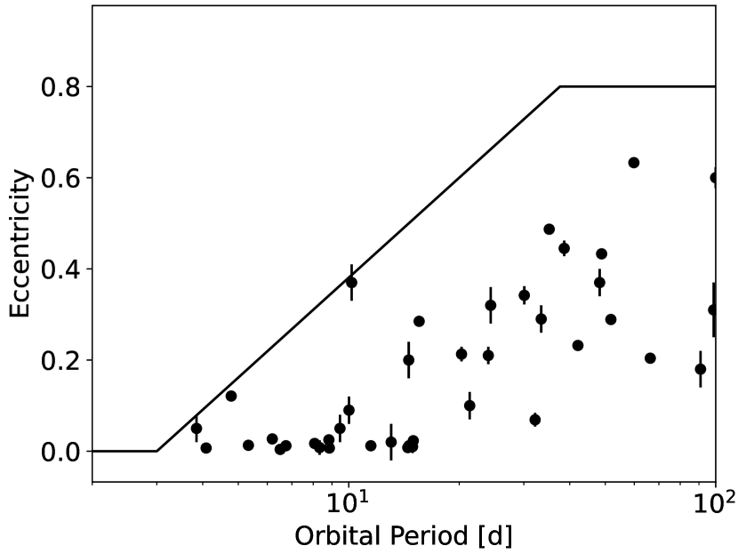
Figure 4: Same as Fig. 2 but for NGC 188. Binary data from Geller et al. (2009).

Note that the period eccentricity envelope we assumed for NGC 188 is pushed to significantly higher eccentricities by just two systems, with PKM IDs 5078 ($P_{orb}=4.78303\pm 0.00012$, $e=0.121\pm 0.006$) and 4904 ($P_{orb}=10.185\pm 0.003$, $e=0.37\pm 0.04$). There is a clear pile-up of circular systems for orbital periods all the way to 14 days or so, indicating these systems are likely outliers. There is very little doubt either binary is a member of the cluster with both their systemic radial velocity and proper motion closely matching that of the cluster. One possibility Geller et al. (2009) point out is that tertiary companions are not infrequent for short period binary systems of solar type stars. As a result, these systems are potential exceptions to the envelope for binaries shaped only by tides. Regardless, we choose to define the envelope in a way that accommodates these systems, since per our method that is the conservative assumption, increasing the uncertainty in the inferred tidal dissipation parameters, while still including the values that would be inferred with a lower period-eccentricity envelope.

Of the Geller et al. (2009) SB1 binaries with $P_{orb}<50\,d$ we exclude 2 systems:

PKM 4710: This system is flagged as a cluster member in Geller et al. (2009) but at the same time the same authors quote its radial velocity membership probability to be 1%, though it appears to be a member based on its proper motion. To be safe, we exclude the binary from our analysis.

PKM 4999: The distribution of the secondary star’s mass in this system extends to very small values (as low as $\sim 0.1M_{\odot}$). Thus, there is a reasonable chance that this is a fully convective star. At least some tidal dissipation models predict very different dissipation for fully convective stars vs stars with a significant radiative core. Since tidal circularization is dominated by the dissipation in the secondary star, we don’t necessarily expect the dissipation measured for PKM 4999 to be similar to all other binaries analyzed in this effort so we exclude the system from the analysis.

Table 5 presents the observational data for all NGC 188 binaries included in this study.

Table 5: Observationally determined properties of the NGC 188 binary systems used to constrain tidal dissipation.

PKM	$\bm{P_{orb}}$	$\bm{e}$	$\bm{K_{RV}}$	U	B	V	R	I	u	g	r	i	z
5052	3.847	$0.050\pm 0.030$	$8.80\pm 0.30$	16.82	16.63	15.92	15.47	15.08	17.77	16.30	15.75	15.58	15.60
4618	8.073	$0.017\pm 0.007$	$55.10\pm 0.40$	16.72	16.48	15.77	15.33	14.90	17.57	16.13	15.57	15.36	15.27
5015	8.329	$0.008\pm 0.016$	$45.60\pm 0.70$	17.20	16.83	16.03	15.55	15.10	18.05	16.37	15.76	15.55	15.40
6171	8.828	$0.025\pm 0.011$	$35.90\pm 0.40$	17.32	17.05	16.31	15.83	15.46	—	—	—	—	—
5463	9.465	$0.050\pm 0.030$	$6.24\pm 0.22$	15.80	15.64	14.98	14.58	14.20	16.61	15.29	14.83	14.66	14.55
5601	10.014	$0.090\pm 0.030$	$5.67\pm 0.10$	16.45	16.28	15.60	15.16	14.79	—	—	—	—	—
4904	10.185	$0.370\pm 0.040$	$11.20\pm 0.50$	16.91	16.66	15.93	15.49	15.07	—	—	—	—	—
4289	11.488	$0.012\pm 0.010$	$40.80\pm 0.30$	16.94	16.24	15.30	14.77	14.20	—	—	—	—	—
5738	13.049	$0.020\pm 0.040$	$5.92\pm 0.20$	16.10	15.99	15.31	14.91	14.55	16.97	15.62	15.16	14.98	14.86
6292	14.599	$0.012\pm 0.007$	$30.99\pm 0.19$	—	16.21	15.52	—	—	—	—	—	—	—
4965	14.922	$0.010\pm 0.014$	$17.38\pm 0.20$	16.14	15.97	15.28	14.86	14.45	16.80	15.35	14.83	14.65	14.60
5797	14.991	$0.023\pm 0.011$	$19.53\pm 0.23$	16.76	16.54	15.85	15.41	15.03	—	—	—	—	—
5647	15.553	$0.285\pm 0.011$	$45.50\pm 0.70$	17.00	16.74	16.00	15.54	15.13	17.82	16.36	15.80	15.60	15.55
880	20.292	$0.213\pm 0.016$	$15.40\pm 0.30$	—	16.07	15.38	—	—	—	—	—	—	—
4080	32.197	$0.069\pm 0.015$	$20.70\pm 0.30$	16.38	16.20	15.52	15.11	14.73	—	—	—	—	—
5040	33.455	$0.290\pm 0.030$	$6.91\pm 0.24$	15.86	15.68	15.01	14.60	14.23	16.72	15.31	14.82	14.65	14.59
4673	48.270	$0.370\pm 0.030$	$8.40\pm 0.30$	15.88	15.60	14.88	14.45	14.05	16.72	15.21	14.68	14.50	14.41

4 Results

4.1 System-by-System Constraints

For all binaries included in this study, we generated MCMC samples following the procedure described in Sec. 2. For each MCMC sample generated, we evaluate the tidal dissipation model (Eq. 12) at each tidal period to produce samples of $\log_{10}Q_{\star}^{\prime}$ as a function of $P_{tide}$. We then convolve these samples with an Epanechnikov (quadratic) kernel of width 0.2 to approximate the posterior probability density function of $\log_{10}Q_{\star}^{\prime}$ at each tidal period. Figures 5 — 7 display the decimal logarithm of the inferred probability density for each system scaled such that it has a maximum value of 1 (the color scale spans 3 orders of magnitude in likelihood). The vertical black line marks the orbital period of the system, and the 4 black curves from bottom to top show the 1- and 2-sigma equivalent quantiles ($\log_{10}Q_{\star}^{\prime}$ where the cumulative distribution is 2.3%, 15.9%, 84.1%, and 97.7% respectively).

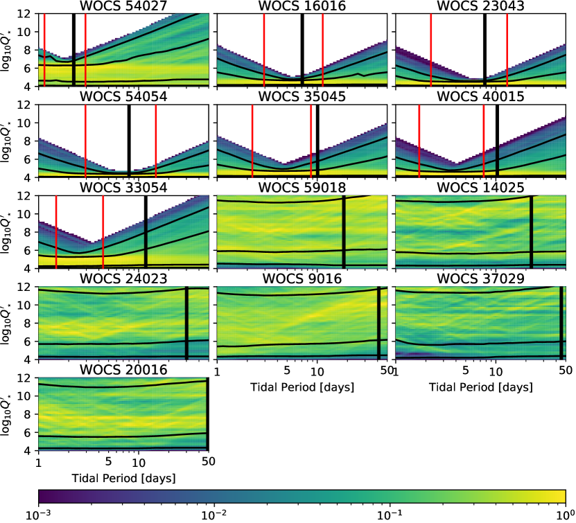
Figure 5: Constraints for $log_{10}Q_{\star}^{\prime}$ obtained for the individual M 35 binaries. The color scale in each plot shows the posterior probability density function ($\log_{10}$ scale) of the tidal dissipation parameter as a function of tidal period. The vertical red lines demarcate the range of tidal periods where the constraints are dominated by observations rather than model assumptions and priors (see text). The thin black curves show 2.3%, 15.9%, 84.1%, and 97.7% quantiles respectively.

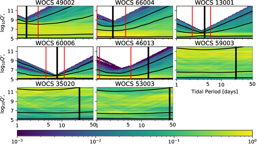
Figure 6: Same as Fig. 5 but for the NGC 6819 binaries analyzed.

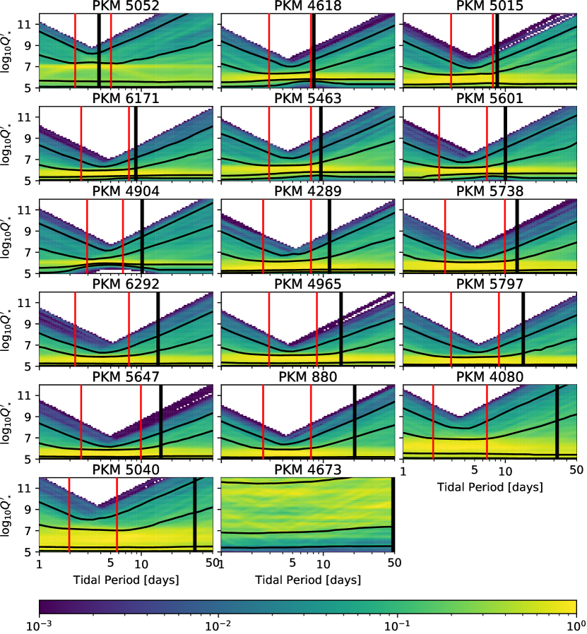
Figure 7: Same as Fig. 5 but for the NGC 188 binaries analyzed.

The v-shaped appearance of Fig. 5 — 7 upper quantiles and the period of the most stringent upper limit (bottom of the V) for each system can intuitively be understood to be produced by the period-eccentricity envelope. Per our method, the highest value $Q_{\star}^{\prime}$ can take is such that the system should land on the period-eccentricity envelope. For orbital periods where significant circularization is expected (envelope is significantly below the starting value of $e=0.8$) there is a narrow range of tidal terms that dominate the final stages of the circularization.

At short orbital periods, when the envelope only allows for very close to circular orbits, the limiting stage of the circularization process is at the very end, when the eccentricity is small. In that case, the higher frequency tidal potential terms have very small amplitudes, so they are unable to support a spin-orbit lock at the corresponding frequency. As a result, the stellar spin period is very close to the orbital period (star spins pseudo-synchronously). The dominant tidal perturbation in those cases has a frequency equal to the orbital period, because in a reference frame rotating with the star, the companion moves closer and further away with each orbit but stays in approximately the same direction. Hence, this is the term that is most constrained by our analysis.

At longer orbital periods, $Q_{\star}^{\prime}$ values at the highest quantiles of the distribution place the system on the envelope, which has significant eccentricity, and can sustain higher order spin-orbit locks: $2\Omega_{\star}=k\Omega_{orb}$ for k > 2. Since stars get spun-up as they contract to the main sequence to rates far exceeding the orbital period, their spins generally get stuck at the highest $k$ for which a spin-orbit lock can be maintained for a given orbit. The effect of this picture is that the dominant tidal wave for longer orbital period systems at the weakest allowed tidal dissipation (largest value of $Q_{\star}^{\prime}$) has a higher frequency (shorter period) than the orbit, and hence the tightest upper limit on $Q_{\star}^{\prime}$ lies at a fraction of the orbital period.

Moving sufficiently away from the tidal periods where the dissipation is best constrained, we see that the highest quantile curve has a slope $\frac{d\log Q_{\star}^{\prime}}{dP_{tide}}\approx 5$, matching the prior limits we placed on the powerlaw index of the assumed tidal dissipation model (Eq. 12). Thus, far away from the best constrained period range, it is our prior, rather than data, that dominates the constraints. In each plot in Fig. 5 — 7, the region between the two vertical red lines provides a rough idea of the range of periods where the constraints are driven by the observational data, and hence is informative for understanding tidal dissipation. The exact locations were defined by requiring that the 97.7th percentile of the distribution of $log_{10}Q_{\star}^{\prime}$ does not exceed its minimum by more than 0.7 dex. Only samples after the empirically determined burn-in period (see Sec. 2.4) were used when building these distributions. We thus choose the largest burn-in period across all quantiles and tidal periods between the red lines in the plots.

Additionally, as expected, for all systems where the observed present day eccentricity is consistent with circular orbit, the 2.3% quantile is determined by the lower limit we assume in Eq. 12. For circularized systems our method only gives an upper limit to $Q_{\star}^{\prime}$. Only systems for which observations can confidently exclude circular orbits produce a lower limit on $Q_{\star}^{\prime}$ (upper limit on the dissipation).

In particular, none of the M 35 binaries constrains $Q_{\star}^{\prime}$ from below. This is because, as Fig. 2 shows, the orbits of all binaries in M 35 out to orbital periods of 10 d are indistinguishable from circular, and all longer period binaries are in the regime where tides have not significantly impacted the orbit. The former as already discussed give only upper limit to $Q_{\star}^{\prime}$ (lower limit on the dissipation) and the latter produce no useful constraints (e.g. the last 6 panels of Fig. 5).

Tables 6 — 8 list the 2.3%, 15.9%, 84.1%, and 97.7% quantiles of $\log_{10}Q_{\star}^{\prime}$ for each system at the tidal period where the 97.7-th quantile is the smallest (i.e. the bottom of the V). The table also compares these individual constraints with the combined constraint (see Sec. 4.2). We also provide in machine readable format the quantile curves shown in each of the plots (see Sec. Data Availability).

One result immediately evident from Figures 5 — 7 is that explaining the observed period-eccentricity distribution of the young M 35 binaries requires significantly more dissipation (by a factor of approximately 30) than explaining the much older NGC 6819 and NGC 188 (note different lower limits of the y-axes in the figures). The constraints based on all M 35 binaries are consistent with each other, and many binaries require $\log_{10}Q_{\star}^{\prime}<5$. In contrast binaries in NGC 6819 and NGC 188 produce consistent constraints within and between the two clusters, with several requiring values of $\log_{10}Q_{\star}^{\prime}\gtrsim 5.5$.

Figures 8 — 10 show the estimate of the required burn-in period for the sampling to reach the equilibrium distribution for a given quantile of $Q_{\star}^{\prime}(P_{tide})$ (lines), calculated per Section 2.4. The black area of the plots show the total number of samples actually generated for each system. Figures 11 — 13 show the uncertainty (standard deviation) of the fraction of the posterior distribution below each of the estimated quantiles based on samples after the corresponding burn-in period. In each plot, the red-lines again delineate the range of tidal periods where the dissipation is reliably constrained by observations.

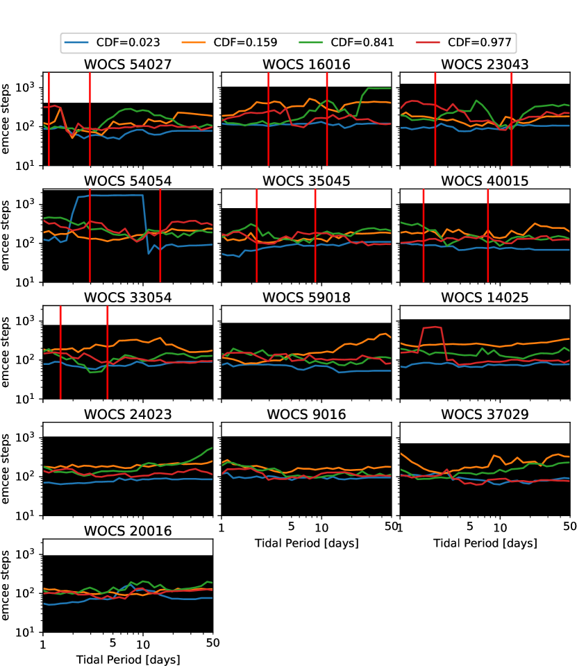
Figure 8: Diagnostics for the convergence of the MCMC chains. Each curve shows the estimate of the number of emcee steps required for subsequent samples to have the equilibrium probability of lying below or above a particular quantile (color lines). Those were used as the burn-in period when estimating posteriors (see text). The black area of each plot shows the total number of steps generated during the sampling of this system. The vertical red lines match those in Fig. 5, showing the range of periods where the constraints are driven by the data as opposed to priors.

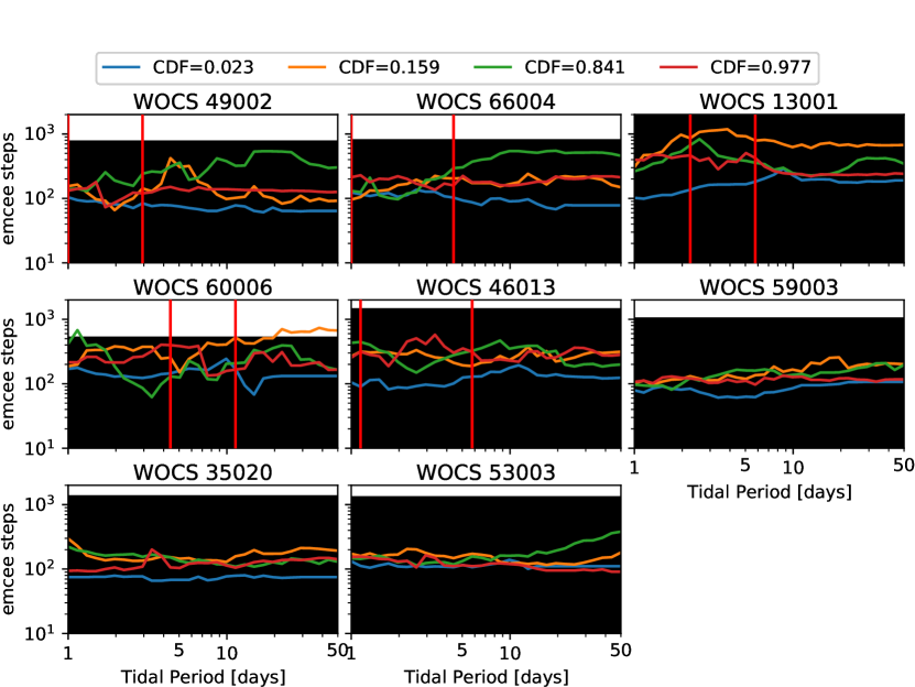
Figure 9: Same as Fig. 8 but for the NGC 6819 binaries analyzed.

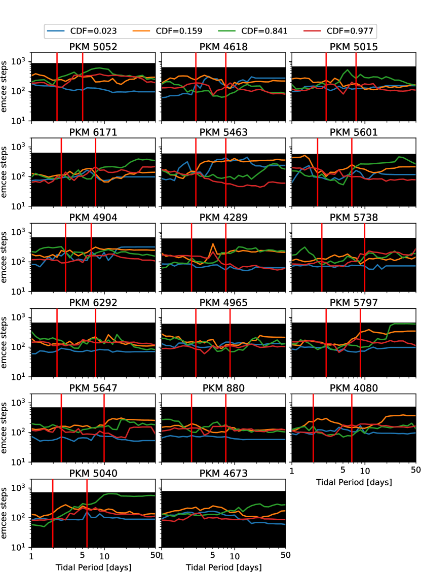
Figure 10: Same as Fig. 8 but for the NGC 188 binaries analyzed.

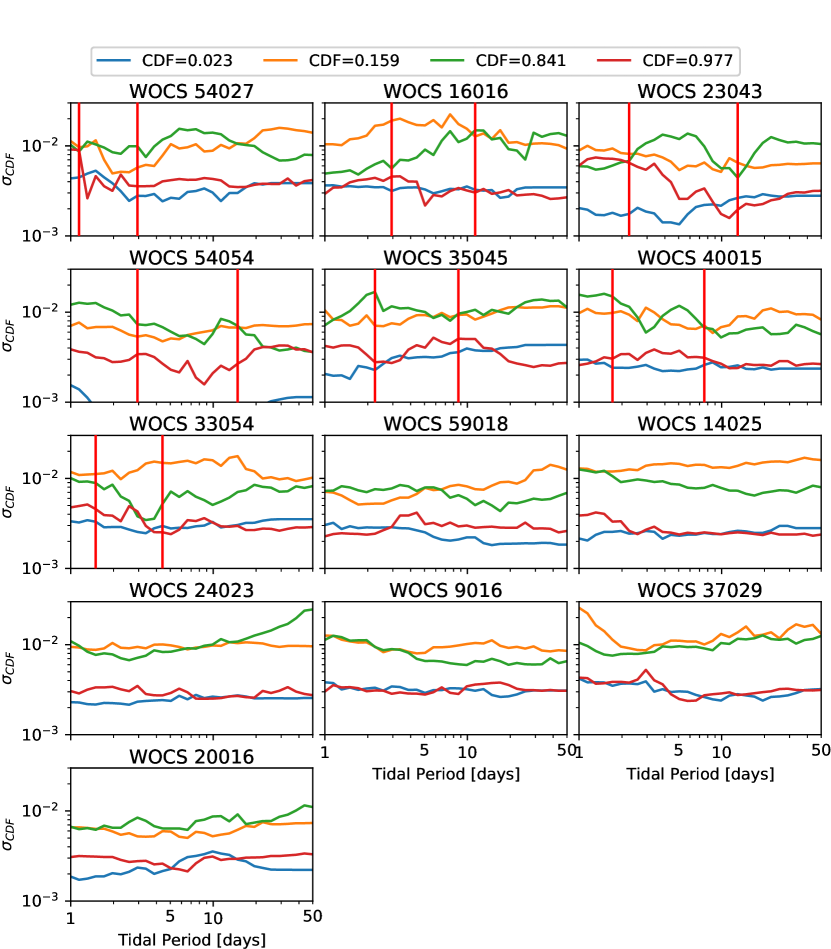
Figure 11: The estimated uncertainty in the fraction of samples below each of the 4 target quantiles for the M 35 binaries analyzed. Each curve shows the estimate of the standard deviation of the cumulative distribution evaluated at a particular quantile (color lines). The red lines match those in Fig. 5.

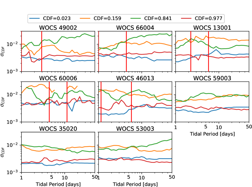
Figure 12: Same as Fig. 11 but for the NGC 6819 binaries analyzed.

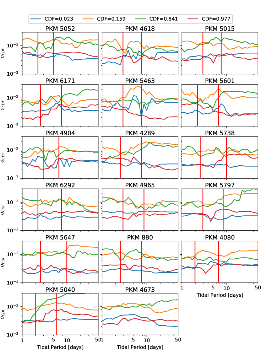
Figure 13: Same as Fig. 11 but for the NGC 188 binaries analyzed.

We see from Fig. 8 — 10 that all chains contain sufficient samples to ensure that the 2.3%, 15.9%, 84.1%, and 97.7% quantiles of $\log_{10}Q_{\star}^{\prime}$ have converged to their equilibrium values for all tidal periods this analysis is sensitive to (between the red vertical lines). Furthermore, Fig. 11 — 13 show that the estimated quantiles correspond to the targeted CDF values to better than 10% relative precision. For example, for the M 35 binary WOCS 40015, Fig. 8 shows that about 200 steps are required for all four diagnostic quantiles to converge, while we generated more than 1000 samples for that system. Similarly, Fig. 11 shows that for the diagnostic quantiles, in the well-constrained range of tidal periods, the fraction of samples below the corresponding estimated value is $(2.3\pm 0.3)\%$, $(16\pm 1)\%$, $(84\pm 1)\%$, and $97.7\pm 0.4)\%$ respectively for the same binary.

4.2 Combined Constraints

In order to find constraints that explain all binaries simultaneously, we construct a combined probability density for the tidal dissipation in M 35 by multiplying the posteriors of all 13 systems together, but only in the range we identify as data dominated (i.e. between the red lines in Fig. 5 — 7). The result is shown in Fig. 14. Note that the y axis has been restricted to $4<\log_{10}Q_{\star}^{\prime}<6$, since higher values have negligible likelihood.

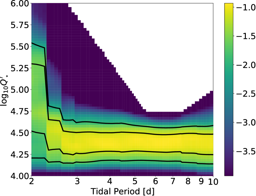
Figure 14: Combined constraint from all M 35 binaries constructed by multiplying together the individual constraints of Fig. 5 only in the regions between the two red lines for each system. The sudden jumps in period are due to contributions from various constraints sharply turning on and off at these period boundaries.

Similarly, we combine all constraints of the 25 binaries in NGC 6819 and NGC 188 in Fig. 15. In this case however, we constructed two distribution, one with and one without the NGC 188 binary PKM 4904. As can be seen in the figure, the two constraints are virtually identical. As noted in 3.3, PKM 5078 and PKM 4904 are in clearly non-circular orbits but have orbital periods well into the range where all other binaries in this cluster are circularized. As already discussed this could be an indication that tides are not the only mechanism shaping the orbits of these systems. PKM 5078 is a double line spectroscopic binary, and hence was already excluded from our analysis (postponed to future publications). It was important to check the possibility that PKM 4904 biases our results, but it does not appear to be the case. Note that these binaries still affect the results by shifting upward the period-eccentricity envelope used to define our posterior likelihood function for the MCMC analysis. As discussed in 3.3, raising (potentially erroneously) the envelope only broadens the inferred posterior, while still including the constraints that would be obtained had the envelope been defined without taking these binaries into account.

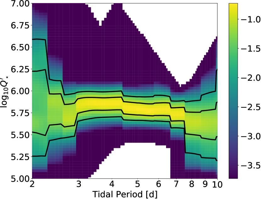
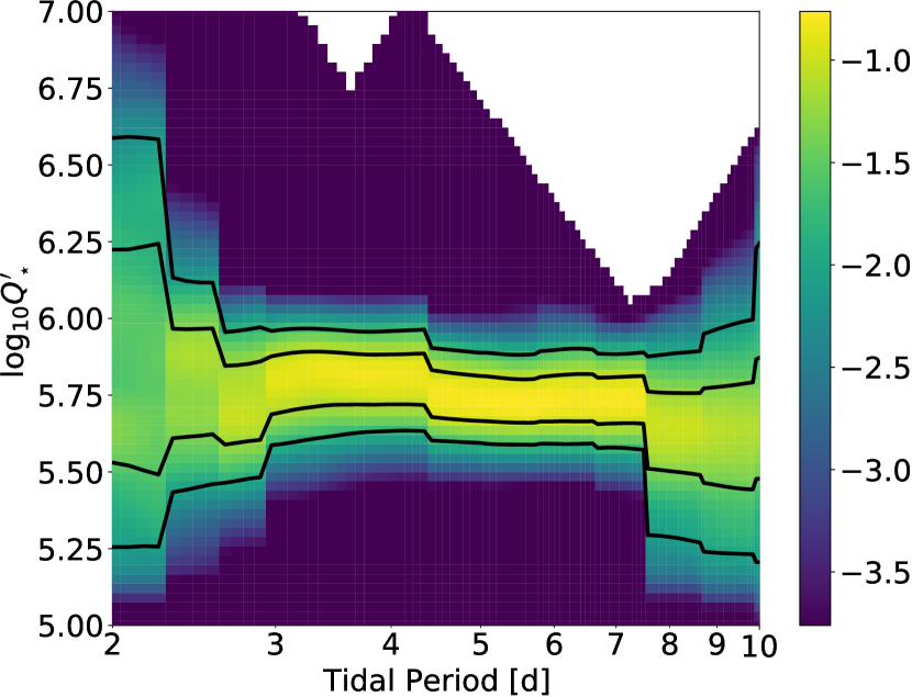
Figure 15: Top: Combined constraint from all NGC 6819 and NGC 188 binaries constructed by multiplying together the individual constraints of Fig. 5 only in the regions between the two red lines for each system. The sudden jumps in period are due to contributions from various constraints sharply turning on and off at these period boundaries. Bottom: same as top, but excluding NGC 188 binary PKM 4904 due to its potentially suspicious location in the period-eccentricity diagram of the cluster.

A reasonable question to ask of our combined constraints in Fig. 14 and 15 is whether they are able to simultaneously reproduce the observed and envelope eccentricities of all binaries included in this study. In other words, are the combined constraints in agreement with the individual constraints of Sec. 4.1. Fig. 16 compares the combined constraint from all M 35 binaries with the individual constraints used in building the combined one. The curves in the figure show the same 1- and 2-$\sigma$ equivalent quantiles shown in Fig. 14 and the error bars show the individual constraints for each system for the tidal period with the lowest 97.7-th percentile (the bottom of the V in the individual constraint plots). The thick/thin error bars shows the 1-/2-$\sigma$ equivalent quantiles for each system. The error bars that extend past the top of the plot correspond to long orbital period systems that provide no information on the dissipation beyond our priors, so their x coordinates are not meaningful.

Fig. 17 shows the same comparison between the individual constraints for NGC 6819 and NGC 188 binaries against the combined constraint from both clusters. We have introduced small offsets in tidal period for some of the points in order to avoid overlaps which make the plot difficult to read.

The combined constraints are also included in Tables 6 (M 35), 7 (NGC 6819), and 8 (NGC 188) along the corresponding individual constraints.

Table 6: Comparison of the combined constraints based on all M 35 binaries with the individual constraints for each binary at the tidal period where 97.7-th percentile of the $log_{10}Q_{\star}^{\prime}$ constraint is the smallest.

		Individual CDF-1				Combined CDF-1
WOCS	Ptide	2.3%	15.9%	84.1%	97.7%	84.1%	97.7%
54027	1.96	4.08	4.52	6.31	6.69	—	—
16016	5.78	4.03	4.19	4.66	4.78	4.49	4.57
23043	5.78	4.01	4.09	4.50	4.59	4.48	4.56
54054	6.61	4.00	4.06	4.38	4.47	4.48	4.56
35045	4.41	4.02	4.17	4.71	4.93	4.51	4.61
40015	3.37	4.02	4.15	4.62	4.79	4.51	4.62
33054	2.57	4.07	4.28	5.28	5.69	4.63	4.77
59018	5.05	4.48	5.83	11.27	13.05	4.50	4.58
14025	2.94	4.31	5.64	11.30	13.08	4.50	4.63
24023	4.41	4.31	5.72	11.25	12.94	4.50	4.59
9016	5.78	4.36	5.69	11.09	12.68	4.50	4.58
37029	3.85	4.21	5.70	11.34	13.00	4.50	4.61
20016	5.05	4.25	5.51	10.97	12.48	4.49	4.57

Table 7: Comparison of the combined constraints based on all NGC 6819 and NGC 188 binaries, except PKM 4904 with the individual constraints for each NGC 6819 binary at the tidal period where 97.7-th percentile of the $log_{10}Q_{\star}^{\prime}$ constraint is the smallest.

		Individual CDF-1				Combined CDF-1
WOCS	Ptide	2.3%	15.9%	84.1%	97.7%	2.3%	15.9%	84.1%	97.7%
49002	1.72	5.14	5.79	8.19	8.60	—	—	—	—
66004	1.96	5.06	5.39	6.74	7.66	5.26	5.51	6.23	6.59
13001	3.37	5.08	5.60	6.16	6.35	5.70	5.78	5.92	5.99
60006	6.61	5.02	5.21	5.72	5.85	5.58	5.66	5.81	5.89
46013	3.37	5.01	5.12	5.73	6.30	5.66	5.76	5.92	5.99
59003	2.94	5.39	6.52	11.40	12.63	5.68	5.77	5.93	5.99
35020	5.05	5.26	6.53	11.47	13.08	5.67	5.73	5.87	5.94
53003	3.85	5.28	6.34	11.18	12.87	5.71	5.78	5.93	6.00

Table 8: Comparison of the combined constraints based on all NGC 6819 and NGC 188 binaries, except PKM 4904 with the individual constraints for each NGC 188 binary at the tidal period where 97.7-th percentile of the $log_{10}Q_{\star}^{\prime}$ constraint is the smallest.

		Individual CDF-1				Combined CDF-1
PKM	Ptide	2.3%	15.9%	84.1%	97.7%	2.3%	15.9%	84.1%	97.7%
5052	3.37	5.10	5.62	7.42	8.22	5.70	5.78	5.93	5.99
4618	5.05	5.51	5.80	6.39	7.01	5.66	5.72	5.86	5.95
5015	4.41	5.05	5.39	6.27	6.86	5.70	5.78	5.93	5.99
6171	4.41	5.13	5.41	5.98	6.32	5.66	5.72	5.86	5.93
5463	5.05	5.35	5.76	6.45	7.11	5.70	5.78	5.93	6.00
5601	3.85	5.20	5.62	6.22	6.73	5.69	5.78	5.92	5.99
4904	4.41	5.81	5.97	6.46	7.15	5.70	5.78	5.92	5.99
4289	3.85	5.12	5.32	6.13	6.69	5.67	5.73	5.87	5.94
5738	5.78	5.03	5.25	6.07	6.46	5.58	5.66	5.81	5.88
6292	4.41	5.06	5.25	5.90	6.28	5.66	5.72	5.86	5.95
4965	5.05	5.04	5.29	6.05	6.40	5.58	5.66	5.81	5.89
5797	5.78	5.03	5.18	5.88	6.33	5.66	5.73	5.87	5.94
5647	5.05	5.04	5.22	5.88	6.15	5.70	5.78	5.92	5.99
880	3.85	5.02	5.17	5.91	6.38	5.68	5.77	5.92	5.99
4080	3.85	5.09	5.53	6.87	7.89	5.66	5.72	5.86	5.93
5040	3.37	5.08	5.43	7.09	8.04	5.48	5.60	5.85	5.96
4673	1.96	5.38	6.76	11.46	12.75	—	—	—	—

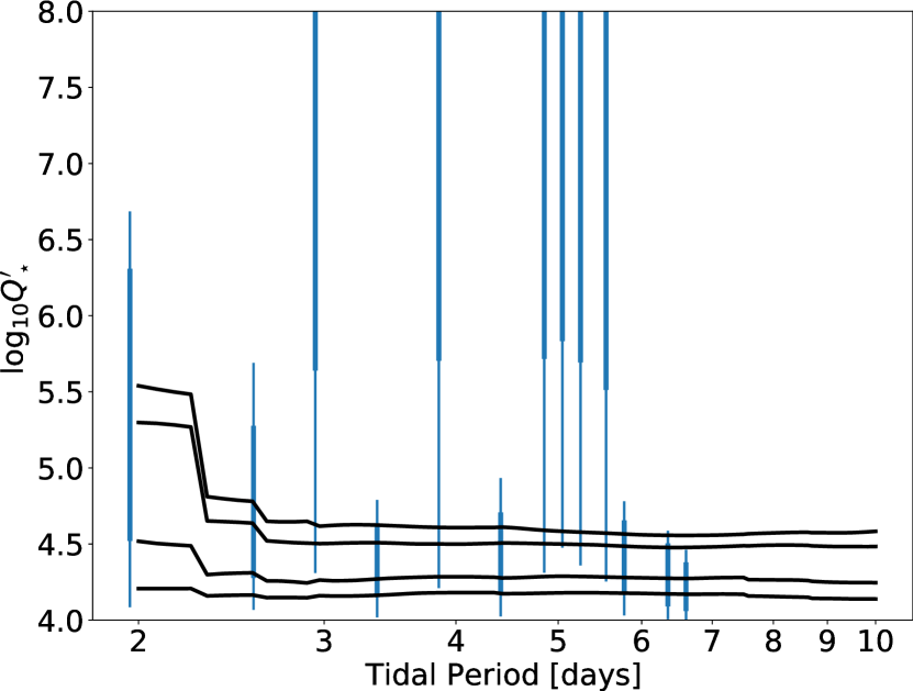
Figure 16: Comparison between the combined constraint of the tidal dissipation in M 35 stars to the individual constraints for each binary. The lines show the 2.3%, 15.9%, 84.1%, and 97.7% quantiles of the combined constraint (same as in Fig. 14), and the error bars show the same quantiles for individual systems at the tidal period where the dissipation is best constrained by observations. The thick part of the error bars spans from 15.9% to 84.1% of the posterior distribution and the thin error bar spans from 2.3%, to 97.7%. The x coordinate of error bars extending past the top of the plot is not well defined.

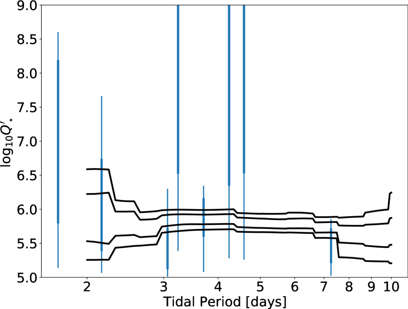
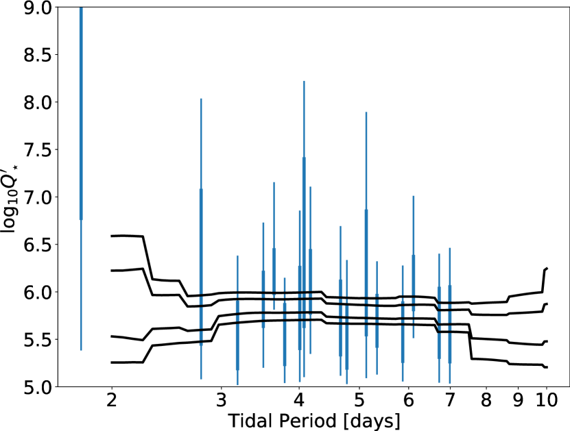
Figure 17: Comparison between the combined constraint of the tidal dissipation in NGC 6819 (top) and NGC 188 (bottom) stars to the individual constraints for each binary. The lines show the 2.3%, 15.9%, 84.1%, and 97.7% quantiles of the combined constraint for both clusters (same as in Fig. 15), and the error bars show the same quantiles for individual systems at the tidal period where the dissipation is best constrained by observations. The thick part of the error bars spans from 15.9% to 84.1% of the posterior distribution and the thin error bar spans from 2.3%, to 97.7%. The x coordinate of error bars extending past the top of the plot is not well defined.

As Fig. 16 and 17 demonstrate, the combined constraints are capable of reproducing the observed eccentricities for all binaries analyzed, as well as the period-eccentricity envelopes of all three clusters.

It is important to point out that the systems whose error bars stretch beyond the top of the plots are simply consistent with a very broad range of $Q_{\star}^{\prime}$ values, stretching over most of the prior range allowed with little preference if any for some values of $Q_{\star}^{\prime}$ over others. They should not be seen as preferring a higher value of $Q_{\star}^{\prime}$ than the combined constraint. This can be seen from the corresponding plots in Fig. 5 — 7. For example, the 6 systems that appear as outliers in Fig. 16 are the 6 longest period systems we analyzed for M 35 (those with WOCS identifiers 59018, 14025, 24023, 9016, 37029, 20016). As can be seen from 5, the $\log_{10}Q_{\star}^{\prime}$ samples are very close to uniformly distributed over the entire prior range, hence those systems provide no useful information. What is more, because the posteriors of these systems are so broad, their x coordinates in the figures above are ill defined. We only included those systems in the above plots for completeness.

Another conclusion that can be drawn from the combined constraints is that, at the tidal periods probed by this analysis ($2\,d<P_{tide}<10\,d$), there is no evidence for frequency dependence of $Q_{\star}^{\prime}$, even though our model explicitly allows for such a dependence. In fact, for sun-like stars on the main sequence (NGC 6819 and NGC 188), we place tight limits on the dissipation of $5.7<\log_{10}Q_{\star}^{\prime}<6$ for $3\,d<P_{tide}<7.5\,d$, implying that if $Q_{\star}^{\prime}\propto P_{tide}^{\alpha}$, then $|\alpha|<1$. Note that for models, like inertial wave coupling, predicting dramatic variations in $Q_{\star}^{\prime}$ with very small frequency changes, our result should be interpreted as constraints on the appropriately frequency-smoothed dissipation predicted by such models.

For the young stars of M 35, we only measure an upper limit to $Q_{\star}^{\prime}<4\times 10^{4}$ (lower limit on the dissipation), exceeding the dissipation of main-sequence stars by an order of magnitude (see Appendix C for a discussion of a small offset in the constraint that’s potentially introduced by ignoring the tidal evolution before 2 Myrs).

4.3 Assumptions and Caveats

The results presented in this article depend on several critical assumptions that bear consideration. First, our prescription for $Q_{\star}^{\prime}$ only includes frequency dependence, and we were able to split our sample into pre-MS dominated and MS dominated circularization, even though age dependent $Q_{\star}^{\prime}$ was not explicitly included in our modeling. However, depending on the exact dissipation mechanism, tidal frequency and age are far from the only factors that can affect the dissipation.

For instance, some dynamical tide models invoke tidal excitation of g-modes at the convective-radiative boundary, which then travel inward. (Barker & Ogilvie, 2010) find that if these waves achieve sufficient amplitude to break, $Q_{\star}^{\prime}\propto M_{\star}^{2}P_{tide}^{8/3}$. Wave breaking does not occur for weak tides, or if the star has a significant convective core ($M_{\star}\gtrsim 1.1M_{\odot}$) preventing waves from reaching the center. For weakly non-linear g-modes (non-breaking) (Essick & Weinberg, 2016) argue the non-linear excitation of (grand)daughter modes leads to $Q_{\star}^{\prime}\propto M_{\star}^{\prime 0.5}P_{tide}^{2.4}$, where $M_{\star}^{\prime}$ is the mass of the companion star. Finally, if g-modes remain linear, (Ma & Fuller, 2021) predict $Q_{\star}^{\prime}\propto M_{\star}^{-8/3}M_{\star}^{\prime}P_{tide}^{-13/3}$.

Another flavor of theoretical models invoke tidal excitation of inertial modes in the convective envelopes of stars, predicting dramatically increased dissipation for low mass stars if $P_{spin}<2P_{tide}$. Detecting this edge at the correct location would be a very strong indication of this mechanism dominating the dissipation. However, the angular momentum in the orbit is many orders of magnitude larger than the angular momentum in the spin. Consequently, tides cause stars to spin pseudo-synchronously on a much shorter timescale than they circularize the orbit. As a result, tidal circularization occurs almost exclusively with $P_{spin}<2P_{tide}$. Therefore, in the context of inertial mode coupling, our results should be interpreted as measuring a frequency smoothed version of the enhanced dissipation. Detecting inertial mode enhancement thus requires studying the effects of tides on other system properties, like tidal synchronization, or looking for signs of the expected mass and/or spin dependence of the predicted enhanced dissipation.

Allowing for additional degrees of freedom in the tidal dissipation prescription, like explicit age, spin, and amplitude dependence, will be investigated in further analyses we are currently pursuing, which include much larger samples of systems and hence have a chance of disentangling some of these dependencies.

The g-mode class of models also point out a second caveat in our analysis. We assumed that the tides couple to the surface convective zone of the stars in our sample, while these models predict coupling to the radiative core. This distinction makes a difference only if significant differential rotation can develop between the core and the envelope. If stars spin like solid bodies, one can always find an effective $Q_{\star}^{\prime}$ regardless of which zone couples to tides. Furthermore, since the orbit dominates the angular momentum budget of the system by many orders of magnitude, even large differential rotation will make little difference for the results presented here.

An additional critical assumption we make for this analysis is that tides are the only thing driving orbital evolution since early in the binary’s history. It is not uncommon to find triple and higher multiplicity systems, especially in clusters. If additional, undetected, companions are present in the binaries we analyze, they may excite the orbital eccentricity, causing us to under-estimate the amount of tidal dissipation present. In fact, we already mentioned this possibility as a possible explanation for the apparent outlier eccentricities of NGC 188 members PKM 4904 and PKM 5078, and even excluded these binaries when calculating the combined constraint in Fig. 15. One way such companions would show up in the data is through deviations of the RV measurements from strict periodicity (i.e. long term trends). None of the binaries included in our sample show evidence of this. Alternatively, we would expect binaries strongly affected by tertiary companions to produce anomalously large $Q_{\star}^{\prime}$ constraints, which again we see no evidence of. However, neither of these non-detections is a 100% guarantee that companions are not present.

Another potential caveat to our approach was recently pointed out by Zanazzi (2022) who find that the relatively small number of binary systems present in an individual cluster may miss important features of the period-eccentricity distribution. In particular, these authors argue for the presence of what they dub a “cold core” — a population of binaries with circular orbits out to much longer orbital periods than the envelope of the period-eccentricity distribution. The relevant finding for this effort is that for sample sizes of several dozen systems, as we have for each cluster, it is not entirely unlikely that binaries close to the period-eccentricity envelope are not present, thus systematically biasing the envelope down (or to the right). This would in turn bias the upper limit of $Q_{\star}^{\prime}$ we infer downward. That said, the period-eccentricity envelope we use for NGC 188 is consistent with what Zanazzi (2022) argue is the true envelope based on two large samples of binaries — one combining the binaries of all open clusters, and one based on TESS and Kepler eclipsing binaries. As can be seen from Fig. 7 and 17 the upper limit on $Q_{\star}^{\prime}$ for the two older clusters is mostly determined by NGC 188, and thus not impacted by potentially misidentifying the envelope due to small sample size. This is however a potentially important caveat to the M 35 constraints.

4.4 Comparison to Previous Empirical Studies of Stellar Tidal Dissipation

For main-sequence stars, our results agree with the previous analysis of open cluster circularization (Meibom & Mathieu, 2005; Milliman et al., 2014), but achieve higher precision, based only on a small fraction of the data, and properly account for observational uncertainties and variable tidal dissipation. Furthermore, the constraints Meibom & Mathieu (2005) and Milliman et al. (2014) extract for different clusters show significant mutual disagreements (see for example Fig. 12 of Milliman et al., 2014). In contrast, we show that our combined constraints are consistent with each binary of each cluster.

Recently, Justesen & Albrecht (2021) showed that for stars with surface convective zones, the purely pre-MS circularization predicted by the Zahn & Bouchet (1989) equilibrium tide prescription for $Q_{\star}^{\prime}$ fits very well with the observed eccentricities of a larger collection of approximately equal mass eclipsing binaries with effective temperatures below 6250K. However, for the sample of binaries used in that study, the ages were not well constrained. As a result, it is entirely possible that the (Meibom & Mathieu, 2005) picture is just as consistent with the observations.

Our results are also within the wide error bars of the dissipation that Jackson et al. (2008) find is required to explain the decreased eccentricities of short period HJs relative to longer period ones.

This result also smoothly extends the previous tidal dissipation calibration from our group (Penev et al., 2018), based on tidal spin-up of hot Jupiter (HJ) host stars. In that previous work, we found that in order to reproduce the observed spins of HJ hosts, tidal dissipation must be quite small at short tidal periods and grow rapidly with tidal period: $Q_{\star}(P_{tide}=0.5\,d)^{\prime}\gtrsim 10^{7}$ and $Q_{\star}^{\prime}\propto P_{tide}^{3.1}$. The results presented here match well the dissipation found for HJ hosts at the longest periods probed by Penev et al. (2018), but seem to show tidal dissipation saturating at periods of several days. The two constraints are plotted together in Fig. 18. The yellow area shows the Penev et al. (2018) results, the blue area shows the main-sequence dissipation found here, and the black line shows the 95% upper limit of the pre-main-sequence circularization found here. For Penev et al. (2018), the vertical extent at a tidal period $P$ was calculated by combining the constraints from all systems with tidal periods in the range from $P/1.5$ to $1.5\times P$.

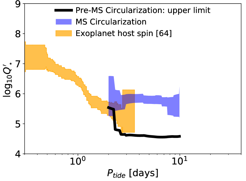
Figure 18: The constraints from this work and previous work from our group based on tidal spin-up of hot Jupiter host stars.

Two additional extensive studies of tidal dissipation in exoplanet systems are Hansen (2010) and Bonomo et al. (2017).

At first glance, the Hansen (2010) results seems inconsistent with the results presented here and by some of the other studies mentioned above. In fact, the authors themselves point that out. However, the (Hansen, 2010) dissipation estimates include systems with hosts stars that lack significant surface convective zones. In fact, one of the key systems which sets the stellar dissipation in their analysis is HAT-P-2, whose host star has a surface temperature of 6300K, slightly above the boundary where the surface convective zone becomes negligible. Furthermore, Hansen (2010) parametrize tides with a single parameter that is not uniquely related to $Q_{\star}^{\prime}$ and do not allow for the possibility that their tidal parameter is different for different systems or changes as systems evolve. This makes it impossible to isolate the dissipation their analysis would require for stars with structure similar to the ones we analyze here.

Bonomo et al. (2017) calibrate planetary and stellar tidal dissipation in HJ systems based on a similar basic idea to this study. For stellar dissipation in particular, they require that the circularization timescale for eccentric systems must be larger than the system age, and apply that limit one system at a time. They find lower limits on $Q_{\star}^{\prime}$ varying from $10^{9}$ to under $10^{5}$, correlated with the semimajor axis. The correlation with star-planet separation simply reflects the degeneracy between $Q_{\star}^{\prime}$ and semi-major axis when predicting how effective tides are at changing the orbit. These authors also make no effort to distinguish between stars with or without significant surface convection. However, since the authors treated each system separately we are able to check for that. Of the 8 shortest period systems found by Bonomo et al. (2017) to require $Q_{\star}^{\prime}>10^{6}$, half are hot (negligible surface convection): WASP-18, WASP-14, XO-3, and HAT-P-14; and the other half are cool (significant surface convection): HAT-P-16, HAT-P-20, WASP-10, and WASP-89. Furthermore, except for WASP-89, these systems have small eccentricities, meaning that the dominant tidal wave will have a period equal to half the period with which the planet goes around the star in a reference frame rotating with the star. Since these are not fast rotating stars, these periods are several days, placing the 4 cool systems in direct conflict with the results here and of some of the other studies mentioned above. One tempting explanation is that this difference is real, perhaps due to the hugely different amplitudes of the tidal waves a companion star would raise compared to a companion planet. To really compare the two results, however, one would need to properly model the entire evolution of these star-planet systems, perhaps following a similar approach to what we did here.

At first glance, our results appear to be inconsistent with Collier Cameron & Jardine (2018), who found that significantly less dissipation than we find is required to explain the observed upper boundary of the HJ population in the mass ratio — orbital separation diagram. In particular, they find that for systems expected to experience enhanced dissipation due to inertial waves (all our systems are in this regime) $\log_{10}Q_{\star}^{\prime}=7.3\pm 0.4$ is required for tidal inspiral to produce the observed edge in the distribution. However, as is evident from their Fig. 3, signatures of tidal inspiral are only detectable for orbital semimajor axes less than 3 times the Roche limit. For a Jupiter mass planet around a solar mass star this corresponds to orbital periods less than 2.5 days or tidal periods less than $\sim 2$ days, even allowing for a correction due to the stellar spin: $P_{tide}=0.5\left(P_{orb}^{-1}-P_{\star}^{-1}\right)^{-1}$ ($P_{\star}$ is the spin period of the star). Since the majority of the signal in the Collier Cameron & Jardine (2018) study comes at even shorter periods, their constraints are sensitive to the tidal dissipation below the frequnecy range probed here. These would be more appropriately compared to the Penev et al. (2018) results. Since the authors did not test for, or allow for frequnecy dependent dissipation, it is entirely possible that the two constraints are consistent. A reliable test would require repeating the Collier Cameron & Jardine (2018) analysis with a more flexible prescription for $Q_{\star}^{\prime}$.

5 Conclusions

We used available measurements of the orbital eccentricities of 38 single lined spectroscopic binaries from 3 different open clusters to infer the tidal dissipation required to simultaneously explain the observed period-eccentricity envelope in those clusters, while at the same time allowing at least the measured present day eccentricity of each system to be reproduced for reasonable choices of initial conditions.

Our analysis allowed for, but did not find evidence for powerlaw frequency dependence of the tidal dissipation; in fact, for any tidal period between 2 and 10 days, the required tidal quality factor for main-sequence stars was found to satisfy $5.5<\log_{10}Q_{\star}^{\prime}<6$, with the majority of the range constrained significantly tighter than that. However, we find significantly higher, by more than an order of magnitude, dissipation for binaries in the cluster for which tidal circularization predominantly happens during the pre-main-sequence, compared to the two clusters dominated by main-sequence circularization.

We used Bayesian analysis to properly account for observational uncertainties, and a flexible tidal model to allow for frequency dependent tidal dissipation. Our orbital evolution simulations accounted for evolving stellar structure, loss of angular momentum to stellar winds, and the internal redistribution of angular momentum between the surface and the interior of stars. Furthermore, we properly simulated tides for stars in eccentric orbits, by splitting the tidal potential into its Fourier components, and allowing for separate dissipation for each tidal wave under a common frequency dependent prescription. The only studies that account for all of these complexities (e.g. Bolmont & Mathis, 2016; Benbakoura et al., 2019) assume a particular theoretical model for the dissipation and only treat circular orbits with no spin-orbit misalignment, making them incapable of tackling the analysis presented here and preventing comparison with other tidal dissipation models than the ones assumed. The improved modeling used here resolves the internal inconsistencies of previous constraints based on these same binaries (Meibom & Mathieu, 2005; Milliman et al., 2014). For example, the circularization period Milliman et al. (2014) found for NGC 6819 was well below the claimed evolution of circularization with age, below that of even younger clusters. In the Meibom & Mathieu (2005) interpretation that would suggest this cluster has undergone less circularization than the others, hence requiring larger $Q_{\star}^{\prime}$. This should have been particularly pronounced when comparing to NGC 188, since that is the cluster with largest leverage in defining the trend of increasing circularization period on the MS. As we show here, once the particular characteristics of the individual binaries are properly accounted for, the same tidal dissipation is able to explain both NGC 188 and NGC 6819 circularization.

Data Availability

All tables of input parameters presented in this article are derivative of published tables already available in machine readable form through the VizieR online service. They are reproducible by applying simple filtering to those tables, and thus do now warrant creating and publishing independent copies.

We have created a zenodo archive (Penev & Schussler, 2022) to accompany this article, which provides machine readable tables of the following:

• The generated MCMC samples for each binary in the original HDF5 format produced by the emcee package (Foreman-Mackey et al., 2013) (see https://emcee.readthedocs.io/en/stable/user/backends/).

• The 2.3%, 15.9%, 84.1%, and 97.7% quantiles of $\log_{10}Q_{\star}^{\prime}$ for the given binary as a function of tidal period for each binary. (i.e. the coordinates defining the quantile curves in Fig. 5 — 7).

• The burn-in period for each quantile vs tidal period (i.e. the coordinates defining the burn-in curves in Fig. 8 — 10)

• The estimated standard deviation of the fraction of samples below each of the 4 target quantiles for each binary (i.e. the coordinates defining the curves in Fig. 11 — 13)

• The 84.1%, and 97.7% quantiles of the combined $\log_{10}Q_{\star}^{\prime}$ constraint from all M 35 binaries vs tidal period. Note that the lower quantiles are not constrained by the data but rather come from the assumed priors for the $log_{10}Q_{\star}^{\prime}$ model parameters.

• The 2.3%, 15.9%, 84.1%, and 97.7% quantiles of the combined $\log_{10}Q_{\star}^{\prime}$ constraint from all NGC 6819 and NGC 188 binaries vs tidal period, excluding NGC 188 binary PKM 4904 (i.e. the coordinates of the quantile curves in the bottom panel of Fig. 15).

The version of POET used for calculating the orbital evolution is available through zenodo archive Penev et al. (2022).

Appendix A Tidal Locking

Numerical expediency forces us to introduce one more wrinkle to the tidal dissipation model described in Section 2.2. In particular, POET is designed to efficiently handle discontinuities in the frequency dependence of $\Delta_{m,m^{\prime}}$ (or $Q^{\prime}_{m,m^{\prime}}$) when $\Omega_{m,m^{\prime}}=0$. This occurs if $\Delta_{m,m^{\prime}}$ does not approach zero as $\Omega_{m,m^{\prime}}\rightarrow 0$. In such cases, when a particular tidal term reaches zero frequency during the orbital evolution, it may happen that the tidal evolution equations, assuming $\Omega_{m,m^{\prime}}$ approaches zero from above and below, predict that the time derivative $\dot{\Omega}_{m,m^{\prime}}$ is negative and positive respectively. In that case, at least for some time, the spin of the zone will be locked in some integer ratio with the orbital frequency. If that situation is detected, POET eliminates the spin of the zone as an independently evolved variable. This allows the subsequent evolution to continue taking large time steps without losing accuracy or precision, but with a check of whether the lock is maintained at each subsequent step.

In the case of $\alpha<0$ in Eq. 12, such locking behavior is frequent, and the described scheme dramatically speeds up the calculations. When $\alpha>0$, exact spin-orbit locks don’t occur. However, it still frequently happens that during the evolution stable equilibrium points are encountered when some tidal term ends up with very small frequency ($\Omega_{m,m^{\prime}}=m\Omega_{\star}-m^{\prime}\Omega_{orb}\ll\Omega_{orb}$). Because the equilibrium tidal frequency evolves as the orbit evolves, it is not possible to handle these cases by eliminating one of the variables. If nothing is done in those cases however, maintaining the desired precision in calculating the evolution results in impractically small time steps. In order to avoid such extremely time consuming calculations, we tweak the tidal prescription slightly to ensure $\Delta_{m,m^{\prime}}$ remains non-zero (though small) as $\Omega_{m,m^{\prime}}\rightarrow 0$ no matter the value of $\alpha$. To be precise, when $\alpha<0$ we use Eq. 12, however when $\alpha>0$ we instead use:

$$Q^{\prime}_{m,m^{\prime}}=Q_{0}\begin{cases}\left(\frac{P_{max}}{P_{0}}\right)^{\alpha}&\text{if }P_{m,m^{\prime}}>P_{max}\\ \left(\frac{P_{m,m^{\prime}}}{P_{0}}\right)^{\alpha}&\text{if }P_{max}>P_{m,m^{\prime}}>P_{0}\\ 1&\text{if }P_{m,m^{\prime}}<P_{0}\end{cases}$$ (19)

The value of $P_{max}$ ($P_{max}=50$ days) was chosen to ensure that the calculated eccentricity and semimajor axis evolution are indistinguishable from those produced under Eq. 12, except that in some cases calculations are between 3 and 4 orders of magnitude faster using the prescription above. The effect of this tweak is shown in Fig. 19, where we compare the evolution of a fiducial binary calculated assuming exactly Eq. 12 and the modified prescription of Eq. 19. As the inset in the figure shows, the only effect is to add brief periods of spin-orbit locks each time the system evolves through one of these co-rotation resonances.

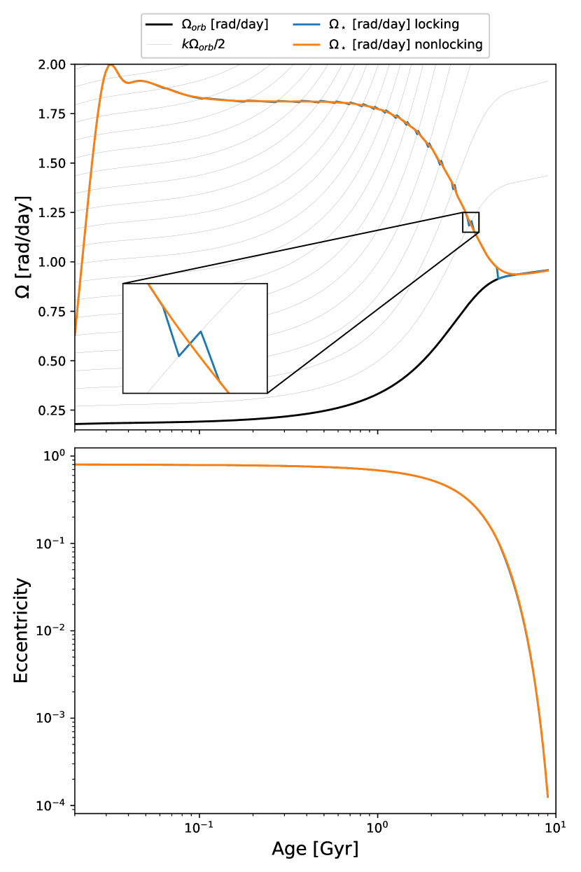
Figure 19: Top: Comparison of the orbital and stellar convective zone spin frequency evolutions calculated using Eq. 12 (non-locking) and Eq. 19 (locking) for a binary of $1\,M_{\odot}$ + $0.7\,M_{\odot}$ stars, assuming $Q_{0}=10^{6}$, $P_{0}=5$ days, and $\alpha=1$. The thin grey lines indicate possible spin-orbit locks (i.e. $2\Omega_{\star}=k\Omega_{orb}$ for some integer $k$. The inset zooms in near one such lock to show the effect of Eq. 19. Bottom: The associated eccentricity evolution. Evolution with both assumptions of tidal dissipation prescription are plotted but are indistinguishable in the plot.

Appendix B Convergence Diagnostics/Burn-in

We wish to determine how many MCMC steps must be taken in order to reliably estimate a given quantity. This question will have a different answer depending on the exact quantity being estimated. In this case, we wish to know the 2.3%, 15.9%, 84.1%, 97.7% percentiles of the distribution. We must determine how many steps are required for the starting positions to be forgotten, and how many further steps are required to get precise estimates of these quantiles.

We begin by selecting a set of 30 diagnostic tidal periods ($P_{p}$), distributed uniformly in log-space between 1 and 50 days, and quantiles levels ($q_{q}\in\{2.3\%,15.9\%,84.1\%,97.7\%\}$), matching 1- and 2-$\sigma$ quantiles of the normal distribution. Then for each sample in the MCMC chain for a particular binary system, we evaluate the tidal model (Eq. 12) at each of those periods, getting a tidal period specific chain of $\log_{10}Q_{\star}^{\prime}$ values. Let $x_{p,w,t}$ ($t\in\left\{1\ldots T\right\}$, $w\in\left\{1\ldots W\right\}$) be the value of $\log_{10}Q_{\star}^{\prime}(P_{p})$ for the $t$-th steps of the $w$-th walker.

Using kernel density estimation (with Epanechnikov kernel) we estimate the quantile $u_{p,q}$ of $\log_{10}Q_{\star}^{\prime}$ at each of the $q_{q}$ levels for each of the $P_{p}$ tidal periods. Our goal is to find a burn-in period for $u_{p,q}$, as well as an estimate of the variance of the estimated cumulative distribution of $\log_{10}Q_{\star}^{\prime}$ evaluated at $u_{p,q}$.

For each diagnostic tidal period and quantile, we begin by constructing a discrete sequence of the number of walkers at each step below a given quantile:

$$z_{p,q,t}=\sum_{w}\begin{cases}1&\mathrm{if}\ x_{p,w,t}<u_{p,q}\\ 0&\mathrm{otherwise}\end{cases}$$ (20)

As Raftery & Lewis (1991) point out, while $z_{p,q,t}$ is not necessarily a Markov process, the sufficiently thinned chain $\{z_{p,q,1+k(t-1)}\}$ will be well approximated by one if $k$ is large enough. To find $k$ Raftery & Lewis (1991) suggest using a Bayesian information criterion to determine the smallest value of $k$ at which a first order Markov process is preferred over a second order one, i.e. the first $k$ for which:

$$\log\frac{ML_{2}(\{z_{p,q,1+k(t-1)}\})}{ML_{1}(\{z_{p,q,1+k(t-1)}\})}-s(s-1)^{2}\log\lfloor\frac{T}{k}\rfloor<0$$ (21)

where $ML_{1}$ and $ML_{2}$ are the maximum likelihoods fitting $\{z_{p,q,1+k(t-1)}\}$ with a first and second order Markov processes respectively, $s$ is the number of distinct values present in $\{z_{p,q,t}\}$ (i.e. number of states the approximate Markov process samples over), and $T$ is the number of steps in the original emcee chain.

Given the matrix of maximum likelihood estimates ($P_{i,j}$) of the transition probabilities from state $i$ to state $j$ of the first order Markov process over the thinned chain, we then find the equilibrium distribution $\pi_{i}$ by solving $P\pi=\pi$. The burn-in period is then $Mk$, where $M$ is the smallest number such that the probability of being in each of the $s$ accessible states after $M$ Markov steps is within some tolerance ($\varepsilon$) of the equilibrium distribution, for all initial states:

$$(P^{M})_{i,j}-\pi_{j}\leq\varepsilon$$ (22)

We choose $\varepsilon=10^{-3}$ for this study.

Finally, in order to estimate the variance in the value of the cumulative distribution at $u_{p,q}$, we discard the burn-in samples found above and generate $10^{5}$ independent realizations of the best-fit Markov process on $\{z_{p,q,1+k(M+t-1)}\}$, and calculate their sample variance.

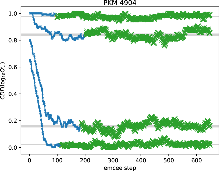
Figure 20: Demonstration of the convergence estimation algorithm. The sequence of “x” symbols shows the fraction of samples below the estimated value of each of our target quantiles vs the emcee step number. The smaller blue samples are from the estimated burn-in period and the larger green crosses are the samples we use in determining the constraints. The grey areas show the estimated standard deviation of the CDF around the target value (2.3%, 15.9%, 84.1%, 97.7% respectively) computed from the post burn-in samples.

Fig. 20 shows this algorithm applied to the binary that showed the largest drift of the estimated quantiles: NGC 188 binary PKM 4904. We see the distribution narrowing dramatically for the first 100 or so samples (the fraction of the distribution between the upper and lower boundary becomes much larger). The 15.9% percentile exhibits the largest auto-correlation and as a result the estimated burn-in period is the longest. The grey areas also show the estimated uncertainties in the values of the cumulative distribution function (the middles of these areas are the targeted quantiles) based on the post-burn-in samples.

Appendix C Effect of Binary Evolution Starting Age

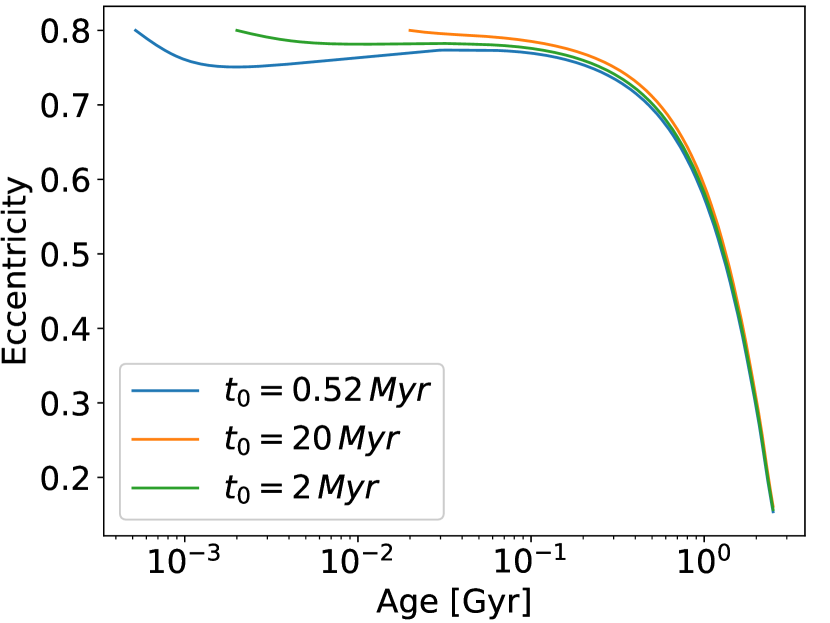
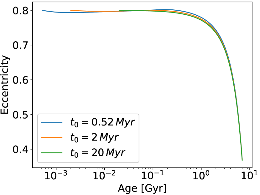
Figure 21: The negligible effect of the age at which binary evolution starts for a binary with two $1\,M_{\odot}$ stars with parameters suitable for NGC 6819 (left) and NGC 188 (right).

In Sec. 2.1 we outlined that we start calculating tidal evolution from an age of $t_{0}=20\,Myr$ for NGC 6819 and NGC 188 and $t_{0}=2\,Myr$ for M 35. The choice of starting age would justifiably raise concerns with expert readers who are familiar with findings in the literature that pre-MS evolution appears to dominate tidal circularization for the first few hundred Myrs (c.f. Meibom & Mathieu, 2005). In this appendix we demonstrate that this choice did not significantly alter the final results.

For the older clusters, Meibom & Mathieu (2005); Milliman et al. (2014) show that the tidal evolution is dominated by the main sequence. As a result, the exact details of what happens during the first few tens of Myrs are largely irrelevant for establishing the eccentricity envelope at Gyr ages. More precisely, for systems with long present day orbital period, tides hardly affect the orbit both on the MS and during PMS. At short orbital periods tides would have circularized the system by our starting age of 20 Myrs, but since MS circularization is even more important for theses systems, even omitting that initial phase, the orbit is circularized by the time we reach the age of NGC 6819 and NGC 188. The only possible concern then is with systems that are significantly, but not fully, circularized by the corresponding age of the cluster being analyzed.

Fig. 21 compares the eccentricity evolutions of a fiducial system consisting of two identical solar mass stars, assuming a constant tidal quality factor ($\log_{10}Q_{\star}^{\prime}=5.8$), starting at ages of $0.5\,Myr$, $2\,Myrs$, and $20\,Myrs$ respectively with an initial eccentricity of 0.8 and final age and orbital period corresponding to the age and tidal circularization period (per Meibom & Mathieu, 2005) of NGC 6818 (left) and NGC 188 (right). In the left panel, the system is evolved to an age of 2.5 Gyrs with a final orbital period of 8 d, and in the right panel the final age is 7 Gyrs and the final orbital period is 14.5 d. In all cases, the evolution assumed $\log_{10}Q_{\star}^{\prime}=5.8$ (the value found in this study). As can be seen, there is virtually no difference between the three assumed starting ages. This can be understood by the fact that tides do not only circularize, but also shrink the orbit over time. As a result, a system that is significantly circularized must have started with a much longer orbital period than it has today. Thus, the effect of tides accelerates over time, and must have been much smaller in the past. In other words, if MS tidal evolution dominates over the PMS, and the system is only partially circularized, it must be that initially tides were just barely effective in changing the system (approximately flat portion of the curves in Fig. 21). Note that the slight increase in eccentricity seen in the figure corresponds to the star spinning super-synchronously for a short period of time. This occurs regardless of the initial spin period chosen for the stars, since as soon as tides become important they deliver sufficient angular momentum to the stars that, as they shrinks toward the zero-age main sequence, they end up spinning faster than the orbit.

Note that if the tidal dissipation is a sufficiently strong function of age, the PMS circularization may dominate over MS circularization regardless of the binary age. In this case, the age at which tidal evolution turns on will be important. However, that contradicts the Meibom & Mathieu (2005) and Milliman et al. (2014) observation that the circularization period gradually increases over the MS. Furthermore, since our prescription for $Q_{\star}^{\prime}$ (Eq. 12) does not incorporate an explicit age dependence, repeating the analysis with a different starting age will not change our results.

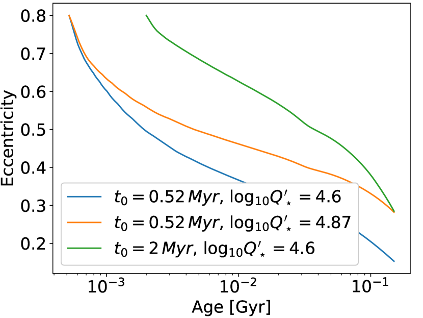
Figure 22: The effect of the age at which binary evolution starts for a binary with two $1\,M_{\odot}$ stars with parameters suitable for M 35.

The situation is a little less straightforward for M 35 than for the older clusters. The Meibom & Mathieu (2005) circularization period for this cluster is consistent with that of all younger clusters. This is usually interpreted to imply that the circularization for such young systems is dominated by the evolution at young ages when the star is large and hence subject to much stronger tides. This is why we use a much smaller starting age (2 Myrs) when constraining the dissipation in the 150 Myr old M 35. This was chosen as a compromise. At much younger ages, the rapid evolution of the radius and internal structure of Sun-like stars caused numerical instabilities in the calculated orbital evolution for some systems. At the same time, the effect on the inferred tidal dissipation of starting at 2 Myrs versus a much younger age is sufficiently small to not compromise the results. Fig. 22 compares the eccentricity evolutions of a binary consisting of two $1\,M_{\odot}$ stars started with an initial eccentricity of 0.8 and initial orbital period such that at an age of 150 Myrs the system evolves to have an orbital period of 10.2 days (the tidal circularization period Meibom & Mathieu, 2005, report for M 35). For the top and bottom curves, evolution was calculated assuming $\log_{10}Q_{\star}^{\prime}=4.6$ (the upper limit found here). Clearly, in this case, changing the starting age has a non-negligible effect on the final eccentricity. However, the effect on the inferred value of $\log_{10}Q_{\star}^{\prime}$ is quite limited. The middle curve shows the evolution calculated with the smaller starting age, but with $\log_{10}Q_{\star}^{\prime}=4.87$, which reproduces the same final eccentricity as the evolution started at $2\,Myrs$. As discussed above, choosing a system that is significantly, but not completely, circularized is the worst-case scenario for the effect of the starting age. As a result, we can conclude that pushing the starting age to $2\,Myr$ can at most change the inferred value of $\log_{10}Q_{\star}^{\prime}$ by no more than 0.3 dex.

Appendix D Effect of Initial Stellar Spin

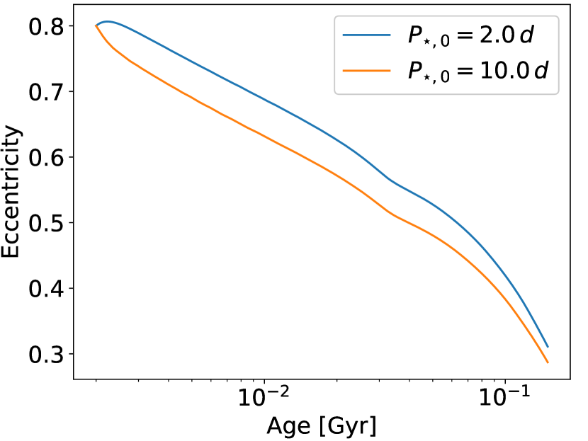
Figure 23: The effect of the initial stellar spin for the binary evolution of two $1\,M_{\odot}$ stars with parameters suitable for M 35.

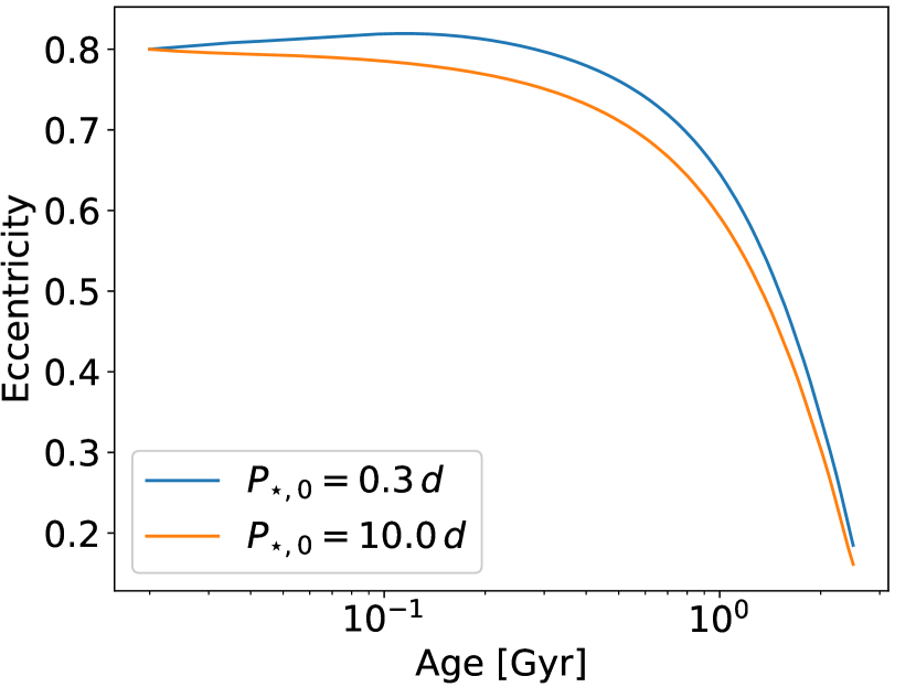
Figure 24: The effect of the initial stellar spin for the binary evolution of two $1\,M_{\odot}$ stars with parameters suitable for NGC 6819.

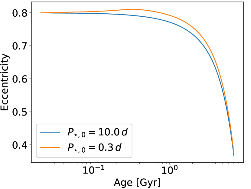
Figure 25: The effect of the initial stellar spin for the binary evolution of two $1\,M_{\odot}$ stars with parameters suitable for NGC 188.

Another reasonable concern with assumptions made in our modeling has to do with the initial spin assumed for the stars. In particular, we assume binary evolution always starts with both stars having a surface spin period of 10 d. Observations of young stars show a range of initial rotation periods. In particular, Gallet & Bouvier (2015) report spin periods ranging from about 2 d to about 8 d for single stars with ages of a few Myr (relevant for our M 35 simulations). As stars shrink toward the main sequence from these initial spins, the range shifts to 0.3 — 7 d for ages of 20 Myrs (the assumed starting age for NGC 6819 and NGC 188 in this analysis). In Fig. 23, 24, and 25 we show that the assumed initial spin has only a negligible effect on the eccentricity evolution, as long as it remains within the observed ranges. This also makes intuitive sense, because stellar spin accounts for only a very small fraction of the total angular momentum in the system, so exchanging part of that with the orbit can only have a small effect on the final eccentricity. The impact of different assumed values for the initial spin are further suppressed by the fact that faster spinning stars lose angular momentum to magnetic winds faster (Gallet & Bouvier, 2015).

The effect of the initial spin may be somewhat larger than in Fig. 23, 24, and 25 if the tidal dissipation were to increase sufficiently quickly with increasing stellar spin. However, even in that case, the effect will be limited as the orbital angular momentum far exceeds the spin angular momentum of the individual stars even for the fastest observed initial spins. Since the parametrization used in this analysis (Eq. 12) does not include explicit spin dependence, our results would not significantly change if we were to allow the initial spin to vary.

References

- Abdelaziz et al. (2022) Abdelaziz A., Saad S., Hendy Y., Shokry A., Kamal F., 2022, New Astronomy, 92, 101727
- Alexander (1973) Alexander M. E., 1973, Ap&SS, 23, 459
- Anderson et al. (2021) Anderson K. R., Winn J. N., Penev K., 2021, ApJ, 914, 56
- Barker (2020) Barker A. J., 2020, MNRAS, 498, 2270
- Barker (2022) Barker A. J., 2022, ApJ, 927, L36
- Barker & Ogilvie (2010) Barker A. J., Ogilvie G. I., 2010, MNRAS, 404, 1849
- Barnes & Sofia (1996) Barnes S., Sofia S., 1996, ApJ, 462, 746