Theoretical bound of the efficiency of learning

Abstract

A unified thermodynamic formalism describing the efficiency of learning is proposed. First, we derive an inequality, which is more strength than Clausius’s inequality, revealing the lower bound of the entropy-production rate of a subsystem. Second, the inequality is transformed to determine the general upper limit for the efficiency of learning. In particular, we exemplify the bound of the efficiency in nonequilibrium quantum-dot systems and networks of living cells. The framework provides a fundamental trade-off relationship between energy and information inheriting in stochastic thermodynamic processes.

Thermodynamic inequalities have laid the foundations of achieving useful limits on entropy production and energy. Tightening the bounds on these quantities will not only help us to develop a deeper understanding of thermodynamics but also provide insights into micro systems. It have been found that thermodynamic inequalities may strengthen Clausius’s inequality of the second law of thermodynamics Vu2021 ; Aurell2011 ; Vu202111 ; Tajima2021 ; Shiraishi2018 ; Funo2019 ; Barato2015 ; Pietzonka2018 ; Crooks2007 ; Salamon1983 ; Sivak2012 ; Scandi2019 ; Chen2021 .

In recent years, many studies have begun to focus on the role of information in thermodynamics. The most celebrated relationship between information and thermodynamics is Landauer’s principle Landauer1961 , which explicitly shows the amount of heat dissipation required to erase information in the slow quasistatic limit Dong2011 ; Hashimoto2022 ; Goold2015 ; Campbell2017 ; Hashimoto2020 . Experimental verifications of this principle have been conducted in classical and quantum regimes Dago2021 ; B=0000E9rut2012 . As modern computing alliances demand high-speed information processing, an important advance is to investigate the energy cost associated with the finite-time information erasure Vu2022 ; Proesmans2020 ; Zhen2021 .

Understanding the relation between Clausius’s inequality and information is critical to better drive the thermodynamic processes. The description of a system at a coarse-grained level may hold the key to determine the role of information in thermodynamics Esposito2012 . General formalisms quantifying the information-related contribution in Clausius’s inequality have been established for systems undergoing classical and quantum dynamics Ptaszy=000144ski2019 ; Horowitz2014 ; Strasberg2017 . For the bipartite system, the entropy production of a subsystem involves the transfer of information entropy due to its coupling with the other subsystem Hartich2014 . Based on the perspective of stochastic thermodynamics, the conditions for the optimal learning for a neuron described by a single-layer perceptron have been analyzed Goldt2017 . The rate of information exchange was regarded as the learning rate, which determines the informational efficiencies of three different models of cellular information processing Barato2014 . In linear irreversible thermodynamics, the Onsager reciprocity holds true for coefficients associated with the thermodynamic and informational affinities Yamamoto20161 .

However, it is unclear whether a tight bound on the irreversible entropy production in connection with information exists. Although the Clausius inequality may characterize the thermodynamic cost for an informational learning process, there is still no unified view on the fundamental upper bound on the efficiency of information learned. The investigation into this aspect may lead to the essential relationship between energy and information.

In this Letter, we tackle this problem and reveal the universal bound for the efficiency of learning in stochastic thermodynamic processes described by the Markovian master equation. To achieve this goal, we start from the Shannon entropy, derive Clausius’s inequality, and clarify how information is generated. Our main result shows that the entropy-production rate of a subsystem has a strict lower limit, which offers a restriction on the efficiency of learning. In particular, we show that the bound of the efficiency is applicable to every physical model, including quantum dots and living cells, as long as the principle of detailed balance is satisfied. Our framework provides a fundamental trade-off inequality by showing how to use minimum resources to achieve a desired result in the learning process.

Efficiency of learning—We follow a standard stochastic process for a bipartite system $Z$. The state of $Z$ is labeled as $z=(x,y)$, where the variables $x$ and $y$ represent the number of particles in subsystems $X$ and $Y$, respectively. The time-dependent probability $p(z)$ of state $z$ evolves according to the Markovian master equation Breuer2002 ; Kampen2007

$$\dot{p}(z)=\sum_{z^{\prime},v}J_{zz^{\prime}}^{v}.$$ (1)

Here, the current $J_{zz^{\prime}}^{v}=W_{zz^{\prime}}^{v}p(z^{\prime})-W_{z^{\prime}z}^{v}p(z)$ depends on the time-independent transition rate $W_{zz^{\prime}}^{v}$ from state $z^{\prime}$ to state $z$ induced by reservoir $v$ and the rate $W_{z^{\prime}z}^{v}$ of the reverse transition process. The transition rate matrix is non-negativity $W_{zz^{\prime}}^{v}\geq 0$ for $z\neq z^{\prime}$. The bipartite structure does not allow the two subsystems to change the states simultaneously. Thus, the form of $W_{zz^{\prime}}^{v}$ is restricted to Horowitz2014 ; Hartich2014

$$W_{zz^{\prime}}^{v}=\begin{cases}W_{xx^{\prime}\mid y}^{v},&\left(x\neq x^{\prime},y=y^{\prime}\right)\\ W_{yy^{\prime}\mid x}^{v},&\left(x=x^{\prime},y\neq y^{\prime}\right)\\ 0\text{,}&\text{ (otherwise) }\end{cases}$$ (2)

where $W_{xx^{\prime}\mid y}^{v}$ is the transition rate of subsystem $X$ from state $x^{\prime}$ to state $x$ under the condition that subsystem $Y$ is at state $y$, and similarly for $W_{yy^{\prime}\mid x}^{v}$.

The coarse-grained dynamics of subsystem $X$ is formally written as Zhen2021 ; Esposito2012

$$\dot{p}\left(x\right)=\sum_{x^{\prime},v}\left[V_{xx^{\prime}}^{v}p\left(x^{\prime}\right)-V_{x^{\prime}x}^{v}p\left(x\right)\right]=\sum_{x^{\prime},y,v}J_{xx^{\prime}\mid y}^{v},$$ (3)

where the marginal probability $p\left(x\right)$ is calculated by summing $p\left(x,y\right)$ over the variable $y$, i.e., $p\left(x\right)=\sum_{y}p\left(z\right)=\sum_{y}p\left(x,y\right)$, the transition rate $V_{xx^{\prime}}^{v}=\sum_{y}W_{xx^{\prime}\mid y}^{v}p\left(y|x^{\prime}\right)$ with $p\left(y|x^{\prime}\right)=p\left(x^{\prime},y\right)/p\left(x^{\prime}\right)$ being the conditional probability, and $J_{xx^{\prime}\mid y}^{v}=W_{xx^{\prime}\mid y}^{v}p\left(x^{\prime},y\right)-W_{x^{\prime}x\mid y}^{v}p(x,y)$ is the current from state $x^{\prime}$ to state $x$ provided that subsystem $Y$ is at state $y$.

Starting from the time derivative of Shannon’s entropy $S^{X}=-\sum_{x}p\left(x\right)\ln p\left(x\right)$ and inserting Eq. (3), one obtains the entropy-production rate $\dot{\sigma}^{X}$ of subsystem $X$ (see Supplemental Material, Sec. I and Sec. II)

$$\dot{\sigma}^{X}=\dot{S}^{X}+\dot{S_{r}}^{X}-\dot{I}^{X}\geq 0\text{,}$$ (4)

where

$$\dot{\sigma}^{X}=\frac{1}{2}\sum_{x,x^{\prime},y,v}J_{xx^{\prime}\mid y}^{v}\ln\frac{p\left(x^{\prime},y\right)W_{xx^{\prime}\mid y}^{v}}{p\left(x,y\right)W_{x^{\prime}x\mid y}^{v}}\geq 0,$$ (5)

$$\dot{S_{r}}^{X}=\frac{1}{2}\sum_{x,x^{\prime},y,v}J_{xx^{\prime}\mid y}^{v}\ln\frac{W_{xx^{\prime}\mid y}^{v}}{W_{x^{\prime}x\mid y}^{v}}\text{,}$$ (6)

$$\dot{I}^{X}=\frac{1}{2}\sum_{x,x^{\prime},y,v}J_{xx^{\prime}\mid y}^{v}\ln\frac{p\left(y|x\right)}{p\left(y|x^{\prime}\right)}.$$ (7)

Note that the overdot notation, as in $\dot{\sigma}^{X}$, $\dot{S_{r}}^{X}$, and $\dot{I}^{X},$ is used to emphasize that such quantities are rates. The rate $\dot{\sigma}^{X}$ is always positive due to the fact that $p\left(x,y\right)W_{x^{\prime}x\mid y}^{v}\geqslant 0\forall x\neq x^{\prime}$ and $J_{xx^{\prime}\mid y}^{v}\ln\frac{p\left(x^{\prime},y\right)W_{xx^{\prime}\mid y}^{v}}{p\left(x,y\right)W_{x^{\prime}x\mid y}^{v}}\geqslant 0$ Zhen2021 , satisfying the second law of thermodynamics. $\dot{S_{r}}^{X}$ is the entropy flow to the environment, which is associated with the energy flux from $X$ into the environment. $\dot{I}^{X}$ quantifies the rate of information learned. When $\dot{I}^{X}>0$, $X$ acts as a sensor, creating information by learning $Y$. On the other hand, $\dot{I}^{X}<0$ means that $Y$ is learning $X$ and the information learned is being erasured or consumed by $X$ for extracting energy or doing work Horowitz2014 . Equivalent expressions from Eq. (4) to Eq. (7) can be developed for subsystem $Y$. In Ref. Hartich2014 , Hartich interpreted $\dot{I}^{X}$ as the rate of the entropy reduction of subsystem $X$ due to its coupling with $Y$.

At the steady state, the system reaches the stationary probability distribution $\left[\dot{p}\left(x\right)=0\right]$, and thus $\dot{S}^{X}=0$. Therefore, Eq. (5) is simplified into

$$\dot{\sigma}^{X}=\dot{S_{r}}^{X}-\dot{I}^{X}\geq 0.$$ (8)

In the case of $\dot{I}^{X}>0$, Eq. (8) dictates that the rate of information learned is bounded by the entropy flow to the environment $\dot{S_{r}}^{X}$, which characterizes the dissipation necessary for $X$ learning about $Y$. Information will provide the resource for extracting energy or doing work through the feedback on $Y$. From inequality (8), the efficiency of learning is defined as

$$\eta^{X}=\frac{\dot{I}^{X}}{\dot{S_{r}}^{X}}\leq 1.$$ (9)

It determines the effectiveness of learning and has been widely adopted Goldt2017 ; Barato2014 ; Hartich2014 .

Theoretical bound of the efficiency of learning—Our aim is to evaluate the upper bound of the efficiency of learning. To this end, we first present an alternative lower limit on $\dot{\sigma}^{X}$, i.e.,

$$\sqrt{\dot{\sigma}^{X}}\geq\left|\dot{S_{r}}^{X}\right|/\sqrt{\Theta^{X}},$$ (10)

where

$$\Theta^{X}=\frac{1}{2}\sum_{x,x^{\prime},y,v}\left(\ln\frac{W_{xx^{\prime}\mid y}^{v}}{W_{x^{\prime}x\mid y}^{v}}\right)^{2}W_{xx^{\prime}\mid y}^{v}p\left(x^{\prime},y\right)\text{.}$$ (11)

The Cauchy-Schwartz inequality Shiraishi2018 ; Funo2019 and the inequality $\frac{(x-y)^{2}}{x+y}\leq\frac{x-y}{2}\log\frac{x}{y}$ for non-negative $x$ and $y$ have been applied in the proof (see Supplemental Material, Sec. III). Eq. (10) provides a restriction stronger than the value claimed by Eq. (8). By supposing that $\dot{S_{r}}^{X}\geq 0$ and $\dot{I}^{X}\geq 0$, a universal lower bound for the efficiency of learning is given by (see Supplemental Material, Sec. III)

$$\eta^{X}\leq 1-\frac{\dot{S_{r}}^{X}}{\Theta^{X}}.$$ (12)

This bound, which is the main result of this Letter, is applicable to every physical model as long as the principle of detailed balance is satisfied. The physical meaning of the inequalities (10) and (12) is obvious. If bath $v$ induces a transition from state $\left(x^{\prime},y\right)$ to state $\left(x,y\right)$, the energy absorbed by the system is simply written as $E\left(x,y\right)-E\left(x^{\prime},y\right)=-k_{B}T_{v}\ln\frac{W_{xx^{\prime}\mid y}^{v}}{W_{x^{\prime}x\mid y}^{v}}$, where $E\left(x,y\right)$ is the energy of state $\left(x,y\right)$, $k_{B}$ is the Boltzmann constant, and $T_{v}$ denotes the temperature of bath $v$. $W_{xx^{\prime}\mid y}^{v}p\left(x^{\prime},y\right)$ quantifies the frequency of the jump between given states. Therefore, the coefficient $\Theta^{X}$ can be regarded as a dynamic activity factor. On the other hand, the rate $\dot{S_{r}}^{X}$ originates from the irreversible energy loss to the environment. The inequalities (10) and (12) manifest a trade-off between the speed of the energy exchange and the dissipation.

Numerical demonstration.—In the following, a quantum system and a cellular network, where information and thermodynamics can be intuitively related via the Clausius inequality, will be used to exemplify our findings. We demonstrate that the efficiency of learning is well characterized by the inequality in (12).

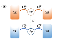
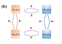
Figure 1: (a) The schematic diagram of a double-quantum-dot system. (b) The schematic representation of a cellular network.

The double-quantum-dot system.—The double-quantum-dot (DQD) system consists of two quantum dots interacting via a Coulomb repulsion $U$. The DQD [See Fig. 1(a)] is modeled by the Hamiltonian

$$H_{S}=\varepsilon_{X}d_{X}^{\dagger}d_{X}+\varepsilon_{Y}d_{Y}^{\dagger}d_{Y}+Ud_{X}^{\dagger}d_{X}d_{Y}^{\dagger}d_{Y},$$ (13)

where $d_{X}^{\dagger}$ ($d_{X}$ ) creates (annihilates) one electron on QD $X$ with energy $\varepsilon_{X}$, and $d_{Y}^{\dagger}$ ($d_{Y}$ ) creates (annihilates) one electron on QD $Y$ with energy $\varepsilon_{Y}$. QD $X\left(Y\right)$ is weakly coupled to two Fermi reservoirs $XL$ and $XR$ ($YL$ and $YR$). Thus, electrons are transported through parallel interacting channels. The Hamiltonian of the reservoirs is given by

$$H_{B}=\sum_{k}\sum_{\alpha\in\{X,Y\}}\sum_{\beta\in\{L,R\}}\varepsilon_{k\alpha\beta}c_{k\alpha\beta}^{\dagger}c_{k\alpha\beta},$$ (14)

where $c_{k\alpha\beta}^{\dagger}\left(c_{k\alpha\beta}\right)$ is the creation (annihilation) operator at energy level $\varepsilon_{k\alpha\beta}$ in bath $\alpha\beta$. The interaction between the DQD and the environment reads

$$H_{I}=\sum_{k}\sum_{\alpha\in\{X,Y\}}\sum_{\beta\in\{L,R\}}\left(t_{k\alpha\beta}d_{\alpha}c_{k\alpha\beta}^{\dagger}+t_{k\alpha\beta}^{\text{\textasteriskcentered}}c_{k\alpha\beta}d_{\alpha}^{\text{\textdagger}}\right),$$ (15)

where $t_{k\alpha\beta}$ denotes the coupling strength of the transition between QD $\alpha$ and reservoir $\alpha\beta$ at energy level $\varepsilon_{k\alpha\beta}$. We use $x_{0}$ and $y_{0}$ ($x_{1}$ and $y_{1}$) to denote that $X$ and $Y$ are in empty (filled) states, respectively. The energy eigenstates of the DQD coincide with the localized Fock states $\left|\left(x_{0},y_{0}\right)\right\rangle,\left|\left(x_{1},y_{0}\right)\right\rangle,\left|\left(x_{0},y_{1}\right)\right\rangle$, and $\left|\left(x_{1},y_{1}\right)\right\rangle$, where their respective eigenvalues are $0$, $\varepsilon_{X}$, $\varepsilon_{Y}$, and $\varepsilon_{X}+\varepsilon_{Y}+U$.

For a non-degenerate system weakly coupled to different environmental modes, the dynamics of the populations satisfies Eq. (1) Strasberg2013 ; Schaller2014 . The transition rates follow from Fermi’s golden rule and are given by

$$W_{x_{1}x_{0}\mid y_{i}}^{v}=\Gamma_{y_{i}}^{v}f_{y_{i}}^{v},$$

$$W_{x_{0}x_{1}\mid y_{i}}^{v}=\Gamma_{y_{i}}^{v}\left(1-f_{y_{i}}^{v}\right),$$

$$W_{y_{1}y_{0}\mid x_{i}}^{v}=\Gamma_{x_{i}}^{v}f_{x_{i}}^{v},$$

$$W_{y_{0}y_{1}\mid x_{i}}^{v}=\Gamma_{x_{i}}^{v}\left(1-f_{x_{i}}^{v}\right),$$

where $f_{x_{i}}^{v}=\left\{1+\exp\left[\beta_{v}\left(\varepsilon_{Y}+\mathrm{\mathit{i}}U-\mu_{v}\right)\right]\right\}^{-1}$ and $f_{y_{i}}^{v}=\left\{1+\exp\left[\beta_{v}\left(\varepsilon_{X}+\mathrm{\mathit{i}}U-\mu_{v}\right)\right]\right\}^{-1}$ $(i=0,1)$ are the Fermi distribution functions, $\beta_{v}=1/\left(k_{\mathrm{B}}T_{v}\right)$, and $\Gamma_{y_{i}}^{v}\left(\Gamma_{x_{i}}^{v}\right)$ is a positive constant that characterizes the height of the potential barrier between $X$ ($Y$) and reservoir $v$. The potential barrier of $Y$, characterized by $\Gamma_{x_{i}}^{v}$, depends on the state of $X$, and vice versa.

For the purpose of reducing the number of parameters, the energy dependences of the tunneling rates are parametrized by dimensionless parameters $\delta$ and $\Delta$, i.e.,

$$\Gamma_{x_{0}}^{YL} =\Gamma\frac{e^{\Delta}}{\cosh(\Delta)}, \Gamma_{x_{1}}^{YL}=\Gamma\frac{e^{-\Delta}}{\cosh(\Delta)},$$ (16)

$$\Gamma_{x_{0}}^{YR} =\Gamma\frac{e^{-\Delta}}{\cosh(\Delta)}, \Gamma_{x_{1}}^{YR}=\Gamma\frac{e^{\Delta}}{\cosh(\Delta)},$$

$$\Gamma_{y_{0}}^{XL} =\Gamma\frac{e^{\delta}}{\cosh(\delta)}, \Gamma_{y_{1}}^{XL}=\Gamma\frac{e^{-\delta}}{\cosh(\delta)},$$

$$\Gamma_{y_{0}}^{XR} =\Gamma\frac{e^{-\delta}}{\cosh(\delta)}, \Gamma_{y_{1}}^{XR}=\Gamma\frac{e^{\delta}}{\cosh(\delta)}.$$

According to Eqs. (6), (7), and (11), the entropy flow associated with subsystem $X$

$$\dot{S_{r}}^{X}=-\beta\Delta\mu_{X}\left(J_{x_{0}x_{1}\mid y_{0}}^{XR}+J_{x_{0}x_{1}\mid y_{1}}^{XR}\right)-\beta U\left(J_{y_{1}y_{0}\mid x_{0}}^{YL}+J_{y_{1}y_{0}\mid x_{0}}^{YR}\right),$$ (17)

the rate of information learned

$$\dot{I}^{X}=\left(J_{y_{1}y_{0}\mid x_{0}}^{YL}+J_{y_{1}y_{0}\mid x_{0}}^{YR}\right)\ln\frac{p\left(x_{0},y_{1}\right)p\left(x_{1},y_{0}\right)}{p\left(x_{0},y_{0}\right)p\left(x_{1},y_{1}\right)},$$ (18)

and the coefficient

$$\Theta^{X} =\frac{1}{2}\left(\varepsilon_{X}-\mu_{XL}\right)^{2}\left[W_{10\mid 0}^{XL}p\left(0,0\right)+W_{01\mid 0}^{XL}p\left(1,0\right)\right]$$

$$+\frac{1}{2}\left(\varepsilon_{X}-\mu_{XR}\right)^{2}\left[W_{10\mid 0}^{XR}p\left(0,0\right)+W_{01\mid 0}^{XR}p\left(1,0\right)\right]$$

$$+\frac{1}{2}\left(\varepsilon_{X}+U-\mu_{XL}\right)^{2}\left[W_{10\mid 1}^{XL}p\left(0,1\right)+W_{01\mid 1}^{XL}p\left(1,1\right)\right]$$

$$+\frac{1}{2}\left(\varepsilon_{X}+U-\mu_{XR}\right)^{2}\left[W_{10\mid 1}^{XR}p\left(0,1\right)+W_{01\mid 1}^{XR}p\left(1,1\right)\right].$$ (19)

The cellular network.—In a living cell, a protein inside the cell may be phosphorylation and dephosphorylation through the consumption of energy provided by adenosine triphosphate (ATP). The receptors on the surface of the cell are either bound by ligands or empty. It is assumed that the receptors are occupied by ligands and immediately change into the inactive state $y_{0}$ when the concentration of the ligand is high. On the other hand, if the concentration is low, the receptors are unbound and become active represented by state $y_{1}$. The transitions between state $y_{0}$ and $y_{1}$ happen at the rate $\gamma$, because the concentration of the ligand in the environment jumps between low and high values. The rates of the reactions of the protein depend on the concentration of the ligand. For simplicity, we consider the following reaction equation Barato2014 ; Barato2013 ; Mehta2012

$$x_{0}+ATP\stackrel{{\scriptstyle[}}{{\kappa}}_{-}]{\kappa_{+}}{\rightleftharpoons}x_{1}+ADP\stackrel{{\scriptstyle[}}{{\omega}}_{-}]{\omega_{+}}{\rightleftharpoons}x_{0}+ADP+P_{i},$$ (20)

where $\kappa_{+}$ and $\omega_{+}$ are, respectively, the rates of phosphorylation and dephosphorylation, and $\kappa_{-}$ and $\omega_{-}$ represent the rates of the corresponding reversed processes. The phosphorylation allows the protein to change from the inactive state $x_{0}$ to the active state $x_{1}$ by the attachment of a phosphate $P_{i}$, while ATP is simultaneously converted to adenosine diphosphate (ADP). The dephosphorylation occurs when the protein gives a phosphate $P_{i}$ to ADP and turns from the active state $x_{1}$ back to the inactive state $x_{0}$. The reactions are driven by the chemical potential difference $\Delta\mu\equiv\mu_{{\rm ATP}}-\mu_{{\rm ADP}}-\mu_{{\rm P}}$, which is related to the rates in the reactions through $\Delta\mu=k_{B}T{\rm ln}[\kappa_{+}\omega_{+}/(\kappa_{-}\omega_{-})]$ with $T$ being the temperature of the cell. The active receptors arouse the process of phosphorylation in the cell. If the concentration is high, only dephosphorylation occurs due to the inactive receptors. As a summary, the low concentration implies that the receptors become active and only phosphorylation takes place. The full network of the four-state model is shown in Fig. 1 (b). The transition rates are represented by

$$W_{x_{1}x_{0}\mid y_{0}} =\omega_{-},$$

$$W_{x_{0}x_{1}\mid y_{0}} =\omega_{+},$$

$$W_{x_{1}x_{0}\mid y_{1}} =\kappa_{+},$$

$$W_{x_{0}x_{1}\mid y_{1}} =\kappa_{-},$$

$$W_{y_{1}y_{0}\mid x_{0}} =W_{y_{0}y_{1}\mid x_{0}}=W_{y_{1}y_{0}\mid x_{1}}=W_{y_{0}y_{1}\mid x_{1}}=\gamma.$$

In the stationary state, the probability current $J$ is given by

$$J =\gamma\left[p\left(x_{1},y_{1}\right)-p\left(x_{1},y_{0}\right)\right]$$

$$=\frac{\gamma}{2}\frac{\kappa_{+}\omega_{+}-\kappa_{-}\omega_{-}}{\gamma\left[\kappa_{+}+\kappa_{-}+\omega_{+}+\omega_{-}\right]+\left(\kappa_{+}+\kappa_{-}\right)\left(\omega_{+}+\omega_{-}\right)}.$$ (21)

According to Eqs. (6), (7), and (11), the entropy flow to the reservoir associated with the protein (subsystem $X$)

$$\dot{S_{r}}^{X}=J\Delta\mu,$$ (22)

the rate of information learned

$$\dot{I}^{X}=J\ln\frac{p\left(x_{1},y_{1}\right)p\left(x_{0},y_{0}\right)}{p\left(x_{0},y_{1}\right)p\left(x_{1},y_{0}\right)},$$ (23)

and the coefficient

$$\Theta^{X} =\frac{1}{2}\left(\ln\frac{\kappa_{+}}{\kappa_{-}}\right)^{2}\left[\kappa_{-}p\left(x_{1},y_{1}\right)+\kappa_{+}p\left(x_{0},y_{1}\right)\right]$$

$$+\frac{1}{2}\left(\ln\frac{\omega_{+}}{\omega_{-}}\right)^{2}\left[\omega_{+}p\left(x_{1},y_{0}\right)+\omega_{-}p\left(x_{0},y_{0}\right)\right].$$ (24)

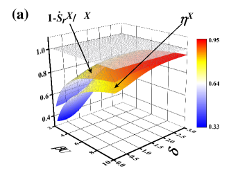
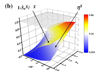
Figure 2: (a) The efficiency $\eta^{X}$ and the upper limit $1-\frac{\dot{S_{r}}^{X}}{\Theta^{X}}$ for the double-quantum-dot system varying with the dimensionless Coulomb interaction strength $\beta U$ and the parameter $\delta$ associated with the tunneling rate, where $\beta\left(\mu_{XR}-\mu_{XL}\right)=1$, $\beta\left(\mu_{YR}-\mu_{YL}\right)=2$, $\Delta=1$, $\Gamma=1$ $\varepsilon_{X}=\frac{\left(\mu_{XR}+\mu_{XL}\right)}{2}-\frac{U}{2}$, and $\varepsilon_{Y}=\frac{\left(\mu_{YR}+\mu_{YL}\right)}{2}-\frac{U}{2}$. (b) The efficiency $\eta^{X}$ and the upper limit $1-\frac{\dot{S_{r}}^{X}}{\Theta^{X}}$ for the cellular network varying with the transition rate $\gamma$ and the chemical potential difference $\Delta\mu$, where $\omega_{+}=\kappa_{+}=\exp(\Delta\mu/2)$ and $\omega_{-}=\kappa_{-}=1$.

Discussion.—For the DQD system, the efficiency $\eta^{X}$ of learning is always a monotonically increasing of $\delta$ for fixed $\beta U$ [Fig. 2 (a)]. The transition rates $\Gamma_{y_{0}}^{XL}\rightarrow 1$, $\Gamma_{y_{0}}^{XR}\rightarrow 0$, $\Gamma_{y_{1}}^{XL}\rightarrow 0$, and $\Gamma_{y_{1}}^{XR}\rightarrow 1$ with a large value of $\delta$. It parametrizes the case where an electron can only enter and exit subsystem $X$ from reservoir $XL$ at energy $\varepsilon_{X}$, whereas the tunneling process to reservoir $XR$ is allowed at energy $\varepsilon_{X}+U$. Thus, electron transport is only permitted by exchanging energy with subsystem $Y$. As a result, the two QDs become highly correlated, since subsystem $X$ is capable of rapidly adapting to the variation of the state in subsystem $Y$ by tracking and giving feedback on $Y$. When $\delta$ and $\beta U$ are both small, $\eta^{X}$ is quite small, meaning that the energy provided by reservoirs cannot effectively support the learning process. Fig. 2 (a) also displays that the relation $\eta^{X}\leq 1-\dot{S_{r}}^{X}/\Theta^{X}\leq 1$ always holds, which clearly shows the tightness of the bound in Eq. (12). In the region where $\delta$ and $\beta U$ become relatively large, $\eta^{X}$ gets closer to 1 and simultaneously the upper limit $1-\dot{S_{r}}^{X}/\Theta^{X}$ may be saturated. The upper bound indeed characterizes the cost necessary for $X$ learning about $Y$.

For the cellular network, the reaction rates of phosphorylation and dephosphorylation depend on the concentration of the ligand in the environment. Eqs. (22) and (23) demonstrate the tight coupling between $\dot{S_{r}}^{X}$ and $\dot{I}^{X}$, since they are both proportional to the probability current $J$. Therefore, $\dot{I}^{X}$ is bounded by the rate of ATP consumption, leading to the efficiency $\eta^{X}<1$ [Fig. 2(b)] and $f=\ln\frac{p\left(x_{1},y_{1}\right)p\left(x_{0},y_{0}\right)}{p\left(x_{0},y_{1}\right)p\left(x_{1},y_{0}\right)}\text{<}\Delta\mu$. For $\gamma\rightarrow 0$, Eq. (21) indicates that $J$ goes to zero. However, the maximal efficiency $\eta^{X}$is reached [Fig. 2(b)] because of $f\rightarrow\Delta\mu$. As $\gamma$ increases, the network beomes inefficient with the rate of information learned $\dot{I}^{X}$ approaching zero and a maximal ATP consumption for a given $\Delta\mu$. No matter how the transition rate $\gamma$ and the chemical potential difference $\Delta\mu$ change, the conclusion $\eta^{X}\leq 1-\dot{S_{r}}^{X}/\Theta^{X}\leq 1$ is always true as well [Fig. 2(b)]. Thus, the cellular network confirms the tightness of the bound in Eq. (12) as well.

The fundamental trade-off inequalities (10) and (12) have been proven to be effective in general Markovian stochastic processes. It is worth investigating the extension of the results to the systems with quantum effects. For example, one could exploit quantum coherence for increasing the efficiency of learning. In addition, by modelling a system as a complex network, a topological analysis could be performed to identify which type of thermodynamic flux and affinity is fundamental to the enhancement of the performance of a informational learning process.

Conclusions.—The fundamental trade-off inequalities (10) and (12) in general Markovian stochastic processes have been established. It is claimed that the entropy-production rate of a subsystem closely depends on the rate of information learned, and has a lower limit associated with the irreversible energy loss and the entropy flow to the environment. The limit imposes a constraint stronger than the conventional second law, which plays a vital role in determining the universal upper bound for the efficiency of learning. A quantum system and a cellular network that both satisfy the stochastic detailed balance condition have been used to exemplify the inequalities. The results reveal a hidden universal law inheriting in general informational learning processes.

Acknowledgments.—This work has been supported by the National Natural Science Foundation (Grants No. 12075197) and the Fundamental Research Fund for the Central Universities (No. 20720210024) of China.

References

- (1) T. V. Vu and Y. Hasegawa, Geometrical Bounds of the Irreversibility in Markovian Systems, Phys. Rev. Lett. 126, 010601 (2021).
- (2) E. Aurell, C. Mejía-Monasterio, and P. Muratore-Ginanneschi, Optimal Protocols and Optimal Transport in Stochastic Thermodynamics, Phys. Rev. Lett. 106, 250601 (2011).
- (3) T. V. Vu and Y. Hasegawa, Lower Bound on Irreversibility in Thermal Relaxation of Open Quantum Systems, Phys. Rev. Lett. 127, 190601 (2021).
- (4) H. Tajima and K. Funo, Superconducting-like Heat Current: Effective Cancellation of Current-Dissipation Trade-Off by Quantum Coherence, Phys. Rev. Lett. 127, 190604 (2021).
- (5) N. Shiraishi, K. Funo, and K. Saito, Speed Limit for Classical Stochastic Processes, Phys. Rev. Lett. 121, 070601 (2018).
- (6) K. Funo, N. Shiraishi, and K. Saito, Speed limit for open quantum systems, New J. Phys. 21, 013006 (2019).
- (7) A. C. Barato and U. Seifert, Thermodynamic Uncertainty Relation for Biomolecular Processes, Phys. Rev. Lett. 114, 158101 (2015).
- (8) P. Pietzonka and U. Seifert, Universal Trade-Off between Power, Efficiency, and Constancy in Steady-State Heat Engines, Phys. Rev. Lett. 120, 190602 (2018).
- (9) G. E. Crooks, Measuring Thermodynamic Length, Phys. Rev. Lett. 99, 100602 (2007).
- (10) P. Salamon and R. S. Berry, Thermodynamic Length and Dissipated Availability, Phys. Rev. Lett. 51, 1127-1130 (1983).
- (11) D. A. Sivak and G. E. Crooks, Thermodynamic Metrics and Optimal Paths, Phys. Rev. Lett. 108, 190602 (2012).
- (12) M. Scandi and M. Perarnau-Llobet, Thermodynamic length in open quantum systems, Quantum 3, 197 (2019).
- (13) J. Chen, C. P. Sun, and H. Dong, Extrapolating the thermodynamic length with finite-time measurements, Phys. Rev. E 104, 034117 (2021).
- (14) R. Landauer, Irreversibility and Heat Generation in the Computing Process, IBM J. Res. Dev. 5, 183-191 (1961).
- (15) H. Dong, D. Z. Xu, C. Y. Cai, and C. P. Sun, Quantum Maxwell’s demon in thermodynamic cycles, Phys. Rev. E 83, 061108 (2011).
- (16) K. Hashimoto and C. Uchiyama, Effect of Quantum Coherence on Landauer’s Principle, Entropy 24, 548 (2022).
- (17) J. Goold, M. Paternostro, and K. Modi, Nonequilibrium Quantum Landauer Principle, Phys. Rev. Lett. 114, 060602 (2015).
- (18) S. Campbell, G. Guarnieri, M. Paternostro, and B. Vacchini, Nonequilibrium quantum bounds to Landauer’s principle: Tightness and effectiveness, Phys. Rev. A 96, 042109 (2017).
- (19) K. Hashimoto, B. Vacchini, and C. Uchiyama, Lower bounds for the mean dissipated heat in an open quantum system, Phys. Rev. A 101, 052114 (2020).
- (20) S. Dago, J. Pereda, N. Barros, S. Ciliberto, and L. Bellon, Information and Thermodynamics: Fast and Precise Approach to Landauer’s Bound in an Underdamped Micromechanical Oscillator, Phys. Rev. Lett. 126, 170601 (2021).
- (21) A. Bérut, A. Arakelyan, A. Petrosyan, S. Ciliberto, R. Dillenschneider, and E. Lutz, Experimental verification of Landauer’s principle linking information and thermodynamics, Nature 483, 187-189 (2012).
- (22) T. V. Vu and K. Saito, Finite-Time Quantum Landauer Principle and Quantum Coherence, Phys. Rev. Lett. 128, 010602 (2022).
- (23) K. Proesmans, J. Ehrich, and J. Bechhoefer, Finite-Time Landauer Principle, Phys. Rev. Lett. 125, 100602 (2020).
- (24) Y. Zhen, D. Egloff, K. Modi, and O. Dahlsten, Universal Bound on Energy Cost of Bit Reset in Finite Time, Phys. Rev. Lett. 127, 190602 (2021).
- (25) M. Esposito, Stochastic thermodynamics under coarse graining, Phys. Rev. E 85, 041125 (2012).
- (26) K. Ptaszyński and M. Esposito, Thermodynamics of Quantum Information Flows, Phys. Rev. Lett. 122, 150603 (2019).
- (27) J. M. Horowitz and M. Esposito, Thermodynamics with Continuous Information Flow, Phys. Rev. X 4, 031015 (2014).
- (28) P. Strasberg, G. Schaller, T. Brandes, and M. Esposito, Quantum and Information Thermodynamics: A Unifying Framework Based on Repeated Interactions, Phys. Rev. X 7, 021003 (2017).
- (29) D. Hartich, A. C. Barato, and U. Seifert, Stochastic thermodynamics of bipartite systems: transfer entropy inequalities and a Maxwell’s demon interpretation, J. Stat. Mech. 2014, P02016 (2014).
- (30) S. Goldt and U. Seifert, Stochastic Thermodynamics of Learning, Phys. Rev. Lett. 118, 010601 (2017).
- (31) A. C. Barato, D. Hartich, and U. Seifert, Efficiency of cellular information processing, New J. Phys. 16, 103024 (2014).
- (32) S. Yamamoto, S. Ito, N. Shiraishi, and T. Sagawa, Linear irreversible thermodynamics and Onsager reciprocity for information-driven engines, Phys. Rev. E 94, 052121 (2016).
- (33) H.-P. Breuer and F. Petruccione, The Theory of Open Quantum Systems (Oxford University Press, New York, 2002).
- (34) N. G. Van Kampen, Stochastic Processes in Physics and Chemistry (Elsevier, New York, 2007), 3rd ed.
- (35) P. Strasberg, G. Schaller, T. Brandes, and M. Esposito, Thermodynamics of a Physical Model Implementing a Maxwell Demon, Phys. Rev. Lett. 110, 040601 (2013).
- (36) G. Schaller, Open Quantum Systems Far from Equilibrium, Lecture Notes in Physics (Springer, New York, 2014).
- (37) A. C. Barato, D. Hartich, and U. Seifert, Information-theoretic versus thermodynamic entropy production in autonomous sensory networks, Phys. Rev. E 87, 042104 (2013).
- (38) P. Mehta, D. J. Schwab, Energetic costs of cellular computation, Proc. Natl. Acad. Sci. USA 109, 17978–17982 (2012).