Recursive Attentive Methods with Reused Item Representations for Sequential Recommendation

Abstract.

Sequential recommendation aims to recommend the next item of users’ interest based on their historical interactions. Recently, the self-attention mechanism has been adapted for sequential recommendation, and demonstrated state-of-the-art performance. However, in this manuscript, we show that the self-attention-based sequential recommendation methods could suffer from the localization-deficit issue. As a consequence, in these methods, over the first few blocks, the item representations may quickly diverge from their original representations, and thus, impairs the learning in the following blocks. To mitigate this issue, in this manuscript, we develop a recursive attentive method with reused item representations ($\mathop{\mathtt{RAM}}\limits$) for sequential recommendation. We compare $\mathop{\mathtt{RAM}}\limits$ with five state-of-the-art baseline methods on six public benchmark datasets. Our experimental results demonstrate that $\mathop{\mathtt{RAM}}\limits$ significantly outperforms the baseline methods on benchmark datasets, with an improvement of as much as 11.3%. Our stability analysis shows that $\mathop{\mathtt{RAM}}\limits$ could enable deeper and wider models for better performance. Our run-time performance comparison signifies that $\mathop{\mathtt{RAM}}\limits$ could also be more efficient on benchmark datasets.

1. Introduction

Sequential recommendation aims to identify and recommend the next item of users’ interest based on their historical interactions. It has been widely employed in applications such as online shopping (He and McAuley, 2016; McAuley et al., 2015) and video streaming (Belletti et al., 2019), and has been drawing increasing attention from the research community. Recently, Self-Attention (SA) based methods (Kang and McAuley, 2018) have been developed for sequential recommendation, and demonstrated state-of-the-art performance. SA-based methods usually stack multiple SA blocks to learn users’ preferences. In each block, for an item in the history, these methods use the SA mechanism to aggregate semantically relevant items, and update the representation of the given item to a better one. To recursively improve the quality of the item representations through blocks, a localized attention map (Shim et al., 2021) focusing on a few semantically relevant items is required in each block. However, as will be shown in Section 4, in sequential recommendation, the learned attention maps from SA-based methods could suffer from the localization-deficit issue. As a consequence, in the first few blocks, the item representations could quickly diverge from their original ones, and thus, further impairs the learning of the following blocks and item embeddings. Through multiple blocks, this problem could be amplified, and eventually deteriorate the recommendation performance.

To avoid the above issue, in this manuscript, we reuse the item representations in all the blocks (i.e., without update), and develop a novel Recursive Attentive Method with reused item representations, denoted as $\mathop{\mathtt{RAM}}\limits$, for sequential recommendation. In $\mathop{\mathtt{RAM}}\limits$, we stack attention blocks to recursively capture users’ short-term preferences with same, fixed item representations among all the blocks, and also explicitly learn user embeddings to capture users’ long-term preferences. We compare $\mathop{\mathtt{RAM}}\limits$ with five state-of-the-art baseline methods on six benchmark datasets. Our experimental results demonstrate that on the six datasets, overall, $\mathop{\mathtt{RAM}}\limits$ could significant outperform the state-of-the-art baseline methods, with an improvement of up to 11.3%. Notably, over the SA-based baseline method, $\mathop{\mathtt{RAM}}\limits$ and its variant could achieve a significant improvement of up to 7.1% over the six datasets. In addition, our stability analysis shows that $\mathop{\mathtt{RAM}}\limits$ could be more stable than SA-based methods on learning deep and wide models for better performance. Our run-time performance comparison demonstrates that $\mathop{\mathtt{RAM}}\limits$ could also be more efficient than SA-based methods on all the benchmark datasets.

We summarize our major contributions as follows:

• We identify the localization-deficit issue in SA-based sequential recommendation methods. To mitigate the effects of this issue, we reuse item representations through all the blocks and develop the novel $\mathop{\mathtt{RAM}}\limits$ method for sequential recommendation.

• $\mathop{\mathtt{RAM}}\limits$ significantly outperforms five state-of-the-art baseline methods on six benchmark datasets.

• Our user embedding analysis shows the importance of explicitly learning users’ long-term preferences for sequential recommendation.

• Our stability analysis reveals that $\mathop{\mathtt{RAM}}\limits$ is more stable than SA-based sequential recommendation methods for learning deep and wide models.

• Our run-time performance comparison demonstrates that $\mathop{\mathtt{RAM}}\limits$ is also more efficient than SA-based methods.

2. Related Work

2.1. Sequential Recommendation

In the last few years, neural networks such as Recurrent Neural Networks (RNNs) and Convolutional Neural Networks (CNNs) have been widely adapted for sequential recommendation. For example, Hidasi et al.  (Hidasi et al., 2015) developed a Gated Recurrent Units (GRUs) based method $\mathop{\mathtt{GRU4REC}}\limits$ in which GRUs are employed to recurrently model users’ preferences. Hidasi et al.  (Hidasi and Karatzoglou, 2018) developed $\mathop{\mathtt{GRU4REC\text{++}}}\limits$, which uses a novel ranking loss to mitigate the degradation problem in GRUs when processing long sequences. Vasile et al.  (Vasile et al., 2016) developed a skip-gram-based method to leverage the skip-gram model (Mikolov et al., 2013) to capture the co-occurrence among items for recommendation. Recently, CNN’s are also adapted for sequential recommendation. Tang et al.  (Tang and Wang, 2018) developed a CNNs-based model $\mathop{\mathtt{Caser}}\limits$, which employs vertical and horizontal convolutional filters to capture the synergies among items for a better recommendation. Yuan et al.  (Yuan et al., 2019) developed a CNNs-based generative model $\mathop{\mathtt{NextItRec}}\limits$ to model the long-term preferences of users in CNNs. Besides neural networks, attention mechanisms are also widely used in developing sequential recommendation methods. Li et al.  (Li et al., 2017) developed $\mathop{\mathtt{NARM}}\limits$, which incorporates attention mechanisms into RNNs to better capture users’ long-term preferences. Kang et al.  (Kang and McAuley, 2018) developed a SA-based method $\mathop{\mathtt{SASRec}}\limits$, which stacks multiple SA blocks to recursively learn users’ preferences. Ma et al.  (Ma et al., 2019) developed $\mathop{\mathtt{HGN}}\limits$, which uses attention mechanisms to identify important items and learn useful latent features for the items for better recommendations. In addition, simple pooling mechanisms are also adapted for sequential recommendation. Peng et al.  (Peng et al., 2021) developed hybrid associations models ($\mathop{\mathtt{HAM}}\limits$) in which pooling mechanisms are employed to learn the associations and synergies among items.

2.2. Self Attention

The self-attention (SA) mechanism (Vaswani et al., 2017) is originally developed for machine translation (Bahdanau et al., 2014), and later has also been demonstrated to achieve the state-of-the-art performance on other Nature Language Processing (NLP) tasks such as speech recognition (Shim et al., 2021; Zhang et al., 2021) and text generation (Tay et al., 2021). With the prosperity of SA-based methods, recently, a lot of research has been done to investigate the SA mechanisms and the learned attention weights. Tay et al.  (Tay et al., 2021) investigated the dot-product attention in SA, and found that it may not be necessary for machine translation and text generation, among other tasks. Zhang et al.  (Zhang et al., 2021) investigated the attention weights learned in different SA blocks, and found that for speech recognition, in the upper blocks, the weights focus on the diagonal of the attention map, and thus, each frame primarily aggregates the information from near frames for recognition. Shim et al.  (Shim et al., 2021) also investigated the attention weights learned for speech recognition, and found that SA could learn phonetic features in the lower blocks, and linguistic features in the higher blocks. Although widely studied in NLP tasks, to the best of our knowledge, in sequential recommendation, the attention weights learned in SA are still unexplored. In this manuscript, we analyze the attention weights in SA and identify potential issues (Section 4).

3. Definition and notations

Table 1. Key Notations

notations	meanings
$\mathbb{U}$	the set of users
$\mathbb{V}$	the set of items
$S_{i}$	the historical interaction sequence of user $u_{i}$
$B_{i}$	the fixed-length sequence converted from $S_{i}$
$n$	the number of items in $B_{i}$
$d$	the dimension of embeddings
$\textbf{h}^{(m)}_{i}$	the representation of the short-term preferences of user $u_{i}$ from the $m$-th attention block
$\textbf{u}_{i}$	the embedding of user $u_{i}$
$\hat{r}_{ij}$	the recommendation score of user $u_{i}$ on item $v_{j}$

In this manuscript, we tackle the sequential recommendation problem that, given the historical interactions of users, we recommend the next item of users’ interest. In this manuscript, $\mathbb{U}=\{u_{1},u_{2},\dots\}$ is the set of all the users, where $u_{i}$ represents a certain user, and $|\mathbb{U}|$ is the total number of users in the dataset. Similarly, we represent the set of all the items as $\mathbb{V}=\{v_{1},v_{2},\dots\}$, and $|\mathbb{V}|$ is the total number of items in the dataset. The historical interactions of a user $u_{i}$ is represented as a sequence $S_{i}=\{s_{1}(i),s_{2}(i),\dots\}$, where $s_{t}(i)$ is the $t$-th interacted item in the history and $|S_{i}|$ is the length of the sequence. When no ambiguity arises, we will eliminate $i$ in $S_{i}$. We use uppercase letters to denote matrices, lower-case and bold letters to denote row vectors and lower-case non-bold letters to represent scalars. Table 1 presents the key notations used in the manuscript.

4. Localization-Deficit Issue in Self-Attention for Sequential Recommendation

As defined in the literature (Shim et al., 2021), localization denotes the role of attention maps focusing on semantically relevant elements to extract meaningful features. A recent study in speech recognition (Shim et al., 2021) shows that the localization of attention maps enables SA to effectively aggregate semantically relevant frames and learn clustered phonetic and linguistic features through the SA blocks. Although widely studied in speech recognition  (Shim et al., 2021; Zhang et al., 2021; Yang et al., 2020), in sequential recommendation, to the best of our knowledge, the localization of attention maps in SA is still unexplored. To fill this research gap, in this manuscript, we analyze the localization of attention maps in SA for sequential recommendation.

Specifically, we export the attention maps learned from the state-of-the-art SA-based method $\mathop{\mathtt{SASRec}}\limits$ (Kang and McAuley, 2018) on six benchmark datasets: $\mathop{\texttt{Beauty}}\limits$, $\mathop{\texttt{Toys}}\limits$, $\mathop{\texttt{Children}}\limits$, $\mathop{\texttt{Comics}}\limits$, $\mathop{\texttt{ML-1M}}\limits$ and $\mathop{\texttt{ML-20M}}\limits$ (Section 6.2). In $\mathop{\mathtt{SASRec}}\limits$, the interaction sequence $S_{i}$ is converted to a fixed-length sequence $B_{i}=\{b_{1}(i),\dots b_{n}(i)\}$, which contains the last $n$ items in $S_{i}$. When no ambiguity arises, we will eliminate $i$ in $B_{i}$ and $b_{t}(i)$. If $|S_{i}|$ is shorter than $n$, we pad empty items, denoted as $b_{0}$, at the beginning of $B_{i}$. In the $m$-th SA block, $\mathop{\mathtt{SASRec}}\limits$ has an attention map $A^{(m)}\in\mathbb{R}^{|\mathbb{U}|\times n\times n}$, in which $A^{(m)}_{ijk}$ is the attention weight on $b_{k}(i)$ for $b_{j}(i)$ (i.e., the attention weight on $b_{k}(i)$ that is used to update the representation of $b_{j}(i)$). To enable causality (Kang and McAuley, 2018), each item could only attend to itself and all the previous items in $B_{i}$, and thus, $A^{(m)}_{ijk}=0$ if $j<k$.

Intuitively, to enable localization, the attention map should satisfy two properties: 1) the attention weights should be concentrated (i.e., focus on a few items); and 2) if $A^{(m)}_{ijk}$ is higher, item $b_{k}(i)$ should be more semantically relevant to $b_{j}(i)$. In sequential recommendation, the ground-truth relevance among items is usually intractable. Thus, in this manuscript, we focus on investigating only if the attention weights are concentrated. In $A^{(m)}$, the attention weights from each item in a user sequence are normalized via the softmax function and form a distribution. Therefore, as suggested in the literature (Hart, 1971), we could use entropy to measure the concentration level of the attention weights quantitatively. A lower entropy indicates that the attention weights concentrate on fewer items and thus, a higher concentration level. Given $A^{(m)}$, we calculate the average entropy of the attention weights for all the items as follows:

(1) $$\frac{-1}{\sum\nolimits_{u_{i}\in\mathbb{U}}\sum\nolimits_{j=1}^{n}\mathbbm{1}(b_{j}(i)\neq b_{0})}\sum\nolimits_{u_{i}\in\mathbb{U}}\sum\nolimits_{j=1}^{n}\mathbbm{1}(b_{j}(i)\neq b_{0})\sum\nolimits_{k=1}^{j}(A^{(m)}_{ijk}\log(A^{(m)}_{ijk})),$$

where $\mathbbm{1}(x)$ is an indicator function (i.e., $\mathbbm{1}(x)=1$ if $x$ is true, otherwise 0), $b_{j}(i)\neq b_{0}$ excludes the padding items, and $-\sum\nolimits_{k=1}^{j}(A^{(m)}_{ijk}\log(A^{(m)}_{ijk}))$ is the entropy of the attention weights from $b_{j}(i)$.

We compare the average entropy in $A^{(m)}$ with that of weights randomly sampled from a uniform distribution between 0 and 1. Particularly, for each non-zero entry in $A^{(m)}$, we randomly sample a weight from the uniform distribution and normalize the sampled weights using the softmax function in the same way as in SA. We denote the matrix with the random weights as $R$, and calculate the average entropy in $R$ using Equation 1. Statistically, the uniformly sampled weights should not focus on any items, and thus, have a low level of concentration and a high entropy.

Figure 1. The average entropy in $A^{(1)}$, $A^{(2)}$, $A^{(3)}$ and $R$ from $\mathop{\mathtt{SASRec}}\limits$ on the six datasets.

Figure 1 shows the average entropy in $R$, $A^{(1)}$, $A^{(2)}$ and $A^{(3)}$ on the six datasets. On these datasets, the best performing $\mathop{\mathtt{SASRec}}\limits$ models have up to three SA blocks. Therefore, for each dataset, we present the average entropy in $A^{(1)}$, $A^{(2)}$ and $A^{(3)}$, if available. As shown in Figure 1, on all the six datasets, in the first attention block, the average entropy in $A^{(1)}$ is very close to that in $R$ (i.e., difference $<3\%$). On $\mathop{\texttt{Beauty}}\limits$ and $\mathop{\texttt{Toys}}\limits$, the average entropy in $A^{(2)}$ and $A^{(3)}$, if available, is still close to that in $R$. These results reveal that for sequential recommendation, in SA blocks, especially in the first blocks, the learned attention maps may not have concentrated weights, and thus, cannot enable localization. We denote this as the localization-deficit issue in SA. Ideally, we expect the attention weights to converge to a few items after several SA blocks. However, as will be demonstrated later in Section 7.3.1, SA-based sequential recommendation methods cannot afford very deep architectures; item representations aggregated using initially unconcentrated attention weights can quickly diverge from their original representations, resulting in more difficulties for the following attention weights to concentrate. Through multiple blocks, this issue could be amplified, and thus, eventually, deteriorate the recommendation performance.

We notice that on $\mathop{\texttt{ML-1M}}\limits$ and $\mathop{\texttt{ML-20M}}\limits$, the average entropy in $A^{(2)}$ and $A^{(3)}$ is considerably lower than that in $R$, which may indicate that the attention weights in these attention maps could be concentrated. As will be shown in Section 6.2, $\mathop{\texttt{ML-1M}}\limits$ and $\mathop{\texttt{ML-20M}}\limits$ are the two most dense datasets among the six datasets, which could afford learning of concentrated attention weights in the last few blocks. However, even on the densest $\mathop{\texttt{ML-1M}}\limits$ and $\mathop{\texttt{ML-20M}}\limits$ datasets, in the first block, the learned attention weights still have low concentration, indicating the general ubiquity of localization-deficit issues in sequence recommendation.

In this manuscript, instead of investigating the fundamental mechanism leading to localization deficit in sequential recommendation, we focus on mitigating the effects of this issue and improve sequential recommendation performance while still using attention blocks (not SA blocks). Our strategy is to reuse item representations, that is, fix item representations throughout all the attention blocks and not update them using attention weights. We develop the novel recursive attentive method with reused item representations, denoted as $\mathop{\mathtt{RAM}}\limits$, to implement this strategy for sequential recommendation. As will be shown in Section 7, compared to existing SA-based methods, $\mathop{\mathtt{RAM}}\limits$ can achieve better recommendation performance, lower time complexity, and more stability in learning deep and wide models.

5. Method

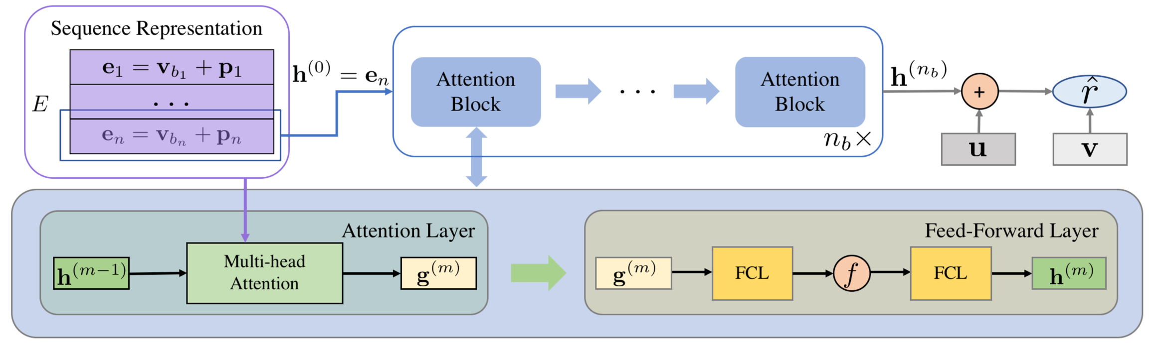
Figure 2. Overall Architecture for $\mathop{\mathtt{RAM}}\limits$

Figure 2 presents the overall architecture of $\mathop{\mathtt{RAM}}\limits$. In $\mathop{\mathtt{RAM}}\limits$, we stack multiple attention blocks with reused item representations to model users’ short-term preferences, and explicitly learn user embeddings to capture long-term preferences. We present the detail of $\mathop{\mathtt{RAM}}\limits$ in the following sections.

5.1. Sequence Representation

Following $\mathop{\mathtt{SASRec}}\limits$, we focus on the most recent $n$ items in users’ interaction histories to generate the recommendations. Specifically, we transform each interaction sequence $S$ to a fixed-length sequence $B$ as presented in Section 4. In $\mathop{\mathtt{RAM}}\limits$, following the literature (Kang and McAuley, 2018; Vaswani et al., 2017), we represent items and positions in each sequence using learnable embeddings. We learn an item embedding matrix $V\in\mathbb{R}^{|\mathbb{V}|\times d}$ in which the $j$-th row $\mathbf{v}_{j}$ is the embedding of item $v_{j}$, and $d$ is the dimension of embeddings. We use a constant zero vector as the embedding of padding items. Similarly, we learn a position embedding matrix $P\in\mathbb{R}^{n\times d}$, and $\mathbf{p}_{t}$ is the embedding of the $t$-th position. Given $V$ and $P$, we represent the sequence $B$ using a matrix $E$ as follows:

(2) $$E=[\mathbf{e}_{1};\mathbf{e}_{2};\cdots;\mathbf{e}_{n}]=[\mathbf{v}_{b_{1}}+\mathbf{p}_{1};\mathbf{v}_{b_{2}}+\mathbf{p}_{2};\cdots;\mathbf{v}_{b_{n}}+\mathbf{p}_{n}],$$

where $\mathbf{e}_{t}=\mathbf{v}_{b_{t}}$+$\mathbf{p}_{t}$ is the $t$-th row in $E$, and $\mathbf{v}_{b_{t}}$ is the embedding of the $t$-th item in $B$.

5.2. Modeling Users’ Short-term Preferences

SA-based methods stack multiple SA blocks to recursively model users’ preferences, and have been demonstrated (Peng et al., 2021; Kang and McAuley, 2018) the state-of-the-art performance in sequential recommendation. Following the idea, in $\mathop{\mathtt{RAM}}\limits$, we also stack multiple attention blocks to model users’ preferences in a recursive manner. In addition, we reuse the item representations in all the attention blocks to mitigate localization deficit. In $\mathop{\mathtt{RAM}}\limits$, we have $n_{b}$ attention blocks, and each attention block contains an attention layer and a feed-forward layer.

5.2.1. Attention layer with reused item embeddings

In the attention layer, we employ the multi-head attention mechanism (Vaswani et al., 2017) to refine the hidden representation of users’ preferences from the previous block as follows:

(3) $$\begin{aligned} \boldsymbol{\beta}^{(m)}_{k}&=\text{softmax}(\frac{(\mathbf{h}^{(m-1)}Q^{(m)}_{k})(EZ^{(m)}_{k})^{\top}}{\sqrt{d}}),\\ \mathbf{head}^{(m)}_{k}&=\boldsymbol{\beta}^{(m)}_{k}(EW^{(m)}_{k}),\\ \mathbf{g}^{(m)}&=[\mathbf{head}^{(m)}_{1},\mathbf{head}^{(m)}_{2},\dots,\mathbf{head}^{(m)}_{n_{h}}]C^{(m)},\\ \end{aligned}$$

where $\mathbf{h}^{(m-1)}$ is the hidden representation of users from the $(m\text{-}1)$-th block, and $\mathbf{g}^{(m)}$ is the output of the attention layer in the $m$-th block. $Q^{(m)}_{k},Z^{(m)}_{k}\text{and }W^{(m)}_{k}\in\mathbb{R}^{d\times\frac{d}{n_{h}}}$ are learnable parameters in the $k$-th head of the attention layer in the $m$-th block, and $C^{(m)}\in\mathbb{R}^{d\times d}$ is also a learnable parameter in the $m$-th block. $\mathbf{head}^{(m)}_{k}$ is the output of the $k$-th head, and $n_{h}$ is the number of heads. Note that as in Equation 3, different from the SA layer in SA-based methods, in $\mathop{\mathtt{RAM}}\limits$, we reuse $E$ in all the attention layers, which could alleviate the effects of cumulating unconcentrated attention weights through blocks. As will be shown in Section 5.5, by doing this, we can also significantly improve the time complexity of computing each attention block from $\mathcal{O}(n^{2}d+nd^{2})$ as in SA to $\mathcal{O}(nd^{2})$, where $d$ is the embedding dimension and $n$ is the length of the fixed-length sequences (i.e., $B$).

5.2.2. Feed-forward layer

Following the literature (Vaswani et al., 2017; Kang and McAuley, 2018; Fan et al., 2022), we include a feed-forward layer after the attention layer to endow $\mathop{\mathtt{RAM}}\limits$ with non-linearity, and better model users’ preferences. Particularly, given $\mathbf{g}^{(m)}$ as in Equation 3, we stack two fully-connected layers (FCLs) as the feed-forward layer as follows:

(4) $$\mathbf{h}^{(m)}=(f(\mathbf{g}^{(m)}W^{(m)}_{1}+\mathbf{b}^{(m)}_{1}))W^{(m)}_{2}+\mathbf{b}^{(m)}_{2},$$

where $f(\cdot)$ is an activation function such as ReLU (Nair and Hinton, 2010) and GELU (Hendrycks and Gimpel, 2016), $W^{(m)}_{1}$, $W^{(m)}_{2}\in\mathbb{R}^{d\times d}$ and $\mathbf{b}^{(m)}_{1}$, $\mathbf{b}^{(m)}_{2}$ are learnable parameters. Following the literature (Kang and McAuley, 2018; Vaswani et al., 2017), we stack attention layers and feed-forward layers using the residual connections (He et al., 2016) to mitigate the degradation problem during the training.

Similarly to that in $\mathop{\mathtt{SASRec}}\limits$, we use $\mathbf{e}_{n}$ (i.e., the representation of the last item in $E$) as the latent representation of users in the first attention block (i.e., $\mathbf{h}^{(0)}=\mathbf{e}_{n}$). Intuitively, $\mathbf{e}_{n}$ consists of embedding the most recently interacted item, and thus, could be viewed as a representation of users’ short-term preferences (Liu et al., 2018; Wu et al., 2019). Conditioned on $\mathbf{e}_{n}$, stacking multiple attention blocks could be viewed as a process to refine the learned representation of users’ short-term preferences, and thus, $\mathbf{h}^{(n_{b})}$ (i.e., the output of the last attention block) could be viewed as the representation of users’ short-term preferences.

5.3. Modeling users’ long-term preferences

As demonstrated in the literature (Peng et al., 2021, 2022), both users’ short-term preferences and long-term preferences play important roles in generating accurate recommendations. However, as discussed in Section 5.2, the attention blocks may focus on learning users’ short-term preferences. As a result, it may not be able to capture users’ long-term preferences fully. To better capture users’ long-term preferences, in $\mathop{\mathtt{RAM}}\limits$, following the literature (Peng et al., 2021; Ma et al., 2019), we explicitly learn user embeddings. Specifically, we learn an embedding matrix $U\in\mathbb{R}^{|\mathbb{U}|\times d}$ in which the $i$-th row $\mathbf{u}_{i}$ is the embedding of user $u_{i}$. Note that, as suggested in the literature (Kang and McAuley, 2018), by considering all the interacted items in each block, SA-based methods (e.g., $\mathop{\mathtt{SASRec}}\limits$) should be able to implicitly learn users’ long-term preferences, and thus, explicitly learning user embeddings may not benefit the performance. In $\mathop{\mathtt{RAM}}\limits$, we also consider all the interacted items in each block. However, as will be shown in Section 7.2, we empirically find that additionally learning user embeddings could significantly improve the recommendation performance on most of the benchmark datasets. In addition, as will be shown in Section 7.2.2, the learned user embeddings and the output from the attention blocks (i.e., $\mathbf{h}^{(n_{b})}$, the representation of user’s short-term preferences) capture different preferences of users, and thus, are complementary for better performance.

5.4. Recommendation Scores and Network Training

Given the output of the attention blocks and the user embeddings, we generate recommendation scores for candidate items as follows:

(5) $$\hat{r}_{ij}=(\mathbf{h}^{(n_{b})}_{i}+\mathbf{u}_{i})\mathbf{v}_{j}^{\top},$$

where $\hat{r}_{ij}$ is the recommendation score of user $u_{i}$ on item $v_{j}$, and $n_{b}$ is the total number of attention blocks in $\mathop{\mathtt{RAM}}\limits$. For each user, we recommend items with the top-$k$ highest recommendation scores. Following $\mathop{\mathtt{SASRec}}\limits$, we employ the binary cross-entropy loss to minimize the negative log-likelihood of correctly recommending the ground truth next item is as follows:

(6) $$\min\limits_{\boldsymbol{\Theta}}-\sum\nolimits_{S_{i}\in T,v_{j}\not\in S_{i}}\log(\sigma(\hat{r}_{ik}))+\log(1-\sigma(\hat{r}_{ij})),$$

where $T$ is the set of all the training sequences, $\boldsymbol{\Theta}$ is the set of learnable parameters (e.g., $V$ and $P$), $v_{k}$ is the ground-truth next item given $S_{i}$. For each training sequence, we randomly generate one negative item $v_{j}$ for the optimization in each epoch. All the learnable parameters are randomly initialized, and are optimized in an end-to-end manner.

5.5. Complexity Analysis

As shown in the literature (Kang and McAuley, 2018), the time complexity for each SA block in SA-based methods is $\mathcal{O}(n^{2}d+nd^{2})$. As a comparison, in $\mathop{\mathtt{RAM}}\limits$, the time complexity of an attention block is only $\mathcal{O}(nd^{2})$, which is theoretically better than that of the SA block. Particularly, computing each SA block requires $6nd^{2}+2n^{2}d+2nd$ operations, while for our attention block, the number of computation operations is only $2nd^{2}+4d^{2}+2nd+2d$, which is also significantly lower than that in SA blocks. As will be shown in Section 7.4, the better time complexity could enable superior runtime performance of $\mathop{\mathtt{RAM}}\limits$ over the SA-based method $\mathop{\mathtt{SASRec}}\limits$ also on modern GPUs.

6. Materials

6.1. Baseline Methods

We compare $\mathop{\mathtt{RAM}}\limits$ with five state-of-the-art baseline methods: 1) $\mathop{\mathtt{Caser}}\limits$ (Tang and Wang, 2018) learns users’ preferences, and the synergies among items using CNNs for sequential recommendation. 2) $\mathop{\mathtt{HAM}}\limits$ (Peng et al., 2021) explicitly models users’ long-term preferences, the high-order and low-order association patterns among items, and the synergies among items to generate recommendations. 3) $\mathop{\mathtt{NARM}}\limits$ (Li et al., 2017) employs RNNs and attention mechanisms to capture both users’ short-term preferences and long-term preferences for the recommendation. 4) $\mathop{\mathtt{HGN}}\limits$ (Ma et al., 2019) leverages attention mechanisms to identify important items and effective latent features for better recommendation. 5) $\mathop{\mathtt{SASRec}}\limits$ (Kang and McAuley, 2018) stacks multiple SA blocks to learn users’ preferences from the interacted items for sequential recommendation. Note that $\mathop{\mathtt{HGN}}\limits$ and $\mathop{\mathtt{SASRec}}\limits$ have been compared with a comprehensive set of other methods including $\mathop{\mathtt{GRU4REC}}\limits$ (Hidasi et al., 2015), $\mathop{\mathtt{GRU4REC\text{++}}}\limits$ (Hidasi and Karatzoglou, 2018) and $\mathop{\mathtt{NextItRec}}\limits$ (Yuan et al., 2019), and have outperformed those methods. Therefore, we compare $\mathop{\mathtt{RAM}}\limits$ with $\mathop{\mathtt{HGN}}\limits$ and $\mathop{\mathtt{SASRec}}\limits$ instead of the methods that they outperform. For all the baseline methods, we use the implementations provided by the authors in GitHub (Section 8).

6.2. Datasets

Table 2. Dataset Statistics

dataset	#users	#items	#intrns	#intrns/u	#u/i
$\mathop{\texttt{Beauty}}\limits$	22,363	12,101	198,502	8.9	16.4
$\mathop{\texttt{Toys}}\limits$	19,412	11,924	167,597	8.6	14.1
$\mathop{\texttt{Children}}\limits$	48,296	32,871	2,784,423	57.6	84.7
$\mathop{\texttt{Comics}}\limits$	34,445	33,121	2,411,314	70.0	72.8
$\mathop{\texttt{ML-1M}}\limits$	6,040	3,952	1,000,209	165.6	253.1
$\mathop{\texttt{ML-20M}}\limits$	129,780	13,663	9,926,480	76.5	726.5

• In this table, “#users”, “#items” and “#intrns” represents the number of users, items and user-item interactions, respectively. The column “#intrns/u” has the average number of interactions of each user. The column “#u/i” has the average number of interactions on each item.

We evaluate the methods on six public benchmark datasets: 1) Amazon-Beauty ($\mathop{\texttt{Beauty}}\limits$) and Amazon-Toys ($\mathop{\texttt{Toys}}\limits$) are from Amazon reviews (Amazon, 2022). These two datasets contain users’ ratings and reviews on beauty products and toys on Amazon, respectively. 2) Goodreads-Children ($\mathop{\texttt{Children}}\limits$) and Goodreads-Comics ($\mathop{\texttt{Comics}}\limits$) are from the goodreads website (GoodReads, 2022), and have users’ ratings and reviews on children and comic books, respectively. 3) MovieLens-1M ($\mathop{\texttt{ML-1M}}\limits$) and MovieLens-20M ($\mathop{\texttt{ML-20M}}\limits$) are from the MovieLens website (MovieLens, 2022), and contain users’ ratings on movies. Following $\mathop{\mathtt{SASRec}}\limits$, for $\mathop{\texttt{Beauty}}\limits$, $\mathop{\texttt{Toys}}\limits$ and $\mathop{\texttt{ML-1M}}\limits$, we only keep the users and items with at least 5 ratings. For $\mathop{\texttt{Children}}\limits$, $\mathop{\texttt{Comics}}\limits$ and $\mathop{\texttt{ML-20M}}\limits$, which are not used in $\mathop{\mathtt{SASRec}}\limits$, following $\mathop{\mathtt{HAM}}\limits$, we keep users with at least 10 ratings, and items with at least 5 ratings. Following the literature (Kang and McAuley, 2018; Peng et al., 2021), we consider the ratings as users’ implicit feedback, and convert ratings into binary values. Particularly, for ratings with a range from 1 to 5, we convert ratings 4 and 5 to binary value 1, or 0 otherwise. Table 2 presents the statistics of the six datasets after the processing.

6.3. Experimental Protocol

6.3.1. Training, validation and testing sets

Following $\mathop{\mathtt{SASRec}}\limits$, on all the datasets, given the historical interactions $S$ of each user, we use the last item (i.e., $s_{|S|}$) in the history for testing, the second last item (i.e., $s_{|S|-1}$) for validation, and all the previous items for training. Also following $\mathop{\mathtt{SASRec}}\limits$, for each training sequence $S$, we extract the last $n$ items $\{b_{1},b_{2},\dots,b_{n}\}$, and split it to $\{b_{1},b_{2}\}$, $\{b_{1},b_{2},b_{3}\}$, $\cdots$, $\{b_{1},b_{2},\dots,b_{n}\}$. We use all the resulted sequences (with necessary padding) for training. We carefully tune the hyper parameters on the validation sets for $\mathop{\mathtt{RAM}}\limits$ and all the baseline methods using grid search, and use the best performing hyper parameters in terms of Recall@$10$ (Section 6.3.2) for testing. To enable a fair comparison, we exhaustively search hyper parameters on a large parameter space. For reproducibility, we report the search range of hyper parameters, and the identified best performing hyper parameters for each method in Section 8.

6.3.2. Evaluation metrics

Following the literature (Kang and McAuley, 2018; Peng et al., 2021; Ma et al., 2019; Tang and Wang, 2018), we use Recall@$k$ and NDCG@$k$ to evaluate $\mathop{\mathtt{RAM}}\limits$ and the baseline methods. Recall@$k$ measures the proportion of sequences in which the ground-truth next item (i.e., $s_{|S|-1}$ during validation and $s_{|S|}$ during testing) is correctly recommended. Particularly, for each sequence, the Recall@$k$ is $1$ if the ground-truth next item is among the top-$k$ of the recommendation list, or $0$ otherwise. NDCG@$k$ is the normalized discounted cumulative gain. It is a widely used rank-aware metric to evaluate the ranking quality of recommendation lists. Following the literature (Kang and McAuley, 2018; Peng et al., 2021; Ma et al., 2019; Tang and Wang, 2018), in our experiments, the gain indicates whether the ground-truth next item is recommended (i.e., gain is $1$) or not (i.e., gain is $0$). In our experiments, we report the average results over all the users for each evaluation metric. For all the evaluation metrics, a higher value indicates better performance.

7. Experimental Results

7.1. Overall Performance

Table 3. Overall Performance

	Dataset	$\mathop{\mathtt{Caser}}\limits$	$\mathop{\mathtt{HAM}}\limits$	$\mathop{\mathtt{NARM}}\limits$	$\mathop{\mathtt{HGN}}\limits$	$\mathop{\mathtt{SASRec}}\limits$	$\mathop{\mathtt{RAM\text{-}u}}\limits$	$\mathop{\mathtt{RAM}}\limits$	impv			$\mathop{\mathtt{Caser}}\limits$	$\mathop{\mathtt{HAM}}\limits$	$\mathop{\mathtt{NARM}}\limits$	$\mathop{\mathtt{HGN}}\limits$	$\mathop{\mathtt{SASRec}}\limits$	$\mathop{\mathtt{RAM\text{-}u}}\limits$	$\mathop{\mathtt{RAM}}\limits$	impv
Recall@10	$\mathop{\texttt{Beauty}}\limits$	0.0647	0.0872	0.0554	0.0782	0.0777	0.0835	$\mathclap{{}^{\dagger~{}}}$0.0888	1.8%		NDCG@10	0.0371	$\mathclap{{}^{\dagger~{}}}$0.0498	0.0291	0.0434	0.0417	0.0460	0.0494	-0.8%
	$\mathop{\texttt{Toys}}\limits$	0.0675	$\mathclap{{}^{\dagger~{}}}$0.1017	0.0557	0.0926	0.0938	0.0998	0.1005	-1.2%			0.0396	$\mathclap{{}^{\dagger~{}}}$0.0617	0.0308	0.0540	0.0525	0.0568	0.0593	-3.9%
	$\mathop{\texttt{Children}}\limits$	0.1303	0.1729	0.1126	0.1536	0.1767	0.1718	$\mathclap{{}^{\dagger~{}}}$0.1906	7.9%			0.0764	0.1038	0.0585	0.0917	0.1083	0.1042	$\mathclap{{}^{\dagger~{}}}$0.1158	6.9%
	$\mathop{\texttt{Comics}}\limits$	0.2320	0.3055	0.1304	0.2857	0.3189	0.3169	$\mathclap{{}^{\dagger~{}}}$0.3286	3.0%			0.1642	0.2319	0.0720	0.2061	0.2433	0.2392	$\mathclap{{}^{\dagger~{}}}$0.2445	0.5%
	$\mathop{\texttt{ML-1M}}\limits$	0.2874	0.2807	0.2349	0.2428	0.2589	0.2732	$\mathclap{{}^{\dagger~{}}}$0.2930	1.9%			$\mathclap{{}^{\dagger~{}}}$0.1619	0.1598	0.1252	0.1374	0.1389	0.1481	0.1612	-0.4%
	$\mathop{\texttt{ML-20M}}\limits$	0.1739	0.1672	OOM	0.1588	0.1892	$\mathclap{{}^{\dagger~{}}}$0.1921	0.1720	1.5%			0.0907	0.0895	OOM	0.0845	0.0979	$\mathclap{{}^{\dagger~{}}}$0.0998	0.0882	1.9%
Recall@20	$\mathop{\texttt{Beauty}}\limits$	0.0869	0.1058	0.0835	0.0978	0.1160	0.1226	$\mathclap{{}^{\dagger~{}}}$0.1291	11.3%		NDCG@20	0.0427	0.0547	0.0362	0.0486	0.0514	0.0558	$\mathclap{{}^{\dagger~{}}}$0.0596	9.0%
	$\mathop{\texttt{Toys}}\limits$	0.0895	0.1182	0.0816	0.1095	0.1292	0.1337	$\mathclap{{}^{\dagger~{}}}$0.1343	3.9%			0.0452	0.0661	0.0373	0.0584	0.0614	0.0654	$\mathclap{{}^{\dagger~{}}}$0.0678	2.6%
	$\mathop{\texttt{Children}}\limits$	0.1832	0.2083	0.1735	0.1854	0.2362	0.2340	$\mathclap{{}^{\dagger~{}}}$0.2573	8.9%			0.0897	0.1131	0.0738	0.1001	0.1233	0.1199	$\mathclap{{}^{\dagger~{}}}$0.1326	7.5%
	$\mathop{\texttt{Comics}}\limits$	0.2791	0.3316	0.1896	0.3122	0.3650	0.3655	$\mathclap{{}^{\dagger~{}}}$0.3822	4.7%			0.1760	0.2388	0.0869	0.2131	0.2549	0.2514	$\mathclap{{}^{\dagger~{}}}$0.2580	1.2%
	$\mathop{\texttt{ML-1M}}\limits$	0.3955	0.3324	0.3422	0.2971	0.3687	0.3891	$\mathclap{{}^{\dagger~{}}}$0.3990	0.9%			$\mathclap{{}^{\dagger~{}}}$0.1892	0.1735	0.1524	0.1518	0.1665	0.1773	0.1880	-0.6%
	$\mathop{\texttt{ML-20M}}\limits$	0.2649	0.2129	OOM	0.2024	0.2908	$\mathclap{{}^{\dagger~{}}}$0.2932	0.2664	0.8%			0.1136	0.1015	OOM	0.0960	0.1234	$\mathclap{{}^{\dagger~{}}}$0.1252	0.1120	1.5%

• For each dataset, the best performance among $\mathop{\mathtt{RAM}}\limits$ and its variant $\mathop{\mathtt{RAM\text{-}u}}\limits$ is in bold, the best performance among the baseline methods is underlined, and the overall best performance is indicated by a dagger (i.e., $\dagger$). The column ”impv” presents the percentage improvement of the best performing variant of $\mathop{\mathtt{RAM}}\limits$ (bold) over the best performing baseline methods (underlined). “OOM” represents the out-of-memory issue.

Table 3 presents the overall performance of $\mathop{\mathtt{RAM}}\limits$, its variant $\mathop{\mathtt{RAM\text{-}u}}\limits$ and the state-of-the-art baseline methods at Recall@$k$ and NDCG@$k$ on six benchmark datasets. In $\mathop{\mathtt{RAM\text{-}u}}\limits$, we remove user embeddings (i.e., $\mathbf{u}_{i}$) when calculating recommendation scores (Equation 5). For $\mathop{\mathtt{NARM}}\limits$, on $\mathop{\texttt{ML-20M}}\limits$, with the implementation provided by the authors, we get the out-of-memory (OOM) issue on NVIDIA Volta V100 GPUs with 16 GB memory.

As shown in Table 3, overall, $\mathop{\mathtt{RAM}}\limits$ is the best performing method on the six datasets. In terms of Recall@$10$, $\mathop{\mathtt{RAM}}\limits$ achieves the best performance on four out of six datasets (i.e., $\mathop{\texttt{Beauty}}\limits$, $\mathop{\texttt{Children}}\limits$, $\mathop{\texttt{Comics}}\limits$ and $\mathop{\texttt{ML-1M}}\limits$), and the second best performance on $\mathop{\texttt{Toys}}\limits$. Similarly, at Recall@$20$, $\mathop{\mathtt{RAM}}\limits$ also significantly outperforms all the baseline methods on five out of six datasets except $\mathop{\texttt{ML-20M}}\limits$. We observe a similar trend at NDCG@$k$. In terms of NDCG@$10$ and NDCG@$20$, $\mathop{\mathtt{RAM}}\limits$ achieves the best or second best performance on five out of six datasets except for $\mathop{\texttt{ML-20M}}\limits$. We notice that on $\mathop{\texttt{ML-20M}}\limits$, compared to the best performing baseline method, the performance of $\mathop{\mathtt{RAM}}\limits$ is considerably worse. However, without user embeddings, $\mathop{\mathtt{RAM\text{-}u}}\limits$ could still achieve the best performance on $\mathop{\texttt{ML-20M}}\limits$. These results demonstrate the strong performance of $\mathop{\mathtt{RAM}}\limits$ and its variant $\mathop{\mathtt{RAM\text{-}u}}\limits$ on different recommendation datasets. It is also worth noting that, different from $\mathop{\mathtt{RAM}}\limits$, $\mathop{\mathtt{Caser}}\limits$ and $\mathop{\mathtt{HAM}}\limits$ do not employ attention mechanisms in learning users’ preferences. As shown in Table 3, compared to $\mathop{\mathtt{Caser}}\limits$, $\mathop{\mathtt{RAM}}\limits$ achieves superior performance on five out of six datasets at Recall@$10$, and all the six datasets at Recall@$20$. Similarly, $\mathop{\mathtt{RAM}}\limits$ also outperforms $\mathop{\mathtt{HAM}}\limits$ on five datasets in terms of Recall@$10$ and all the six datasets in terms of Recall@$20$. These results demonstrate the effectiveness of attention mechanisms for sequential recommendation

7.1.1. Comparison between $\mathop{\mathtt{RAM}}\limits$ and $\mathop{\mathtt{SASRec}}\limits$

The SA-based method $\mathop{\mathtt{SASRec}}\limits$ learns user preferences using stacked SA blocks, and has been demonstrated the state-of-the-art performance in the literature (Peng et al., 2021; Kang and McAuley, 2018). However, as shown in Table 3, $\mathop{\mathtt{RAM}}\limits$ consistently outperforms $\mathop{\mathtt{SASRec}}\limits$ on five out of six datasets (i.e., $\mathop{\texttt{Beauty}}\limits$, $\mathop{\texttt{Toys}}\limits$, $\mathop{\texttt{Children}}\limits$, $\mathop{\texttt{Comics}}\limits$ and $\mathop{\texttt{ML-1M}}\limits$). Particularly, compared to $\mathop{\mathtt{SASRec}}\limits$, in terms of Recall@$10$, $\mathop{\mathtt{RAM}}\limits$ achieves a significant improvement of 9.1%, on average, over the five datasets. In terms of NDCG@$10$, $\mathop{\mathtt{RAM}}\limits$ also significantly outperforms $\mathop{\mathtt{SASRec}}\limits$ with an average improvement of 11.0% over the five datasets. On $\mathop{\texttt{ML-20M}}\limits$, although the performance of $\mathop{\mathtt{RAM}}\limits$ is worse than that of $\mathop{\mathtt{SASRec}}\limits$, $\mathop{\mathtt{RAM\text{-}u}}\limits$ could still outperform $\mathop{\mathtt{SASRec}}\limits$ by a considerable margin. $\mathop{\mathtt{SASRec}}\limits$ recursively aggregates and updates item representations through stacked SA blocks to capture both users’ short-term and long-term preferences. However, as discussed in Section 4, the learned attention maps in $\mathop{\mathtt{SASRec}}\limits$ could suffer from the localization-deficit issue, and thus, in each block, updating the item representations based on the attention map could induce a dramatic change in the item representations over blocks, and eventually impair the recommendation performance. Differently from $\mathop{\mathtt{SASRec}}\limits$, in $\mathop{\mathtt{RAM}}\limits$, we reuse item representations through blocks to mitigate the issue, and also explicitly learn user embeddings to capture users’ long-term preferences. Therefore, $\mathop{\mathtt{RAM}}\limits$ could enable substantially better recommendation performance over $\mathop{\mathtt{SASRec}}\limits$ on the benchmark datasets.

7.1.2. Comparison between $\mathop{\mathtt{RAM}}\limits$ and $\mathop{\mathtt{HGN}}\limits$

Table 3 also shows that overall $\mathop{\mathtt{RAM}}\limits$ substantially outperforms $\mathop{\mathtt{HGN}}\limits$ on all the six benchmark datasets. For example, in terms of Recall@$10$ and Recall@$20$, $\mathop{\mathtt{RAM}}\limits$ achieves significant improvement over $\mathop{\mathtt{HGN}}\limits$ on all the six datasets. On average, compared to $\mathop{\mathtt{HGN}}\limits$, $\mathop{\mathtt{RAM}}\limits$ achieves a substantial improvement of 15.0% and 30.3% at Recall@$10$ and Recall@$20$, respectively. Similarly to $\mathop{\mathtt{RAM}}\limits$, $\mathop{\mathtt{HGN}}\limits$ also learns attention weights to aggregate items and capture users’ preferences. However, $\mathop{\mathtt{HGN}}\limits$ directly learns users’ preferences using one attention layer, while $\mathop{\mathtt{RAM}}\limits$ stacks multiple attention-blocks to model users’ preferences recursively. Given the complex nature of users’ preferences (Yakhchi, 2021), one layer may not be sufficient to fully capture users’ preferences. Therefore, by recursively modeling users’ preferences via multiple blocks, $\mathop{\mathtt{RAM}}\limits$ could achieve superior recommendation performance over $\mathop{\mathtt{HGN}}\limits$ on all the six benchmark datasets. Note that in $\mathop{\mathtt{HGN}}\limits$, there is no mechanism to stack multiple layers, and thus, it could be non-trivial to extend $\mathop{\mathtt{HGN}}\limits$ to a multi-layer version.

7.1.3. Comparison between $\mathop{\mathtt{RAM}}\limits$ and $\mathop{\mathtt{NARM}}\limits$

Table 3 shows that compared to the RNNs-based method $\mathop{\mathtt{NARM}}\limits$, $\mathop{\mathtt{RAM}}\limits$ demonstrates superior performance on all the six datasets at all the evaluation metrics. $\mathop{\mathtt{NARM}}\limits$ primarily uses RNNs to recurrently learn users’ preferences. As shown in the literature (Vaswani et al., 2017), due to the recurrent nature, RNNs may not be effective in modeling long-range dependencies in the sequence. In $\mathop{\mathtt{RAM}}\limits$, similarly to that in SA-based methods, we use attention mechanisms to model users’ preferences, which could be more effective than RNNs in capturing the long-range dependencies as demonstrated in the literature (Vaswani et al., 2017). Therefore $\mathop{\mathtt{RAM}}\limits$ could significantly outperform RNNs-based method $\mathop{\mathtt{NARM}}\limits$ on benchmark datasets.

7.2. User Embedding Analysis

We conduct an analysis to verify the importance of learning user embeddings in $\mathop{\mathtt{RAM}}\limits$. Specifically, we compare the performance of $\mathop{\mathtt{RAM}}\limits$ and its variant $\mathop{\mathtt{RAM\text{-}u}}\limits$ to verify the effectiveness of user embeddings. We also investigate the similarities between the representation of users’ short-term preferences and the user embeddings to verify if they capture different preferences of users.

7.2.1. Effectiveness of user embeddings

As shown in Table 3, without user embeddings, the performance of $\mathop{\mathtt{RAM\text{-}u}}\limits$ drops significantly on five out six datasets except for $\mathop{\texttt{ML-20M}}\limits$. For example, in terms of Recall@10, on $\mathop{\texttt{Children}}\limits$ and $\mathop{\texttt{Comics}}\limits$, $\mathop{\mathtt{RAM\text{-}u}}\limits$ underperforms $\mathop{\mathtt{RAM}}\limits$ at 9.9% and 3.6%, respectively. On average. over the five datasets, $\mathop{\mathtt{RAM\text{-}u}}\limits$ underperforms $\mathop{\mathtt{RAM}}\limits$ at 5.3% in Recall@10. In $\mathop{\mathtt{RAM}}\limits$, we hypothesize that the attention blocks may not be able to effectively capture users’ long-term preferences. Therefore, following the literature (Peng et al., 2021; Ma et al., 2019), we explicitly learn user embeddings to better capture the long-term preferences in the model. These results demonstrate the importance of separately modeling users’ short-term preferences and long-term preferences for sequential recommendation. We notice that on $\mathop{\texttt{ML-20M}}\limits$, different from that in the other datasets, including user embeddings results in worse performance. This might be due to the reason that in some datasets, users’ interactions primarily depend on their short-term preferences (Liu et al., 2018), and thus, incorporating the long-term preferences when generating the recommendations may not benefit the performance.

7.2.2. Similarities between the representation of users’ short-term preferences and user embeddings

In $\mathop{\mathtt{RAM}}\limits$, as discussed in Section 5.3, we view the outputs from the attention blocks (i.e., $\mathbf{h}_{i}^{(n_{b})}$) as the representations of users’ short-term preferences, and combine them with the user embeddings (i.e., $\mathbf{u}_{i}$) for the recommendation. Intuitively, users’ short-term and long-term preferences might be different, and thus, combining both $\mathbf{h}_{i}^{(n_{b})}$ and $\mathbf{u}_{i}$ could enable better performance. To verify this, we calculate the cosine similarities between $\mathbf{h}_{i}^{(n_{b})}$ and $\mathbf{u}_{i}$. For each user $u_{i}$, we also randomly sample another user $u_{j}$ and calculate the cosine similarity between $\mathbf{h}_{i}^{(n_{b})}$ and $\mathbf{u}_{j}$. Generally, the short-term preferences and long-term preferences from two different users should be considerably different, and can be used as a baseline to evaluate those from the same user.

(a) $\mathop{\texttt{Beauty}}\limits$

(b) $\mathop{\texttt{Toys}}\limits$

(c) $\mathop{\texttt{Children}}\limits$

(d) $\mathop{\texttt{Comics}}\limits$

(e) $\mathop{\texttt{ML-1M}}\limits$

(f) $\mathop{\texttt{ML-20M}}\limits$

Figure 3. Cosine Similarities Between the representation of users’ short-term and long-term preferences

Figure 3 presents the distribution of the cosine similarities between the preference representations from the same user (i.e., $\mathbf{h}_{i}^{(n_{b})}$ and $\mathbf{u}_{i}$), and different users (i.e., $\mathbf{h}_{i}^{(n_{b})}$ and $\mathbf{u}_{j}$) on the six benchmark datasets. As shown in Figure 3, on all the datasets, the distribution of the similarities between $\mathbf{h}_{i}^{(n_{b})}$ and $\mathbf{u}_{i}$ is close to that between $\mathbf{h}_{i}^{(n_{b})}$ and $\mathbf{u}_{j}$. Recall that since from different users, $\mathbf{h}_{i}^{(n_{b})}$ and $\mathbf{u}_{j}$ should generally represent different preferences. Therefore, these results reveal that $\mathbf{h}_{i}^{(n_{b})}$ and $\mathbf{u}_{i}$ capture different preferences of users, and thus, as shown in Table 3, using both of them for the recommendation could significantly improve the performance on most of the datasets.

7.3. Stability Analysis

We also analyze to evaluate the stability of $\mathop{\mathtt{SASRec}}\limits$ and $\mathop{\mathtt{RAM}}\limits$ on learning deep and wide models. Following the literature (Cheng et al., 2016), we use the number of blocks (i.e., $n_{b}$) and the embedding dimensions (i.e., $d$) to represent the depth and width of models, respectively. To enable a fair comparison, in this analysis, we also compare $\mathop{\mathtt{SASRec}}\limits$ with $\mathop{\mathtt{RAM\text{-}u}}\limits$ to eliminate the effects of user embeddings. We use the identified best-performing hyper parameters on $\mathop{\mathtt{SASRec}}\limits$ for $\mathop{\mathtt{SASRec}}\limits$, $\mathop{\mathtt{RAM\text{-}u}}\limits$ and $\mathop{\mathtt{RAM}}\limits$, and study how $d$ and $n_{b}$ affect the performance.

7.3.1. Stability over the number of blocks

Figure 4 presents the performance of $\mathop{\mathtt{SASRec}}\limits$, $\mathop{\mathtt{RAM\text{-}u}}\limits$ and $\mathop{\mathtt{RAM}}\limits$ over the different number of blocks on the six benchmark datasets. On $\mathop{\texttt{ML-20M}}\limits$, we have the out-of-memory issue on $\mathop{\mathtt{SASRec}}\limits$ when $n_{b}>6$. Thus, on $\mathop{\texttt{ML-20M}}\limits$, we only report the performance of $\mathop{\mathtt{SASRec}}\limits$ when $n_{b}\leq 6$.

(a) $\mathop{\texttt{Beauty}}\limits$

(b) $\mathop{\texttt{Toys}}\limits$

(c) $\mathop{\texttt{Children}}\limits$

(d) $\mathop{\texttt{Comics}}\limits$

(e) $\mathop{\texttt{ML-1M}}\limits$

(f) $\mathop{\texttt{ML-20M}}\limits$

Figure 4. Performance over a different number of blocks

As shown in Figure 4, both $\mathop{\mathtt{RAM\text{-}u}}\limits$ and $\mathop{\mathtt{RAM}}\limits$ are more stable than $\mathop{\mathtt{SASRec}}\limits$ on learning deep models. Particularly, for $\mathop{\mathtt{RAM\text{-}u}}\limits$ and $\mathop{\mathtt{RAM}}\limits$, on all the datasets, they could perform reasonably well when the model is very deep (e.g., $n_{b}=8$). However, for $\mathop{\mathtt{SASRec}}\limits$, on $\mathop{\texttt{Beauty}}\limits$ and $\mathop{\texttt{Toys}}\limits$, the performance drops dramatically when the number of blocks (i.e., $n_{b}$) is larger than seven. In $\mathop{\texttt{Children}}\limits$ and $\mathop{\texttt{Comics}}\limits$, the performance also degrades dramatically when $n_{b}>4$ and $n_{b}>5$, respectively. Moreover, on $\mathop{\texttt{ML-1M}}\limits$ and $\mathop{\texttt{ML-20M}}\limits$, $\mathop{\mathtt{SASRec}}\limits$ performs very poorly when $n_{b}>3$. As discussed in Section 5.2.1, the attention maps learned in $\mathop{\mathtt{SASRec}}\limits$ could suffer from the localization-deficit issue. As a consequence, in the lower blocks, the item representations updated with the localization-deficit attention maps could change dramatically, and further impair the localization of the following maps. Through multiple blocks, this problem could be amplified, and thus, $\mathop{\mathtt{SASRec}}\limits$ could be unstable on learning deep models. Different from $\mathop{\mathtt{SASRec}}\limits$, in $\mathop{\mathtt{RAM\text{-}u}}\limits$ and $\mathop{\mathtt{RAM}}\limits$, we do not update the item representations, and reuse them through all the blocks to avoid this issue. Therefore, $\mathop{\mathtt{RAM\text{-}u}}\limits$ and $\mathop{\mathtt{RAM}}\limits$ could learn deeper models than $\mathop{\mathtt{SASRec}}\limits$ for better performance. We notice that on $\mathop{\texttt{Toys}}\limits$, the performance of $\mathop{\mathtt{RAM\text{-}u}}\limits$ and $\mathop{\mathtt{RAM}}\limits$ drop considerably when $n_{b}>6$. As shown in Table 2, $\mathop{\texttt{Toys}}\limits$ is the most sparse dataset in our experiments. As a result, the sparse interactions in $\mathop{\texttt{Toys}}\limits$ may not enable learning very deep models. However, on $\mathop{\texttt{Toys}}\limits$, $\mathop{\mathtt{RAM\text{-}u}}\limits$ and $\mathop{\mathtt{RAM}}\limits$ could still outperform $\mathop{\mathtt{SASRec}}\limits$ when $n_{b}=8$. It is also worth noting that, as will be shown in Section 8, on $\mathop{\texttt{Toys}}\limits$, $\mathop{\texttt{ML-1M}}\limits$ and $\mathop{\texttt{ML-20M}}\limits$, the best performing $\mathop{\mathtt{RAM\text{-}u}}\limits$ and $\mathop{\mathtt{RAM}}\limits$ have at least 4 blocks, which reveals that on specific datasets, learning moderately deep models could benefit the performance.

We also investigate the output (i.e., $\mathbf{h}^{(m)}$) from each attention block of $\mathop{\mathtt{SASRec}}\limits$ and $\mathop{\mathtt{RAM}}\limits$ to better understand why $\mathop{\mathtt{RAM}}\limits$ could be more stable than $\mathop{\mathtt{SASRec}}\limits$ in learning deep models. Intuitively, to ensure stability, the outputs of consecutive attention blocks should not change significantly. To verify this, we calculate the cosine similarity between the outputs of consecutive attention blocks (i.e., sim($h^{(m)}$, $h^{(m+1)}$)). Specifically, we use the best-performing hyper parameters (Section 8) for $\mathop{\mathtt{SASRec}}\limits$ and $\mathop{\mathtt{RAM}}\limits$, and export the outputs over attention blocks to calculate their similarities. We find that the cosine similarity between $h^{(m)}$ and $h^{(m+1)}$ in $\mathop{\mathtt{RAM}}\limits$ is considerably higher than that in $\mathop{\mathtt{SASRec}}\limits$. For example, on $\mathop{\texttt{ML-1M}}\limits$, in $\mathop{\mathtt{RAM}}\limits$, sim($h^{(1)}$, $h^{(2)}$), and sim($h^{(2)}$, $h^{(3)}$) is $0.819$ and $0.797$, respectively. However, for $\mathop{\mathtt{SASRec}}\limits$, sim($h^{(1)}$, $h^{(2)}$) and sim($h^{(2)}$, $h^{(3)}$) are both $0.719$. The higher similarities in $\mathop{\mathtt{RAM}}\limits$ over $\mathop{\mathtt{SASRec}}\limits$ indicate that in $\mathop{\mathtt{RAM}}\limits$, the outputs over blocks are more consistent compared to those in $\mathop{\mathtt{SASRec}}\limits$, and thus, could enable better stability.

7.3.2. Stability over embedding dimensions

Figure 5 presents the performance of $\mathop{\mathtt{SASRec}}\limits$, $\mathop{\mathtt{RAM\text{-}u}}\limits$ and $\mathop{\mathtt{RAM}}\limits$ over different embedding dimensions on the six datasets. On $\mathop{\texttt{ML-20M}}\limits$, when $d=2048$, for all the three methods, we cannot finish the training within 48 hours. Thus, on $\mathop{\texttt{ML-20M}}\limits$, we only report the results when $d<2048$.

(a) $\mathop{\texttt{Beauty}}\limits$

(b) $\mathop{\texttt{Toys}}\limits$

(c) $\mathop{\texttt{Children}}\limits$

(d) $\mathop{\texttt{Comics}}\limits$

(e) $\mathop{\texttt{ML-1M}}\limits$

(f) $\mathop{\texttt{ML-20M}}\limits$

Figure 5. Performance over different embedding dimensions

As shown in Figure 5, overall, $\mathop{\mathtt{RAM\text{-}u}}\limits$ and $\mathop{\mathtt{RAM}}\limits$ are also more stable than $\mathop{\mathtt{SASRec}}\limits$ on learning wide models. On all the datasets, both $\mathop{\mathtt{RAM\text{-}u}}\limits$ and $\mathop{\mathtt{RAM}}\limits$ could perform reasonably well when the model is very wide (i.e., $d$ is $1024$ or $2048$). However, for $\mathop{\mathtt{SASRec}}\limits$, on $\mathop{\texttt{Beauty}}\limits$ and $\mathop{\texttt{Toys}}\limits$, the performance drops dramatically when the embedding dimension is larger than $1024$ and $512$, respectively. Similarly, on $\mathop{\texttt{ML-1M}}\limits$ and $\mathop{\texttt{ML-20M}}\limits$, $\mathop{\mathtt{SASRec}}\limits$ also performs poorly when $d>256$. These results demonstrate that reusing item representations could also enable $\mathop{\mathtt{RAM\text{-}u}}\limits$ and $\mathop{\mathtt{RAM}}\limits$ to learn wider models than $\mathop{\mathtt{SASRec}}\limits$ for better performance. We notice that on $\mathop{\texttt{Children}}\limits$ and $\mathop{\texttt{Comics}}\limits$, $\mathop{\mathtt{SASRec}}\limits$ could achieve reasonable performance when $d$ is very large (i.e., $2048$). However, on these datasets, when $d=2048$, $\mathop{\mathtt{RAM\text{-}u}}\limits$ and $\mathop{\mathtt{RAM}}\limits$ could still outperform $\mathop{\mathtt{SASRec}}\limits$ by a considerable margin, indicating the capability of $\mathop{\mathtt{RAM\text{-}u}}\limits$ and $\mathop{\mathtt{RAM}}\limits$ in learning wide models.

7.4. Run-time Performance over the Number of Attention Blocks

We conduct an analysis to evaluate the run-time performance of $\mathop{\mathtt{RAM}}\limits$ and $\mathop{\mathtt{SASRec}}\limits$ during testing. Similarly to that in Section 7.3.1, we apply the best performing hyper parameters on $\mathop{\mathtt{SASRec}}\limits$ for $\mathop{\mathtt{SASRec}}\limits$ and $\mathop{\mathtt{RAM}}\limits$, and study their run-time performance during testing over the different number of attention blocks. To enable a fair comparison, we perform the evaluation for both $\mathop{\mathtt{SASRec}}\limits$ and $\mathop{\mathtt{RAM}}\limits$ using NVIDIA Volta V100 GPUs, and report the average computation time per user over five runs in Figure 6. We focus on the run-time performance during testing due to the fact that it could signify the models’ latency in real-time recommendation, that could significantly affect the user experience and thus revenue.

(a) $\mathop{\texttt{Beauty}}\limits$

(b) $\mathop{\texttt{Toys}}\limits$

(c) $\mathop{\texttt{Children}}\limits$

(d) $\mathop{\texttt{Comics}}\limits$

(e) $\mathop{\texttt{ML-1M}}\limits$

(f) $\mathop{\texttt{ML-20M}}\limits$

Figure 6. Runtime Performance over Different Number of Layers

As shown in Figure 6, on all the datasets, $\mathop{\mathtt{RAM}}\limits$ has better run-time performance than $\mathop{\mathtt{SASRec}}\limits$ over all the blocks, and the improvement increases as the number of blocks increases. Particularly, when $n_{b}$ is the best performing one for $\mathop{\mathtt{SASRec}}\limits$ on each dataset (e.g., $n_{b}=2$ on $\mathop{\texttt{Beauty}}\limits$ as in Section 8), in terms of the run-time performance, $\mathop{\mathtt{RAM}}\limits$ could achieve a 16.6% speedup over $\mathop{\mathtt{SASRec}}\limits$ on the six datasets. As shown in Figure 4, with the same hyper parameters, on all the datasets except $\mathop{\texttt{ML-20M}}\limits$, $\mathop{\mathtt{RAM}}\limits$ could also outperform $\mathop{\mathtt{SASRec}}\limits$ in terms of the recommendation performance. These results demonstrate that compared to $\mathop{\mathtt{SASRec}}\limits$, $\mathop{\mathtt{RAM}}\limits$ could generate more satisfactory recommendations in lower latency, and thus, could significantly improve the user experience. Note that on GPUs, all the computations are performed parallelly. However, when calculating the time complexity (Section 5.5), we assume the computations are serial. Therefore, in terms of the run-time performance on modern GPUs, the improvement of $\mathop{\mathtt{RAM}}\limits$ over $\mathop{\mathtt{SASRec}}\limits$ may not be as significant as that on theoretical time complexity. However, in many applications, the recommendation model could be deployed on edge devices with limited computing resources. In these applications, as suggested by the time complexity comparison (Section 5.5), $\mathop{\mathtt{RAM}}\limits$ could achieve more substantial speedup over $\mathop{\mathtt{SASRec}}\limits$.

8. Reproducibility

Table 4. Hyper Parameters for $\mathop{\mathtt{RAM}}\limits$, $\mathop{\mathtt{RAM\text{-}u}}\limits$ and Baseline Methods

Dataset	$\mathop{\mathtt{Caser}}\limits$						$\mathop{\mathtt{HAM}}\limits$							$\mathop{\mathtt{NARM}}\limits$			$\mathop{\mathtt{HGN}}\limits$					$\mathop{\mathtt{SASRec}}\limits$					$\mathop{\mathtt{RAM\text{-}u}}\limits$					$\mathop{\mathtt{RAM}}\limits$
	$d$	$n_{s}$	$n_{p}$	$n_{v}$	$n_{f}$		$d$	$n_{s}$	$n_{p}$	$\lambda$	$n_{l}$	$n_{o}$		$d$	$l_{r}$		$d$	$n_{s}$	$n_{p}$	$\lambda$		$d$	$n$	$n_{h}$	$n_{b}$		$d$	$n$	$n_{h}$	$n_{b}$		$d$	$n$	$n_{h}$	$n_{b}$
$\mathop{\texttt{Beauty}}\limits$	512	4	1	2	8		512	3	2	1e-3	1	1		512	1e-3		512	3	2	1e-3		128	75	4	2		256	75	4	2		256	75	16	3
$\mathop{\texttt{Toys}}\limits$	512	4	1	1	4		512	3	1	1e-3	1	1		512	1e-3		512	3	1	1e-4		128	50	2	3		256	50	4	4		256	50	8	4
$\mathop{\texttt{Children}}\limits$	512	4	1	2	4		256	4	2	1e-4	1	2		256	1e-4		256	3	1	0		256	175	2	1		256	200	1	2		512	100	1	1
$\mathop{\texttt{Comics}}\limits$	512	4	1	1	4		512	3	1	0	1	3		256	1e-3		512	3	1	0		256	200	1	1		512	200	1	1		512	200	1	1
$\mathop{\texttt{ML-1M}}\limits$	128	6	1	4	16		512	5	1	1e-3	2	1		512	1e-4		128	4	1	1e-3		256	150	4	3		512	200	2	5		512	200	4	4
$\mathop{\texttt{ML-20M}}\limits$	256	6	1	2	8		256	5	2	1e-3	3	3		OOM	OOM		128	4	2	1e-3		256	150	2	3		512	150	8	5		256	100	4	4

• This table presents the best performing hyper parameters of all the methods on the six benchmark datasets. In the table. “OOM” represents the out of memory issue.

We implement $\mathop{\mathtt{RAM}}\limits$ in python 3.7.11 with PyTorch 1.10.2 . We use Adam optimizer with learning rate 1e-3 for $\mathop{\mathtt{RAM}}\limits$ on all the datasets. The source code and processed data are available on Google Drive . For $\mathop{\mathtt{SASRec}}\limits$, $\mathop{\mathtt{RAM\text{-}u}}\limits$ and $\mathop{\mathtt{RAM}}\limits$, we search the embedding dimension $d$ in $\{64,128,256,512\}$, the length of the fixed-length sequences $n$ in $\{50,75,100,125,150,175,200\}$, the number of heads $n_{h}$ in $\{1,2,4,8,16\}$, and the number of blocks $n_{b}$ in $\{1,2,3,4,5\}$. We use GELU (Hendrycks and Gimpel, 2016) as the activation function in the feed-forward layer for all the three methods. We use the PyTorch implementation in GitHub (pmixer, 2022) for $\mathop{\mathtt{SASRec}}\limits$. For $\mathop{\mathtt{HGN}}\limits$ (Ma, 2022), we search $d$ in $\{64,128,256,512\}$, the length of the subsequences $n_{s}$ in $\{3,4,5\}$, the number of items $n_{p}$ to calculate recommendation errors during training in $\{1,2\}$, and the regularization factor $\lambda$ in {0, 1e-3, 1e-4}. For $\mathop{\mathtt{NARM}}\limits$ (Li, 2022), we search $d$ in $\{64,128,256,512\}$ and the learning rate $l_{r}$ in {1e-2, 1e-3, 1e-4}. For $\mathop{\mathtt{HAM}}\limits$ (Peng, 2022), we search $d$ in $\{64,128,256,512\}$, $n_{s}$ in $\{3,4,5\}$, $n_{p}$ in $\{1,2\}$, $\lambda$ in {0, 1e-3, 1e-4}, the number of items in low order $n_{l}$ in $\{1,2,3\}$, and the order of item synergies $n_{o}$ in $\{1,2,3\}$. For $\mathop{\mathtt{Caser}}\limits$ (Tang, 2022), we search $d$ in $\{64,128,256,512\}$, $n_{s}$ in $\{4,5,6\}$, $n_{p}$ in $\{1,2\}$, the number of vertical filters in CNNs $n_{v}$ in $\{1,2,4\}$, and the number of horizontal filters in CNNs $n_{f}$ in $\{4,8,16\}$. We report the best performing hyper parameters from the validation set in Table 4.

9. Conclusion

In this manuscript, we identified the localization-deficit issue in SA-based sequential recommendation methods. To mitigate the effects of this issue and improve the recommendation performance, we reused item representations throughout all the attention blocks and developed the novel method $\mathop{\mathtt{RAM}}\limits$ for sequential recommendation. $\mathop{\mathtt{RAM}}\limits$ models users’ short-term preferences using the attention blocks with feed-forward layers, and also users’ long-term preferences explicitly using a user embedding. We also developed a variant of $\mathop{\mathtt{RAM}}\limits$ with the user embedding removed. We extensively evaluated $\mathop{\mathtt{RAM}}\limits$ and $\mathop{\mathtt{RAM\text{-}u}}\limits$ against five state-of-the-art baseline methods $\mathop{\mathtt{Caser}}\limits$, $\mathop{\mathtt{HAM}}\limits$, $\mathop{\mathtt{NARM}}\limits$, $\mathop{\mathtt{HGN}}\limits$ and $\mathop{\mathtt{SASRec}}\limits$ on six benchmark datasets $\mathop{\texttt{Beauty}}\limits$, $\mathop{\texttt{Toys}}\limits$, $\mathop{\texttt{Children}}\limits$, $\mathop{\texttt{Comics}}\limits$, $\mathop{\texttt{ML-1M}}\limits$ and $\mathop{\texttt{ML-20M}}\limits$. Our experimental results show that $\mathop{\mathtt{RAM}}\limits$ and $\mathop{\mathtt{RAM\text{-}u}}\limits$ can achieve superior performance over the baseline methods on benchmark datasets, with an improvement of up to 11.3%. Our experiments also show that explicitly learning and integrating users’ long-term preferences can benefit $\mathop{\mathtt{RAM}}\limits$. In addition, $\mathop{\mathtt{RAM}}\limits$ shows better stability in learning deep and wide models than the baseline methods. In terms of run-time performance, we also observed that $\mathop{\mathtt{RAM}}\limits$ is more efficient than the baselines, and thus has a great potential to be applied in systems with limited computing resources.

References

- (1)
- Amazon (2022) Amazon. last visited at 2022. Amazon review dataset. {http://jmcauley.ucsd.edu/data/amazon/}.
- Bahdanau et al. (2014) Dzmitry Bahdanau, Kyunghyun Cho, and Yoshua Bengio. 2014. Neural machine translation by jointly learning to align and translate. arXiv preprint arXiv:1409.0473 (2014).
- Belletti et al. (2019) Francois Belletti, Minmin Chen, and Ed H Chi. 2019. Quantifying long range dependence in language and user behavior to improve rnns. In Proceedings of the 25th ACM SIGKDD International Conference on Knowledge Discovery & Data Mining. 1317–1327.
- Cheng et al. (2016) Heng-Tze Cheng, Levent Koc, Jeremiah Harmsen, Tal Shaked, Tushar Chandra, Hrishi Aradhye, Glen Anderson, Greg Corrado, Wei Chai, Mustafa Ispir, et al. 2016. Wide & deep learning for recommender systems. In Proceedings of the 1st workshop on deep learning for recommender systems. 7–10.
- Fan et al. (2022) Ziwei Fan, Zhiwei Liu, Yu Wang, Alice Wang, Zahra Nazari, Lei Zheng, Hao Peng, and Philip S Yu. 2022. Sequential Recommendation via Stochastic Self-Attention. arXiv preprint arXiv:2201.06035 (2022).
- GoodReads (2022) GoodReads. last visited at 2022. GoodReads dataset. https://www.goodreads.com/.
- Hart (1971) P. E. Hart. 1971. Entropy and Other Measures of Concentration. Journal of the Royal Statistical Society. Series A (General) 134, 1 (1971), 73–85. http://www.jstor.org/stable/2343975
- He et al. (2016) Kaiming He, Xiangyu Zhang, Shaoqing Ren, and Jian Sun. 2016. Deep residual learning for image recognition. In Proceedings of the IEEE conference on computer vision and pattern recognition. 770–778.
- He and McAuley (2016) Ruining He and Julian McAuley. 2016. Ups and downs: Modeling the visual evolution of fashion trends with one-class collaborative filtering. In proceedings of the 25th international conference on world wide web. 507–517.
- Hendrycks and Gimpel (2016) Dan Hendrycks and Kevin Gimpel. 2016. Gaussian error linear units (gelus). arXiv preprint arXiv:1606.08415 (2016).
- Hidasi and Karatzoglou (2018) Balázs Hidasi and Alexandros Karatzoglou. 2018. Recurrent neural networks with top-k gains for session-based recommendations. In Proceedings of the 27th ACM international conference on information and knowledge management. 843–852.
- Hidasi et al. (2015) Balázs Hidasi, Alexandros Karatzoglou, Linas Baltrunas, and Domonkos Tikk. 2015. Session-based recommendations with recurrent neural networks. arXiv preprint arXiv:1511.06939 (2015).
- Kang and McAuley (2018) Wang-Cheng Kang and Julian McAuley. 2018. Self-attentive sequential recommendation. In 2018 IEEE International Conference on Data Mining (ICDM). IEEE, 197–206.
- Li (2022) Jing Li. last visited at 2022. PyTorch implementation for NARM. https://github.com/Wang-Shuo/Neural-Attentive-Session-Based-Recommendation-PyTorch.
- Li et al. (2017) Jing Li, Pengjie Ren, Zhumin Chen, Zhaochun Ren, Tao Lian, and Jun Ma. 2017. Neural attentive session-based recommendation. In Proceedings of the 2017 ACM on Conference on Information and Knowledge Management. 1419–1428.
- Liu et al. (2018) Qiao Liu, Yifu Zeng, Refuoe Mokhosi, and Haibin Zhang. 2018. STAMP: Short-Term Attention/Memory Priority Model for Session-Based Recommendation. In Proceedings of the 24th ACM SIGKDD International Conference on Knowledge Discovery and Data Mining. Association for Computing Machinery, New York, NY, USA.
- Ma (2022) Chen Ma. last visited at 2022. PyTorch implementation for HGN. https://github.com/allenjack/HGN.
- Ma et al. (2019) Chen Ma, Peng Kang, and Xue Liu. 2019. Hierarchical gating networks for sequential recommendation. In Proceedings of the 25th ACM SIGKDD international conference on knowledge discovery & data mining. 825–833.
- McAuley et al. (2015) Julian McAuley, Christopher Targett, Qinfeng Shi, and Anton Van Den Hengel. 2015. Image-based recommendations on styles and substitutes. In Proceedings of the 38th international ACM SIGIR conference on research and development in information retrieval. 43–52.
- Mikolov et al. (2013) Tomas Mikolov, Ilya Sutskever, Kai Chen, Greg S Corrado, and Jeff Dean. 2013. Distributed representations of words and phrases and their compositionality. Advances in neural information processing systems 26 (2013).
- MovieLens (2022) MovieLens. last visited at 2022. MovieLens dataset. https://movielens.org/.
- Nair and Hinton (2010) Vinod Nair and Geoffrey E Hinton. 2010. Rectified linear units improve restricted boltzmann machines. In Icml.
- Peng (2022) Bo Peng. last visited at 2022. PyTorch implementation for HAM. https://github.com/BoPeng112/HAM.
- Peng et al. (2021) Bo Peng, Zhiyun Ren, Srinivasan Parthasarathy, and Xia Ning. 2021. HAM: hybrid associations models for sequential recommendation. IEEE Transactions on Knowledge and Data Engineering (2021).
- Peng et al. (2022) Bo Peng, Zhiyun Ren, Srinivasan Parthasarathy, and Xia Ning. 2022. M2: Mixed Models with Preferences, Popularities and Transitions for Next-Basket Recommendation. IEEE Transactions on Knowledge and Data Engineering (2022), 1–1. https://doi.org/10.1109/tkde.2022.3142773
- pmixer (2022) pmixer. last visited at 2022. PyTorch implementation for SASRec. https://github.com/pmixer/SASRec.pytorch.
- Shim et al. (2021) Kyuhong Shim, Jungwook Choi, and Wonyong Sung. 2021. Understanding the role of self attention for efficient speech recognition. In International Conference on Learning Representations.
- Tang (2022) Jiaxi Tang. last visited at 2022. PyTorch implementation for Caser. https://github.com/graytowne/caser_pytorch.
- Tang and Wang (2018) Jiaxi Tang and Ke Wang. 2018. Personalized top-n sequential recommendation via convolutional sequence embedding. In Proceedings of the eleventh ACM international conference on web search and data mining. 565–573.
- Tay et al. (2021) Yi Tay, Dara Bahri, Donald Metzler, Da-Cheng Juan, Zhe Zhao, and Che Zheng. 2021. Synthesizer: Rethinking self-attention for transformer models. In International Conference on Machine Learning. PMLR, 10183–10192.
- Vasile et al. (2016) Flavian Vasile, Elena Smirnova, and Alexis Conneau. 2016. Meta-prod2vec: Product embeddings using side-information for recommendation. In Proceedings of the 10th ACM Conference on Recommender Systems. 225–232.
- Vaswani et al. (2017) Ashish Vaswani, Noam Shazeer, Niki Parmar, Jakob Uszkoreit, Llion Jones, Aidan N Gomez, Łukasz Kaiser, and Illia Polosukhin. 2017. Attention is all you need. Advances in neural information processing systems 30 (2017).
- Wu et al. (2019) Shu Wu, Yuyuan Tang, Yanqiao Zhu, Liang Wang, Xing Xie, and Tieniu Tan. 2019. Session-based recommendation with graph neural networks. In Proceedings of the AAAI conference on artificial intelligence, Vol. 33. 346–353.
- Yakhchi (2021) Shahpar Yakhchi. 2021. Learning Complex Users’ Preferences for Recommender Systems. arXiv preprint arXiv:2107.01529 (2021).
- Yang et al. (2020) Shu-wen Yang, Andy T Liu, and Hung-yi Lee. 2020. Understanding self-attention of self-supervised audio transformers. arXiv preprint arXiv:2006.03265 (2020).
- Yuan et al. (2019) Fajie Yuan, Alexandros Karatzoglou, Ioannis Arapakis, Joemon M Jose, and Xiangnan He. 2019. A Simple Convolutional Generative Network for Next Item Recommendation. In Proceedings of the Twelfth ACM International Conference on Web Search and Data Mining. ACM.
- Zhang et al. (2021) Shucong Zhang, Erfan Loweimi, Peter Bell, and Steve Renals. 2021. On the usefulness of self-attention for automatic speech recognition with transformers. In 2021 IEEE Spoken Language Technology Workshop (SLT). IEEE, 89–96.