Modulated harmonic wave in series connected discrete Josephson transmission line: the discrete calculus approach

Abstract

We consider the modulated harmonic wave in the discrete series connected Josephson transmission line (JTL). We formulate the approach to the modulation problems for discrete wave equations based on discrete calculus. We check up the approach by applying it to the Fermi-Pasta-Ulam-Tsingou type problem. Applying the approach to the discrete JTL, we obtain the equation describing the modulation amplitude, which turns out to be the defocusing nonlinear Schrödinger (NLS) equation. We compare the profile of the single soliton solution of the NLS with that of the soliton obtained in our previous publication.

I Introduction

In our previous publication kogan we considered propagation of kinks, solitons and shocks along the Josephson transmission line (JTL). In the present short note we want to consider a different kind of excitations – modulated harmonic waves solitons . In literature, JTLs have been extensively discussed in connection with travelling wave amplifies. The main interest was in interaction of small number of harmonic waves (pump, signal and idler; see e.g. brien and references there). An exception to this statement is Ref. grimso , where the wave packets are considered (implicitly) in the analysis, but single-frequency excitations are used for visualizing results. Hence the topic of modulated harmonic waves in JTLs is not very well explored. In the present paper we will show that the modulation amplitude is described by the defocusing nonlinear Schrödinger (NLS) equation kosevich ; kivshar ; kevrekidis .

The rest of the paper is constructed as follows. In Section II we write down equations describing JTL and present the definition of the modulated harmonic wave. In Section III we present our approach based on discrete calculus (DC) and show that in linear approximation, equation describing the modulation amplitude turns out to be linear Schrödinger equation. Nonlinear problem is considered in Section IV in the framework of the DC approach, and the equation describing the modulation amplitude turns out to be the defocusing nonlinear Schrödinger equation. In Section V we show that the DC approach, being applied to Fermi-Pasta-Ulam-Tsingou type problem gives the results identical to the known ones. In Section VI we compare dark solitons, known to exist for the defocusing nonlinear Schrödinger equation, with the solitons in the JTL, obtained by us previously. We conclude in Section VII. In the Appendix we compare the results of the DC approach with those obtained in the framework of the fourier integral representation of the solution.

II Discrete Josephson transmission line

Consider the model of JTL constructed from identical Josephson junctions (JJ) and capacitors, which is shown in Figure 1. We take as dynamical variables the phase differences (which we for brevity will call just phases) $\varphi_{n}$ across the JJ and the charges $q_{n}$ which have passed through the JJ. The circuit equations are

$$\frac{\hbar}{2e}\frac{d\varphi_{n}}{dt} =\frac{1}{C}\left(q_{n+1}-2q_{n}+q_{n-1}\right)\,,$$ (1a)

$$\frac{dq_{n}}{dt} =I_{c}\sin\varphi_{n}\,,$$ (1b)

where $C$ is the capacitance, and $I_{c}$ is the critical current of the JJ. Differentiating Eq. (1a) with respect to $t$ and substituting $dq_{n}/dt$ from Eq. (1b), we obtain closed equation for $\varphi_{n}$ kogan

$$\frac{d^{2}\varphi_{n}}{d\tau^{2}}=\sin\varphi_{n+1}-2\sin\varphi_{n}+\sin\varphi_{n-1}\,,$$ (2)

where we have introduced the dimensionless time $\tau=t/\sqrt{L_{J}C}$, and $L_{J}=\hbar/(2eI_{c})$.

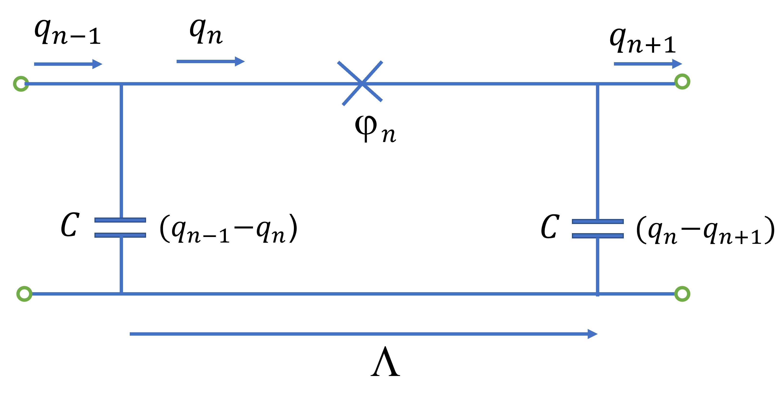
Figure 1: Discrete JTL.

In the linear approximation, Eq. (2) takes the form

$$\frac{d^{2}\varphi_{n}}{d\tau^{2}}=\varphi_{n+1}-2\varphi_{n}+\varphi_{n-1}\,.$$ (3)

The dispersion law for the eigenmodes of Eq. (3) can be easily found kittel

$$\omega(k)=2\left|\sin\left(\frac{k}{2}\right)\right|\,,\;\;k\in(-\pi,\pi]\,.$$ (4)

We will consider a modulated harmonic wave, that is a carrier wave of wave number $k_{0}$ (for the sake of definiteness we take $k_{0}>0$) and frequency $\omega_{0}=2\sin(k_{0}/2)$, modulated by a waveform $a$, which varies slowly in time and space compared to the variations of the carrier wave

$$\varphi(n,\tau)=\psi(n,\tau)+\psi^{*}(n,\tau)=a_{n}b_{n}+a_{n}^{*}b_{n}^{*}\,,$$ (5)

where

$$a_{n}=a(n,\tau)\,,\;\;\;\;b_{n}=e^{i(k_{0}n-\omega_{0}\tau)}\,,$$ (6)

III Linear approximation

Let us start from analysing Eq. (3). Because the equation is linear, we obtain decoupled equations for $\psi$ and $\psi^{*}$, and equation for $\psi$ becomes

$$\frac{d^{2}\psi_{n}}{d\tau^{2}}=\psi_{n+1}-2\psi_{n}+\psi_{n-1}\,.$$ (7)

Substituting $\psi_{n}=a_{n}b_{n}$ into (7) we obtain

$$a_{n}\frac{d^{2}b_{n}}{d\tau^{2}}+2\frac{da_{n}}{d\tau}\frac{db_{n}}{d\tau}+\frac{d^{2}a_{n}}{d\tau^{2}}b_{n}$$

$$=a_{n+1}b_{n+1}-2a_{n}b_{n}+a_{n-1}b_{n-1}\,.$$ (8)

We first focus on the r.h.s. of (III) and use the elementary formula for the discrete second derivative of the product of two functions

$$a_{n+1}b_{n+1}-2a_{n}b_{n}+a_{n-1}b_{n-1}$$

$$=a_{n}\left(b_{n+1}-2b_{n}+b_{n-1}\right)+\left(a_{n+1}-a_{n}\right)\left(b_{n+1}-b_{n}\right)$$

$$+\left(a_{n}-a_{n-1}\right)\left(b_{n}-b_{n-1}\right)+\left(a_{n+1}-2a_{n}+a_{n-1}\right)b_{n}\,.$$ (9)

Then the first term of the r.h.s. of (III) cancels against the $a_{n}d^{2}b_{n}/d\tau^{2}$-term on the l.h.s. of (III), because $b_{n}$ is by itself the solution of (3), and we arrive to the equation

$$2\frac{da_{n}}{d\tau}\frac{db_{n}}{d\tau}+\frac{d^{2}a_{n}}{d\tau^{2}}b_{n}=\left(a_{n+1}-a_{n}\right)\left(b_{n+1}-b_{n}\right)$$

$$+\left(a_{n}-a_{n-1}\right)\left(b_{n}-b_{n-1}\right)+\left(a_{n+1}-2a_{n}+a_{n-1}\right)b_{n},$$

or, more explicitly (taking into account (4)),

$$-4i\sin\left(\frac{k_{0}}{2}\right)\frac{da_{n}}{d\tau} + \frac{d^{2}a_{n}}{d\tau^{2}}=i\sin k_{0}\left(a_{n+1}-a_{n-1}\right)$$ (11)

$$+ \cos k_{0}\left(a_{n+1}-2a_{n}+a_{n-1}\right).$$

In the lowest order (with respect to the ratio of the effective modulation wave vector and $k_{0}$) approximation we should equate the first terms in the l.h.s. and r.h.s. of (11) thus obtaining

$$\frac{da_{n}}{d\tau}=-\frac{1}{2}\cos\left(\frac{k_{0}}{2}\right)\left(a_{n+1}-a_{n-1}\right)$$ (12)

and, hence,

$$\frac{d^{2}a_{n}}{d\tau^{2}}=\frac{1}{4}\cos^{2}\left(\frac{k_{0}}{2}\right)\left(a_{n+2}-2a_{n}+a_{n-2}\right)\,.$$ (13)

Substituting (13) into (11) we obtain a discrete linear Schrödinger equation (with an additional convection term that can be removed by a change of reference frame)

$$-4i\sin\left(\frac{k_{0}}{2}\right)\frac{da_{n}}{d\tau}=i\sin k_{0}\left(a_{n+1}-a_{n-1}\right)$$

$$+\cos k_{0}\left(a_{n+1}-2a_{n}+a_{n-1}\right)$$

$$-\frac{1}{4}\cos^{2}\left(\frac{k_{0}}{2}\right)\left(a_{n+2}-2a_{n}+a_{n-2}\right)\,.$$ (14)

Substituting continuous variable $x$ for the discrete variable $n$ as the argument of $a$ and expanding around $x=n$, we can present the quantities in the parentheses of (III) as

$$a_{n+1}-a_{n-1} =2\frac{\partial a}{\partial x}\,,$$ (15a)

$$a_{n+1}-2a_{n}+a_{n-1} =\frac{\partial^{2}a}{\partial x^{2}}\,,\,$$ (15b)

$$a_{n+2}-2a_{n}+a_{n-2} =4\frac{\partial^{2}a}{\partial x^{2}}\,,$$ (15c)

and after simple algebra the equation takes the form of the linear Schrödinger equation

$$i\left(\frac{\partial a}{\partial\tau}+v_{g}\frac{\partial a}{\partial x}\right)-D\frac{\partial^{2}a}{\partial x^{2}}=0\,,$$ (16)

where the group velocity $v_{g}$ and the coefficient $D$ are

$$v_{g}=\cos\left(\frac{k_{0}}{2}\right)\,,\;\;\;\;\;D=\frac{1}{4}\sin\left(\frac{k_{0}}{2}\right)\,.$$ (17)

When one looks at (16) a natural question appears: If the approximation of the underlying chain of coupled junctions by the quasi-continuum limit is extended, what will be the next-order terms in the resulting equation? We can answer this question by inspection of (15). In case of the extension mentioned above, in the derived linear Schrödinger equation there would appear additional (quasi) drift term with the third derivative with respect to $x$, and additional term with the forth derivative with respect to $x$.

IV The nonlinear Schrödinger equation

Now let us return to Eq. (2). Presenting $\varphi$ as in (5) and expanding the sine in series we get

$$\sin\varphi=\sum_{m=0}^{\infty}\frac{(-1)^{m}}{(2m+1)!}(\psi+\psi^{*})^{2m+1}\,.$$ (18)

Keeping only the first harmonics (the rotating wave approximation), we will present $\sin\varphi$ as

$$\sin\varphi = \left(\psi+\psi^{*}\right)\sum_{m=0}^{\infty}\frac{(-1)^{m}}{m!(m+1)!}|\psi|^{2m}$$ (19)

$$= \left(\psi+\psi^{*}\right)\frac{J_{1}(2|\psi|)}{|\psi|}\,,$$

where $J_{1}$ is the Bessel function. Thus we again obtain decoupled equations for $\psi$ and $\psi^{*}$, and equation for $\psi$ becomes (compare with (7))

$$\frac{d^{2}\psi_{n}}{d\tau^{2}}=\frac{J_{1}(2|\psi_{n+1}|)}{|\psi_{n+1}|}\psi_{n+1}-2\frac{J_{1}(2|\psi_{n}|)}{|\psi_{n}|}\psi_{n}$$

$$+\frac{J_{1}(2|\psi_{n-1}|)}{|\psi_{n-1}|}\psi_{n-1}\,.$$ (20)

Note that in the lowest nontrivial order (IV) takes the form

$$\frac{d^{2}\psi_{n}}{d\tau^{2}}=\left(1-\frac{|\psi_{n+1}|^{2}}{2}\right)\psi_{n+1}-2\left(1-\frac{|\psi_{n}|^{2}}{2}\right)\psi_{n}$$

$$+\left(1-\frac{|\psi_{n-1}|^{2}}{2}\right)\psi_{n-1}\,.$$ (21)

Using (5) we obtain

$$2\frac{da_{n}}{d\tau}\frac{db_{n}}{d\tau}+\frac{d^{2}a_{n}}{d\tau^{2}}b_{n}=\left(a_{n+1}-a_{n}\right)\left(b_{n+1}-b_{n}\right)$$

$$+\left(a_{n}-a_{n-1}\right)\left(b_{n}-b_{n-1}\right)+\left(a_{n+1}-2a_{n}+a_{n-1}\right)b_{n}$$

$$-d.s.d.\,,$$ (22)

where the last term in the r.h.s. of (IV) is the discrete second derivative (d.s.d.) of the product of three quantities

$$d.s.d.=a_{n+1}g_{n+1}b_{n+1}-2a_{n}g_{n}b_{n}+a_{n-1}g_{n-1}b_{n-1},$$ (23)

and

$$g_{n}\equiv g\left(|a_{n}|^{2}\right)=1-\frac{J_{1}(2|a_{n}|)}{|a_{n}|}\,.$$ (24)

The first three terms in the r.h.s. of (IV) are identical to the r.h.s. of (III). The forth term can be treated in a simpler way. In fact, the difficulty of treating the r.h.s. of (III) was connected with the fact that in the expansion with respect to the ratio of the effective modulation wave vector and $k_{0}$, the lowest order term was canceled with the appropriate term in the l.h.s. Thus we have to take into account the next order terms. There is no such cancellation for the d.s.d. term in the r.h.s. of (IV), so the term can be considered in the lowest order approximation. Among the three quantities $a_{n}$, $g_{n}$ and $b_{n}$, two ($a_{n}$ and $g_{n}$) change slowly with $n$, and the third quantity ($b_{n}$) changes fast. This is why in the r.h.s. of (23) we can ignore the difference between $a_{n}$, $a_{n-1}$ and $a_{n+1}$ (and between $g_{n}$, $g_{n-1}$ and $g_{n+1}$) and present the equation as

$$d.s.d.=a_{n}g_{n}\left(b_{n+1}-2b_{n}+b_{n-1}\right)\,.$$ (25)

Proceeding as in Section III, we obtain, instead of (16), the defocusing NLS karpman ; kosevich ; kivshar ; kevrekidis

$$i\left(\frac{\partial a}{\partial\tau}+v_{g}\frac{\partial a}{\partial x}\right)-D\frac{\partial^{2}a}{\partial x^{2}}+4Dg\left(|a|^{2}\right)a=0\,.$$ (26)

In the lowest nontrivial order with respect to $|a|^{2}$, Eq. (26) is reduced to

$$i\left(\frac{\partial a}{\partial\tau}+v_{g}\frac{\partial a}{\partial x}\right)-D\frac{\partial^{2}a}{\partial x^{2}}+2D|a|^{2}a=0\,.$$ (27)

As an additional support for the validity of Eq. (27) we will ”rederive” it in the Appendix.

V The Fermi-Pasta-Ulam-Tsingou problem

To check up our DC method, it would be appropriate to apply it to the Fermi-Pasta-Ulam-Tsingou (FPUT) problem gallavotti . The FPUT analog of (2) would be james ; james2

$$\frac{d^{2}\varphi_{n}}{d\tau^{2}}=\sin\left(\varphi_{n+1}-\varphi_{n}\right)+\sin\left(\varphi_{n-1}-\varphi_{n}\right)\,.$$ (28)

In the rotating wave approximation we again have the decoupling of the equations for $\psi$ and $\psi^{*}$. Expanding sine in Taylor series and keeping the two lowest order nonzero terms, we obtain equation for $\psi$ in the form

$$\frac{d^{2}\psi_{n}}{d\tau^{2}}=\psi_{n+1}-\psi_{n}+\psi_{n-1}-\psi_{n}$$

$$-\frac{1}{2}\left[\left|\psi_{n+1}^{2}\right|\psi_{n+1}-\psi_{n+1}^{2}\psi_{n}^{*}-2\left|\psi_{n}^{2}\right|\psi_{n}\right.$$

$$+\psi_{n}^{2}\psi_{n+1}^{*}-2\left|\psi_{n+1}^{2}\right|\psi_{n}+2\left|\psi_{n}^{2}\right|\psi_{n+1}$$

$$+\left|\psi_{n-1}^{2}\right|\psi_{n-1}-\psi_{n-1}^{2}\psi_{n}^{*}$$

$$\left.+\psi_{n}^{2}\psi_{n-1}^{*}-2\left|\psi_{n-1}^{2}\right|\psi_{n}+2\left|\psi_{n}^{2}\right|\psi_{n-1}\right]\,.$$ (29)

Following the example of Section IV we again obtain the defocusing NLS

$$i\left(\frac{\partial a}{\partial\tau}+v_{g}\frac{\partial a}{\partial x}\right)-D\frac{\partial^{2}a}{\partial x^{2}}+D^{\prime}|a|^{2}a=0\,,$$ (30)

only this time

$$D^{\prime}=\frac{1}{8b_{n}\sin\left(\frac{k_{0}}{2}\right)}\left(3b_{n+1}+3b_{n-1}-b_{n+1}^{2}b_{n}^{*}\right.$$

$$\left.-b_{n-1}^{2}b_{n}^{*}-6b_{n}+b_{n}^{2}b_{n+1}^{*}+b_{n}^{2}b_{n-1}^{*}\right)\,.$$ (31)

After simple algebra we obtain

$$D^{\prime}=2\sin^{3}\left(\frac{k_{0}}{2}\right)\,.$$ (32)

Equation (30) exactly coincides with the result of Ref. fly , in the appropriate particular case. (In that Reference, equation more general than (28) is considered.)

VI Dark solitons

The defocusing NLS equation has an interesting type of solutions, called dark solitons zakharov ; veks ; nateo ; triki . Using the opportunity, we would like to present here the derivation of these solutions, borrowed to some extent from the book kosevich (which, to the best of our knowledge, was never translated into English).

Making the transformation

$$\xi=\left(x-v_{g}\tau\right),\;\;\;\tau^{\prime}=D\tau,$$ (33)

we can present (27) as

$$i\frac{\partial a}{\partial\tau^{\prime}}-\frac{\partial^{2}a}{\partial\xi^{2}}+2|a|^{2}a=0\,.$$ (34)

Looking for the solutions of (34) in the form

$$a=Ae^{i\Phi}e^{i\Omega\tau^{\prime}},$$ (35)

where $\Omega$ is a constant, and the amplitude $A$ and the phase $\Phi$ of $a$ are some functions of $\xi$, we obtain for those functions the system of equations

$$\frac{d}{d\xi}\left(A^{2}\frac{d\Phi}{d\xi}\right) =0\,,$$ (36a)

$$\frac{d^{2}A}{d\xi^{2}}-A\left(\frac{d\Phi}{d\xi}\right)^{2}-2A^{3}+\Omega A =0\,.$$ (36b)

From (36a) we obtain

$$\frac{d\Phi}{d\xi}=\frac{c}{A^{2}}\,,$$ (37)

where $c$ is the integration constant. Substituting this expression into (36b) we obtain

$$\frac{d^{2}A}{d\xi^{2}}-\frac{c^{2}}{A^{3}}-2A^{3}+\Omega A =0\,.$$ (38)

Integrating, we obtain the differential equation of the first order

$$\left(\frac{dA}{d\xi}\right)^{2}+\frac{c^{2}}{A^{2}}-A^{4}+\Omega A^{2}=E\,,$$ (39)

where $E$ is another integration constant. We are looking for the solutions satisfying the conditions

$$\lim_{\xi\to\pm\infty}A=A_{1}.$$ (40)

Expressing the constants of integration through $\Omega$ and $A_{1}$

$$c^{2}=A_{1}^{4}\left(\Omega-2A_{1}^{2}\right)\,,\hskip 28.45274ptE=A_{1}^{2}\left(2\Omega-3A_{1}^{2}\right)\,,$$ (41)

we may present (39) as

$$\left(\frac{d\rho}{d\xi}\right)^{2}=4\left(\rho-\rho_{1}\right)^{2}\left(\rho+2\rho_{1}-\Omega\right),$$ (42)

where we have introduced $\rho=A^{2}$. Equation (42) can be easily integrated, and we obtain

$$\rho=\rho_{1}-\frac{\kappa^{2}}{\cosh^{2}\kappa\xi},$$ (43)

where $\kappa^{2}=3\rho_{1}-\Omega$. It is convenient to present Eq. $\kappa$ as

$$\kappa^{2}=A_{1}^{2}-A_{0}^{2},$$ (44)

where $A_{0}$ is the minimal value of $A$ (achieved at $\xi=0$). The function $A(\xi)$ defined by Eq. (43) is presented in Figure 2.

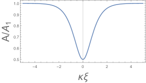
Figure 2: Dark soliton as given by Eq. (43. We have chosen $A_{0}=.5A_{1}$.

Using immobile soliton solution and the property of Galilean invariance of (34), it is easy to obtain a solution describing moving soliton. In general, if $a(\xi,\tau^{\prime})$ is a solution of (34), so is $e^{i(2V\xi+V^{2}\tau^{\prime})}a(\xi-V\tau^{\prime},\tau^{\prime})$ for arbitrary $V$.

It would be appropriate to compare the soliton given by Eq. (43) with the solitons in the JTL presented in our previous publication kogan . Those solitons were characterized by the Josephson phase, asymptotically constant at both ends of the line

$$\lim_{x\to\pm\infty}\varphi=\varphi_{1}.$$ (45)

For the solitons described by (43), the phase at both sides of the transmission line asymptotically coincides with that of a (high frequency) harmonic wave. In general, while carrier wave is all important in the present paper, there was no such wave whatsoever in our previous publication kogan .

However, it is worth to compare Figure 2 with Figure 3 borrowed from our previous publication, and showing the soliton profile calculated there. Though we didn’t use there the term dark soliton previously kogan , we see that the curves are very much similar: in both cases the amplitude goes to a constant value when $x$ ($\xi$) goes to infinities and decreases in between.

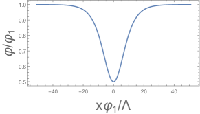
Figure 3: The soliton profile calculated in Ref. kogan . ($\Lambda$ is the period of the JTL, which in the present publication was chosen to be equal to one.)

VII Conclusions

We consider the modulated harmonic wave in the discrete series connected Josephson transmission line (JTL). We formulate the approach to the modulation problems for discrete wave equations based on discrete calculus. We check up the approach by applying it to the Fermi-Pasta-Ulam-Tsingou type problem. Applying the approach to the discrete JTL, we obtain the equation describing the modulation amplitude, which turns out to be the defocusing nonlinear Schrödinger (NLS) equation. The NLS, being the normal form for envelope waves, represents a universal model at the root of an extremely wide range of physical and other natural phenomena and applications. Furthermore, due to its rich and complex phenomenology, the NLS is also a paradigm for nonlinear spatio-temporal dynamics and is at the forefront of intense and challenging mathematical research kevrekidis . We presented a new derivation of the single soliton solution of the NLS and compared its profiles with the profile of the soliton, obtained in our previous publication.

Appendix A The approach based on Fourier integral

To additionally check up the discrete calculus approach we present here an alternative derivation of some of the results obtained in the main body of the paper, based on Fourier integral representation of the solution.

First consider the linear case. Equation (16) can be put in a more general context solitons . Let us present the solution $\psi(n,\tau)$ of a general linear equation as the Fourier integral

$$\psi(n,\tau)=\int dk\psi_{k}\exp\left\{ikn-i\omega(k)\tau\right\}\,.$$ (46)

From (46) follows

$$a(x,\tau)=\int dk\psi_{k}\exp\left\{i(k-k_{0})x-i\left[\omega(k)-\omega_{0}\right]\tau\right\}\,.$$

Differentiating with respect to $x$ we obtain

$$i\frac{\partial a}{\partial x}=-\int dk(k-k_{0})\psi_{k}$$

$$\cdot\exp\left\{i(k-k_{0})x-i\left[\omega(k)-\omega_{0}\right]\tau\right\}.$$ (48)

Differentiating with respect to $\tau$ we obtain

$$i\frac{\partial a}{\partial\tau}=\int dk\left[\omega(k)-\omega_{0}\right]\psi_{k}$$

$$\cdot\exp\left\{i(k-k_{0})x-i\left[\omega(k)-\omega_{0})\right]\tau\right\}.$$ (49)

Expanding $\omega(k)$ with respect to $k$ up to the second order we get

$$\omega(k)-\omega_{0}=\left(\frac{d\omega(k)}{dk}\right)_{0}(k-k_{0})$$

$$+\frac{1}{2}\left(\frac{d^{2}\omega(k)}{dk^{2}}\right)_{0}(k-k_{0})^{2}$$ (50)

(the derivatives are calculated at $k=k_{0}$). Comparing (A) with (A) we obtain the equation for the modulation amplitude

$$i\left[\frac{\partial a}{\partial\tau}+\left(\frac{d\omega(k)}{dk}\right)_{0}\frac{\partial a}{\partial x}\right]+\frac{1}{2}\left(\frac{d^{2}\omega(k)}{dk^{2}}\right)_{0}\frac{\partial^{2}a}{\partial x^{2}}=0\,.$$ (51)

For the dispersion law (4), Eq. (51) exactly coincides with (16).

The mnemonic rule for obtaining the equation for amplitude, modulating the harmonic wave $\exp\left\{ik_{0}n-i\omega(k_{0})\tau\right\}$, can be formulated as follows. Take the expansion of $\omega(k)$ with respect to $k$ up to the second order (A), replace $k-k_{0}$ by a spacial operator $-i\partial/\partial x$, and $\omega-\omega_{0}$ by a temporal operator $i\partial/\partial\tau$, and let (A) operate on the complex amplitude function $a$.

If we present the complex amplitude $a$ as

$$a=|a|e^{i\theta}\,,$$ (52)

the complex equation (51) can be presented as two real equations

$$\frac{\partial|a|^{2}}{\partial\tau}+\left(\frac{d\omega(k)}{dk}\right)_{0}\frac{\partial|a|^{2}}{\partial x}$$

$$+\left(\frac{d^{2}\omega(k)}{dk^{2}}\right)_{0}\frac{\partial}{\partial x}\left(|a|^{2}\frac{\partial\theta}{\partial x}\right)=0\,,$$ (53a)

$$\frac{\partial\theta}{\partial\tau}+\left(\frac{d\omega(k)}{dk}\right)_{0}\frac{\partial\theta}{\partial x}$$

$$+\frac{1}{2}\left(\frac{d^{2}\omega(k)}{dk^{2}}\right)_{0}\left[\left(\frac{\partial\theta}{\partial x}\right)^{2}-\frac{\partial^{2}|a|}{\partial x^{2}}\right]=0\,.$$ (53b)

It is interesting to compare Eq. (53) with the equations borrowed from geometric optics whitham . These equations describe a slowly varying wavetrain by equations determining the propagation of wave number and frequency

$$\frac{\partial|a|^{2}}{\partial\tau}+\frac{d\omega(k)}{dk}\frac{\partial|a|^{2}}{\partial x}+\frac{d^{2}\omega(k)}{dk^{2}}|a|^{2}\frac{\partial k}{\partial x} =0\,,$$ (54a)

$$\frac{\partial k}{\partial\tau}+\frac{d\omega(k)}{dk}\frac{\partial k}{\partial x} =0\,.$$ (54b)

It is convenient to write down Eq. (54) in a more explicit form by substituting $k=k_{0}+\partial\theta/\partial x$

$$\frac{\partial|a|^{2}}{\partial\tau} +\left(\frac{d\omega(k)}{dk}\right)_{0}\frac{\partial|a|^{2}}{\partial x}+\left(\frac{d^{2}\omega(k)}{dk^{2}}\right)_{0}\frac{\partial\theta}{\partial x}\frac{\partial|a|^{2}}{\partial x}$$

$$+\left(\frac{d^{2}\omega(k)}{dk^{2}}\right)|a|^{2}\frac{\partial^{2}\theta}{\partial x^{2}}=0\,,$$ (55a)

$$\frac{\partial^{2}\theta}{\partial x\partial\tau} +\left(\frac{d\omega(k)}{dk}\right)_{0}\frac{\partial^{2}\theta}{\partial x^{2}}+\left(\frac{d^{2}\omega(k)}{dk^{2}}\right)_{0}\frac{\partial\theta}{\partial x}\frac{\partial^{2}\theta}{\partial x^{2}}=0\,.$$ (55b)

Equation (55a) is identical to (53a). To compare (55b) with (53b), let us differentiate the latter with respect to $x$. We obtain

$$\frac{\partial\theta}{\partial x\partial\tau}+\left(\frac{d\omega(k)}{dk}\right)_{0}\frac{\partial^{2}\theta}{\partial x^{2}}+\left(\frac{d^{2}\omega(k)}{dk^{2}}\right)_{0}\frac{\partial\theta}{\partial x}\frac{\partial^{2}\theta}{\partial x^{2}}$$

$$-\frac{1}{2}\left(\frac{d^{2}\omega(k)}{dk^{2}}\right)_{0}\frac{\partial^{3}|a|}{\partial x^{3}}=0\,.$$ (56)

In the r.h.s. of Eq. (A) there is an additional term in comparison with (55b), but this term is probably negligible within the framework of the approximations made.

Now we can turn to the nonlinear case. Equation (27) can be ”rederived” following the pattern presented above. The solution of (IV) with constant amplitude $a$ is

$$\psi_{n}=ae^{i(kn-\omega t)}\,.$$ (57)

Substituting (57) into (IV) we get the nonlinear dispersion law

$$\omega(k;|a|^{2})=2\left(1-\frac{|a|^{2}}{4}\right)\left|\sin\left(\frac{k}{2}\right)\right|=\omega(k)+\omega_{2}(k)|a|^{2}\,,$$

where $\omega_{2}=-|\sin(k/2)|/2$. Hence (A) should be modified to

$$\omega-\omega_{0}=\left(\frac{d\omega(k;0)}{dk}\right)_{0}(k-k_{0})$$

$$+\frac{1}{2}\left(\frac{d^{2}\omega(k;0)}{dk^{2}}\right)_{0}(k-k_{0})^{2}+\omega_{2}(k)|a|^{2}\,.$$ (59)

If we assume that in the nonlinear case, the formula (A) is modified to a self-consistent equation

$$a(x,\tau)=\int dk\psi_{k}$$ (60)

$$\cdot \exp\left\{i(k-k_{0})x-i\left[\omega(k;|a|^{2})-\omega_{0}\right]\tau\right\}\,,$$

then (A) remains as it was in the linear case. Differentiating (60) with respect to $\tau$ we obtain

$$i\frac{\partial a}{\partial\tau} = \int dk\psi_{k}\exp\left\{i(k-k_{0})x-i\left[\omega(k;|a|^{2})-\omega_{0}\right]\tau\right\}$$ (61)

$$\cdot \left[\left(\frac{d\omega(k)}{dk}\right)_{0}(k-k_{0})+\frac{1}{2}\left(\frac{d^{2}\omega(k)}{dk^{2}}\right)_{0}(k-k_{0})^{2}\right.$$

$$+ \left.\frac{\partial\omega(k;|a|^{2})}{\partial|a|^{2}}|a|^{2}\right]\,.$$

Comparing (61) with (A) we get

$$i\left[\frac{\partial a}{\partial\tau}+\left(\frac{\partial\omega(k;a)}{\partial k}\right)_{0}\frac{\partial a}{\partial x}\right] + \frac{1}{2}\left(\frac{\partial^{2}\omega(k;a)}{\partial k^{2}}\right)_{0}\frac{\partial^{2}a}{\partial x^{2}}$$

$$-\frac{\partial\omega(k;|a|^{2})}{\partial|a|^{2}}|a|^{2} = 0\,,$$ (62)

which, for the dispersion law (A), exactly coincides with (27). We hope that the identity of the results obtained by two different approximate methods gives us additional confidence in their validity.

References

(1) E. Kogan,
Phys. Status Solidi B, 2200160 (2022).
(2) M. Remoissenet, Waves Called Solitons: Concepts and Experiments,
Third Edition,
Corrected Second Printing, Springer-Verlag Berlin Heidelberg GmbH (2003).
(3) K. O’Brien, C. Macklin, I. Siddiqi, and X. Zhang, Phys. Rev. Lett. 113, 157001 (2014).
(4) A. L. Grimsmo and A. Blais, NPJ—Quantum Inf. 3:20 (2017).
(5) A. M. Kosevich, A. S. Kovalev, Introduction into Nonlinear Physical Mechanics, Naukova Dumka, Kiev (1989).
(6)
Yu. S. Kivshar and B. Luther-Davies, Phys. Rep. 298, 81 (1998).
(7) P. G. Kevrekidis, D. J. Frantzeskakis, and R. Carretero-Gonzalez, The defocusing nonlinear Schrödinger equation: from dark solitons to vortices and vortex ring, Society for Industrial and Applied Mathematics (2015).
(8) C. Kittel, P. McEuen, and P. McEuen, Introduction to solid state physics (Vol. 8), New York: Wiley (1996).
(9) V. I. Karpman, Nonlinear Waves in Dispersive Media, Pergamon Press (1975)
(10)
V. E. Zakharov and A. B. Shabat, Sov. Phys. JETP 37, 823 (1973).
(11) D. J. Frantzeskakis, Journal of Physics A: Mathematical and Theoretical 43, 213001 (2010).
(12) A. Biswas and D. Milovic, Communications in Nonlinear Science and Numerical Simulation 15, 1473, (2010).
(13) H. Triki, T. Hayat, O. M. Aldossary, and A. Biswas, Optics & Laser Technology, 44, 2223 (2012).
(14) G. Gallavotti, ed. The Fermi-Pasta-Ulam problem: a status report, Vol. 728. Springer, 2007.
(15) G. James, J. Nonlinear Sci. 13, 273 (2003).
(16) G. James, Phys. Rev. B 70, 014301 (2004).
(17) N. Flytzanis, St. Pnevmatikos, and M. Remoissenet, J. Phys. C: Solid State Phys. 18, 4603 (1985).
(18) G. B. Whitham, Linear and Nonlinear Waves, John Wiley & Sons Inc.,
New York (1999).