Classicality, Markovianity and local detailed balance from pure state dynamics

Abstract

When describing the effective dynamics of an observable in a many-body system, the repeated randomness assumption, which states that the system returns in a short time to a maximum entropy state, is a crucial hypothesis to guarantee that the effective dynamics is classical, Markovian and obeys local detailed balance. While the latter behaviour is frequently observed in naturally occurring processes, the repeated randomness assumption is in blatant contradiction to the microscopic reversibility of the system. Here, we show that the use of the repeated randomness assumption can be justified in the description of the effective dynamics of an observable that is both slow and coarse, two properties we will define rigorously. Then, our derivation will invoke essentially only the eigenstate thermalization hypothesis and typicality arguments. While the assumption of a slow observable is subtle, as it provides only a necessary but not sufficient condition, it also offers a unifying perspective applicable to, e.g., open systems as well as collective observables of many-body systems. All our ideas are numerically verified by studying density waves in spin chains.

I Introduction

The equal-a-priori-probability postulate and the related maximum entropy principle are central axioms of statistical mechanics. For instance, for an isolated system observed to have an energy $E$ these principles imply that the correct ensemble to describe the situation is

$$\Pi_{E}/V_{E},$$ (1)

where $\Pi_{E}$ is a projector on an energy shell with energy $E$ (defined up to some small uncertainty $\Delta E$) and the normalization $V_{E}=\mbox{tr}\{\Pi_{E}\}=\exp[S_{B}(E)]$ is the exponential of the Boltzmann entropy $S_{B}(E)$. The state (1) is the familiar microcanonical ensemble, which is the central starting point of equilibrium statistical mechanics.

Moreover, the equal-a-priori-probability postulate and the maximum entropy principle continue to be useful out of equilibrium. For instance, consider two systems $A$ and $B$ in thermal contact and with average energies ${\langle{E_{A}}\rangle}$ and ${\langle{E_{B}}\rangle}$. The maximum entropy principle then implies that the correct state to describe this situation is

$$\frac{e^{-\beta_{A}H_{A}}}{Z_{A}(\beta_{A})}\otimes\frac{e^{-\beta_{B}H_{B}}}{Z_{B}(\beta_{B})}.$$ (2)

Here, the inverse temperature $\beta_{A/B}$ is chosen such that the expectation value of the Hamiltonian $H_{A/B}$ equals ${\langle{E_{A/B}}\rangle}$. Initial states such as (2), or slight generalizations of it, are predominantly used throughout the literature on nonequilibrium physics for both quantum and classical systems and independent of the employed methods (master equations, Green’s function techniques, scattering theory, etc.) de Groot and Mazur (1984); Zwanzig (2001); Nazarov and Blanter (2009); Stefanucci and van Leeuwen (2013); Schaller (2014); Strasberg (2022).

Let us continue to consider the same setup, but at a different time. Due to the thermal contact, the systems will now have energies ${\langle{E^{\prime}_{A/B}}\rangle}$ different from ${\langle{E_{A/B}}\rangle}$ in general. The maximum entropy principle then predicts again

$$\frac{e^{-\beta^{\prime}_{A}H_{A}}}{Z_{A}(\beta^{\prime}_{A})}\otimes\frac{e^{-\beta^{\prime}_{B}H_{B}}}{Z_{B}(\beta^{\prime}_{B})}$$ (3)

with suitably adapted $\beta^{\prime}_{A/B}$. But quite discomfortingly, the states (2) and (3) have different von Neumann entropies in general such that there cannot exist any Hamiltonian dynamics mapping state (2) to state (3).

A way out of this dilemma is to use the equal-a-priori-probability postulate or the maximum entropy principle only once. However, the ensuing dynamics can then quickly become very complex and intractable in practical applications. On the other hand, it is known that the repeated use of these principles gives rise to a classical stochastic process, which is Markovian and obeys local detailed balance (precise definitions of these notions and a derivation are presented below). Indeed, such a description is a common starting point of many disciplines such as stochastic thermodynamics Sekimoto (2010); Seifert (2012); Schaller (2014); Peliti and Pigolotti (2021); Strasberg (2022), which is well confirmed experimentally Bustamante et al. (2005); Ciliberto (2017).

The main focus of the present paper is to provide a justification from reversible microscopic dynamics of the repeated use of the equal-a-priori-probability postulate or the maximum entropy principle, which has been called the repeated randomness assumption by van Kampen van Kampen (2007). In fact, it seems that van Kampen has been particularly unsatisfied by it as he somewhat laconically notes at the end of his book with respect to the repeated randomness assumption that “[this] statement [has] not been proved mathematically, but it is better to say something that is true although not proved, than to prove something that is not true” (page 456 in Ref. van Kampen (2007)).

Although the high complexity of the situation does not allow us to cast our results into the form of mathematically rigorous theorems, we give plausible physical arguments together with reasonable mathematical estimates that justify the repeated randomness assumption for slow and coarse observables. Thus, based solely on one common assumption about the observable, we are able to explain the emergence of three seemingly distinct and usually separately studied concepts: classicality, Markovianity and local detailed balance. Remarkably, our derivation works for pure states and avoids any ensemble averages, by using the eigenstate thermalization hypothesis (ETH) Deutsch (1991); Srednicki (1994, 1999); Rigol et al. (2008) and typicality arguments in the form of Levy’s Lemma Popescu et al. (2006a), thereby providing a detailed microscopic understanding of why and when maximum entropy inference can be applied repeatedly.

I.1 Related literature

Our work overlaps with so many research directions that giving an exhaustive literature overview at this place appears impossible. Thus, we only list the literature that we found most influential and most closely related to our work. We ask for the forbearance of any colleagues who might think that we have missed some important publication here; it is not intentional.

First, we cannot take any credit for the idea to focus on slow and coarse observables, which is a central concept of statistical mechanics since its inception Ehrenfest and Ehrenfest (1911, 1959). In fact, the present treatment is much inspired by an old paper from van Kampen Van Kampen (1954), which well summarizes the underlying physical picture.

Second, our approach follows the philosophy of pure state statistical mechanics, which is based on the idea that quantum mechanics alone suffices to explain statistical mechanics behaviour. In fact, the use of the equal-a-priori-probability postulate and the maximum entropy principle to compute equilibrium expectation values of observables at a single time has by now been well justified within that approach Gemmer et al. (2004); D’Alessio et al. (2016); Borgonovi et al. (2016); Gogolin and Eisert (2016); Goold et al. (2016); Deutsch (2018); Mori et al. (2018).

Quite naturally, research on pure state statistical mechanics has started to focus on nonequilibrium phenomena. For instance, it has been shown that typicality arguments remain useful even out of equilibrium (“dynamical typicality” Bartsch and Gemmer (2009); Reimann (2018); Xu et al. (2022)) and can be used to derive master equations Gemmer and Michel (2006); Breuer et al. (2006); Gemmer and Breuer (2007); Hahn et al. (2020). Moreover, random matrix theory has been used to predict the time evolution of expectation values of observables Reimann (2016); Balz and Reimann (2017); Reimann and Dabelow (2019); Dabelow and Reimann (2020); Richter et al. (2020a); Dabelow and Reimann (2021) and general results on the time-scales of thermalization have been found Goldstein et al. (2013); García-Pintos et al. (2017); de Oliveira et al. (2018); Wilming et al. (2018); Nickelsen and Kastner (2019); Heveling et al. (2020); Simenel et al. (2020).

However, this research did not yet consider multi-time processes (e.g., temporal joint probabilities or correlation functions), apart from two exceptions mentioned below. Also the role of the slowness of the observable and its implications for the three properties of classicality, Markovianity and local detailed balance has not been at the focus of these previous works. Instead, these properties have been typically investigated within a (repeated) ensemble average approach to statistical mechanics.

First, we comment on the emergence of classicality, which is commonly explained with decoherence Zurek (2003); Joos et al. (2003); Schlosshauer (2019). It combines two ideas: first, all systems are essentially open systems and, second, open systems decohere, i.e., their density matrix becomes diagonal in a particular fixed basis (“pointer basis”). We emphasize that it is not our intention to question the correctness of the decoherence approach. While there is fundamental criticism (see, e.g., Refs. Leggett (2002); Ballentine (2008); Knipschild and Gemmer (2019); Berjon et al. (2021)), our results are not in contradiction with decoherence, which is motivated by the central question: “Which is the preferred measurement basis?” Zurek (1981) Instead, we consider a different perspective and significantly extend the realm in which quantum dynamics appears classical. In particular, from the perspective of pure state statistical mechanics one would like to derive classical behaviour for a single wave function $|\psi\rangle$ and realistic many-body systems. Yet, for any observable that does not have a definite deterministic outcome when measured in state $|\psi\rangle$, $|\psi\rangle$ must necessarily have coherences in the eigenbasis of that observable. Global decoherence can therefore not happen, as a mathematical fact of linear algebra, but still one would expect that also pure states can behave classical in an appropriate sense. Here, by extending previous numerical studies Gemmer and Steinigeweg (2014); Schmidtke and Gemmer (2016), we argue that slow and coarse observables behave classical and estimate deviations from classical behaviour to be exponentially small in the system size. Our approach hints at a possibly deep connection between pure state statistical mechanics, the ETH and classical behaviour, which remains unrecognized within the conventional open quantum systems paradigm, where the bath is typically modeled as integrable and as staying approximately in a canonical ensemble Breuer and Petruccione (2002); de Vega and Alonso (2017). Our approach also provides physical substance to recent abstract studies of multi-time classicality Smirne et al. (2018); Strasberg and Díaz (2019); Milz et al. (2020a, b) and it might offer interesting insights for the consistent histories approach to quantum mechanics Griffiths (1984); Omnès (1992); Griffiths (2019) and quantum Darwinism Zurek (2009, 2022), as recently explored by one of us Strasberg (2023).

Secondly, much recent research has been devoted to understanding non-Markovianity in quantum systems Rivas et al. (2014); Breuer et al. (2016); Li et al. (2018); Milz and Modi (2021). This research mostly revolved around the question how to properly define and quantify non-Markovianity, but surprisingly little rigorous and general results are known about the question which physical properties give rise to Markovianity. For instance, it is known that open quantum systems are Markovian in the weak coupling limit Dümcke (1983), which literally requires to scale the system-bath coupling to zero, among other questionable assumptions. Indeed, without that limiting procedure it has been claimed that no physical system is Markovian Ford and O’Connell (1996). Somewhat reconciling these two results, recent research has highlighted that typical processes are almost Markovian Figueroa-Romero et al. (2019, 2021), but with the caveat that “typical” is defined with respect to an abstract mathematical measure, which is likely not typical in reality. Moreover, we would like to point out that an important aspect of (non-)Markovianity cannot be captured when using ensemble averages instead of pure states. Indeed, if the system dynamics is non-Markovian, this implies that the system reacts very sensitively to different microstates of the bath, or, conversely, if the system dynamics is insensitive to the precise state of the bath, it must be Markovian. But by using an initial ensemble average over a highly mixed canonical ensemble, the influence from the different microstates is washed out. To the best of our knowledge, only recently the question of (non-)Markovianity has been studied for pure states Figueroa-Romero et al. (2019, 2021). We believe, however, that the result that almost all open quantum systems are almost Markovian is too strong. Based on our findings it seems that Markovianity is also crucially related to the observable we are probing, and cannot be deduced from the unitary dynamics alone as in Refs. Figueroa-Romero et al. (2019, 2021).

Thirdly, the property of local detailed balance ensures thermodynamic consistency at each time step of the process and it is thus build into the framework of stochastic thermodynamics Sekimoto (2010); Seifert (2012); Schaller (2014); Peliti and Pigolotti (2021); Strasberg (2022). For systems that equilibrate in the macroscopic sense, it has been derived in its most general form by van Kampen based on the repeated randomness assumption Van Kampen (1954). Since the notion of local detailed balance, which is sometimes also called “detailed balance” (without the attribute “local”) or “microreversibility”, might be less familiar to some readers, we explain it more thoroughly later on.

We end this short literature survey with two remarks for specialists in open quantum systems theory. First, the repeated randomness assumption is commonly known as the Born approximation in this field. Second, our work is motivated by a lack of any satisfactory explanation of the repeated randomness assumption, but sceptical voices might claim that Nakajima-Zwanzig projection operator techniques show that the Born approximation is only needed once in the derivation of the (quantum) master equation Breuer and Petruccione (2002). There are, however, two subtle pitfalls. First, this statement is only true for the exact Nakajima-Zwanzig master equation: once one applies perturbation theory the failure of the Born approximation at later times can give rise to additional correction terms even to lowest order in the perturbation theory Mitchison and Plenio (2018). Second, we are here interested in processes characterized by multi-time statistics in contrast to the single-time statistics that are accessible with a master equation. Related recent work has also investigated the multi-time statistics for pure state dynamics using long-time averages Dowling et al. (2023a, b), which we do not use here. From the perspective of open quantum system theory, our results thus explain why and when the intuitive Born approximation is justified even though the exact unitarily time-evolved system-bath state no longer complies with the Born approximation (for a related numerical study see Ref. Kolovsky (2020)). Equivalently, if one insists to apply the Born approximation only at the initial time, our results microscopically justify the quantum regression theorem Li et al. (2018).

I.2 Outline

Section II starts by introducing an intuitive picture for our setup while establishing notation along the way (Sec. II.1), gives a first explanation of “slow” observables (Sec. II.2), and briefly reviews the main tools we are using, namely the ETH and Levy’s Lemma (Sec. II.3).

Sections III, IV and V contain the core results of this paper about classicality, Markovianity and local detailed balance, respectively. They start with a brief definition and discussion of the respective notion together with their derivation based on the repeated randomness assumption. Afterwards, we show how each of these properties arises from pure state dynamics.

Section VI then presents numerical results for density waves in a spin chain, which confirm our main ideas. Since we have tested many features numerically, we decided to shift some of them to a supplemental material to keep the main manuscript focused.

However, the numerical results also raise awareness about various subtleties, some of which are discussed more generally in Sec. VII. In particular, we return to the subtle notion of “slowness” and questions related to multiple observables (Sec. VII.1). Moreover, Sec. VII.2 discusses which properties of the process are not fixed by our general considerations (namely the time scales).

Finally, Sec. VIII presents conclusions. Furthermore, two short technical proofs are relegated to the Appendix.

II Preliminaries

II.1 Setup and intuitive picture

We consider a time-independent isolated quantum system with Hamiltonian $H=\sum_{k}E_{k}|k{\rangle\langle}k|$ with ordered eigenenergies $E_{k+1}\geq E_{k}$ and eigenvectors $|k\rangle$. Owing to the time-independence, we can and will restrict ourselves to some microcanonical energy shell, which is small on a macroscopic scale but large on a microscopic scale, i.e., the dimension $D$ of the corresponding microcanonical Hilbert space ${\cal{H}}$ obeys $D={\cal{O}}(10^{N})$ with $N$ the number of particles in the system. For simplicity we assume energy to be the only conserved quantity, other conserved quantities (such as particle number) could be readily included in the description. Moreover, we set $\hbar\equiv 1$ such that the time evolution of a pure state is given by $|\psi(t)\rangle=\sum_{k}e^{-iE_{k}t}c_{k}|k\rangle$ with $c_{k}\in\mathbb{C}$ satisfying $\sum_{k}|c_{k}|^{2}=1$.

We are interested in the evolution of an observable $X=\sum_{x=1}^{M}\lambda_{x}\Pi_{x}$ with eigenvalues $\lambda_{x}$ and corresponding eigenprojectors $\Pi_{x}$, which divide the Hilbert space ${\cal{H}}=\bigoplus_{x}{\cal{H}}_{x}$ into subspaces ${\cal{H}}_{x}$. Moreover, we are only interested in coarse observables, which means that the number $M$ of different projectors (or potential measurement results) is much smaller than $D$. This assumption will be satisfied for any realistic experiment with a many-body system. Equivalently, a coarse observable is characterized by subspaces ${\cal{H}}_{x}$ whose dimension is typically very large: $V_{x}\equiv\dim{\cal{H}}_{x}\gg 1$. We will refer to $V_{x}$ as a volume in view of Boltzmann’s entropy concept $S_{B}(x)\equiv\ln V_{x}$ ($k_{B}\equiv 1$ throughout), which plays an important role later on. We further call each $x$ a macrostate, despite the fact that it does not need to be macroscopically large in an intuitive sense. For instance, $x$ could label an energy eigenvalue of an open quantum system, which is still a coarse observable in the full system-bath space.

We write $\Pi_{x}=\sum_{\alpha}|x_{\alpha}{\rangle\langle}x_{\alpha}|$, where $\alpha$ sums over the microstates $|x_{\alpha}\rangle$ spanning ${\cal{H}}_{x}$. Decomposing the wave function in the eigenbasis of $X$ gives $|\psi(t)\rangle=\sum_{x,\alpha}c_{x,\alpha}(t)|x_{\alpha}\rangle$ with $c_{x,\alpha}(t)=\sum_{k}e^{-iE_{k}t}c_{k}{\langle{x_{\alpha}|k}\rangle}$. The normalization condition $\sum_{x,\alpha}|c_{x,\alpha}(t)|^{2}=1$ defines a sphere $\mathbb{S}^{2D-1}\subset\mathbb{C}^{D}\cong\mathbb{R}^{2D}$ of dimension $2D-1$ and radius 1, where the factor 2 arises because $c_{x,\alpha}(t)$ has a real and imaginary part. Since a generic many-body system is non-integrable, the eigenenergies $E_{k}$ are incommensurate (apart from accidential degenercies) and the phases $e^{-iE_{k}t}$ vary erratically with $k$. Moreover, a typical wave function, in particular one prepared out of equilibrium, has many non-vanishing coefficients $c_{k}$ Reimann (2008); Linden et al. (2009); Wilming et al. (2019). This implies that the $c_{x,\alpha}(t)$ vary in a practically unpredictable way. Thus, we like to picture the evolution of $|\psi(t)\rangle$ in the eigenbasis of $X$ as a random walk on the high dimensional sphere $\mathbb{S}^{2D-1}$ as illustrated in Fig. 1.

Strictly speaking, this picture is incorrect. The evolution is not truely random and, since the coefficients $c_{k}$ are constant and only the phases $e^{-iE_{k}t}$ vary in time, the state can only explore a $D$ dimensional submanifold (a hypertorus) on the sphere $\mathbb{S}^{2D-1}$. Unfortunately, our restriction of living in a three-dimensional world does not allow us to sketch this properly. However, what is important (and correct) for our purposes is that the state explores a high dimensional space in a sufficiently unbiased and random fashion.

On the sphere $\mathbb{S}^{2D-1}$, we can picture ${\cal{H}}_{x}$ as lower dimensional subspaces $\mathbb{S}^{2V_{x}-1}$ defined by all states $|\psi_{x}\rangle=\sum_{\alpha}c_{x,\alpha}|x_{\alpha}\rangle$ satisfying $\sum_{\alpha}|c_{x,\alpha}|^{2}=1$. These spaces are of measure zero (with respect to $\mathbb{S}^{2D-1}$) and therefore indicated as lines on the two-dimensional surface of the sphere in Fig. 1. A state drawn at random will typically overlap with many such volumes (which is again hard to sketch), i.e., it has coherences between different macrostates. However, many thermodynamic variables are characterized by having one dominant subspace $x$ with $V_{\text{eq}}\equiv V_{x}\gg V_{y}$ for all $y\neq x$, which can be identified with the equilibrium subspace (in Fig. 1 the equator, having the longest line, corresponds to the subspace with the largest volume) Goldstein et al. (2010). Most randomly drawn states will lie very close to this equilibrium subspace.

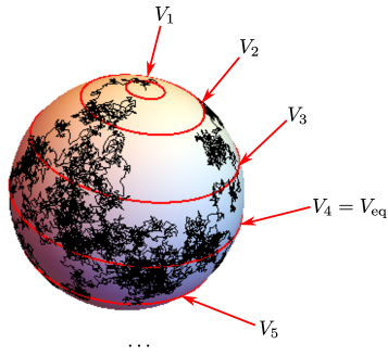
Figure 1: Sketch of $\mathbb{S}^{2D-1}$ with subspaces ${\cal{H}}_{x}$ labeled with their volumes $V_{1},V_{2},\dots$ (red lines). The state (here initialized at the north pole) performs an effective random walk on the surface of the sphere and, eventually, spends most time close to the equilibrium subspace, which has the largest volume (here $V_{4}=V_{\text{eq}}$).

The present analogy suggests that the evolution of a state vector of a non-integrable system can be approximately viewed as a diffusion process on a high dimensional subspace of $\mathbb{S}^{2D-1}$. If we have taken into account all conserved quantities and if $X$ is the only relevant slowly varying observable (more on this in Sec. VII.1), then this diffusion process should be isotropic, where the trajectory of the state vector does not preferably select certain ‘narrow’ regions of $\mathbb{S}^{2D-1}$ during its evolution. Based on this intuition, it appears plausible that the evolution of the probabilities $p_{x}(t)={\langle{\psi(t)|X|\psi(t)}\rangle}$ should be describable by a classical Markov process. It is classical because it is unlikely that the enormous number of tiny amplitudes $c_{x,\alpha}(t)$ interfere constructively and thus give rise to a large detectable coherent effect, as we explain in greater detail in Sec. III. It is Markovian because two slightly different initial microstates behave approximately the same from a coarse-grained point of view. Moreover, the isotropic diffusion causes an initial nonequilibrium state, i.e., a state confined to a low entropy region of small volume, to evolve towards larger volume regions in such a way that entropy continuously increases, which is the condition of local detailed balance.

The goal of this paper is to make this intuition as rigorous as possible by combining tools from the ETH and typicality with plausible physical assumptions.

II.2 Slow observables

Slowness is a crucial ingredient not only in our derivation but in many approaches to statistical mechanics, yet defining it precisely is not simple. Roughly speaking, we call an observable slow if its expectation value ${\langle{X}\rangle}(\tau)$ evolves on a characteristic time scale

$$\frac{1}{\delta e}\gg\tau\gg\frac{1}{\Delta E}$$ (4)

for initial nonequilibrium states. Here, $\Delta E$ is the width of the microcanonical energy window such that $1/\Delta E$ corresponds to the time the system needs to evolve between two orthogonal microstates, which follows rigorously from the quantum speed limit Mandelstam and Tamm (1945); Deffner and Campbell (2017). It is typically an extremely short time scale, impossible to resolve in most mesoscopic or macroscopic experiments since $\Delta E\sim\sqrt{N}$. On the other end of the spectrum, $1/\delta e$ with $\delta e\approx\Delta E/D\sim 10^{-N}$ the mean level spacing is an extremely long time scale known as the Heisenberg time. It corresponds to the time needed for a quantum system to explore the full available Hilbert space. Thus, a slow observable evolves slow compared to the microscopic motion of the system, but fast enough to be recognizable in an experiment as a nonequilibrium dynamics.

Thinking further about it, we see that we can mathematically characterize a slow observable $X$ as being a narrowly banded matrix in an ordered energy eigenbasis. To see this, note that

$${\langle{X}\rangle}(\tau)=\sum_{k,\ell}e^{i\omega_{k\ell}\tau}c_{k}^{*}c_{\ell}X_{k\ell}$$ (5)

with the transition frequency $\omega_{k\ell}=E_{k}-E_{\ell}$ and the matrix elements $X_{k\ell}={\langle{k|X|\ell}\rangle}$. If we want to ensure that this expression varies on the time scale specified in Eq. (4) for all nonequilibrium initial states (within a microcanonical energy window), we need to demand that $X_{k\ell}$ differs significantly from zero only for frequencies $\omega_{kl}\in[-\delta E,\delta E]$ with the width $\delta E$ satisfying $\delta e\ll\delta E\ll\Delta E$, i.e., $X$ is narrowly banded.

Another perspective on slowness is offered by Heisenberg’s equation of motion by defining the evolution time-scale of $X$ as $\tau\equiv\|X\|/|d{\langle{X}\rangle}/dt|$ with the operator norm $\|\cdot\|$. Then, Heisenberg’s equation implies

$$\tau=\frac{\|X\|}{|{\langle{[H,X]}\rangle}|}\geq\frac{\|X\|}{\|[H,X]\|},$$ (6)

where we used $|\mbox{tr}\{A\rho\}|\leq\|A\|$ for any density matrix $\rho$. Now, if we demand

$$\|[H,X]\|\ll\|H\|\|X\|,$$ (7)

one finds $\tau\gg 1/\|H\|$, which reduces to the right inequality in Eq. (4) if we define the (arbitrary) energy of the microcanonical energy shell to be zero. In fact, we show in Appendix A that a narrowly banded matrix implies Eq. (7). Unfortunately, we were not able to show that Eq. (7) implies a narrowly banded $X$, albeit we also found no counterexample. It seems likely to us that counterexamples require precisely tuned observables and states. For most practical purposes it thus seems reasonable to assume that the condition of Eq. (7) is equivalent to a narrowly banded $X$.

Apart from the abstract mathematical property of slowness, finding precise yet generic physical conditions for the existence of slow observables $X$ is not trivial. However, there are a few important cornerstones known that we list here. First, an obvious class is given by problems that can be cast into the form

$$H=H_{0}+\epsilon V,\leavevmode\nobreak\ \leavevmode\nobreak\ \leavevmode\nobreak\ [H_{0},X]=0,\leavevmode\nobreak\ \leavevmode\nobreak\ \leavevmode\nobreak\ [V,X]\neq 0,$$ (8)

and where $\epsilon\ll 1$ is a small perturbative parameter. In fact, this class of problems is omnipresent in the literature. For instance, for weakly coupled open quantum systems one has $H_{0}=H_{S}+H_{B}$ with $H_{S}$ ($H_{B}$) the system (bath) Hamiltonian and $V$ their interaction. Then, we see that the energy of a weakly coupled open quantum system $X=H_{S}$ is a slow observable.

More generally, it can be shown that local observables of local Hamiltonians are described by banded matrices in the energy eigenbasis Beugeling et al. (2015); Arad et al. (2016); de Oliveira et al. (2018). In particular, Refs. Arad et al. (2016); de Oliveira et al. (2018) have shown a bound of the form

$$|X_{k\ell}|\leq\|X\|\exp\big{(}-a[|\omega_{k\ell}|-b\ln(c|\omega_{k\ell}|)]\big{)}$$ (9)

for suitable constants $a$, $b$ and $c$ describing local properties of $H$ and $X$. While it is possible that these constants behave unfavourably in a particular application (resulting in a matrix that is not narrowly banded), they are importantly independent of the system size.

Similarly, also the ETH conjectures that thermodynamically relevant observables are banded matrices characterized by a smooth envelope function $F(\omega_{k\ell})$ that decays for large $\omega_{k\ell}$ (see below). However, generic results about the decay of this function are not known to the best of our knowledge.

Finally, another class of slow observables is given by extensive sums of local observables, which we like to illustrate with an example. Consider the 1D Ising model $H=\sum_{i=1}^{L}\sigma_{z}^{i}+\sum_{i=1}^{L}\sigma_{x}^{i}\sigma_{x}^{i+1}$ of length $L$ with periodic boundary conditions and $\sigma_{x,y,z}^{i}$ the standard Pauli matrices of spin $i$ (we ignore any prefactors because they do not change our point). Moreover, let the observable be the total magnetization $X=\sum_{i=1}^{L}\sigma_{z}^{i}$. Then, one finds that all operator norms in Eq. (7) scale with $L$ and Eq. (7) reduces to $L\ll L^{2}$, which is clearly satisfied for large $L$. This example illustrates the important point that observables can be slow although it is not possible to identify a perturbative parameter $\epsilon$ in the Hamiltonian, as it was possible for the class of observables characterized by Eq. (8).

While we have focused here on presenting generic properties of slowness, they do not guarantee an isotropic or unbiased diffusion in Hilbert space as described in our intuitive picture in Sec. II.1. Understanding this is much more subtle and closely related to the complicated problem of ergodicity. In our case, ergodicity (exploration of the full microcanonical energy shell during the dynamics) cannot happen for reasons explained in Sec. II.1. However, what matters is a sufficiently smooth observable such that even comparably short evolution times give representative (“typical”) averages Khinchin (1949). It is a known and hard problem to identify these observables rigorously, but we return to this question it greater detail in Sec. VII.1 in context of multiple slow observables after having developed an understanding for a single observable.

II.3 ETH and Levy’s Lemma

In our derivation we make use of two tools, which have become widely used by now. First, the ETH conjectures that matrix elements in the energy eigenbasis of thermodynamically relevant observables $X$ can be written as

$$X_{k\ell}=\delta_{k\ell}{\langle{X}\rangle}_{\text{mic}}+\frac{1}{\sqrt{D}}F(\omega_{k\ell})R_{k\ell}.$$ (10)

Here, ${\langle{X}\rangle}_{\text{mic}}$ is the expectation value of $X$ with respect to the microcanonical ensemble (1), $F(\omega)$ is a smooth function of order one for observables with a second central moment (or variance in the microcanonical ensemble) of order one, $\mbox{tr}\{X^{2}\}/D-\mbox{tr}\{X\}^{2}/D^{2}={\cal{O}}(1)$, and $R_{k\ell}$ are pseudorandom numbers of zero mean and unit variance. How “random” the $R_{k\ell}$ behave is under current investigation Foini and Kurchan (2019); Chan et al. (2019); Murthy and Srednicki (2019); Richter et al. (2020b); Brenes et al. (2021); Wang et al. (2022); Dymarsky (2022). Finally, note that the ETH is a hypothesis, but it is considered to hold for a wide class of many-body systems in nature, see Refs. D’Alessio et al. (2016); Deutsch (2018); Mori et al. (2018) and references therein for more information.

Our second tool is Levy’s Lemma. To state it precisely, let $f:\mathbb{S}^{2D-1}\rightarrow\mathbb{R}$ be any function defined on the hypersphere of dimension $2D-1$. Moreover, let $\eta$ be the Lipschitz constant of $f$ with respect to the Euclidean space $\mathbb{R}^{2D}$, which is the natural embedding of $\mathbb{S}^{2D-1}$. If $f$ is differentiable, then $\eta=\sup|\nabla f|$. Moreover, let ${\langle{f}\rangle}=\mu[f(\psi)]$ denote the Haar random average of $f$ over the hypersphere $\mathbb{S}^{2D-1}$. Note that the Haar measure is the only measure invariant under all unitary transformations and therefore the natural unbiased measure on the sphere. Then, Levy’s Lemma says that

$$\mu\big{[}|f-{\langle{f}\rangle}|>\epsilon\big{]}\leq 4\exp\left(-\frac{\epsilon^{2}2D}{9\pi^{3}\eta^{2}}\right).$$ (11)

One easily notices that even for small $\epsilon$ the right hand side quickly tends to zero for a sufficiently large dimension $D$. Thus, colloquially speaking, Levy’s Lemma says that every “nice” function $f(\psi)$ on a high dimensional hypersphere is essentially constant, i.e., it varies very little with varying $\psi$. Levy’s Lemma gives typicality arguments a firm mathematical basis and it has been used to show that thermal equilibrium states are ubiquituous with respect to the Haar measure Popescu et al. (2006a), among other applications Linden et al. (2009); Figueroa-Romero et al. (2019, 2021); Reimann (2015). In general, it is a consequence of a phenomenon known as measure concentration Talagrand (1996); Milman and Schechtman (2001).

III Classicality

How to explain the emergence of classical behaviour from an underlying quantum description is an important foundational and, nowadays, also a practical very relevant question. Clearly, the quantum-to-classical boundary is not one-dimensional and there are many ways to define it. For instance, one might use Bell inequalities to find out whether a bipartite quantum state has correlations, which cannot be explained classically. This certainly legitimate characterization, however, only probes static quantum features of a state. Here, instead, we are interested in a process and the question whether the dynamics of $X$ reveals quantum features. Our characterization is therefore based on the following question (see also Refs. Gemmer and Steinigeweg (2014); Schmidtke and Gemmer (2016); Smirne et al. (2018); Strasberg and Díaz (2019); Milz et al. (2020a, b); Strasberg (2023)): Can an experimenter distinguish the measurement statistics of $X$ from a classical stochastic process?

To define this rigorously, we denote the probability to obtain outcomes $x_{n},\dots,x_{1}$ at times $t_{n}>\dots>t_{1}$ as

$$\begin{split}p&(x_{n},\dots,x_{1})=\\ &\mbox{tr}\{\Pi_{x_{n}}U_{n}\dots U_{2}\Pi_{x_{1}}U_{1}\rho(t_{0})U_{1}^{\dagger}\Pi_{x_{1}}U_{2}^{\dagger}\dots U_{n}^{\dagger}\},\end{split}$$ (12)

where $\rho(t_{0})$ is some initial state and $U_{k}=e^{-iH(t_{k}-t_{k-1})}$ the unitary time evolution operator from $t_{k-1}$ to $t_{k}$. Note that the probabilities (12) can be experimentally reconstructed by repeated projective measurements of the (otherwise) isolated quantum system and statistical sampling. Next, suppose that the experimenter decides not to measure the system at some time $t_{\ell}$ with $\ell<n$. We denote the probability to obtain apart from $x_{\ell}$ the same outcomes $x_{n},\dots,x_{\ell+1},x_{\ell-1},\dots,x_{1}$ by $p(x_{n},\dots,\cancel{x_{\ell}},\dots,x_{1})$, which is obtained from Eq. (12) by dropping the two projectors $\Pi_{x_{\ell}}$. Now, the defining property of a classical stochastic process is Kolmogorov (2018)

$$\sum_{x_{\ell}}p(x_{n},\dots,x_{\ell},\dots,x_{1})=p(x_{n},\dots,\cancel{x_{\ell}},\dots,x_{1}),$$ (13)

which is also known as the Kolmogorov consistency condition or “probability sum rule”. In words, a classical stochastic process is characterized by the property that not measuring is equivalent to averaging over the respective measurement outcomes. Clearly, for a quantum process Eq. (13) is in general not satisfied because quantum measurements are disturbing and the classical example of the double slit experiment in Fig. 2 is used to illustrate the breaking of the Kolmogorov consistency condition in the quantum world.

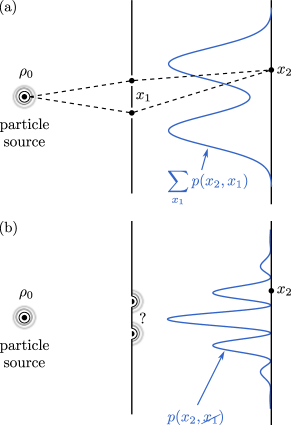
Figure 2: A coherent source of particles $\rho_{0}$ is sent to a detection screen through a double slit. (a) The particle’s location at the double slit ($x_{1}$) and at the detection screen ($x_{2}$) is measured, allowing to speak about a definite trajectory (indicated by dashed lines) but causing a loss of wave properties. (b) Only the position at the detection screen is measured, resulting in an interference pattern. Clearly, Eq. (13) is broken.

We emphasize again that Eq. (13) is not the only way to characterize classicality, but it has a number of desirable features. Among them are, for instance, that the Kolmogorov consistency condition implies the validity of all Leggett-Garg inequalities Emary et al. (2014). It is also implied by the “consistency condition” imposed in the histories interpretation of quantum mechanics Griffiths (1984); Omnès (1992); Griffiths (2019) and it guarantees that we can apply classical reasoning to understand the physics even in absence of measurements. Importantly, however, testing the validity of Eq. (13) requires only the ability to measure $X$ and is independent of the interpretation of quantum mechanics. Finally, note that a quantum system can behave classical with respect to one observable $X$, but not with respect to another observable $Y$. An extended discussion, in particular in relation to other approaches, is provided in Ref. Strasberg (2023).

We proceed by confirming that the repeated randomness assumption implies classical measurement statistics. To this end note that all that the experimenter knows about the state at time $t_{\ell}$ is some probability distribution $p(x_{\ell}|x_{\ell-1},\dots,x_{1})$ conditioned on earlier results $x_{\ell-1},\dots,x_{1}$. The state which maximizes the entropy given that information is

$$\rho_{\text{max ent}}(t_{\ell})\equiv\sum_{x_{\ell}}p(x_{\ell}|x_{\ell-1},\dots,x_{1})\frac{\Pi_{x_{\ell}}}{V_{x_{\ell}}}.$$ (14)

Note that we would have obtained the same state by applying the equal-a-priori-probability postulate, which associates to every subspace $x$ the state $\Pi_{x}/V_{x}$ independent of the probability distribution. For our setup the maximum entropy principle and the equal-a-piori-probability postulate thus turn out to be the same. In general, this is not the case, although both principles still express the same basic idea: maximize ignorance given the experimentally available information.

Next, notice that the state (14) is block diagonal with respect to the $\Pi_{x}$ basis. This implies in particular that

$$\sum_{x}\Pi_{x}\rho_{\text{max ent}}(t_{\ell})\Pi_{x}=\rho_{\text{max ent}}(t_{\ell}),$$ (15)

where the operation on the left hand side is a “dephasing” operation (with respect to $X$). One easily confirms that the validity of Eq. (15) implies the validity of Eq. (13).

It might be tempting to explain the block diagonal form of the state (14) by using decoherence. However, we are dealing with an isolated and not an open system here. Assuming the validity of a block diagonal state for all times either implies that the probabilities $p(x_{t})=\mbox{tr}\{\Pi_{x}\rho(t)\}$ do not change in time (i.e., $X$ is a conserved quantity) or that the von Neumann entropy of the state is not conserved. To illustrate this, consider an initially pure state $\rho(t_{0})=|\psi_{0}{\rangle\langle}\psi_{0}|$. If there are non-trivial dynamics with some probability flux, say, from $x$ to $y$, then this implies that $\Pi_{x}\rho(t)\Pi_{y}\neq 0$ for $x\neq y$ for at least some times $t$, i.e., the state cannot be block diagonal. The main contribution of this section is to give a generic explanation for the emergence of classical measurement statistics obeying Eq. (13) despite the presence of a lot of coherences.

In the following, we consider three arbitrary times $t_{2}>t_{1}>t_{0}$ and a nonequilibrium initial state $\rho(t_{0})$. The probability to measure $x_{2}$ and $x_{1}$ is

$$p(x_{2},x_{1})=\mbox{tr}\{\Pi_{x_{2}}U_{2}\Pi_{x_{1}}U_{1}\rho(t_{0})U_{1}^{\dagger}\Pi_{x_{1}}U_{2}^{\dagger}\}$$ (16)

and the probability to only measure $x_{2}$ is $p(x_{2},\cancel{x_{1}})=\mbox{tr}\{\Pi_{x_{2}}U_{2}U_{1}\rho(t_{0})U_{1}^{\dagger}U_{2}^{\dagger}\}$. If the process is classical, the quantum contribution

$$Q\equiv p(x_{2},\cancel{x_{1}})-\sum_{x_{1}}p(x_{2},x_{1})\leavevmode\nobreak\ \in[-1,+1]$$ (17)

should be zero. Below, we estimate that $Q\sim D^{-\alpha}$ with $\alpha>0$, i.e., $Q$ is exponentially small in the particle number and thus essentially zero for all reasonable experiments involving many-body systems. Note, however, that the precise value of the exponent $\alpha$ depends on the situation and is not universal.

We emphasize that smallness of $Q$ in Eq. (17) does not imply a similarly small deviation from equality in Eq. (13) in full generality, rather the extension to an arbitrary number $n$ of time steps requires a separate, technically demanding argument. We recall that also the decoherence approach shows only decoherence of the open system density matrix, which is not sufficient to compute $n$-time correlation functions without additional assumptions.

The following derivation is the technically most involved part of the present paper. This comes from the fact that we try to derive a statement valid for all slow and coarse observables satisfying the ETH, even out of equilibrium. Since the ETH is assumed to hold for a wide class of realistic many-body systems in nature, our statement is widely applicable. However, recalling that nonequilibrium many-body dynamics result from a complex interplay between the initial state, the observable and the Hamiltonian (or time-evolution operator), and recalling that there is no systematic way (e.g., in form of a perturbation theory) to take their intricate correlations into account, it becomes evident that we must restrict our derivation to estimates and approximations. Although there is no justification from first principles known for them, we believe them to be plausible.

Therefore, the derivation below cannot be claimed to have the status of a rigorous mathematical theorem. Counterexamples do exist, and we also partially address them in this article. Nevertheless, the derivation below adds considerable evidence that counterexamples are not generic. Given that, to the best of our knowledge, a microscopic derivation of the Kolmogorov consistency condition has never been presented for an isolated system, we find the wide scope of the derivation below certainly remarkable and, at the end, also intuitively correct: since human senses are coarse in space and time, this explains the emergence of a classical world for many observables even though the true quantum state might not be diagonal (decohered) in all the eigenbases of these observables.

III.1 Microscopic derivation

How can it be that a state containing a lot of coherences gives rise to classical measurement statistics? Roughly speaking, the idea is that the contribution of the coherences to the probabilities appearing in Eq. (13) is given by a sum of many very small and randomly oscillating terms such that the chance that all coherences for a coarse observable of a non-integrable many-body system align up in phase becomes very small. Thus, the derivation below is essentially of statistical nature, similar to the derivation of the second law. From that perspective it is not suprising that we have to content ourselves with some rough but reasonable estimates in general (more specific models might allow, of course, for more specific conclusions, see also Ref. Strasberg (2023)). Similar to the second law, for each observable $X$ one can find precisely tuned states and times for which classicality is violated, yet these situations are non-generic.

Step 1: Experimentally realistic initial state dependence

We begin with considerations about the initial state $\rho(t_{0})$. In general, the further away the state is from equilibrium the stronger it is correlated with the matrix elements of $X$. On the other hand, since $X$ is a coarse observable, knowing the probabilities $p(x_{0})=\mbox{tr}\{\Pi_{x_{0}}\rho(t_{0})\}$ does not completely determine $\rho(t_{0})$, but still leaves room for some freedom. Finding the right balance between this freedom and the required correlations is what makes the problem delicate. Here, we solve this problem by thinking experimentally and by explicitly modelling the state preparation procedure. To this end, let $\psi_{0}=|\psi_{0}{\rangle\langle}\psi_{0}|$ be a pure state before the preparation. Then, any state preparation can be modeled by an instrument $\{{\cal{A}}_{r}\}$ Kraus (1983); Breuer and Petruccione (2002); Milz and Modi (2021); Strasberg (2022). Here, each ${\cal{A}}_{r}$ is a completely positive map labeled by some (abstract) measurement outcome $r$ and ${\cal{A}}\equiv\sum_{r}{\cal{A}}_{r}$ is a completely positive and trace preserving map. This means that the state preparation given outcome $r$ can be written as

$$\psi_{0}\mapsto\rho(t_{0})={\cal{A}}_{r}\psi_{0}=\sum_{\alpha=1}^{g}K_{\alpha}(r)\psi_{0}K_{\alpha}^{\dagger}(r)$$ (18)

with operators $K_{\alpha}(r)$ satisfying $\sum_{\alpha=1}^{g}K_{\alpha}^{\dagger}(r)K_{\alpha}(r)\leq I$, where $I$ denotes the identity in ${\cal{H}}$, and $\sum_{r}\sum_{\alpha=1}^{g}K_{\alpha}^{\dagger}(r)K_{\alpha}(r)=I$. The quantum term (17) conditioned on this preparation reads explicitly

$$Q_{r}(\psi_{0})=\sum_{x_{1}\neq x^{\prime}_{1}}\mbox{tr}\{\Pi_{x_{2}}U_{2}\Pi_{x_{1}}U_{1}({\cal{A}}_{r}\psi_{0})U_{1}^{\dagger}\Pi_{x^{\prime}_{1}}U_{2}^{\dagger}\}.$$ (19)

So far, there has been no assumption.

To make progress, we now assume that the state $\psi_{0}$ prior to the preparation can be randomly choosen, i.e., it is distributed with respect to the Haar measure $\mu$. The philosophy behind this choice is that the experimenter starts the experiment at time $t_{0}$ and any information about the state prior to $t_{0}$ is irrelevant for the description, i.e., any possible nonequilibrium source is “switched on” by the preparation. Then, since ${\langle{\psi_{0}}\rangle}\equiv\mu(\psi_{0})=I/D$, we find on average

$${\langle{Q_{r}}\rangle}=$$ (20)

$$\frac{1}{D}\sum_{x_{1}\neq x^{\prime}_{1}}\sum_{\alpha=1}^{g}\mbox{tr}\{\Pi_{x_{2}}U_{2}\Pi_{x_{1}}U_{1}K_{\alpha}(r)K_{\alpha}^{\dagger}(r)U_{1}^{\dagger}\Pi_{x^{\prime}_{1}}U_{2}^{\dagger}\}.$$

Next, Levy’s Lemma implies that

$$\mu\big{(}|Q_{r}(\psi_{0})-{\langle{Q_{r}}\rangle}|>\epsilon)\leq 4\exp\left(-\frac{2\epsilon^{2}D}{9\pi^{3}\eta^{2}}\right).$$ (21)

To find the Lipschitz constant $\eta$ of $Q$, we write

$$Q_{r}(\psi_{0})=$$ (22)

$$\sum_{x_{1}}\sum_{\alpha=1}^{g}{\langle{\psi_{0}|K_{\alpha}^{\dagger}(r)U_{1}^{\dagger}(1-\Pi_{x_{1}})U_{2}^{\dagger}\Pi_{x_{2}}U_{2}\Pi_{x_{1}}U_{1}K_{\alpha}(r)|\psi_{0}}\rangle},$$

and use the following five facts. First, the Lipschitz constant of a sum of Lipschitz continuous functions $f_{i}$ with Lipschitz constants $\eta_{i}$ is bounded by $\sum_{i}\eta_{i}$. Second, the Lipschitz constant of ${\langle{\psi|A|\psi}\rangle}$ is bounded by $2\|A\|$ for any operator $A$ Popescu et al. (2006b). Third, $\|AB\|\leq\|A\|\|B\|$ for all operators $A$ and $B$. Fourth, by the right polar decomposition theorem, we can write $K_{\alpha}(r)=V_{\alpha}(r)\sqrt{P_{\alpha}(r)}$ for some unitary $V_{\alpha}(r)$ and a positive operator $P_{\alpha}(r)=K_{\alpha}^{\dagger}(r)K_{\alpha}(r)\leq I$. Fifth, $\|U\|=1$ for any unitary $U$, $\|\Pi\|=1$ for any projector $\Pi$ and $\|P_{\alpha}(r)\|\leq 1$. Altogether, we then find $\eta\leq 2Mg$.

Thus, Levy’s Lemma shows that ${\langle{Q_{r}}\rangle}\approx Q_{r}(\psi_{0})$ for the overwhelming majority of $\psi_{0}$ if

$$D\gg\frac{18\pi^{3}M^{2}g^{2}}{\epsilon^{2}}.$$ (23)

This is satisfied for a many-body system and a reasonable $\epsilon$ provided that the observable is coarse such that $M\ll D$. Consequently, in the following we focus on showing that ${\langle{Q}\rangle}$ is small, which implies that $Q(\psi_{0})$ is also small for the overwhelming majority of $\psi_{0}$. We remark that this result establishes already classicality at equilibrium for any coarse observable (independent of its slowness) because at equilibrium there is no state preparation, i.e., ${\cal{A}}={\cal{I}}$ with ${\cal{I}}$ the identity map, such that ${\langle{Q}\rangle}=0$.

We continue by specifying ${\cal{A}}$ further, on which we did not put any restrictions so far. This time we use the left polar decomposition theorem to write $K_{\alpha}(r)=\sqrt{P^{\prime}_{\alpha}(r)}V_{\alpha}(r)$ for some unitary $V_{\alpha}(r)$ and a positive operator $P^{\prime}_{\alpha}(r)=K_{\alpha}(r)K_{\alpha}^{\dagger}(r)$, which is in general different from the $P_{\alpha}(r)$ appearing above. This yields

$${\langle{Q_{r}}\rangle}=\frac{1}{D}\sum_{x_{1}\neq x^{\prime}_{1}}\sum_{\alpha=1}^{g}\mbox{tr}\{\Pi_{x_{2}}U_{2}\Pi_{x_{1}}U_{1}P^{\prime}_{\alpha}(r)U_{1}^{\dagger}\Pi_{x^{\prime}_{1}}U_{2}^{\dagger}\}.$$ (24)

Of course, we want that the state preparation ${\cal{A}}_{r}$ is related to the observable $X$. It therefore appears reasonable to demand that $P^{\prime}_{\alpha}(r)$ is functionally dependent on $X$ such that we can write (by Taylor expansion) $P^{\prime}_{\alpha}(r)=\sum_{x}p^{\prime}_{\alpha,x,r}\Pi_{x}$, where the numbers $p^{\prime}_{\alpha,x,r}$ are positive. The philosophy behind this choice is related to the idea that the experimenter has no precise control of the microstate: they are “only” allowed to perform unitaries, measurements of the observable $X$ and post-selection. Indeed, recalling the second-law like analogy, it is clear that “violations” of the second law can be easily generated if one assumes the ability to control the velocity of every gas molecule in the air surrounding us. Similarly, violations of classicality can be generated by a microscopic fine-tuning of the coherences in the initial state.

Taken together, we thus arrive at the expression

$$\begin{split}{\langle{Q_{r}}\rangle}=&\sum_{x_{0}}\sum_{\alpha=1}^{g}p^{\prime}_{\alpha,x_{0},r}\frac{V_{x_{0}}}{D}\\ &\times\sum_{x_{1}\neq x^{\prime}_{1}}\mbox{tr}\left\{\Pi_{x_{2}}U_{2}\Pi_{x_{1}}U_{1}\frac{\Pi_{x_{0}}}{V_{x_{0}}}U_{1}^{\dagger}\Pi_{x^{\prime}_{1}}U_{2}^{\dagger}\right\}.\end{split}$$ (25)

Now, note that the first line equals the probability $P(r)$ to prepare the state ${\cal{A}}_{r}\psi_{0}$ on average:

$$P(r)\equiv\sum_{x_{0}}\sum_{\alpha=1}^{g}p^{\prime}_{\alpha,x_{0},r}\frac{V_{x_{0}}}{D}=\mbox{tr}\{{\cal{A}}_{r}{\langle{\psi_{0}}\rangle}\}.$$ (26)

This probability could be small on its own and should not influence the estimate of ${\langle{Q_{r}}\rangle}$, i.e., we are interested in showing that ${\langle{Q_{r}}\rangle}/P(r)$ is small for all $r$, for which it is sufficient to show that the term in the second line of Eq. (25) is small, which we denote by

$$q(x_{2},x_{0})\equiv\sum_{x_{1}\neq x^{\prime}_{1}}\mbox{tr}\left\{\Pi_{x_{2}}U_{2}\Pi_{x_{1}}U_{1}\frac{\Pi_{x_{0}}}{V_{x_{0}}}U_{1}^{\dagger}\Pi_{x^{\prime}_{1}}U_{2}^{\dagger}\right\}.$$ (27)

Thus, as a first summary, we have reduced the task of proving the smallness of $Q$, which is a three-point correlator in terms of the projectors $\Pi_{x}$ with unknown correlations to the initial state $\rho(t_{0})$, to proving the smallness of $q(x_{2},x_{0})$, which is a four-point correlator without any unknown initial state dependence.

Step 2: ETH for realistic projectors

Our goal is to use an ETH ansatz of the form (10) for the projectors $\Pi_{x}$, i.e.,

$$(\Pi_{x})_{k\ell}=\delta_{k\ell}\frac{V_{x}}{D}+\frac{F_{x}(\omega)R_{k\ell}(x)}{\sqrt{D}}$$ (28)

for some smooth function $F_{x}(\omega)$ and pseudorandom coefficients $R_{k\ell}(x)$ of zero mean and unit variance. For an arbitrary observable $X$ with arbitrary projectors this ansatz appears questionable, but our observable $X$ is coarse and the sum of a few projectors only. An ETH ansatz of the form (28) then likely holds as it is not possible to generate a pseudorandom number by adding up a few non-random numbers. This point can be strengthened by using random matrix theory, and the validity of the ETH for coarse projectors is also a central point of Ref. Rigol and Srednicki (2012).

However, the ETH ansatz holds for operators whose second central moment is of order one, but since $\Pi_{x}$ is a projector, this is not necessarily guaranteed. To fix this, we need to rescale $F_{x}(\omega)$ to ensure $\mbox{tr}\{\Pi_{x}^{2}\}=\mbox{tr}\{\Pi_{x}\}=V_{x}$ as required from a projector. To do so, we assume that $F_{x}(\omega)=F_{x}\Theta(|\omega|-\sqrt{M}\delta E)$ can be modeled by a rescaled Heaviside step function. Indeed, in Appendix B we show that if $X$ has bandwidth $\delta E\ll\Delta E$ (due to its slowness) then $\Pi_{x}$ has roughly a bandwidth $\sqrt{M}\delta E\ll\Delta E$ (recall that $M$ is number of projectors or measurement results), which justifies the truncation of $F_{x}(\omega)$ for large enough $\omega$. Moreover, assuming a constant $F_{x}$ for $|\omega|\leq\sqrt{M}\delta E$ is not a strong assumption for two reasons. First, it becomes clear from our result below that it is not crucial that the $R_{k\ell}(x)$ have exactly unit variance, i.e., a mild variation of $F_{x}(\omega)$ with $\omega$ can be conveniently absorbed in the pseudorandom coefficients. Second, existing numerical studies about the off-diagonal elements in the ETH ansatz indeed indicate that $F_{x}(\omega)$ is often roughly constant up to some cutoff frequency, where it starts to quickly fall off Beugeling et al. (2015); Chan et al. (2019); Khaymovich et al. (2019); Brenes et al. (2020a); Santos et al. (2020); LeBlond and Rigol (2020); Brenes et al. (2020b); Richter et al. (2020b); Brenes et al. (2021). Indeed, a specifically structured profile of the off-diagonal elements can cause anomalous behaviour Knipschild and Gemmer (2020) to which we return in Sec. VII.1.

After these preliminary agreements we proceed to find

$$\mbox{tr}\{\Pi_{x}^{2}\} =\sum_{k,\ell}{\langle{k|\Pi_{x}|\ell}\rangle}{\langle{\ell|\Pi_{x}|k}\rangle}$$ (29)

$$=\sum_{k}\frac{V_{x}^{2}}{D^{2}}+2\sum_{k}\frac{V_{x}}{D}\frac{F_{x}^{2}R_{kk}}{\sqrt{D}}+\sum_{k\approx\ell}\frac{F_{x}|R_{k\ell}(x)|^{2}}{D},$$

where we used the bandedness of $\Pi_{x}$, which allows us to restrict the sum over all $k$ and $\ell$ to a sum over all $k$ and all $\ell$ close to $k$, which we indicate by writing $\sum_{k\approx\ell}$. This sum runs over $Dd$ many coefficients (instead of $D^{2}$), where $d$ denotes the number of states defined by the band width $\sqrt{M}\delta E$ of $\Pi_{x}$, i.e., $(\Pi_{x})_{k\ell}=0$ for all $|k-\ell|\geq d$.

Next, to evaluate the sum over $k$ we use an estimate that we will also repeatedly use below. Recall that the $R_{k\ell}(x)$ are pseudorandom numbers of zero mean and unit variance. Summing over them can therefore be pictured as a random walk in the complex plane with (average) unit step size and no preferred direction. Clearly, on average such a random walk remain at the origin of the complex plane, but we are here interested in estimating the spread of the distribution to characterize typical fluctuations. Since it is known that the standard deviation of a random walk with unit step size equals the square root of the number of steps, we can set $\sum_{k}R_{kk}(x)\approx\sqrt{D}r$ with $r$ some random number of zero mean and unit variance. Moreover, replacing $|R_{k\ell}(x)|^{2}\approx 1$, we obtain

$$\mbox{tr}\{\Pi_{x}^{2}\}=\frac{V_{x}^{2}}{D}+2r\frac{V_{x}F_{x}}{D}+F_{x}^{2}d,$$ (30)

which must equal $\mbox{tr}\{\Pi_{x}\}=V_{x}$. Thus, we find the condition

$$F_{x}\approx\sqrt{\frac{V_{x}}{d}}\sqrt{1-\frac{V_{x}}{D}}-\frac{rV_{x}}{Dd},$$ (31)

where we disregarded a term proportonal to $1/D^{2}$ in the square root.

To avoid a tangle of case studies below, we are interested in a worst case scenario for $F_{x}$. Typically, $V_{x}<D$ will scale with $D$, but depending on the observable the scaling for different $x$ can be very different. Note, however, that always multiple $F_{x}$ for different $x$ enter Eq. (27). In a scenario where $M$ is small, all $F_{x}$ can be huge if we look at an observable characterized by equal volumes for each $x$: $V_{x}=D/M$. Inserting this we find up to negligible corrections

$$F_{x}\approx\sqrt{\frac{D}{Md}}.$$ (32)

In the following, we consider this equal-volume-case only, which we have found to provide the worst case scenario, but keeping track of different $F_{x}$ for a more refined analysis poses no conceptual challenges. Moreover, to safe space in the notation, we write $R_{k\ell}^{0}\equiv R_{k\ell}(x_{0})$, etc.

Step 3: Energy level shifts

As a matter of fact, $q(x_{2},x_{0})$ will contain exponential phases of the form $e^{iE_{k}t}$. The precise value of them are not known (because $E_{k}$ is not known and also because we are interested in an estimate valid for all times) and in addition they can be correlated with the pseudorandom coefficients $R_{k\ell}(x)$. To make our live simpler we adapt the following line of reasoning Dabelow and Reimann (2020); Richter et al. (2020a); Dabelow and Reimann (2021).

We first recall a central result of quantum chaos theory Brody et al. (1981); Haake (2010); D’Alessio et al. (2016), namely that the spectrum of a generic non-integrable many-body system looks immensely dense with a mean level spacing $\delta e$ and approximately statistically independent level spacings $E_{k+1}-E_{k}$ with variance $\delta e^{2}$ (note that we assume the eigenenergies $\{E_{k}\}$ to be ordered). Thus, we set $E_{k}\equiv k\delta e+c_{k}$ with $c_{k}$ a random correction term, which is very small (of the order of $\delta e$), and approximate in all time-evolution operators $\exp(iE_{k}t)\approx\exp(ik\delta et)$. This appears justified for all times $t\ll 1/\delta e$, where $1/\delta e$ is the immensely long Heisenberg time mentioned already in Sec. II.2, which in particular is much longer than the thermalization time.

Step 4: Estimation of $q$

We can finally turn to the evaluation of $q(x_{2},x_{0})$ from Eq. (27). To make our lives as easy as possible, it is useful to note some general properties of it. First, $q(x_{2},x_{0})=0$ for either $t_{1}\rightarrow 0$ or $t_{2}\rightarrow 0$, which is a consequence of the quantum Zeno effect. Second, we confirm $\sum_{x_{2}}q(x_{2},x_{0})=0$, a property which has its origin in the normalization of the probabilities $p(x_{2},x_{1})$ and $p(x_{2})$ and we will use it to assume without loss of generality

$$x_{0}\neq x_{2}.$$ (33)

Next, we express $q(x_{2},x_{0})$ in the energy eigenbasis

$$\begin{split}q(x_{2},x_{0})=\frac{1}{V_{x_{0}}}&\sum_{x_{1}\neq x^{\prime}_{1}}\sum_{k,\ell,m,n}e^{-i\omega_{k\ell}t_{2}}e^{-i\omega_{mn}t_{1}}\\ &(\Pi_{x_{2}})_{\ell k}(\Pi_{x_{1}})_{km}(\Pi_{x_{0}})_{mn}(\Pi_{x^{\prime}_{1}})_{n\ell}\end{split}$$ (34)

and use the ETH ansatz from Eq. (28) with $F_{x}$ as in Eq. (32). Since the ETH ansatz (28) contains two terms and there are four projectors, $q(x_{2},x_{0})$ can be split into eight terms. However, if we set $(\Pi_{x_{2}})_{\ell k}=\delta_{k\ell}V_{x_{2}}/D$ or $(\Pi_{x_{0}})_{mn}=\delta_{mn}V_{x_{0}}/D$, it follows that $q(x_{2},x_{0})=0$ because $x_{1}\neq x^{\prime}_{1}$. We are thus left with estimating

$$\begin{split}q(x_{2},x_{0})=\frac{1}{Dd}&\sum_{x_{1}\neq x^{\prime}_{1}}\sum_{k\approx\ell\approx m\approx n}e^{-i\omega_{k\ell}t_{2}}e^{-i\omega_{mn}t_{1}}\\ &R_{\ell k}^{2}(\Pi_{x_{1}})_{km}R_{mn}^{0}(\Pi_{x^{\prime}_{1}})_{n\ell},\end{split}$$ (35)

where $\sum_{k\approx\ell\approx m\approx n}$ denotes a sum over all quadruples $(k,\ell,m,n)$, where each index pair is at most a distance $d$ away from each other. We split $q(x_{2},x_{0})=q_{1}+q_{2}+q_{3}+q_{4}$ into four terms according to the prescription

$$q_{1}: \leavevmode\nobreak\ \leavevmode\nobreak\ \leavevmode\nobreak\ (\Pi_{x_{1}})_{km}\rightarrow\frac{\delta_{km}}{M},\leavevmode\nobreak\ \leavevmode\nobreak\ \leavevmode\nobreak\ (\Pi_{x^{\prime}_{1}})_{n\ell}\rightarrow\frac{\delta_{n\ell}}{M},$$ (36)

$$q_{2}: \leavevmode\nobreak\ \leavevmode\nobreak\ \leavevmode\nobreak\ (\Pi_{x_{1}})_{km}\rightarrow\frac{R_{km}^{1}}{\sqrt{Md}},\leavevmode\nobreak\ \leavevmode\nobreak\ \leavevmode\nobreak\ (\Pi_{x^{\prime}_{1}})_{n\ell}\rightarrow\frac{\delta_{n\ell}}{M},$$ (37)

$$q_{3}: \leavevmode\nobreak\ \leavevmode\nobreak\ \leavevmode\nobreak\ (\Pi_{x_{1}})_{km}\rightarrow\frac{\delta_{km}}{M},\leavevmode\nobreak\ \leavevmode\nobreak\ \leavevmode\nobreak\ (\Pi_{x^{\prime}_{1}})_{n\ell}\rightarrow\frac{R_{n\ell}^{1^{\prime}}}{\sqrt{Md}},$$ (38)

$$q_{4}: \leavevmode\nobreak\ \leavevmode\nobreak\ \leavevmode\nobreak\ (\Pi_{x_{1}})_{km}\rightarrow\frac{R_{km}^{1}}{\sqrt{Md}},\leavevmode\nobreak\ \leavevmode\nobreak\ \leavevmode\nobreak\ (\Pi_{x^{\prime}_{1}})_{n\ell}\rightarrow\frac{R_{n\ell}^{1^{\prime}}}{\sqrt{Md}},$$ (39)

and estimate them separately in the following.

We start with $q_{1}$ using the slight shift in the energy levels as explained in step 3 above:

$$q_{1}=\frac{1}{DM^{2}d}\sum_{x_{1}\neq x^{\prime}_{1}}\sum_{k\approx\ell}e^{-i(k-\ell)\delta e(t_{2}+t_{1})}R_{\ell k}^{2}R_{k\ell}^{0}.$$ (40)

Since the terms no longer depend on $x_{1}$ and $x^{\prime}_{1}$ we set $\sum_{x_{1}\neq x^{\prime}_{1}}=M(M-1)\approx M^{2}$. Moreover, we see that the time dependent phase only depends on the difference $\Delta\equiv k-\ell$ in the indices. Thus,

$$q_{1}=\frac{1}{Dd}\sum_{\Delta}e^{-i\Delta\delta e(t_{2}+t_{1})}\sum_{k}R_{k-\Delta,k}^{2}R_{k,k-\Delta}^{0}.$$ (41)

where the sum over $\Delta$ is restricted to integers $|\Delta|\leq d$. In complete analogy with the random walk argument already made above we approximate

$$q_{1}\approx\frac{1}{\sqrt{D}d}\sum_{\Delta}e^{-i\Delta\delta e(t_{2}+t_{1})}r(\Delta),$$ (42)

where $r(\Delta)$ is some pseudorandom number of zero mean and unit variance depending on $\Delta$. Since we have already used an assumption for the time dependent phases in Step 3, we like to avoid further assumptions here and assume the worst case scenario where $e^{-i\Delta\delta e(t_{2}+t_{1})}$ and $r(\Delta)$ are perfectly correlated (which is clearly not realistic, but it can only weaken our final result). We thus assume that the sum over $\Delta$ scales like $d$ (instead of $\sqrt{d}$ as expected from a random walk argument) and finally find

$$q_{1}\approx\frac{1}{\sqrt{D}}.$$ (43)

We continue with $q_{2}$. Since the terms do not depend on $x^{\prime}_{1}$, we set $\sum_{x_{1}\neq x^{\prime}_{1}}\approx M\sum_{x_{1}}$ and obtain

$$\begin{split}q_{2}\approx\frac{1}{DM^{1/2}d^{3/2}}&\sum_{x_{1}}\sum_{\Delta,\Delta^{\prime}}e^{-i\Delta\delta et_{2}}e^{-i\Delta^{\prime}\delta et_{1}}\\ &\sum_{\ell}R_{\ell,\ell+\Delta}^{2}R_{\ell+\Delta,\ell+\Delta^{\prime}}^{1}R_{\ell+\Delta^{\prime},\ell}^{0}.\end{split}$$ (44)

The last line is again estimated as $\sqrt{D}r(\Delta,\Delta^{\prime},x_{1})$ with some pseudorandom number $r(\Delta,\Delta^{\prime},x_{1})$ of zero mean and unit variance. Assuming again a worst case scenario where this number is perfectly correlated with the time dependent phases, we get the scaling

$$q_{2}\approx\frac{1}{DM^{1/2}d^{3/2}}Md^{2}\sqrt{D}=\sqrt{\frac{Md}{D}}.$$ (45)

Next, we observe that the term $q_{3}$ is structurally identical to $q_{2}$ and gives rise to the same scaling.

Finally, we consider $q_{4}$:

$$\begin{split}q_{4}\approx\frac{1}{DMd^{2}}&\sum_{x_{1}\neq x_{1}^{\prime}}\sum_{\Delta,\Delta^{\prime}}e^{-i\Delta\delta et_{2}}e^{-i\Delta^{\prime}\delta et_{1}}\\ &\sum_{\ell\approx n}R_{\ell,\ell+\Delta}^{2}R_{\ell+\Delta,n+\Delta^{\prime}}^{1}R_{n+\Delta^{\prime},n}^{0}R_{n,\ell}^{1^{\prime}}.\end{split}$$ (46)

Using the same estimates as above and assuming again the worst case scenario for the sums over $\Delta$ and $\Delta^{\prime}$, we arrive at

$$q_{4}\approx\frac{1}{DMd^{2}}M^{2}d^{2}\sqrt{Dd}=M\sqrt{\frac{d}{D}}.$$ (47)

Summary and discussion

The estimates we got for all terms scales with the Hilbert space dimension as $\sqrt{d/D}$ at worst, i.e., it is given by the square root of the relative bandwidth of the projector of a slow and coarse observable relative to the “width” of the total Hilbert space. Since $d$ scales like $D^{\beta}$ with $\beta\in(0,1)$, we obtain the scaling $D^{(\beta-1)/2}\equiv D^{-\alpha}={\cal{O}}(e^{-\alpha N})$ for some $\alpha>0$. Thus, unless $\beta$ is extremely close to one, which will not happen for a coarse and slow observable, the quantum contribution to the measurement statistics becomes exponentially suppressed in the particle number $N$. Note that it is not possible to provide a universal exponent $\alpha$ as it depends on the observable $X$ and, as we will confirm numerically, also on the particular initial state. Clearly, given the complexity of nonequilibrium many-body dynamics, it would be suspicious if we had found a universally valid exponent $\alpha$ (albeit it is an intriguing question whether lower/upper bounds exist).

It is also important to summarize the specific assumptions we made along the way (apart from coarseness, slowness and the ETH). First, we assumed a realistic state preparation procedure, where the experimenter has no fine-grained control over the microstate. Second, we assumed that the ETH holds for projectors and that the envelope function $F_{x}(\omega)$ has no specifically tuned pattern. Third, we shifted the energy levels to be multiples of the mean level spacing $\delta e$. We believe that these three assumptions are very reasonable for a slow and coarse observable and a non-integrable many-body system. A fourth assumption we added was the random walk argument to estimate sums over products of the pseudorandom coefficients $R_{k\ell}$. We must be self-critical here as we remarked in Sec. II.3 that these coefficients are not purely random, see Refs. Foini and Kurchan (2019); Chan et al. (2019); Murthy and Srednicki (2019); Richter et al. (2020b); Brenes et al. (2021); Wang et al. (2022); Dymarsky (2022) for discussions. Since the products of the pseudorandom coefficients above always contained projectors from different macrostates (since $x_{1}\neq x^{\prime}_{1}$ and $x_{0}\neq x_{2}$), we are not aware of any way how to treat them explicitly. In addition, we tried to compensate for deviatons from pure randomness by assuming a worst case scenario (perfect correlations) between the time dependent phases and the remaining pseudorandom numbers. This scenario certainly is unnecessarily pessimistic and should alleviate the error introduced in our estimates involving $R_{k\ell}$. Moreover, in the mean time an approach based on random matrix theory has also found that quantum contributions to the measurement statistics should be small in general Strasberg (2023). Finally, the numerical results below and of Refs. Gemmer and Steinigeweg (2014); Schmidtke and Gemmer (2016) further support our findings.

To conclude this section, we comment briefly on the generalization of our result to an arbitrary number $n$ of times. This requires the computation of higher-order correlation functions and a more elaborate treatment compared to the present treatment then becomes necessary. Indeed, in a different and more restrictive setting general statements about $n$-time correlation functions have been found already Figueroa-Romero et al. (2019, 2021); Dowling et al. (2023a, b). Extrapolating from these results, it seems likely that classicality continuous to hold as long as $n\ll N$.

IV Markovianity

Defining Markovianity in the quantum regime is subtle and has been the focus of much debate Rivas et al. (2014); Breuer et al. (2016); Li et al. (2018); Milz and Modi (2021). Luckily, we showed in the previous section that the dynamics can be modeled by a classical stochastic process. Thus, we can use the conventional definition, which says that for all $k$ and all $x_{k},\dots,x_{1}$

$$p(x_{k}|x_{k-1},\dots,x_{1})=p(x_{k}|x_{k-1}),$$ (48)

where $p(a|b)\equiv p(a,b)/p(b)$ denotes a conditional probability as usual. In words, a Markov process is characterized by the fact that knowledge of the system state at any given time is sufficient to predict its future.

Again, we start by showing that the repeated randomness assumption guarantees Markovian behaviour. The left hand side of Eq. (48) is

$$\begin{split}&\frac{p(x_{k},x_{k-1},\dots,x_{1})}{p(x_{k-1},\dots,x_{1})}=\\ &\frac{\mbox{tr}\{\Pi_{x_{k}}U_{k}\Pi_{x_{k-1}}\rho(t_{k-1}|x_{k-2},\dots,x_{1})\Pi_{x_{k-1}}U_{k}^{\dagger}\}}{\mbox{tr}\{\Pi_{x_{k-1}}\rho(t_{k-1}|x_{k-2},\dots,x_{1})\}},\end{split}$$ (49)

where $\rho(t_{k-1}|x_{k-2},\dots,x_{1})$ denotes the exact microscopic system state at time $t_{k-1}$ conditioned on the previous outcomes $x_{k-2},\dots,x_{1}$. Now, by the repeated randomness assumption we can replace that state by

$$\rho(t_{k-1}|x_{k-2},\dots,x_{1})\mapsto\sum_{x_{k-1}}p(x_{k-1},\dots,x_{1})\frac{\Pi_{x_{k-1}}}{V_{x_{k-1}}}$$ (50)

as already done in Eq. (14). This reveals

$$\begin{split}&\frac{p(x_{k},x_{k-1},\dots,x_{1})}{p(x_{k-1},\dots,x_{1})}\\ &=\frac{p(x_{k-1},\dots,x_{1})\mbox{tr}\{\Pi_{x_{k}}U_{k}\Pi_{x_{k-1}}U_{k}^{\dagger}\}/V_{x_{k-1}}}{p(x_{k-1},\dots,x_{1})\mbox{tr}\{\Pi_{x_{k-1}}\}/V_{x_{k-1}}}\\ &=\mbox{tr}\left\{\Pi_{x_{k}}U_{k}\frac{\Pi_{x_{k-1}}}{V_{x_{k-1}}}U_{k}^{\dagger}\right\}.\end{split}$$ (51)

Once again, to apply this argument for all $t_{k}$, we have to make the replacement (50) repeatedly, which violates the unitarity of the process.

Below, we use Levy’s Lemma to argue that for a coarse and slow observable the dynamics are very likely Markovian. Clearly, in any finite dimensional setting it is impossible to show strict Markovianity for all times and all initial states.

To approach the problem, we will switch to a lighter notation. Let $\rho(t)$ be the exact microstate of the system at time $t$. The probability to find the system in state $x$ at time $t+\tau$ is

$$p_{x}(t+\tau)=\mbox{tr}\{\Pi_{x}U_{\tau}\rho(t)U_{\tau}^{\dagger}\}.$$ (52)

Introducing the identity $I=\sum_{y}\Pi_{y}$ twice around $\rho(t)$, we find

$$\begin{split}p_{x}(t+\tau)=&\sum_{y}\mbox{tr}\{\Pi_{x}U_{\tau}\Pi_{y}\rho(t)\Pi_{y}U_{\tau}^{\dagger}\}\\ &+\sum_{y\neq y^{\prime}}\mbox{tr}\{\Pi_{x}U_{\tau}\Pi_{y}\rho(t)\Pi_{y^{\prime}}U_{\tau}^{\dagger}\}.\end{split}$$ (53)

We know from the previous section that we can neglect the quantum contribution in the second line. Introducing the state $\rho_{y}(t)=\Pi_{y}\rho(t)\Pi_{y}/p_{y}(t)$ conditioned on outcome $y$ with $p_{y}(t)=\mbox{tr}\{\Pi_{y}\rho(t)\}$, we can thus write

$$p_{x}(t+\tau)=\sum_{y}P_{x|y}[\rho_{y}(t),\tau]p_{y}(t).$$ (54)

Here, $P_{x|y}[\rho_{y}(t),\tau]\equiv\mbox{tr}\{\Pi_{x}U_{\tau}\rho_{y}(t)U_{\tau}^{\dagger}\}$ is the conditional probability for a transition from $y$ to $x$ in time $\tau$ given that the microstate is $\rho_{y}(t)$.

The reader might criticize that Eq. (54) looks already Markovian, but recall that $\rho_{y}(t)$ is the exact microstate. In particular, this microstate could depend on any number of measurements results prior to time $t$. We have just suppressed this dependence for notational simplicity, but—as long as $\rho_{y}(t)$ is the exact microstate—we have not made any assumption so far. Moreover, it is now particularly easy to see that the dynamics is Markovian if we can apply the equal-a-priori-probability postulate and replace $\rho_{y}(t)$ by $\Pi_{y}/V_{y}$.

In the following section we prove in a mathematically rigorous way that $P_{x|y}[\rho_{y}(t),\tau]$ is almost constant as a function of $\rho_{y}(t)$ for a coarse observable, and we argue that this result is physically meaningful for a slow observable. Put differently, the claim is that the exact microstate $\rho_{y}(t)$ becomes irrelevant for the evaluation of $P_{x|y}[\rho_{y}(t),\tau]$ and thus the dynamics is Markovian.

IV.1 Microscopic derivation

Since any mixed state can be written as a convex linear combination of pure states and since $P_{x|y}(\rho_{y},\tau)$ is linear in $\rho_{y}$, we can and will assume that $\rho_{y}=\psi_{y}\equiv|\psi_{y}{\rangle\langle}\psi_{y}|$ is a pure state with $|\psi_{y}\rangle\in{\cal{H}}_{y}$. Then, to say that $P_{x|y}(\psi_{y},\tau)$ is “almost constant as a function of $\psi_{y}$” requires us to choose a measure on ${\cal{H}}_{y}$, which we take to be the unbiased Haar measure $\mu_{y}$ (note the subscript $y$ to indicate that we only sample randomly in ${\cal{H}}_{y}\subset{\cal{H}}$). Then, from $\mu_{y}(\psi_{y})=\Pi_{y}/V_{y}$ we find

$$P_{x|y}(\tau)\equiv\mu_{y}\big{[}P_{x|y}(\psi_{y},\tau)\big{]}=\frac{1}{V_{y}}\mbox{tr}\{\Pi_{x}U_{\tau}\Pi_{y}U_{\tau}^{\dagger}\}.$$ (55)

Note that this term is identical to the last line of Eq. (LABEL:eq_repeated_randomness_Markovianity_2) in our new notation.

To bound the fluctuations in $P_{x|y}(\psi_{y},\tau)$ with respect to different $\psi_{y}$, we use Levy’s Lemma on the hypersphere $\mathbb{S}^{2V_{y}-1}$ defined by all pure states in the subspace ${\cal{H}}_{y}$. To estimate the Lipschitz constant of $P_{x|y}(\psi_{y},\tau)$, we note the rewriting

$$P_{x|y}(\psi_{y},\tau)={\langle{\psi_{y}|U_{\tau}^{\dagger}\Pi_{x}U_{\tau}|\psi_{y}}\rangle}$$ (56)

and, using the same arguments spelled out below Eq. (22), we find that the Lipschitz constant of $P_{x|y}(\psi_{y},\tau)$ is no more than two: $\eta\leq 2$. Hence, Levy’s Lemma implies

$$\mu_{y}\left[\left|\frac{P_{x|y}(\psi_{y},\tau)}{P_{x|y}(\tau)}-1\right|>\epsilon\right]\leq 4\exp\left(-\frac{\epsilon^{2}P_{x|y}^{2}(\tau)V_{y}}{18\pi^{3}}\right).$$ (57)

To get a feeling for this bound, we consider some numbers. First, let us assume we do not like to tolerate an error larger than $\epsilon=10^{-6}$. Second, let us consider a short timescale $\tau$ such that $P_{x|y}(\tau)\approx 10^{-6}$. Finally, we set $V_{y}=10^{{\cal{O}}(N)}/M$ as a rough estimate. Then,

$$\mu_{y}\left[\left|\frac{P_{x|y}(\psi_{y},\tau)}{P_{x|y}(\tau)}-1\right|>\epsilon\right]\lesssim 4\exp\left(-\frac{10^{{\cal{O}}(N)-26}}{M}\right).$$ (58)

Thus, owing to the exponential growth of the Hilbert space dimension, this term is negligible small for already $N\approx 50$ particles provided that the observable is coarse, i.e., provided that $M$ is not unrealistically large. Also if one considers subspaces where $V_{y}$ is very small, which characterizes macrostates very far from equilibrium, the above bound becomes weak. Usually, however, $V_{y}$ scales exponentially with $N$.

Everything so far is based on an exact mathematical identity. From a physical point of view, we have to ask when is it meaningful to assume that the precise microstate $\psi_{y}(t)$ can be replaced by a Haar random average over ${\cal{H}}_{y}$? It is here where we use the slowness of $X$.

The slowness of $X$ implies that $\psi_{y}(t)$ has time to spread over many different microstates in ${\cal{H}}_{y}$ before it ‘hops out’ to a different macrostate $x\neq y$. Restricting the picture of Fig. 1 to ${\cal{H}}_{y}$ only, we like to picture $\psi_{y}(t)$ as performing an approximately unbiased random walk on the sphere $\mathbb{S}^{2V_{y}-1}$. Note that this picture implies that we do not expect $P_{x|y}(\psi_{y},\tau)\approx P_{x|y}(\tau)$ to be true for too short timescales during which $\psi_{y}(t)$ had no time to spread over many different microstates. Moreover, it is important to assume that $\psi_{y}(t)$ explores ${\cal{H}}_{y}$ in an (approximately) unbiased way. For instance, if there is some unaccounted conserved quantity or slow observable, which restricts the motion of $\psi_{y}$ to some subspace of ${\cal{H}}_{y}$, it is obviously no longer allowed to sample randomly according to the Haar measure $\mu_{y}$ in all of ${\cal{H}}_{y}$. It is exactly this notion of unbiasedness, which is difficult to get under control in a mathematical precise way and we will discuss this further in Sec. VII.1.

In addition, since Levy’s Lemma implies that the subset of states for which $P_{x|y}(\psi_{y},\tau)$ looks atypical is exponentially small, we remark that this justifies applying this reasoning repeatedly for different times $t$ in Eq. (54). Indeed, while it is possible that one accidentially hits an atypical state at some time $t$, it is extremely unlikely to remain in a subspace of atypical states during the slow evolution time-scales of $X$ if $\psi_{y}$ diffuses approximately in an unbiased way in ${\cal{H}}_{y}$. Thus, instead of conjecturing the applicability of typicality arguments at each time step as in Refs. Gemmer and Michel (2006); Breuer et al. (2006); Gemmer and Breuer (2007); Hahn et al. (2020), we argue that it is justified to apply them for a generic slow and coarse observable.

Clearly, the same point we emphasized in the last paragraph of Sec. III.1 also applies here. If the argument above is repeated too many times, one finds for sure some time interval with non-Markovian dynamics, which must happen in a finite dimensional quantum system. However, as long as $n\ll N$ (with $n$ the number of time steps) such “accidential non-Markovianity” is unlikely.

To conclude, there is a strong mathematical result and plausible physical assumptions that suggest that Markovianity arises generically for a slow and coarse observable on a coarse (i.e., not too short) time scale and it is very likely to persist for many time steps. Physically, we believe that this result is best understood by introducing the concept of microstate independence. If different microstates of the irrelevant degrees of freedom (which could encode different histories of the relevant degrees of freedom) give rise to the same transition probabilities, i.e., if $P_{x|y}[\psi_{y}(t),\tau]\approx P_{x|y}[\psi^{\prime}_{y}(t),\tau]$ for different $\psi_{y}(t)\neq\psi^{\prime}_{y}(t)$, then any such history dependence or “memory” in the irrelevant degrees of freedom becomes irrelevant for the future evolution of the relevant degrees of freedom. We believe this is a transparent physical explanation for Markovianity compared to the traditional “loss-of-memory” explanation, which can never happen in a unitarily evolving system. Importantly, we believe that this result strongly depends on the observable, and not only on the Hamiltonian or unitary dynamics.

V Local detailed balance

So far we have established that the dynamics can be described with overwhelming probability by a classical Markov process with transition probabilities [see Eqs. (LABEL:eq_repeated_randomness_Markovianity_2) or (55)]

$$P_{x|y}(\tau)=\frac{1}{V_{y}}\mbox{tr}\{\Pi_{x}U_{\tau}\Pi_{y}U_{\tau}^{\dagger}\}.$$ (59)

While there are many processes (not only in nature) that can be described by some Markovian transition probabilities $P_{x|y}(\tau)$, the specific form of $P_{x|y}(\tau)$ in Eq. (59) allows us to derive an additional important physical property, which ensures a consistent thermodynamic description for each time step.

To find this property, we need to introduce the anti-unitary time-reversal operator $\Theta$ Strasberg (2022); Haake (2010). Thus, let $\Pi_{x}^{\Theta}\equiv\Theta\Pi_{x}\Theta^{-1}$ be the projector on the time-reversed macrostate of $x$, $H^{\Theta}\equiv\Theta H\Theta^{-1}$ the time-reversed Hamiltonian and $U^{\text{TR}}_{\tau}\equiv e^{-iH^{\Theta}\tau}$ the time-evolution operator associated to the time-reversed process. Using $\Theta i=-i\Theta$ and $\mbox{tr}\{\Theta\dots\Theta^{-1}\}=\mbox{tr}\{\dots\}^{*}$ reveals that

$$\mbox{tr}\{\Pi_{x}U_{\tau}\Pi_{y}U_{\tau}^{\dagger}\}=\mbox{tr}\{\Pi_{y}^{\Theta}U^{\text{TR}}_{\tau}\Pi_{x}^{\Theta}(U^{\text{TR}}_{\tau})^{\dagger}\}.$$ (60)

Moreover, we note that $\mbox{tr}\{\Pi_{x}^{\Theta}\}=\mbox{tr}\{\Pi_{x}\}=V_{x}$, which implies that we can conclude from Eq. (59) that

$$P_{x|y}(\tau)=\frac{1}{V_{y}}\mbox{tr}\{\Pi_{y}^{\Theta}U^{\text{TR}}_{\tau}\Pi_{x}^{\Theta}(U_{\tau}^{\text{TR}})^{\dagger}\}=\frac{V_{x}}{V_{y}}P_{y|x}^{\text{TR}}(\tau).$$ (61)

Here, $P_{y|x}^{\text{TR}}(\tau)$ is the average conditional probability to jump from the time-reversed state described by $\Pi_{x}^{\Theta}$ to the state described by $\Pi_{y}^{\Theta}$ in a time step $\tau$ under the dynamics generated by $H^{\Theta}$. In many applications one has to deal with the simpler case where both, the macrostates and the Hamiltonian obey time-reversal symmetry, i.e., $\Pi_{x}^{\Theta}=\Pi_{x}$ and $H^{\Theta}=H$. Then, Eq. (61) implies

$$P_{x|y}(\tau)=\frac{V_{x}}{V_{y}}P_{y|x}(\tau).$$ (62)

We call Eqs. (61) and (62) the condition of local detailed balance (LDB), which was previously derived using the repeated randomness assumption Van Kampen (1954).

To clarify the importance of LDB, we first rewrite the dynamics in a more familiar form. Taking $\tau$ to be small compared to the evolution time of $X$, but still large compared to the microscopic timescale $\Delta E^{-1}$, we approximate $P_{x|y}(\tau)\approx\delta_{x,y}+\tau R_{x,y}$. Here, $R_{x,y}$ is the rate matrix obeying $\sum_{x}R_{x,y}=0$ for all $y$ owing to probability conservation. The time-evolution on this timescale is then described by the differential equation

$$\frac{d}{dt}p_{x}(t)=\sum_{y}R_{x,y}p_{y}(t)$$ (63)

known as a (rate, Pauli or classical) master equation. Using the Boltzmann entropy $S_{B}(x)=\ln V_{x}$, LDB becomes

$$\frac{R_{x,y}}{R_{y,x}^{\text{TR}}}=e^{S_{B}(x)-S_{B}(y)}\leavevmode\nobreak\ \leavevmode\nobreak\ \leavevmode\nobreak\ \text{or}\leavevmode\nobreak\ \leavevmode\nobreak\ \leavevmode\nobreak\ \frac{R_{x,y}}{R_{y,x}}=e^{S_{B}(x)-S_{B}(y)},$$ (64)

depending on the question whether time-reversal symmetry is broken or not.

Among the implications of LDB we first note that the steady state of the dynamics reads

$$\pi_{x}\equiv\frac{V_{x}}{D}.$$ (65)

In fact, using LDB (with or without time-reversal symmetry) it can be easily checked that $\sum_{y}R_{x,y}\pi_{y}=0$. Note that Eq. (65) describes the correct equilibrium state as expected from the equal-a-priori-probability postulate of statistical mechanics. The probability to be in macrostate $x$ is proportional to its volume $V_{x}$. In addition, in presence of time-reversal symmetry LDB implies that all net currents vanish at equilibrium, $R_{x,y}\pi_{y}-R_{y,x}\pi_{x}=0$, but note that net currents can persist at equilibrium if time-reversal symmetry is broken.

Furthermore, the thermodynamic entropy of the system is von Neumann (1929, 2010); Van Kampen (1954); Šafránek et al. (2019); Strasberg and Winter (2021); Šafránek et al. (2021); Strasberg (2022)

$$S(t)\equiv\sum_{x}p_{x}(t)[-\ln p_{x}(t)+S_{B}(x)].$$ (66)

As a consequence of LDB we find

$$\frac{d}{dt}S(t)\geq 0,$$ (67)

i.e., the thermodynamic entropy increases monotonically in time: the entropy production rate is positive. To derive Eq. (67), we note the useful rewriting $S(t)=\ln D-S[p_{x}(t)\|\pi_{x}]$ where $S[p_{x}\|q_{x}]\equiv\sum_{x}p_{x}\ln(p_{x}/q_{x})$ is the relative entropy. The positivity of the entropy production rate then follows from two facts Strasberg and Esposito (2019): first, $\pi_{x}$ is a steady state of the dynamics and, second, the dynamics is Markovian, which implies that relative entropy is contractive Strasberg (2022); Milz and Modi (2021). LDB is therefore intimately linked to the fact that the dynamics tends to maximize the entropy at each time step on average.

Further important consequences of LDB are the emergence of the Onsager relations Van Kampen (1954) and a consistent thermodynamic framework in the presence of nonequilibrium boundary conditions Bergmann and Lebowitz (1955), among others, which we will not discuss here. Moreover, it might be helpful to point out that LDB is often expressed in a form less general than Eq. (64). For instance, for a small open quantum system with energies $\epsilon_{x}$ in contact with a large bath at inverse temperature $\beta$, LDB reduces to

$$\frac{R_{x,y}}{R_{y,x}}=e^{\beta(\epsilon_{y}-\epsilon_{x})},$$ (68)

which follows from a Taylor expansion of the Boltzmann entropy and the definition of the inverse temperature $\beta=S^{\prime}_{B}(E)$. Equation (68) is used as the starting point of much current work in classical stochastic and quantum thermodynamics van Kampen (2007); Sekimoto (2010); Seifert (2012); Schaller (2014); Peliti and Pigolotti (2021); Strasberg (2022); Breuer and Petruccione (2002). However, Eq. (64) is the most general expression of LDB Van Kampen (1954); Maes and Netoc̆ný (2003) and it might become more important than Eq. (68) in the future, for instance, to describe systems in contact with finite baths Riera-Campeny et al. (2021).

V.1 Microscopic derivation

After all the previous work, which already justified the use of Eq. (59), not much remains to be done. In fact, all we have to ensure is that $X^{\Theta}=\Theta X\Theta^{-1}$ is a slow observable if $X$ is also slow. To show this, we first note that if $|k\rangle$ is an eigenvector of $H$ with eigenvalue $E_{k}$, then $\Theta|k\rangle\equiv|\Theta k\rangle$ is an eigenvector of $H^{\Theta}$ with the same eigenvalue $E_{k}$. Moreover, since $\Theta$ is anti-unitarity we have by definition ${\langle{\Theta\psi|\Theta\phi}\rangle}={\langle{\psi|\phi}\rangle}^{*}$ for any two vectors $|\psi\rangle$ and $|\phi\rangle$. We then find

$${\langle{\Theta k|\Theta X\Theta^{-1}|\Theta\ell}\rangle} =\sum_{k^{\prime},\ell^{\prime}}{\langle{\Theta k|\Theta k^{\prime}}\rangle}{\langle{k^{\prime}|X|\ell^{\prime}}\rangle}{\langle{\Theta\ell^{\prime}|\Theta\ell}\rangle}$$

$$=\sum_{k^{\prime},\ell^{\prime}}\delta_{kk^{\prime}}{\langle{k^{\prime}|X|\ell^{\prime}}\rangle}\delta_{\ell\ell^{\prime}}=X_{k\ell}.$$ (69)

Thus, $X^{\Theta}$ inherits the same band structure from $X$, but with respect to the eigenbasis of $H^{\Theta}$.

Finally, we note a special peculiarity. All that matters to derive LDB is that there is some anti-unitary operator $\Theta$, but it does not matter which $\Theta$ one chooses. Clearly, some choices are physically more appealing, but choosing different $\Theta$ can give rise to multiple LDB conditions, which could be advantageous for applications. We give an example for such different choices in the next section.

VI Numerics

We check our ideas numerically by exact integration of the Schrödinger equation for an XXZ spin chain of length $L$ with periodic boundary condition. The dimensionless Hamiltonian is

$$H=\sum_{\ell=1}^{L}\left(s_{x}^{\ell}s_{x}^{\ell+1}+s_{y}^{\ell}s_{y}^{\ell+1}+\frac{3}{2}s_{z}^{\ell}s_{z}^{\ell+1}+\frac{1}{2}s_{z}^{\ell}s_{z}^{\ell+2}\right),$$ (70)

where $s_{\alpha}^{\ell}$ are spin-1/2 operators at site $\ell$ and we consider the zero magnetization subspace in the following, which has dimension $D=\binom{L}{L/2}$ and requires $L$ to be even. It is known that for the present choice of parameters the Hamiltonian is non-integrable and satisfies the ETH Richter et al. (2020b).

The observable that we consider is a spin density wave

$$X_{q}=\frac{1}{{\cal{N}}}\sum_{\ell=1}^{L}\cos\left(\frac{2\pi\ell q}{L}\right)s_{z}^{\ell},$$ (71)

where the wavenumber $q$ can be tuned between the longest ($q=1$) and shortest ($q=L/2$) wavelengths $\lambda=1/q$ in the system. For longer wavelengths the observable becomes slower because local perturbations typically need longer times to induce large changes in ${\langle{X_{q}}\rangle}$ owing to the finite speed with which excitations can travel along the chain (Lieb-Robinson bound Nachtergaele and Sims (2010)). Moreover, ${\cal{N}}$ is a normalization constant which fixes the second central moment to one: $\mbox{tr}\{X^{2}_{q}\}/D-(\mbox{tr}\{X_{q}\}/D)^{2}=1$. This ensures that the domain of eigenvalues of $X_{q}$ for different $q$ is approximately the same, which makes it easier to define a common coarse-graining now.

To define it, we note that all eigenvectors of $X_{q}$ can be conveniently labeled by $|\textbf{z}\rangle=|z_{1},\dots,z_{L}\rangle$ with $|z_{\ell}\rangle$ denoting a local eigenstate of $s_{z}^{(\ell)}$ with $z_{i}\in\{\pm 1\}$. We further observe that to each eigenvector $|\textbf{z}\rangle$ with eigenvalue $\lambda(\textbf{z})$ there is another eigenvector $|{-\textbf{z}}\rangle$, obtained by flipping all $z_{i}$ to $-z_{i}$, with eigenvalue $\lambda(-\textbf{z})=-\lambda(\textbf{z})$. Thus, the eigenvalues come in pairs symmetrically distributed around zero, as shown in Fig. 3. Due to the symmetry of the spectrum, it is convenient to label the coarse-grained eigenspaces as $x\in\{\dots,-1,0,+1,\dots\}$ with projectors $\Pi_{x}=\sum_{\textbf{z}\in I_{x}}|\textbf{z}{\rangle\langle}\textbf{z}|$, where

$$I_{x}=\big{\{}\textbf{z}\big{|}\lambda(\textbf{z})\in\big{[}(x-1/2)\delta X,(x+1/2)\delta X\big{]}\big{\}}.$$ (72)

Here, $\delta X$ denotes the coarse-graining width, as indicated in Fig. 3. Unless otherwise mentioned, we set $\delta X=0.74$.

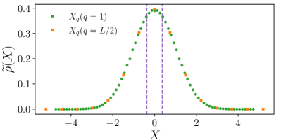
Figure 3: Eigenvalue distribution of the density wave operator $X_{q}$ for $q=1$ and $q=L/2$ for chain length $L=28$. The dashed lines indicate the coarse-graining window for $x=0$.

As an initial state we choose in the following

$$|\psi\rangle\sim e^{-\kappa X_{q}/2}|\psi_{R}\rangle,$$ (73)

where $|\psi_{R}\rangle$ is a random state with coefficients drawn from a zero-mean Gaussian distribution. Thus, $|\psi_{R}\rangle$ mimics an infinite temperature state, which makes optimal use of the available Hilbert space dimension. Moreover, $e^{-\kappa X_{q}/2}$ prepares the system out of equilibrium, where $\kappa$ is a perturbation strength. Below, we choose a moderate perturbation $\kappa=0.1$, but we have also checked results for different initial states corresponding to different temperatures and different perturbations and observed similar behaviour. These results are relegated to the supplemental material SM (2).

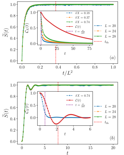
Figure 4: Time evolution of thermodynamic entropy for the longest (a) and shortest wave length (b) for different chain lengths $L$ as indicated in the plot. The time axis is rescaled in (a) because the relaxation time scales like $L^{2}$ for slow observables whereas it is system size independent for fast observables. Insets: Time evolution of correlation functions for $L=28$ as explained in the main text.

From what we said below Eq. (71) we expect that our theory works well for $q=1$ but not for $q=L/2$. A first indicator for this is shown in Fig. 4, where we plot for better comparison the rescaled thermodynamic entropy

$$\tilde{S}(t)\equiv\frac{S(t)-S(0)}{S(\infty)-S(0)}$$ (74)

with $S(\infty)=\ln D$. We see that it increases monotonously for $q=1$, as predicted by Eq. (67), whereas it clearly violates Eq. (67) for $q=L/2$. This violation also does not seem to become smaller for larger system size. Moreover, the vertical red dashed line in the figures indicates the thermalization time $t_{\text{th}}$ for comparison. It is defined to be the time by which the rescaled expectation value $\langle\tilde{X}_{q}\rangle$ for the case $L=28$, defined similar to Eq. (74), decayed to 1 percent and stayed below this threshold afterwards. Since $t_{\text{th}}$ fluctuates in each realization, we averaged it over 10 different initial states.

To further investigate the slowness of $X_{q}$, the insets of Fig. 4 show the behaviour of the correlation function ${\cal{C}}_{X}=\mbox{tr}\{\Pi_{0}(t)\Pi_{0}\}/\mbox{tr}\{\Pi_{0}\}$ as a function of time for $q=1$ and $q=L/2$ as well as for different coarse-graining sizes $\delta X$. Moreover, we also plot the correlation function ${\cal{C}}=\mbox{tr}\{X(t)X\}/\mbox{tr}\{X^{2}\}$ and the dotted purple vertical line indicates the microscopic evolution time scale $\pi/\Delta E$ (since we do not use a microcanonical energy window, $\Delta E$ here denotes the standard deviation of the energy spectrum). The insets thus demonstrate again that $X_{q}$ is slow for $q=1$ but not for $q=L/2$. Moreover, we confirm that projectors are slower for coarser coarse-grainings as derived in Appendix B.

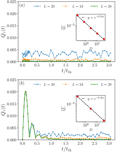
Figure 5: Time evolution of the quantum term for $q=1$ (a) and $q=L/2$ (b). The insets show a log-log plot of a suitable time-average as a function of the dimension $D$.

Next, we consider in Fig. 5 the influence of the quantum part $Q$ on the dynamics as discussed in Sec. III. Specifically, we consider the quantity

$$Q_{\tau}(t)=\sum_{x}\left|\sum_{y\neq z}\text{tr}\{\Pi_{x}U_{\tau}\Pi_{y}\rho(t)\Pi_{z}U_{\tau}^{\dagger}\}\right|$$ (75)

for $\tau=t_{\text{th}}/30$, which is a time scale at which nonequilibrium phenomena happen. Now, in Sec. III we have argued that the term inside the absolute value should be very small for slow observables and estimated that it scales like $D^{-\alpha}$ with unknown $\alpha$. The smallness of $Q_{\tau}(t)$ for a slow observable becomes immediately obvious from Fig. 5, whereas it is an order of magnitude larger for the fast case for times up to $t_{\text{th}}/2$. However, we also see that $Q_{\tau}(t)$ fluctuates for all times. To better check the scaling and to smooth out fluctuations, we consider the time average

$$\overline{Q_{\tau}}=\frac{1}{t_{f}-t_{\text{th}}}\int^{t_{f}}_{t_{\text{th}}}dtQ_{\tau}(t),$$ (76)

where the integral is taken in the time interval during which $Q_{\tau}$ has approximately reached a steady value. The insets of Fig. 5 reveal that the scaling exponent is $\alpha\approx 0.56$ for the slow case. Interestingly, also the fast case obeys a scaling law for times $t\geq t_{\text{th}}$ with a smaller exponent $\alpha\approx 0.42$. This indicates that classicality could be a universal feature for any coarse observable of a nonintegrable many-body system for not too small times. Moreover, as in Fig. 4 we see that for the fast case the initial violation of classicality does not seem to become smaller for larger system sizes. This challenges the universal validity of the penultimate paragraph of Sec. II.2, where we stated that sums of local observables tend to become slow for $L\rightarrow\infty$. Although we are numerically far away from the $L\rightarrow\infty$ case we have no direct explanation for that behaviour.

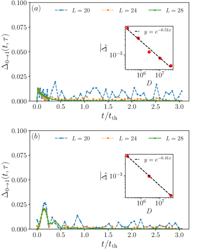
Figure 6: Check of LDB for $\Theta=K_{z}$ for $q=1$ (a) and $q=L/2$ (b). The insets show a log-log plot of a suitable time average as a function of the dimension $D$. Note that we only check the LDB condition in case (b) if $L=4k$ (with $k\in\mathbb{N}$) because it turns out that the $x=0$ subspace is empty if $L=4k+2$ (recall that we restricted the dynamics to the zero magnetization subspace).

Finally, we turn to the condition of LDB and consider the quantity

$$\Delta_{0\rightarrow 1}(t,\tau)=\left|\frac{{V}_{1}R_{1,0}(t,\tau)}{{V}_{2}R^{\text{TR}}_{0,1}(t,\tau)}-1\right|.$$ (77)

Here, $R_{x,y}(t,\tau)=\mbox{tr}\{\Pi_{x}U_{\tau}\rho_{y}(t)U_{\tau}^{\dagger}\}$ is the rate to jump from $y$ to $x$. To define $R^{\text{TR}}_{y,x}(t,\tau)$ we need to introduce a time-reversal operator $\Theta$. As discussed in Sec. V.1, multiple choices are conceivable.

We first choose $\Theta=K_{z}$, where $K_{z}$ denotes complex conjugation in the local $s_{z}$ basis. For that choice we find $\Theta(s_{x},s_{y},s_{z})\Theta^{-1}=(s_{x},-s_{y},s_{z})$ and easily confirm that both the Hamiltonian and observable are symmetric and hence $R^{\text{TR}}_{y,x}(t,\tau)=R_{y,x}(t,\tau)$. In Fig. 6 we plot $\Delta_{0\rightarrow 1}(t,\tau)$ for the slow and fast case with $\tau=t_{\text{th}}/30$ again. Furthermore, to check the scaling, the insets show again the time-average

$$\overline{\Delta_{\tau}}=\frac{1}{t_{f}-t_{\text{th}}}\int_{t_{\text{th}}}^{t_{f}}\Delta_{0\rightarrow 1}(t,\tau).$$ (78)

It is evident that LDB is well satisfied for the slow observables at all times. Also for the fast observable LDB is well satisfied for most times, only initially some slight violations do not vanish even with increasing system size. We attribute this behaviour to the particular choice of initial state in Eq. (73), which is very smoothly spread out over all microstates and thus looks quite “typical” even for the fast observable. The situation changes for different initial states as studied in the supplemental material SM (2).

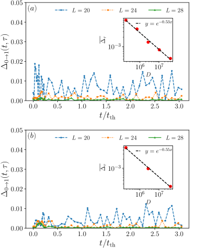
Figure 7: The same as Fig. 6 but with $\Theta$ defined in Eq. (79).

As a second choice we consider

$$\Theta=\exp\left[\frac{i\pi}{2}(\sigma_{y}^{(1)}+\dots+\sigma_{y}^{(L)})/2\right]K_{z}$$ (79)

for which we find $\Theta(s_{x},s_{y},s_{z})\Theta^{-1}=-(s_{x},s_{y},s_{z})$. Since angular momentum is odd under time-reversal in classical mechanics, this could be considered the “conventional” choice. In this case we find $\Theta X_{q}\Theta^{-1}=-X_{q}$ whereas $H$ is still symmetric under time-reversal. From what we said about the eigenvalues and eigenvectors above Eq. (72), we infer that $\Theta\Pi_{x}\Theta^{-1}=\Pi_{-x}$ and hence $R^{\text{TR}}_{y,x}(t,\tau)=R_{-y,-x}(t,\tau)$. This LDB condition is different from the previous one and we check its validity in Fig. 7. The conclusions are, however, the same as the plots look very similar to Fig. 6.

To conclude, we clearly see the emergence of classicality and LDB for the pure state dynamics of a slow observable of a non-integrable many body system. Instead, for the fast observable classicality does not hold for transient times, whereas LDB is quite well satisfied due to the smoothness of the initial state. These results, together with the additional results presented in the supplemental material SM (2), firmly support our main ideas.

VII Further Discussion

VII.1 Multiple observables

While we argued that slowness is a necessary condition for classicality, Markovianity and LDB, we have also collected some evidence that it is not sufficient. In particular, it was important that the state vector explores the available Hilbert space in a seemingly “unbiased” fashion. Here, we further discuss the subtlety of slowness, mostly from the perspective of multiple observables. Certainly, more research is required in the future.

To begin with, we emphasize once more the importance to take all strictly conserved quantities into account. In most applications this will be energy and particle number, but extensions to other non-commuting are desirabe too Murthy et al. (2022). In any case, if one misses one of those conserved quantities, it is clear that one can not assume the state to spread equally over the subspace ${\cal{H}}_{x}$ corresponding to a macrostate $x$.

Next, let $X,Y,Z,\dots$ be slow observables that are not conserved. If these observables mutually commute, our results carry over immediately by replacing ${\cal{H}}_{x}$ with ${\cal{H}}_{x,y,z,\dots}$ provided the dimension of these subspaces remains large enough. Examples of this kind include, e.g., the local energy and particle number of an open system.

The situation is more complicated if the observables do not commute. To examine this situation, let us first assume that their mutual commutator is small, i.e., $\|[X,Y]\|\ll\|X\|\|Y\|$. Now, if there are only two such slow observables, then it is possible to construct approximations $X^{\prime}$ and $Y^{\prime}$ to $X$ and $Y$ that satisfy $[X^{\prime},Y^{\prime}]=0$ Lin (1995); Hastings (2009) and our approch can be applied to $X^{\prime}$ and $Y^{\prime}$. We believe this covers a large class of relevant situations in statistical mechanics, but it is interesting to ask what happens beyond.

If there are more than two observables that approximately commute, von Neumann thought that it is still possible to approximate them by commuting observables von Neumann (1929, 2010). Also van Kampen assumed that the issue of non-commutativity can be overcome by coarse-graining, i.e., that the quantum uncertainty is drowned by the experimental measurement error Van Kampen (1954). We now know that three or more approximately commuting observables can not be approximated by commuting observables in general Choi (1988). However, observables of macroscopic systems that are sums of local observables, and thus of particular relevance to statistical mechanics, can be approximated by commuting observables Ogata (2013). An explicit construction for the subspaces of the corresponding macrostates was given in Ref. Halpern et al. (2016), which could be used to extend the present theory.

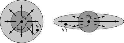
Figure 8: Two local regions of the sphere in Fig. 1 with respect to the effective observable mentioned in the text and exemplary trajectories $\psi_{0}\mapsto\psi_{t}$. Our theory is applicable whenever a small $\epsilon$-ball of initial states around $\psi_{0}$ (dark shaded region) approximately explores the sphere in an isotropic fashion on a time-scale $t$ obeying $\tau\gg t\gg\Delta E^{-1}$ as shown on the left. In contrast, on the right there is a strong preference to move in a horizontal direction, indicating that there is another slow observable associated to slow motion in the vertical direction that need be accounted for.

What remains is the case of multiple slow observables that are “strongly” non-commuting, although we are not aware of any example in statistical mechanics that clearly demonstrates the necessity to consider that case. However, it is a legitimate point of view to claim that, even if an experimenter attempts to measure multiple observables (whether commuting or not), the resulting transformation on the system is mathematically always described by one set of projectors (or more generally a set of positive operator-valued measures) belonging to one effective observable. While it might be hard to infer that effective observable, it only matters that it is slow. Our theory will work for this effective observable whenever the dynamics in this basis is approximately isotropic on the sphere introduced in Sec. II.1 because then the state vector explores the space in an unbiased way from a coarse-grained point of view, which allows to use typicality arguments. This intuition is sketched in Fig. 8.

Unfortunately, it is unknown to us whether there are generic arguments that explain whether an observable gives rise to a behaviour as illustrated on the left or on the right of Fig. 8. Some intuition on this question can be gained from Ref. Knipschild and Gemmer (2020), where “strange relaxation dynamics” were generated by choosing an envelope function $F(\omega)$ in the ETH ansatz, which is very different from a step function (as assumed in Sec. III.1), e.g., a step function modulated by a cosine. As long as this observable remains narrowly banded, it would still qualify as slow. However, the unusual modulation with a cosine function causes non-Markovian dynamics Knipschild and Gemmer (2020). From the perspective of the present paper, we would say that the cosine modulation preferably selects certain energy coherences over others such that the dynamics of the microstate no longer appears isotropic or unbiased.

VII.2 Symmetric part of the rates

This paper argued in great generality that the dynamics of a slow and coarse observable (modulo the difficulties mentioned in the previous section) is given by a classical Markov process describable by a master equation with rates $R_{x,y}(\psi_{y})$, which are almost constant as a function of the microstate $\psi_{y}$. This implied that their asymmetric part obeys LDB and one possible parametrization of the rates is therefore $R_{x,y}(\psi_{y})=S_{xy}\sqrt{V_{x}/V_{y}}$, where the symmetric part $S_{xy}=S_{yx}$ remained unspecified.

It is not surprising that it turns out that our methods employed so far are too general to draw any decisive conclusions about the symmetric part $S_{xy}$. It is strongly model-dependent and contains all the informaton about the nature of the system, its precise interactions, whether it is dominated by fast or slow transitions, etc. The symmetric part therefore can only be inferred by specifying more details about the model, and additional approximation schemes such as perturbation theory are likely necessary to proceed analytically. Since the numerous models and techniques are well covered in the existing literature, we do not follow down this path here.

However, at least one property of $S_{xy}$ can be inferred rather easily and we briefly sketch how to do this here. This property concerns the topology formed by the network of macrostates $x$. In fact, we can view a master equation description as a graph, where the vertices are formed by the states $x$, and two states $x$ and $y$ are connected by an edge whenever $S_{xy}\neq 0$. Thus, while we are not able to fix or estimate any finite value of $S_{xy}$, we can at least decide whether $S_{xy}\neq 0$ or not, which already provides valuable information about the concrete physical behaviour of the system.

To do so, we follow Ref. Hamazaki (2022) and directly cast the von Neumann equation $\partial_{t}\rho(t)=-i[H,\rho(t)]$ as a continuity equation for the probabilities $p_{x}(t)$. Namely, we find

$$\frac{d}{dt}p_{x}(t)=\sum_{y(\neq x)}J_{x,y},$$ (80)

where $J_{x,y}\equiv-i\mbox{tr}\{H_{xy}\rho_{yx}(t)-\rho_{xy}(t)H_{yx}\}$ is a probability current from $y$ to $x$ (with $H_{xy}\equiv\Pi_{x}H\Pi_{y}$ and $\rho_{xy}=\Pi_{x}\rho\Pi_{y}$). Thus, we see that $S_{x,y}$, and hence $R_{x,y}$, is non-zero only if $J_{x,y}\neq 0$, which implies that $H_{xy}$ must not be the null operator. Now, while it is hard to compute the transition rates $R_{xy}$ or probabilities $P_{x|y}(\tau)$ directly, it is typically easy to know whether $H_{xy}=0$ or not.

For instance, consider two weakly coupled subsystems $A$ and $B$ exchanging particles (say, electrons) with each other. Most microscopic interaction Hamiltonians will only contain terms proportional to $c_{A}c_{B}^{\dagger}+c_{B}c_{A}^{\dagger}$, where $c_{A/B}^{\dagger}$ ($c_{A/B}$) in the creation (annihilation) operator of an electron in $A/B$. Thus, we see that a coarse-graining of the particle number operator of $A$ with states $n\in\mathbb{N}$ describing $n$ electrons in $A$ will give rise to a master equation in form of a birth-and-death process, where only neighbouring probabilities are connected, i.e., $R_{n,n^{\prime}}=0$ if $|n-n^{\prime}|>1$. If the subsystems are superconductors, then the interaction Hamiltonian also contains a term porportional to $(c_{A})^{2}(c_{B}^{\dagger})^{2}+(c_{B})^{2}(c_{A}^{\dagger})^{2}$, which implies that also $R_{n,n+2}\neq 0$. In this way, we can infer the structure of the graph describing the dynamics of $p_{x}(t)$.

For the future it seems worth to explore methods to quantiatively estimate the symmetric part $S_{xy}$ of the rates without using perturbation theory, for instance, by using tools from quantum speed limits Mandelstam and Tamm (1945); Deffner and Campbell (2017); Hamazaki (2022) or recent results on thermalization times Goldstein et al. (2013); García-Pintos et al. (2017); de Oliveira et al. (2018); Wilming et al. (2018); Nickelsen and Kastner (2019); Heveling et al. (2020); Simenel et al. (2020).

VIII Conclusions

It is a fact that many natural processes are well approximated by classical Markov processes obeying local detailed balance. While this is a curse (or welcome challenge) for many researchers, for instance, those who are interested in building a large scale quantum computer or finding quantum effects in thermodynamics, it is also a blessing for many other researchers because it greatly simplifies their life and, in fact, it does not sound too speculative that stability, predictability and some reduced (but not too low) complexity are important ingredients for the existence of intelligent life itself.

It is also a fact that the repeated randomness assumption—i.e., the repeated use of the equal-a-priori-probability postulate or the maximum entropy principle—explains the emergence of classicality, Markovianity and local detailed balance. Yet, this assumption is at odds with unitary quantum mechanics (or phase space preserving classical mechanics), and no satisfactory microscopic explanation has been put forward so far.

Based on the intuitive (and already previously used) picture of a slow and coarse observable, we provided various estimates, mathematical theorems and numerical simulations that justify the repeated randomness assumption for the dynamics of a pure state of an isolated nonintegrable many-body system. Importantly, our approach is not in conflict with unitary quantum mechanics.

We also find it noteworthy that our approach did not make use of common concepts and approximations. For instance, we did not use Nakajima-Zwanzig projection operator techniques, repeated interaction schemes, Born approximations, perturbation theory, various sorts of Markov assumptions, secular approximations, among others, which are often hard to control and justify microscopically.

Nevertheless, the price to pay was to accept an intuitive but technically subtle notion of slowness, in particular with respect to the question whether the microscopic state diffuses in an unbiased or isotropic way from a coarse perspective. We believe, however, that it was worth to pay this price for the unifying perspective we have got on problems that are studied in many different branches of statistical mechanics.

Conceptually, our research offers a shift in perspective for the investigation of how classicality arises from quantum mechanics. Central to our approach is chaos in an isolated many-body system and a definition of classicality based on multi-time probabilities (Kolmogorov consistency), instead of focusing on the dynamics of an open quantum system as done in the decoherence approach Zurek (2003); Joos et al. (2003); Schlosshauer (2019). Importantly, our approach is not in conflict with environmentally induced decoherence, yet we believe we cannot agree with the statement of Zeh, one of the pioneers of the decoherence approach, that “all attempts to describe macroscopic objects quantum mechanically as being isolated […] were thus doomed to fail” Zeh (2007). It is an interesting future prospect to connect these approaches to semiclassical methods based on a stationary phase approximation of the Feynman path integral Berry (2009); Braun (2001); Garbaczewski and Olkiewicz (2002); Padmanabhan (2015). Interestingly, the semiclassical limit for Hamiltonians with a classically chaotic limit is problematic due to a rapid smearing out of the wave function over phase space, which is usually addressed by using environmentally induced decoherence Zurek and Paz (1994); Calzetta (2012). How this fits together with our picture is at present unclear to us.

Furthermore, we provided a systematic justification of the validity of the Markov approximation, which does not rely on an initial ensemble average that has the potential to wash out already many non-Markovian effects. Moreover, we stressed the important role played by the observable (and not only the Hamiltonian) for the question of (non-)Markovianity.

Among the more technical insights, we want to highlight our idea to account for correlations between initial nonequilibrium states and the pseudorandom coefficients in the ETH ansatz (Sec. III.1) and the observation that multiple local detailed balance relations can exist for the same setup (Secs. V.1 and VI).

It is further worth to comment on how breaking of time-reversal symmetry emerges in our framework given that our approach does not use any of the common mechanisms to break it: there are no special initial or repeated ensemble averages and both, the ETH and typicality, are arguments that are time-symmetric. In fact, our approach leaves room for a time-symmetric picture because we have “only” shown that it is overwhelmingly more likely to evolve into the direction of an increasing entropy gradient. Applying a time-reversal operator to a microstate along this dynamics would indeed provide an example for one of those atypical nonequilibrium states for which the master equation does not apply. However, since entropy is proportional to the volume of the macrostates and since these volumes grow very quickly the closer we are to equilibrium, it is very unlikely to accidentially hit such an atypical state. Of course, this general picture complies well with Boltzmann’s intuition about the second law Lebowitz (1993).

Our results also suggest that the repeated randomness assumption quickly breaks down for observables that are neither slow nor coarse. In that regime, it seems that not many universal features remain, an exception being the laws of thermodynamics including fluctuation theorems (see Refs. Seifert (2012); Schaller (2014); Peliti and Pigolotti (2021); Strasberg (2022) and references therein). This makes the (thermo)dynamic description of such processes very rich in variety, but also extremely hard to describe with common principles.

Finally, our work leaves much room for future research, for instance, related to classicality, decoherence and interpretations of quantum mechanics, or related to the subtle notion of slowness, possible refinements thereof and systematic correction terms for observables that are a little faster and finer than the present observables but not too fast and fine.

Acknowledgements

Discussions with Josh Deutsch, Mark Srednicki and Nicole Yunger Halpern are gratefully acknowledged. PS further acknowledges collaboration and discussion with John Goold, Mark Mitchison and Kavan Modi on a related project (unpublished). PS and AW acknowledge financial support from the European Commission QuantERA grant ExTRaQT (Spanish MICINN project PCI2022-132965), by the Spanish MINECO (project PID2019-107609GB-I00) with the support of FEDER funds, the Generalitat de Catalunya (project 2017-SGR-1127), by the Spanish MCIN with funding from European Union NextGenerationEU (PRTR-C17.I1) and the Generalitat de Catalunya. PS is financially supported by “la Caixa” Foundation (ID 100010434, fellowship code LCF/BQ/PR21/11840014). AW is furthermore supported by the Alexander von Humboldt Foundation, as well as the Institute of Advanced Study of the Technical University Munich. JW and JG are supported by the Deutsche Forschungsgemeinschaft (DFG) within the Research Unit FOR 2692 under Grant No. 397107022 (GE 1657/3-2).

Appendix A Bandedness implies small commutator

For any operator $A$ the operator norm is defined as $\|A\|=\sup_{{\langle{\psi|\psi}\rangle}=1}\sqrt{{\langle{\psi|A^{\dagger}A|\psi}\rangle}}$ and equals the maximum eigenvalue (in absolute value) for normal operators satisfying $AA^{\dagger}=A^{\dagger}A$. For simplicity we can will assume that the groundstate energy is zero, $E_{0}=0$, and that the largest eigenvalue of $H$ satisfies $E_{D}=1$. This implies $\|H\|=1$.

A straightforward calculation reveals that

$$\begin{split}&{\langle{\psi|[H,X]^{\dagger}[H,X]|\psi}\rangle}\\ &=\sum_{k,\ell,m}c_{k}^{*}c_{m}X_{k\ell}X_{\ell m}(E_{m}-E_{\ell})(E_{k}-E_{\ell}).\end{split}$$ (81)

Now, if $X$ is banded, the sum over $k$ and $m$ can be restricted to ‘nearby’ values around $\ell$ and we can bound the energy differences by the band width $\delta E$:

$$\begin{split}\text{Eq.\leavevmode\nobreak\ (\ref{eq operator norm commutator})}&\leq\delta E^{2}\sum_{k,\ell,m}c_{k}^{*}c_{m}X_{k\ell}X_{\ell m}\\ &=\delta E^{2}{\langle{\psi|X^{\dagger}X|\psi}\rangle}.\end{split}$$ (82)

Our assumptions $\|H\|=1$ and that $X$ is narrowly banded imply $\delta E\ll 1$. Since the previous equation holds for any state $|\psi\rangle$, we conclude

$$\|[H,X]\|\leq\delta E\|X\|\ll\|X\|.$$ (83)

Appendix B Proof of bandedness of projectors

We consider an arbitrary observable $A$ and its spectral decomposition $A=\sum_{a=1}^{M}\lambda_{a}\Pi_{a}$. We like to construct a function $f_{a}$ that satisfies $f_{a}(A)=\Pi_{a}$. It can be shown that this is the case if $f_{a}$ satisfies $f_{a}(\lambda_{b})=\delta_{ab}$ by looking at $f_{a}(A)|\psi\rangle$ for an arbitrary $|\psi\rangle$ expanded in the eigenbasis of $A$. Moreover, it is clear that the function $f_{a}(x)=c\prod_{b(\neq a)}(x-\lambda_{b})$ satisfies $f_{a}(\lambda_{b})=\delta_{a,b}$ if the constant $c$ is chosen such that $f_{a}(\lambda_{a})=1$. Thus, we see that $f_{a}$ is a polynomial of degree $M-1$.

This implies that, if $A$ is banded, then so is $\Pi_{a}$, although it is not as narrowly banded. Suppose the $A_{k\ell}$ are distributed around the diagonal according to a Gaussian with variance $\sigma^{2}$, then the elements $(\Pi_{a})_{k\ell}$ are distributed around the diagonal with variance $(M-1)\sigma^{2}$, i.e., the standard deviation is approximately $\sqrt{M}\sigma$.

Appendix C Supplemental Material

We present further numerical results about density waves in the XXZ spin chain, in particular for different initial states and different coarse-graining widths. We consistently find that classicality and local detailed balance (LDB) holds for slow observables, though their scaling $D^{-\alpha}$ with the dimension can be different from the $\alpha=0.5$ case in the main text. In contrast, pronounced violations are observed for fast observables. Moreover, we find the counterintuitive result that LDB can sometimes be better satisfied for finer (instead of coarser) observables for short times, and explain it with the special structure of the observable. Finally, we also briefly study the different setup of energy exchanges between two spin chains and confirm our main conclusions also there.

C.1 Results for other initial states

C.1.1 Results for initial states far from equilibrium

In this section, we consider an initial state as in Eq. (79) but for $\kappa=0.3$ (instead of $\kappa=0.1$).

The influence of the quantum part $Q_{\tau}(t)$ are shown in Fig. 9. Similar to the main text, the quantum part for the slow observable is small and scales like $D^{-\alpha}$ with $\alpha=0.52$. In contrast, for the fast observable the quantum part is much larger for times up to $t_{\text{th}}/2$ and roughly three times larger than in Fig. 4, suggesting that classicality does not hold far from equilibrium for fast observables. However, for times $t\geq t_{\text{th}}/2$ a scaling with $\alpha=0.37$ is again confirmed.

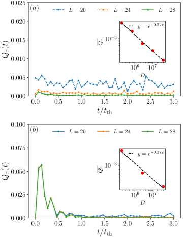
Figure 9: Time evolution of the quantum term $q=1$ (a) and $q=L/2$ (b) for coarse-graining width $\delta X=2.0$ for far-from-equilibrium initial states with $\kappa=0.3$. The insets show a log-log plot of a suitable time-average as a function of the dimension $D$ of the total Hilbert space.

Next, we check the condition of LDB, which involves a technical subtlety. Recall that LDB was derived for the dynamics contained inside a microcanonical energy shell. In Sec. VI of the main text, we already relaxed that condition as we considered the entire Hilbert space. This was possible because the coefficients of a slightly perturbed initial state with $\kappa=0.1$ are well distributed across the entire Hilbert space, whose spectrum closely resembles a Gaussian distribution with zero mean, thus effectively corresponding to an infinite temperature state (see Fig. 10 for the spectrum). However, for states far from equilibrium as considered here the coefficients in the energy eigenbasis are far from being equally distributed throughout the whole Hilbert space, so effectively, we are restricted to a different Hilbert space. Thus, instead of the dimension of the whole subspace ($V_{x}$), we need to consider the effective volume

$$\widetilde{V}_{x}=\pi_{x}D,$$ (84)

which is dependent on the equilibrium state probabilities $\pi_{x}$. In our numerical simulations, the effective dimension $\widetilde{V}_{x}$ is calculated as

$$\widetilde{V}_{x}=\frac{1}{t_{f}-t_{\text{th}}}\int_{t_{\text{th}}}^{t_{f}}\text{tr}(\rho(t)\Pi_{x})dt.$$ (85)

Since all initial states considered in this section are far from equilibrium, the effective dimension will be used throughout this section to check the condition of LDB.

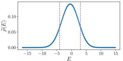
Figure 10: Rescaled density of state $\widetilde{{\rho}}(E)=\rho(E)/D$ for the XXZ model for $L=28$. The dashed line indicate the microcanonical window considered in Sect.C.1.3 .

Similar to the results for the near-equilibrium initial state, one can see from Fig. 11 that LDB is well satisfied for slow observables also for the far-from-equilibrium intial state, and obeys a scaling law with $\alpha=0.47$. In contrast, initial violations up to $t_{\text{th}}/2$ (roughly twice as large as in Fig. 5) are clearly visible for the fast observable, and the scaling is notably worse with $\alpha=0.13$.

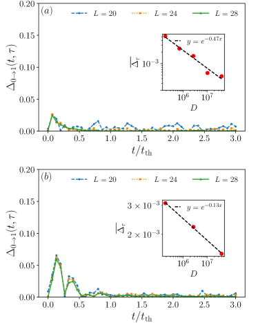
Figure 11: Check of LDB for $\Theta=K_{z}$ for $q=1$ (a) and $q=L/2$ (b) for coarse-graining width $\delta X=0.74$ for far-from-equilibrium initial states with $\kappa=0.3$. The insets show a log-log plot of time average as a function of the dimension $D$ of the total Hilbert space.

C.1.2 Results for initial states distributed in the two largest subspace

In this section, we consider a different kind of initial state. It is initially distributed only in the two subspace $I_{0}$ and $I_{1}$ defined in Eq. (78) and can be written as

$$|\psi\rangle=\sqrt{p_{0}}\Pi_{0}|\psi_{R}^{0}\rangle+\sqrt{p_{1}}\Pi_{1}|\psi_{R}^{1}\rangle,$$ (86)

where $|\psi^{1,2}_{R}\rangle$ are random states and $p_{0}=\frac{1+\delta p}{2},\ p_{1}=\frac{1-\delta p}{2}$.

Starting with the investigation of classicality again, one can see from Fig. 12 that—in unison with our main claim—for slow observables the quantum part $Q_{\tau}(t)$ is very small. It is interesting to note, however, that the scaling with $\alpha=0.32$ is worse compared to the previous examples, and the detailed reasons for this behaviour remain to be understood. Moreover, we observe very strong violations of classicality for the fast observable up to times $t_{\text{th}}/2$. Afterwards, a similar scaling law with $\alpha=0.26$ is observed.

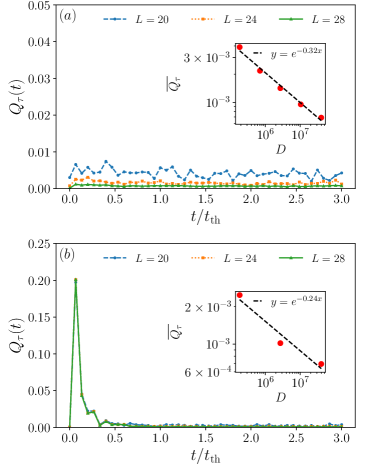
Figure 12: Time evolution of the quantum term $q=1$ (a) and $q=L/2$ (b) for coarse-graining width $\delta X=0.74$ for initial states in Eq. (86) for $\delta p=0.2$. The insets show a log-log plot of a suitable time-average as a function of the dimension $D$ of total Hilbert space.

Next, we check the condition of LDB in Fig. 13. The general behavior of it for both the slow and fast observable case is similar to what we found before. However, for the fast case strong violations of LDB are found at early times indicating that slowness is crucial for LDB to hold out of equilibrium, which was less visible in Fig. 5 and 6. The probable reason for that is that the initial state considered in the main text is close to a fully mixed state with respect to every coarse-grained subspace. As a result, the state may still stay close to typical states during the time evolution, even for the fast observable. Instead, the state in Eq. (86) considered here is only fully mixed in two subspaces, so during transient times it is more likely to evolve into atypical states while “exploring” new subspaces. Finally, after some transient time, LDB is also well satisfied for the fast case, but with a clearly different scaling ($\alpha=0.24$) compared to the slow case ($\alpha=0.47$).

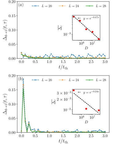
Figure 13: Check of LDB for $\Theta=K_{z}$ for $q=1$ (a) and $q=L/2$ (b) for coarse-graining width $\delta X=0.74$ initial states in Eq. (86) for $\delta p=0.2$. The insets show a log-log plot of time average as a function of the dimension $D$ of total Hilbert space.

In addition to what we have studied previously, we now also consider the influence of the coarse-graining width $\delta X$ on LDB for slow observables. To this end, besides the previously considered choice of $\delta X=0.74$, we also check LDB for finer coarse-grainings with $\delta X=0.37$ and $\delta X=0.18$. Figure 14 displays the results for the largest system size with $L=28$. Remarkably, we observe the counterintuitive results that LDB is better satisfied for finer coarse-grainings for short times. This is in contrast to what we should expect based on a naive application of Levy’s Lemma. The reason for that can be understood by considering the interconnection of microstates $|\textbf{z}\rangle$ belonging to the same coarse-grained space $I_{x}$. The dynamics on these states can be viewed as a network, where an edge connects two microstates $|\textbf{z}\rangle$ and $|\textbf{z}^{\prime}\rangle$ if the Hamiltonian creates an overlap between the two: $\langle\textbf{z}|H|\textbf{z}^{\prime}\rangle\neq 0$. Now, since the Hamiltonian $H$ in Eq. (76) contains only two-body interactions, many pairs of microstates in a given coarse-grained space $I_{x}$ are not directly connected by a single edge. This implies that there is not only a slow time scale associated to the evolution of the observable $X$ (associated to changes between subspaces $I_{x}$), but there is also a relatively slow time scale associated to changes between microstates in the same subspace. This implies that, if a state starts to explore a new subspace, it takes some time until it looks typical (i.e., evenly smeared out over different microstates) in that subspace. But it is precisely this “smearing out” over different microstates within a given subspace that justifies the Haar random average in the application of Levy’s Lemma, and this smearing out takes longer for larger subspaces, i.e., for coarser coarse-grainings. This is exactly what is observed in Fig. 14, which further shows how subtle the notion of a coarse and slow observable is as the interconnection of the network of microstates plays a central role. Moreover, note that this behaviour can not be observed for the initial state considered in the main text because this state is already well smeared out over all microstates.

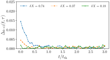
Figure 14: Check of LDB for $\Theta=K_{z}$ for $q=1$ for different coarse-graining width $\delta X=0.74,0.37,0.18$ for initial states in Eq.(86) for $\delta p=0.2$, with the system size $N=28$.

C.1.3 Results for initial states restricted to energy window

In this section, we consider yet another initial state which is restricted to a microcanonical energy window as sketched in Fig. 10. It has the following form

$$|\psi\rangle\sim\Pi_{E,\Delta E}e^{-\kappa{X_{q}/2}}|\psi_{R}\rangle,$$ (87)

where $|\psi_{R}\rangle$ is a random state drawn from a Gaussian distribution, and

$$\Pi_{E,\Delta E}=\sum_{E_{k}\in[E-\frac{\Delta E}{2},E+\frac{\Delta E}{2}]}|E_{k}\rangle\langle E_{k}|,$$ (88)

with $E_{k}$ and $|k\rangle$ being the eigenvalue and eigenstate of the Hamiltonian. Here the center of the energy window is chosen according to the canonical (inverse) temperature $\beta$ (here we only consider the infinite temperature case $\beta=0$) by the following equation

$$E=\frac{\text{tr}(e^{-\beta H}H)}{\text{tr}(e^{-\beta H})}.$$ (89)

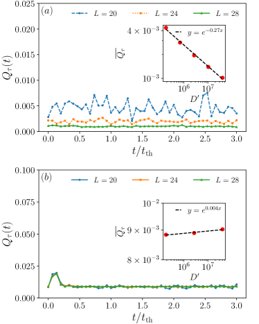
Figure 15: Time evolution of the quantum term for $q=1$ (a) and $q=L/2$ (b) for coarse-graining width $\delta X=0.74$ for initial state in a microcanonical energy window corresponding to infinite temperature $\beta=0$. The energy width $\Delta E$ is chosen to be $\Delta E=3\sqrt{L/20}$. The insets show a log-log plot of a suitable time-average as a function of the dimension $D^{\prime}$ of the microcanonical energy shell.

One can see from Fig. 15 that for the slow observable the quantum part $Q_{\tau}(t)$ is small for all times, but obeys a weaker scaling law with $\alpha=0.27$ (similar to Fig. 12) compared to the $\alpha\approx 0.5$ case of the main text. Moreover, violations for the fast observable are much stronger than for the slow observable, and no decay to zero is visible for long times. Nevertheless, we note that the violation of classicality is small compared to the maximum possible value of one.

In Fig. 16 we check the condition of LDB. Similar to the results shown in Fig. 15, LDB works well for the slow observable for almost all times except for small deviations until $t_{\text{th}}/4$. In contrast, for the fast observable LDB is still not satisfied even after the thermalziation time. The possible reason for both the persistent violation of classciality and LDB even after the thermalization time may be that—different from the slow observable where one has $[\Pi_{E,\Delta E},\Pi_{x}]\approx 0$—for fast observable the commutator $[\Pi_{E,\Delta E},\Pi_{x}]$ remains quite large. As a result, the state may still be highly atypical even after the thermalization time.

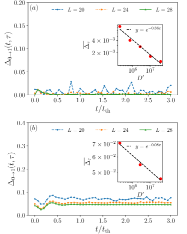
Figure 16: Check of LDB for $\Theta=K_{z}$ for $q=1$ (a) and $q=L/2$ (b) for coarse-graining width $\delta X=0.74$. The insets show a log-log plot of a suitable time average as a function of the dimension $D^{\prime}$ of the microcanonical energy shell.

C.2 Numerical results in coupled tilted field Ising model for canonical initial state

Besides the extensively studied XXZ model, we also briefly consider a different model, namely two coupled Ising models with tilted field. The Hamiltonian reads

$$H=H_{A}+H_{B}+\lambda H^{I}_{A}\otimes H^{I}_{B},$$ (90)

where

$$H_{A}=H_{B}=h_{x}\sum_{\ell=1}^{n}\sigma_{x}^{\ell}+h_{z}\sum_{\ell=1}^{n}\sigma_{z}^{\ell}+g_{z}\sum_{\ell=1}^{n}\sigma_{z}^{\ell}\sigma_{z}^{\ell+1},$$ (91)

and

$$H^{I}_{A}=H^{I}_{B}=\sigma^{n}_{z}.$$ (92)

Here $n=L/2$ is the length of the Ising chain with periodic boundaries, and we choose $h_{x}=1.0,\ h_{z}=0.5,\ g_{z}=1.0$. The eigenvalue and eigenstate of the two subsystems are denoted by

$$H_{A}|e_{\alpha}\rangle=e_{\alpha}|e_{\alpha}\rangle,\quad H_{B}|e_{\beta}\rangle=e_{\beta}|e_{\beta}\rangle.$$ (93)

The initial state we consider here is a product state of the canonical states of the two subsystems, obtained by makeing use of typicality,

$$|\psi\rangle=K(e^{-\beta_{A}H_{A}/2}|\psi_{R}^{A}\rangle)\otimes(e^{-\beta_{B}H_{B}/2}|\psi_{R}^{B}\rangle),$$ (94)

where $K$ is a normalization constant and $|\psi^{A,B}_{R}\rangle$ are Gaussian random states.

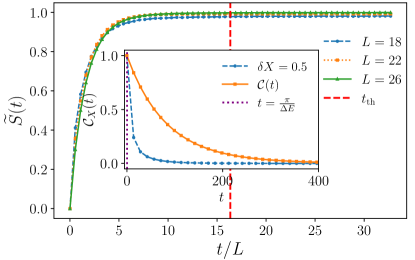
Figure 17: Time evolution of rescaled thermodynamic entropy $\widetilde{S}(t)$ for the energy difference operator for coupled Ising model as a function of $t/L$, for the initial state introduced in Eq. (94) for $\beta_{A}=0.1,\quad\beta_{B}=-0.1$ and $\lambda=0.5$. The time axis is rescaled as the relaxation time scales like $L$ for this observable. Insets: Time evolution of correlation functions for $L=26$ as explained in the main text.

Here we consider the energy difference operator

$$X=\frac{1}{\cal N}(H_{A}-H_{B})$$ (95)

where $\cal N$ is a normalization constant which fixes the second central moment of the operator to one. The projector of the coarse-grained eigenspaces can be written as

$$\Pi_{x}\equiv\sum_{e_{\alpha}-e_{\beta}\in[E-\frac{\delta X}{2},E+\frac{\delta X}{2}]}P_{\alpha\beta}$$ (96)

where

$$P_{\alpha\beta}=|e_{\alpha}\rangle\langle e_{\alpha}|\otimes|e_{\beta}\rangle\langle e_{\beta}|,$$ (97)

and $\delta X$ is the coarse-graining width (which is chosen as $\delta X=0.5$ in our numerical simulation).

First we show the result for the rescaled thermodynamics entropy $\widetilde{S}(t)$ defined in Eq. (80). It can be seen from Fig. 17 that $\widetilde{S}(t)$ increases monotonically, which is expected to be the case as the energy difference operator we consider here is a slow observable according to the inset of Fig. 17.

Next, we study the influence of the quantum part $Q_{\tau}(t)$ in Fig. 18(a). One can see that similar to the results we have in the XXZ model the quantum term is small for all times considered here, and its time average scales with $\alpha=0.49$ (close to the ideal scaling $\alpha=0.5$ estimated in Sec. III and in unison with the numerical results of the main text and of Fig. 9). In Fig. 18(b) the condition of LDB is checked, and one can see that after a slight deviation for times up to $t_{\text{th}}/4$ it stays close to zero, and it obeys again a scaling law with $\alpha=0.49$.

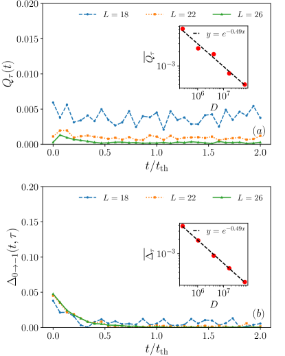
Figure 18: (a) $Q_{\tau}(t)$ versus $t/t_{\text{th}}$ and (b) $\Delta_{0\rightarrow-1}(t,\tau)$ versus $t/t_{\text{th}}$ in coupled Ising model for $\lambda=0.5$ and $\delta X=0.5$, for canonical initial state at temperature ($\beta_{A}=0.1,\quad\beta_{B}=-0.1$). The insets show a log-log plot of time average as a function of the dimension $D$ of the total Hilbert space.

References

- de Groot and Mazur (1984) S. R. de Groot and P. Mazur, Non-Equilibrium Thermodynamics (Dover Publications, New York, 1984).
- Zwanzig (2001) R. Zwanzig, Nonequilibrium Statistical Mechanics (Oxford University Press, New York, 2001).
- Nazarov and Blanter (2009) Y. V. Nazarov and Y. M. Blanter, Quantum Transport: Introduction to Nanoscience (Cambridge University Press, Cambridge, 2009).
- Stefanucci and van Leeuwen (2013) G. Stefanucci and R. van Leeuwen, Nonequilibrium many-body theory of quantum systems: A modern Introduction (Cambridge University Press, New York, 2013).
- Schaller (2014) G. Schaller, Open Quantum Systems Far from Equilibrium, Vol. 881 (Lect. Notes Phys., Springer, Cham, 2014).
- Strasberg (2022) P. Strasberg, Quantum Stochastic Thermodynamics: Foundations and Selected Applications (Oxford University Press, Oxford, 2022).
- Sekimoto (2010) K. Sekimoto, Stochastic Energetics, Vol. 799 (Lect. Notes Phys., Springer, Berlin Heidelberg, 2010).
- Seifert (2012) U. Seifert, “Stochastic thermodynamics, fluctuation theorems and molecular machines,” Rep. Prog. Phys. 75, 126001 (2012).
- Peliti and Pigolotti (2021) L. Peliti and S. Pigolotti, Stochastic Thermodynamics: An Introduction (Princeton University Press, Princeton, 2021).
- Bustamante et al. (2005) C. Bustamante, J. Liphardt, and F. Ritort, “The nonequilibrium thermodynamics of small systems,” Phys. Today 58, 43–48 (2005).
- Ciliberto (2017) S. Ciliberto, “Experiments in stochastic thermodynamics: Short history and perspectives,” Phys. Rev. X 7, 021051 (2017).
- van Kampen (2007) N. G. van Kampen, Stochastic Processes in Physics and Chemistry (North-Holland Publishing Company, Amsterdam, 3rd ed., 2007).
- Deutsch (1991) J. M. Deutsch, “Quantum statistical mechanics in a closed system,” Phys. Rev. A 43, 2046–2049 (1991).
- Srednicki (1994) M. Srednicki, “Chaos and quantum thermalization,” Phys. Rev. E 50, 888–901 (1994).
- Srednicki (1999) M. Srednicki, “The approach to thermal equilibrium in quantized chaotic systems,” J. Phys. A 32, 1163–1175 (1999).
- Rigol et al. (2008) M. Rigol, V. Dunjko, and M. Olshanii, “Thermalization and its mechanism for generic isolated quantum systems,” Nature 452, 854–858 (2008).
- Popescu et al. (2006a) S. Popescu, A. J. Short, and A. Winter, “Entanglement and the foundations of statistical mechanics,” Nat. Phys. 2, 754 – 758 (2006a).
- Ehrenfest and Ehrenfest (1911) P. Ehrenfest and T. Ehrenfest, “Begriffliche Grundlagen der statistischen Auffassung in der Mechanik,” (Teubner, Leipzig, 1911) pp. 3–90.
- Ehrenfest and Ehrenfest (1959) P. Ehrenfest and T. Ehrenfest, The Conceptual Foundations of The Statistical Approach in Mechanics, edited by translated by M. J. Moravcsik (Dover Pub., New York, 1959).
- Van Kampen (1954) N. Van Kampen, “Quantum statistics of irreversible processes,” Physica 20, 603–622 (1954).
- Gemmer et al. (2004) J. Gemmer, M. Michel, and G. Mahler, Quantum Thermodynamics, Vol. 784 (Lect. Notes Phys., Springer, Heidelberg, 2004).
- D’Alessio et al. (2016) L. D’Alessio, Y. Kafri, A. Polkovnikov, and M. Rigol, “From quantum chaos and eigenstate thermalization to statistical mechanics and thermodynamics,” Adv. Phys. 65, 239–362 (2016).
- Borgonovi et al. (2016) F. Borgonovi, F.M. Izrailev, L. F. Santos, and V. G. Zelevinsky, “Quantum chaos and thermalization in isolated systems of interacting particles,” Phys. Rep. 626, 1–58 (2016).
- Gogolin and Eisert (2016) C. Gogolin and J. Eisert, “Equilibration, thermalisation, and the emergence of statistical mechanics in closed quantum systems,” Rep. Prog. Phys. 79, 056001 (2016).
- Goold et al. (2016) J. Goold, M. Huber, A. Riera, L. del Rio, and P. Skrzypzyk, “The role of quantum information in thermodynamics – a topical review,” J. Phys. A 49, 143001 (2016).
- Deutsch (2018) J. M. Deutsch, “Eigenstate thermalization hypothesis,” Rep. Prog. Phys. 81, 082001 (2018).
- Mori et al. (2018) T. Mori, T. N. Ikeda, E. Kaminishi, and M. Ueda, “Thermalization and prethermalization in isolated quantum systems: a theoretical overview,” J. Phys. B 51, 112001 (2018).
- Bartsch and Gemmer (2009) C. Bartsch and J. Gemmer, “Dynamical Typicality of Quantum Expectation Values,” Phys. Rev. Lett. 102, 110403 (2009).
- Reimann (2018) P. Reimann, “Dynamical typicality of isolated many-body quantum systems,” Phys. Rev. E 97, 062129 (2018).
- Xu et al. (2022) X. Xu, C. Guo, and D. Poletti, “Typicality of nonequilibrium quasi-steady currents,” Phys. Rev. A 105, L040203 (2022).
- Gemmer and Michel (2006) J. Gemmer and M. Michel, “Finite quantum environments as thermostats: an analysis based on the Hilbert space average method,” Eur. Phys. J. B 53, 517–528 (2006).
- Breuer et al. (2006) H.-P. Breuer, J. Gemmer, and M. Michel, “Non-Markovian quantum dynamics: Correlated projection superoperators and Hilbert space averaging,” Phys. Rev. E 73, 016139 (2006).
- Gemmer and Breuer (2007) J. Gemmer and H.-P. Breuer, “Projection operator techniques and Hilbert space averaging in the quantum theory of nonequilibrium systems,” Eur. Phys. J. 151, 1–12 (2007).
- Hahn et al. (2020) N. Hahn, T. Guhr, and D. Waltner, “Hilbert space average of transition probabilities,” Phys. Rev. E 101, 062135 (2020).
- Reimann (2016) P. Reimann, “Typical fast thermalization processes in closed many-body systems,” Nat. Comm. 7, 10821 (2016).
- Balz and Reimann (2017) B. N. Balz and P. Reimann, “Typical Relaxation of Isolated Many-Body Systems Which Do Not Thermalize,” Phys. Rev. Lett. 118, 190601 (2017).
- Reimann and Dabelow (2019) P. Reimann and L. Dabelow, “Typicality of Prethermalization,” Phys. Rev. Lett. 122, 080603 (2019).
- Dabelow and Reimann (2020) L. Dabelow and P. Reimann, “Relaxation Theory for Perturbed Many-Body Quantum Systems versus Numerics and Experiment,” Phys. Rev. Lett. 124, 120602 (2020).
- Richter et al. (2020a) J. Richter, F. Jin, L. Knipschild, H. De Raedt, K. Michielsen, J. Gemmer, and R. Steinigeweg, “Exponential damping induced by random and realistic perturbations,” Phys. Rev. E 101, 062133 (2020a).
- Dabelow and Reimann (2021) L. Dabelow and P. Reimann, “Typical relaxation of perturbed quantum many-body systems,” J. Stat. Mech.: Theory and Experiment , 013106 (2021).
- Goldstein et al. (2013) S. Goldstein, T. Hara, and H. Tasaki, “Time scales in the approach to equilibrium of macroscopic quantum systems,” Phys. Rev. Lett. 111, 140401 (2013).
- García-Pintos et al. (2017) L. P. García-Pintos, N. Linden, A. S. Malabarba, A. J. Short, and A. Winter, “Equilibration time scales of physically relevant observables,” Phys. Rev. X 7, 031027 (2017).
- de Oliveira et al. (2018) T. R. de Oliveira, C. Charalambous, D. Jonathan, M. Lewenstein, and A. Riera, “Equilibration time scales in closed many-body quantum systems,” New J. Phys. 20, 033032 (2018).
- Wilming et al. (2018) H. Wilming, T. R. de Oliveira, A. J. Short, and J. Eisert, “Thermodynamics in the quantum regime,” (Springer, Cham, 2018) Chap. Equilibration times in closed quantum many-body systems, pp. 435–455.
- Nickelsen and Kastner (2019) D. Nickelsen and M. Kastner, “ Lieb-Robinson Bound for Estimating Equilibration Timescales of Isolated Quantum Systems,” Phys. Rev. Lett. 122, 180602 (2019).
- Heveling et al. (2020) R. Heveling, L. Knipschild, and J. Gemmer, “Comment on “Equilibration Time Scales of Physically Relevant Observables”,” Phys. Rev. X 10, 028001 (2020).
- Simenel et al. (2020) C. Simenel, K. Godbey, and A. S. Umar, “Timescales of Quantum Equilibration, Dissipation and Fluctuation in Nuclear Collisions,” Phys. Rev. Lett. 124, 212504 (2020).
- Zurek (2003) W. H. Zurek, “Decoherence, einselection, and the quantum origins of the classical,” Rev. Mod. Phys. 75, 715–775 (2003).
- Joos et al. (2003) E. Joos, H. D. Zeh, C. Kiefer, D. Giulini, J. Kupsch, and I.-O. Stamatescu, Decoherence and the Appearance of a Classical World in Quantum Theory (Springer, Berlin Heidelberg, 2003).
- Schlosshauer (2019) M. Schlosshauer, “Quantum decoherence,” Phys. Rep. 831, 1–57 (2019).
- Leggett (2002) A. J. Leggett, “Testing the limits of quantum mechanics: motivation, state of play, prospects,” J. Phys.: Condens. Matter 14, R415 (2002).
- Ballentine (2008) L. Ballentine, “Classicality without Decoherence: A Reply to Schlosshauer,” Found. Phys. 38, 916–922 (2008).
- Knipschild and Gemmer (2019) L. Knipschild and J. Gemmer, “Decoherence entails exponential forgetting in systems complying with the eigenstate thermalization hypothesis,” Phys. Rev. A 99, 012118 (2019).
- Berjon et al. (2021) J. Berjon, E. Okon, and D. Sudarsky, “Critical review of prevailing explanations for the emergence of classicality in cosmology,” Phys. Rev. D 103, 043521 (2021).
- Zurek (1981) W. H. Zurek, “Pointer basis of quantum apparatus: Into what mixture does the wave packet collapse?” Phys. Rev. D 24, 1516–1525 (1981).
- Gemmer and Steinigeweg (2014) J. Gemmer and R. Steinigeweg, “Entropy increase in -step Markovian and consistent dynamics of closed quantum systems,” Phys. Rev. E 89, 042113 (2014).
- Schmidtke and Gemmer (2016) D. Schmidtke and J. Gemmer, “Numerical evidence for approximate consistency and Markovianity of some quantum histories in a class of finite closed spin systems,” Phys. Rev. E 93, 012125 (2016).
- Breuer and Petruccione (2002) H.-P. Breuer and F. Petruccione, The Theory of Open Quantum Systems (Oxford University Press, Oxford, 2002).
- de Vega and Alonso (2017) I. de Vega and D. Alonso, “Dynamics of non-Markovian open quantum systems,” Rev. Mod. Phys. 89, 015001 (2017).
- Smirne et al. (2018) A. Smirne, D. Egloff, M. G. Díaz, M. B. Plenio, and S. F. Hulega, “Coherence and non-classicality of quantum Markov processes,” Quantum Sci. Technol. 4, 01LT01 (2018).
- Strasberg and Díaz (2019) P. Strasberg and M. G. Díaz, “Classical quantum stochastic processes,” Phys. Rev. A 100, 022120 (2019).
- Milz et al. (2020a) S. Milz, F. Sakuldee, F. A. Pollock, and K. Modi, “Kolmogorov extension theorem for (quantum) causal modelling and general probabilistic theories,” Quantum 4, 255 (2020a).
- Milz et al. (2020b) S. Milz, D. Egloff, P. Taranto, T. Theurer, M. B. Plenio, A. Smirne, and S. F. Huelga, “When Is a Non-Markovian Quantum Process Classical?” Phys. Rev. X 10, 041049 (2020b).
- Griffiths (1984) R. B. Griffiths, “Consistent histories and the interpretation of quantum mechanics,” J. Stat. Phys. 36, 219–272 (1984).
- Omnès (1992) R. Omnès, “Consistent interpretations of quantum mechanics,” Rev. Mod. Phys. 64, 339–382 (1992).
- Griffiths (2019) R. B. Griffiths, “The Stanford Encyclopedia of Philosophy,” (2019) Chap. The Consistent Histories Approach to Quantum Mechanics, summer 2019 ed.
- Zurek (2009) W. H. Zurek, “Quantum Darwinism,” Nature Phys. 5 (2009), doi.org/10.1038/nphys1202.
- Zurek (2022) W. H. Zurek, “Quantum Theory of the Classical: Einselection, Envariance, Quantum Darwinism and Extantons,” Entropy 24, 1520 (2022).
- Strasberg (2023) P. Strasberg, “Classicality with(out) decoherence: Concepts, relation to Markovianity, and a random matrix theory approach,” SciPost Phys. 15, 024 (2023).
- Rivas et al. (2014) A. Rivas, S. F. Huelga, and M. B. Plenio, “Quantum non-Markovianity: Characterization, quantification and detection,” Rep. Prog. Phys. 77, 094001 (2014).
- Breuer et al. (2016) H.-P. Breuer, E.-M. Laine, J. Piilo, and B. Vacchini, “Colloquium: Non-Markovian dynamics in open quantum systems,” Rev. Mod. Phys. 88, 021002 (2016).
- Li et al. (2018) L. Li, M. J. W. Hall, and H. M. Wiseman, “Concepts of quantum non-Markovianity: A hierarchy,” Phys. Rep. 759, 1–51 (2018).
- Milz and Modi (2021) S. Milz and K. Modi, “Quantum Stochastic Processes and Quantum non-Markovian Phenomena,” PRX Quantum 2, 030201 (2021).
- Dümcke (1983) R. Dümcke, “Convergence of multitime correlation functions in the weak and singular coupling limits,” J. Math. Phys. 24, 311 (1983).
- Ford and O’Connell (1996) G. W. Ford and R. F. O’Connell, “There is no quantum regression theorem,” Phys. Rev. Lett. 77, 798–801 (1996).
- Figueroa-Romero et al. (2019) P. Figueroa-Romero, K. Modi, and F. A. Pollock, “Almost markovian processes from closed dynamics,” Quantum 3, 136 (2019).
- Figueroa-Romero et al. (2021) P. Figueroa-Romero, F. A. Pollock, and K. Modi, “Markovianization with approximate unitary designs,” Commun. Phys. 4, 127 (2021).
- Mitchison and Plenio (2018) M. T. Mitchison and M. B. Plenio, “Non-additive dissipation in open quantum networks out of equilibrium,” New J. Phys. 20, 033005 (2018).
- Dowling et al. (2023a) N. Dowling, P. Figueroa-Romero, F. A. Pollock, P. Strasberg, and K. Modi, “Relaxation of Multitime Statistics in Quantum Systems,” Quantum 7, 1027 (2023a).
- Dowling et al. (2023b) N. Dowling, P. Figueroa-Romero, F. A. Pollock, P. Strasberg, and K. Modi, “Equilibration of multitime quantum processes in finite time intervals,” SciPost Phys. Core 6, 043 (2023b).
- Kolovsky (2020) A. R. Kolovsky, “Quantum entanglement and the Born-Markov approximation for an open quantum system,” Phys. Rev. E 101, 062116 (2020).
- Reimann (2008) P. Reimann, “Foundation of statistical mechanics under experimentally realistic conditions,” Phys. Rev. Lett. 101, 190403 (2008).
- Linden et al. (2009) N. Linden, S. Popescu, A. J. Short, and A. Winter, “Quantum mechanical evolution towards thermal equilibrium,” Phys. Rev. E 79, 061103 (2009).
- Wilming et al. (2019) H. Wilming, M. Goihl, I. Roth, and J. Eisert, “Entanglement-Ergodic Quantum Systems Equilibrate Exponentially Well,” Phys. Rev. Lett. 123, 200604 (2019).
- Goldstein et al. (2010) S. Goldstein, J. L. Lebowitz, C. Mastrodonato, R. Tumulka, and N. Zanghi, “Approach to thermal equilibrium of macroscopic quantum systems,” Phys. Rev. E 81, 011109 (2010).
- Mandelstam and Tamm (1945) L. Mandelstam and I. G. Tamm, “The uncertainty relation between energy and time in nonrelativistic quantum mechanics,” J. Phys. 9, 249 (1945).
- Deffner and Campbell (2017) S. Deffner and S. Campbell, “Quantum speed limits: from Heisenberg’s uncertainty principle to optimal quantum control,” J. Phys. A 50, 453001 (2017).
- Beugeling et al. (2015) W. Beugeling, R. Moessner, and M. Haque, “Off-diagonal matrix elements of local operators in many-body quantum systems,” Phys. Rev. E 91, 012144 (2015).
- Arad et al. (2016) I. Arad, T. Kuwahara, and Z. Landau, “Connecting global and local energy distributions in quantum spin models on a lattice,” J. Stat. Mech. 033301 (2016).
- Khinchin (1949) A. Khinchin, Mathematical Foundations of Statistical Mechanics (Dover Publications, New York, 1949).
- Foini and Kurchan (2019) L. Foini and J. Kurchan, “Eigenstate thermalization hypothesis and out of time order correlators,” Phys. Rev. E 99, 042139 (2019).
- Chan et al. (2019) A. Chan, A. De Luca, and J. T. Chalker, “Eigenstate Correlations, Thermalization, and the Butterfly Effect,” Phys. Rev. Lett. 122, 220601 (2019).
- Murthy and Srednicki (2019) C. Murthy and M. Srednicki, “Bounds on Chaos from the Eigenstate Thermalization Hypothesis,” Phys. Rev. Lett. 123, 230606 (2019).
- Richter et al. (2020b) J. Richter, A. Dymarsky, R. Steinigeweg, and J. Gemmer, “Eigenstate thermalization hypothesis beyond standard indicators: Emergence of random-matrix behavior at small frequencies,” Phys. Rev. E 102, 042127 (2020b).
- Brenes et al. (2021) M. Brenes, S. Pappalardi, M. T. Mitchison, J. Goold, and A. Silva, “Out-of-time-order correlations and the fine structure of eigenstate thermalization,” Phys. Rev. E 104, 034120 (2021).
- Wang et al. (2022) J. Wang, M. H. Lamann, J. Richter, R. Steinigeweg, A. Dymarsky, and J. Gemmer, “Eigenstate Thermalization Hypothesis and Its Deviations from Random-Matrix Theory beyond the Thermalization Time,” Phys. Rev. Lett. 128, 180601 (2022).
- Dymarsky (2022) A. Dymarsky, “Bound on Eigenstate Thermalization from Transport,” Phys. Rev. Lett. 128, 190601 (2022).
- Reimann (2015) P. Reimann, “Generalization of von Neumann’s Approach to Thermalization,” Phys. Rev. Lett. 115, 010403 (2015).
- Talagrand (1996) M. Talagrand, “A new look at independence,” Ann. Prob. 24, 1 (1996).
- Milman and Schechtman (2001) V. D. Milman and G. Schechtman, Asymptotic Theory of Finite Dimensional Normed Spaces, Lecture Notes in Mathematics, Vol. 1200 (Springer, Berlin Heidelberg, 2001).
- Kolmogorov (2018) A. N. Kolmogorov, Foundations of the Theory of Probability, second english edition ed. (Dover Publications, Mineola, New York, 2018).
- Emary et al. (2014) C. Emary, N. Lambert, and F. Nori, “Leggett-Garg inequalities,” Rep. Prog. Phys. 77, 039501 (2014).
- Kraus (1983) K. Kraus, States, Effects and Operations: Fundamental Notions of Quantum Theory (Springer-Verlag, Berlin Heidelberg, 1983).
- Popescu et al. (2006b) S. Popescu, A. J. Short, and A. Winter, “The foundations of statistical mechanics from entanglement: Individual states vs. averages,” arXiv: quant-ph/0511225 (2006b).
- Rigol and Srednicki (2012) M. Rigol and M. Srednicki, “Alternatives to Eigenstate Thermalization,” Phys. Rev. Lett. 108, 110601 (2012).
- Khaymovich et al. (2019) I. M. Khaymovich, M. Haque, and P. A. McClarty, “Eigenstate Thermalization, Random Matrix Theory, and Behemoths,” Phys. Rev. Lett. 122, 070601 (2019).
- Brenes et al. (2020a) M. Brenes, T. LeBlond, J. Goold, and M. Rigol, “Eigenstate Thermalization in a Locally Perturbed Integrable System,” Phys. Rev. Lett. 125, 070605 (2020a).
- Santos et al. (2020) L. F. Santos, F. Pérez-Bernal, and E. J. Torres-Herrera, “Speck of chaos,” Phys. Rev. Research 2, 043034 (2020).
- LeBlond and Rigol (2020) T. LeBlond and M. Rigol, “Eigenstate thermalization for observables that break Hamiltonian symmetries and its counterpart in interacting integrable systems,” Phys. Rev. E 102, 062113 (2020).
- Brenes et al. (2020b) M. Brenes, J. Goold, and M. Rigol, “Low-frequency behavior of off-diagonal matrix elements in the integrable XXZ chain and in a locally perturbed quantum-chaotic XXZ chain,” Phys. Rev. B 102, 075127 (2020b).
- Knipschild and Gemmer (2020) L. Knipschild and J. Gemmer, “Modern concepts of quantum equilibration do not rule out strange relaxation dynamics,” Phys. Rev. E 101, 062205 (2020).
- Brody et al. (1981) T. A. Brody, J. Flores, J. B. French, P. A. Mello, A. Pandey, and S. S. M. Wong, “Random-matrix physics: spectrum and strength fluctuations,” Rev. Mod. Phys. 53, 385–479 (1981).
- Haake (2010) F. Haake, Quantum Signatures of Chaos (Springer-Verlag, Berlin Heidelberg, 2010).
- von Neumann (1929) J. von Neumann, “Beweis des Ergodensatzes und des -Theorems in der neuen Mechanik,” Z. Phys. 57, 30–70 (1929).
- von Neumann (2010) J. von Neumann, “Proof of the ergodic theorem and the H-theorem in quantum mechanics,” European Phys. J. H 35, 201–237 (2010).
- Šafránek et al. (2019) D. Šafránek, J. M. Deutsch, and A. Aguirre, “Quantum coarse-grained entropy and thermodynamics,” Phys. Rev. A 99, 010101 (2019).
- Strasberg and Winter (2021) P. Strasberg and A. Winter, “First and Second Law of Quantum Thermodynamics: A Consistent Derivation Based on a Microscopic Definition of Entropy,” PRX Quantum 2, 030202 (2021).
- Šafránek et al. (2021) D. Šafránek, A. Aguirre, J. Schindler, and J. M. Deutsch, “A brief introduction to observational entropy,” Found. Phys. 51, 101 (2021).
- Strasberg and Esposito (2019) P. Strasberg and M. Esposito, “Non-Markovianity and negative entropy production rates,” Phys. Rev. E 99, 012120 (2019).
- Bergmann and Lebowitz (1955) P. G. Bergmann and J. L. Lebowitz, “New approach to nonequilibrium processes,” Phys. Rev. 99, 578–587 (1955).
- Maes and Netoc̆ný (2003) C. Maes and K. Netoc̆ný, “Time-reversal and entropy,” J. Stat. Phys. 110, 269–310 (2003).
- Riera-Campeny et al. (2021) A. Riera-Campeny, A. Sanpera, and P. Strasberg, “Quantum Systems Correlated with a Finite Bath: Nonequilibrium Dynamics and Thermodynamics,” PRX Quantum 2, 010340 (2021).
- Nachtergaele and Sims (2010) B. Nachtergaele and R. Sims, “Lieb-Robinson Bounds in Quantum Many-Body Physics,” arXiv: 1004.2086 (2010).
- SM (2) The Supplemental Material provides additional numerical results for various different initial states as well as a different model system (energy exchanges in two coupled tilted field Ising models). We also report therein the somewhat counterintuitive observation that LDB can be better satisfied for finer (instead of coarser) coarse-grainings for certain initial states, and we discuss the physical origin of this behaviour.
- Murthy et al. (2022) C. Murthy, A. Babakhani, F. Iniguez, M. Srednicki, and N. Yunger Halpern, “Non-Abelian eigenstate thermalization hypothesis,” arXiv 2206.05310 (2022).
- Lin (1995) H. Lin, “Almost commuting self-adjoint matrices and applications,” Fields. Inst. Commun. 13, 193 (1995).
- Hastings (2009) M. B. Hastings, “Making Almost Commuting Matrices Commute,” Commun. Math. Phys. 291, 321 (2009).
- Choi (1988) M. D. Choi, “Almost commuting matrices need not be nearly commuting,” Proc. Amer. Math. Soc. 102, 529–533 (1988).
- Ogata (2013) Y. Ogata, “Approximating macroscopic observables in quantum spin systems with commuting matrices,” J. Funct. Anal. 264, 2005–2033 (2013).
- Halpern et al. (2016) N. Y. Halpern, P. Faist, J. Oppenheim, and A. Winter, “Microcanonical and resource-theoretic derivations of the thermal state of a quantum system with noncommuting charges,” Nat. Comm. 7, 12051 (2016).
- Hamazaki (2022) R. Hamazaki, “Speed Limits for Macroscopic Transitions,” PRX Quantum 3, 020319 (2022).
- Zeh (2007) H. D. Zeh, The Physical Basis of the Direction of Time, 4th ed. (Springer, Berlin Heidelberg, 2007).
- Berry (2009) M. V. Berry, “Scientfic perpectives on Divine Action: Quantum Mechanics (vol. 5),” (Notre Dame University Press, Notre Dame, 2009) Chap. Chaos and the Semiclassical Limit of Quantum Mechanics (Is the Moon There When Somebody Looks?), pp. 41–54.
- Braun (2001) D. Braun, Dissipative Quantum Chaos and Decoherence, Springer Tracts in Modern Physics, Vol. 172 (Springer-Verlag, Berlin/Heidelberg, 2001).
- Garbaczewski and Olkiewicz (2002) P. Garbaczewski and R. Olkiewicz, eds., Dynamics of Dissipation, Vol. 597 (Springer-Verlag, Berlin, 2002).
- Padmanabhan (2015) T. Padmanabhan, Sleeping Beauties in Theoretical Physics (Springer, Cham, 2015).
- Zurek and Paz (1994) W. H. Zurek and J. P. Paz, “Decoherence, chaos, and the second law,” Phys. Rev. Lett. 72, 2508–2511 (1994).
- Calzetta (2012) E. Calzetta, “Chaos, decoherence and quantum cosmology,” Class. Quant. Grav. 29, 143001 (2012).
- Lebowitz (1993) J. L. Lebowitz, “Boltzmann’s Entropy and Time’s Arrow,” Phys. Today 46, 32 (1993).