Implicit Hybrid Quantum-Classical CFD Calculations using the HHL Algorithm

Abstract

Implicit methods are attractive for hybrid quantum-classical CFD solvers as the flow equations are combined into a single coupled matrix that is solved on the quantum device, leaving only the CFD discretisation and matrix assembly on the classical device. In this paper, an implicit hybrid solver is investigated using emulated HHL circuits. The hybrid solutions are compared with classical solutions including full eigen-system decompositions. A thorough analysis is made of how the number of qubits in the HHL eigenvalue inversion circuit affect the CFD solver’s convergence rates. Loss of precision in the minimum and maximum eigenvalues have different effects and are understood by relating the corresponding eigenvectors to error waves in the CFD solver. An iterative feed-forward mechanism is identified that allows loss of precision in the HHL circuit to amplify the associated error waves. These results will be relevant to early fault tolerant CFD applications where every (logical) qubit will count. The importance of good classical estimators for the minimum and maximum eigenvalues is also relevant to the calculation of condition number for Quantum Singular Value Transformation approaches to matrix inversion.

1 Introduction

Computational Fluid Dynamics (CFD) is recognised as a crucial enabler to national productivity and competitiveness [1]. It has also been recognised as a discipline where quantum computing is expected to have a major impact although "…this is not a short-term endeavor" [2]. There is already a body of research investigating quantum CFD algorithms [3, 4, 5, 6, 7, 8, 9] using theoretical fault-tolerant analysis and emulated circuits. NISQ era variational algorithms also exist, including demonstrations on physical devices [10, 11]. A characteristic of the previous work is that test cases are chosen that result in matrices with repeated entries and, often, a Toeplitz structure. Broader non-CFD quantum linear equation solvers have also focused on matrices with a small number of real valued degrees of freedom. The 8x8 Toeplitz matrix studied by [12] needed only two real numbers to define all the non-zero entries. In previous work [13], the author considered a real world CFD test case and studied the Poisson type pressure correction matrix common to many CFD solvers that use the SIMPLE algorithm and its derivatives [14, 15]. Matrices with up to 288 entries, of which 176 were unique, were analysed using an emulated HHL algorithm [16].

Whilst the SIMPLE based schemes have been hugely successful for many years, and continue to be so, they exemplify a key characteristic of classical CFD solvers: direct matrix inversion is intractable for all but the smallest cases. Rather than seek to migrate today’s classical algorithms to a quantum computer, this paper asks what would a CFD algorithm look like if full matrix inversion were possible, and efficient, for the largest matrices. To some extent the answer is already known from classical CFD solvers which use implicit schemes that require fewer, more computationally expensive, iterations than explicit or segregated schemes. [17] showed an average factor of 3 increase in memory for the industrial CFD code HYDRA [18, 19], achieving a speed-up of over a factor of 8 relative to the explicit multi-grid code [20].

Both implicit and explicit codes use acceleration techniques such as multi-grid [21] and linear algebra techniques such as the Conjugate Gradient (CG) family [22, 23, 24] to give tight convergence of their linearised matrix equations. Krylov subspace methods such as CG codes are only guaranteed to converge in infinite precision and may require as many steps as the rank of the matrix. Hence, industrial CFD codes use preconditioning often with sophisticated parallel implementations [25]. Preconditioning is not always capable of ensuring convergence of the CG solver. In such cases the GMRES scheme [26] is often adopted which minimises a residual over a stored set of orthogonal Krylov basis vectors. Unfortunately, this is memory intensive and only a small number of basis vectors can be stored before GMRES has to be restarted. [17] stored only 10 basis vectors before restarting. Many of these techniques are available in massively parallel supercomputing libraries such as PETsc [27].

As cited, classical supercomputing has evolved highly efficient parallel matrix solvers that obviate the need for direct matrix inversion. However, quantum solvers do not have to repeat this path. The HHL algorithm [16] essentially performs a complete eigen-decomposition of a matrix to express the solution, at least in state space, as a linear combination of eigenvectors. In Quantum Singular Value Transformation (QSVT) [28, 29, 30] the matrix is directly inverted using an operator that approximates $1/x$ and is modified when $|x|<1/\kappa$ to remove the singularity at $x=0$. Coupled with an implicit CFD solver, direct quantum matrix solvers such as HHL and QSVT are the most likely to achieve quantum advantage, due to larger memory spaces, faster convergence rates, and the fact that only the CFD discretisation and matrix assembly remain on the classical computer. In time, there may be quantum equivalents of these too.

This work applies an emulated HHL circuit to an implicit CFD solver, extending the author’s previous HHL assessment for the SIMPLE pressure correction equation. The test matrices are small enough that they can be compared to a classical eigen-decomposition obtained using the Gnu Scientific Library (GSL) [31]. This allows the effect of the number of qubits in the HHL eigenvalue register to be understood in terms of the eigenvalues and corresponding eigenvectors that are resolved. The unresolved components are, in turn, related to the iterative performance of the CFD solver using established classical eigenvalue theory. The work is presented as follows. Section 2 gives a brief overview of the implicit CFD method used in this study. Section 3 describes the CFD test case. Section 4 briefly describes the emulated hybrid solver, for full details see [13]. Section 5 presents the main results and Section 6 draws conclusions.

2 Implicit CFD

As in [13], the steady 2-dimensional incompressible Navier-Stokes equations are considered, which can be written in component form as:

$$\begin{array}[]{rcl}\frac{\partial\rho u}{\partial x}+\frac{\partial\rho v}{\partial y}&=&0\\ \frac{\partial\rho uu}{\partial x}+\frac{\partial\rho vu}{\partial y}&=&\frac{\partial}{\partial x}\left(\mu\frac{\partial u}{\partial x}\right)+\frac{\partial}{\partial y}\left(\mu\frac{\partial u}{\partial y}\right)-\frac{\partial p}{\partial x}\\ \frac{\partial\rho uv}{\partial x}+\frac{\partial\rho vv}{\partial y}&=&\frac{\partial}{\partial x}\left(\mu\frac{\partial v}{\partial x}\right)+\frac{\partial}{\partial y}\left(\mu\frac{\partial v}{\partial y}\right)-\frac{\partial p}{\partial y}\\ \end{array}$$ (1)

Using the SIMPLE (Semi-Implicit Method for Pressure Linked Equations) algorithm [14], [32] leads to a set of segregated matrix equations of the form [33]:

$$\begin{array}[]{rcl}(A^{u}+B^{u})\ket{u^{*}}&=&D^{x}\ket{p^{*}}+\ket{u_{b}}\\ (A^{v}+B^{v})\ket{v^{*}}&=&D^{y}\ket{p^{*}}+\ket{v_{b}}\\ A^{p}\ket{p^{\prime}}&=&M^{x}\ket{u^{*}}+M^{y}\ket{v^{*}}\\ \end{array}$$ (2)

Where

• $A^{u}$ and $A^{v}$ are matrices containing the discrete convection and diffusion operators for the $u$ and $v$ momentum equations.

• $B^{u}$ and $B^{v}$ are matrices for the discrete $u$ and $v$ boundary condition operators.

• $D^{x}$ and $D^{y}$ are the discrete pressure gradient operators.

• $A^{p}$ is the Poisson-like operator for the pressure correction matrix.

• $M^{x}$ and $M^{y}$ are the components of the discrete continuity operator.

• $\ket{u_{b}}$ and $\ket{v_{b}}$ are the specified boundary values and have zero amplitudes at the interior nodes.

The pressure correction equation has an elliptic character and is more computationally intensive to solve than the momentum equations which are hyperbolic. Solving the pressure correction equation on a quantum computer may address the dominant time factor of each iteration, but the inefficiencies of a segregated solver remain.

The implicit approach combines the discrete Navier-Stokes equations into a single matrix equation:

$$\begin{pmatrix}A^{u}+B^{u}&0&-D^{x}\\ 0&A^{v}+B^{v}&-D^{y}\\ M^{x}&M^{y}&0\\ \end{pmatrix}\begin{pmatrix}\ket{u^{\prime}}\\ \ket{v^{\prime}}\\ \ket{p^{\prime}}\end{pmatrix}=\begin{pmatrix}R^{u}\\ R^{v}\\ R^{p}\end{pmatrix}$$ (3)

Where $R$ terms are the residuals of each of the equations. These give the error by which the equations are satisfied and tend to zero as the calculation converges. The system is solved for corrections, $\ket{u^{\prime}}$ etc., which also tend to zero. The terms $A$ and $R$ depend non-linearly on the flow field and, hence, eq. 3 represents a linearisation about the current non-linear solution. These schemes are sometimes called coupled as the Navier-Stokes equations are solved as a single system. Equation 3 uses the same fixed point Picard linearisation as used by [13], but other linearisations are possible.

Implicit schemes converge more rapidly than segregated schemes, [34] report a speed-up of a factor of 20 over SIMPLER, a derivative of SIMPLE, on a similar test case and mesh size to the one used here. However, implicit schemes require larger matrices and are less iteratively stable, particularly in the early iterations, than segregated schemes. As in [35] and [36] this instability is often addressed using the GMRES [26] algorithm which further adds to the memory overhead. These overheads limit the use of implicit schemes for large scale classical calculations. If quantum algorithms can be shown to avoid these limitations, implicit solvers are a strong candidate for quantum advantage.

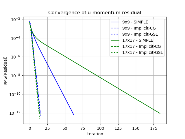
Figure 1: Comparison of SIMPLE and Implicit convergence histories for 9x9 and 17x17 meshes ($Re=100$).

Figure 1 demonstrates the benefits of an implicit solver over a segregated one for the test case discussed in Section 3. Convergence histories are shown for two meshes, 9x9 and 17x17, for the case with Reynolds number $Re=100$. The solid lines are from the SIMPLE solver and show the number of iterations being highly dependent on the mesh size. The pressure correction solver uses relaxation factors of 0.7 and 0.5 for the velocity and pressure respectively - these are close to the optimal values. The linearised pressure correction and momentum equations are solved to an error of less than $10^{-12}$ using a conjugate gradient (CG) solver. The dashed lines show the convergence of the implicit solver with both relaxation factors set to 1.0 and the linearised coupled equations also solved to $10^{-12}$ using a CG solver. The dotted lines show the classical eigen-solution [37] using the GNU scientific library (GSL) [31] to solve for the eigen-decomposition of the coupled matrix. In both cases, the implicit solver convergences far more rapidly and the convergence is independent of the mesh size. This is also the case for the 33x33 mesh (not shown) where SIMPLE requires 786 iterations and the implicit solver using CG requires 15 iterations.

Using GSL to solve the coupled matrix illustrates the time complexity of classical eigen-decomposition. For the 17x17 mesh, the full implicit solution using CG took 0.06s. whereas GSL took over 24min. Both were run on the same Intel^® Core^© i9 12900K 3.2GHz processor.

3 Test case

The lid driven cavity is one of the canonical test cases for CFD with the first published applications dating from the 1970s [38, 32] and with reference solutions provided by [39]. This case continues to be used as a basic validation case for viscous incompressible flow solvers on coarse meshes [40].

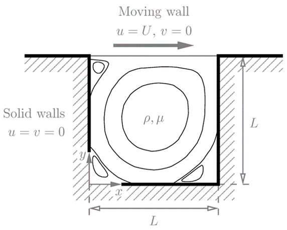
Figure 2: Overview of lid driven cavity test case, from [40].

Whilst, this work considers only low Reynolds number laminar flow, at higher Reynolds numbers this test case exhibits more complicated phenomena such as recirculations, turbulent flow structures and laminar to turbulent transition. Figure 2 from [40] gives an indication of some of the 2 dimensional flow structures. In 3D, the flow demonstrates complex unsteady turbulence phenomena such as inhomogeneous turbulence and small scale helical structures [41, 42]. [42] used a staggered mesh and a derivative of the SIMPLE scheme on a $64\times 64\times 64$ mesh. [43] used the equivalent of a $129\times 129\times 129$ mesh to perform direct numerical simulations of the turbulent flow in a 3D cavity. Calculations of this type are attractive for quantum computing as they explicitly resolve all the turbulence phenomena and do not require complicated and highly non-linear physical models of turbulence.

CFD mesh	matrix rank	#non-zeros	$|\lambda_{min}|$	$|\lambda_{max}|$	$\kappa$	HHL
5x5	76	265	$3.53\times 10^{-2}$	0.728	20.7	14 (7 + 6 + 1)
9x9	244	1,105	$5.72\times 10^{-3}$	0.415	72.6	18 (9 + 8 + 1)
17x17	868	4,513	$5.22\times 10^{-4}$	0.252	482	23 (11 + 11 + 1)
33x33	3,268	18,241	$3.59\times 10^{-5}$	0.137	3,806	27 (13 + 13 + 1)

Table 1: Dimensions, eigenvalue range and condition number for implicit $Re=100$ matrix. The HHL column gives an estimate of the number of logical qubits needed by HHL (state + eigenvalue + ancilla qubits).

Table 1 gives the characteristics of the implicit matrices for a range of mesh sizes. There are two factors of note: (a) the matrix ranks are not a power of 2; and, (b) the eigenvalues are calculated for the Hermitian matrix used by HHL and hence are real-valued. The eigenvalues occur in pairs of the same value with opposite signs. In order for the system to be amenable to HHL, the matrices are extended by a diagonal block in the bottom left corner of the matrix to give a rank equal to the next largest power of 2. This is illustrated in Figure 3 which shows the sparsity pattern for the 9x9 mesh with a diagonal extension to give a rank of 256. The added diagonal entries are all set according to the CFD mesh spacing to give terms with the same order as the other matrix elements.

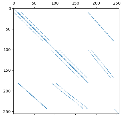
Figure 3: Sparsity pattern for 9x9 coupled system extended to have rank 256.

For the incompressible, laminar flows, as studied here, the only non-linear term is the fluid convection term. For the cases with a Reynolds number of 100, the convection term is only dominant very near to the moving lid. Hence, there are only minor variations in the eigenvalues of the linearised matrices. The rapid convergence of the implicit solver also ensures that after the first 2-3 iterations, variations in the eigenvalues are in the second or third significant figures. Section 5.3 considers higher Reynolds numbers where the effect of a greater initial variation in the eigenvalues is discussed.

Also of interest in Table 1 is that the condition numbers are significantly lower than for the pressure correction matrices reported by [13]. For example, the condition number for the pressure correction matrix on the 17x17 mesh is 3,500 compared to 482 for the implicit matrix. This means that whilst the rank of the implicit matrix is 4 times larger, the condition number is 8 times lower and the HHL emulations reduce by 1 qubit.

Unless otherwise stated, all calculations are for a Reynolds number of 100.

4 Hybrid CFD solver

Since the implicit matrices, $A$, listed in Table 1 are non-symmetric, they must be symmetrised to create a Hermitian operator for the Quantum Linear Equation Solver (QLES):

$$H=\begin{pmatrix}0&A\\ A^{\dagger}&0\end{pmatrix}$$ (4)

And the linear system to be solved becomes:

$$H\begin{pmatrix}0\\ x\end{pmatrix}=\begin{pmatrix}b\\ 0\end{pmatrix}$$ (5)

Matrix preparation for the HHL circuit requires the matrix $H$ to be decomposed into a linear combination of $M$ unitaries (LCU):

$$H=\sum_{i=1}^{M}\alpha_{i}U_{i}$$ (6)

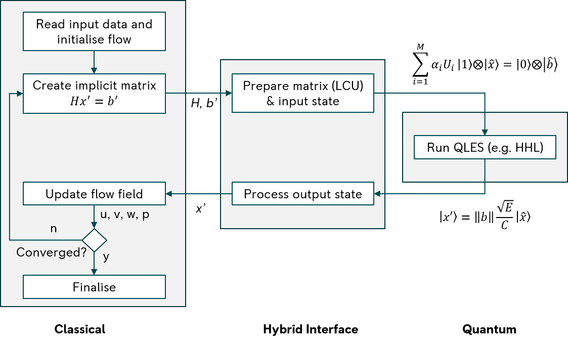
Figure 4: Hybrid implicit CFD solver. Hats denote normalised variables.

The LCU decomposition takes place on the classical computer and, as shown by [13], can become the dominant computational cost of a hybrid solver. Figure 4 gives an overview of the hybrid implicit CFD solver and shows the benefit of placing all the matrix inversions on a quantum device. In this work, the QLES is emulated on a classical computer using the circuit shown in Figure 5. The emulated HHL solver is as in [13] and is not repeated here.

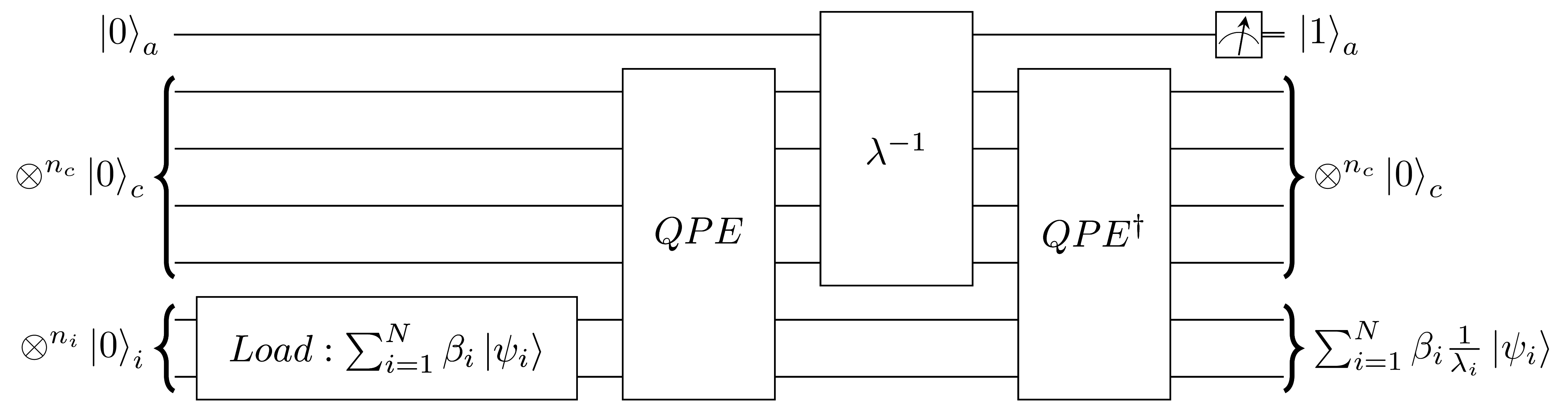
Figure 5: Outline of HHL circuit consisting of 3 registers: input register (i), clock register for eigenvalues (c), ancilla register (a).

It will be instructive later to refer to the linear algebra that underpins the HHL algorithm. Since H is Hermitian, all the eigenvalues are real and the eigenvectors form an orthonormal basis for the space of $N$-dimensional vectors. The right hand side vector can, therefore, be written as:

$$\ket{b}=\sum_{i=1}^{N}\beta_{i}\ket{\psi_{i}}$$ (7)

The coefficients $\beta_{i}$ are obtained from:

$$\beta_{i}=\bra{\psi_{i}}\ket{b}$$ (8)

The eigenvectors of $H$ are also the eigenvectors of $H^{-1}$ and the eigenvalues of $H^{-1}$ are the inverse of the eigenvalues of $H$. Hence:

$$H^{-1}=\sum_{i=1}^{N}\frac{1}{\lambda_{i}}\ket{\psi_{i}}\bra{\psi_{i}}$$ (9)

The solution vector $\ket{x}$ can be written as:

$$\begin{split}\ket{x}&=H^{-1}\ket{b}\\ &=\sum_{i=1}^{N}\frac{1}{\lambda_{i}}\ket{\psi_{i}}\bra{\psi_{i}}\sum_{j=1}^{N}\beta_{j}\ket{\psi_{j}}\\ &=\sum_{i=1}^{N}\beta_{i}\frac{1}{\lambda_{i}}\ket{\psi_{i}}\end{split}$$ (10)

If all the eigenvalues and vectors of $H$ can be found, then solving for $\ket{x}$ is straightforward. This has always been the case, but classical algorithms for computing all the eigen-pairs have computational complexity $\mathcal{O}(n^{3})$. By contrast, the HHL algorithm has complexity $\mathcal{O}(log(n)s^{2}\kappa^{2}/\epsilon)$ where $s$ is the maximum number of non zero entries per row or column; $\kappa$ is the condition number of the matrix; and $\epsilon$ is the precision. In this study, the matrices are small enough to classically compute their eigen-spectra.

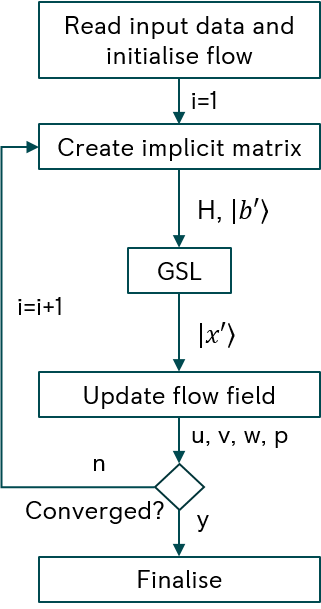
(a) Classical linear solver.

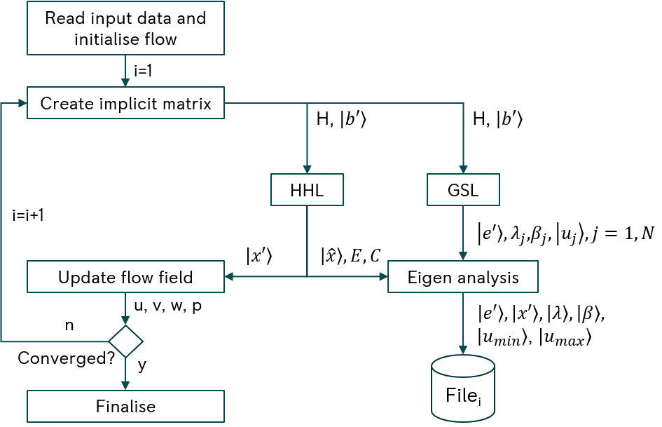
(b) (Verification of HHL linear solutions.

Figure 6: Modes of usage for GSL: (a) linear solver for reference fully classical solutions, (b) Verifier for each HHL solution using the same input state and matrices as HHL.

There are two modes of usage for GSL as shown in Figure 6. In the first mode, GSL is used as the linear solver for a completely classical solution. In the second mode, GSL is used to check the fidelity of the HHL solution for each outer iteration. GSL takes the same input vector and matrix as HHL and computes the classical solution for each linear system. The outer non-linear update uses the HHL solution and progresses exactly as if the GSL verifier were absent. For each iteration the following are written to an iteration stamped file: the GSL and HHL solutions; all the values of $\lambda$ and $\beta$; and, the eigenvectors corresponding to the minimum and maximum eigenvalues.

4.1 Interpreting the eigenvalues of a CFD matrix

Prior to presenting the results, it is useful to consider the physical interpretation of the eigen-system of a CFD matrix. Equation 3 effectively solves for corrections that eliminate errors in the satisfaction of the non-linear equations Equation 1. The eigenvectors correspond to error waves propagating in the flow.

The highest eigenvalues correspond to the most energetic errors and have eigenvectors with high frequency oscillations between neighbouring points in the CFD mesh. See the green line in Figure 16. Since the CFD discretisation directly connects neighbouring points, the errors lead to high residuals and are rapidly damped by the solver. In some discretisation schemes, there is a velocity-pressure decoupling that leads to a linearised matrix which has a null space [44]. The null space allows the so-called pressure checker-board mode to go undamped. The staggered meshes used in this study have been chosen because they do not have a null space.

The lowest eigenvalues correspond to eigenvectors with low frequency oscillations that often have a wavelength equal to the dimension of the solution domain. These are associated with errors in one region that affect distant regions via convection or diffusion. See the blue line in Figure 16. The rationale of the multi-grid method [21] is that low frequency errors on a fine mesh have progressively higher frequencies on the sequence of coarser meshes. This is why in multi-grid terminology the solver is often referred to as a smoother.

Whilst variational solvers and linear equation solvers both result in a low energy state in which the $L_{2}$ norm of the residual errors is low, the following results show the necessity of knowing and resolving the full eigenvalue range for HHL.

5 Results

All results were run on a desktop PC with an Intel^® Core^© i9 12900K 3.2GHz Alder Lake 16 core processor and 64GB of 3,200MHz DDR4 RAM. The calculations were parallelised using OpenMP directives [45]. All calculations were performed using double precision arithmetic including the CFD solver. Whilst the test case does not require this level of precision, it ensures that trends in the HHL solver are not masked by the precision of the input state or the matrix.

The main concern of the following analysis is the impact that some of the parameters in the linear matrix solver, such as the number of qubits used, have on the iterative convergence of the outer non-linear iterations. This is intimately linked with the accuracy of each inner linear solution but, as will be shown, there are iterative instabilities that are not apparent in an individual inner solution. The hybrid solutions are compared with exact solutions obtained using GSL [31] which allows a full eigen-spectrum analysis to be performed. The eigen-spectrum is obtained for the same symmetric matrix, $H$, as used by HHL, using symmetric bi-diagonalisation and the QR reduction method (see §8.3 of [37]). The computed eigenvalues are accurate to an absolute accuracy of $\epsilon||A||_{2}$, where $\epsilon$ is the machine precision.

5.1 Matrix decomposition

Table 2 gives the number of unitaries in the LCU decomposition for each CFD mesh. The Pauli string approach used by [13] produces a rapidly increasing number of unitaries to the point that the decomposition was not attempted for the 17x17 and 33x33 meshes The 13x13 mesh is included to show the rate at which the number of Pauli strings increases.

CFD mesh	#LCU unitaries
	Pauli strings	Simple 1-sparse	$\kappa$
5x5	4,132	634	20.7
9x9	16,104	2,234	72.6
13x13	48,956	5,050	205
17x17	-	9,338	482
33x33	-	38,138	3,806

Table 2: Number of unitaries in the LCU decomposition of the implicit CFD matrices.

For this work, an alternative simple 1-sparse decomposition is used where each pair of symmetric entries in $H$ corresponds to a pair of matrices in the LCU. The decomposition begins with 2 matrices $I_{+}=I$ and $I_{-}=-I$ where $I$ is the rank $N$ unit matrix. If $h_{ij}=h_{ji}$ are the symmetric entries in $H$, then, in both $I_{+}$ and $I_{-}$, the entries $ij$ and $ji$ are set to $1$ and the entries $ii$ and $jj$ are set the $0$. The coefficient for both matrices is $h_{ij}/2$. As Table 2 shows the number of unitaries is equal to the number of non-zero entries in $H$. Calculating this decomposition is extremely efficient and enables a broader range of emulations to be studied. However, the circuit implementation on a physical device has not been considered and is expected to be significant.

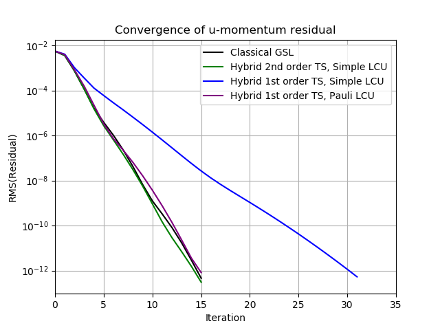
Figure 7: Effect of Trotter approximation on the convergence of the hybrid implicit solver on the 9x9 CFD mesh.

Figure 7 compares how the two LCU options affect the convergence rate on the 9x9 CFD mesh including the order of the Trotter-Suzuki (T-S) approximation [46, 47] for the Hamiltonian evolution operator. Both the Pauli string LCU with first order T-S and the simple pairwise LCU with second order T-S match the exact convergence rate very well. Whereas the simple pairwise LCU with first order T-S takes twice as many iterations to converge, despite having a factor of 8 fewer unitaries in the LCU.

The error orders for the Trotter-Suzuki approximations are given in Equations 11 to 12 where $\bar{\alpha}$ is an average LCU coefficient.

$$e^{-i\sum_{j=1}^{M}\alpha_{j}U_{j}t}=\left(\prod\limits_{j=1}^{M}e^{-i\alpha_{j}U_{j}t/r}\right)^{r}+\mathcal{O}(\bar{\alpha}^{2}t^{2}/r)$$ (11)

$$e^{-i\sum_{j=1}^{M}\alpha_{j}U_{j}t}=\left(\prod\limits_{j=1}^{M}e^{-i\alpha_{j}U_{j}t/2r}\prod\limits_{j=M}^{1}e^{-i\alpha_{j}U_{j}t/2r}\right)^{r}+\mathcal{O}(\bar{\alpha}^{3}t^{3}/r^{2})$$ (12)

For the Pauli string LCU, the root mean square of the LCU coefficients is $1.5\times 10^{-3}$, whereas, for the simple pairwise LCU it is $4.6\times 10^{-2}$. This leads to an almost 3 orders of magnitude difference in leading error term for the first order scheme which far outweighs the factor 8 increase in the number of unitaries.

An alternative to Trotter-Suzuki is qubitisation [48, 49, 50, 51, 52, 53] which provides an exact implementation of a unitary decomposition at the expense of an additional ancilla register for preparing the coefficients of the unitary decomposition. For the 9x9 mesh, the prepare register for the Pauli LCU would require 14 qubits and for the simple pairwise LCU would require 12 qubits. These are both more than the 8 qubits required by the HHL eigenvalue register (Table 3).

Unless otherwise stated, the following results used the second order Trotter-Suzuki formula with the simple pairwise LCU.

5.2 Precision

The analysis begins with the 9x9 CFD meshes as both the hybrid emulator and the exact GSL calculation can run the full implicit calculations in matters of minutes. Table 3 compares the exact eigenvalues with the range of values that can be resolved with different numbers of qubits in the eigenvalue register. A precision $(s,m,n)$ indicates $s$ sign qubits, $m$ integer qubits and $n$ fraction qubits. Where $m$ is negative, this indicates a right shift of the binary decimal point by $m$ spaces in the output bit patterns. The exact values are computed using GSL and taken from classical solutions after 10 non-linear iterations.

Precision	$\lambda_{min}$	$\lambda_{max}$	Total HHL qubits
Exact (GSL)	$\pm 0.00572$	$\pm 0.415$	-
(1,-1,6)	$\pm 0.01563$	$\pm 0.484$	16
(1,-1,7)	$\pm 0.00781$	$\pm 0.492$	17
(1,-1,8)	$\pm 0.00391$	$\pm 0.496$	18

Table 3: Exact eigenvalues and resolution for a range of precisions for the 9x9 implicit matrix.

Figure 8 compares the convergence of the $u$-momentum residuals for the 9x9 CFD mesh. Although the implicit solver solves a single coupled system, it is still instructive to analyse the individual equations as there can sometimes be iterative feedback mechanisms between the equations. This is not the case here and the $v$-momentum and continuity equations show similar convergence rates. The hybrid solution with 8 fraction qubits shows an almost identical convergence as the classical exact solution using GSL. This is as expected as the precision range is better than the exact eigenvalue range. The hybrid solution with 7 fraction qubits is marginally slower by 2 iterations. This is an indication that even a precision that is higher than the lowest eigenvalue by $37\%$ has an effect on convergence. The hybrid solution with 6 fraction qubits also converges but takes almost 5 times as many non-linear iterations. In this case, the precision is 2.7 times higher than the lowest eigenvalue.

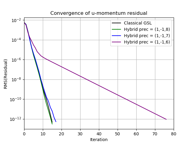
Figure 8: Effect of fraction precision on the convergence of the hybrid implicit solver on the 9x9 CFD mesh.

To further investigate the loss of precision, two measures of solution fidelity are used:

$$f_{n}=\bra{\hat{x}}\ket{\hat{e}}$$ (13)

$$f_{r}=\frac{\bra{x}\ket{e}}{\bra{e}\ket{e}}$$ (14)

$f_{n}$ is the normalised fidelity and compares the state vector at the end of HHL, $\ket{\hat{x}}$, with the normalised GSL solution, $\ket{\hat{e}}$. This is bounded by 0 and 1. $f_{r}$ is the raw fidelity and compares the dimensional solutions normalised by the exact state. This is not bounded by 0 and 1 but is equal to 1 if the two solution states match. $f_{n}$ and $f_{r}$ are evaluated for each non-linear iteration using GSL in verification mode as shown in Figure 6(b).

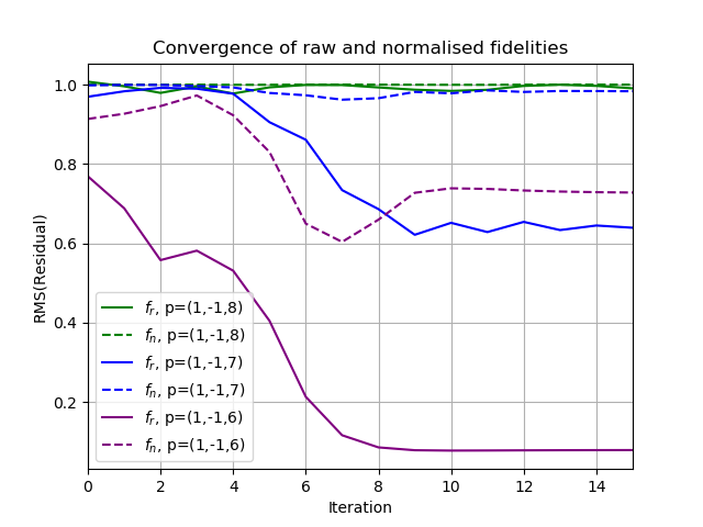
Figure 9: Comparison of fidelities $f_{n}$ and $f_{r}$ for the first 15 hybrid implicit iterations on the 9x9 CFD mesh.

Figure 9 compares these fidelities for the first 15 iterations of each precision. Even with (1,-1,8) precision, the raw fidelity shows a small amount of variation around 1.0, whilst the normalised fidelity is always above 0.99. With (1,-1,7) precision, although the normalised fidelity is close to 1.0, the raw fidelity starts dropping after 4 iterations and stabilises after 10 iterations at about 0.65. Even when the normalised fidelity is close to 1.0 after iteration 10, the raw fidelity remains at 0.65. The (1,-1,6) precision fidelities show the same behaviour as (1,-1,7) but more exaggerated with the raw fidelity dropping below 0.1 and not recovering.

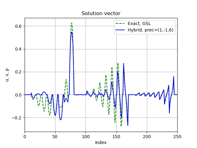
(a) Solutions for the 1st iteration.

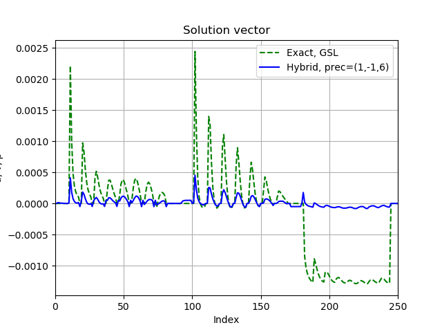
(b) Solutions for the 10th iteration.

Figure 10: Comparison of GSL and (1,-1,6) precision hybrid solutions after 1 and 10 non-linear iterations on the 9x9 CFD mesh. Graphs are for dimensionalised solutions which reduce as the non-linear iterations proceed.

The significant loss of fidelity in the (1,-1,6) solution between the first and tenth iterations is illustrated in Figure 10 which compares the hybrid and GSL verification solutions for these iterations. On the first iteration, there are clear differences between the GSL and hybrid solutions but the broad scale of the hybrid solution is generally correct. The solutions in the range [180, 243], which corresponds to the pressure field, match very well. At the tenth iteration, the amplitudes of the hybrid solution are much smaller than the GSL solution, particularly for the pressure field.

The fact that both solutions in Figure 10(b) use the same input vector and matrix, derived from the solution at iteration 9, suggests that the input vector is dominated by eigen coefficients that the HHL solution is unable to resolve in the preceding iterations. Using the GSL eigen decomposition, both solutions can be compared in terms of the coefficients in their eigen expansions using the equivalent of Equation 8.

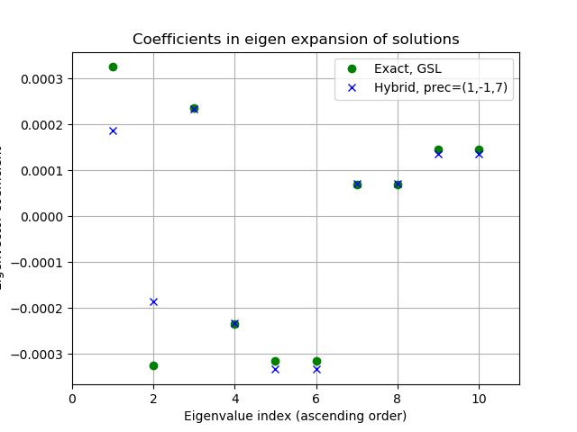
(a) (1,-1,7) precision, $6^{th}$ iteration.

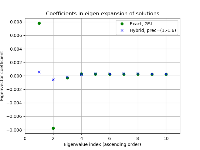
(b) (1,-1,6) precision, $10^{th}$ iteration.

Figure 11: Coefficients of the eigen-expansion of the GSL and hybrid solutions for the first 10 smallest eigenvalues.

Figure 11 compares for eigen coefficients for the first 10 smallest eigenvalues for the (1,-1,6) hybrid solution after 10 outer iterations and the (1,-1,7) hybrid solution after 6 outer iterations. These solutions were chosen as, they have approximately the same level of residual convergence. The fist four eigenvalues are below the $\pm 0.015625$ precision of 6 fraction qubits and only the first two are below the $\pm 0.0078125$ precision of 7 fraction qubits. Note that these comparisons are between two different precision calculations at roughly the same level of convergence.

Considering Figure 11(a), the coefficients for the (1,-1,7) solution match, the exact GSL coefficients very well even for the first eigenvalue pair that it has not resolved. From Figure 11(b), the coefficients for the (1,-1,6) solution fail to match the exact coefficients for the first eigenvalue pair by an order of magnitude. Since this is largest coefficient in the eigen-expansion, it explains why the raw fidelity is so low.

These results are indicative of an iterative feed-forward mechanism at play. The failure to resolve the lowest eigenvalues creates a constructive reinforcement on consecutive non-linear iterations whereby the residuals corresponding to unresolved eigenvalues are under corrected. Hence, $\beta_{0}$ and $\beta_{1}$ in Equation 7 increase for successive input vectors, as do the coefficients of the exact solution $\beta_{0}/\lambda_{0}$ and $\beta_{1}/\lambda_{1}$. The disparity increases for about 8 iterations until an equilibrium is reached and the hybrid solution slowly converges as shown in Figure 8. The (1,-1,7) solution is subject to the same mechanism but this has a much more marginal effect.

Since the eigen-expansions of both the HHL and GSL solutions are available, the effect of the discrepancy in the first two eigen coefficients can be used to create a corrected HHL solution as shown in Equation 15.

$$\begin{split}\ket{x}_{hhl}&=\sum_{i=1}^{n}\beta_{x,i}\ket{\psi_{i}}\bra{\psi_{i}}\\ \ket{x}_{cor}&=\sum_{i=1}^{n}\beta_{x,i}\ket{\psi_{i}}\bra{\psi_{i}}+\left(\frac{\beta_{1}}{\lambda_{1}}-\beta_{x,1}\right)\ket{\psi_{1}}+\left(\frac{\beta_{2}}{\lambda_{2}}-\beta_{x,2}\right)\ket{\psi_{2}}\end{split}$$ (15)

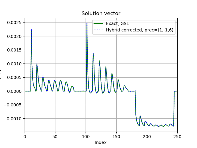
Figure 12: Comparison of corrected HHL solution from Figure 10(b) using Equation 15 and exact GSL solution.

Figure 12 compares the corrected HHL and GSL solutions after iteration 10 using a precision of (1,-1,6) for HHL. Whilst there are some tiny discrepancies, the agreement is far better than expected. On a positive note, this illustrates that HHL has accurately represented all the eigen coefficients that it is able to resolve. On the negative side, the failure to resolve the lowest eigenvalues has iteratively driven the calculation to a state where the residual errors, $\ket{b}$, are dominated by the eigenvectors corresponding to the unresolved eigenvalues.

5.2.1 Resolving the lowest eigenvalue

The above analysis shows that a good estimation of the lowest eigenvalue is essential for HHL to be used within an outer non-linear iterative solver. Even an error of less than a factor of 2 is sufficient to degrade the rate of non-linear convergence. However, if HHL were able to deliver an exponential speed-up, a linear degradation in the outer rate of convergence would not remove the quantum advantage. There are a number of challenges to obtaining exponential speed-up with HHL. Not least, the depth of the eigenvalue inversion circuit. Figure 13 shows all 512 $\beta$ coefficients in the eigen-expansion of the output vector on the 9x9 mesh after 6 iterations. Also shown is a line corresponding the $L_{2}$ norm of the input vector. Well over half of the coefficients are within an order of magnitude of the $L_{2}$ norm and, possibly, the majority are needed to get an accurate solution. A logarithmic depth circuit would contain 9 rotations and, hence, would accurately resolve only 9 of the 512 eigen-coefficients.

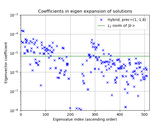
Figure 13: Coefficients, $\beta$, of the eigen-expansion of the (1,-1,8) solution on the 9x9 CFD mesh after 6 iterations. Green line shows the $L_{2}$ norm of $\ket{b}$.

Assuming an efficient eigenvalue inversion circuit is available, the estimation of lowest eigenvalue is an input to the circuit design and, currently, must be calculated classically. The power method (see §7.3.1 of [37]) provides a way to estimate the maximum eigenvalue using only matrix-vector multiplication. The power method can be applied to the inverse of the matrix, $H^{-1}$ to find the minimum eigenvalue. However, inverting $H$ is equivalent to solving the linear system. Whilst this is potentially a one-off initial calculation, or one that is only repeated a small number of times, it is classically intractable for the size of matrices at which quantum advantage might be expected.

5.2.2 Resolving the largest eigenvalue

The 17x17 coupled matrix has a maximum eigenvalue of 0.2519 which is very close to a binary precision of $\frac{1}{4}$ and, hence, suitable for examining its resolution. Table 4 shows the precision ranges for (1,-1,11) and (1,-2,11). Both fully resolve the lowest eigenvalue and the (1,-2,11) precision is within $1\%$ of the largest eigenvalue.

Precision	$\lambda_{min}$	$\lambda_{max}$	Total HHL qubits
Exact (GSL)	$\pm 0.000522$	$\pm 0.2519$	-
(1,-1,11)	$\pm 0.000488$	$\pm 0.4995$	23
(1,-2,11)	$\pm 0.000488$	$\pm 0.2495$	22

Table 4: Exact eigenvalues and resolution for a range of precisions for the 17x17 implicit matrix.

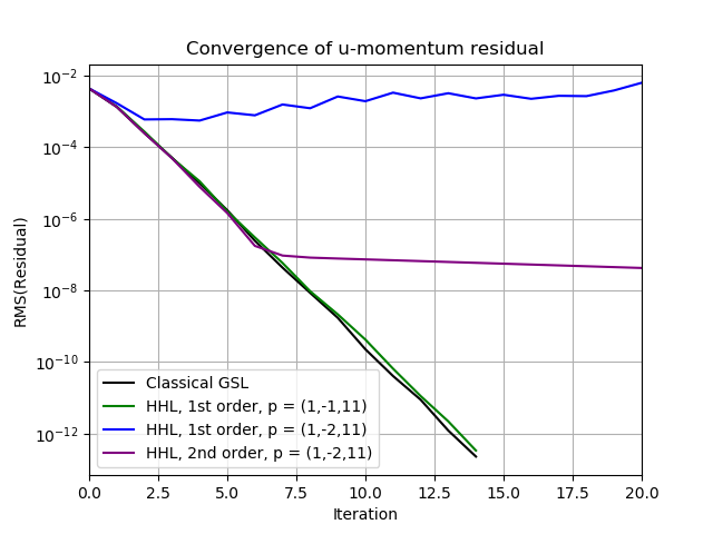
(a) Convergence histories.

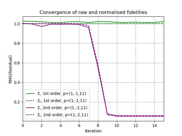
(b) (Raw and normalised fidelities.

Figure 14: Effect of precision and Trotter-Suzuki order for 17x17 CFD mesh.

Figure 14(a) compares the GSL convergence histories with the hybrid HHL solutions for both precisions and for different Trotterisation orders. The (1,-1,11) emulation spans the full range of eigenvalues and matches the exact GSL convergence with the first order Trotter scheme. However, changing the integer precision has a secondary effect, that does not happen with the fraction precision, which is it to change the evolution time in the quantum phase estimation (QPE) step. In these emulations, the time-step must be consistent with bit resolution of the eigenvalue register and is set as:

$$t=\frac{2\pi}{2^{s+i}}$$ (16)

where, as before, $s$ is the number of sign qubits and $i$ is the number of fraction qubits. Hence, reducing the integer precision by one qubit doubles the QPE evolution time.

In both the first and second order simulations the exponent is $r=5$ and the mean LCU coefficient is approximately $\bar{\alpha}=0.02$. For the (1,-2,11) precision, the evolution time step is $4\pi$. From Equations 11 to 12 this gives a leading error of order $10^{-2}$ for the first order scheme and $10^{-4}$ for the 2nd order scheme.

The failure to converge of the first order (1,-2,11) solution in Figure 14(a) is due to the Trotter approximation and not the loss of precision. The second order solution initially converges almost identically to the exact solution, reducing the residual by almost 5 orders of magnitude, before stagnating from iteration 6 onward. The 2nd order fidelities in Figure 14(b) show a different character from those for the minimum eigenvalue, with both the raw and normalised fidelities moving in concert.

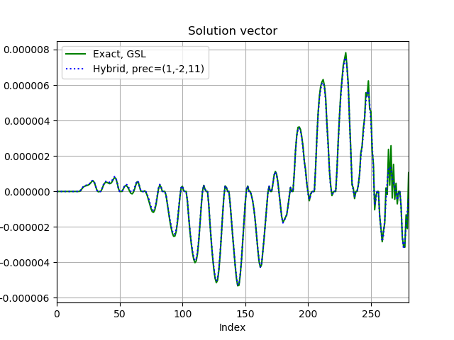
(a) Iteration 8.

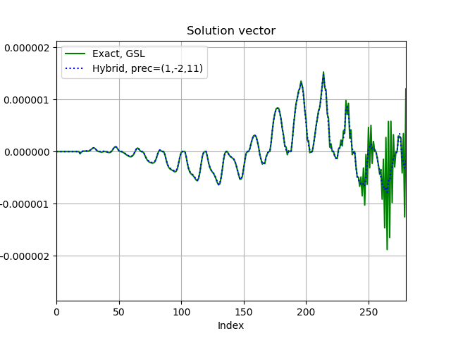
(b) (Iteration 9.

Figure 15: Solutions for the u-momentum equation at iterations 8 and 9 for 17x17 CFD mesh.

Figure 15 shows the solutions for the u-momentum part of the state vector after iterations 8 and 9. Small high frequency oscillations near index 255 at iteration 8, grow rapidly at iteration 9 and by iteration 10 (not shown) dominate the solution. There are no oscillations present at iteration 6 and only very minor oscillations at iteration 7. Note also that the oscillations are in the GSL verification solution and not the hybrid solution. These have built up in the input vector as before.

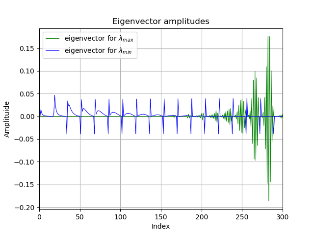
Figure 16: Amplitudes [0,300] of the eigenvectors for the minimum and maximum eigenvalues on the 17x17 CFD mesh.

Figure 16 compares the first 300 amplitudes of the eigenvectors for the minimum and maximum eigenvalues. The patterns largely repeat for the remaining amplitudes. As can be seen, the eigenvector for the largest eigenvalue corresponds to a high frequency oscillation between neighbouring grid points. As described in Section 4.1, mesh based CFD algorithms are designed to eliminate, or smooth, such oscillations very quickly. By failing to resolve the largest eigenvalue, the highest frequency eigenvector is not resolved and the oscillations that it would eliminate are allowed to persist. The character of a sudden switch at between iterations 7 and 9 is due to the small 1% difference between the eigenvalue and the precision. The oscillations begin on the first outer iteration at a level of $10^{-12}$ and grow until they reach $10^{-7}$ at which point they dominate the input and output vectors. If the precision difference were larger, then a more immediate effect would be expected.

As described in Section 4.1, the minimum eigenvalue corresponds to the eigenvector for the lowest frequency oscillations which CFD algorithms take many iterations to eliminate and why acceleration schemes such as multi-grid are successful. The spikes in the eigenvector amplitudes correspond to discontinuities where the mesh index flips from one side wall of the cavity to the other.

5.3 Reynolds number

The dimensions of the CFD mesh are not the only factors that influence the eigen-spectrum of the implicit matrix. The other important factor is Reynolds number defined by:

$$Re=\frac{\rho uL}{\mu}$$ (17)

Where $L$ is a representative length scale. For the cavity, $L$ is the cavity width, $u$ is the velocity of the lid, the density $\rho$ is unity and the viscosity $\mu$ is set to give the required value of $Re$.

Reynolds number	$\lambda_{min}$	$\lambda_{max}$	$\kappa$	HHL precision
100	$\pm 5.72\times 10^{-3}$	$\pm 0.415$	72.6	(1,-1,8)
1,000	$\pm 2.11\times 10^{-3}$	$\pm 0.363$	172	(1,-1,9)
10,000	$\pm 5.10\times 10^{-4}$	$\pm 0.352$	691	(1,-1,11)

Table 5: Exact eigenvalues and resolution for a range of precisions for the 9x9 implicit matrix after 10 non-linear iterations.

Table 5 gives the eigenvalues and qubit counts for Re=100, 1,000 and 10,000 for the 9x9 CFD mesh. A Reynolds number of 10,000 is the point at which the flow is expected to transition to turbulence. Each precision fully spans the corresponding eigenvalue range.

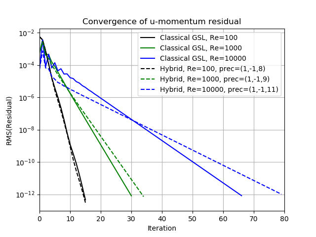
Figure 17: Effect of Reynolds number on the convergence of the hybrid implicit solver on the 9x9 CFD mesh.

Figure 17 compares the GSL and hybrid convergence histories for the three Reynolds numbers. There is a shared trend for the number of non-linear iterations to increase with Reynolds number. This is because the higher the Reynolds number, the higher the non-linear inertial effects are in the fluid. The solution of the linearised inner equations is then a less good approximation to the final non-linear solution.

There is also a trend that the hybrid solver takes an increasing number of additional iterations relative to GSL as the Reynolds number increases. This was traced to the initial iterations for the Re 1,000 and 10,000 having lower minimum eigenvalues than expected. The numbers in Table 5 are taken from the GSL solutions after 10 iterations. For the Re=1,000 case this gave a low raw fidelity of 0.67 for the first iteration. For the Re=10,000 case, the raw fidelities ranged from 0.23 to 0.66 for the first 3 iterations. After that, both cases consistently had raw fidelities close to 1. As shown previously, unresolved solution components in the output state can transfer to the next input state and slow convergence. This was confirmed by running the Re=1,000 case with an additional 2 fraction qubits. The raw fidelities were above 0.98 for all iterations and the hybrid solver took just 1 more iteration that the GSL solution.

6 Conclusions

Quantum algorithms for direct matrix inversion, such as HHL and QSVT, mean that quantum CFD algorithms should not need to follow the same path as classical solvers towards highly sophisticated iterative solvers such as those based on Krylov sub-spaces. Coupled with implicit discretisation schemes, these provide a promising route to Quantum Advantage, albeit on Fault Tolerant devices.

This work has demonstrated the importance of assessing HHL within the context of an outer non-linear iteration rather than simply as linear solver of a individual matrix equation. The precision with which HHL resolves both the minimum and maximum eigenvalues has been shown to be crucial to how it behaves within a non-linear CFD solver. The behaviour has been shown to be consistent with how the eigenvalues and eigenvectors relate to the CFD discretisation. These findings are relevant to early Fault Tolerant CFD prototypes where every (logical) qubit is likely to count.

The importance of accurately estimating the eigenvalue range, particularly the maximum eigenvalue, has been illustrated. This is part of the classical computing overhead for hybrid algorithms discussed by [13] for the pressure correction equation. The matrix decomposition overhead using Pauli strings is more severe for the implicit method with the 9x9 CFD matrix decomposition containing 50 times more unitaries than the pressure correction matrix. A simple alternative has been used here, but this is unlikely to lead to efficient circuits. Although QSVT matrix inversion has not been studied, the observations on eigenvalue accuracy (i.e. condition number) and the high Pauli string count in the LCU are expected to be relevant to QSVT based CFD algorithms.

7 Acknowledgements

The permission of Rolls-Royce to publish this paper is gratefully acknowledged. The results were completed as part of funding received under the UK’s Commercialising Quantum Technologies Programme (Grant reference 10004857). This work has benefited from several technical discussions and the author would like to thank Neil Gillespie, Joan Camps and Christoph Sunderhauf of Riverlane; Jarrett Smalley of Rolls-Royce; and, Philippa Rubin of the STFC Hartree Centre.

References

- [1] M. Walport, M. Calder, C. Craig, D. Culley, R. de Cani, C. Donnelly, R. Douglas, B. Edmonds, J. Gascoigne, N. Gilbert, et al., Computational Modelling: Technological Futures. Government Office for Science, 2018.
- [2] P. Givi, A. J. Daley, D. Mavriplis, and M. Malik, “Quantum speedup for aeroscience and engineering,” AIAA Journal, vol. 58, no. 8, pp. 3715–3727, 2020.
- [3] R. Steijl, “Quantum algorithms for fluid simulations,” Advances in Quantum Communication and Information, p. 31, 2019.
- [4] B. Kacewicz, “Almost optimal solution of initial-value problems by randomized and quantum algorithms,” Journal of Complexity, vol. 22, no. 5, pp. 676–690, 2006.
- [5] P. C. Costa, S. Jordan, and A. Ostrander, “Quantum algorithm for simulating the wave equation,” Physical Review A, vol. 99, no. 1, p. 012323, 2019.
- [6] F. Gaitan, “Finding flows of a navier–stokes fluid through quantum computing,” npj Quantum Information, vol. 6, no. 1, pp. 1–6, 2020.
- [7] A. Suau, G. Staffelbach, and H. Calandra, “Practical quantum computing: solving the wave equation using a quantum approach,” ACM Transactions on Quantum Computing, vol. 2, no. 1, pp. 1–35, 2021.
- [8] B. Ljubomir, “Quantum algorithm for the navier–stokes equations by using the streamfunction-vorticity formulation and the lattice boltzmann method,” International Journal of Quantum Information, p. 2150039, 2022.
- [9] C. Lu, Z. Hu, B. Xie, and N. Zhang, “Quantum cfd simulations for heat transfer applications,” in ASME International Mechanical Engineering Congress and Exposition, vol. 84584, p. V010T10A050, American Society of Mechanical Engineers, 2020.
- [10] M. Lubasch, J. Joo, P. Moinier, M. Kiffner, and D. Jaksch, “Variational quantum algorithms for nonlinear problems,” Physical Review A, vol. 101, no. 1, p. 010301, 2020.
- [11] O. Kyriienko, A. E. Paine, and V. E. Elfving, “Solving nonlinear differential equations with differentiable quantum circuits,” Physical Review A, vol. 103, no. 5, p. 052416, 2021.
- [12] A. C. Vazquez, R. Hiptmair, and S. Woerner, “Enhancing the quantum linear systems algorithm using richardson extrapolation,” arXiv preprint arXiv:2009.04484, 2020.
- [13] L. Lapworth, “A hybrid quantum-classical cfd methodology with benchmark hhl solutions,” arXiv preprint arXiv:2206.00419, 2022.
- [14] S. Patankar and D. Spalding, “A calculation procedure for heat, mass and momentum transfer in three-dimensional parabolic flows,” Int. J. Heat Mass Transfer, vol. 15, pp. 1787–1806, 1972.
- [15] D. Ammour and G. J. Page, “The subgrid-scale approach for modeling impingement cooling flow in the combustor pedestal tile,” Journal of Heat Transfer, vol. 140, no. 4, 2018.
- [16] A. W. Harrow, A. Hassidim, and S. Lloyd, “Quantum algorithm for linear systems of equations,” Physical review letters, vol. 103, no. 15, p. 150502, 2009.
- [17] C. Misev, Development and Optimisation of an Implicit CFD Solver in Hydra. University of Surrey (United Kingdom), 2018.
- [18] L. Lapworth, “Hydra-cfd: a framework for collaborative cfd development,” in International conference on scientific and engineering computation (IC-SEC), vol. 30, 2004.
- [19] D. Amirante, P. Adami, and N. J. Hills, “A multifidelity aero-thermal design approach for secondary air systems,” Journal of Engineering for Gas Turbines and Power, vol. 143, no. 3, 2021.
- [20] P. Moinier, J.-D. Muller, and M. B. Giles, “Edge-based multigrid and preconditioning for hybrid grids,” AIAA journal, vol. 40, no. 10, pp. 1954–1960, 2002.
- [21] P. Wesseling, “A robust and efficient multigrid method,” in Multigrid Methods, pp. 614–630, Springer, 1982.
- [22] M. R. Hestenes and E. Stiefel, “Methods of conjugate gradients for solving,” Journal of research of the National Bureau of Standards, vol. 49, no. 6, p. 409, 1952.
- [23] R. Fletcher, “Conjugate gradient methods for indefinite systems,” in Numerical analysis, pp. 73–89, Springer, 1976.
- [24] H. A. Van der Vorst, “Bi-cgstab: A fast and smoothly converging variant of bi-cg for the solution of nonsymmetric linear systems,” SIAM Journal on scientific and Statistical Computing, vol. 13, no. 2, pp. 631–644, 1992.
- [25] Y. Idomura, T. Ina, S. Yamashita, N. Onodera, S. Yamada, and T. Imamura, “Communication avoiding multigrid preconditioned conjugate gradient method for extreme scale multiphase cfd simulations,” in 2018 IEEE/ACM 9th Workshop on Latest Advances in Scalable Algorithms for Large-Scale Systems (scalA), pp. 17–24, IEEE, 2018.
- [26] Y. Saad and M. H. Schultz, “Gmres: A generalized minimal residual algorithm for solving nonsymmetric linear systems,” SIAM Journal on scientific and statistical computing, vol. 7, no. 3, pp. 856–869, 1986.
- [27] S. Balay, W. Gropp, L. C. McInnes, and B. F. Smith, “Petsc, the portable, extensible toolkit for scientific computation,” Argonne National Laboratory, vol. 2, no. 17, 1998.
- [28] J. M. Martyn, Z. M. Rossi, A. K. Tan, and I. L. Chuang, “Grand unification of quantum algorithms,” PRX Quantum, vol. 2, no. 4, p. 040203, 2021.
- [29] A. Gilyén, Y. Su, G. H. Low, and N. Wiebe, “Quantum singular value transformation and beyond: exponential improvements for quantum matrix arithmetics,” in Proceedings of the 51st Annual ACM SIGACT Symposium on Theory of Computing, pp. 193–204, 2019.
- [30] Y. Dong, X. Meng, K. B. Whaley, and L. Lin, “Efficient phase-factor evaluation in quantum signal processing,” Physical Review A, vol. 103, no. 4, p. 042419, 2021.
- [31] B. Gough, GNU scientific library reference manual. Network Theory Ltd., 2009.
- [32] K. Ghia, W. Hankey, JR, and J. Hodge, “Study of incompressible navier-stokes equations in primitive variables using implicit numerical technique,” in 3rd Computational Fluid Dynamics Conference, p. 648, 1977.
- [33] H. K. Versteeg and W. Malalasekera, An introduction to computational fluid dynamics: the finite volume method. Pearson education, 2007.
- [34] Z. Mazhar, “A novel fully implicit block coupled solution strategy for the ultimate treatment of the velocity–pressure coupling problem in incompressible fluid flow,” Numerical Heat Transfer, Part B: Fundamentals, vol. 69, no. 2, pp. 130–149, 2016.
- [35] A. Puyero, D. Zingg, A. Puyero, and D. Zingg, “An efficient newton-gmres solver for aerodynamic computations,” in 13th Computational Fluid Dynamics Conference, p. 1955, 1997.
- [36] B. Blais, L. Barbeau, V. Bibeau, S. Gauvin, T. El Geitani, S. Golshan, R. Kamble, G. Mirakhori, and J. Chaouki, “Lethe: An open-source parallel high-order adaptative cfd solver for incompressible flows,” SoftwareX, vol. 12, p. 100579, 2020.
- [37] G. H. Golub and C. F. Van Loan, Matrix computations. JHU press, 2013.
- [38] R. E. Smith Jr and A. Kidd, “Comparative study of two numerical techniques for the solution of viscous flow in a driven cavity,” NASA Special Publication, vol. 378, p. 61, 1975.
- [39] U. Ghia, K. N. Ghia, and C. Shin, “High-re solutions for incompressible flow using the navier-stokes equations and a multigrid method,” Journal of computational physics, vol. 48, no. 3, pp. 387–411, 1982.
- [40] H. Redal, J. Carpio, P. A. García-Salaberri, and M. Vera, “Dynamfluid: Development and validation of a new gui-based cfd tool for the analysis of incompressible non-isothermal flows,” Processes, vol. 7, no. 11, p. 777, 2019.
- [41] R. Bouffanais, M. O. Deville, and E. Leriche, “Large-eddy simulation of the flow in a lid-driven cubical cavity,” Physics of Fluids, vol. 19, no. 5, p. 055108, 2007.
- [42] D. A. Shetty, T. C. Fisher, A. R. Chunekar, and S. H. Frankel, “High-order incompressible large-eddy simulation of fully inhomogeneous turbulent flows,” Journal of computational physics, vol. 229, no. 23, pp. 8802–8822, 2010.
- [43] G. Courbebaisse, R. Bouffanais, L. Navarro, E. Leriche, and M. Deville, “Time-scale joint representation of dns and les numerical data,” Computers & fluids, vol. 43, no. 1, pp. 38–45, 2011.
- [44] F.-S. Lien, “A pressure-based unstructured grid method for all-speed flows,” International journal for numerical methods in fluids, vol. 33, no. 3, pp. 355–374, 2000.
- [45] R. Chandra, L. Dagum, D. Kohr, R. Menon, D. Maydan, and J. McDonald, Parallel programming in OpenMP. Morgan kaufmann, 2001.
- [46] H. F. Trotter, “On the product of semi-groups of operators,” Proceedings of the American Mathematical Society, vol. 10, no. 4, pp. 545–551, 1959.
- [47] M. Suzuki, “Improved trotter-like formula,” Physics Letters A, vol. 180, no. 3, pp. 232–234, 1993.
- [48] G. H. Low and I. L. Chuang, “Hamiltonian Simulation by Qubitization,” Quantum, vol. 3, p. 163, July 2019.
- [49] A. M. Childs and N. Wiebe, “Hamiltonian simulation using linear combinations of unitary operations,” arXiv preprint arXiv:1202.5822, 2012.
- [50] R. Kothari, Efficient algorithms in quantum query complexity. PhD thesis, University of Waterloo, 2014.
- [51] D. W. Berry, A. M. Childs, R. Cleve, R. Kothari, and R. D. Somma, “Simulating hamiltonian dynamics with a truncated taylor series,” Physical review letters, vol. 114, no. 9, p. 090502, 2015.
- [52] D. W. Berry, M. Kieferová, A. Scherer, Y. R. Sanders, G. H. Low, N. Wiebe, C. Gidney, and R. Babbush, “Improved techniques for preparing eigenstates of fermionic hamiltonians,” npj Quantum Information, vol. 4, no. 1, pp. 1–7, 2018.
- [53] R. Babbush, C. Gidney, D. W. Berry, N. Wiebe, J. McClean, A. Paler, A. Fowler, and H. Neven, “Encoding electronic spectra in quantum circuits with linear t complexity,” Physical Review X, vol. 8, no. 4, p. 041015, 2018.