Resolved SPLASH Chemodynamics in Andromeda’s PHAT Stellar Halo and Disk: On the Nature of the Inner Halo Along the Major Axis

Abstract

Stellar kinematics and metallicity are key to exploring formation scenarios for galactic disks and halos. In this work, we characterized the relationship between kinematics and photometric metallicity along the line-of-sight to M31’s disk. We combined optical HST/ACS photometry from the Panchromatic Hubble Andromeda Treasury (PHAT) survey with Keck/DEIMOS spectra from the Spectroscopic and Photometric Landscape of Andromeda’s Stellar Halo (SPLASH) survey. The resulting sample of 3512 individual red giant branch stars spans 4–19 projected kpc, making it a useful probe of both the disk and inner halo. We separated these stars into disk and halo populations by modeling the line-of-sight velocity distributions as a function of position across the disk region, where $\sim$73% stars have a high likelihood of belonging to the disk and $\sim$14% to the halo. Although stellar halos are typically thought to be metal-poor, the kinematically identified halo contains a significant population of stars ($\sim$29%) with disk-like metallicity ([Fe/H]_phot $\sim$ $-0.10$). This metal-rich halo population lags the gaseous disk to a similar extent as the rest of the halo, indicating that it does not correspond to a canonical thick disk. Its properties are inconsistent with those of tidal debris originating from the Giant Stellar Stream merger event. Moreover, the halo is chemically distinct from the phase-mixed component previously identified along the minor axis (i.e., away from the disk), implying contributions from different formation channels. These metal-rich halo stars provide direct chemodynamical evidence in favor of the previously suggested “kicked-up” disk population in M31’s inner stellar halo.

1 Introduction

The formation and evolution of stellar disks is a significant part of the mass assembly history of galaxies. In the local universe, disk galaxies have been observed to possess dynamically hot “thick” disk components in their vertical structure (e.g., Chiba & Beers 2000; Yoachim & Dalcanton 2006; but see also Bovy et al. 2012). Multiple physical mechanisms have been proposed to explain the formation of thick disks, including early in-situ star formation within a turbulent gaseous disk (Bournaud et al., 2009; Forbes et al., 2012) and heating of an initially thin stellar disk by internal perturbations (e.g., Sellwood & Carlberg 1984; Jenkins & Binney 1990; Lacey 1984; Schönrich & Binney 2009a, b; Loebman et al. 2011). However, the hierarchical assembly process may also provide channels for thick disk formation via the accretion of gas (e.g., Brook et al. 2004) and ex-situ stellar material (Abadi et al., 2003) deposited at large scale heights or heating driven by satellite impacts (Quinn et al., 1993; Velazquez & White, 1999; Hopkins et al., 2008; Kazantzidis et al., 2008; Villalobos & Helmi, 2008; Purcell et al., 2009). The formation of the dynamically hot thick disk may therefore be inextricably connected to the inner stellar halo by merger history.

M31’s proximity (785 kpc) and inclination (77^∘) result in an unrivaled opportunity to study galaxy disks beyond the Milky Way (MW). Resolved stellar spectroscopy along the line-of-sight to M31’s disk has transformed our understanding of the galaxy’s inner structure. Based on spectra of over 5000 red giant branch (RGB) stars, Dorman et al. (2012) discovered a rotating spheroid ($\sigma_{v}$ $\sim$ 140 km s^-1) that exceeded $\sim$10% of the total stellar population in a region dominated by the disk in UV/optical images ($R_{\rm proj}$ $\sim$ 4–20 kpc). However, surface-brightness decompositions indicated that the bulge should not contribute to stellar populations outside of M31’s inner few kiloparsecs (Courteau et al., 2011; Gilbert et al., 2012; Williams et al., 2012). The structural decomposition of Dorman et al. (2013), which simultaneously accounted for surface brightness profiles, the luminosity function, and kinematics, demonstrated that the spheroid corresponded to a stellar halo. Dorman et al. (2013) also found evidence for an excess of stars with a disk-like luminosity function compared to dynamically-based expectations for the disk contribution. These stars could have been born in the disk, but kinematically heated into the stellar halo.

Further studies imply a possible merger origin for the connection between the formation of the halo and disk. Dorman et al. (2015) revealed a steep relationship between age and velocity dispersion in M31’s disk region ($\sigma_{v}$ $\sim$ 90 km s^-1 for 4 Gyr ages), concluding that this could be explained by a combination of continuous but non-uniform heating of the disk by mergers. Quirk et al. (2019) identified a trend of monotonically increasing asymmetric drift with stellar age that was consistent with a 4:1 merger event occurring within the last 4 Gyr (Quirk & Patel, 2020). Moreover, a recent major merger (as explored by Hammer et al. 2018; D’Souza & Bell 2018) could simultaneously explain M31’s 2–4 Gyr old global burst of star formation (Bernard et al., 2015; Williams et al., 2015), its chemically homogeneous extended disk (15–40 kpc; Ibata et al. 2005), and thickened disk structure and kinematics (Dorman et al. 2012, 2015; Dalcanton et al. 2015; but see also Collins et al. 2011). Studies of planetary nebulae in M31’s disk have similarly concluded that its age-dispersion relation could result from a major merger (Bhattacharya et al., 2019).

Despite the wealth of kinematical information, comprehensive chemodynamical investigations are lacking across M31’s disk region. Prior studies of resolved stellar populations have been largely restricted to either chemical analyses informed by photometry (e.g., Gregersen et al. 2015; Telford et al. 2019) or focused on dynamics (e.g., Dorman et al. 2012, 2013, 2015; Quirk et al. 2019). In order to circumvent crowding, previous chemodynamical efforts have been limited to the outer disk ($\gtrsim$ 15 kpc) in the northeast (Ibata et al., 2005) and the southwest (Collins et al., 2011). To date, chemical abundances ([Fe/H] and [$\alpha$/Fe]) for individual stars have been measured for only a small sample of stars in M31’s outer disk (at 26 projected kpc; Escala et al. 2020a). Recently, oxygen and argon abundances from emission lines in planetary nebulae have provided an additional method to probe the chemical evolutionary history of M31’s inner disk (Bhattacharya et al., 2022; Arnaboldi et al., 2022).

In this work, we combine resolved spectroscopy from the Spectroscopic and Photometric Landscape of Andromeda’s Stellar Halo (SPLASH; Guhathakurta et al. 2005; Gilbert et al. 2006) survey and photometry from the Panchromatic Hubble Andromeda Treasury (PHAT; Dalcanton et al. 2012; Williams et al. 2014) to perform the first large-scale stellar chemodynamical analysis of M31’s inner disk region ($\lesssim$ 15 kpc) in an effort to explore disk-halo formation scenarios. This approach enables us to disentangle the inner stellar halo from the disk as well as identify chemically distinct stellar populations. In Section 2, we introduce the photometric and spectroscopic data sets used in this work. We evaluate M31 membership and perform a kinematical decomposition of the disk region in Section 3. We correct for dust effects and describe photometric metallicity measurements for RGB stars in Section 4. Section 5 investigates the chemical and dynamical properties of the disk and halo, whereas Section 6 places these results in the context of the literature on M31, the MW, and disk galaxy formation in general. We summarize our main findings in Section 7.

2 Data

2.1 PHAT Photometry

We used stellar catalogs based on Hubble Space Telescope (HST) Wide Field Camera 3 (WFC3) and Advanced Camera for Surveys (ACS) images from the PHAT survey (Dalcanton et al., 2012; Williams et al., 2014)). PHAT produced six-filter UV (F275W, F336W), optical (F475W, F814W), and IR (F110W, F160W) photometry across the northeastern disk of M31 out to 20 projected kpc from M31’s center for 117 million stars. In particular, we used second generation PHAT photometry, in contrast to Dorman et al. (2012, 2013, 2015) (Section 2.2). The primary difference between the second (Williams et al., 2014) and first (Dalcanton et al., 2012) generation photometry is the simultaneous use of all six HST filters for source identification and point-spread-function fitting, which enables significant increases in the completeness-limited photometric depth (F475W $\sim$ 28 in the outer disk) and photometric and astrometric accuracy ($<$5–10 mas). We matched the right ascension and declination (based on v1 PHAT photometry) of SPLASH stars to the updated positions in the PHAT v2 catalog. We searched for matches within a 2 arcsec on-a-side box centered on the v1 astrometry, without applying shifts or offsets between the astrometric versions. If there were multiple matches based on this criterion, we additionally matched by optical photometry within the 2$\sigma$ v2 uncertainties in the F475W and F814W filters (median 0.015 and 0.004 mag respectively).

2.2 SPLASH Spectroscopy

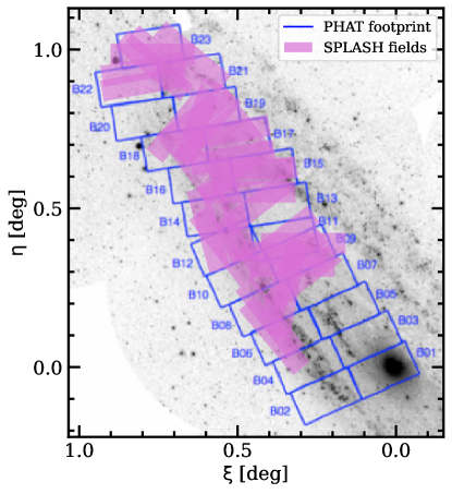
Figure 1: Location of DEIMOS fields from SPLASH (magenta patches; Section 2.2; Dorman et al. 2012, 2013, 2015) in M31-centric coordinates. The approximate size and orientation of each field is represented by a 16’ $\times$ 4’ rectangle. The outline of the PHAT footprint (Section 2.1; Dalcanton et al. 2012) is shown as blue lines. The NUV image of M31 is from the PHAT archive and was taken by GALEX.

The SPLASH survey collected $\sim$10,000 Keck/DEIMOS (Faber et al., 2003) spectra across M31’s northeastern disk to investigate its line-of-sight velocity distribution and stellar properties (Dorman et al., 2012, 2013, 2015). SPLASH stars were targeted based on a mixture of Canada-France-Hawaii Telescope (CFHT) MegaCam photometry and PHAT v1 photometry (Section 2.1). Each slitmask was observed for $\sim$1 hr using the 1200 $\ell$/mm (pre-2012 observations; Dorman et al. 2012, 2013) or 600 $\ell$/mm (post-2012 observations; Dorman et al. 2015) grating on DEIMOS.

Dorman et al. (2012, 2013, 2015) measured radial velocities from SPLASH spectra using the cross-correlation technique of Simon & Geha (2007) including A-band corrections for slit miscentering (Sohn et al., 2007) and heliocentric corrections. The typical statistical velocity uncertainty derived from the cross-correlation is roughly a few km s^-1 ($\sim$ 10 km s^-1) for spectra obtained with the 1200 (600) $\ell$/mm grating.

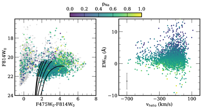
Figure 2: Membership determination for SPLASH targets with successful radial velocity measurements (Dorman et al., 2012, 2013, 2015) along the line-of-sight to M31’s disk (Section 3.1). (Left) Foreground-extinction-corrected (F475W, F814W) PHAT v2 CMD (Dalcanton et al. 2012; Williams et al. 2014; Section 2.1, 4.1) for stars with (colored points) and without (grey points) Na I $\lambda$8190 doublet equivalent width (EW_Na) measurements. We show Gyr PARSEC RGB isochrones (Marigo et al., 2017) with [Fe/H]_phot = $-2.0,-1.5,-1.0,-0.5$, 0 for reference, assuming $m-M=24.45\pm 0.05$ (Dalcanton et al., 2012). Stars with $p_{\rm Na}\leq 0.25$, which are $\geq$3 times more likely to belong to the MW foreground than M31, are classified as non-members. We also exclude stars with colors bluer than the most metal-poor RGB isochrone. (Right) EW_Na versus heliocentric velocity ($v_{\rm helio}$). We show the median uncertainty in EW_Na ($\delta$EW_Na = 2.5 Å) as a gray errorbar. Stars with $p_{\rm Na}\leq 0.25$ preferentially have blue colors or lie above the TRGB and have more positive $v_{\rm helio}$, all of which are properties characteristic of MW foreground dwarfs.

Figure 1 shows the location of SPLASH fields within the PHAT footprint. The left panel of Figure 2 shows the (F475W₀, F814W₀) color-magnitude diagram (CMD; Section 4) of 6405 stars in the SPLASH survey of M31’s disk with PHAT v2 photometry (Section 2.1) and successful radial velocity measurements. We also show Gyr PARSEC RGB isochrones (Marigo et al., 2017) spanning $-2<$ [Fe/H]_phot $<0$, assuming $m-M$ = 24.45 $\pm$ 0.05 as in Dalcanton et al. (2012). SPLASH stars span various evolutionary stages, including the upper main sequence of M31’s disk, the horizontal branch, the intermediate-age asymptotic giant branch (AGB), and the old RGB, where contamination from the MW foreground is concentrated at observed colors of F475W–F814W $\lesssim$ 2 (Dorman et al., 2015).

3 Membership and Kinematics

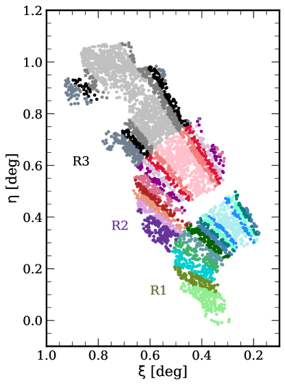
Figure 3: Location of annular radial regions (R1, R2, R3) and angular subregions in M31-centric coordinates used to model the velocity distributions (Section 3.2.1). Each point corresponds to a M31 giant star with a succesful velocity measurement from SPLASH. The regions R1, R2, and R3 are bounded by R_proj = 8, 12, and 18.5 kpc, where the kinematical parameters of the halo component in each region are fixed to the values obtained by Dorman et al. (2012). Each radial annulus is divided into angular subregions based on absolute position angle relative to the major axis (P.A. = 38^∘), where these subregions are used to constrain the disk component of the velocity distribution. Note that stars on either side of the major axis represented by the same color are part of the same subregion. Subregion designations are based on absolute angular distance from the major axis (i.e., R3₁ straddles the major axis, and R3₄ is the most distant from the major axis).

3.1 Membership

We identified MW foreground stars based on the presence of the surface-gravity sensitive Na I $\lambda$8190 Å doublet and on CMD position. The Na I doublet can discriminate between dwarf stars with strong Na I absorption features and giant stars with weak features (Schiavon et al., 1997), whereas the CMD can be used to select regions likely populated by giant stars. In total, we classified 4844 stars as M31 members.

First, we assigned stars with foreground-extinction-corrected F475W₀–F814W₀ colors (Section 4.1) bluer than the most metal-poor Gyr PARSEC RGB iscochrone (Marigo et al., 2017) by more than the photometric uncertainty to the MW foreground . These stars are substantially more likely to be intervening MW dwarfs (Gilbert et al., 2006), especially given that the SPLASH target selection procedure does not account for interstellar reddening (Section 4.1, 4.2.1) to favor a complete sample of giant star candidates. Alternatively, these blue stars may also be M31 disk stars in a different stellar evolutionary stage. SPLASH includes a large population of main-sequence turn-off stars in M31 (Figure 2), which is near the most contaminated portion of the CMD bounded by $m_{\rm F814W}<21$ and $1<m_{\rm F475W}-m_{\rm F814W}<2$ (Dorman et al., 2015).

Next, we evaluated the probability of M31 membership for stars based on their Na I equivalent widths (EW_Na) and measurement uncertainties ($\delta$EW_Na). We measured EW_Na and $\delta$EW_Na from all spectra following the method of Escala et al. (2020b). we computed the membership probabilities from likelihood ratios derived by constructing non-parametric probability distribution functions (PDFs) using EW_Na and $\delta$EW_Na measurements (assuming Gaussian uncertainties) for thousands of MW and M31 stars securely identified in the SPLASH survey of M31’s halo (e.g., Gilbert et al. 2012). The PDF weighted sample means and standard deviations are $\mu_{\rm Na,M31}$ = 0.54 Å, $\sigma_{\rm Na,M31}$ = 1.00 Å and $\mu_{\rm Na,MW}$ = 2.27 Å, $\sigma_{\rm Na,MW}$ = 1.96 Å.

Figure 2 shows the CMD of SPLASH disk stars color-coded by the EW_Na-based M31 membership probability ($p_{\rm Na}$) calculated from the PDFs. Stars with $p_{\rm Na}\leq 0.25$, which are $\geq$3 times more likely to belong to the MW foreground than M31, preferentially populate the heavily contaminated portion of the CMD identified by Dorman et al. (2015), in addition to the region above the TRGB, which has a higher incidence of contamination by bright MW foreground stars (Gilbert et al., 2006). Figure 2 also demonstrates that stars with $p_{\rm Na}\leq 0.25$ tend to have MW-like velocities ($v_{\rm helio}$_,MW $\sim-50$ km s^-1), while few of these stars are present at velocities highly consistent with M31’s stellar halo ($v_{\rm helio}$ $<-300$ km s^-1). In contrast, defining MW foreground stars by $p_{\rm Na}<0.5$, or $>$1 times more likely to belong to the MW than M31 based on EW_Na alone, would exclude many targets with CMD positions and velocities fully consistent with M31 membership. The high surface density of M31’s disk relative to the MW foreground ensures that the majority of targets are true M31 giant stars. We thus adopted $p_{\rm Na}\leq 0.25$ in addition to our CMD criterion to eliminate MW contaminants.

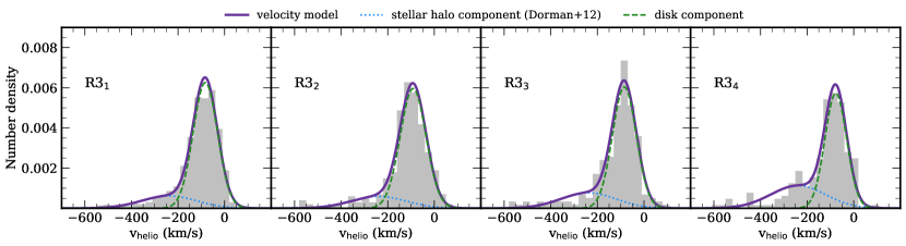
Figure 4: Heliocentric velocity distributions for region R3 (Section 3.2.1). From left to right, the panels show the velocity distribution in each subregion (grey histograms; Figure 3; Table 3.2.1), where R3₁ straddles the major axis and R3₄ is the most distant from the major axis. We also show the fitted velocity model for each subregion (thick purple lines; Section 3.2.2), which is composed of a stellar halo component (Dorman et al., 2012) with fixed mean and dispersion but variable fractional contribution (dotted blue lines) and a disk component (dashed green lines). Figures 16 and 17 show the velocity distributions and models for R1 and R2. In general, the trends between the disk component velocity and $\Delta$P.A. follow that expected for an inclined rotating disk, approaching M31’s systemic velocity ($-300$ km s^-1) with increasing $\Delta$P.A. (Dorman et al., 2012). The stellar halo component also becomes more dominant with increasing $\Delta$P.A.

This membership determination method stands in contrast to our previous work, which relied on EW_Na, calcium-triplet based metallicity, CMD position, and radial velocity to probabilistically evaluate membership for stars along the line-of-sight to M31 (e.g., Gilbert et al. 2006; Escala et al. 2020b). The primary reason that we did not use these membership determination methods is to avoid relying on transformations between HST/ACS and Johnson-Cousins photometry (e.g., Sirianni et al. 2005; Saha et al. 2011) required for Ca II triplet based metallicity calibrations (e.g., Ho et al. 2015). Additionally, we did not use radial velocity as a diagnostic measurement for membership because the velocity distribution of M31’s northeastern disk shows significant overlap with that of the MW’s disk (Ibata et al., 2005; Dorman et al., 2012). Excluding radial velocity as a diagnostic does not preclude the use of the probablistic membership determination methods, but restricts their usage to two dimensions for stars without spectroscopic metallicity measurements, such that these methods do not confer a significant advantage over the adopted approach (see Section 3.4 of Gilbert et al. 2006). Again, the high stellar surface densities of M31’s disk ensure that contamination from MW foreground stars is minimal prior to membership selection.

3.2 Velocity Distribution Modeling

Previous studies suggest that M31’s stellar velocity distribution in the disk region consists of a dynamically hot component and kinematically colder component(s) corresponding to the halo and disk respectively. To perform a chemodynamical analysis of M31’s disk, we therefore separated stars likely belonging to the disk and halo over a spatial region spanning R_proj = 4–18.5 kpc.

3.2.1 Disk Regions

Table 1: Kinematical Model Parameters for the Disk

Subregion	P.A.+,i
	P.A.+,f
	P.A.-,i
	P.A.-,f
	$\mu_{\rm disk}$
	$\sigma_{\rm disk}$
	$f_{\rm disk}$
	$N_{\rm subregion}$
R1
R11	38.0	41.9	34.1	38.0	$-$93.8${}^{+6.3}_{-6.4}$	55.6${}^{+4.7}_{-4.4}$	0.64${}^{+0.05}_{-0.05}$	219
R12	41.9	43.8	32.2	34.1	$-$117.2${}^{+7.8}_{-7.8}$	58.5${}^{+5.0}_{-4.5}$	0.78${}^{+0.06}_{-0.07}$	100
R13	43.8	45.7	30.3	32.2	$-$107.6${}^{+9.6}_{-9.5}$	60.5${}^{+6.4}_{-6.1}$	0.69${}^{+0.07}_{-0.08}$	118
R14	45.7	47.6	28.4	30.3	$-$97.5${}^{+13.5}_{-12.8}$	61.0${}^{+7.4}_{-6.9}$	0.56${}^{+0.09}_{-0.09}$	107
R15	47.6	49.8	26.2	28.4	$-$72.2${}^{+10.7}_{-10.7}$	47.6${}^{+5.5}_{-4.8}$	0.39${}^{+0.07}_{-0.07}$	112
R16	49.8	53.4	…	…	$-$108.7${}^{+9.6}_{-9.7}$	53.4${}^{+5.7}_{-5.1}$	0.57${}^{+0.08}_{-0.08}$	106
R17	53.4	57.5	…	…	$-$148.8${}^{+10.3}_{-10.1}$	60.9${}^{+7.4}_{-7.5}$	0.66${}^{+0.09}_{-0.10}$	101
R18	57.5	61.7	…	…	$-$169.7${}^{+6.9}_{-7.0}$	45.8${}^{+5.5}_{-4.6}$	0.69${}^{+0.08}_{-0.08}$	102
R19	61.7	67.7	…	…	$-$192.7${}^{+7.5}_{-7.2}$	43.5${}^{+5.7}_{-4.7}$	0.60${}^{+0.08}_{-0.08}$	107
R110	67.7	72.9	…	…	$-$204.8${}^{+6.8}_{-6.8}$	42.0${}^{+4.7}_{-4.0}$	0.59${}^{+0.08}_{-0.08}$	108
R111	72.9	92.7	…	…	$-$225.8${}^{+7.5}_{-7.4}$	45.7${}^{+4.7}_{-4.2}$	0.48${}^{+0.07}_{-0.07}$	170
R2
R21	38.0	41.8	34.2	38.0	$-$78.9${}^{+3.1}_{-3.1}$	54.3${}^{+2.4}_{-2.2}$	0.88${}^{+0.02}_{-0.02}$	421
R22	41.8	43.6	32.4	34.2	$-$89.5${}^{+4.8}_{-4.8}$	60.6${}^{+3.4}_{-3.2}$	0.90${}^{+0.03}_{-0.03}$	215
R23	43.6	45.2	30.8	32.4	$-$98.9${}^{+6.3}_{-6.3}$	59.3${}^{+4.2}_{-4.0}$	0.86${}^{+0.04}_{-0.05}$	140
R24	45.2	46.6	29.4	30.8	$-$91.6${}^{+8.0}_{-8.2}$	65.6${}^{+5.4}_{-5.0}$	0.84${}^{+0.05}_{-0.06}$	112
R25	46.6	48.4	27.6	29.4	$-$90.3${}^{+7.1}_{-7.2}$	51.6${}^{+5.3}_{-4.7}$	0.77${}^{+0.06}_{-0.06}$	104
R26	48.4	50.9	25.1	27.6	$-$99.2${}^{+6.5}_{-6.4}$	53.0${}^{+4.2}_{-3.9}$	0.83${}^{+0.05}_{-0.05}$	102
R27	50.9	52.7	…	…	$-$124.0${}^{+8.1}_{-8.5}$	55.1${}^{+5.7}_{-5.1}$	0.75${}^{+0.07}_{-0.07}$	101
R28	52.7	54.5	…	…	$-$106.8${}^{+7.3}_{-7.2}$	53.3${}^{+4.7}_{-4.2}$	0.71${}^{+0.06}_{-0.06}$	103
R29	54.5	56.4	…	…	$-$139.4${}^{+10.2}_{-10.6}$	54.9${}^{+7.4}_{-6.1}$	0.59${}^{+0.09}_{-0.09}$	103
R210	56.4	63.4	…	…	$-$142.6${}^{+7.9}_{-7.8}$	59.9${}^{+5.7}_{-5.2}$	0.68${}^{+0.07}_{-0.07}$	146
R3
R31	38.0	41.8	34.2	38.0	$-$83.0${}^{+2.0}_{-2.0}$	52.2${}^{+1.5}_{-1.4}$	0.82${}^{+0.02}_{-0.02}$	1202
R32	41.8	43.6	32.4	34.2	$-$91.2${}^{+3.8}_{-3.8}$	55.3${}^{+2.8}_{-2.6}$	0.83${}^{+0.03}_{-0.03}$	335
R33	43.6	45.1	30.9	32.4	$-$84.4${}^{+5.1}_{-5.1}$	51.1${}^{+3.8}_{-3.6}$	0.77${}^{+0.04}_{-0.05}$	195
R34	45.1	49.7	26.3	30.9	$-$77.0${}^{+4.6}_{-4.7}$	46.5${}^{+3.4}_{-3.1}$	0.67${}^{+0.04}_{-0.04}$	215

• Note. — Disk regions are based on projected radial distance: R1, R2, and R3 are bounded by R_proj = 8, 12, and 18.5 kpc. Each region is divided into subregions based on absolute angular distance from the major axis (P.A. = 38^∘; Section 3.2.1), where we indicate the positive and negative P.A. boundaries (relative to the major axis) of each symmetric subregion in degrees east of north. The parameters describing the disk component in each subregion are velocity ($\mu$), velocity dispersion ($\sigma$), and normalized fractional contribution ($f$). The stellar halo component in each region is fixed to the values determined by Dorman et al. (2012) when correcting for tidal debris. The parameter values are the 50^th percentiles of the marginalized posterior probability distributions, where the errors are calculated from the 16^th and 84^th percentiles (Section 3.2.2).

We followed the methodology of Dorman et al. (2012), where we assumed only that the stellar disk is locally cold with a symmetric velocity distribution and that each region of M31’s disk has a contribution from the inner halo. We similarly divided the disk into regions along the northeast major axis based on projected radial distance: R1, R2, and R3, which are bounded by R_proj = 8, 12, and 18.5 kpc. The median radius of stars in each bin is 6.3, 10.3, and 14.4 kpc respectively. To model the velocity distribution, we fixed the halo component in each region using the Gaussian parameters determined by Dorman et al. (2012), which are corrected for the presence of tidal debris at $v_{\rm helio}$ $<$ $-500$ km s^-1 likely related to the GSS (Fardal et al., 2013; Escala et al., 2022). The stellar halo component in regions (R1, R2, R3) is described by $\mu_{\rm halo}$ = ($-$258.2, $-$268.7, $-$238.8) km s^-1 and $\sigma_{\rm halo}$ = (134.4, 135.3, 117.5) km s^-1.

To fit for the disk component, we divided each region by position angle relative to the major axis ($\Delta$P.A.). As in Dorman et al. (2012), we defined the angle subtended by each subregion as either the $\Delta$P.A. that contains 100 stars at minimum, or the $\Delta$P.A. such that the predicted change in the line-of-sight velocity of M31’s disk ($v_{\rm obs}$) owing to $\Delta$P.A. is 10 km s^-1 (comparable to the velocity measurement precision; Section 2.2), choosing whichever was larger. As noted by Dorman et al. (2012), the predicted velocity spread due to $\Delta$P.A. within a subregion merely approximates the true spread, which is affected by additional factors such as the change in de-projected radius, deviations from perfectly circular rotation, and variations in the intrinsic local velocity distribution.

We calculated $v_{\rm obs}$ using a simple model for the perfectly circular rotation of an inclined disk (Guhathakurta et al., 1988) with inclination angle $i=77^{\circ}$ and major axis P.A. = $38^{\circ}$ given by,

$$v_{\rm obs}(\xi,\eta)=v_{\rm sys}+\frac{v_{\rm rot}\sin(i)}{\sqrt{1+\tan^{2}(\Delta{\rm P.A.})/\cos^{2}(i)}},$$ (1)

where ($\xi$, $\eta$) are M31-centric tangent plane coordinates, $v_{\rm sys}$ = $-$300 km s^-1 is the systemic velocity of M31, and $v_{\rm rot}$ = 250 km s^-1 is the disk rotation speed, which is approximately the median value measured from HI kinematics for de-projected radii in the disk plane ($R_{\rm disk}>5$ kpc; Chemin et al. 2009). Figure 3 shows the locations of the regions and subregions in M31-centric coordinates, where we divided R1, R2, and R3 into , 10, and 4 subregions, respectively. Table 3.2.1 summarizes the spatial properties of each subregion bounded by lines of constant P.A., where we designate each subregion based on absolute angular distance from the major axis.

3.2.2 Fitting for the Disk Contribution

We modeled the velocity distribution for each subregion using a two-component Gaussian mixture composed of a kinematically hot halo and colder disk (Dorman et al., 2012). The log likelihood function for a given subregion is described by,

$$\ln\mathcal{L}=\sum_{i=1}^{N_{r,s}}\ln\left(f_{s}\mathcal{N}(v_{i}|\mu_{s},\tau_{s}^{-1})+(1-f_{s})\mathcal{N}(v_{i}|\mu_{r},\tau_{r}^{-1}\right),$$ (2)

where $i$ is an index corresponding to a M31 giant star with successful velocity measurement $v_{i}$ located in subregion $s$ within region $r$ and $N_{r,s}$ is the total number of such stars. Each Gaussian distribution $\mathcal{N}$ has mean velocity $\mu$ and inverse variance $\tau=1/\sigma^{2}$, where $\mu_{r}$ and $\sigma_{r}$ are constant within a given region and correspond to the halo component. The fractional contribution of the disk, $f_{s}$, varies across subregions, where the halo fraction is constrained to $f_{r}=1-f_{s}$.

We sampled from the posterior probability distribution of Eq. 2 using an affine-invariant Markov chain Monte Carlo (MCMC) ensemble sampler (emcee; Foreman-Mackey et al. 2013) with 10² walkers and $10^{4}$ steps. We implemented flat priors for $\mu_{s}$ and $f_{s}$ over the parameter ranges of [$-600$, $+100$] km s^-1 and [0, 1], respectively. We assumed a Gamma prior on $\tau_{s}$ with $\alpha\approx 14$ and $\beta\approx 28,476$, which penalizes values of $\sigma_{s}$ below roughly 35 km s^-1 and above 70 km s^-1 based on the results of Dorman et al. (2012), and boundary conditions on $\sigma_{s}$ of [5, 150] km s^-1. We determined the kinematical parameters for the disk component in each subregion from the latter 50% of the samples, where Table 3.2.1 summarizes these parameters in terms of the 16^th, 50^th, and 84^th percentiles of the marginalized posterior distributions. Figure 4 provides an example of the velocity distribution models fit to the four subregions in region R3. We show the fits to the subregions in R1 and R2 in Appendix B.

In general, the trends between the mean velocity of the disk component and absolute $\Delta$P.A. from the major axis follow that expected for an inclined rotating disk, in agreement with Dorman et al. (2012), where the disk velocity approaches M31’s systemic velocity ($-300$ km s^-1) with increasing angular distance. This trend is not apparent in R3 (Figure 4) because it spans a smaller angular range in position angle, but this relationship is clearly visible in Table 3.2.1 (see also Figures 16 and 17 in Appendix B). We also recover that the halo component becomes more dominant with increasing angular distance from the major axis.

We emphasize that the purpose of the modeling is not to perform a detailed structural decomposition of the disk (e.g., into a thin and thick disk; Section 6.1), but rather to reliably distinguish disk stars from halo stars for the interpretation of the metallicity distributions (Section 5). As discussed by Dorman et al. (2012), the assumption of a single locally cold disk component in each subregion provides a good fit to the velocity distributions and is sufficient for a simple decomposition. We computed a probability of belonging to the disk ($p_{\rm disk}$) for M31 giant stars based on their observed velocities and positions. Using the velocity model for each star’s assigned subregion (Table 3.2.1), we calculated $p_{\rm disk}$ from likelihood ratio of the disk and halo components.

Figure 5 illustrates the spatial distribution of M31 giant stars color-coded by the disk probability, where $p_{\rm disk}$ is highest near the major axis and in the outer disk. Although the disk dominates star counts in the inner surveyed region (Courteau et al., 2011; Dorman et al., 2013), the halo’s fractional contribution to the velocity distribution is also larger at small radii, resulting in lower values of $p_{\rm disk}$. Over the SPLASH survey region, we found that 72.6% (14.4%) of M31 giant stars have a high likelihood ($p_{\rm disk}>$ 0.75, or $p_{\rm disk}<$ 0.25 for the halo) of belonging to the disk (halo). The remaining giant stars (13.0%) belong to a “mixed” population.

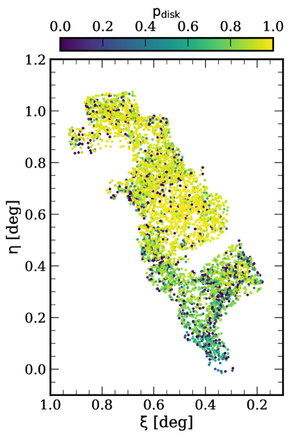
Figure 5: Location of giant stars in M31-centric coordinates, color-coded by the probability that a given star belongs to the disk versus the halo. The disk probability ($p_{\rm disk}$) is based on the velocity model for the subregion in which a star is located and its heliocentric velocity (Section 3.2.2). Stars with $p_{\rm disk}\geq 0.75$ ($p_{\rm disk}\leq 0.25$) are $\geq$3 times more likely to belong to the disk versus the halo (and vice versa).

4 Photometric Metallicity Measurement

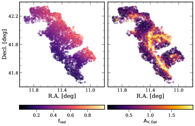
Figure 6: Sky location of M31 RGB stars in SPLASH color-coded by (left) the fraction of reddened RGB stars ($f_{\rm red}$) and (right) the median extinction ($A_{V,\rm Dal}$) from the maps of dust in M31’s disk by Dalcanton et al. (2015) (Section 4.2.1). We do not show the spread in extinction, where $\sigma_{V}\sim$ 0.30 over the entire sample. RGB stars with $\Delta$P.A. $<$ 0 (Section 3.2.1) are more likely to be reddened given that M31’s inclined thick disk is viewed in projection (J. Dalcanton et al., in preparation). The dust extinction is highest in the 10 kpc star-forming ring (Gordon et al., 2006). We used these maps to assess the impact of dust in M31’s disk on photometric metallicity measurements in Section 4.2.2.

We measured photometric metallicity for M31 RGB stars accounting for all sources of dust extinction. We determine an initial metallicity by correcting for foreground reddening in Section 4.1 and internal reddening due to M31’s gaseous disk in Section 4.2.

4.1 Initial Metallicity Determination

We first corrected the PHAT photometry (Section 2.1) for the effects of dust extinction caused by the MW foreground. We assumed $A_{V,{\rm MW}}=0.2$ for the foreground reddening, which corresponds to the median value over the low extinction PAndAS footprint (McConnachie et al., 2018) based on the dust maps by Schlegel et al. (1998) with corrections by Schlafly & Finkbeiner (2011). We used this value given that the foreground dust maps are inaccurate when restricted to M31’s disk region where its dust emission dominates over that of the MW. This translates to A${}_{\rm F814W}\sim 0.12$ and A${}_{\rm F475W}\sim 0.38$ (Gregersen et al., 2015).

We classified 3874  M31 members as red giants when correcting for foreground reddening. We defined the TRGB using 4 Gyr PARSEC isochrones (Marigo et al., 2017) spanning $-2.2<$ [Fe/H]_phot $<+0.5$. We assumed a distance modulus of $m-M=24.45\pm 0.05$. Stars were assigned to the RGB if they are below the TRGB within the photometric uncertainty: $m_{\rm F814W}+\sigma_{\rm F814W}>m_{\rm TRGB}$ (median $\sigma_{\rm F814W}$ = 0.004). The number of stars classified as red giants has a small dependence on the adopted foreground reddening, as well as the uneven reddening within M31’s disk (Section 4.2.1).

The direction of the reddening vector may result in a few young AGB stars being reddened into the RGB CMD region, but old AGB stars will not be reddened into this region owing to the shape of the TRGB. The net effect of reddening is therefore to increase the number of stars classified as red giants. The predominant, but still minimal, source of contamination in the RGB region is red helium-burning stars given that MW dwarf stars can be distinguished from genuine giant stars (Section 3.1). Contamination by red helium-burning stars would increase the number of stars in the metal-poor tails of the predominately metal-rich distributions but should not bias their median values (Section 5.1).

We determined the photometric metallicity for M31 RGB stars by interpolating de-reddened (F475W, F814W) photometry on a grid of 4 Gyr PARSEC isochrones in the relevant filters (Escala et al., 2020a). We did not extrapolate to determine [Fe/H]_phot for stars blueward of the most metal-poor isochrone, thereby introducing an effective blue limit on the RGB region.

We assumed a relatively young age for RGB stars, although the mass-weighted average age for all stellar populations in M31’s disk is 10 Gyr (Williams et al., 2015, 2017), because stars on the upper RGB are biased toward younger ages as a consequence of variable RGB lifetimes. Gregersen et al. (2015) used the star formation history measured over the PHAT footprint (Williams et al., 2015) to simulate stellar populations in M31’s disk, finding that it produced an upper RGB with a mean age of 4 Gyr. Dorman et al. (2015) found similar results for the mean RGB age when adopting a constant star formation history. If we instead assume 10 Gyr ages for RGB stars, the median difference in the photometric metallicity is $-0.22$ when accounting for foreground reddening. The assumed stellar age therefore affects the absolute metallicity scale, although we are primarily concerned with relative metallicities in this work. If the dominant halo population is systematically older than the assumed 4 Gyr old disk, the halo metallicity scale would decrease by a maximum of 0.26 (Section 6.2).

4.2 Final Metallicity Determination

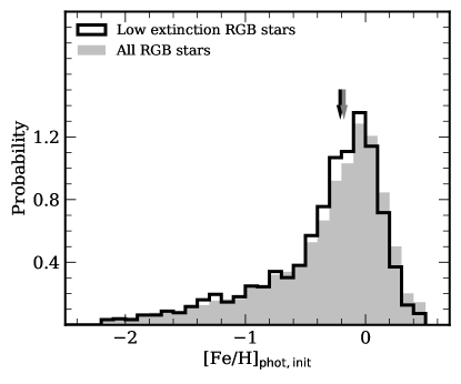
Figure 7: [Fe/H]_phot,init distributions for all RGB stars (gray filled histogram) and RGB stars located in low extinction regions of the disk (black open histogram). We measured [Fe/H]_phot,init using 4 Gyr PARSEC RGB isochrones on the foreground-reddening corrected optical CMD (Section 4). We define low extinction regions using $f_{\rm red}\times A_{V,{\rm Dal}}<0.25$ (Gregersen et al. 2015). The median [Fe/H]_phot,init for all (low extinction) RGB stars is shown as a gray (black) arrow, where [Fe/H]_{phot,init,med} = $-0.18$ ($-0.21$). This implies that most RGB stars in SPLASH are located in front of the dust layer and not significantly reddened.

In this section, we modify our initial metallicity measurement (Section 4.1), which accounts only for foreground reddening, to correct for uneven reddening due to M31’s disk. We adopt [Fe/H]_phot ([Fe/H]_phot,init) to refer to the final (inital) metallicities. We introduce the internal reddening maps and perform a preliminary assessment of dust effects on the metallicity distribution in Section 4.2.1. We describe the adopted internal extinction correction and final metallicity measurements in Section 4.2.2.

4.2.1 Internal Reddening Maps

We used the maps by Dalcanton et al. (2015), who used a novel approach to directly measure dust extinction from infrared (IR) PHAT photometry of RGB candidates assuming constant dust extinction from the MW foreground. Based on the difference between the unreddened and reddened RGB sequences over the PHAT footprint, Dalcanton et al. (2015) modeled the spatial variation in reddening using the following parameters: median extinction ($A_{V,{\rm Dal}}$), dimensionless width of the log-normal extinction distribution ($\sigma_{V}$), and the fraction of reddened stars ($f_{\rm red}$). This latter parameter reflects the geometry of the dust relative to the RGB stars, where 1$-$$f_{\rm red}$ percent of stars are assumed to be located in front of the thin dust layer of M31’s disk.

Figure 6 presents maps of $f_{\rm red}$ and $A_{V,{\rm Dal}}$ for SPLASH RGB stars obtained from 2D interpolation of each star’s position on the Dalcanton et al. dust maps. We omit showing $\sigma_{V}$ since it is relatively constant at $\sigma_{V}$ $\sim$ 0.30 over the survey region. Figure 6 shows that the value of $f_{\rm red}$ increases from the southeast to northwest edge of the survey footprint because the RGB population is located in a thick ($h_{z}$ = 0.77 kpc) and moderately inclined ($i=77^{\circ}$) disk viewed in projection (J. Dalcanton et al., in preparation), where the expected value of $f_{\rm red}$ is 50% at the major axis location (P.A. = 38^∘). The value of $A_{V,{\rm Dal}}$ is highest in the 10 kpc star forming ring (Gordon et al., 2006) but variable across the survey footprint.

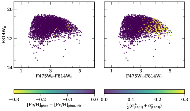
Figure 8: Foreground-reddening-corrected (F475W₀, F814W₀) CMDs for SPLASH RGB stars. The CMDs are color-coded by (left) the difference between photometric metallicity computed with ([Fe/H]_phot; Section 4.2) and without ([Fe/H]_phot,init; Section 4.1) taking into account reddening caused by dust in M31’s disk and (right) the spread in [Fe/H]_phot as quantified by the average of the 16^th ($\sigma_{\rm[Fe/H]}^{-}$) and 84^th ($\sigma_{\rm[Fe/H]}^{+}$) percentile errors of the [Fe/H]_phot distribution. We adopt [Fe/H]_phot for stars with ($\sigma_{\rm[Fe/H]}^{-}+\sigma_{\rm[Fe/H]}^{-})/2<0.03$ and exclude all other stars from the following analysis. We find that the median [Fe/H]_phot $-$ [Fe/H]_phot,init  = $-0.04$ when accounting for both their CMD and spatial positions (cf. Figure 7).

One approach to account for the effects of dust in M31’s disk is identifying RGB stars located in “low-extinction” regions. We defined low-extinction stars as those with $f_{\rm red}$ $\times$ $A_{V,{\rm Dal}}$ $<$ 0.25 following Gregersen et al. (2015), where 2054 of 3874 RGB stars meet this criterion when correcting for foreground reddening (Section 4.1). We then compared the metallicity distribution function (MDF) of RGB stars in low-extinction regions to the MDF of all RGB stars (Figure 7). The median [Fe/H]_phot,init for low-extinction RGB stars is [Fe/H]_{phot,init,med} = $-0.21$ compared to [Fe/H]_{phot,init,med} = $-0.18$ for all RGB stars. The low-extinction MDF differs most noticeably from the MDF for the full sample in the metal-rich peak, where the metal-poor tail is relatively unchanged. These small metallicity differences indicate that the majority of SPLASH RGB stars are located in front of the dust layer and not significantly reddened (see Appendix C for additional support from the IR CMDs). However, this approach is limiting given that it only considers spatial information to assess whether a star is reddened, when unreddened RGB sequences are present in the IR CMD at each location (Section 4.2.2).

4.2.2 CMD-Based Extinction Correction

We incorporated information on the optical CMD position, as opposed to solely using spatial position as in the case of the low-extinction regions (Section 4.2.1), to account for the effect of dust in M31’s disk on the metallicity determination. We constructed an extinction probability distribution for each RGB star with index $i$,

$$\begin{split}P_{i}(A_{V}|\alpha_{i},\delta_{i})&=C(f_{{\rm red},i})\times\\ &\frac{1}{A_{V}\sqrt{2\pi\sigma_{V,i}}}\exp[{-\frac{(\ln(A_{V}/A_{V,{\rm Dal},i}))^{2}}{2\sigma_{V,i}^{2}}}\Big{]}\end{split}$$ (3)

where $A_{V}$ is a variable representing $V$-band extinction, $A_{V,{\rm Dal},i}$, $\sigma_{V,i}$, and $f_{{\rm red},i}$ are the star’s dust model parameters assigned from its sky coordinates ($\alpha_{i},\delta_{i}$), and $C\in\{0,1\}$ is a constant sampled with probability {1$-f_{{\rm red},i}$, $f_{{\rm red},i}$}. We drew 10³ values of $A_{V}$ from Eq. 3 for each star, which we then converted to $A_{\rm F475W}$ and $A_{\rm F814W}$ (Section 4.1). These HST-band extinction distributions were then used with the constant $A_{V,{\rm MW}}$ to shift each star’s observed CMD position, thereby creating a statistical distribution of CMD positions corrected for all sources of dust extinction. We measured the metallicity (Section 4.1) for each corrected CMD position for each star given its fixed classification on the RGB (Section 4.1). From this distribution, we calculated a median [Fe/H]_phot value corrected for all sources of dust extinction for each star.

Figure 8 shows CMDs for RGB stars color-coded by the difference between [Fe/H]_phot and [Fe/H]_phot,init. It also shows the spread in [Fe/H]_phot as quantified by the average of the 16^th ($\sigma_{\rm[Fe/H]}^{-}$) and 84^th ($\sigma_{\rm[Fe/H]}^{+}$) percentile errors of the [Fe/H]_phot distribution. For most stars, [Fe/H]_phot is unchanged from the original [Fe/H]_phot,init value. We adopted [Fe/H]_phot as the photometric metallicity for stars with precise [Fe/H]_phot determinations (($\sigma_{\rm[Fe/H]}^{-}+\sigma_{\rm[Fe/H]}^{+})/2<0.03$), where 0.03 is the median statistical metallicity uncertainty ($\delta$[Fe/H]_phot) from the propagation of photometric uncertainties. We also incorporated the spread in [Fe/H]_phot as an error term contributing to the total metallicity uncertainty. Stars without precise [Fe/H]_phot measurements are excluded from the following analysis.

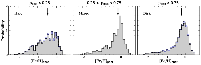
Figure 9: Metallicity distribution functions of RGB stars (black outlined gray filled histograms; Section 5.1) corrected for all sources of dust extinction ([Fe/H]_phot; Section 4.2). We separate stars into halo (left; $p_{\rm disk}$ $<$ 0.25; Section 3.2.2), mixed (middle; $0.25<$ $p_{\rm disk}$ $<0.75$), and disk (right; $p_{\rm disk}$ $>$ 0.75) populations. The bin size is 0.10, where the median $\delta$[Fe/H]_phot is 0.03. The median metallicity for each population is indicated as an arrow. For the halo, mixed, and disk populations, the median [Fe/H]_phot is $-0.46$, $-0.16$, and $-0.19$ respectively (Table 2). The dotted histogram is the resulting halo (disk) MDF in the most extreme case of contamination by metal-rich disk (metal-poor halo) interlopers (Appendix D). The blue shading defines the uncertainty region between the fiducial (solid) and contamination-corrected (dotted) MDFs. The MDFs for the disk and mixed populations are similar. The halo population is more metal-poor but still has metal-rich stars (Section 5.1).

These selection criteria reduce the RGB sample from 3874 to 3512 stars. The median difference between the final [Fe/H]_phot and original [Fe/H]_phot,init distribution is $-0.04$. We note that aside from the decrease in metallicity, the overall structure of the MDFs is unaltered, especially in the metal-poor regime. The metallicity difference is similar to that of the low extinction region selection (Figure 7). However, the approach involving Eq. 3 has the advantage of using both CMD and spatial information to construct a sample of RGB stars with relatively certain metallicity determinations despite the effects of dust in M31’s disk.

5 Chemodynamics of the Disk and Halo

In this section, we analyzed the kinematical and chemical properties of RGB stars along the line-of-sight to M31’s disk, separating them into disk, halo, and “mixed” subpopulations (Section 3.2), to ultimately investigate evolutionary scenarios for the disk and halo. We present metallicity distribution functions (MDFs) and asymmetric drift measurements for each subpopulation in Sections 5.1 and 5.2 respectively. We measure metallicity gradients for the disk and halo in Section 5.3.

5.1 Metallicity Distribution Functions

Table 2: Photometric Metallicity Distribution Properties for RGB Stars in the Halo, Mixed, and Disk Populations

Pop.	med{[Fe/H]phot}	$\langle$[Fe/H]phot$\rangle$	$\sigma${[Fe/H]phot}
Halo	$-0.46$	$-0.55\pm 0.02$	0.50
Mixed	$-0.16$	$-0.31\pm 0.02$	0.48
Disk	$-0.19$	$-0.33\pm 0.01$	0.51

• Note.— The columns are population and the simple median, mean, and standard deviation of its metallicity distribution, where [Fe/H]_phot has been corrected for all sources of dust extinction (Section 4.2). The populations are defined using the spatially and kinematically based probability that an RGB star belongs to the disk (Section 3.2.2, 5.1).

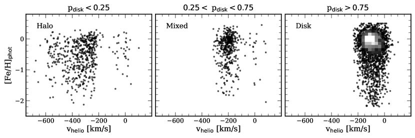
Figure 10: Photometric metallicity versus heliocentric velocity for RGB stars in SPLASH (Section 5.1). We omit showing [Fe/H]_phot and $v_{\rm helio}$ measurements uncertainties for clarity (typical values 0.03 and 5-10 km s^-1, respectively). From left to right, stars are separated into halo, mixed, and disk populations. We show a histogram in the higher density region of the disk population (bins 25 km s^-1 and 0.1). The halo population is concentrated at $v_{\rm helio}$ $\lesssim-200$ km s^-1 owing to the high likelihood that stars with $-200$ km s^-1 $\lesssim$ $v_{\rm helio}$ $\lesssim$ 0 km s^-1 belong to the dominant disk component (Table 3.2.1). Most disk stars are concentrated around [Fe/H]_phot $\sim$ $-0.10$ and $v_{\rm helio}$ $\sim$ $-100$ km s^-1, although a metal-poor tail is also present. The mixed population is dominated by stars with disk-like [Fe/H]_phot but lower $v_{\rm helio}$ $\sim$ $-200$ km s^-1. The halo shows evidence of a population with disk-like [Fe/H]_phot at $v_{\rm helio}$ $\sim$ $-280$ km s^-1 and another that is kinematically hotter and more metal-poor.

We explored the MDFs of RGB stars corrected for all sources of dust extinction (Section 4.2) in stellar halo and disk populations (Section 3.2) along the line-of-sight to M31’s disk. We defined disk (halo) stars using $p_{\rm disk}$ $>$ 0.75 ($p_{\rm disk}$ $<$ 0.25), which corresponds to stars that are at least 3 times more likely to belong to the disk (halo) based on kinematics and spatial position. We designated all other RGB stars as “mixed.” In total, 554, 458, and 2500 stars belong to the halo, mixed, and disk populations respectively. Figure 9 shows the MDFs for each population and Table 2 summarizes their properties.

The disk MDF (median [Fe/H]_phot = $-0.19$) has a dominant metal-rich population and an extended metal-poor tail. Modeling the MDF using a two-component Gaussian mixture (analogous to Section 3.2.2) yields [Fe/H]_phot = $-0.10$ ($-0.90$), $\sigma_{\rm[Fe/H]_{\rm phot}}$ = $0.23$ ($0.54$) with a fractional contribution of 71% (29%) for the metal-rich (metal-poor) disk population. The similarity between the mixed (median [Fe/H]_phot = $-0.16$) and disk MDFs implies that this intermediate population may be dominated by genuine disk stars located in subregions with larger halo fractions (Section 6.1), resulting in an uncertain separation between structural components. The halo MDF (median [Fe/H]_phot = $-0.46$) is best described by a metal-rich (metal-poor) component with [Fe/H]_phot = $-0.18$ ($-0.89$), $\sigma_{\rm[Fe/H]_{\rm phot}}$ = $0.22$ ($0.44$), and fractional contribution 48% (52%).

The presence of halo stars with similar metallicity to the disk is unusual given expectations that halos are typically metal-poor. However, the metal-rich halo population appears to be genuine, where $\lesssim$6% of metal-rich halo stars are expected to be disk interlopers. In Appendix D, we estimated this fraction by calculating the expected number of disk (halo) contaminants given the $p_{\rm disk}$-based definition for the halo (disk) population from the velocity models (Section 3.2). We then assessed the maximal impact expected on the fiducial halo (disk) MDF from contamination by metal-rich disk (metal-poor halo) stars using the MDF models (Figure 9).

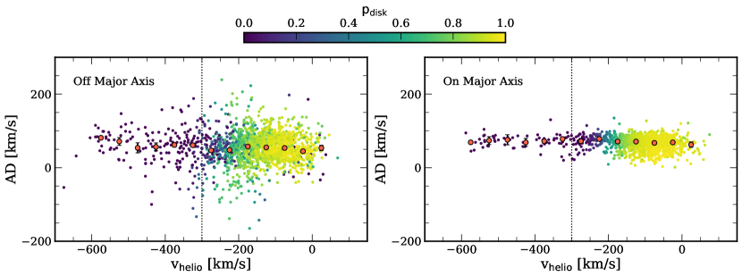
Figure 11: Asymmetric drift (AD) with respect to HI (Quirk et al., 2019) versus heliocentric velocity for SPLASH RGB stars (Section 5.2). We show stars located off (left) and on (right) the major axis, where the AD for off-axis stars exhibits more scatter due to geometrical effects. Each star is color-coded by its disk probability. The dotted line is M31’s systemic velocity. The orange points are the median AD in 50 km s^-1 $v_{\rm helio}$ bins. The variation in AD is much larger between different stellar types than within the RGB population (Quirk et al., 2019). Despite this, a clear increase in AD is visible between the disk ($p_{\rm disk}$ $>$ 0.75) and halo ($p_{\rm disk}$ $<$ 0.25) RGB populations. The metal-rich group of halo stars ($v_{\rm helio}$ $\sim$ $-280$ km s^-1, [Fe/H]_phot $\sim$ $-0.10$; Figure 10) lags the gaseous disk to a similar extent as the rest of the halo population.

Figure 10 shows the relationship between [Fe/H]_phot and $v_{\rm helio}$ for each population. The halo population is concentrated at $v_{\rm helio}$ $\lesssim-200$ km s^-1 owing to the high likelihood that stars with $-200$ km s^-1 $\lesssim$ $v_{\rm helio}$ $\lesssim$ 0 km s^-1 belong to the disk (Table 3.2.1) regardless of metallicity. Figure 10 further demonstrates that the dominant metal-rich disk population ([Fe/H]_phot $\sim$ $-0.10$ and $v_{\rm helio}$ $\sim$ $-100$ km s^-1) appears to continuously extend towards M31’s systemic velocity, where a similarly metal-rich group of stars is evident at $v_{\rm helio}$ $\sim$ $-200$ km s^-1 ($-280$ km s^-1) in the mixed (halo) population. The metal-rich halo stars mainly belong to this group, where a second kinematically hotter population encompasses the majority of the metal-poor halo stars. In order to identify stars in the metal-rich group, we modeled the halo in metallicity versus velocity space as a combination of bivariate normal distributions,

$$\mathcal{G}(v,x|\vec{\mu},\vec{\sigma})=\frac{1}{2\pi\sigma_{v}\sigma_{x}\sqrt{1-r^{2}}}\\ \times\exp\left(-\frac{1}{2(1-r^{2})}\left[\frac{(v-\mu_{v})}{\sigma_{v}^{2}}+\frac{(x-\mu_{x})}{\sigma_{x}^{2}}\right.\right.\\ \left.\left.-\frac{2r(v-\mu_{v})(x-\mu_{x})}{\sigma_{v}\sigma_{x}}\right]\right),$$ (4)

$$\mathcal{G}=f_{\rm mp}\mathcal{G}_{\rm mp}+(1-f_{\rm mp})\mathcal{G}_{\rm mr},$$ (5)

where $v$ is $v_{\rm helio}$, $x$ is [Fe/H]_phot, $\vec{\mu}=(\mu_{v},\mu_{x})$, $\vec{\sigma}=(\sigma_{v},\sigma_{x})$, and $r$ are the means, standard deviations, and correlation coefficient of the normal distribution. The halo is separated into a metal-poor population with fractional contribution $f_{\rm mp}$ and a metal-rich group with $f_{\rm mr}=1-f_{\rm mp}$. We sampled from the posterior probability distribution (Foreman-Mackey et al., 2013) of Eq. 5 to obtain $\vec{\mu}$ = ($-280.9$ $\pm$ 6.1 km s^-1, $-0.15$ $\pm$ 0.03), $\vec{\sigma}$ = (42.9 $\pm$ 4.9 km s^-1, 0.20 $\pm$ 0.02), $r$ = 0.25 $\pm$ 0.12, and $f_{\rm mr}$ = 0.26 $\pm$ 0.03 for the metal-rich group of halo stars. For the metal-poor group, we found $\vec{\mu}$ = ($-347.1$ $\pm$ 7.4 km s^-1, $-0.69$ $\pm$ 0.03), $\vec{\sigma}$ = (141.0 $\pm$ 4.9 km s^-1, 0.50 $\pm$ 0.02), and $r$ = 0.04 $\pm$ 0.05.

For each halo star, we calculated a probability of belonging to the metal-rich group, $p_{\rm mr}$, based on the likelihood ratio between $\mathcal{G_{\rm mr}}$ and $\mathcal{G_{\rm mp}}$. We assigned stars to this group if $p_{\rm mr}>0.75$, where $<$2.2% are expected to be disk interlopers (Appendix D). We further explore the properties of this interestingly metal-rich halo group—and the broader halo population—with respect to the rotation of M31’s gaseous disk in Section 5.2.

5.2 Asymmetric Drift

We examined the asymmetric drift (AD), or the difference between the gas and stellar rotation velocity at a given deprojected radius, for the various RGB subpopulations. We used AD measurements from Quirk et al. (2019) determined using SPLASH stellar velocities (Dorman et al., 2012, 2013, 2015) and HI 21 cm data (Chemin et al., 2009) in combination with a tilted ring model to derive stellar and gaseous rotation curves for M31’s disk. Quirk et al. found that AD increases with mean stellar age as traced by various stellar types, where old RGB stars (4 Gyr) lag the gas the farthest at 63.0 km s^-1. The variation in AD between stellar types is significantly larger than within the population of a given stellar type such as RGB stars (Quirk et al., 2019).

Figure 11 shows the relationship between AD and $v_{\rm helio}$ for RGB stars as defined in this work (Section 3.1, 4.1) color-coded by disk probability. We separated stars into groups on and off the major axis, where the former contains stars in subregions that straddle the major axis (i.e., with the subscript “1” ; Table 3.2.1) and the latter contains all other stars. The AD distribution for off-axis stars exhibits more scatter than those on-axis due to geometrical effects associated with measuring AD in an inclined disk (Quirk et al., 2019). Considering both on- and off-axis RGB stars, the median AD is $61.0^{+0.9}_{-0.8}$, $57.6^{+3.5}_{-2.6}$, and $66.4^{+1.5}_{-2.2}$ km s^-1 for the disk, mixed, and halo populations, respectively. At face value, this suggests that the halo and disk ADs are marginally consistent at the 1.8$\sigma$ level and that the mixed and disk populations have fully consistent ADs.

However, given the geometrical effects impacting the empirical AD measurements in areas off the major axis, the on-axis RGB stars provide a more precise representation of the underlying AD distribution. In this case, the median AD increases between the disk ($68.7^{+0.9}_{-0.8}$ km s^-1) and the mixed ($75.1^{+3.2}_{-1.4}$ km s^-1) and halo ($74.6^{+1.4}_{-1.1}$ km s^-1) populations, in accordance with expectations of dynamically colder to hotter populations. The disk and halo ADs are distinct at the 2.9$\sigma$ level, whereas the mixed population AD is consistent with the halo but differs from the disk by 2.7$\sigma$. The finding that the halo lags the gaseous disk to a greater extent than the stellar disk is likely robust given the supporting results from both the on-axis sample and full sample of RGB stars. Although the MDF of the mixed population is similar to the disk (Section 5.1), it is not immediately clear whether its AD is disk-like or halo-like. We favor the latter interpretation based on the more precise AD distribution from on-axis RGB stars, which may suggest that the mixed population is dominated by disk stars on kinematically hotter orbits (Section 6.1).

The metal-rich group of halo stars ([Fe/H]_phot $\sim$ $-0.10$) identified in Section 5.1 has a median AD of $77.4^{+0.9}_{-3.6}$ km s^-1 based on RGB tracers on the major axis and a median AD of $63.8^{+2.9}_{-1.2}$ km s^-1 based on all RGB tracers. In Figure 11, this metal-rich halo group corresponds to stars clustered near $v_{\rm helio}$ $\sim$ $-280$ km s^-1 with $p_{\rm disk}$ $<$ 0.25. For both RGB samples, the AD of the metal-rich halo group is consistent with the rest of the halo within 1$\sigma$. For the full RGB sample, the metal-rich halo group AD is However, we again interpret the on-axis ADs as being more accurate.

Thus, regardless of its disk-like metallicity, the metal-rich halo group has kinematics inconsistent with a stellar disk. We also note that despite the minor yet meaningful differences in AD, the RGB ADs are remarkably similar as a whole. This indicates that the stellar disk is almost as removed from the gaseous disk as the stellar halo, providing evidence that the disk has experienced significant dynamical disturbance(s) (Section 6.3).

5.3 Radial Metallicity Gradients

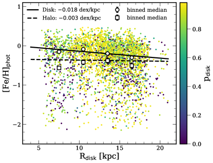
Figure 12: [Fe/H]_phot as a function of de-projected radius in the disk plane (R_disk) for SPLASH RGB stars (Section 5.3). The points are color-coded by disk probability. We determined metallicity gradients by fitting to all stars in the disk ($p_{\rm disk}$ $>$ 0.75; solid line) and halo ($p_{\rm disk}$ $<$ 0.25; dashed line) populations. We also show the median [Fe/H]_phot in radial bins for the disk (outlined circles) and halo (outlined squares). We find a gradient in the disk ($-0.018$ dex kpc^-1) and a weakly negative gradient in the halo.

We investigated whether radial metallicity gradients are present in M31’s disk and halo populations across the SPLASH survey region ($R_{\rm disk}\sim 6-18$ de-projected kpc). Based on photometry alone, M31’s disk was previously found to possess a negative metallicity gradient ($-0.020\pm 0.004$ dex kpc^-1) between $R_{\rm disk}\sim 4-20$ de-projected kpc from a sample of 7 million RGB stars in the PHAT survey (Gregersen et al., 2015). The authors accounted for photometric effects due to crowding and dust extinction, but not the effects of contamination from stars in the MW foreground or M31’s halo.

We measured the gradients using all stars in the disk ($p_{\rm disk}$ $>$ 0.75) and halo ($p_{\rm disk}$ $<$ 0.25) populations. We parameterized the gradients in terms of angles and transverse distances (Hogg et al., 2010), which we converted to traditional slopes and intercepts after sampling from the posterior probability distribution of the linear model (Foreman-Mackey et al., 2013). Figure 12 shows the relationship between $R_{\rm disk}$ and [Fe/H]_phot for RGB stars in SPLASH along with the radial gradients measured for the disk and halo. We found a slope of $-0.0176$ $\pm$ 0.0002 dex kpc^-1 for the disk, in agreement with Gregersen et al. (2015), and a weak slope of $-0.0029$ $\pm$ 0.0004 dex kpc^-1 for the halo. The associated intercept is [Fe/H]_phot = +0.037 $\pm$ 0.004 ($-0.335$ $\pm$ 0.005) for the disk (halo).

The treatment of dust extinction (Section 4) has a minor effect on the measured gradients. Using the low-extinction RGB sample defined by $f_{\rm red}$ $\times$ $A_{V,{\rm Dal}}$ $<$ 0.25 instead yields a slope of $-0.0200$ $\pm$ 0.0003 ($-0.0031$ $\pm$ 0.0005) dex kpc^-1 and an intercept of +0.092 $\pm$ 0.005 ($-0.318$ $\pm$ $0.007$) for the disk (halo). Disregarding dust in M31’s disk entirely yields a slope of $-0.0200$ $\pm$ 0.0002 ($-0.0055$ $\pm$ 0.0004) and an intercept of +0.092 $\pm$ 0.004 ($-0.269$ $\pm$ $0.005$) for the disk (halo). Our main findings of a gradient of approximately $-$0.02 dex kpc^-1 in the disk and a weakly negative gradient in the halo are therefore robust against dust effects. We adopted $-0.018^{+0.003}_{-0.001}$  as an encompassing range for the disk gradient slope.

In contrast to the slopes, the gradient intercepts are sensitive to the treatment of dust within 0.1 dex. Moreover, changes in the assumed stellar age result in absolute metallicity differences up to 0.26 (Section 4). However, the fiducial isochrone age should not affect the gradient slopes owing to the relatively constant shape of the RGB with stellar age. Instead, Gregersen et al. (2015) found that the presence of a negative age gradient with a magnitude larger than 0.1 Gyr kpc^-1 could flatten an apparent metallicity gradient in M31’s disk. Nonetheless, resolved PHAT-based star formation histories for M31’s disk do not show notable variations in the stellar age distribution with spatial position (Williams et al., 2015, 2017). Moreover, observations of massive external disk galaxies suggest that M31’s age gradient should be $\lesssim\absolutevalue{0.1}$ Gyr kpc^-1 (e.g., Sánchez-Blázquez et al. 2014; Goddard et al. 2017).

We refer the reader to Gregersen et al. (2015) for a discussion of the metallicity gradient in M31’s disk in the context of the literature. Recent developments regarding the thickness of M31’s disk (J. Dalcanton et al., in preparation) imply that this shallow radial gradient may be the result of merger-driven mixing combined with projection effects. In addition, populations of high-extinction, kinematically colder and low-extinction, kinematically hotter intermediate-age PNe along the line-of-sight to M31’s disk have been recently found to have radial argon gradients of $-0.02$ dex kpc^-1 and $-0.005$ dex kpc^-1 (Bhattacharya et al., 2022), respectively, similar to the disk and halo RGB populations in this work. We also note that, although the halo metallicity gradient is weak over the scale of the probed disk region, it is similar to the photometric metallicity gradient previously measured for the halo along the minor axis (1 dex over 100 kpc; Gilbert et al. 2014).

6 Discussion

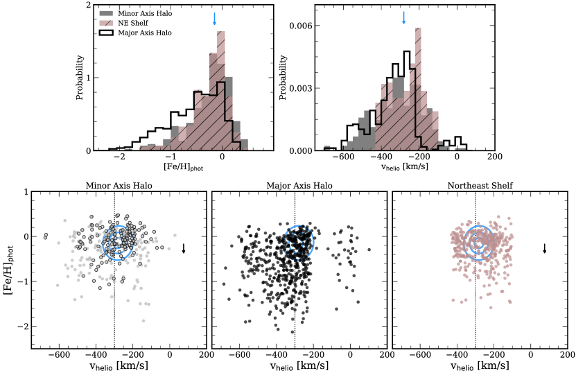
Figure 13: (Top) MDFs (left) and velocity distributions (right) for M31’s stellar halo along the minor axis (gray histograms; Gilbert et al. 2012, 2014), the major axis (black outlined histograms; this work; Dorman et al. 2012, 2013, 2015), and for the NE shelf (brown hatched histograms; Escala et al. 2022). (Bottom) Photometric metallicity versus heliocentric velocity for the minor-axis halo (left), major-axis halo (middle), and NE shelf (right). See Section 6.2 for the selection of the minor-axis halo and NE shelf samples and Section 5.1 for the major-axis halo. The outlined points (bottom left) are stars in the innermost minor axis field, f109. The systemic velocity of M31 ($-300$ km s^-1) is shown as a dotted line. We assumed 4 Gyr isochrones to compare [Fe/H]_phot between the three populations, though the mean stellar ages of the minor-axis halo and NE shelf are significantly older (Section 6.2). The black arrows in the bottom panels are the shift in [Fe/H]_phot ($-0.26$) when assuming 12 Gyr isochrones. Regardless of the assumed stellar age, the [Fe/H]_phot–$v_{\rm helio}$ distribution of the major-axis halo is distinct from the minor-axis halo and NE shelf. In particular, the pronounced cluster of stars in the major-axis halo at [Fe/H]_phot $\sim-0.10$ and $v_{\rm helio}$ $\sim$ $-280$ km s^-1 is absent from the other populations (top, blue arrows; bottom, blue contours; Section 5.1)

In this section, we place our findings on the chemodynamical properties of the disk, halo, and mixed populations (Section 5) in a broader context. We discuss the nature of the mixed population and its implications for M31’s thickened disk structure in Section 6.1. We show that the metal-rich group of halo stars (identified in Section 5.1) is inconsistent with originating from the Giant Stellar Stream merger event in Section 6.2. We also demonstrate that M31’s inner halo as probed along the major axis (i.e., near the disk) is distinct from the phase-mixed component previously studied along the minor axis (i.e., away from the disk). We put forward the hypothesis that this metal-rich halo group was kicked-up from the disk and that M31’s inner halo possesses an in-situ population similar to the MW in Section 6.3.

6.1 Disk Structure

The “mixed” population defined in Section 3.2.1, which constitutes 13.0% of the sample, consists of stars that cannot be securely associated with the stellar halo or dynamically colder disk. These stars have a disk-like MDF (Section 5.1), but kinematical properties intermediate between the disk and halo (Section 5.2). This raises the question of whether the mixed population is dominated by disk stars with uncertain kinematical classifications, potentially representing a “thicker” disk not captured by the adopted two-component velocity model (Section 3.2). Alternatively, the mixed population could simply correspond to a transition region between a uniformly thick disk and the stellar halo, possibly including kicked-up disk stars (Section 6.3).

We found that modifying the line-of-sight velocity distribution models (Section 3.2.2) to allow for a two-component disk does not result in better descriptions of the data as evaluated using Bayesian information criteria (Appendix E). Currently, evidence in favor of a multiple-component disk structure in the PHAT region is lacking. Instead, the dominant RGB population in M31’s disk region traces a thickened disk with a scale height of 0.77 kpc as probed by the fraction of reddened stars (J. Dalcanton et al., in preparation). This is substantially larger than the scale height of the integrated stellar disk of the MW (0.40 kpc; Bovy & Rix 2013) despite the relatively young age (4 Gyr; Section 4) and high metallicity ($-0.19$; Section 5.1) of M31’s disk. Moreover, the fundamentally thick nature of M31’s disk is corroborated by its large line-of-sight velocity dispersion ($\sim$50-60 km s^-1) as traced by RGB stars (Ibata et al. 2005; Dorman et al. 2012; this work) and planetary nebulae (e.g., Bhattacharya et al. 2019).

We note that the coarse relationship between velocity dispersion and metallicity found by Dorman et al. (2015) does not necessarily support a multiple-component disk structure, but rather likely reflects metallicity differences between spatial regions dominated by the stellar halo or disk. Furthermore, the thick disk component argued for by Collins et al. (2011) in the outskirts ($\gtrsim$15 kpc) of M31’s southern disk probably does not translate to the inner regions of M31’s northern disk as probed in this work (see the discussion by J. Dalcanton et al., in preparation).

We therefore favor the hypothesis that the mixed population mostly consists of stars from a thickened disk (with some halo contamination) that can be reasonably described by a single kinematical component. In general, an unambiguous kinematical detection of a multiple structural components in a projected disk would require comparisons to predicted line-of-sight velocity distributions obtained via forward modeling.

6.2 The Minor-Axis Halo and Northeast Shelf

We compared stellar populations in M31’s halo along its major axis (i.e., near the disk) to those previously studied along its minor axis (i.e., away from the disk). Our aim is to assess whether there is an evolutionary connection between the major-axis halo and disk or whether the major-axis and minor-axis halo share the same likely accretion-dominated origin (e.g., Gilbert et al. 2014; McConnachie et al. 2018; Escala et al. 2020b). We also compared the major-axis halo to the Northeast (NE) shelf, a tidal shell likely associated with the GSS (e.g., Ferguson et al. 2002, 2005; Escala et al. 2022; Dey et al. 2022), given predictions that it overlaps with the PHAT region and may therefore pollute the major-axis halo (Fardal et al., 2007, 2013). The metal-rich nature of the GSS progenitor (Gilbert et al., 2007, 2009; Ibata et al., 2007; Fardal et al., 2012; Gilbert et al., 2019; Escala et al., 2021, 2022) also raises the possibility that the metal-rich group of halo stars (Section 5.1) could correspond to GSS-related tidal debris.

We used data for the minor-axis halo (Gilbert et al., 2012, 2014) and NE shelf (Escala et al., 2022) from SPLASH. We defined the minor-axis halo using spectroscopic fields spanning 9–18 projected kpc (Gilbert et al., 2012), which covers a radial range comparable to the disk region data (4–18 projected kpc). We also excluded known kinematically cold tidal debris from the Southeast shelf (Gilbert et al., 2007) and GSS (Kalirai et al., 2006; Gilbert et al., 2009) in the minor-axis halo by requiring that a star’s probability of belonging to substructure is low ($p_{\rm sub}<0.2$, where $p_{\rm sub}$ is defined analogously to $p_{\rm disk}$ using the velocity models by Gilbert et al. 2018). For the NE shelf, we used the criterion $p_{\rm sub}>0.75$, which excludes the majority of stars suspected to be disk contaminants (Escala et al., 2022).

To eliminate the [Fe/H]_phot scale as a source of uncertainty in the comparison to the major-axis halo, we determined [Fe/H]_phot homogeneously for the minor-axis halo and NE shelf using 4 Gyr isochrones (Section 4). However, previously published [Fe/H]_phot measurements from SPLASH for these stellar structures assume 12 Gyr ages, where the mean ages of the minor-axis halo and NE shelf are 10–11 Gyr (Brown et al., 2007, 2008) and 8 Gyr (Ferguson et al., 2005; Richardson et al., 2008), respectively. Assuming 12 Gyr instead of 4 Gyr ages shifts the [Fe/H]_phot distributions by $-0.26$ dex, where the median [Fe/H]_phot = $-0.15$ and $-0.16$ for the minor-axis halo and NE shelf, respectively, in the 4 Gyr case.

We note that whether the innermost minor-axis halo field (f109) at R_proj = 9 kpc is included also impacts the associated [Fe/H]_phot distribution, where the exclusion of this field changes the median [Fe/H]_phot to $-0.29$. Although M31’s extended disk reaches beyond $R_{\rm disk}\sim 40$ kpc (Ibata et al., 2005) and is expected to have a line-of-sight velocity on the minor-axis equivalent to M31’s systemic velocity ($-300$ km s^-1), the disk fraction is predicted to be $\lesssim$10% at $R_{\rm disk}=38$ kpc in f109 (Guhathakurta et al., 2005). Furthermore, no evidence of a kinematically cold disk feature has been detected in the velocity distribution of this field (Gilbert et al., 2007; Escala et al., 2020a), so we included f109 for a more accurate representation of the minor-axis halo [Fe/H]_phot distribution over this radial range.

Figure 13 shows [Fe/H]_phot distributions, $v_{\rm helio}$ distributions, and the relationship between [Fe/H]_phot and $v_{\rm helio}$ for the minor-axis halo, major-axis halo, and NE shelf. Regardless of the adopted age, the metallicity versus velocity distribution of the major-axis halo is distinct from the minor-axis halo and NE shelf. Performing 10³ Anderson-Darling tests where the [Fe/H]_phot measurements were perturbed by their (Gaussian) uncertainties yields that the major-axis halo is inconsistent with being drawn from the same distribution as the minor-axis halo or the NE shelf at the 0.1% significance level with 95% confidence. Moreover, the pronounced cluster of major-axis halo stars at [Fe/H]_phot $\sim-0.10$ and $v_{\rm helio}$ $\sim$ $-280$ km s^-1 is missing from the other stellar structures.

Thus, M31’s major-axis halo likely contains stellar populations absent from the phase-mixed component of the minor-axis halo and not dominated by GSS-related tidal debris. Even when restricting the major-axis halo population to stars with $p_{\rm mr}<0.25$, it remains distinct from the minor-axis halo and NE shelf. This is also the case when limiting the MDFs of each stellar structure to [Fe/H]_phot $>$ $-1$, which corresponds to the RGB region in the CMD that should be entirely free of contamination by metal-rich helium burning stars (Section 4).

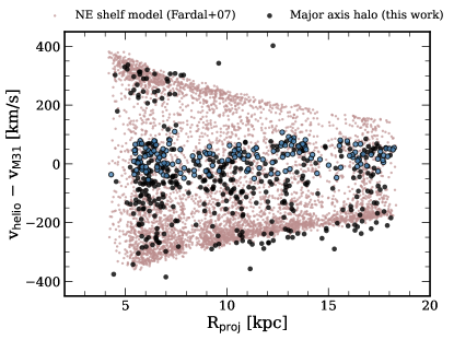
Figure 14: Heliocentric velocity shifted by M31’s systemic velocity versus projected M31-centric radius for the major-axis halo (black circles; this work) compared against model predictions for NE shelf tidal debris (red points; Fardal et al. 2007; Escala et al. 2022) at the SPLASH data location (Figure 1). Note that the model predicts M31 itself, not the NE shelf, to dominate the stars this region (Section 6.2). The metal-rich group of stars concentrated near $v_{\rm helio}$ $-$ $v_{\rm M31}$ $\sim$ km s^-1 (blue circles; $p_{\rm mr}>0.75$, Section 5.2) is inconsistent with predictions for the NE shelf, which instead should be most visible at $v_{\rm helio}$ $-$ $v_{\rm M31}$ $\lesssim$ $-$200 km s^-1 in the SPLASH disk region (Dorman et al., 2012).

We additionally evaluated whether such tidal material is likely to pollute the major-axis halo by comparing to predictions of N-body models for the formation of the GSS and NE shelf. We utilized a re-simulation of the Fardal et al. (2007) model for the complete disruption of a satellite progenitor 0.8 Gyr ago with stellar mass $M_{\rm sat}=2.2\times 10^{9}\ M_{\odot}$, which broadly provides a good match to observations of the NE shelf (Escala et al., 2022). Figure 14 shows the projected phase space distribution of the major-axis halo compared to the model predictions for NE shelf tidal debris at the location of the SPLASH disk fields (Figure 1). The model predicts that M31 host particles constitute 98.9% of the stellar material in the SPLASH survey region, with the caveat that the specific fractional contribution depends on the assumed mass ($M_{\rm host}=1.1\times 10^{11}M_{\odot}$) and structural components of the host model. We therefore expect the NE shelf to be most detectable in the SPLASH region at velocities far removed from the disk ($v_{\rm helio}$ $\sim$ $-$100 km s^-1) and along the high-density lower envelope of the tidal shell in projected phase space ($v_{\rm helio}$ $\lesssim$ $-500$ km s^-1 and R_proj $\sim 5-18$ kpc; Figure 14; see also Dorman et al. 2012). Most stars in the major-axis halo, including the metal-rich group of stars concentrated near $v_{\rm helio}$ $\sim-280$ km s^-1, are unlikely to originate from a disrupted satellite progenitor based on the expected debris pattern and the relative stellar density between M31’s disk and the putative debris.

We have established that the major-axis halo over the SPLASH survey region probably does not predominately originate in the recent accretion of the GSS progenitor in a minor merger scenario. Detailed predictions for GSS-related tidal debris in M31’s disk region in a major merger scenario (Hammer et al., 2018; D’Souza & Bell, 2018) currently remain unexplored, although any such realistic simulation must be able to broadly reproduce the shell pattern of the NE shelf (similar to Figure 14; Escala et al. 2022; Dey et al. 2022). The remaining halo formation channels involve ancient accretion and/or dissipative collapse or kinematical heating of the disk for an in-situ component. The dominant metal-poor halo population ([Fe/H]_phot $\sim$ $-0.89$; Section 5.1) may have formed via accretion or in a “classical” in-situ scenario; we discuss the possibility that the metal-rich group ($v_{\rm helio}$= $-280.9$ km s^-1, [Fe/H]_phot = $-0.15$) could have been kinematically heated from the disk by M31’s last significant merger in Section 6.3.

6.3 Kicked-Up Disk Stars

We have identified a metal-rich group of stars ($v_{\rm helio}$= $-280.9$ km s^-1, [Fe/H]_phot = $-0.15$, $f$ = 0.26; Section 5.1) in M31’s major-axis halo that lags the rotation of the gaseous disk to a similar extent as the rest of the halo population (Section 5.2). This group is inconsistent with observed and predicted properties for GSS-related tidal debris and appears to be absent from M31’s minor-axis halo (Section 6.2). M31’s bulge is too compact ($r_{b}=0.78$ kpc; Dorman et al. 2013) to contribute to stellar populations in the surveyed disk region, such that M31’s “spheroid” is indeed the stellar halo.

Based on a structural decomposition of M31’s bulge, disk, and halo using I-band surface brightness profiles, PHAT lumnosity functions, and SPLASH kinematics, Dorman et al. (2013) found statistical evidence for an excess of stars (5.2% $\pm$ 1.2%) that follow a disk-like luminosity function but have halo-like kinematics. We propose that the metal-rich group of halo stars identified in this work is the same “kicked-up” disk population. The primary difference between this work and Dorman et al. (2013) is that we performed a resolved chemodynamical analysis that is minimally dependent on model assumptions. This has enabled us to characterize M31’s putative kicked-up disk stars in detail as a distinct stellar population. These stars contribute 4.6% of the total RGB sample (see Appendix D for the small effect of disk interlopers). Using the fractional contributions from Table 3.2.1, the total statistical fraction of disk RGB stars in the sample is $74.9\%\pm 4.5$%. The estimated kicked up disk fraction is therefore $5.7\%\pm 0.2\%$.

The chemical and kinematical properties of these metal-rich halo stars are broadly consistent with predictions of heated disk populations in similations of in-situ stellar halo formation. As noted by Dorman et al. (2013), Purcell et al. (2010) found that $\sim$1% of stars should be heated into the halo from the disk by a minor merger at a low impact angle, which is comparable to but systematically lower than estimates of the kicked-up disk fraction in M31. Moreover, stars heated from the disk can fractionally constitute $\sim$30% of the inner stellar halo (e.g., Tissera et al. 2013; Cooper et al. 2015; Khoperskov et al. 2022) as found in this work. Based on simulations including both major and minor mergers, Jean-Baptiste et al. 2017 found that kicked-up disk populations can appear structured in kinematical phase space and should exhibit some degree of rotation inversely correlated with total accreted mass. Although other studies have similarly found that disk heated stars may show signs of rotational support, there can be significant halo-to-halo scatter (e.g., McCarthy et al. 2012; Tissera et al. 2013). M31’s metal-rich clump of halo stars has a similar degree of rotational support as the rest of the dynamically hot halo population (Section 5.2), where M31’s inner halo slowly rotates (Dorman et al., 2012).

6.3.1 Comparison to the MW

In the MW, stars born in the proto-disk but kinematically heated onto high-eccentricity orbits by early merger(s) constitute the sole in-situ component of the stellar halo (e.g., Bonaca et al. 2017; Haywood et al. 2018; Di Matteo et al. 2019; Belokurov et al. 2020). In particular, the formation of in-situ halo, or “Splash”, has been connected to the the Gaia-Enceladus-Sausage merger event (GES; e.g., Helmi et al. 2018; Belokurov et al. 2018; Gallart et al. 2019; Bonaca et al. 2020; Grand et al. 2020). This in-situ halo component has chemical abundances similar to the thick disk (e.g., Di Matteo et al. 2019; Belokurov et al. 2020; Naidu et al. 2020), old stellar ages comparable to the accreted component of the stellar halo (e.g., Gallart et al. 2019; Bonaca et al. 2020), and smoothly transitions in metallicity versus velocity space from the thin and thick disks (e.g., Belokurov et al. 2020). Furthermore, it fractionally constitutes $<$15% of the MW’s stellar halo for disk heights above 2 kpc (Naidu et al., 2020).

Although we cannot perform one-to-one comparisons with the MW’s stellar halo, our results suggest that M31 may possess a fractionally larger (28.9% of halo RGB stars; Section 5.1) in-situ halo component than the MW. In contrast to M31, the MDF of the MW’s inner halo is strongly bimodal due to in-situ ([Fe/H] $\sim$ $-0.5$) and accreted ([Fe/H] $\sim$ $-1.2$) components dominated by the Splash and the GES merger remnant respectively (e.g., Bonaca et al. 2017; Di Matteo et al. 2019). However, given M31’s more active merger history (e.g., McConnachie et al. 2018), there is no apriori reason to expect M31’s inner halo to exhibit the same metallicity signatures as the MW. In simulations of stellar halo formation, the in-situ halo is generally more metal-rich than the accreted component (Zolotov et al., 2009; Font et al., 2011; Tissera et al., 2012, 2013, 2014; Cooper et al., 2015; Pillepich et al., 2015; Khoperskov et al., 2022), but otherwise halo MDFs can vary owing to scatter in formation histories.

7 Summary

We have combined optical HST photometry from PHAT with Keck/DEIMOS spectra from SPLASH to execute the first large-scale chemodynamical analysis of M31’s inner disk region (4–19 kpc) based on metallicity and velocity measurements for 3512 RGB stars. We have performed a kinematical decomposition as a function of position across the disk region, where the line-of-sight velocity distributions are well-described by the combination of a thick stellar disk and stellar halo. As originally found by Dorman et al. (2012), the disk-dominated (72.6% of RGB stars) region nevertheless has a substantial contribution from the inner stellar halo (14.4% of RGB stars) and an intermediate population with uncertain disk-halo classification (13.0% of RGB stars). We have further found that:

1. Assuming 4 Gyr stellar ages, the disk is characterized by a dominant metal-rich population (median [Fe/H]_phot = $-0.19$ when corrected for dust effects; Section 4, 5.1). The stellar halo is more metal-poor ([Fe/H]_phot= $-0.46$), but contains a non-negligible fractional contribution ($f$ = 0.26) from a stellar population with disk-like metallicity ([Fe/H]_phot = $-0.15$) that appears as a continuous extension of the disk in velocity space ($v_{\rm helio}$ = $-280.9$ km s^-1).

2. The AD, or rotational lag between the stellar and gaseous disks, is similar between the disk ($68.7^{+0.9}_{-0.8}$ km s^-1) and halo ($74.6^{+1.4}_{-1.1}$ km s^-1) populations (Quirk et al. 2019; Section 5.2), suggesting that the disk has experienced significant dynamical heating. Despite this similarity, the halo AD is inconsistent with the disk, and the metal-rich halo stars have an AD ($77.4^{+0.9}_{-3.6}$ km s^-1) consistent with the rest of the halo, suggesting that it does not correspond to a canonical thick disk.

3. The disk metallicity gradient is $-0.018^{+0.003}_{-0.001}$ dex kpc^-1, in agreement with Gregersen et al. (2015). This shallow gradient may originate from merger-driving mixing combined with projection effects. The halo metallicity gradient is similar to that measured over 100 kpc scales along the minor axis (Gilbert et al., 2014) at $-0.003^{+0.003}_{-0.001}$ dex kpc^-1 (Section 5.3).

4. RGB stars with uncertain disk-halo classifications have a disk-like MDF (Section 5.1) and AD intermediate between the disk and halo (Section 5.2). Rather than corresponding to a second thicker disk component, this mixed population is likely dominated by stars from a single thickened disk as it transitions into a stellar halo (Section 6.1).

5. The MDF of M31’s inner halo along the major axis (i.e., near the disk) is distinct from the halo MDF probed along the minor axis (i.e., away from the disk) over an equivalent radial range (Section 6.2). The metallicity and projected phase space properties of the metal-rich major-axis halo stars are also inconsistent with observations of the Northeast shelf and predictions for GSS-related tidal debris in a minor merger scenario (Fardal et al. 2007; Escala et al. 2022). This indicates that they were probably not accreted onto the halo.

6. The chemical and kinematical properties of the metal-rich halo stars (Section 5.1, 5.2) broadly agree with predictions of heated disk populations and some expectations for an in-situ halo based on current knowledge of the MW (Section 6.3). The estimated fraction of kicked-up disk stars is $5.7\%\pm 0.2\%$ of RGB stars in the surveyed region, in agreement with the statistically inferred value of 5.2% $\pm$ 1.2% from Dorman et al. (2013).

These findings point to a scenario in which M31’s inner stellar halo along the major-axis is distinct from the minor-axis halo, implying potentially disparate origins for each stellar structure. In particular, the minor-axis halo may be dominated by accretion from the GSS merger and more ancient events (e.g., Brown et al. 2006; Gilbert et al. 2007, 2014; Ibata et al. 2014; McConnachie et al. 2018; Escala et al. 2020b; Dey et al. 2022), whereas the metal-rich nature of the major-axis halo and the thickened nature of the disk suggests an entangled evolutionary history potentially driven by merger(s) and subsequent disk heating.

Appendix A Milky Way Foreground Contamination

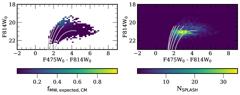
Figure 15: (Left) The fraction of expected MW contaminants (Eq. LABEL:eq:fcontam) in the M31 giant star region of the CMD, defined using the CMD membership criterion from Section 3.1. We show 4 Gyr PARSEC RGB isochrones (gray lines) for reference as in Figure 2. The most contaminated portion of the CMD corresponds to relatively blue stars above the TRGB. (Right) The number density of M31 giant stars in SPLASH, classified using the CMD criterion (i.e., without EW_Na measurements; Section 3.1). There are few SPLASH stars in the contaminated portion of the CMD (see also Figure 2). We expect $\sim$0.2% of SPLASH stars to be MW contaminants based on CMD information alone.

Appendix B Velocity Models for Additional Regions

Here, we show the velocity distributions and model fits (Section 3.2) for regions R1 (Figure 16) and R2 (Figure 17) for completion.

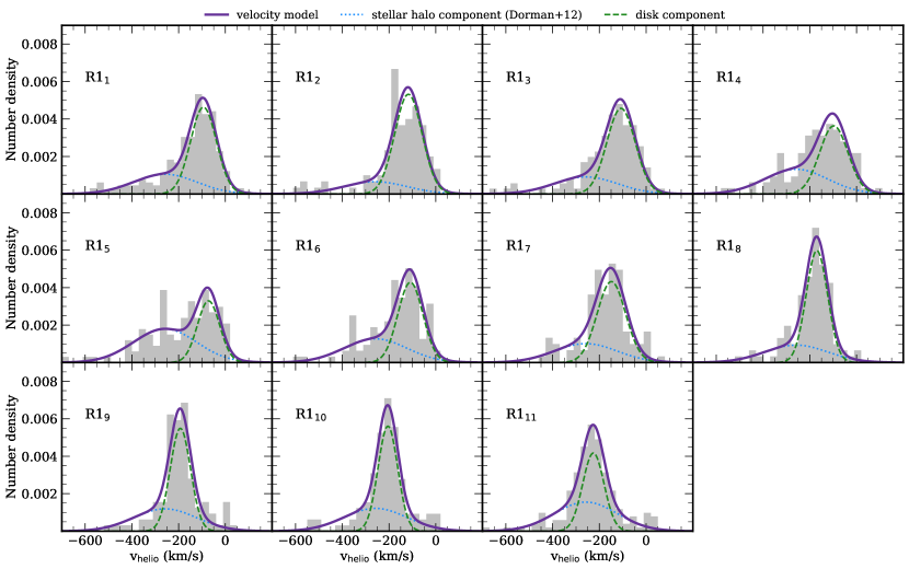
Figure 16: Same as Figure 4, except for region R1.

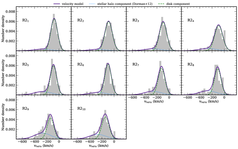
Figure 17: Same as Figure 4, except for region R2.

Appendix C Infrared Color-Magnitude Diagram

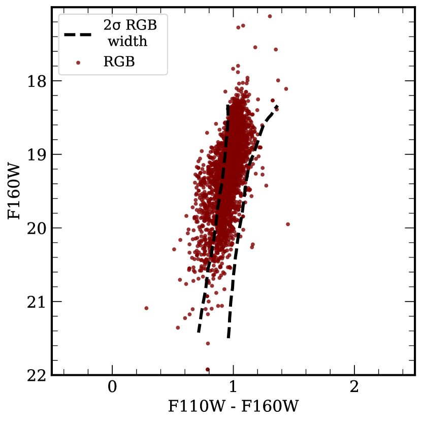
Figure 18: IR (F110W, F160W) PHAT v2 CMD (Dalcanton et al., 2012; Williams et al., 2014) for RGB stars in SPLASH (Appendix C). The RGB classification is based on the foreground-reddening corrected optical CMD (Section 4.1). The RGB stars follow a tight sequence insensitive to metallicity and age. Note that the axes are not shown to equal scale for clarity. The black dashed lines are the estimated 2$\sigma$ width expected for an unreddened RGB CMD, taking into account stellar surface density variations (Dalcanton et al., 2015). The lack of second broader sequence at redder colors suggests that the majority of stars are in front of the dust layer and not significantly reddened.

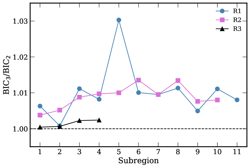
Figure 19: The ratio between the Bayesian information criterion (BIC) for the three-component and two-component velocity models for the line-of-sight velocity distribution of each subregion (Appendix E). The blue, magenta, and black lines correspond to radial regions R1, R2, and R3 respectively (Section 3.2.1). The dashed horizontal line is unity. For subregions, M31’s disk is well-described by a single thickened component (BIC₂ $<$ BIC₃). Regardless, the similarity between the BIC values indicates that a simpler two-component model (halo, thick disk) is preferred.

Figure 19 shows the observed PHAT v2 (F110W, F160W) CMD of RGB stars in SPLASH classified using the foreground-reddening corrected optical CMD (Section 4.1). The IR CMD consists of a tight sequence of unreddened stars, where this sequence is largely insensitive to age and metallicity variations, although it is weakly dependent on stellar surface density due to the effect of crowding on the photometry (Dalcanton et al., 2015). We note that the apparent excess of blue stars in Figure 19 is partly a consequence of the unequal axes scales. This blue population corresponds to metal-poor RGB stars (Section 5.1) and a small number of red helium burning stars (Section 4.1). The lack of a second broader sequence at redder colors in Figure 19 implies that the majority of RGB stars in SPLASH are in front of the thin dust layer of M31’s disk, in agreement with results from the low-extinction MDF (Figure 7).

Appendix D Structural Population Contamination

The presence of non-negligible groupings of metal-poor and metal-rich stars in the disk and halo (Section 5.1), respectively, raises the question of how much contamination from halo star interlopers is expected in the disk population ($f_{\rm contam}^{\rm disk}$) and vice versa for the halo population ($f_{\rm contam}^{\rm halo}$). We defined the halo (disk) populations using the threshold $p_{\rm disk}$ $<$ 0.25 ($p_{\rm disk}$ $>$ 0.75) as in Section 3.2.2. We computed $f_{\rm contam}^{\rm disk}$ and $f_{\rm contam}^{\rm halo}$ using the halo and disk component velocity models for each subregion $s$ in radial region $r$ (Eq. 2, Section 3.2).

The $p_{\rm disk}$ $>$ 0.75 criterion for disk stars corresponds to a bounded velocity range within each subregion ([$v_{\rm lo,disk}$, $v_{\rm hi,disk}$]) and conversely the $p_{\rm disk}$ $<$ 0.25 criterion for halo stars corresponds to a set of unbounded ranges at the extrema of a subregion’s velocity distribution ([$-\infty$, $v_{\rm lo,halo}$] and [$v_{\rm hi,halo}$, $\infty$]). For each subregion, we calculated the expected ratio of halo stars to disk stars ($\mathcal{R}_{r,s}$) in the “disk” velocity range and “halo” velocity ranges by integrating the velocity models over each domain. That is, for the disk velocity range,

$$\mathcal{R}_{r,s}^{\rm disk}=\frac{\int_{v_{\rm lo,disk}}^{v_{\rm hi,disk}}(1-f_{s})\mathcal{N}_{r}(v)dv}{\int_{v_{\rm lo,disk}}^{v_{\rm hi,disk}}f_{s}\mathcal{N}_{s}(v)dv},$$ (D1)

where the velocity models are defined as in Eq. 2 given the parameters in Table 3.2.1. Analagously for the halo velocity ranges,

$$\mathcal{R}_{r,s}^{\rm halo}=\frac{\int_{-\infty}^{v_{\rm lo,halo}}(1-f_{s})\mathcal{N}_{r}(v)dv+\int_{v_{\rm hi,halo}}^{\infty}(1-f_{s})\mathcal{N}_{r}(v)dv}{\int_{-\infty}^{v_{\rm lo,halo}}f_{s}\mathcal{N}_{s}(v)dv+\int_{v_{\rm hi,halo}}^{\infty}f_{s}\mathcal{N}_{s}(v)dv}.$$ (D2)

Based on the number of stars in each subregion ($N_{r,s}$), we converted $\mathcal{R}_{r,s}^{\rm disk}$ to an expected number of halo stars, $N_{r,s,h}^{\rm disk}$, and analogously for $\mathcal{R}_{r,s}^{\rm halo}$. Thus, $f_{\rm contam}^{\rm disk}$ is given by the expected number of interlopers in each subregion summed over the survey footprint,

$$\sum_{r}\sum_{s}N_{r,s,h}^{\rm disk}/(N_{r,s,h}^{\rm disk}+(1-\mathcal{R}_{r,s}^{\rm disk})\times N_{r,s})$$ (D3)

where $f_{\rm contam}^{\rm halo}$ is the complementary formulation. This yields $f_{\rm contam}^{\rm disk}$ = 7.8% and $f_{\rm contam}^{\rm halo}$ = 7.4%.

These contamination fractions indicate that the metal-poor disk and metal-rich halo populations, which have fractional contributions to the disk and halo MDFs of 29% and 48% respectively, cannot be solely explained by interlopers originating from a predominantly metal-poor halo or metal-rich disk. This is particularly unlikely for the metal-poor disk population owing to the high density of metal-poor stars with disk-like velocities (Figure 10). We estimated the maximal effect of metal-rich disk (metal-poor halo) interlopers on the halo (disk) MDF by subtracting the approximate number of stars corresponding to $f_{\rm contam}^{\rm halo}$ ($f_{\rm contam}^{\rm disk}$) from the halo (disk) sample. The stars are probabilistically removed according to their metallicity and the metal-rich (metal-poor) component model of the disk (halo) MDF, which we assumed to represent a “true” metal-rich disk (metal-poor halo) population. We performed 10³ iterations to obtain a distribution on each statistical quantity, finding that the median and mean on [Fe/H]_phot becomes $-0.50^{+0.003}_{-0.002}$ ($-0.17^{+0.001}_{-0.003}$) and $-0.58\pm 0.002$ ($-0.31\pm 0.002$) for the halo (disk) population (cf. Table 2). This corresponds a difference of $-0.08$ ($-0.05$) in the median (mean) metallicity of the halo, whereas the values for the disk are unchanged.

Figure 9 shows the effect on the fiducial halo (disk) MDF in the extremal case of contamination by disk (halo) interlopers. The halo MDF shape is affected more than the disk, although the halo population retains a significant contribution from stars with disk-like [Fe/H]_phot. The fraction of stars assigned to the metal-rich halo component based on a simple likelihood ratio definition decreases from 52.9% to 49.3% for the fiducial and contamination-corrected halo MDFs, respectively. We therefore do not expect more than 3.6% of metal-rich halo stars to be disk interlopers. Moreover, the fraction of stars assigned to the metal-rich halo group using the criterion $p_{\rm mr}>0.75$ decreases from 28.9% to 26.7% in the case of this comparison.

Appendix E Three-Component Velocity Models

To test whether the line-of-sight velocity distributions provide statistical evidence in favor of a two-component disk structure in M31 (Section 6.1), we fit the velocity distributions for each subregion with a three-component model nominally composed of a halo, thick disk, and thin disk. The likelihood function in this case is therefore,

$$\ln\mathcal{L}=\sum_{i=1}^{N_{r,s}}\ln\left(f_{s_{1}}\mathcal{N}(v_{i}|\mu_{s_{1}},\tau_{s_{1}}^{-1})+f_{s_{2}}\mathcal{N}(v_{i}|\mu_{s_{2}},\tau_{s_{2}}^{-1})+(1-f_{s_{1}}-f_{s_{2}})\mathcal{N}(v_{i}|\mu_{r},\tau_{r}^{-1}\right),$$ (E1)

in comparison to Eq. 2. We required that $\mu_{s_{1}}>\mu_{s_{2}}$, $\sigma_{s_{1}}<\sigma_{s_{2}}$, $f_{s_{1}}>f_{s_{2}}$ for primary thin and secondary thick disk components, but otherwise retained the same assumptions and procedure as in Section 3.2.2. We evaluated the goodness-of-fit of the three-component and two-component velocity models for each subregion using the Bayesian information criterion (BIC; Figure 19). For subregion, we found that a two-component model consisting of a halo and single thickened disk component provides a better description of the data. Regardless, the similarity between the BIC values indicates that a simpler two-component model provides an adequate statistical description of the data compared to a three-component model.

References

- Abadi et al. (2003) Abadi, M. G., Navarro, J. F., Steinmetz, M., et al. 2003, ApJ, 597, 21. doi:10.1086/378316
- Arnaboldi et al. (2022) Arnaboldi, M., Bhattacharya, S., Gerhard, O., et al. 2022, arXiv:2208.02328
- Astropy Collaboration et al. (2013) Astropy Collaboration, Robitaille, T. P., Tollerud, E. J., et al. 2013, A&A, 558, A33. doi:10.1051/0004-6361/201322068
- Astropy Collaboration et al. (2018) Astropy Collaboration, Price-Whelan, A. M., Sipőcz, B. M., et al. 2018, AJ, 156, 123. doi:10.3847/1538-3881/aabc4f
- Bhattacharya et al. (2019) Bhattacharya, S., Arnaboldi, M., Caldwell, N., et al. 2019, A&A, 631, A56. doi:10.1051/0004-6361/201935898
- Bhattacharya et al. (2022) Bhattacharya, S., Arnaboldi, M., Caldwell, N., et al. 2022, arXiv:2203.06428
- Belokurov et al. (2018) Belokurov, V., Erkal, D., Evans, N. W., et al. 2018, MNRAS, 478, 611. doi:10.1093/mnras/sty982
- Belokurov et al. (2020) Belokurov, V., Sanders, J. L., Fattahi, A., et al. 2020, MNRAS, 494, 3880. doi:10.1093/mnras/staa876
- Bernard et al. (2015) Bernard, E. J., Ferguson, A. M. N., Richardson, J. C., et al. 2015, MNRAS, 446, 2789. doi:10.1093/mnras/stu2309
- Bonaca et al. (2017) Bonaca, A., Conroy, C., Wetzel, A., et al. 2017, ApJ, 845, 101. doi:10.3847/1538-4357/aa7d0c
- Bonaca et al. (2020) Bonaca, A., Conroy, C., Cargile, P. A., et al. 2020, ApJ, 897, L18. doi:10.3847/2041-8213/ab9caa
- Bournaud et al. (2009) Bournaud, F., Elmegreen, B. G., & Martig, M. 2009, ApJ, 707, L1. doi:10.1088/0004-637X/707/1/L1
- Bovy et al. (2012) Bovy, J., Rix, H.-W., & Hogg, D. W. 2012, ApJ, 751, 131. doi:10.1088/0004-637X/751/2/131
- Bovy & Rix (2013) Bovy, J. & Rix, H.-W. 2013, ApJ, 779, 115. doi:10.1088/0004-637X/779/2/115
- Brook et al. (2004) Brook, C. B., Kawata, D., Gibson, B. K., et al. 2004, ApJ, 612, 894. doi:10.1086/422709
- Brown et al. (2006) Brown, T. M., Smith, E., Ferguson, H. C., et al. 2006, ApJ, 652, 323. doi:10.1086/508015
- Brown et al. (2007) Brown, T. M., Smith, E., Ferguson, H. C., et al. 2007, ApJ, 658, L95. doi:10.1086/515395
- Brown et al. (2008) Brown, T. M., Beaton, R., Chiba, M., et al. 2008, ApJ, 685, L121. doi:10.1086/592686
- Chemin et al. (2009) Chemin, L., Carignan, C., & Foster, T. 2009, ApJ, 705, 1395. doi:10.1088/0004-637X/705/2/1395
- Chiba & Beers (2000) Chiba, M. & Beers, T. C. 2000, AJ, 119, 2843. doi:10.1086/301409
- Collins et al. (2011) Collins, M. L. M., Chapman, S. C., Ibata, R. A., et al. 2011, MNRAS, 413, 1548. doi:10.1111/j.1365-2966.2011.18238.x
- Cooper et al. (2012) Cooper, M. C., Griffith, R. L., Newman, J. A., et al. 2012, MNRAS, 419, 3018
- Cooper et al. (2015) Cooper, A. P., Parry, O. H., Lowing, B., et al. 2015, MNRAS, 454, 3185. doi:10.1093/mnras/stv2057
- Courteau et al. (2011) Courteau, S., Widrow, L. M., McDonald, M., et al. 2011, ApJ, 739, 20. doi:10.1088/0004-637X/739/1/20
- D’Souza & Bell (2018) D’Souza, R. & Bell, E. F. 2018, Nature Astronomy, 2, 737. doi:10.1038/s41550-018-0533-x
- Dalcanton et al. (2012) Dalcanton, J. J., Williams, B. F., Lang, D., et al. 2012, ApJS, 200, 18. doi:10.1088/0067-0049/200/2/18
- Dalcanton et al. (2015) Dalcanton, J. J., Fouesneau, M., Hogg, D. W., et al. 2015, ApJ, 814, 3. doi:10.1088/0004-637X/814/1/3
- Dey et al. (2022) Dey, A., Najita, J. R., Koposov, S. E., et al. 2022, arXiv:2208.11683
- Di Matteo et al. (2019) Di Matteo, P., Haywood, M., Lehnert, M. D., et al. 2019, A&A, 632, A4. doi:10.1051/0004-6361/201834929
- Dorman et al. (2012) Dorman, C. E., Guhathakurta, P., Fardal, M. A., et al. 2012, ApJ, 752, 147. doi:10.1088/0004-637X/752/2/147
- Dorman et al. (2013) Dorman, C. E., Widrow, L. M., Guhathakurta, P., et al. 2013, ApJ, 779, 103. doi:10.1088/0004-637X/779/2/103
- Dorman et al. (2015) Dorman, C. E., Guhathakurta, P., Seth, A. C., et al. 2015, ApJ, 803, 24. doi:10.1088/0004-637X/803/1/24
- Escala et al. (2020a) Escala, I., Gilbert, K. M., Kirby, E. N., et al. 2020, ApJ, 889, 177. doi:10.3847/1538-4357/ab6659
- Escala et al. (2020b) Escala, I., Kirby, E. N., Gilbert, K. M., et al. 2020, ApJ, 902, 51. doi:10.3847/1538-4357/abb474
- Escala et al. (2021) Escala, I., Gilbert, K. M., Wojno, J., et al. 2021, AJ, 162, 45. doi:10.3847/1538-3881/abfec4
- Escala et al. (2022) Escala, I., Gilbert, K. M., Fardal, M., et al. 2022, arXiv:2203.16675
- Faber et al. (2003) Faber, S. M., Phillips, A. C., Kibrick, R. I., et al. 2003, Proc. SPIE, 4841, 1657. doi:10.1117/12.460346
- Fardal et al. (2012) Fardal, M. A., Guhathakurta, P., Gilbert, K. M., et al. 2012, MNRAS, 423, 3134. doi:10.1111/j.1365-2966.2012.21094.x
- Fardal et al. (2007) Fardal, M. A., Guhathakurta, P., Babul, A., et al. 2007, MNRAS, 380, 15. doi:10.1111/j.1365-2966.2007.11929.x
- Fardal et al. (2013) Fardal, M. A., Weinberg, M. D., Babul, A., et al. 2013, MNRAS, 434, 2779. doi:10.1093/mnras/stt1121
- Ferguson et al. (2002) Ferguson, A. M. N., Irwin, M. J., Ibata, R. A., et al. 2002, AJ, 124, 1452. doi:10.1086/342019
- Ferguson et al. (2005) Ferguson, A. M. N., Johnson, R. A., Faria, D. C., et al. 2005, ApJ, 622, L109. doi:10.1086/429371
- Font et al. (2011) Font, A. S., McCarthy, I. G., Crain, R. A., et al. 2011, MNRAS, 416, 2802. doi:10.1111/j.1365-2966.2011.19227.x
- Forbes et al. (2012) Forbes, J., Krumholz, M., & Burkert, A. 2012, ApJ, 754, 48. doi:10.1088/0004-637X/754/1/48
- Foreman-Mackey et al. (2013) Foreman-Mackey, D., Hogg, D. W., Lang, D., et al. 2013, PASP, 125, 306. doi:10.1086/670067
- Gallart et al. (2019) Gallart, C., Bernard, E. J., Brook, C. B., et al. 2019, Nature Astronomy, 3, 932. doi:10.1038/s41550-019-0829-5
- Gilbert et al. (2006) Gilbert, K. M., Guhathakurta, P., Kalirai, J. S., et al. 2006, ApJ, 652, 1188. doi:10.1086/508643
- Gilbert et al. (2007) Gilbert, K. M., Fardal, M., Kalirai, J. S., et al. 2007, ApJ, 668, 245. doi:10.1086/521094
- Gilbert et al. (2009) Gilbert, K. M., Guhathakurta, P., Kollipara, P., et al. 2009, ApJ, 705, 1275. doi:10.1088/0004-637X/705/2/1275
- Gilbert et al. (2012) Gilbert, K. M., Guhathakurta, P., Beaton, R. L., et al. 2012, ApJ, 760, 76. doi:10.1088/0004-637X/760/1/76
- Gilbert et al. (2014) Gilbert, K. M., Kalirai, J. S., Guhathakurta, P., et al. 2014, ApJ, 796, 76. doi:10.1088/0004-637X/796/2/76
- Gilbert et al. (2018) Gilbert, K. M., Tollerud, E., Beaton, R. L., et al. 2018, ApJ, 852, 128. doi:10.3847/1538-4357/aa9f26
- Gilbert et al. (2019) Gilbert, K. M., Kirby, E. N., Escala, I., et al. 2019, ApJ, 883, 128. doi:10.3847/1538-4357/ab3807
- Goddard et al. (2017) Goddard, D., Thomas, D., Maraston, C., et al. 2017, MNRAS, 466, 4731. doi:10.1093/mnras/stw3371
- Gordon et al. (2006) Gordon, K. D., Bailin, J., Engelbracht, C. W., et al. 2006, ApJ, 638, L87. doi:10.1086/501046
- Grand et al. (2020) Grand, R. J. J., Kawata, D., Belokurov, V., et al. 2020, MNRAS, 497, 1603. doi:10.1093/mnras/staa2057
- Gregersen et al. (2015) Gregersen, D., Seth, A. C., Williams, B. F., et al. 2015, AJ, 150, 189. doi:10.1088/0004-6256/150/6/189
- Guhathakurta et al. (1988) Guhathakurta, P., van Gorkom, J. H., Kotanyi, C. G., et al. 1988, AJ, 96, 851. doi:10.1086/114851
- Guhathakurta et al. (2005) Guhathakurta, P., Ostheimer, J. C., Gilbert, K. M., et al. 2005, astro-ph/0502366
- Guhathakurta et al. (2006) Guhathakurta, P., Rich, R. M., Reitzel, D. B., et al. 2006, AJ, 131, 2497. doi:10.1086/499562
- Hammer et al. (2018) Hammer, F., Yang, Y. B., Wang, J. L., et al. 2018, MNRAS, 475, 2754. doi:10.1093/mnras/stx3343
- Harris et al. (2020) Harris, C. R., Millman, K. J., van der Walt, S. J., et al. 2020, Nature, 585, 357. doi:10.1038/s41586-020-2649-2
- Haywood et al. (2018) Haywood, M., Di Matteo, P., Lehnert, M. D., et al. 2018, ApJ, 863, 113. doi:10.3847/1538-4357/aad235
- Helmi et al. (2018) Helmi, A., Babusiaux, C., Koppelman, H. H., et al. 2018, Nature, 563, 85. doi:10.1038/s41586-018-0625-x
- Ho et al. (2015) Ho, N., Geha, M., Tollerud, E. J., et al. 2015, ApJ, 798, 77. doi:10.1088/0004-637X/798/2/77
- Hogg et al. (2010) Hogg, D. W., Bovy, J., & Lang, D. 2010, arXiv:1008.4686
- Hopkins et al. (2008) Hopkins, P. F., Hernquist, L., Cox, T. J., et al. 2008, ApJ, 688, 757. doi:10.1086/592087
- Howley et al. (2013) Howley, K. M., Guhathakurta, P., van der Marel, R., et al. 2013, ApJ, 765, 65. doi:10.1088/0004-637X/765/1/65
- Hunter (2007) Hunter, J. D. 2007, Computing in Science and Engineering, 9, 90. doi:10.1109/MCSE.2007.55
- Ibata et al. (2005) Ibata, R., Chapman, S., Ferguson, A. M. N., et al. 2005, ApJ, 634, 287. doi:10.1086/491727
- Ibata et al. (2007) Ibata, R., Martin, N. F., Irwin, M., et al. 2007, ApJ, 671, 1591. doi:10.1086/522574
- Ibata et al. (2014) Ibata, R. A., Lewis, G. F., McConnachie, A. W., et al. 2014, ApJ, 780, 128. doi:10.1088/0004-637X/780/2/128
- Jean-Baptiste et al. (2017) Jean-Baptiste, I., Di Matteo, P., Haywood, M., et al. 2017, A&A, 604, A106. doi:10.1051/0004-6361/201629691
- Jenkins & Binney (1990) Jenkins, A. & Binney, J. 1990, MNRAS, 245, 305
- Kalirai et al. (2006) Kalirai, J. S., Guhathakurta, P., Gilbert, K. M., et al. 2006, ApJ, 641, 268. doi:10.1086/498700
- Kazantzidis et al. (2008) Kazantzidis, S., Bullock, J. S., Zentner, A. R., et al. 2008, ApJ, 688, 254. doi:10.1086/591958
- Khoperskov et al. (2022) Khoperskov, S., Minchev, I., Libeskind, N., et al. 2022, arXiv:2206.04521
- Khoperskov et al. (2022) Khoperskov, S., Minchev, I., Libeskind, N., et al. 2022, arXiv:2206.05491
- Lacey (1984) Lacey, C. G. 1984, MNRAS, 208, 687. doi:10.1093/mnras/208.4.687
- Loebman et al. (2011) Loebman, S. R., Roškar, R., Debattista, V. P., et al. 2011, ApJ, 737, 8. doi:10.1088/0004-637X/737/1/8
- Marigo et al. (2017) Marigo, P., Girardi, L., Bressan, A., et al. 2017, ApJ, 835, 77. doi:10.3847/1538-4357/835/1/77
- McCarthy et al. (2012) McCarthy, I. G., Font, A. S., Crain, R. A., et al. 2012, MNRAS, 420, 2245. doi:10.1111/j.1365-2966.2011.20189.x
- McConnachie et al. (2018) McConnachie, A. W., Ibata, R., Martin, N., et al. 2018, ApJ, 868, 55. doi:10.3847/1538-4357/aae8e7
- Naidu et al. (2020) Naidu, R. P., Conroy, C., Bonaca, A., et al. 2020, ApJ, 901, 48. doi:10.3847/1538-4357/abaef4
- Newman et al. (2013) Newman, J. A., Cooper, M. C., Davis, M., et al. 2013, ApJS, 208, 5
- Pillepich et al. (2015) Pillepich, A., Madau, P., & Mayer, L. 2015, ApJ, 799, 184. doi:10.1088/0004-637X/799/2/184
- Purcell et al. (2009) Purcell, C. W., Kazantzidis, S., & Bullock, J. S. 2009, ApJ, 694, L98. doi:10.1088/0004-637X/694/2/L98
- Purcell et al. (2010) Purcell, C. W., Bullock, J. S., & Kazantzidis, S. 2010, MNRAS, 404, 1711. doi:10.1111/j.1365-2966.2010.16429.x
- Quinn et al. (1993) Quinn, P. J., Hernquist, L., & Fullagar, D. P. 1993, ApJ, 403, 74. doi:10.1086/172184
- Quirk et al. (2019) Quirk, A., Guhathakurta, P., Chemin, L., et al. 2019, ApJ, 871, 11. doi:10.3847/1538-4357/aaf1ba
- Quirk & Patel (2020) Quirk, A. C. N. & Patel, E. 2020, MNRAS, 497, 2870. doi:10.1093/mnras/staa2152
- Richardson et al. (2008) Richardson, J. C., Ferguson, A. M. N., Johnson, R. A., et al. 2008, AJ, 135, 1998. doi:10.1088/0004-6256/135/6/1998
- Robin et al. (2003) Robin, A. C., Reylé, C., Derrière, S., et al. 2003, A&A, 409, 523. doi:10.1051/0004-6361:20031117
- Saha et al. (2011) Saha, A., Shaw, R. A., Claver, J. A., et al. 2011, PASP, 123, 481. doi:10.1086/659751
- Sánchez-Blázquez et al. (2014) Sánchez-Blázquez, P., Rosales-Ortega, F. F., Méndez-Abreu, J., et al. 2014, A&A, 570, A6. doi:10.1051/0004-6361/201423635
- Schlegel et al. (1998) Schlegel, D. J., Finkbeiner, D. P., & Davis, M. 1998, ApJ, 500, 525. doi:10.1086/305772
- Schlafly & Finkbeiner (2011) Schlafly, E. F. & Finkbeiner, D. P. 2011, ApJ, 737, 103. doi:10.1088/0004-637X/737/2/103
- Simon & Geha (2007) Simon, J. D., & Geha, M. 2007, ApJ, 670, 313
- Sirianni et al. (2005) Sirianni, M., Jee, M. J., Benítez, N., et al. 2005, PASP, 117, 1049. doi:10.1086/444553
- Schiavon et al. (1997) Schiavon, R. P., Barbuy, B., Rossi, S. C. F., et al. 1997, ApJ, 479, 902. doi:10.1086/303907
- Schönrich & Binney (2009a) Schönrich, R. & Binney, J. 2009, MNRAS, 396, 203. doi:10.1111/j.1365-2966.2009.14750.x
- Schönrich & Binney (2009b) Schönrich, R. & Binney, J. 2009, MNRAS, 399, 1145. doi:10.1111/j.1365-2966.2009.15365.x
- Sellwood & Carlberg (1984) Sellwood, J. A. & Carlberg, R. G. 1984, ApJ, 282, 61. doi:10.1086/162176
- Sohn et al. (2007) Sohn, S. T., Majewski, S. R., Muñoz, R. R., et al. 2007, ApJ, 663, 960. doi:10.1086/518302
- Tissera et al. (2012) Tissera, P. B., White, S. D. M., & Scannapieco, C. 2012, MNRAS, 420, 255. doi:10.1111/j.1365-2966.2011.20028.x
- Tissera et al. (2013) Tissera, P. B., Scannapieco, C., Beers, T. C., et al. 2013, MNRAS, 432, 3391. doi:10.1093/mnras/stt691
- Tissera et al. (2014) Tissera, P. B., Beers, T. C., Carollo, D., et al. 2014, MNRAS, 439, 3128. doi:10.1093/mnras/stu181
- Telford et al. (2019) Telford, O. G., Werk, J. K., Dalcanton, J. J., et al. 2019, ApJ, 877, 120. doi:10.3847/1538-4357/ab1b3f
- Velazquez & White (1999) Velazquez, H. & White, S. D. M. 1999, MNRAS, 304, 254. doi:10.1046/j.1365-8711.1999.02354.x
- Villalobos & Helmi (2008) Villalobos, Á. & Helmi, A. 2008, MNRAS, 391, 1806. doi:10.1111/j.1365-2966.2008.13979.x
- Virtanen et al. (2020) Virtanen, P., Gommers, R., Oliphant, T. E., et al. 2020, Nature Methods, 17, 261. doi:10.1038/s41592-019-0686-2
- Williams et al. (2012) Williams, B. F., Dalcanton, J. J., Bell, E. F., et al. 2012, ApJ, 759, 46. doi:10.1088/0004-637X/759/1/46
- Williams et al. (2014) Williams, B. F., Lang, D., Dalcanton, J. J., et al. 2014, ApJS, 215, 9. doi:10.1088/0067-0049/215/1/9
- Williams et al. (2015) Williams, B. F., Dalcanton, J. J., Dolphin, A. E., et al. 2015, ApJ, 806, 48. doi:10.1088/0004-637X/806/1/48
- Williams et al. (2017) Williams, B. F., Dolphin, A. E., Dalcanton, J. J., et al. 2017, ApJ, 846, 145. doi:10.3847/1538-4357/aa862a
- Yoachim & Dalcanton (2006) Yoachim, P. & Dalcanton, J. J. 2006, AJ, 131, 226. doi:10.1086/497970
- Zolotov et al. (2009) Zolotov, A., Willman, B., Brooks, A. M., et al. 2009, ApJ, 702, 1058. doi:10.1088/0004-637X/702/2/1058