Perturbative computation in a QED₃-inspired conformal abelian gauge model on the lattice

Abstract

We perform perturbative computations in a lattice gauge theory with a conformal measure that is quadratic in a non-compact abelian gauge field and is nonlocal, as inspired by the induced gauge action in massless QED₃. In a previous work, we showed that coupling fermion sources to the gauge model led to nontrivial conformal data in the correlation functions of fermion bilinears that are functions of charge $q$ of the fermion. In this paper, we compute such gauge invariant fermionic observables to order $q^{2}$ in lattice perturbation theory with the same conformal measure. We reproduce the expectations for scalar anomalous dimension from previous estimates in dimensional regularization. We address the issue of the lattice regulator dependence of the amplitudes of correlation functions.

I Introduction

Numerical evidence Karthik and Narayanan (2016a, b); Karthik and Narayanan (2017) from recent works point to the scale-invariance of the parity invariant noncompact QED in three dimensions with $2N_{f}$ flavors of massless two-component fermions. Motivated by these numerical results and pioneering studies in perturbative QED that shows the presence of an infra-red fixed point Appelquist et al. (1985); Appelquist et al. (1986a, b); Appelquist et al. (1988) in the large-$N_{f}$ limit, a lattice gauge model was studied in Karthik and Narayanan (2020) which was expected and numerically shown to be conformal at length scales much larger in units of lattice spacing. The gauge measure on an infinite lattice is given by

$$[dA]e^{-S};\qquad S=\frac{1}{2}\sum_{x}\sum_{j,k=1}^{3}F_{jk}(x)\left[\frac{1}{\sqrt{\Box}}F_{jk}\right](x);\qquad F_{jk}(x)=(\partial_{j}A_{k})(x)-(\partial_{k}A_{j})(x);\qquad\Box=\partial^{\dagger}_{k}\partial_{k},$$ (1)

where $\partial_{k}$ is the lattice forward derivative. The lattice action is apparently nonlocal, but the rationale behind studying such an action was the possibility to mimic the most dominant piece of the gauge-action that is induced by the massless fermion determinant in QED₃. The non-compact gauge field, $A_{j}(x)\in{\mathbb{R}}$, is on the link connecting $x$ and $x+\hat{j}$. To make the theory to be a $U(1)$ gauge theory, only observables constructed out of the $U(1)$ valued gauge links given by

$$U_{j}(x)=e^{iqA_{j}(x)},$$ (2)

were measured. In the above equation, $q$ is an arbitrary real-valued charge. At ${\cal O}(q^{2})$, the charge can be identified with $16/N_{f}$ in the large-$N_{f}$ limit of QED₃, and such an identification breaks down at higher orders of $q$ but the lattice model is well-defined nevertheless. Using such gauge links, one can define the so-called pure gauge observables such a Wilson loops and their correlators. For example, the expression for a planar rectangular Wilson loop of size $\ell\times t$; $\ell,t\in{\mathbb{I}}$, is

$$q^{2}{\cal W}(\ell,t)=-\ln\left\langle\exp\left(iq\sum_{x\in\ell\times t}F_{ij}(x)\right)\right\rangle=\frac{q^{2}}{2\pi^{3}}\int_{-\pi}^{\pi}d^{3}p\frac{\sin^{2}\frac{p_{1}\ell}{2}\sin^{2}\frac{p_{2}t}{2}}{\sqrt{\sum_{k=1}^{3}\sin^{2}\frac{p_{k}}{2}}}\left[\frac{1}{\sin^{2}\frac{p_{1}}{2}}+\frac{1}{\sin^{2}\frac{p_{2}}{2}}\right].$$ (3)

The asymptotic conformal behavior (that only depends linearly on the aspect ratio of the Wilson loop) after eliminating a perimeter term is given by

$${\cal W}(\ell,t)-{\cal W}\left(\frac{\ell+t}{2},\frac{\ell+t}{2}\right)\sim-0.0820\left(\frac{\ell}{t}+\frac{t}{\ell}\right);\qquad\frac{\ell}{t}\to\infty\quad{\rm or}\quad\frac{t}{\ell}\to\infty,$$ (4)

and the constant obtained by numerically evaluating the integral is universal.

In addition to the pure-gauge observables, the conformal behavior of fermionic observables was found to have nontrivial dependencies on $q$. In order to define such fermionic observables and $n$-point functions, the partition function of the lattice gauge model coupled to massless fermion sources $\psi^{\pm}$ in a parity-invariant manner was given by,

$$Z(\bar{\psi}^{\pm},\psi^{\pm})=\int[dA]e^{-S(A)+\bar{\psi}^{+}{\cal G}\psi^{+}+\bar{\psi}^{-}{\cal G}^{\dagger}\psi^{-}},$$ (5)

where ${\cal G}$ is the lattice massless fermion propagator coupled to charge-$q$ gauge links. From this, the flavor triplet scalar ($\Gamma=1$) and vector ($\Gamma=\sigma_{k}$) operators can be defined as differential operators acting on $Z$:

$$O^{\pm}_{\Gamma}(x)\equiv\frac{\partial}{\partial\bar{\psi}^{\pm}(x)}\Gamma\frac{\partial}{\partial\psi^{\mp}(x)};\qquad O^{0}_{\Gamma}(x)\equiv\frac{1}{\sqrt{2}}\left(\frac{\partial}{\partial\bar{\psi}^{+}(x)}\Gamma\frac{\partial}{\partial\psi^{+}(x)}+\frac{\partial}{\partial\bar{\psi}^{-}(x)}\Gamma\frac{\partial}{\partial\psi^{-}(x)}\right).$$ (6)

Given a lattice Dirac operator, one can compute correlations functions of scalar and vector operators,

$$S(q;x)=\langle O_{1}^{+}(0)O_{1}^{-}(x)\rangle,\qquad V_{ij}(q;x)=\langle O^{+}_{\sigma_{i}}(0)O^{-}_{\sigma_{j}}(x)\rangle$$ (7)

respectively, as examples of gauge invariant correlators. The separation $x$ will be integer valued and for $|x|\gg 1$ on an infinite lattice, the correlators will be given by

$$S(q;x)\sim\frac{C_{S}(q)}{|x|^{4-2\gamma_{S}(q)}};\qquad V_{ij}(q;x)\sim\frac{C_{V}(q)\left(\delta^{ij}-2\frac{x^{i}x^{j}}{x^{2}}\right)}{|x|^{4}}.$$ (8)

Numerical analysis of the lattice conformal model Karthik and Narayanan (2020) studied over a range of $q$ resulted in fits of the form

$$\gamma_{S}(q)=0.076(11)q^{2}+0.0117(15)q^{4}+{\cal O}(q^{6});\qquad\frac{C_{V}(q)}{C_{V}(0)}=1-0.0478(7)q^{2}+0.0011(2)q^{4}+{\cal O}(q^{6}).$$ (9)

The coefficient of the leading term in $\gamma_{S}(q)$ from the lattice regularized method is consistent with $\frac{2}{3\pi^{2}}$ obtained in Chester and Pufu (2016) using continuum perturbation theory with a dimensional regularization based ultra-violet cutoff. On the other hand the coefficient of the leading correction to $C_{V}(q)$ is not consistent with a computation in continuum perturbation theory using dimensional regularization Giombi et al. (2016), namely, $\frac{C_{V}^{d}(q)}{C_{V}^{d}(0)}=1+\left(\frac{23}{9\pi^{2}}-\frac{1}{4}\right)q^{2}+\cdots$. In addition to correlators, the $L^{-1-\gamma_{S}}$ type finite size scaling of the low-lying eigenvalues $\Lambda_{i}$ of the Hermitian operator, $-i{\cal G}$, on large enough $L^{3}$ boxes also give information on the scalar scaling dimension $\gamma_{S}$.

This paper is a follow-up to the numerical work that we summarized above. The aim of this work is two-fold. Namely, (a) the observation that the nonperturbative lattice results for various quantities were empirically found to be power expandable as a series in $q$ that is rapidly convergent motivated us to develop a perturbative framework for the lattice regulated model to avoid Monte Carlo methods. This work develops the perturbative setup at ${\cal O}(q^{2})$. The method presented can be developed further for higher-orders in $q$ and thereby with a possibility of performing interesting computations such as of the three-point function conformal data in the model at larger lattice sizes than practically possible in a Monte Carlo computation. (b) Unlike a typical lattice QFT with a well defined free-field-like UV continuum limit that removes any lattice regulator dependencies (and with a possible conformality at long-distances), the behavior of the present lattice model is different. As noted above, the conformality in the lattice regulated model automatically emerges in the long-distance limits of correlation functions and finite size scaling of eigenvalues. However, due to the absence of a UV continuum limit, it is not immediately clear which of the conformal data are universal with respect to the lattice regulator (e.g., type and parameters of lattice Dirac operator). In this work, within the perturbative framework, we address this question.

II Lattice perturbation theory

The perturbation theory computation will be on a $L^{3}$ lattice. The gauge field will obey periodic boundary conditions and the gauge fixed action with a source term for the gauge fields is

$$S=\frac{1}{L^{3}}\sum^{\prime}_{p}\sum_{jk}\tilde{A}^{*}_{j}(p)\frac{\Box^{2}(p)\delta_{jk}+\left(\frac{1}{\xi}-1\right)h_{j}(p)h^{*}_{k}(p)}{g^{2(1-n)}\Box^{n}(p)}A_{k}(p)+\sum_{x,k}J_{k}(x)A_{k}(x)$$ (10)

where the prime over the sum implies that $p=0$ is excluded; the Fourier transforms are defined by

$$\tilde{A}_{j}(p)=\sum_{x}A_{j}(x)e^{i\frac{2\pi x\cdot p}{L}};\quad\tilde{A}_{j}(p+L)=\tilde{A}_{j}(p);\quad\tilde{A}_{j}(0)=0;\quad A^{*}_{j}(p)=A_{j}(-p);\quad p_{k}\in[0,L-1];\quad k=1,2,3;$$ (11)

and

$$h_{k}(p)=e^{-i\frac{2\pi p_{k}}{L}}-1;\qquad\Box(p)=2\sqrt{\sum_{k}\sin^{2}\frac{\pi p_{k}}{L}}.$$ (12)

The lattice model is conformal when $n=1$; the usual Maxwell action when $n=0$ and a gauge action for a Thirring model when $n=2$. The gauge fixing term maintains the conformal nature when $n=1$. The generating functional for computing gauge field correlations is

$$Z(J)=\exp\left[\frac{1}{2}\sum_{x,y}\sum_{jk}J_{j}(x)G_{jk}(x-y)J_{k}(y)\right];$$ (13)

$$G_{jk}(x)=\frac{1}{L^{3}}\sum_{p}\tilde{G}_{jk}(p)e^{-i\frac{2\pi x\cdot p}{L}};\qquad\tilde{G}_{jk}(p)=\frac{\Box^{2}(p)\delta_{jk}-(1-\xi)h_{j}(p)h^{*}_{k}(p)}{2g^{2(n-1)}\Box^{4-n}(p)}.$$ (14)

It is sufficient to perform the perturbation theory with overlap fermions Karthik and Narayanan (2016b) to compare with Eq. (9). To this end, we provide the pertinent details for Wilson fermion kernel followed by details for overlap fermions in the next two sub-sections.

II.1 Wilson fermion kernel

Fermions will obey anti-periodic boundary conditions and the Wilson fermion operator, $D$, is defined as

$$D(x_{1},x_{2})=3\delta_{x_{2},x_{1}}-\sum_{i}\left[p_{i+}e^{iqA_{i}(x_{1})}\delta_{x_{2},x_{1}+\hat{i}}+p_{i-}e^{-iqA_{i}(x_{2})}\delta_{x_{2},x_{1}-\hat{i}}\right];\qquad p_{i\pm}=\frac{1\mp\sigma_{i}}{2}.$$ (15)

In order to perform perturbation theory, we write

$$D(x_{1},x_{2})=D_{0}(x_{1},x_{2})+D_{I}(x_{1},x_{2})$$ (16)

where

$$D_{0}(x_{1},x_{2}) = 3\delta_{x_{2},x_{1}}-\sum_{i}\left[p_{i+}\delta_{x_{2},x_{1}+\hat{i}}+p_{i-}\delta_{x_{2},x_{1}-\hat{i}}\right];$$ (17)

$$D_{I}(x_{1},x_{2}) = \sum_{i}\left[p_{i+}t_{i+}(x_{1})\delta_{x_{2},x_{1}+\hat{i}}+p_{i-}t_{i-}(x_{2})\delta_{x_{2},x_{1}-\hat{i}}\right];\qquad t_{i\pm}(x)=\left[1-e^{\pm iqA_{i}(x)}\right].$$ (18)

We will set up the perturbation theory computation in momentum space and use the unitary transformation

$$U(x,p)=\frac{1}{L^{\frac{3}{2}}}e^{-i\left[\frac{2\pi x\cdot p}{L}+\frac{\pi x\cdot a}{L}\right]};\qquad a=(1,1,1)$$ (19)

to go between coordinate and momentum space. The free fermion operator is

$$\tilde{D}_{0}(p_{1},p_{2})=\tilde{D}_{0}(p_{1})\delta(p_{1}-p_{2});\qquad\tilde{D}_{0}(p)=2\sum_{k}\sin^{2}\left[\frac{\pi p_{k}}{L}+\frac{\pi}{2L}\right]-i\sum_{k}\sigma_{k}\sin\left[\frac{2\pi p_{k}}{L}+\frac{\pi}{L}\right].$$ (20)

We write the interaction term as

$$\tilde{D}_{I}(p_{1},p_{2})=-q\tilde{D}_{1}(p_{1},p_{2})-\frac{q^{2}}{2}\tilde{D}_{2}(p_{1},p_{2}),$$ (21)

where

$$\tilde{D}_{1}(p_{1},p_{2}) = \frac{i}{L^{3}}\sum_{j}W_{1j}(p_{1},p_{2})\tilde{A}_{j}^{s}(p_{1}-p_{2});\qquad W_{1j}(p_{1},p_{2})=p_{j+}r_{j}(p_{2})-p_{j-}r^{*}_{j}(p_{1});$$ (22)

$$\tilde{D}_{2}(p_{1},p_{2}) = \frac{1}{L^{3}}\sum_{j}W_{2j}(p_{1},p_{2})\tilde{A}_{j}^{c}(p_{1}-p_{2});\qquad W_{2j}(p_{1},p_{2})=p_{j+}r_{j}(p_{2})+p_{j-}r^{*}_{j}(p_{1}).$$ (23)

and

$$\tilde{A}^{s}_{j}(p)=\frac{1}{q}\sum_{x}\sin[qA_{j}(x)]e^{i\frac{2\pi x\cdot p}{L}};\qquad\tilde{A}^{c}_{j}(p)=\frac{2}{q^{2}}\sum_{x}\left(\cos[qA_{j}(x)]-1\right)e^{i\frac{2\pi x\cdot p}{L}};\qquad r_{j}(p)=e^{-i\left[\frac{2\pi p_{j}}{L}+\frac{\pi}{L}\right]}.$$ (24)

II.2 Overlap fermions

Perturbation theory has been developed in the past for overlap fermions Capitani (2003); Yamada (1998). Since it is not as well known as the one for Wilson fermions, we provide some technical details in the subsection. The massless overlap Dirac operator is defined by Karthik and Narayanan (2016b)

$$D_{o}=\frac{1+V}{2}\qquad V=X\frac{1}{\sqrt{X^{\dagger}X}};\qquad VV^{\dagger}=1;\qquad X=D-m_{w};\qquad m_{w}\in(0,2).$$ (25)

The propagator is given by

$$G_{o}=\frac{1-V}{1+V};\qquad G_{o}^{\dagger}=-G_{o}.$$ (26)

We start by writing

$$X=X_{0}-qD_{1}-\frac{q^{2}}{2}D_{2};\qquad X_{0}=D_{0}-m_{w};\qquad\frac{1}{\sqrt{X^{\dagger}X}}=Q_{0}+qQ_{1}+q^{2}Q_{2}+\cdots$$ (27)

and obtain

$$Q_{0}=\frac{1}{\sqrt{X_{0}^{\dagger}X_{0}}};\qquad Q_{1}\frac{1}{Q_{0}}+\frac{1}{Q_{0}}Q_{1}=Q_{0}\left(X_{0}^{\dagger}D_{1}+D_{1}^{\dagger}X_{0}\right)Q_{0};$$ (28)

$$Q_{2}\frac{1}{Q_{0}}+\frac{1}{Q_{0}}Q_{2}=-\frac{1}{Q_{0}}Q_{1}^{2}\frac{1}{Q_{0}}+\left(Q_{1}\frac{1}{Q_{0}}+\frac{1}{Q_{0}}Q_{1}\right)^{2}+\frac{1}{2}Q_{0}\left(X_{0}^{\dagger}D_{2}+D^{\dagger}_{2}X_{0}-2D_{1}^{\dagger}D_{1}\right)Q_{0}.$$ (29)

If we write

$$V=V_{0}-2qV_{1}-2q^{2}V_{2}+\cdots,$$ (30)

we can use Eq. (25) and obtain

$$V_{0}=X_{0}Q_{0};\qquad V_{1}=\frac{D_{1}Q_{0}-X_{0}Q_{1}}{2};\qquad V_{2}=\frac{D_{2}Q_{0}+2D_{1}Q_{1}-2X_{0}Q_{2}}{4};\qquad\cdots.$$ (31)

The resulting perturbative expansion for the overlap propagator in Eq. (26) is

$$G_{o}=G_{e}+qG_{i}V_{1}G_{i}+q^{2}G_{i}V_{2}G_{i}+q^{2}G_{i}V_{1}G_{i}V_{1}G_{i}+\cdots.$$ (32)

where

$$G_{e}=\frac{1-V_{0}}{1+V_{0}};\qquad G_{i}=1+G_{e}=\frac{2}{1+V_{0}};\qquad G_{i}^{\dagger}=V_{0}G_{i}=G_{i}V_{0}.$$ (33)

Upon going to momentum space,

$$\tilde{V}_{0}(q_{1},q_{2})=\tilde{V}_{0}(q_{1})\delta(q_{1}-q_{2});\qquad\tilde{V}_{0}(q)=\frac{\tilde{X}_{0}(q)}{S_{w}(q)};\qquad\tilde{X}_{0}(q)=\beta(q)-i\sum_{k}\left(\sigma_{k}\sin\left[\frac{2\pi q_{k}}{L}+\frac{\pi}{L}\right]\right)$$ (34)

where

$$\beta(q)=2\sum_{k}\sin^{2}\left[\frac{\pi p_{k}}{L}+\frac{\pi}{2L}\right]-m_{w};\qquad S_{w}^{2}(q)=\beta^{2}(q)+\sum_{k}\sin^{2}\left[\frac{2\pi q_{k}}{L}+\frac{\pi}{L}\right].$$ (35)

The external and internal free propagators are

$$\tilde{G}_{e}(q)=\frac{i\sum_{k}\left(\sigma_{k}\sin\left[\frac{2\pi q_{k}}{L}+\frac{\pi}{L}\right]\right)}{S_{w}(q)+\beta(q)},\qquad\tilde{G}_{i}(q)=\frac{S_{w}(q)+\beta(q)+i\sum_{k}\left(\sigma_{k}\sin\left[\frac{2\pi q_{k}}{L}+\frac{\pi}{L}\right]\right)}{S_{w}(q)+\beta(q)},$$ (36)

respectively. The expression for $V_{1}$ in momentum space is given by

$$\tilde{V}_{1}(q_{1},q_{2}) = \frac{i}{2L^{3}}\sum_{j}V_{1j}(q_{1},q_{2})\tilde{A}^{s}_{j}(q_{1}-q_{2})$$ (37)

$$V_{1j}(q_{1},q_{2}) = \frac{W_{1j}(q_{1},q_{2})+\tilde{V}_{0}(q_{1})W_{1j}^{\dagger}(q_{2},q_{1})\tilde{V}_{0}(q_{2})}{\left[S_{w}(q_{1})+S_{w}(q_{2})\right]}.$$ (38)

The expression for $V_{2}$ in momentum space is given by

$$\tilde{V}_{2}(q_{1},q_{2}) = \frac{1}{2L^{3}}\left[\sum_{j}\left\{-V_{2j}(q_{1},q_{2})\tilde{A}^{c}_{j}(q_{1}-q_{2})\right\}+\frac{1}{L^{3}}\sum_{q_{3},j,k}\left\{V_{2jk}(q_{1},q_{2},q_{3})\tilde{A}^{s}_{j}(q_{1}-q_{3})\tilde{A}^{s}_{k}(q_{3}-q_{2})\right\}\right]$$ (39)

$$V_{2j}(q_{1},q_{2}) = \frac{-W_{2j}(q_{1},q_{2})+\tilde{V}_{0}(q_{1})W_{2j}^{\dagger}(q_{2},q_{1})\tilde{V}_{0}(q_{2})}{2\left[S_{w}(q_{1})+S_{w}(q_{2})\right]}$$ (40)

$$V_{2jk}(q_{1},q_{2},q_{3}) = \frac{\left[\tilde{X}_{0}(q_{1})W_{1j}^{\dagger}(q_{3},q_{1})-W_{1j}(q_{1},q_{3})\tilde{X}^{\dagger}_{0}(q_{3})\right]\tilde{X}_{0}(q_{3})\left[X_{0}^{\dagger}(q_{3})W_{1k}(q_{3},q_{2})-W_{1k}^{\dagger}(q_{2},q_{3})X_{0}(q_{2})\right]}{S_{w}^{2}(q_{3})\left[S_{w}(q_{1})+S_{w}(q_{2})\right]\left[S_{w}(q_{1})+S_{w}(q_{3})\right]\left[S_{w}(q_{3})+S_{w}(q_{2})\right]}$$ (42)

$$+\frac{\tilde{V}_{0}(q_{1})W^{\dagger}_{1j}(q_{3},q_{1})\tilde{V}_{0}(q_{3})W^{\dagger}_{1k}(q_{2},q_{3})\tilde{V}_{0}(q_{2})}{S_{w}(q_{3})\left[S_{w}(q_{1})+S_{w}(q_{2})\right]}$$

II.3 Gauge correlation functions

We will need to compute correlation functions that involve $\tilde{A}_{j}^{s}(p)$ and $\tilde{A}_{j}^{c}(p)$. Noting that $\tilde{A}_{j}^{s}(p)$ is odd in the gauge field and $\tilde{A}_{j}^{c}(p)$ is even in the gauge field, even powers of $\tilde{A}_{j}^{s}(p)$ with any power of $\tilde{A}_{j}^{c}(p)$ will result in non-zero correlation functions. All of them will have a power series in $q^{2}$. For our purpose, we only need

$$\langle\tilde{A}_{j}^{c}(p)\rangle=-L^{3}G^{c}(0)\delta(p);\qquad G^{c}(0)=\frac{2L^{3}}{q^{2}}\left[1-e^{-\frac{q^{2}}{2}g(0)}\right];\qquad g(0)=\frac{2+\xi}{3L^{3}g^{2(n-1)}}\sum^{\prime}_{p}\frac{1}{\Box^{2-n}(p)},$$ (43)

and

$$\langle\tilde{A}_{j_{1}}^{s}(p_{1})\tilde{A}_{j_{2}}^{s}(p_{2})\rangle=L^{3}\tilde{G}_{j_{1}j_{2}}^{s}(p_{1})\delta(p_{1}+p_{2});\qquad\tilde{G}_{jk}^{s}(p)=\frac{1}{q^{2}}e^{-q^{2}g(0)}\sum_{x}\sinh[q^{2}G_{jk}(x)]e^{i\frac{2\pi x\cdot p}{L}}.$$ (44)

Note that

$$\tilde{G}^{s}_{jk}(-p)=\tilde{G}^{s}_{kj}(p)=\left[G^{s}_{jk}(p)\right]^{*}.$$ (45)

The compactness of the gauge field coupled to fermions have been maintained in obtaining the above correlation functions. Since gauge invariance in perturbation theory is only valid order by order in $q^{2}$, the above correlation functions have be expanded in $q^{2}$ to extract gauge invariant coefficients.

III Meson correlation function

The fermion operator discussed in Section II.2 acts on two component fermions. We will assume that we have two copies of two component fermions, with the associated operators, $D_{o}$ and $D_{o}^{\dagger}$. We will be interested in meson correlation functions. With this mind let us associate two component fermions, $\psi,\bar{\psi}$; with the operator $D_{o}$ and another set of two component fermions, $\chi,\bar{\chi}$; with the operator $D_{o}^{\dagger}$. Let us denote the propagators by

$$\langle\psi(x_{1})\bar{\psi}(x_{2})\rangle=G_{o}(x_{1},x_{2});\qquad\langle\chi(x_{1})\bar{\chi}(x_{2})\rangle=-G_{o}(x_{2},x_{1})$$ (46)

and we have used Eq. (26). Type of mesons we will consider are

$$O_{i}(x)=\bar{\psi}(x)\Gamma_{i}\chi(x);\qquad\bar{O}_{i}(x)=\bar{\chi}(x)\Gamma_{i}\psi(x)$$ (47)

where $\Gamma_{i}=1,\sigma_{i}$. To be clear, as the theory does not have dynamical fermions per se, the above equation in terms of fermion operators is actually made rigorous in terms of fermion sources as discussed in Eq. (6). The correlation functions are

$$M^{ij}(x_{1},x_{2})=\langle\bar{O}_{i}(x_{1})O_{j}(x_{2})\rangle=\langle\bar{\chi}(x_{1})\Gamma_{i}\psi(x_{1})\bar{\psi}(x_{2})\Gamma_{j}\chi(x_{2})\rangle={\rm tr\ }\left[\Gamma_{i}G_{o}(x_{1},x_{2})\Gamma_{j}G_{o}(x_{1},x_{2})\right]$$ (48)

where the trace is only on the spin indices. A transformation to momentum space yields

$$\tilde{M}^{ij}(p_{1},p_{2})=\frac{1}{L^{3}}\sum_{q_{1},q_{2}}{\rm tr\ }\left[\Gamma_{i}\tilde{G}_{o}(q_{1},q_{2})\Gamma_{j}\tilde{G}_{o}(q_{1}-p_{1},q_{2}-p_{2})\right].$$ (49)

Integrating over the gauge fields results in

$$\tilde{M}^{ij}(p_{1},p_{2})=\tilde{M}^{ij}(p)\delta(p_{1},p_{2}),$$ (50)

where

$$\tilde{M}^{ij}(p)=\tilde{M}^{ij}_{0}(p)+q^{2}\left[\tilde{M}^{ij}_{1t}(p)+\tilde{M}^{ij}_{1d}(p)+\tilde{M}^{ij}_{1c}(p)\right]+O(q^{4})$$ (51)

where $\tilde{M}^{ij}_{1t}(p)$ is the tadpole term, $\tilde{M}^{ij}_{1d}(p)$ is the disconnected term and $\tilde{M}^{ij}_{1c}(p)$ is the connected term. The leading term is

$$\tilde{M}^{ij}_{0}(p)=\frac{1}{L^{3}}\sum_{q}{\rm tr\ }\left[\Gamma_{i}\tilde{G}_{e}(q)\Gamma_{j}\tilde{G}_{e}(q-p)\right]$$ (52)

In order to compute the tadpole term we note that upon gauge averaging

$$\langle V_{2}(q_{1},q_{2})\rangle=O_{2}(q_{1})\delta(q_{1}-q_{2});\qquad O_{2}(q)=\frac{G^{c}(0)}{2}\sum_{j}V_{2j}(q,q)+\frac{1}{2L^{3}}\sum_{r,j,k}\left(V_{2jk}(q,q,r)\tilde{G}^{s}_{jk}(q-r)\right),$$ (53)

and this leads to

$$\tilde{M}_{1t}(p)=\frac{1}{L^{3}}\sum_{q}{\rm tr\ }\left[\tilde{G}_{i}(q)O_{2}(q)\tilde{G}_{i}(q)\left(\Gamma_{j}\tilde{G}_{e}(q-p)\Gamma_{i}+\Gamma_{i}\tilde{G}_{e}(q+p)\Gamma_{j}\right)\right].$$ (54)

In order to compute the disconnected term, we note that upon gauge averaging

$$\sum_{q_{3}}\langle\tilde{V}_{1}(q_{1},q_{3})\tilde{G}_{i}(q_{3})\tilde{V}_{1}(q_{3},q_{2})\rangle = -\left[\frac{1}{4L^{3}}\sum_{q_{3},i_{1},i_{2}}V_{1i_{1}}(q_{1},q_{3})\tilde{G}_{i}(q_{3})V_{1i_{2}}(q_{3},q_{2})\tilde{G}^{s}_{i_{1},i_{2}}(q_{1}-q_{3})\right]\delta(q_{1}-q_{2})$$ (55)

$$\equiv -\tilde{f}_{o}(q_{1})\delta(q_{1}-q_{2}),$$ (56)

and this leads to

$$\tilde{M}_{1d}(p)=-\frac{1}{L^{3}}\sum_{q}{\rm tr\ }\left[\tilde{G}_{i}(q)\tilde{f}_{o}(q)\tilde{G}_{i}(q)\left(\Gamma_{j}\tilde{G}_{e}(q-p)\Gamma_{i}+\Gamma_{i}\tilde{G}_{e}(q+p)\Gamma_{j}\right)\right].$$ (57)

The connected term is

$$\tilde{M}_{1c}(p)$$ (58)

$$= -\frac{1}{4L^{6}}\sum_{q_{1},q_{2},i_{1},i_{2}}{\rm tr\ }\left[\Gamma_{i}\tilde{G}_{i}(q_{1})V_{1i_{1}}(q_{1},q_{2})\tilde{G}_{i}(q_{2})\Gamma_{j}\tilde{G}_{i}(q_{2}-p)V_{1i_{2}}(q_{2}-p,q_{1}-p)\tilde{G}_{i}(q_{1}-p)\right]G^{s}_{i_{1},i_{2}}(q_{1}-q_{2}).$$ (59)

III.1 Scaling of the numerical sums

The dependence of the gauge propagators appearing in Section II.3 appear in the exponents. Since gauge invariance is only assured to order $O(q^{2})$ for the meson propagators, we expand $G^{c}(0)$ and $\tilde{G}^{s}_{j_{1}j_{2}}(p)$ to the leading order given by

$$G^{c}(0)=L^{3}g(0)+O(q^{2});\qquad\tilde{G}^{s}_{jk}(p)=\tilde{G}_{jk}(p).$$ (61)

We store the fermion and gauge propagators in momentum space for a fixed $L$ and this computation scales like $L^{3}$. Both the computation of $\tilde{M}^{ij}_{0}(p)$ for all $p$ and its Fourier transform to $M^{ij}_{0}(x)$ for all $x$ scale like $L^{6}$. The full computations of $\tilde{O}_{2}(q)$, $\tilde{f}_{o}(p)$, $\tilde{M}^{ij}_{1t}(p)$, $\tilde{M}^{ij}_{1d}(p)$, $\tilde{M}^{ij}_{1t}(x)$ and $\tilde{M}^{ij}_{1d}(x)$ scale like $L^{6}$.

The computation of $\tilde{M}^{ij}_{1c}(p)$ for all $p$ scales like $L^{9}$ and this dominates the computational time. To reduce this computational time, we consider two types of meson propagators in coordinate space, namely,

$$M^{ij}_{z}(x)=\frac{1}{L}\sum_{p}\tilde{M}^{ij}(0,0,p)e^{-i\frac{2\pi xp}{L}}\qquad{\rm and}\qquad M_{p}^{ij}(x)=M^{ij}(0,0,x).$$ (62)

These two correlators will be sufficient to study the asymptotic behavior of relevance. Since $\tilde{M}^{ij}_{1c}(0,0,p)$ will scale like $L^{7}$ our computation has been significantly reduced. Focussing on the expression for $\tilde{M}_{1c}(p)$ in Eq. (LABEL:ovcon), we note that

$$M_{1c}(x)=-\frac{1}{4L^{6}}\sum_{q_{1},q_{2},i_{1},i_{2}}{\rm tr\ }\left[\Gamma_{i}\tilde{G}_{i}(q_{1})V_{1i_{1}}(q_{1},q_{2})\tilde{G}_{i}(q_{2})\Gamma_{j}e^{-i\frac{2\pi x\cdot q_{2}}{L}}h_{i_{2}}(q_{1}-q_{2},x)\right]G_{i_{1},i_{2}}(q_{1}-q_{2}),$$ (63)

where

$$h_{j}(q,x)=\frac{1}{L^{3}}\sum_{r}e^{i\frac{2\pi x\cdot r}{L}}\tilde{G}_{i}(r)V_{1j}(r,q+r)\tilde{G}_{i}(q+r).$$ (64)

With the separation in coordinate space restricted to $(0,0,x)$, we note that both the computations of $h_{i_{2}}(q,x)$ and $\tilde{M}_{1c}(x)$ scales like $L^{7}$.

IV Results from lattice perturbation theory

Our aim is to extract the ${\cal O}(q^{2})$ corrections to the anomalous dimensions and the two-point function amplitudes, which are $\gamma_{S}^{1}$, $C_{S}^{1}$ and $C_{V}^{1}$. To minimize computations, we will consider two correlators. In the first case, we will set the separation to an on-lattice-axis value $x=(x_{1},0,0)$, which we denote using a subscript $z$ as

$$S_{z}(q;x_{1})=\frac{C_{s}(q)}{|x_{1}|^{4-2\gamma_{S}(q)}};\qquad V_{z}(q;x_{1})=\sum_{i=1}^{3}V_{ii}(q;x_{1})=\frac{C_{V}(q)}{|x_{1}|^{4}}.$$ (65)

Note that we have summed over all directions for the vector correlator above. Assuming the scaling of correlators to be valid for all $x=(x_{1},x_{2},x_{3})$, we will also consider correlators at zero spatial momentum, denoted by a subscript $p$ as,

$$S_{p}(q;x_{1})=\int_{-\infty}^{\infty}dx_{2}dx_{3}S_{z}(q;x)=\frac{\pi C_{S}(q)}{\left(1-\gamma_{S}(q)\right)|x_{1}|^{2-2\gamma_{S}(q)}};\qquad V_{p}(q;x_{1})=\int_{-\infty}^{\infty}dx_{2}dx_{3}V_{z}(q;x)=\frac{\pi C_{V}(q)}{|x_{1}|^{2}}.$$ (66)

Writing the anomalous dimension and the amplitudes order by order,

$$\gamma_{S}(q)=\gamma^{1}_{S}q^{2}+\cdots;\quad C_{S}(q)=C^{0}_{S}+C^{1}_{S}q^{2};\quad C_{V}(q)=C^{0}_{V}+C^{1}_{V}q^{2}+\cdots,$$ (67)

we have for ratios of correlators at non-zero $q$ with respect to that in free field as

$$\frac{S_{z}(q;x_{1})}{S_{z}(0;x_{1})}=1+\left[\frac{C_{S}^{1}}{C_{S}^{0}}+2\gamma^{1}_{S}\ln|x_{1}|\right]q^{2}\equiv 1+q^{2}R^{z}_{S};$$ (68)

$$\frac{S_{p}(q;x_{1})}{S_{p}(0;x_{1})}=1+\left[\frac{C_{S}^{1}}{C_{S}^{0}}+\gamma_{S}^{1}+2\gamma^{1}_{S}\ln|x_{1}|\right]q^{2}\equiv 1+q^{2}R^{p}_{S};$$ (69)

$$\frac{V_{z}(q;x_{1})}{V_{z}(0;x_{1})}=1+\frac{C_{V}^{1}}{C_{V}^{0}}q^{2}\equiv 1+q^{2}R^{z}_{V};$$ (70)

$$\frac{V_{p}(q;x_{1})}{V_{p}(0;x_{1})}=1+\frac{C_{V}^{1}}{C_{V}^{0}}q^{2}\equiv 1+q^{2}R^{p}_{V}.$$ (71)

with the equalities above valid only up to ${\cal O}(q^{2})$. On a finite lattice of size $L^{3}$, all the quantities above have an implicit dependence on $L$ and one needs to perform $L\to\infty$ extrapolation at fixed $|x|$. We will perform the following limits for the ratios above as

$$R^{z,p}_{S}(x_{1})=\lim_{L\to\infty}R^{z,p}_{S}(x_{1},L);\qquad R^{z,p}_{V}(x_{1})=\lim_{L\to\infty}R^{z,p}_{V}(x_{1},L).$$ (72)

using expansions in $x/L$ as

$$R^{z,p}(x,L)=R^{z,pN}_{S}(x)+\sum_{n=1}^{N}a^{N}_{n}(x)\left(\frac{x}{L}\right)^{2n}.$$ (73)

Since the fit is at a fixed $x$, grouping in powers of $x/L$ is just for convenience and a fit in even powers of $L$ is based on emperical observation. We will use $N=7$ and $N=8$ to establish the stability of the leading term, $R^{z,pN}(x)$. We computed the momentum sums on even lattices in the range $L\in[4,50]$. Keeping all $L>2|x|$, we extracted the ratios at $L\to\infty$ for $x_{1}\in[1,16]$. For sake of brevity, henceforth, we will denote the $x$-coordinate $x_{1}$ simply as $x$, and should not to be confused with the vector $x=(x_{1},x_{2},x_{3})$ as in the discussion above.

IV.1 Scaling dimensions

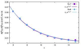
Figure 1: Analysis details to study scaling dimension of the scalar using the difference between the zero spatial momentum correlator and the point-to-point correlator of the scalar meson using overlap fermion with $m_{w}=1.0$. The left panel shows sample behavior of $R_{S}^{p}(x,L)-R_{S}^{z}(x,L)-\frac{2}{3\pi^{2}}$ as a function of $\left(\frac{x}{L}\right)^{2}$ and the associated two different fits. The value of $R_{S}^{p}(x)-R_{S}^{z}(x)-\frac{2}{3\pi^{2}}$ that is extracted for all values of $x\in[6,15]$ are shown along with the extrapolation errors in the right panel. The limit as $x\to\infty$, using single exponential fits of the type $c_{1}e^{-c_{2}x}$ shown as curves in the right panel, is consistent with zero.

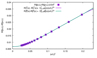
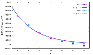
Figure 2: Analysis details to study the absence of perturbative corrections to the scaling dimension of the vector using the difference of the zero spatial momentum correlator and the point-to-point correlator of the vector meson obtained using overlap fermion with $m_{w}=1.0$. The left panel shows a sample behavior of $R_{V}^{p}(x,L)-R_{V}^{z}(x,L)$ as a function of $\left(\frac{x}{L}\right)^{2}$ at $x=8$ and the associated fits with two different orders $N$. The value of $R_{S}^{p}(x)-R_{S}^{z}(x)$ so extracted for all values of $x\in[8,14]$ are shown along with the extrapolation errors in the right panel. The limit as $x\to\infty$ using single exponential fit, as for the scalar case above, is consistent with zero.

We first concentrate on the scaling dimensions of scalar and the vector within the lattice perturbation theory at ${\cal O}(q^{2})$, and can be obtained from $R_{S}$ and $R_{V}$ is the above equations. For the isotriplet vector, one expects there to be no corrections from interaction to its free field scaling dimension. The combinations,

$$R_{S}^{p}(x)-R_{S}^{z}(x)\sim\gamma_{S}^{1}q^{2};\qquad R_{V}^{p}(x)-R_{V}^{z}(x)\sim 0,$$ (74)

for $|x|\gg 1$, can be seen to be good observables to extract the ${\cal O}(q^{2})$ corrections to the scaling dimensions.

We study the above quantity for the scalar correlator using overlap fermion with $m_{w}=1.0$ in Figure 1. From the dimensional regulatization computation, it is known that $\gamma_{S}^{1}=\frac{2}{3\pi^{2}}$. Therefore, we consider the combination $R_{S}^{p}(x,L)-R_{S}^{z}(x,L)-\frac{2}{3\pi^{2}}$. The left panel shows its behavior as a function of $\left(\frac{x}{L}\right)^{2}$ for a sample case of $x=8$. The infinite volume limits at each each fixed $x$ were obtained using the Ansatz of the type in Eq. (73). Such infinite volume extrapolated values at each $x$ with $N=7,8$ are plotted in the right panel as a function of $x$. It can be seen that the limit $x\to\infty$ is consistent with zero and a single exponential fit, $c_{1}e^{-c_{2}x}$, matches the data reasonably well. Thus, we have shown that the result of $\gamma_{S}^{1}$ for the lattice model agrees with the expectation from dimensional regularization in the continuum at ${\cal O}(q^{2})$. In addition to such a universality between continuum and lattice regulators, we also checked that the results for $\gamma_{S}^{1}$ from different $m_{w}$ in overlap fermion agree.

For the vector operator, we expect its scaling dimension to be uncorrected from the free field value to all orders in $q^{2}$. We demonstrate this using a similar strategy as for the scalar as shown in Figure 2. The left panel shows the behavior of $R_{V}^{p}(x,L)-R_{V}^{z}(x,L)$ as a function of $\left(\frac{x}{L}\right)^{2}$ for $x=8$. The infinite volume extrapolated values at each $x$ with $N=7,8$ are plotted in the right panel as a function of $x$. Again, we find the limit $x\to\infty$ is consistent with zero and a single exponential fit matches the data reasonably well. The estimated value at $x=14$ from $N=7$ and $N=8$ fall on either side of zero. This implies that Eq. (74) for the vector is reproduced without any regulator dependence.

IV.2 Two-point function amplitudes

IV.2.1 Regulator dependence

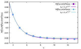
Figure 3: Analysis details to obtain the scalar two-point function amplitude using overlap fermion with $m_{w}=0.5$. The left panel shows sample behavior of $R_{S}^{p}(x,L)$ as a function of $\left(\frac{x}{L}\right)^{2}$ and the associated two different fits of the type in Eq. (73) with $N=7$ and 8. The value of $R_{S}^{p}(x)-\frac{4}{3\pi^{2}}\ln(x)$ so extracted for all values of $x\in[4,13]$ are shown along with the extrapolation errors in the right panel. The single exponential fits to extract the amplitude in $x\to\infty$ limit are also shown as the curves.

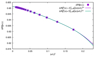
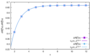
Figure 4: A comparison of the results for overlap fermions with $m_{w}=0.5$ and $m_{w}=1.0$. The left panel shows a sample behavior of $\Delta R_{S}^{p}(x,L)$ as a function of $\left(\frac{x}{L}\right)^{2}$ and the associated two different fits. The value of $\Delta R_{S}^{p}(x)$ so extracted for all values of $x\in[2,12]$ are shown along with the errors in the right panel. The limit as $x\to\infty$ is not zero and finite showing that the amplitude of the two-point function depends on the regulator parameter.

We start our analysis by focussing on overlap fermion with $m_{w}=0.5$. The details are shown in Figure 3. The left panel shows the data for $R_{S}^{p}(x,L)$ for overlap fermion with $m_{w}=0.5$. The data is plotted as a function of $\left(\frac{x}{L}\right)^{2}$ for a sample case of $x=6$. The extrapolated values at $L=\infty$ are $R_{S}^{p7}(6)=-0.66913$ and $R_{S}^{p8}(6)=-0.66903$ and there is only a small systematic change in the fit values when one goes from $N=7$ to $N=8$. Assuming that $\gamma_{S}^{1}=\frac{2}{3\pi^{2}}$, we plot $R_{S}^{p}(x)-\frac{4}{3\pi^{2}}\ln x$ in the right panel for $N=7,8$ using the infinite volume extrapolated values at different $x$. We see that the limit as $x\to\infty$ is finite and non-zero. A fit with a constant and single exponential fits the data well and we find that

$$\frac{C_{S}^{1}}{C_{S}^{0}}\Bigg{|}_{m_{w}=0.5}=-0.9885(6),$$ (75)

by comparing with Eq. (71). The error in the numerical value on the right hand side of the above equation comes from the difference in the $N=7$ and $N=8$ values.

Next, we investigate the regulator dependence of the amplitude. To this end, we vary the Wilson mass parameter, $m_{w}$, within overlap fermions. If the result is independent of the regulator, the difference in the results for two different choices of $m_{w}$ should go to zero as $x\to\infty$. Let,

$$\Delta R_{S}^{p}(x,L)=R_{S}^{p}(x,L;m_{w})-R_{S}^{p}(x,L;m_{w}=0.5),$$ (76)

denote the difference between two different regulators. Comparison of overlap fermion with $m_{w}=1.0$ to overlap fermion with $m_{w}=0.5$ is analyzed in Figure 4. The right panel shows the data for $\Delta R_{S}^{p}(x,L)$ where the difference is obtained by subtracting the ratio for overlap fermion with $m_{w}=0.5$ from overlap fermion with $m_{w}=1.0$. The data is plotted as a function of $\left(\frac{x}{L}\right)^{2}$ for $x=5$. A fit of the form in Eq. (73) with $N=4$ and $N=5$ are also shown. The extrapolated values at $L=\infty$ are $\Delta R_{S}^{p4}(5)=0.651420$ and $\Delta R_{S}^{p5}(5)=0.651440$, thereby showing only a small systematic dependence on the extrapolation ansatz. The systematic change in the fit values between the two choices of extrapolations is small. The extrapolated values, $\Delta R_{S}^{p4}(x)$ and $\Delta R_{S}^{p5}(x)$, are plotted as a function of $x\in[2,12]$ in the right panel. The $x\to\infty$ limit is approached exponentially and the data is fit using a constant and a single exponential. The limits are non-zero and finite, which clearly shows that the amplitude depends on the regulator parameter. The dependence of the amplitude on $m_{w}$ are shown in the second column of Table 1.

$m_{w}$	$\frac{C_{S}^{1}}{C_{S}^{0}}\Bigg{|}_{m_{w}}-\frac{C_{S}^{1}}{C_{S}^{0}}\Bigg{|}_{0.5}$	Tadpole corrected result
0.25	-1.3328(37)	-0.1390(37)
0.75	0.44590(10)	0.04797(10)
1.0	0.66976(6)	0.07286(6)
1.25	0.80593(9)	0.08965(9)
1.5	0.89843(43)	0.10256(43)
1.75	0.9678(18)	0.1151(18)

Table 1: Table showing the dependence of the scalar meson amplitude ratio on the regulator for overlap fermions. The second column is using the unimproved gauge links, and the third column is using tadpole improved gauge links (see text).

Our analysis of vector mesons mirrors the one for scalar mesons. We start our analysis by focusing on overlap fermion with $m_{w}=0.5$ to extract the amplitude. The details are shown in Figure 5. The left panel shows the data for $R_{V}^{p}(x,L)$ for overlap fermion with $m_{w}=0.5$. The data is plotted as a function of $\left(\frac{x}{L}\right)^{2}$ for $x=6$. We needed to use $N=7$ and $N=8$ in Eq. (73) (the form of fit is same for vector and scalar mesons) to best fit the data and these are also shown. The extrapolated values at $L=\infty$ are $R_{S}^{p7}(6)=-0.910487$ and $R_{S}^{p7}(6)=-0.910450$. We plot $R_{V}^{p}(x)$ in the right panel for $N=7,8$. We see that the limit as $x\to\infty$ is finite and non-zero. A fit with a constant and single exponential fits the data well and we find that

$$\frac{C_{V}^{1}}{C_{V}^{0}}\Bigg{|}_{m_{w}=0.5}=-0.92254(13).$$ (77)

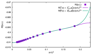
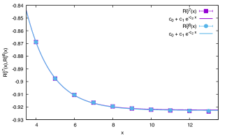
Figure 5: Analysis details for the zero spatial momentum projected vector correlator using overlap fermion with $m_{w}=0.5$. The left panel shows sample behavior of $R_{V}^{p}(x,L)$as a function of $\left(\frac{x}{L}\right)^{2}$ at a sample $x=5$, and the associated two different infinite volume extrapolation fits. The value of $R_{V}^{p}(x)$ so extracted for all values of $x\in[4,13]$ are shown along with the errors in the right panel. The fits to extract the leading correction to the amplitude are also shown.

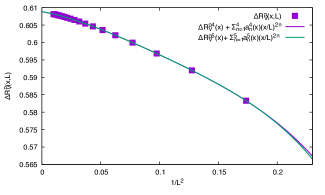
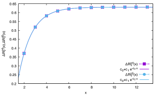
Figure 6: A comparison of the results for overlap fermions with $m_{w}=0.5$ and $m_{w}=1.0$. The left panel shows a sample behavior of $\Delta R_{V}^{p}(x,L)$ as a function of $\left(\frac{x}{L}\right)^{2}$ and the associated two different fits. The value of $\Delta R_{V}^{p}(x)$ so extracted for all values of $x\in[2,12]$ are shown along with the errors in the right panel. The limit as $x\to\infty$ is not zero and finite showing that the amplitude of the two-point function depends on the regulator parameter.

Like in the case of scalar mesons, we investigate the regulator dependence of the amplitude by varying the Wilson mass parameter, $m_{w}$, within overlap fermions. Comparison of overlap fermion with $m_{w}=1.0$ to overlap fermion with $m_{w}=0.5$ is analyzed in Figure 6. The right panel shows the data for $\Delta R_{V}^{p}(x,L)$ where the difference is obtained by subtracting the ratio for overlap fermion with $m_{w}=0.5$ from overlap fermion with $m_{w}=1.0$. The data is plotted as a function of $\left(\frac{x}{L}\right)^{2}$ for $x=5$. A fit of the form in Eq. (73) with $N=4$ and $N=5$ are also shown. The extrapolated values at $L=\infty$ are $\Delta R_{V}^{p4}(5)=0.608857$ and $\Delta R_{V}^{p5}(5)=0.608873$. We see only a small systematic change in the fit values when one goes from $N=4$ to $N=5$. The extrapolated values, $\Delta R_{V}^{p4}(x)$ and $\Delta R_{V}^{p5}(x)$, are plotted as a function of $x\in[2,13]$ in the right panel. The $x\to\infty$ limit is approached exponentially and the data is fit using a constant and a single exponential. The limits are non-zero and finite clearly showing that the amplitude of vector two-point function also depends on the regulator parameter. The dependence of the amplitude on $m_{w}$ are shown in the second column of Table 2.

IV.2.2 Partial restoration of universality with tadpole improvement

The regulator dependence of the two-point functions seen in Table 1 and Table 2 in the lattice model is a curious aspect of this lattice gauge model, which approaches the continuum behavior simply at distance scales much larger than one lattice unit without any fine tuning. The regulator dependence of amplitudes is to be understood by the fact that the plaquette value in this model never approaches 1 due to the absence of the traditional continuum limit at a field field fixed point. Thus, we wanted to check whether by “improving” the Dirac operator by using gauge links that are closer to unity subdues the regulator dependence of the amplitudes. A well known method to achieve this is via tadpole improvement, namely, the replacement of the massless free Wilson-Dirac operator in Eq. (18) by

$$D_{0}(x_{1},x_{2})=3\delta_{x_{2},x_{1}}-u_{o}\sum_{i}\left[p_{i+}\delta_{x_{2},x_{1}+\hat{i}}+p_{i-}\delta_{x_{2},x_{1}-\hat{i}}\right]$$ (78)

where $u_{0}^{4}$ is the expectation value of the compact plaquette with charge $q$. A simple computation yields,

$$u_{0}=\exp\left[-\frac{q^{2}}{24L^{3}}\sum^{\prime}_{p}\Box(p)\right]=e^{-\alpha q^{2}};\qquad\alpha=0.0994834.$$ (79)

This amounts to a change in the Wilson mass parameter by

$$m_{w}\to\frac{m_{w}-3(1-u_{0})}{u_{0}}.$$ (80)

Since the free massless overlap propagator behaves as

$$\tilde{G}_{e}(q)=2m_{w}\frac{i\sigma_{k}p_{k}}{p^{2}};\qquad p_{k}=\frac{2\pi q_{k}}{L}\to 0$$ (81)

the induced wavefunction normalization is $\frac{1}{2m_{w}}$ for each fermion propagator. Since $m_{w}$ has a tadpole correction given by Eq. (80), we conclude that all ratios defined in Eq. (71) should be multiplied by

$$\left[\frac{u_{0}}{1-\frac{3(1-u_{0})}{m_{w}}}\right]^{2}=\left[1+\frac{2(3-m_{w})\alpha}{m_{w}}q^{2}+\cdots\right].$$ (82)

This amounts to

$$\frac{C_{S,V}^{1}}{C_{S,V}^{0}}\to\frac{C_{S,V}^{1}}{C_{S,V}^{0}}+\frac{2(3-m_{w})\alpha}{m_{w}}$$ (83)

resulting in

$$\frac{C_{S}^{1}}{C_{S}^{0}}\Bigg{|}_{m_{w}=0.5}+10\alpha=0.0063(6),$$ (84)

as the tadpole corrected amplitude ratio at $m_{w}=0.5$ and

$$\frac{C_{S}^{1}}{C_{S}^{0}}\Bigg{|}_{m_{w}}-\frac{C_{S}^{1}}{C_{S}^{0}}\Bigg{|}_{m_{w}=0.5}+\frac{6(1-2m_{w})\alpha}{m_{w}}$$ (85)

as the tadpole corrected difference of the amplitude ratio. These are shown in the third column of Table 1. Since the logic of the tadpole correction carries over to vector mesons, we can use Eq. (85) to include a tadpole correction resulting in

$$\frac{C_{V}^{1}}{C_{V}^{0}}\Bigg{|}_{m_{w}=0.5}+10\alpha=0.07229(13),$$ (86)

and the third column in Table 2. In both the scalar and vector cases, the regulator dependence in the tadpole improved case is indeed weaker.

$m_{w}$	$\frac{C_{V}^{1}}{C_{V}^{0}}\Bigg{|}_{m_{w}}-\frac{C_{V}^{1}}{C_{V}^{0}}\Bigg{|}_{0.5}$	Tadpole corrected result
0.25	-1.3072(44)	-0.1134(44)
0.75	0.42461(7)	0.02668(7)
1.0	0.630541(7)	0.033641(6)
1.25	0.75052(7)	0.03424(7)
1.5	0.8276(6)	0.0317(6)
1.75	0.8824(18)	0.0297(18)

Table 2: Table showing the dependence of the vector meson amplitude ratio on the regulator for overlap fermions. The second column is using the unimproved gauge links, and the third column is using tadpole improved gauge links (see text).

V Conclusions

It is useful to compute corrections to conformal correlation functions in a perturbation theory that maintains conformal invariance Chester and Pufu (2016); Giombi et al. (2016), with the possibility of performing $N$-point functions beyond $N=2$ on larger lattices without a Monte Carlo effort. Naively, only the anomalous scaling dimensions of operators and amplitudes of three point functions and higher (with the amplitudes of 2-point function set to unity as the normalization condition) are physical. There are situations that involve conserved operators where the amplitude of two point functions become physical. One such quantity is the vector current in conformal three dimensional QED. A lattice model to reproduce results in conformal three dimensional QED was proposed in Karthik and Narayanan (2020). We studied this model using lattice perturbation theory in this paper. We computed corrections to the scalar and vector two point functions. We showed that the scalar anomalous dimension is correctly reproduced and is independent of the regulator, thereby validating further future efforts within a lattice perturbation theory setup. On the other hand, we showed that the corrections to the amplitude of the scalar and vector two point function depends on the lattice regulator. In particular, we found that the amplitude of the vector correlator depends on the lattice regulator. This observation demands one to numerically revisit the verification Karthik and Narayanan (2020) of the conjectured self-duality of three dimensional QED with four flavors of two component fermions Wang et al. (2017); Xu and You (2015); Hsin and Seiberg (2016) within the framework of the lattice conformal model via the degeneracy of flavor current and topological current correlators; in the work Karthik and Narayanan (2020), the regulator dependence was not explored. Since such a degeneracy between the correlators was also seen to arise within statistical errors in a conventional simulation of three dimensional QED Karthik and Narayanan (2017) with a well-defined continuum limit, we suspect that the value of $q$ in the lattice model where the flavor and vector currents coincide might turn out to be a universal value independent of the regulator. For this, one might need to use the induced Chern-Simons terms from massive fermions to compute the topological current correlator, wherein similar regulator dependence could be induced in the correlators of the fermion-based definition of the topological currents as well. Such a scenario conjectured by us needs to be studied further. In the future, it would also be interested to use the model to study scaling dimensions of monopoles by coupling the lattice model to the gauge field $qA+{\cal A}_{Q}$, with $A$ being the dynamical gauge field and ${\cal A}_{Q}$ being the background gauge field for a flux $Q$ monopole-antimonopole pair as studied in Karthik and Narayanan (2019); Karthik (2018), and ask if they match the values found in different $N_{f}$ flavor QED₃.