$\mathcal{PT}$-symmetric $-g\varphi^{4}$ theory

Abstract

The scalar field theory with potential $V(\varphi)=\textstyle{\frac{1}{2}}m^{2}\varphi^{2}-\textstyle{\frac{1}{4}}g\varphi^{4}$ ($g>0$) is ill defined as a Hermitian theory but in a non-Hermitian $\mathcal{P}\mathcal{T}$-symmetric framework it is well defined, and it has a positive real energy spectrum for the case of spacetime dimension $D=1$. While the methods used in the literature do not easily generalize to quantum field theory, in this paper the path-integral representation of a $\mathcal{P}\mathcal{T}$-symmetric $-g\varphi^{4}$ theory is shown to provide a unified formulation for general $D$. A new conjectural relation between the Euclidean partition functions $Z^{\mathcal{P}\mathcal{T}}(g)$ of the non-Hermitian $\mathcal{P}\mathcal{T}$-symmetric theory and $Z_{\rm Herm}(\lambda)$ of the $\lambda\varphi^{4}$ ($\lambda>0$) Hermitian theory is proposed: $\log Z^{\mathcal{P}\mathcal{T}}(g)=\textstyle{\frac{1}{2}}\log Z_{\rm Herm}(-g+{\rm i}0^{+})+\textstyle{\frac{1}{2}}\log Z_{\rm Herm}(-g-{\rm i}0^{+})$. This relation ensures a real energy spectrum for the non-Hermitian $\mathcal{P}\mathcal{T}$-symmetric $-g\varphi^{4}$ field theory. A closely related relation is rigorously valid in $D=0$. For $D=1$, using a semiclassical evaluation of $Z^{\mathcal{P}\mathcal{T}}(g)$, this relation is verified by comparing the imaginary parts of the ground-state energy $E_{0}^{\mathcal{P}\mathcal{T}}(g)$ (before cancellation) and $E_{0,\rm Herm}(-g\pm{\rm i}0^{+})$.

I Introduction

In search of physics beyond the Standard Model of particle physics, non-Hermitian $\mathcal{PT}$-symmetric Hamiltonians have been used recently in model building R01 . The importance of $\mathcal{PT}$ symmetry for non-Hermitian quantum-mechanical theories with real energy eigenvalues was discovered in 1998 R02 on the basis of numerical and semiclassical arguments. The quantum-mechanical theories considered are governed by a Schrödinger equation with potential $V(x)=m^{2}x^{2}/2+gx^{2}(\mathrm{i}x)^{\epsilon}/4$, where $\epsilon$ is a real parameter. This potential is invariant under $\mathcal{PT}$ reflection $\mathcal{P}:\ x\to-x,\ \mathcal{T}:\ x\to x,\ \mathrm{i}\to-\mathrm{i}$. For $\epsilon\geq 0$ the energy spectrum of the Hamiltonian was found to be real numerically R02 . For the massless case spectral reality was proved for $\epsilon>0$ by Dorey et al. using the methods of integrable systems R03 ; R04 . For $\epsilon=2$ the massless case can be mapped to a Hermitian Hamiltonian with the same spectrum R05 ; R06 . The study of $\mathcal{PT}$-symmetric systems is an active research area R04 ; R07 .

Quantum mechanics is quantum field theory in one-dimensional spacetime. However, very little is known about the nature of $\mathcal{PT}$-symmetric quantum field theory with spacetime dimension $D>1$, and the calculational tools required for analyzing such theories remain largely undeveloped. Methods that have been successful in $D=1$ R04 do not extend to higher dimensions. Recent papers R08 ; R09 ; R010 have considered the case $D>1$, but the proposed methods have yet to be implemented in $D=4$.

In this paper we study the non-Hermitian $\mathcal{PT}$-symmetric scalar theory with potential $V(\varphi)=m^{2}\varphi^{2}/2-g\varphi^{4}/4$ ($m,\,g>0$) using the path-integral formulation of quantum theories. Unlike earlier methods, here we study this theory by constructing a relation between its Euclidean partition function and that of a Hermitian theory with a positive quartic potential $V(\phi)=m^{2}\varphi^{2}/2+\lambda\varphi^{4}/4$ ($m,\,\lambda>0$). Specifically, we conjecture and propose the following general relation for $D\geq 1$:

$$\log Z^{\mathcal{P}\mathcal{T}}(g) = \textstyle{\frac{1}{2}}\log Z_{\rm Herm}(\lambda=-g+\mathrm{i}0^{+})$$ (1)

$$\quad+\textstyle{\frac{1}{2}}\log Z_{\rm Herm}(\lambda=-g-\mathrm{i}0^{+}),$$

where $Z_{\rm Herm}(\lambda)$ is the usual Euclidean partition function for the Hermitian theory, which must be analytically continued to $\lambda=-g\pm\mathrm{i}0^{+}$ ($g>0$) in this equation. The functional integral $Z^{\mathcal{P}\mathcal{T}}(g)$ must be defined with an appropriate contour $\mathcal{C}_{\mathcal{P}\mathcal{T}}$ to ensure both existence and $\mathcal{PT}$ symmetry, as will be explained. The Euclidean partition function can always be put in a form of an exponential function via the exponentiation of disconnected Feynman diagrams in perturbation theory or of the multi-instanton contributions when there are nonpeturbative stationary points; $\log Z$ is related to the energy. Therefore, (1) implies that

$$\!E^{\mathcal{P}\mathcal{T}}(g)=\textstyle{\frac{1}{2}}E_{\rm Herm}(-g+\mathrm{i}0^{+})+\textstyle{\frac{1}{2}}E_{\rm Herm}(-g-\mathrm{i}0^{+}).$$ (2)

For positive real $\lambda$, $E_{\rm Herm}(\lambda)=E^{*}_{\rm Herm}(\lambda^{*})$. This relation is analytic, so it holds when $E_{\rm Herm}(\lambda)$ is analytically continued to $\lambda=-g+\mathrm{i}0^{+}$. We thus have ${\rm Re}[E_{\rm Herm}(-g+\mathrm{i}0^{+})]={\rm Re}[E_{\rm Herm}(-g-\mathrm{i}0^{+})]$ and ${\rm Im}[E_{\rm Herm}(-g+\mathrm{i}0^{+})]=-{\rm Im}[E_{\rm Herm}(-g-\mathrm{i}0^{+})]$. Therefore, (1) implies a real energy spectrum for the non-Hermitian $-g\varphi^{4}$ theory.

We first study an analogous relation for toy $D=0$ partition functions, which are ordinary integrals. The relation in this case takes a form similar to (1) but without logarithms, and it can be rigorously proved because the toy partition functions can be calculated exactly. We then discuss some simple generalizations in $D=0$ in order to understand why the logarithms in (1) appear when one considers partition functions with $D\geq 1$, which are functional integrals. For $D=1$, we partly check the relation by calculating the imaginary contributions to the ground-state energy. Although on both sides of (2) the imaginary parts cancel trivially, before their cancellation one can find agreement between separate pieces on the LHS and RHS. Since in the path-integral formulation, there is no essential difference between the cases $D>1$ and $D=1$ except for the well-understood regularisation and renormalization, we conjecture that the relation (1) holds also for $D>1$.

II Case $D=0$

II.1 Full results

The toy $D=0$ model has been studied earlier in R04 ; R011 and is a good platform to illustrate the idea. We first consider the Hermitian partition function

$$\widetilde{Z}_{\rm Herm}(\lambda)=\int_{-\infty}^{\infty}{\rm d}x\,\exp\left(-\textstyle{\frac{1}{2}}{m^{2}x^{2}}-\textstyle{\frac{1}{4}}\lambda x^{4}\right),$$ (3)

where $\lambda>0$. When $\lambda=-g<0$, the integral above is divergent, but we can consider the $\mathcal{PT}$-symmetric non-Hermitian theory,

$$\widetilde{Z}^{\mathcal{P}\mathcal{T}}(g)=\lim_{\epsilon\rightarrow 2}\int_{\mathcal{C}_{\mathcal{P}\mathcal{T}}}\mathrm{d}x\,\exp\left(-\textstyle{\frac{1}{2}}m^{2}x^{2}-\textstyle{\frac{1}{4}}gx^{2}(\mathrm{i}x)^{\epsilon}\right),$$ (4)

where for $\epsilon=2$, $\mathcal{C}_{\mathcal{P}\mathcal{T}}$ is a continuous contour that terminates in the $\mathcal{PT}$-symmetric Stokes wedges $-\frac{3}{8}\pi<\arg x<-\frac{1}{8}\pi$ and $-\frac{7}{8}\pi<\arg x<-\frac{5}{8}\pi$. The contour $\mathcal{C}_{\mathcal{P}\mathcal{T}}$ is not unique; deforming a contour joining the $\mathcal{PT}$-symmetric Stokes wedges leaves the value of the integral unchanged. An example of $\mathcal{C}_{\mathcal{P}\mathcal{T}}$ is shown as the solid line in Fig. 1. Below, we show that the above toy partition functions satisfy

$$\widetilde{Z}^{\mathcal{P}\mathcal{T}}(g)=\textstyle{\frac{1}{2}}\widetilde{Z}_{\rm Herm}(-g+\mathrm{i}0^{+})+\textstyle{\frac{1}{2}}\widetilde{Z}_{\rm Herm}(-g-\mathrm{i}0^{+}).$$ (5)

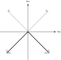
Figure 1: An example of the contour $\mathcal{C}_{\mathcal{P}\mathcal{T}}$ is shown as the solid line. Also shown are two other contours (dashed lines) $\mathcal{C}_{1}:\mathrm{e}^{-\mathrm{i}\pi/4}(-\infty,+\infty)$, and $\mathcal{C}_{2}:\mathrm{e}^{\mathrm{i}\pi/4}(-\infty,+\infty)$.

Using the contour $C_{\mathcal{P}\mathcal{T}}$ shown in Fig. 1 for (4) we get

$$\widetilde{Z}^{\mathcal{P}\mathcal{T}}(g)=\mathrm{e}^{\mathrm{i}\pi/4}\int_{-\infty}^{0}\mathrm{d}x\,\exp\left(-\textstyle{\frac{1}{2}}\mathrm{i}m^{2}x^{2}-\textstyle{\frac{1}{4}}gx^{4}\right)$$

$$\qquad\qquad\,+\mathrm{e}^{-\mathrm{i}\pi/4}\int^{\infty}_{0}\mathrm{d}x\,\exp\left(\textstyle{\frac{1}{2}}\mathrm{i}m^{2}x^{2}-\textstyle{\frac{1}{4}}gx^{4}\right)$$

$$=\frac{m\pi}{2\sqrt{2g}}\exp\left(-\frac{m^{4}}{8g}\right)\left[I_{-\frac{1}{4}}\left(\frac{m^{4}}{8g}\right)+I_{\frac{1}{4}}\left(\frac{m^{4}}{8g}\right)\right],$$ (6)

where $I_{\pm\frac{1}{4}}(z)$ is the modified Bessel function of the first kind. On the other hand, doing the integral in (3) gives $\widetilde{Z}_{\rm Herm}(\lambda)=\frac{m}{\sqrt{2\lambda}}\exp\left(\frac{m^{4}}{8\lambda}\right)K_{\frac{1}{4}}\left(\frac{m^{4}}{8\lambda}\right)$, where $K_{\frac{1}{4}}(z)$ is the modified Bessel function of the second kind. $K_{\frac{1}{4}}(z)$ has a branch cut on the negative axis and for $z>0$

$$K_{\frac{1}{4}}(-z\pm\mathrm{i}0^{+})= \frac{\pi}{2}\left(I_{-\frac{1}{4}}(z)-I_{\frac{1}{4}}(z)\right)$$

$$\mp\frac{\mathrm{i}\pi}{2}\left(I_{-\frac{1}{4}}(z)+I_{\frac{1}{4}}(z)\right).$$ (7)

Substituting the above equation into $\textstyle{\frac{1}{2}}Z_{\rm Herm}(-g+\mathrm{i}0^{+})+\textstyle{\frac{1}{2}}Z_{\rm Herm}(-g-\mathrm{i}0^{+})$, we obtain the result in (II.1), which proves the relation (5).

One may understand the relation (5) in another way. When the function $\widetilde{Z}_{\rm Herm}(\lambda)$ is analytically continued away from the positive real axis via $\lambda=g\exp(\mathrm{i}\theta)$, where $g>0$, it could still have an integral representation as in (3) but with the contour rotated via $x\to x\exp(-\mathrm{i}\theta/4)$. Then, $\widetilde{Z}_{\rm Herm}(g\mathrm{e}^{\mathrm{i}(\pi-0^{+})})$ could be represented by the same integral but with the contour given by $\mathcal{C}_{1}$ in Fig. 1, while $\widetilde{Z}_{\rm Herm}(g\mathrm{e}^{-\mathrm{i}(\pi-0^{+})})$ corresponds to the contour $\mathcal{C}_{2}$. In these cases, the integrand is the same as that in (4) with $\epsilon=2$. Because of the symmetry $x\to-x$ in the integrand, the contour $\mathcal{C}_{\mathcal{P}\mathcal{T}}$ can be effectively viewed as half $\mathcal{C}_{1}$ plus half $\mathcal{C}_{2}$ and thus one arrives at the relation (5).

II.2 Imaginary parts and semi-classical estimates

In the above example the partition functions can be calculated exactly. This is not possible when $D\geq 1$. Therefore, we search for an alternative approach where precise results of the partition functions are not needed, but one still can examine the relation between the Hermitian and the non-Hermitian $\mathcal{PT}$-symmetric Euclidean partition functions. From (II.1), one sees that $\widetilde{Z}_{\rm Herm}(-g\pm\mathrm{i}0^{+})$ contains an imaginary part:

$${\rm Im}\left[\widetilde{Z}_{\rm Herm}(-g\pm\mathrm{i}0^{+})\right]$$

$$=\pm\frac{m\pi}{2\sqrt{2g}}\exp\left(-\frac{m^{4}}{8g}\right)\left[I_{\frac{1}{4}}\left(\frac{m^{4}}{8g}\right)-I_{-\frac{1}{4}}\left(\frac{m^{4}}{8g}\right)\right]$$

$$=\mp\frac{\sqrt{\pi}}{m}\mathrm{e}^{-m^{4}/4g}{\rm\ for\ }g\to 0.$$ (8)

Although these imaginary parts cancel trivially on the RHS of (5), one can still observe the same imaginary parts on the LHS in evaluating $\widetilde{Z}^{\mathcal{P}\mathcal{T}}(g)$ semiclassically.

For small $g$ we approximate the integral (4) using the method of steepest descents R012 . There are three stationary points: $x_{\rm L}=-m/\sqrt{g}$, $x_{0}=0$, and $x_{\rm R}=m/\sqrt{g}$. Steepest paths satisfy the constant-phase condition ${\rm Im}\left[m^{2}x^{2}/2-gx^{4}/4\right]={\rm const}$, where the constant is determined by the phase at the stationary point. Writing $x=x_{\rm Re}+\mathrm{i}x_{\rm Im}$, we have $m^{2}(x_{\rm Re}x_{\rm Im})=g(x_{\rm Re}x_{\rm Im})(x^{2}_{\rm Re}-x^{2}_{\rm Im})$, which gives $x_{\rm Re}=0,\,x_{\rm Im}=0,\,x^{2}_{\rm Re}-x^{2}_{\rm Im}=m^{2}/g$. At the stationary point $x_{0}$, the solution with $x_{\rm Im}=0$ corresponds to the steepest-descent path, while at $x_{\rm L}$ or $x_{\rm R}$, $x^{2}_{\rm Re}-x^{2}_{\rm Im}=m^{2}/g$ gives the steepest-descent path.

Next, we deform the contour $\mathcal{C}_{\mathcal{P}\mathcal{T}}$ to the new one $\mathcal{C}^{\prime}_{\mathcal{P}\mathcal{T}}$ shown in Fig. 2. In the case of a path integral for $D\geq 1$, all the steepest-descent paths crossing a stationary point constitute a hypersurface called a Lefschetz thimble R013 ; R014 ; R015 ; R016 . For $D=0$, Lefschetz thimbles reduce to the steepest-descent one-dimensional paths through the stationary points, e.g., the hyperbolas in Fig. 2. Anticipating the generalisation of our analysis to the case $D=1$, we call these paths in the present case thimbles, which are denoted by $\mathcal{J}_{\rm L}$, $\mathcal{J}_{0}$, and $\mathcal{J}_{\rm R}$. We denote the half Lefschetz thimble of $\mathcal{J}_{\rm L}$ that goes to the lower (upper) half plane as $\mathcal{J}_{\rm L,-(+)}$. Similarly, we denote the half Lefschetz thimble of $\mathcal{J}_{\rm R}$ going to the lower (upper) half plane as $\mathcal{J}_{\rm R,-(+)}$. Thus, the deformed contour can be expressed as $\mathcal{C}^{\prime}_{\mathcal{P}\mathcal{T}}=\mathcal{J}_{\rm L,-}+\mathcal{J}_{0}+\mathcal{J}_{\rm R,-}$, which is left-right symmetric. The leading contribution to $\rm{Im}[\widetilde{Z}^{\mathcal{P}\mathcal{T}}(g)]$ is easily obtained by evaluating the integral on $\mathcal{J}_{\rm L,-}$ and $\mathcal{J}_{\rm R,-}$ up to the Gaussian fluctuations:

$${\rm Im}\left[\left.\widetilde{Z}^{\mathcal{P}\mathcal{T}}(g)\right|_{\mathcal{J}_{\rm L/R,-}}\right]=\pm\frac{\sqrt{\pi}}{2m}\exp(-m^{4}/(4g)).$$

These imaginary parts differ by a sign and so they also cancel on the LHS of (5). Comparing the above equation with the last line in (II.2), we see that for small $g$ the imaginary parts from $\mathcal{J}_{\rm L,-}$ and $\mathcal{J}_{\rm R,-}$ are equal to those from $\textstyle{\frac{1}{2}}\widetilde{Z}_{\rm Herm}(-g-\mathrm{i}0^{+})$ and $\textstyle{\frac{1}{2}}\widetilde{Z}_{\rm Herm}(-g+\mathrm{i}0^{+})$. The imaginary part from $\mathcal{J}_{\rm L,-}$ is supposed to be that from the left part of the standard contour $\mathcal{C}_{\mathcal{P}\mathcal{T}}$ which is also the left part of $\mathcal{C}_{2}$ (see Fig. 1). The integral on the latter gives half of $Z_{\rm Herm}(-g-\mathrm{i}0^{+})$. This explains the correspondence $\mathcal{J}_{\rm L,-}\leftrightarrow-g-\mathrm{i}0^{+};\,\mathcal{J}_{\rm R,-}\leftrightarrow-g+\mathrm{i}0^{+}$ in comparing the imaginary parts from the LHS and RHS of (5).

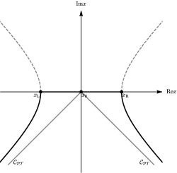
Figure 2: The deformed contour $\mathcal{C}^{\prime}_{\mathcal{P}\mathcal{T}}$ (heavy solid line) is composed of steepest-descent paths through the stationary points $x_{\rm L}$ (left half-hyperboloid), $x_{0}$ (the real line), and $x_{\rm R}$ (right half-hyperboloid).

II.3 Simple generalizations

The relation (5) is not general. To see why, consider a generalization of the partition functions in (3) and (4). One can consider $Z_{\rm Herm}(\lambda)=[\widetilde{Z}_{\rm Herm}(\lambda)]^{2}$. This partition function would be given by a double integral with the integrand being the product of that in (3) for each variable. The corresponding non-Hermitian partition function would be given as $Z^{\mathcal{P}\mathcal{T}}(g)=[\widetilde{Z}^{\mathcal{P}\mathcal{T}}(g)]^{2}$. These partition functions do not satisfy $Z^{\mathcal{P}\mathcal{T}}(g)=Z_{\rm Herm}(-g+\mathrm{i}0^{+})/2+Z_{\rm Herm}(-g-\mathrm{i}0^{+})/2$ but rather $\sqrt{Z^{\mathcal{P}\mathcal{T}}(g)}=\sqrt{Z_{\rm Herm}(-g+\mathrm{i}0^{+})}/2+\sqrt{Z_{\rm Herm}(-g-\mathrm{i}0^{+})}/2$. One can also consider $Z_{\rm Herm}(\lambda)=\exp[\widetilde{Z}_{\rm Herm}(\lambda)]$ and $Z^{\mathcal{P}\mathcal{T}}(g)=\exp[\widetilde{Z}^{\mathcal{P}\mathcal{T}}(g)]$, which satisfy (1) rather than (5).

In these examples $\widetilde{Z}^{\mathcal{P}\mathcal{T}}$ and $\widetilde{Z}_{\rm Herm}$ are the fundamental ingredients in the partition functions $Z^{\mathcal{P}\mathcal{T}}$ and $Z_{\rm Herm}$. The relation between the Hermitian and non-Hermitian partition functions should be expressed in terms of the fundamental ingredients. In the next section we motivate that for realistic partition functions with $D\geq 1$, the fundamental ingredients are given by $\log Z$.

III Case $D=1$

For $D=1$, the Euclidean partition function is $Z=\int_{\mathcal{C}}\mathcal{D}x\,\exp\left(-S[\it{x}]\right)$, where $S$ is the Euclidean action

$$S\left[x\right]=\int\mathrm{d}\tau\left[\frac{1}{2}\left(\frac{\mathrm{d}x(\tau)}{\mathrm{d}\tau}\right)^{2}+V\left(x\right)\right].$$

Usually, the partition function represents the Euclidean transition amplitude between the ground state, $\langle 0|\mathrm{e}^{-\hat{H}T}|0\rangle=\int\mathrm{d}x_{f}\mathrm{d}x_{i}\,\langle 0|x_{f}\rangle\langle x_{f}|\mathrm{e}^{-\hat{H}T}|x_{i}\rangle\langle x_{i}|0\rangle$, where $\hat{H}$ is the Hamiltonian operator and $|x_{i/f}\rangle$ are position eigenstates. The transition amplitude between position eigenstates $\langle x_{f}|\mathrm{e}^{-\hat{H}T}|x_{i}\rangle$ can also be calculated from the Euclidean partition function but with fixed boundary conditions $x(-T/2)=x_{i}$, $x(T/2)=x_{f}$ for the functions to be integrated.

The transition amplitude between position eigenstates is used in practical calculations and one can project it onto the vacuum persistence amplitude by taking $T\to\infty$. For the partition function $Z=\langle x_{0}|\exp(-\hat{H}T)|x_{0}\rangle$ the imaginary part of the ground-state energy can be calculated from this Euclidean partition function R017 ; R018 ; R019 ; R020 . To see this let $\left\{|n\rangle,\ n\in\mathbb{N}\right\}$ denote a complete set of energy eigenstates of $\hat{H}$ with energies $E_{n}$ increasing with $n$. We then have $Z=\langle x_{0}|\exp(-\hat{H}T)|x_{0}\rangle=\sum_{n}\exp(-E_{n}T)|\langle x_{0}|n\rangle|^{2}$. Taking the imaginary parts on the logarithms of both sides as $T\to\infty$, we get

$${\rm Im}\,E_{0}=-\lim_{T\to\infty}\frac{{\rm Im}\left[\log Z\right]}{T}.$$ (9)

Of course, if the theory has a stable ground state, then ${\rm Im}\,E_{0}=0$. For the potentials of interest here, one may choose $x_{0}=0$ as this point has the highest weight in the ground-state wave function. For the Hermitian theory with $V(x)=\textstyle{\frac{1}{2}}m^{2}x^{2}+\textstyle{\frac{1}{4}}\lambda x^{4}$ ($\lambda>0$), this defines $Z_{\rm Herm}(\lambda)$ and the contour $\mathcal{C}$ is in real function space: $\{x(\tau):x(-T/2)=x(T/2)=0\}$. For the non-Hermitian $\mathcal{PT}$-symmetric theory with $V(x)=\textstyle{\frac{1}{2}}m^{2}x^{2}-\textstyle{\frac{1}{4}}gx^{4}$ ($g>0$), one must assign a contour $\mathcal{C}_{\mathcal{P}\mathcal{T}}$ properly to define $Z^{\mathcal{P}\mathcal{T}}(g)$. A possible way to define $\mathcal{C}_{\mathcal{P}\mathcal{T}}$ is to let $x=\theta(-s)\exp(\mathrm{i}\pi/4)s+\theta(s)\exp(-\mathrm{i}\pi/4)s$, where $s$ is real and $\theta(s)$ is the step function. Then $\mathcal{C}_{\mathcal{P}\mathcal{T}}$ is composed of all the real functions $s(\tau)$ with $s(-T/2)=s(T/2)=0$.

Unlike the $D=0$ case, the $\mathcal{PT}$-symmetric partition function defined above is difficult to compute. However, from the insights obtained in the $D=0$ case, we conjecture the relation (1) between $Z^{\mathcal{P}\mathcal{T}}(g)$ and $Z_{\rm Herm}(\lambda)$ so that the former can be calculated from the latter. Below, we adopt the semiclassical evaluation of $Z^{\mathcal{P}\mathcal{T}}(g)$ to motivate and partly check this relation.

III.1 Semiclassical evaluation of $Z^{\mathcal{P}\mathcal{T}}(g)$

As in Sec. II.2, to evaluate $Z^{\mathcal{P}\mathcal{T}}(g)$ semiclassically we deform the contour $\mathcal{C}_{\mathcal{P}\mathcal{T}}$ and apply the method of steepest descents. We call the real function space $\{x(\tau):x(-T/2)=x(T/2)=0\}$ the real hyperplane, denoted as $\mathbb{R}^{\infty}$. This is an infinite-dimensional space. To apply the method of the steepest descents we need to complexify this space to $\{z(\tau):z(-T/2)=z(T/2)=0\}$, where $z(\tau)$ are complex functions. We denote the latter as $\mathbb{C}^{\infty}$. We then find the deformed contour $\mathcal{C}^{\prime}_{\mathcal{P}\mathcal{T}}$ that passes through all relevant stationary points. The deformed contour $\mathcal{C}^{\prime}_{\mathcal{P}\mathcal{T}}$ is a middle-dimensional hypersurface footnote1 in the complexified space $\mathbb{C}^{\infty}$.

First, we identify the stationary points and we assume that all relevant stationary points are real as in the simple $D=0$ case. In the present case, we have infinitely many real stationary points, but among all stationary points only three are fundamental (in the so-called dilute-instanton-gas approximation) and are in one-to-one correspondence with the $D=0$ stationary points. All others are composed of these fundamental stationary points. First, we have the trivial stationary point $x_{0}(\tau)=0$. We also have two fundamental instantons (also called bounces in the context of false-vacuum decay R017 ; R018 ), $x_{\rm L}(\tau)$ and $x_{\rm R}(\tau)$, whose explicit forms are determined by solving the equation of motion

$$-\frac{\mathrm{d}^{2}x}{\mathrm{d}\tau^{2}}+m^{2}x-gx^{3}=0$$

with boundary conditions $x(\tau)|_{\tau\to\pm\infty}=0$ and $\mathrm{d}x/\mathrm{d}\tau|_{\tau=\tau_{0}}=0$. The solutions are

$$x_{\rm L}(\tau;\tau_{0}) = -\frac{m}{\sqrt{g}}\sqrt{2\left(1-{\rm tanh}^{2}[m(\tau-\tau_{0})]\right)},$$

$$x_{\rm R}(\tau;\tau_{0}) = \frac{m}{\sqrt{g}}\sqrt{2\left(1-{\rm tanh}^{2}[m(\tau-\tau_{0})]\right)}.$$

Note that the factors $\mp m/\sqrt{g}$ are simply the stationary points $x_{\rm L}$, $x_{\rm R}$ in the simple $D=0$ toy partition functions.

The free parameter $\tau_{0}$ is a collective coordinate of the bounce characterizing its “position”. In a rigorous sense, the parameter $\tau_{0}$ means that there are infinitely many fundamental bounces for each type “L/R” that are degenerate in the Euclidean action. For any solution with chosen $\tau_{0}$, the time invariance is spontaneously broken and thus there is a zero mode in the fluctuations about a chosen bounce solution. The integral over the fluctuations in the zero-mode direction can be traded for an integral over the collective coordinate; this amounts to adding up all the degenerate fundamental bounces of the same type.

Now each bounce solution can be viewed as a point on the real hyperplane as long as the degeneracy characterized by $\tau_{0}$ is taken into account properly. Like the zero-dimensional case associated with $x_{0}(\tau)$, $x_{\rm L}(\tau;\tau_{0})$, and $x_{\rm R}(\tau;\tau_{0})$, we have three relevant Lefschetz thimbles $\mathcal{J}_{\rm L}$, $\mathcal{J}_{0}$, and $\mathcal{J}_{\rm R}$ that are composed of the steepest-descent paths passing through them. In general, the steepest-descent paths passing through a stationary point $z_{a}(\tau)$ can be obtained by solving the gradient flow equation R013

$$\frac{\partial z(\tau;u)}{\partial u}=\overline{\frac{\delta{S[z(\tau;u)]}}{\delta{z(\tau;u)}}}$$

and its complex conjugate. Here $u\in\mathbb{R}$ and the boundary condition is $z(\tau;u=-\infty)=z_{a}(\tau)$. Denoting $h[z]=-{\rm Re}\,S[z]$, one can check that $\partial h/\partial u\leq 0$. The real part of $-S[z]$ decreases as we move away from the stationary point along the path given by $z(\tau;u)$ (see Refs. R013 ; Ai:2019fri ).

The present situation is much simpler. To identify the steepest-descent paths passing through the fundamental stationary points we consider the eigenvalue equation on the real hyperplane

$$\left[-\partial^{2}_{\tau}+V^{\prime\prime}(x_{a}(\tau))\right]f^{a}_{i}(\tau)=\lambda^{a}_{i}f^{a}_{i}(\tau),$$

where $a=0,{\rm L},{\rm R}$. The fluctuation operators $-\partial_{\tau}^{2}+V^{\prime\prime}(x_{a})$ are generalizations of Hessian matrices. In the tangential space near $x_{a}(\tau)$ the eigenfunctions $\{f_{i}^{a}\}$ provide a basis. For the cases $\lambda_{i}^{a}>0$ (positive mode), $\lambda_{i}^{a}=0$ (zero mode), and $\lambda_{i}^{a}<0$ (negative mode), $\pm f_{i}^{a}$ generates two downward, flat, and upward paths with respect to the “height function” $h[x]=-{\rm Re}S[x]$. (Here the two paths generated by $\pm f_{i}^{a}$ join at the stationary point $x_{a}(\tau)$ and form a continuous curve.) Therefore, non-negative modes generate steepest-descent paths that still lie on the real hyperplane of the configuration space. For a negative mode one must look into the subcomplex plane whose real axis is generated by that negative mode. Associated with the negative mode, the steepest-descent paths leave the stationary point and go to the upper and lower imaginary directions on that subcomplex plane, in analogy with the hyperbolas in Fig. 2.

It is well known in the context of false vacuum decay R018 that there is only one negative mode for the fluctuations about each bounce solution while there is no negative mode about the trivial solution. Therefore, all steepest-descent flows passing through $x_{0}(\tau)$ lie on the real hyperplane. For $\mathcal{J}_{\rm L}$ ($\mathcal{J}_{\rm R}$), there are two steepest-descent paths that do not lie on the real hyperplane. Similarly, we only pick one of them, defining $\mathcal{J}_{\rm L/R,-}$ and $\mathcal{J}_{\rm L/R,+}$.

Aside from the two fundamental bounces, there are multiple-bounce solutions that form stationary points, whose contribution to the path integral in the dilute-instanton approximation is a combination of $n_{1}$ left-type bounces and $n_{2}$ right-type bounces, which are separated by intervals much larger than the duration of each single bounce R018 ; Ai:2020vhx . We label these multibounces by $(n_{1},n_{2})$. Denote the partition function evaluated on $\mathcal{J}_{\rm L/R,-}$ near the single-bounce $x_{\rm L/R}$ including the collective coordinate integrated over as $Z^{\mathcal{P}\mathcal{T}}_{{\rm L/R},-}$. Then the partition function evaluated on the thimble $\mathcal{J}_{(n_{1},n_{2}),-}$ passing through the multibounce $(n_{1},n_{2})$ has the form

$$Z_{(n_{1},n_{2}),-}^{\mathcal{P}\mathcal{T}}=\frac{Z_{0}^{\mathcal{P}\mathcal{T}}}{n_{1}!n_{2}!}\left(\frac{Z_{\rm L,-}^{\mathcal{P}\mathcal{T}}}{Z_{0}^{\mathcal{P}\mathcal{T}}}\right)^{n_{1}}\left(\frac{Z_{\rm R,-}^{\mathcal{P}\mathcal{T}}}{Z_{0}^{\mathcal{P}\mathcal{T}}}\right)^{n_{2}},$$

where $Z_{0}^{\mathcal{P}\mathcal{T}}$ is the partition function evaluated on $\mathcal{J}_{0}$ near $x_{0}$ and its appearance is due to the contribution from the trivial configurations between any two neighboring bounces. The factor $n_{1}!$ or $n_{2}!$ is due to the symmetry when exchanging the positions of the bounces of the same type. Then for an $n$-bounce, we have

$$Z^{\mathcal{P}\mathcal{T}}_{n,-}=\sum_{n_{1}+n_{2}=n}Z^{\mathcal{P}\mathcal{T}}_{(n_{1},n_{2}),-}.$$

The full partition function can be expanded as

$$Z^{\mathcal{P}\mathcal{T}} =Z_{0}^{\mathcal{P}\mathcal{T}}+\sum_{n}Z_{n,-}^{\mathcal{P}\mathcal{T}}$$

$$=\exp\left(\frac{Z^{\mathcal{P}\mathcal{T}}_{\rm L,-}}{Z_{0}^{\mathcal{P}\mathcal{T}}}+\frac{Z^{\mathcal{P}\mathcal{T}}_{\rm R,-}}{Z_{0}^{\mathcal{P}\mathcal{T}}}+\log Z_{0}^{\mathcal{P}\mathcal{T}}\right).$$ (10)

In the full $Z^{\mathcal{P}\mathcal{T}}$, all the fundamental stationary points are completely entangled with each other because of the multibounce configurations. In $\log Z^{\mathcal{P}\mathcal{T}}$, they “decouple” from each other and have one-to-one correspondence to the three stationary points in the simple $D=0$ case (see Fig. 2). Similarly, the Hermitian partition function $Z_{\rm Herm}$ can also be put in an exponential form with $\log Z_{\rm Herm}$ playing a fundamental role; the latter is given by connected Feynman diagrams. This, together with insights obtained from the $D=0$ case, motivates us to conjecture the relation (1) between $\log Z^{\mathcal{P}\mathcal{T}}$ and $\log Z_{\rm Herm}$. This relation indicates that the energy of the non-Hermitian $-gx^{4}$ theory can be calculated from the Hermitian $\lambda x^{4}$ theory via (2).

Below, we partly check (2), and also relation (1), by comparing the imaginary parts on the LHS and RHS for the ground-state energy. Substituting (10) into (9) gives

$${\rm Im}E^{\mathcal{P}\mathcal{T}}_{0}=-\lim_{T\to\infty}\frac{1}{T}{\rm Im}\,\left(\frac{Z^{\mathcal{P}\mathcal{T}}_{\rm L,-}}{Z_{0}^{\mathcal{P}\mathcal{T}}}+\frac{Z^{\mathcal{P}\mathcal{T}}_{\rm R,-}}{Z_{0}^{\mathcal{P}\mathcal{T}}}\right),$$ (11)

where we have used ${\rm Im}\log Z_{0}^{\mathcal{P}\mathcal{T}}=0$ because the integral $Z^{\mathcal{P}\mathcal{T}}_{0}$ is performed on the real hyperplane near the trivial stationary point.

III.2 Imaginary parts from nonperturbative stationary points

We now evaluate $(Z^{\mathcal{P}\mathcal{T}}_{\rm L/R,-}/Z_{0}^{\mathcal{P}\mathcal{T}})$. To integrate over the Gaussian fluctuations on a Lefschetz thimble about a saddle point, one usually needs to solve the flow equations that determine the tangential space about the stationary point on the thimble R013 . However, as mentioned above, our case is much simpler and the well-known formula for false-vacuum decay rates applies Ai:2019fri . The integral over fluctuations can be expressed in terms of functional determinants of the Euclidean fluctuation operators:

$$\frac{Z_{\rm L/R,-}^{\mathcal{P}\mathcal{T}}}{Z_{0}^{\mathcal{P}\mathcal{T}}}=\pm\left(\frac{\mathrm{i}}{2}\right)T\left(\frac{S_{\rm E}[x_{\rm L/R}]}{2\pi}\right)^{1/2}$$

$$\quad\;\times\left|\frac{{\det}^{\prime}\left[-\partial_{\tau}^{2}+V^{\prime\prime}(x_{\rm L/R}(\tau))\right]}{{\det}\left[-\partial_{\tau}^{2}+V^{\prime\prime}(x_{0})\right]}\right|^{-1/2}\mathrm{e}^{-S_{\rm E}[x_{\rm L/R}]}.$$ (12)

Here, the prime on $\det$ indicates that the zero mode is excluded when evaluating the functional determinant. The integral over the fluctuations in the zero-mode direction can be traded for an integral over the collective coordinate R023 , giving the factor $T\sqrt{S_{\rm E}[x_{\rm L,R}]/{2\pi}}$ in the above equation, where “+” corresponds to the left-type bounce and “-” to the right-type bounce.

The functional determinants can be calculated using the powerful Gel’fand-Yaglom theorem R024 . The results with the zero modes removed are given in Ref. R019 for the kink-type solutions and in Ref. Ai:2019fri for the bounce-type solutions. For our case, we have

$$\frac{{\det}^{\prime}\left[-\partial_{\tau}^{2}+V^{\prime\prime}(x_{\rm L/R}(\tau))\right]}{{\det}\left[-\partial_{\tau}^{2}+V^{\prime\prime}(x_{0})\right]}=-\frac{1}{12m^{2}}.$$

Substituting the above result into (12), we obtain

$$-\lim_{T\to\infty}\frac{1}{T}{\rm Im}\left(\frac{Z^{\mathcal{P}\mathcal{T}}_{\rm L/R,-}}{Z_{0}^{\mathcal{P}\mathcal{T}}}\right)=\mp m^{2}\sqrt{\frac{2m}{\pi g}}\mathrm{e}^{-4m^{3}/(3g)}.$$ (13)

Below, we observe the same imaginary parts from the RHS of (2).

III.3 Hermitian perturbation theory

The energy for the Hermitian theory can be expressed as a Rayleigh-Schrödinger perturbation series R025 . In particular, for the ground-state energy, we have

$$E_{0,\rm Herm}(\lambda)=\frac{m}{2}+\frac{m}{2}\sum_{n=1}^{\infty}A_{n}\left(\frac{\lambda}{4m^{3}}\right)^{n}\,,$$ (14)

where $A_{n}$ have the asymptotic behaviors $A_{n}\sim\sqrt{6}(-1)^{n+1}3^{n}\Gamma(n+\textstyle{\frac{1}{2}})/\pi^{3/2}$. Taking the Borel sum of the above series and analytically continuing $\lambda$ to $-g\pm\mathrm{i}0^{+}$ ($g>0$) would give rise to imaginary parts in $E_{0,\rm Herm}(-g\pm\mathrm{i}0^{+})$. These imaginary parts are only sensitive to the large-order behavior of $A_{n}$. Therefore, we consider a series, denoted by $F_{0}$, having the same form as (14) but with $A_{n}=\sqrt{6}(-1)^{n+1}3^{n}\Gamma(n+\textstyle{\frac{1}{2}})/\pi^{3/2}$ for all $n\geq 1$. One then has ${\rm Im}F_{0}(\lambda)={\rm Im}E_{0,\rm Herm}(\lambda)$. $F_{0}(\lambda)$ reads

$$F_{0}(\lambda)=\frac{m}{2}-\frac{m\sqrt{6}}{\pi^{3/2}}\int_{0}^{\infty}\mathrm{d}t\,t^{-\frac{1}{2}}\mathrm{e}^{-t}\left[\frac{1}{1+\frac{3\lambda t}{4m^{3}}}-1\right],$$

which gives

$${\rm Im}F_{0}(-g\pm\mathrm{i}0^{+})=\pm 2m^{2}\sqrt{2m/(\pi g)}\mathrm{e}^{-4m^{3}/3g}\,.$$

Finally, we get

$$\textstyle{\frac{1}{2}}{\rm Im}\,E_{\rm 0,Herm}(-g\pm\mathrm{i}0^{+})=\pm m^{2}\sqrt{2m/(\pi g)}\mathrm{e}^{-4m^{3}/3g},$$

which are precisely the same as those from (13) and therefore from ${\rm Im}E_{0}^{\mathcal{P}\mathcal{T}}(g)$ per (11). Thus, there is indeed a correspondence between the imaginary parts on the LHS and RHS in (2) applied to the ground-state energy. Note that we again have the correspondence $\mathcal{J}_{\rm L,-}\leftrightarrow-g-\mathrm{i}0^{+};\,\mathcal{J}_{\rm R,-}\leftrightarrow-g+\mathrm{i}0^{+}$ in comparing the imaginary parts.

To generalize the above analysis to $D>1$, one can simply replace $x(\tau)\to\varphi(x)$ and use the corresponding higher-dimensional action. Again, there are three fundamental bounce solutions $\varphi_{0}(x)$, $\varphi_{\rm L}(x)$, and $\varphi_{\rm R}(x)$. The previous analysis is still valid, so we conjecture that the relation (1) also holds for $D>1$ R026 .

IV Conclusions

In search of physics beyond the Standard Model of particle physics, the use of non-Hermitian Hamiltonians has only recently been used in model building R01 . In this paper we have proposed a new approach to study non-Hermitian $\mathcal{PT}$-symmetric theories, in which one searches for relations between quantities in the non-Hermitian and the corresponding Hermitian theories. We have focused on the partition functions for the $-g\varphi^{4}$ theory, but there is no reason in principle, why similar relations for other theories (for example, for $\epsilon\neq 2$) and for other quantities cannot be constructed. This approach opens a new avenue to explore non-Hermitian $\mathcal{PT}$-symmetric theories.

The path-integral formulation we have adopted to build the central relation (1) is very general, and the relation may hold for spacetime dimension $D\geq 1$. This relation immediately implies that the energy spectrum for the $\mathcal{PT}$-symmetric $-g\varphi^{4}$ theory is real. Of course, (1) remains a conjecture that has only been partly checked by comparing the imaginary parts on the LHS and RHS of (2) for the ground-state energy. Our analysis is also related to work on resurgence and the analysis of large-order behavior in perturbation theory R25 . Given the challenge, it is important to use all complementary approaches to understand the predictions concerning $\mathcal{PT}$-symmetric field theory in $D=4$ spacetime.

References

- (1) N. E. Mavromatos, S. Sarkar and A. Soto, [arXiv:2208.12436 [hep-ph]]; Phys. Rev. D 106, 015009 (2022); N. E. Mavromatos, J. Phys. Conf. Ser. 2038, 012019; J. Alexandre, J. Ellis and P. Millington, Phys. Rev. D 102, 125030 (2020); N. E. Mavromatos and A. Soto, Nucl. Phys. B 962, 115275 (2021); J. Alexandre, N. E. Mavromatos and A. Soto, Nucl. Phys. B 961, 115212 (2020); J. Alexandre, J. Ellis, P. Millington and D. Seynaeve, Phys. Rev. D 101, 035008 (2020); Phys. Rev. D 99, 075024 (2019); Phys. Rev. D 98, 045001 (2018); P. D. Mannheim, [arXiv:2109.08714 [hep-th]]; Phys. Rev. D 99, 045006 (2019); J. Alexandre and N. E. Mavromatos, Phys. Lett. B 807, 135562 (2020); A. Fring and T. Taira, Eur. Phys. J. Plus 137, 716 (2022); J. Phys. Conf. Ser. 2038, 012010 (2021); Phys. Lett. B 807, 135583 (2020); Phys. Rev. D 101, 045014 (2020); Nucl. Phys. B 950, 114834 (2020); J. Alexandre, P. Millington and D. Seynaeve, Phys. Rev. D 96, 065027 (2017); C. M. Bender, D. W. Hook, N. E. Mavromatos and S. Sarkar, J. Phys. A 49, 45LT01 (2016).
- (2) C. M. Bender and S. Boettcher, Phys. Rev. Lett. 80, 5243-5246 (1998).
- (3) P. Dorey, C. Dunning and R. Tateo, J. Phys. A 34, 5679-5704 (2001).
- (4) C. M. Bender, P. E. Dorey, C. Dunning, A. Fring, D. W. Hook, H. F. Jones, S. Kuzhel, G. Lévai and R. Tateo, PT Symmetry in Quantum and Clssical Physics, World Scientific, Singapore, 2019.
- (5) H. F. Jones and J. Mateo, Phys. Rev. D 73, 085002 (2006).
- (6) C. M. Bender, D. C. Brody, J. H. Chen, H. F. Jones, K. A. Milton and M. C. Ogilvie, Phys. Rev. D 74, 025016 (2006).
- (7) D. Christodoulides and J. Yang, Parity-time Symmetry and Its Applications, Springer, Singapore, 2018.
- (8) A. Felski, C. M. Bender, S. P. Klevansky, and S. Sarkar, Phys. Rev. D 104, 085011 (2021).
- (9) C. M. Bender, N. Hassanpour, S. P. Klevansky and S. Sarkar, Phys. Rev. D 98, 125003 (2018).
- (10) C. M. Bender, A. Felski, S. P. Klevansky and S. Sarkar, [arXiv:2103.14864 [hep-th]].
- (11) C. M. Bender, M. Moshe and S. Sarkar, J. Phys. A 46, 102002 (2013).
- (12) C. M. Bender and S. A. Orszag, Advanced Mathematical Methods for Scientists and Engineers I: Asymptotic methods and perturbation theory, Springer, New York, 1999.
- (13) E. Witten, AMS/IP Stud. Adv. Math. 50, 347-446 (2011).
- (14) E. Witten, [arXiv:1009.6032 [hep-th]].
- (15) F. Pham, Proc. Symp. Pure Math. 40 (1983) 319.
- (16) M. V. Berry and C. J. Howls, Soc. Lond A 434 (1991) 657.
- (17) S. R. Coleman, Phys. Rev. D 15, 2929-2936 (1977) [erratum: Phys. Rev. D 16, 1248 (1977)].
- (18) C. G. Callan, Jr. and S. R. Coleman, Phys. Rev. D 16, 1762-1768 (1977).
- (19) S. R. Coleman, Aspects of Symmetry: Selected Erice Lectures, Cambridge University Press, Cambridge, England, 1988.
- (20) R. J. Rivers, Path Integral Methods in Quantum Field Theory, Cambridge University Press, Cambridge (1987).
- (21) The integration -form in real space, when analytically continued to complex space, leads to a -form; to avoid this we need to restrict the -form to a (middle) dimensional differential form.
- (22) W. Y. Ai, B. Garbrecht and C. Tamarit, JHEP 12, 095 (2019).
- (23) W. Y. Ai and M. Drewes, Phys. Rev. D 102, 076015 (2020).
- (24) J. L. Gervais and B. Sakita, Phys. Rev. D 11, 2943 (1975).
- (25) G. V. Dunne, J. Phys. A 41 1 (2008); I. M. Gelfand and A. M. Yaglom, J. Math. Phys. 1, 48 (1960).
- (26) C. M. Bender and T. T. Wu, Phys. Rev. Lett. 21, 406-409 (1968); Phys. Rev. 184, 1231-1260 (1969); Phys. Rev. D 7 1620 (1973).
- (27) In -dimensional spacetime the bounce solution would have symmetry R018 . A subtlety would show up for the massive case in , where the field equation has no nontrivial bounce solution. In this case one may consider quasi solutions as discussed in J. Zinn-Justin, Phys. Rept. 70, 109 (1981).
- (28) M. Serone, G. Spada and G. Villadoro, Phys. Rev. D 96, 021701 (2017); JHEP 05, 056 (2017); E. Delabaere, Introduction to the Ecalle theory, in Computer Algebra and Differential Equations 193 59 (1994), London Math. Soc. Lecture Note Series; J. C. Le Guillou and J. Zinn-Justin (Eds.) Large Order Behaviour in Perturbation theory, North-Holland, Amsterdam, 1990; C. M. Bender, “Perturbation Theory in Large Order,” Adv. Math. 30, 250-267 (1978).