A regularization-patching dual quaternion optimization method for solving the hand-eye calibration problem

Abstract

The hand-eye calibration problem is an important application problem in robot research. Based on the 2-norm of dual quaternion vectors, we propose a new dual quaternion optimization method for the hand-eye calibration problem. The dual quaternion optimization problem is decomposed to two quaternion optimization subproblems. The first quaternion optimization subproblem governs the rotation of the robot hand. It can be solved efficiently by the eigenvalue decomposition or singular value decomposition. If the optimal value of the first quaternion optimization subproblem is zero, then the system is rotationwise noiseless, i.e., there exists a “perfect” robot hand motion which meets all the testing poses rotationwise exactly. In this case, we apply the regularization technique for solving the second subproblem to minimize the distance of the translation. Otherwise we apply the patching technique to solve the second quaternion optimization subproblem. Then solving the second quaternion optimization subproblem turns out to be solving a quadratically constrained quadratic program. In this way, we give a complete description for the solution set of hand-eye calibration problems. This is new in the hand-eye calibration literature. The numerical results are also presented to show the efficiency of the proposed method.

Key words. Dual quaternion optimization, hand-eye calibration, rotation, noise, regularization, patching.

1 Introduction

The hand-eye calibration problem is an important part of robot calibration, which has wide applications in aerospace, medical, automotive and industrial fields [15, 10]. The problem is to determine the homogeneous matrix between the robot gripper and a camera mounted rigidly on the gripper or between a robot base and the world coordinate system. In 1989, Shiu and Ahmad [29] and Tsai and Lenz [30] used one motion (two poses) to formulate the hand-eye calibration problem as solving a matrix equation

$$AX=XB,$$ (1)

where $X$ is the unknown homogeneous transformation matrix from the gripper (hand) to the camera (eye), $A$ is the measurable homogeneous transformation matrix of the robot hand from its first to second position, and $B$ is the measurable homogeneous transformation matrix of the attached camera and also, from its first to second position. To allow the simultaneous estimation of both the transformations from the robot base frame to the world frame and from the robot hand frame to sensor frame, Zhuang, Roth and Sudhaker [38] derived another homogeneous transformation equation

$$AX=ZB,$$ (2)

where $X$ is the transformation matrix from the gripper to the camera, $Z$ is the transformation matrix from the robot base to the world coordinate system, $A$ is the transformation matrix from the robot base to the gripper and $B$ is the transformation matrix from the world base to the camera. It is worth mentioning that there are other kinds of mathematical models for hand-eye calibration problem. In this paper, we only focus on the models (1) and (2).

Over the years, many different methods and solutions are developed for the hand-eye calibration problem. Based on how the rotation and translation parameters are estimated, these approaches are broadly divided into two categories: separable solutions and simultaneous solutions. The separable solutions arise from solving the orientational component separately from the positional component. By using rotation matrix and translation vector to represent homogeneous transformation matrices, the hand-eye calibration equation is decomposed into rotation equation and position equation. The rotation parameters are first estimated. After that, the translation vectors could be estimated by solving a linear system. The different techniques that focus on the parametrization of rotation matrices include angle-axis [29, 30, 32], Lie algebra [22], quaternions [3, 4, 14], Kronecker product [18, 28] and so on. The main drawback in these methods is that rotation estimation errors propagate to position estimation errors.

On the other hand, the simultaneous solutions arise from simultaneously solving the orientational component and the positional component. The rotation and translation parameters are solved either analytically or by means of numerical optimization. For analytical approaches, many techniques were proposed including quaternions [19], screw motion [2], Kronecker product [1], dual tensor [5], dual Lie algebra [6] and so on. The approaches based on numerical optimization include Levenberg-Marquardt algorithm [39, 25], gradient/Newton method [11], linear matrix inequality [12], alternative linear programming [37], and pseudo-inverse [36]. For more details about solution methods for hand-eye calibration problem, one can refer to [10, 27] and references therein.

Among the solution methods for hand-eye calibration problem, the technique of dual quaternions was used to represent rigid motions by Daniilidis and Bayro-Corrochano [8]. Based on the dual-quaternion parameterization, a simultaneous solution for the hand-eye problem was proposed by using the singular value decomposition [8, 7]. After that, many solution methods based on dual quaternions were proposed [26, 16, 20, 31, 17]. It has been shown that the dual quaternion representation gives a stable way to estimate the solution.

The existing methods for the hand-eye calibration problem used to produce solutions in general cases i.e., the rotation axes are not parallel. There lacks a complete description of the solution set of the hand-eye calibration problem.

In this paper, we propose a new dual quaternion optimization method for the hand-eye calibration problem based on the 2-norm of dual quaternion vectors, aiming to give a complete description of the solution set of the hand-eye calibration problem.

The theoretical base of dual quaternion optimization was established in [24], where a total order for dual numbers, the magnitude of a dual quaternion and the norm for dual quaternion vectors were proposed. Then, a two-stage solution scheme for equality constrained dual quaternion optimization problems was proposed in [23], with the hand-eye calibration problem and the simultaneous localization and mapping problem as application examples. It was shown in [23] that an equality constrained dual quaternion optimization problem could be solved by solving two quaternion optimization subproblems.

In the solution scheme of [23], the optimization solution set of the first quaternion optimization subproblem is designed as a constraint of the second quaternion optimization subproblem. This poses a challenge for implementing such a two-stage solution scheme in practice. In this paper, we propose a regularization-patching method to solve such a dual quaternion optimization problem arising from the hand-eye calibration problem. To apply the two-stage scheme of [23] to the hand-eye calibration problem, we may solve the first quaternion optimization subproblem efficiently by the eigenvalue decomposition or singular value decomposition. If the optimal value of the first subproblem is equal to zero, a regularization function is used to solve the second quaternion optimization subproblem. Otherwise, the solution of the second subproblem is determined by solving a patched quaternion optimization problem. In fact, the optimal value of the first subproblem is equal to zero if and only if there exists a “perfect” robot hand motion which meets all the testing poses exactly. In this case, we say that the hand-eye calibration system is rotationwise noiseless. The flow chart of proposed method is presented in Figure 1. In this way, we give a complete description for the solution set of the hand-eye calibration problem. This is new in the hand-eye calibration literature and should be useful in applications.

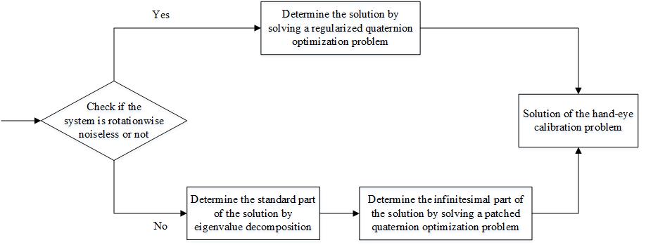
Figure 1: The flow chart of proposed method.

In the next section, we present some preliminary knowledge on dual numbers, quaternions and dual quaternions. Based on dual quaternion optimization, the reformulations and analysis for hand-eye calibration equations $AX=XB$ and $AX=ZB$ are given in Sections 3 and 4, respectively. In Section 5, we present the numerical results to show the efficiency of proposed methods. Some final remarks are made in Section 6.

Throughout the paper, the sets of real numbers, dual numbers, quaternion numbers and dual quaternion numbers are denoted by $\mathbb{R}$, $\mathbb{D}$, $\mathbb{Q}$ and $\mathbb{DQ}$, respectively. The sets of $n$-dimensional real vectors, quaternion vectors and dual quaternion vectors are denoted by ${\mathbb{R}}^{n}$, ${\mathbb{Q}}^{n}$ and ${\mathbb{DQ}}^{n}$, respectively. Scalars, vectors and matrices are denoted by lowercase letters, bold lowercase letters and capital letters, respectively.

2 Preliminaries

2.1 Dual numbers

A dual number $q\in\mathbb{D}$ can be written as $q=q_{st}+q_{\mathcal{I}}\epsilon$, where $q_{st},q_{\mathcal{I}}\in\mathbb{R}$ and $\epsilon$ is the infinitesimal unit satisfying $\epsilon^{2}=0$. We call $q_{st}$ the standard part of $q$, and $q_{\mathcal{I}}$ the infinitesimal part of $q$. Dual numbers can be added component-wise, and multiplied by the formula

$$(p_{st}+p_{\mathcal{I}}\epsilon)(q_{st}+q_{\mathcal{I}}\epsilon)=p_{st}q_{st}+(p_{st}q_{\mathcal{I}}+p_{\mathcal{I}}q_{st})\epsilon.$$

The dual numbers form a commutative algebra of dimension two over the reals. The absolute value of $q=q_{st}+q_{\mathcal{I}}\epsilon\in\mathbb{D}$ is defined as

$$|q|=\left\{\begin{aligned} |q_{st}|+\frac{q_{st}q_{\mathcal{I}}}{|q_{st}|}\epsilon,&\quad{\rm if}\ q_{st}\not=0,\\ |q_{\mathcal{I}}|\epsilon,&\quad{\rm otherwise.}\end{aligned}\right.$$

A total order “$\leq$” for dual numbers was introduced in [24]. Given two dual numbers $p,q\in\mathbb{D}$, $p=p_{st}+p_{\mathcal{I}}\epsilon$, $q=q_{st}+q_{\mathcal{I}}\epsilon$, where $p_{st},p_{\mathcal{I}},q_{st},q_{\mathcal{I}}\in\mathbb{R}$, we say that $p\leq q$, if either $p_{st}<q_{st}$, or $p_{st}=q_{st}$ and $p_{\mathcal{I}}\leq q_{\mathcal{I}}$. In particular, we say that $p$ is positive, nonnegative, nonpositive or negative, if $p>0$, $p\geq 0$, $p\leq 0$ or $p<0$, respectively.

2.2 Quaternion numbers

A quaternion number $q\in\mathbb{Q}$ has the form $q=q_{0}+q_{1}\mathbf{i}+q_{2}\mathbf{j}+q_{3}\mathbf{k},$ where $q_{0},q_{1},q_{2},q_{3}\in\mathbb{R}$ and $\mathbf{i},\mathbf{j},\mathbf{k}$ are three imaginary units of quaternions satisfying

$$\mathbf{i}^{2}=\mathbf{j}^{2}=\mathbf{k}^{2}=\mathbf{i}\mathbf{j}\mathbf{k}=-1,\quad\mathbf{i}\mathbf{j}=-\mathbf{j}\mathbf{i}=\mathbf{k},\quad\mathbf{j}\mathbf{k}=-\mathbf{k}\mathbf{j}=\mathbf{i},\quad\mathbf{k}\mathbf{i}=-\mathbf{i}\mathbf{k}=\mathbf{j}.$$

The conjugate of $q$ is the quaternion $q^{*}=q_{0}-q_{1}\mathbf{i}-q_{2}\mathbf{j}-q_{3}\mathbf{k}$. The scalar part of $q$ is $\text{Sc}(q)=\frac{1}{2}(q+q^{*})=q_{0}$. Clearly, $\text{Sc}(q^{*})=\text{Sc}(q)$ and $(pq)^{*}=q^{*}p^{*}$ for any $p,q\in\mathbb{Q}$. The multiplication of quaternions is associative and distributive over vector addition, but is not commutative. The magnitude of $q$ is

$$|q|=\sqrt{qq^{*}}=\sqrt{q^{*}q}=\sqrt{q_{0}^{2}+q_{1}^{2}+q_{2}^{2}+q_{3}^{2}}.$$

The quaternion $q\in\mathbb{Q}$ is called a unit quaternion if $|q|=1$. It is well-known [33] that the unit quaternion

$$q=\cos\left(\frac{\theta}{2}\right)+\sin\left(\frac{\theta}{2}\right)n_{1}\mathbf{i}+\sin\left(\frac{\theta}{2}\right)n_{2}\mathbf{j}+\sin\left(\frac{\theta}{2}\right)n_{3}\mathbf{k},$$

can be used to described the rotation around a unit axis ${\bf n}=(n_{1},n_{2},n_{3})^{\top}\in\mathbb{R}^{3}$ with an angle of $-\pi\leq\theta\leq\pi$. On the other hand, given a unit quaternion $q=q_{0}+q_{1}\mathbf{i}+q_{2}\mathbf{j}+q_{3}\mathbf{k}\in\mathbb{Q}$, the rotation matrix $R$ can be obtained by

$$R=\left(\begin{array}[]{ccc}q_{0}^{2}+q_{1}^{2}-q_{2}^{2}-q_{3}^{2}&2(q_{1}q_{2}-q_{0}q_{3})&2(q_{1}q_{3}+q_{0}q_{2})\\ 2(q_{1}q_{2}+q_{0}q_{3})&q_{0}^{2}-q_{1}^{2}+q_{2}^{2}-q_{3}^{2}&2(q_{2}q_{3}-q_{0}q_{1})\\ 2(q_{1}q_{3}-q_{0}q_{2})&2(q_{2}q_{3}+q_{0}q_{1})&q_{0}^{2}-q_{1}^{2}-q_{2}^{2}+q_{3}^{2}\end{array}\right).$$ (3)

For any $a=a_{0}+a_{1}\mathbf{i}+a_{2}\mathbf{j}+a_{3}\mathbf{k}\in\mathbb{Q}$, denote $\overrightarrow{a}=(a_{0},a_{1},a_{2},a_{3})^{\top}$ and

$$M(a)=\left(\begin{array}[]{rrrr}a_{0}&-a_{1}&-a_{2}&-a_{3}\\ a_{1}&a_{0}&-a_{3}&a_{2}\\ a_{2}&a_{3}&a_{0}&-a_{1}\\ a_{3}&-a_{2}&a_{1}&a_{0}\end{array}\right),\quad W(a)=\left(\begin{array}[]{rrrr}a_{0}&-a_{1}&-a_{2}&-a_{3}\\ a_{1}&a_{0}&a_{3}&-a_{2}\\ a_{2}&-a_{3}&a_{0}&a_{1}\\ a_{3}&a_{2}&-a_{1}&a_{0}\end{array}\right).$$

Clearly, $|a|=\|\overrightarrow{a}\|_{2}$. By direct calculations, we have the following propositions.

Proposition 2.1.

For any $a=a_{0}+a_{1}\mathbf{i}+a_{2}\mathbf{j}+a_{3}\mathbf{k}\in\mathbb{Q}$ and $b=b_{0}+b_{1}\mathbf{i}+b_{2}\mathbf{j}+b_{3}\mathbf{k}\in\mathbb{Q}$, the following statements hold:

• ${\rm Sc}(r_{1}a+r_{2}b)=r_{1}{\rm Sc}(a)+r_{2}{\rm Sc}(b)$ for any $r_{1},r_{2}\in\mathbb{R}$.

• ${\rm Sc}(a^{*}b)={\rm Sc}(ab^{*})={\rm Sc}(b^{*}a)={\rm Sc}(ba^{*})=\overrightarrow{a}^{\top}\overrightarrow{b}$.

• $M(a^{*})=M(a)^{\top}$, $W(a^{*})=W(a)^{\top}$.

• $\overrightarrow{ab}=M(a)\overrightarrow{b}=W(b)\overrightarrow{a}$.

• $M(a)^{\top}M(a)=W(a)^{\top}W(a)=\|\overrightarrow{a}\|_{2}^{2}I_{4\times 4}$, where $I_{4\times 4}$ is the identity matrix of size $4\times 4$.

Proposition 2.2.

If $a$ and $b$ are two quaternion numbers satisfying $\text{Sc}(a^{*}b)=0$, then for any $q\in\mathbb{Q}$, we have $\text{Sc}(q^{*}a^{*}bq)=\text{Sc}(q^{*}b^{*}aq)=0.$

Proof.

Since $\text{Sc}(a^{*}b)=0$, we have $a^{*}b+b^{*}a=0$. According to Proposition 2.1, one can obtain that $\text{Sc}(q^{*}a^{*}bq)=\text{Sc}(q^{*}b^{*}aq)=\text{Sc}\left(q^{*}(\frac{a^{*}b+b^{*}a}{2})q\right)=0$ for any $q\in\mathbb{Q}.$ ∎

Next we introduce the $2$-norm for quaternion vectors, which can be found in [24]. Denote $\mathbf{x}=(x_{1},x_{2},\cdots,x_{n})^{\top}\in{\mathbb{Q}}^{n}$ for quaternion vectors. The $2$-norm of $\mathbf{x}\in{\mathbb{Q}}^{n}$ is defined as

$$\|\mathbf{x}\|_{2}=\sqrt{\sum_{i=1}^{n}|x_{i}|^{2}}=\sqrt{\sum_{i=1}^{n}\|\overrightarrow{x_{i}}\|_{2}^{2}}.$$

The conjugate transpose of $\mathbf{x}$ is defined as $\mathbf{x}^{*}=(x_{1}^{*},x_{2}^{*},\cdots,x_{n}^{*})$. More details about quaternions and quaternion vectors could be found in [34].

2.3 Dual quaternion numbers

A dual quaternion number $q\in\mathbb{DQ}$ has the form $q=q_{st}+q_{\mathcal{I}}\epsilon$, where $q_{st},q_{\mathcal{I}}\in\mathbb{Q}$. The conjugate of $q=q_{st}+q_{\mathcal{I}}\epsilon$ is $q^{*}=q_{st}^{*}+q_{\mathcal{I}}^{*}\epsilon$. The magnitude of a dual quaternion number $q=q_{st}+q_{\mathcal{I}}\epsilon$ is defined as

$$|q|=\left\{\begin{aligned} |q_{st}|+\frac{{\rm Sc}(q_{st}^{*}q_{\mathcal{I}})}{|q_{st}|}\epsilon,&\quad{\rm if}\ q_{st}\not=0,\\ |q_{\mathcal{I}}|\epsilon,&\quad{\rm otherwise.}\end{aligned}\right.$$

The dual quaternion number $q\in\mathbb{DQ}$ is called a unit dual quaternion if $|q|=1$. Note that $q=q_{st}+q_{\mathcal{I}}\epsilon\in\mathbb{DQ}$ is a unit dual quaternion if and only if $q_{st}^{*}q_{st}=1$ and $q_{st}^{*}q_{\mathcal{I}}+q_{\mathcal{I}}^{*}q_{st}=0$. According to Proposition 2.2, we have the following result.

Corollary 2.3.

If $q=q_{st}+q_{\mathcal{I}}\epsilon\in\mathbb{DQ}$ is a unit dual quaternion, then $\text{Sc}(q_{st}^{*}q_{\mathcal{I}})=\text{Sc}(q_{\mathcal{I}}^{*}q_{st})=0$ and for any $a\in\mathbb{Q}$, we have $\text{Sc}(a^{*}q_{st}^{*}q_{\mathcal{I}}a)=\text{Sc}(a^{*}q_{\mathcal{I}}^{*}q_{st}a)=0.$

It has been shown that the 3D motion of a rigid body can be represented by a unit dual quaternion [7]. Consider a rigid motion in $SE(3)$ represented by a $4\times 4$ homogeneous transformation matrix

$$T=\left(\begin{array}[]{cc}R&{\bf t}\\ {\bf 0}^{\top}&1\end{array}\right),$$ (4)

where $R\in\mathbb{R}^{3\times 3}$ is the rotation matrix about an axis through the origin and ${\bf t}\in\mathbb{R}^{3}$ is the translation vector. Let $q_{st}\in\mathbb{Q}$ be the unit quaternion encoding the rotation matrix $R$ and let $t\in\mathbb{Q}$ be the quaternion satisfying $\overrightarrow{t}=\left(\begin{array}[]{c}0\\ {\bf t}\end{array}\right)$. Then the transformation matrix $T$ is represented by the dual quaternion ${q=q_{st}+q_{\mathcal{I}}\epsilon},$ where $q_{\mathcal{I}}=\frac{1}{2}tq_{st}$. It is not difficult to check that $q\in\mathbb{DQ}$ is a unit dual quaternion since

$${\rm Sc}(q_{st}^{*}q_{\mathcal{I}})=\frac{1}{2}{\rm Sc}(q_{st}^{*}tq_{st})=0.$$

On the other hand, given a unit dual quaternion $q=q_{st}+q_{\mathcal{I}}\epsilon\in\mathbb{DQ}$, the corresponding homogeneous transformation matrix $T$ can be obtained by (4), where the rotation matrix $R\in\mathbb{R}^{3\times 3}$ can be derived from the unit quaternion $q_{st}$ according to (3) and the translation vector ${\bf t}\in\mathbb{R}^{3}$ can be derived from

$$\left(\begin{array}[]{c}0\\ {\bf t}\end{array}\right)=\overrightarrow{2q_{\mathcal{I}}q_{st}^{*}}.$$ (5)

It follows that $\|{\bf t}\|_{2}^{2}=4q_{\mathcal{I}}q_{st}^{*}q_{st}q_{\mathcal{I}}^{*}=4|q_{\mathcal{I}}|^{2}$. In other words, for a unit dual quaternion, the magnitude of its infinitesimal part is half of the length of the corresponding translation vector.

Denote $\mathbf{x}=(x_{1},x_{2},\cdots,x_{n})^{\top}\in{\mathbb{DQ}}^{n}$ for dual quaternion vectors. We may also write

$$\mathbf{x}=\mathbf{x}_{st}+\mathbf{x}_{\mathcal{I}}\epsilon,$$

where $\mathbf{x}_{st},\mathbf{x}_{\mathcal{I}}\in{\mathbb{Q}}^{n}$. The $2$-norm of $\mathbf{x}\in{\mathbb{DQ}}^{n}$ is defined as

$$\|\mathbf{x}\|_{2}=\left\{\begin{aligned} \sqrt{\sum_{i=1}^{n}|x_{i}|^{2}},&\quad{\rm if}\ \mathbf{x}_{st}\not=\mathbf{0},\\ \|\mathbf{x}_{\mathcal{I}}\|_{2}\epsilon,&\quad{\rm otherwise.}\end{aligned}\right.$$ (6)

Denote by $\mathbf{x}^{*}:=(x_{1}^{*},x_{2}^{*},\cdots,x_{n}^{*})$ the conjugate transpose of $\mathbf{x}\in\mathbb{DQ}^{n}$. According to Proposition 6.3 of [24], it holds that

$$\|\mathbf{x}\|_{2}=\|\mathbf{x}_{st}\|_{2}+\frac{\text{Sc}({\mathbf{x}}_{st}^{*}{\mathbf{x}_{\mathcal{I}}})}{\|{\mathbf{x}}_{st}\|_{2}}\epsilon,$$ (7)

for any $\mathbf{x}\in\mathbb{DQ}^{n}$ with $\mathbf{x}_{st}\neq{\bf 0}$.

3 Hand-Eye Calibration Equation $AX=XB$

The hand-eye calibration problem is to find the matrix $X$ such that

$$A^{(i)}X=XB^{(i)},$$ (8)

for $i=1,2,\ldots,n$, where $X$ is transformation matrix from the gripper (hand) to the camera (eye), $A^{(i)}$ is the transformation matrix between the grippers of two different poses and $B^{(i)}$ the transformation matrix between the cameras of two different poses. The transformation matrices $X$, $A^{(i)}$ and $B^{(i)}$ are encoded with the unit dual quaternions

$$x=x_{st}+x_{\mathcal{I}}\epsilon,\quad{a}^{(i)}={a}^{(i)}_{st}+a^{(i)}_{\mathcal{I}}\epsilon,\quad{b}^{(i)}=b^{(i)}_{st}+b^{(i)}_{\mathcal{I}}\epsilon,$$

for $i=1,2,\ldots,n$. Let ${\bf a}=\left(a^{(1)},a^{(2)},\ldots,a^{(n)}\right)^{\top}\in\mathbb{DQ}^{n}$ and ${\bf b}=\left(b^{(1)},b^{(2)},\ldots,b^{(n)}\right)^{\top}\in\mathbb{DQ}^{n}$. The hand-eye calibration problem (8) can be reformulated as the dual quaternion optimization problem

$$\begin{array}[]{cl}\min&\|{\bf a}x-x{\bf b}\|_{2}\\ \text{s.t.}&|x|=1.\end{array}$$ (9)

Denote ${\bf f}(x)={\bf a}x-x{\bf b}\in\mathbb{DQ}^{n}$. According to (6) and (7), we have

$$\|{\bf f}(x)\|_{2}=\left\{\begin{array}[]{ll}\|{\bf f}_{st}(x)\|_{2}+\frac{\text{Sc}\left({\bf f}_{st}^{*}(x){\bf f}_{\mathcal{I}}(x)\right)}{\|{\bf f}_{st}(x)\|_{2}}\epsilon,&\text{if }{\bf f}_{st}(x)\neq{\bf 0},\\ \|{\bf f}_{\mathcal{I}}(x)\|_{2}\epsilon,&\text{otherwise}.\end{array}\right.$$

Problem (9) can be divided to two different cases, which need to be handled very differently. One case is that the standard part of the optimal value of (9) is zero. Another case is that the standard part of the optimal value of (9) is positive. Physically, the standard part of the optimal value of (9) is zero if and only if there exists a “perfect” robot hand motion $x$, which meets all the $n$ testing poses rotationwise exactly. In this case, we say that system is rotationwise noiseless. The following proposition provides a way to check if the system is rotationwise noiseless or not.

Proposition 3.1.

If $\hat{x}$ is an optimal solution of (9), the standard part $\hat{x}_{st}$ is an optimal solution of the quaternion optimization problem

$$\begin{array}[]{cl}\min&\|{\bf a}_{st}x_{st}-x_{st}{\bf b}_{st}\|_{2}^{2}\\ \text{s.t.}&|x_{st}|=1.\end{array}$$ (10)

Hence, the system is rotationwise noiseless if and only if the optimal value of (10) is equal to zero.

Proof.

According to the definition of total order for dual numbers, the result could be easily proved since ${\bf f}_{st}(x)={\bf a}_{st}x_{st}-x_{st}{\bf b}_{st}$ . ∎

Denote the optimal set of (10) by $X_{st}$. If the optimal value of (10) is equal to zero, we consider the regularized quaternion optimization problem

$$\begin{array}[]{cl}\min&\|{\bf f}_{\mathcal{I}}(x)\|_{2}^{2}+\gamma(x_{st}^{*}x_{st}+x_{\mathcal{I}}^{*}x_{\mathcal{I}})\\ \text{s.t.}&x_{st}\in X_{st},\quad x_{st}^{*}x_{\mathcal{I}}+x_{\mathcal{I}}^{*}x_{st}=0.\end{array}$$ (11)

where $\gamma$ is the parameter that balances the loss function and the regularization term. In fact, $x_{st}\in X_{st}$ implies $x_{st}^{*}x_{st}=1$, and $x_{\mathcal{I}}^{*}x_{\mathcal{I}}$ is proportional to the norm square of translation vector. By adding the regularization term, we try to find the best solution with minimal distance of translation. This explains the role of regularization.

If the optimal value of (10) is not equal to zero, we consider the quaternion optimization problem

$$\begin{array}[]{cl}\min&\text{Sc}\left({\bf f}_{st}^{*}(x){\bf f}_{\mathcal{I}}(x)\right)\\ \text{s.t.}&x_{st}\in X_{st},\quad x_{st}^{*}x_{\mathcal{I}}+x_{\mathcal{I}}^{*}x_{st}=0.\end{array}$$ (12)

By using the matrix representation for quaternion numbers, problems (10), (11) and (12) could be solved efficiently. For $i=1,2,\ldots,n$, we have

$$\overrightarrow{a^{(i)}_{st}x_{st}-x_{st}b_{st}^{(i)}}=\left[M\left(a^{(i)}_{st}\right)-W\left(b_{st}^{(i)}\right)\right]\overrightarrow{x_{st}}$$

and

$$\left|a^{(i)}_{st}x_{st}-x_{st}b_{st}^{(i)}\right|^{2}=\overrightarrow{x_{st}}^{\top}\left[M\left(a^{(i)}_{st}\right)-W\left(b_{st}^{(i)}\right)\right]^{\top}\left[M\left(a^{(i)}_{st}\right)-W\left(b_{st}^{(i)}\right)\right]\overrightarrow{x_{st}}.$$

Denote

$$L_{11}=\sum_{i=1}^{n}\left[M\left(a^{(i)}_{st}\right)-W\left(b_{st}^{(i)}\right)\right]^{\top}\left[M\left(a^{(i)}_{st}\right)-W\left(b_{st}^{(i)}\right)\right].$$ (13)

It follows that

$$\|{\bf a}_{st}x_{st}-x_{st}{\bf b}_{st}\|_{2}^{2}=\sum_{i=1}^{n}\left|a^{(i)}_{st}x_{st}-x_{st}b_{st}^{(i)}\right|^{2}=\overrightarrow{x_{st}}^{\top}L_{11}\overrightarrow{x_{st}}.$$

Denote the minimal eigenvalue of matrix $L_{11}$ by $\lambda_{0}$. As a result, problem (10) is equivalent to finding the unit eigenvectors corrresponding to $\lambda_{0}$.

Similarly, for $i=1,2,\ldots,n$, we have

$$\overrightarrow{a_{st}^{(i)}x_{\mathcal{I}}+a_{\mathcal{I}}^{(i)}x_{st}-x_{st}b_{\mathcal{I}}^{(i)}-x_{\mathcal{I}}b_{st}^{(i)}}=\left[M\left(a^{(i)}_{st}\right)-W\left(b_{st}^{(i)}\right)\right]\overrightarrow{x_{\mathcal{I}}}+\left[M\left(a^{(i)}_{\mathcal{I}}\right)-W\left(b_{\mathcal{I}}^{(i)}\right)\right]\overrightarrow{x_{st}}.$$

Denote

$$L_{22}=\sum_{i=1}^{n}\left[M\left(a^{(i)}_{\mathcal{I}}\right)-W\left(b_{\mathcal{I}}^{(i)}\right)\right]^{\top}\left[M\left(a^{(i)}_{\mathcal{I}}\right)-W\left(b_{\mathcal{I}}^{(i)}\right)\right]$$ (14)

and

$$L_{12}=\sum_{i=1}^{n}\left[M\left(a^{(i)}_{st}\right)-W\left(b_{st}^{(i)}\right)\right]^{\top}\left[M\left(a^{(i)}_{\mathcal{I}}\right)-W\left(b_{\mathcal{I}}^{(i)}\right)\right].$$ (15)

It follows that

$$\|{\bf f}_{\mathcal{I}}(x)\|_{2}^{2}=\sum_{i=1}^{n}\left|a_{st}^{(i)}x_{\mathcal{I}}+a_{\mathcal{I}}^{(i)}x_{st}-x_{st}b_{\mathcal{I}}^{(i)}-x_{\mathcal{I}}b_{st}^{(i)}\right|^{2}=\overrightarrow{x_{\mathcal{I}}}^{\top}L_{11}\overrightarrow{x_{\mathcal{I}}}+2\overrightarrow{x_{\mathcal{I}}}^{\top}L_{12}\overrightarrow{x_{st}}+\overrightarrow{x_{st}}^{\top}L_{22}\overrightarrow{x_{st}}.$$

As a result, problem (11) is equivalent to the optimization problem

$$\begin{array}[]{cl}\min&\overrightarrow{x_{\mathcal{I}}}^{\top}(L_{11}+\gamma I)\overrightarrow{x_{\mathcal{I}}}+2\overrightarrow{x_{\mathcal{I}}}^{\top}L_{12}\overrightarrow{x_{st}}+\overrightarrow{x_{st}}^{\top}(L_{22}+\gamma I)\overrightarrow{x_{st}}\\ \text{s.t.}&\overrightarrow{x_{st}}\in\overrightarrow{X_{st}},\quad\overrightarrow{x_{st}}^{\top}\overrightarrow{x_{\mathcal{I}}}=0,\end{array}$$ (16)

where $\overrightarrow{X_{st}}$ is the set of all the unit eigenvectors corrresponding to the minimal eigenvalue of matrix $L_{11}$. Once the set $\overrightarrow{X_{st}}$ is determinated, problem (16) turns out to be a quadratically constrained quadratic program (QCQP).

To be specific, suppose that the dimension of the eigenspace of the minimal eigenvalue of $L_{11}$ is $k$. Let $Q\in\mathbb{R}^{4\times k}$ be the matrix whose columns form an orthonormal basis of the eigenspace, i.e., $Q^{\top}Q=I_{k\times k}$. It is not difficult to see that $\overrightarrow{X_{st}}=\{Q\mathbf{y}:\mathbf{y}^{\top}\mathbf{y}=1,\mathbf{y}\in\mathbb{R}^{k}\}$. Problem (16) can be rewritten as

$$\begin{array}[]{cl}\min&\overrightarrow{x_{\mathcal{I}}}^{\top}(L_{11}+\gamma I)\overrightarrow{x_{\mathcal{I}}}+2\overrightarrow{x_{\mathcal{I}}}^{\top}L_{12}Q\mathbf{y}+\mathbf{y}^{\top}Q^{\top}(L_{22}+\gamma I)Q\mathbf{y}\\ \text{s.t.}&{\mathbf{y}}^{\top}\mathbf{y}=1,\quad\mathbf{y}^{\top}Q^{\top}\overrightarrow{x_{\mathcal{I}}}=0.\end{array}$$ (17)

In particular, if the dimension of the eigenspace is one, i.e., $k=1$, the solution set $\overrightarrow{X_{st}}=\{{\bf q},-{\bf q}\}$, where $\bf q\in\mathbb{R}^{4}$ is the normalized basis of the eigenspace. In this case, problem (17) could be solved efficiently by representing $\overrightarrow{x_{\mathcal{I}}}$ in the orthogonal complement space of $\bf q$.

In the following, we reformulate problem (12) as an optimization problem by using the matrix representation for quaternion numbers. According to Proposition 2.1, we have

$$\text{Sc}\left(\left(a^{(i)}_{st}x_{st}-x_{st}b_{st}^{(i)}\right)^{*}\left(a_{st}^{(i)}x_{\mathcal{I}}+a_{\mathcal{I}}^{(i)}x_{st}-x_{st}b_{\mathcal{I}}^{(i)}-x_{\mathcal{I}}b_{st}^{(i)}\right)\right)$$

$$=\overrightarrow{x_{st}}^{\top}\left[M\left(a^{(i)}_{st}\right)-W\left(b_{st}^{(i)}\right)\right]^{\top}\left[M\left(a^{(i)}_{st}\right)-W\left(b_{st}^{(i)}\right)\right]\overrightarrow{x_{\mathcal{I}}}$$

$$\hskip 113.81102pt+\overrightarrow{x_{st}}^{\top}\left[M\left(a^{(i)}_{st}\right)-W\left(b_{st}^{(i)}\right)\right]^{\top}\left[M\left(a^{(i)}_{\mathcal{I}}\right)-W\left(b_{\mathcal{I}}^{(i)}\right)\right]\overrightarrow{x_{st}}$$

for $i=1,2,\ldots,n$. It follows that

$$\text{Sc}\left({\bf f}_{st}^{*}(x){\bf f}_{\mathcal{I}}(x)\right) =\sum_{i=1}^{n}\text{Sc}\left(\left(a^{(i)}_{st}x_{st}-x_{st}b_{st}^{(i)}\right)^{*}\left(a_{st}^{(i)}x_{\mathcal{I}}+a_{\mathcal{I}}^{(i)}x_{st}-x_{st}b_{\mathcal{I}}^{(i)}-x_{\mathcal{I}}b_{st}^{(i)}\right)\right)$$

$$=\overrightarrow{x_{st}}^{\top}L_{11}\overrightarrow{x_{\mathcal{I}}}+\overrightarrow{x_{st}}^{\top}L_{12}\overrightarrow{x_{st}},$$

where $L_{11}$ and $L_{12}$ are given by (13) and (15) respectively. Note that $\overrightarrow{X_{st}}$ is the set of all unit eigenvectors corresponding to the minimal eigenvalue $\lambda_{0}$ of $L_{11}$. Under the constraints of (12), one can obtain that

$$\overrightarrow{x_{st}}^{\top}L_{11}\overrightarrow{x_{\mathcal{I}}}=\lambda_{0}\overrightarrow{x_{st}}^{\top}\overrightarrow{x_{\mathcal{I}}}=0,$$

since $L_{11}$ is symmetric. It turns out that problem (12) is equivalent to the optimization problem

$$\begin{array}[]{cl}\min&\overrightarrow{x_{st}}^{\top}L_{12}\overrightarrow{x_{st}}\\ \text{s.t.}&\overrightarrow{x_{st}}\in\overrightarrow{X_{st}},\quad\overrightarrow{x_{st}}^{\top}\overrightarrow{x_{\mathcal{I}}}=0.\end{array}$$ (18)

Similarly, if $Q$ is the matrix whose columns form an orthonormal basis of the eigenspace of $\lambda_{0}$, the optimal $\overrightarrow{x_{st}}$ can be derived by computing the unit eigenvectors corresponding to the minimal eigenvalue of $\text{Sym}\left(Q^{\top}L_{12}Q\right)=\left(Q^{\top}L_{12}Q+Q^{\top}L_{12}^{\top}Q\right)/2$. Since the objective function in (18) does not contain $\overrightarrow{x_{\mathcal{I}}}$ , the optimal $\overrightarrow{x_{\mathcal{I}}}$ can be any vector which is orthogonal to the optimal $\overrightarrow{x_{st}}$. We may need to find a proper one via sewing a patch on the optimal set of $\overrightarrow{x_{\mathcal{I}}}$, while ensuring that $\|{\bf f}_{st}(x)\|_{2}$ is minimized. Considering the continuity of the norm, it is naturally necessary to further search for $x_{\mathcal{I}}$ under the constrains of $\overrightarrow{x_{st}}^{\top}\overrightarrow{x_{\mathcal{I}}}=0$, such that $\|{\bf f}_{\mathcal{I}}(x)\|_{2}$ is reduced as much as possible, i.e.,

$$\begin{array}[]{cl}\min_{\overrightarrow{x_{\mathcal{I}}}}&\overrightarrow{x_{\mathcal{I}}}^{\top}L_{11}\overrightarrow{x_{\mathcal{I}}}+2\overrightarrow{x_{\mathcal{I}}}^{\top}L_{12}\overrightarrow{x_{st}}+\overrightarrow{x_{st}}^{\top}L_{22}\overrightarrow{x_{st}}\\ \text{s.t.}&\overrightarrow{x_{st}}^{\top}\overrightarrow{x_{\mathcal{I}}}=0.\end{array}$$ (19)

This explains the role of the patching.

Note that in this way, we give a complete description for the solution set of the hand-eye calibration problem. This is new in the hand-eye calibration literature and should be useful in applications.

To conclude, the solution method for hand-eye calibration equation $AX=XB$ is summarized in Algorithm 1.

0:  Motions $\left(A^{(i)},B^{(i)}\right)_{i=1}^{n}$, regularization parameter $\gamma$.

0:  The hand-eye transformation matrix $X$.

1:  Construct the matrix $L_{11},L_{22}$ and $L_{12}$ according to (13), (14) and (15), respectively.

2:  Compute the minimal eigenvalue $\lambda_{0}$ of $L_{11}$, and deduce the orthonormal basis $Q$ for the eigenspace of $\lambda_{0}$.

3:  if  $\lambda_{0}=0$  then

4:     Compute $x_{st}$ and $x_{\mathcal{I}}$ by solving QCQP (17).

5:  else

6:     Compute $x_{st}$ by finding the unit eigenvector corresponding to the minimal eigenvalue of $\text{Sym}\left(Q^{\top}L_{12}Q\right)$.

7:     Compute $x_{\mathcal{I}}$ by solving (19) with the optimal $x_{st}$.

8:  end if

9:  Compute $X=\left(\begin{array}[]{cc}R&{\bf t}\\ {\bf 0}^{\top}&1\end{array}\right)$, where $R$ is computed from $x_{st}$ by (3) and $\bf t$ is computed from $x_{st}$ and $x_{\mathcal{I}}$ by using (5).

Algorithm 1 Dual quaternion optimization for $AX=XB$

4 Hand-Eye Calibration Equation $AX=ZB$

In 1994, Zhuang, Roth and Sudhaker [38] generalized (1) to $AX=ZB$, where $X$ is transformation matrix from the gripper to the camera, $Z$ is the transformation matrix from the robot base to the world coordinate system, $A$ is the transformation matrix from the robot base to the gripper and $B$ is the transformation matrix from the world base to the camera. Given $n$ measurements $\left(A^{(i)},B^{(i)}\right)_{i=1}^{n}$, the problem is to find the best solution $X$ and $Z$ such that

$$A^{(i)}X=ZB^{(i)},$$ (20)

for $i=1,2,\ldots,n$. The transformation matrices $X$, $Z$, $A^{(i)}$ and $B^{(i)}$ are encoded with the unit dual quaternions

$$x=x_{st}+x_{\mathcal{I}}\epsilon,\quad z=z_{st}+z_{\mathcal{I}}\epsilon,\quad{a}^{(i)}={a}^{(i)}_{st}+a^{(i)}_{\mathcal{I}}\epsilon,\quad{b}^{(i)}=b^{(i)}_{st}+b^{(i)}_{\mathcal{I}}\epsilon,$$

for $i=1,2,\ldots,n$. Let ${\bf a}=\left(a^{(1)},a^{(2)},\ldots,a^{(n)}\right)^{\top}\in\mathbb{DQ}^{n}$ and ${\bf b}=\left(b^{(1)},b^{(2)},\ldots,b^{(n)}\right)^{\top}\in\mathbb{DQ}^{n}$. The hand-eye calibration problem (20) can be reformulated as the dual quaternion optimization problem

$$\begin{array}[]{cl}\min&\|{\bf a}x-z{\bf b}\|_{2}\\ \text{s.t.}&|x|=|z|=1.\end{array}$$ (21)

Similarly, we say that the system is rotationwise noiseless if and only if the standard part of the optimal value of (21) is zero.

Denote ${\bf g}(x,z)={\bf a}x-z{\bf b}\in\mathbb{DQ}^{n}$. To solve problem (21), according to the definition of 2-norm for dual quaternion vectors, we first consider the quaternion optimization problem

$$\begin{array}[]{cl}\min&\|{\bf g}_{st}(x,z)\|_{2}^{2}=\|{\bf a}_{st}x_{st}-z_{st}{\bf b}_{st}\|_{2}^{2}\\ \text{s.t.}&|x_{st}|=|z_{st}|=1.\end{array}$$ (22)

Note that $a=a_{st}+a_{\mathcal{I}}\epsilon\in\mathbb{DQ}$ is a unit dual quaternion if and only if $a_{st}^{*}a_{st}=1$ and $\text{Sc}\left(a_{st}^{*}a_{\mathcal{I}}\right)=a_{st}^{*}a_{\mathcal{I}}+a_{\mathcal{I}}^{*}a_{st}=0$. For $i=1,2,\ldots,n$, we have

$$\left|a^{(i)}_{st}x_{st}-z_{st}b_{st}^{(i)}\right|^{2} =\left(a^{(i)}_{st}x_{st}-z_{st}b_{st}^{(i)}\right)^{*}\left(a^{(i)}_{st}x_{st}-z_{st}b_{st}^{(i)}\right)$$

$$=2-2\text{Sc}\left(x_{st}^{*}\left(a_{st}^{(i)}\right)^{*}z_{st}b_{st}^{(i)}\right)$$

$$=2-2\overrightarrow{x_{st}}^{\top}M\left(a_{st}^{(i)}\right)^{\top}W\left(b_{st}^{(i)}\right)\overrightarrow{z_{st}}$$

since $x$, $z$, $a^{(i)}$ and $b^{(i)}$ are unit dual quaternions. Denote

$$K_{11}=\sum_{i=1}^{n}M\left(a_{st}^{(i)}\right)^{\top}W\left(b_{st}^{(i)}\right).$$ (23)

It follows that

$$\|{\bf a}_{st}x_{st}-z_{st}{\bf b}_{st}\|_{2}^{2}=\sum_{i=1}^{n}\left|a^{(i)}_{st}x_{st}-z_{st}b_{st}^{(i)}\right|^{2}=2n-2\overrightarrow{x_{st}}^{\top}K_{11}\overrightarrow{z_{st}}.$$

Then problem (22) is equivalent to the optimization problem

$$\begin{array}[]{cl}\max&\overrightarrow{x_{st}}^{\top}K_{11}\overrightarrow{z_{st}}\\ \text{s.t.}&\overrightarrow{x_{st}}^{\top}\overrightarrow{x_{st}}=\overrightarrow{z_{st}}^{\top}\overrightarrow{z_{st}}=1.\end{array}$$ (24)

Denote the maximal singular value of $K_{11}$ by $\sigma_{1}$, the set of optimal vector pairs of (24) by $\overrightarrow{\Omega_{st}}$. As a result, problem (22) is to find the unit singular vector pairs for $\sigma_{1}$, which can be solved efficiently by the singular value decomposition (SVD).

If the optimal value of (22) is equal to zero, i.e., $\sigma_{1}=n$, consider the regularized optimization problem

$$\begin{array}[]{cl}\min&\|{\bf g}_{\mathcal{I}}(x,z)\|_{2}^{2}+\gamma\left(x_{st}^{*}x_{st}+x_{\mathcal{I}}^{*}x_{\mathcal{I}}+z_{st}^{*}z_{st}+z_{\mathcal{I}}^{*}z_{\mathcal{I}}\right)\\ \text{s.t.}&\left(\overrightarrow{x_{st}},\overrightarrow{z_{st}}\right)\in\overrightarrow{\Omega_{st}},\quad\overrightarrow{x_{st}}^{\top}\overrightarrow{x_{\mathcal{I}}}=0,\quad\overrightarrow{z_{st}}^{\top}\overrightarrow{z_{\mathcal{I}}}=0,\end{array}$$ (25)

where $\gamma$ is the regularization parameter and

$$\|{\bf g}_{\mathcal{I}}(x,z)\|_{2}^{2}=\sum_{i=1}^{n}\left\|M\left(a_{st}^{(i)}\right)\overrightarrow{x_{\mathcal{I}}}+M\left(a_{\mathcal{I}}^{(i)}\right)\overrightarrow{x_{st}}-W\left(b_{\mathcal{I}}^{(i)}\right)\overrightarrow{z_{st}}-W\left(b_{st}^{(i)}\right)\overrightarrow{z_{\mathcal{I}}}\right\|_{2}^{2}.$$

Once the set $\overrightarrow{\Omega_{st}}$ is determined, problem (25) could be also written as an QCQP. To be specific, suppose the singular value decomposition of matrix $K_{11}$ is $K_{11}=U\Sigma V^{\top}$, where $U,V\in\mathbb{R}^{4\times 4}$ are orthogonal and $\Sigma\in\mathbb{R}^{4\times 4}$ is diagonal. Let $Q_{1}\in\mathbb{R}^{4\times k}$ be the matrix whose columns are the columns of $U$ corresponding to $\sigma_{1}$, and let $Q_{2}\in\mathbb{R}^{4\times k}$ be the matrix whose columns are the columns of $V$ corresponding to $\sigma_{1}$. It is not difficult to see that $\overrightarrow{\Omega_{st}}=\left\{\left(Q_{1}\mathbf{y},Q_{2}\mathbf{y}\right):\mathbf{y}^{\top}\mathbf{y}=1,\mathbf{y}\in\mathbb{R}^{k}\right\}$. In fact, for any unit vectors $\mathbf{y}_{1}$ and $\mathbf{y}_{2}$, the value of objective function of (24) at the point $\left(\overrightarrow{x_{st}},\overrightarrow{z_{st}}\right)=\left(Q_{1}\mathbf{y}_{1},Q_{2}\mathbf{y}_{2}\right)$ is

$$\overrightarrow{x_{st}}^{\top}K_{11}\overrightarrow{z_{st}}=\mathbf{y}_{1}^{\top}Q_{1}^{\top}K_{11}Q_{2}\mathbf{y}_{2}=\sigma_{1}\mathbf{y}_{1}^{\top}\mathbf{y}_{2}\leq\sigma_{1},$$

according to the Cauchy-Schwarz inequality. Without loss of generality, we assume $\sigma_{1}>0$. Then the equality holds if and only if $\mathbf{y}_{1}=\mathbf{y}_{2}$. As a result, problem (25) can be rewritten as an QCQP:

$$\begin{array}[]{cl}\min&\displaystyle\sum_{i=1}^{n}\left\|M\left(a_{st}^{(i)}\right)\overrightarrow{x_{\mathcal{I}}}+M\left(a_{\mathcal{I}}^{(i)}\right)Q_{1}\mathbf{y}-W\left(b_{\mathcal{I}}^{(i)}\right)Q_{2}\mathbf{y}-W\left(b_{st}^{(i)}\right)\overrightarrow{z_{\mathcal{I}}}\right\|_{2}^{2}+\gamma\left(\overrightarrow{x_{\mathcal{I}}}^{\top}\overrightarrow{x_{\mathcal{I}}}+\overrightarrow{z_{\mathcal{I}}}^{\top}\overrightarrow{z_{\mathcal{I}}}+2\mathbf{y}^{\top}\mathbf{y}\right)\\ \text{s.t.}&\mathbf{y}^{\top}\mathbf{y}=1,\quad\mathbf{y}^{\top}Q_{1}^{\top}\overrightarrow{x_{\mathcal{I}}}=0,\quad\mathbf{y}^{\top}Q_{2}^{\top}\overrightarrow{z_{\mathcal{I}}}=0.\end{array}$$ (26)

In particular, when $k=1$, problem (26) could be solved efficiently by representing $\overrightarrow{x_{\mathcal{I}}}$ and $\overrightarrow{z_{\mathcal{I}}}$ in the corresponding orthogonal complement space of $Q_{1}$ and $Q_{2}$, respectively.

On the other hand, if the optimal value of (22) is not equal to zero, consider the optimization problem

$$\begin{array}[]{cl}\min&\text{Sc}\left({\bf g}_{st}^{*}(x,z){\bf g}_{\mathcal{I}}(x,z)\right)\\ \text{s.t.}&\left(\overrightarrow{x_{st}},\overrightarrow{z_{st}}\right)\in\overrightarrow{\Omega_{st}},\quad\overrightarrow{x_{st}}^{\top}\overrightarrow{x_{\mathcal{I}}}=0,\quad\overrightarrow{z_{st}}^{\top}\overrightarrow{z_{\mathcal{I}}}=0.\end{array}$$ (27)

According to Corollary 2.3, we have

$$\text{Sc}\left(\left(a^{(i)}_{st}x_{st}\right)^{*}a_{st}^{(i)}x_{\mathcal{I}}\right)=\text{Sc}\left(\left(a^{(i)}_{st}x_{st}\right)^{*}a_{\mathcal{I}}^{(i)}x_{st}\right)=\text{Sc}\left(\left(z_{st}b_{st}^{(i)}\right)^{*}z_{st}b_{\mathcal{I}}^{(i)}\right)=\text{Sc}\left(\left(z_{st}b_{st}^{(i)}\right)^{*}z_{\mathcal{I}}b_{st}^{(i)}\right)=0$$

since $x$, $z$, $a^{(i)}$ and $b^{(i)}$ are unit quaternions for $i=1,2,\ldots,n$. It follows that

$$\text{Sc}\left(\left(a^{(i)}_{st}x_{st}-z_{st}b_{st}^{(i)}\right)^{*}\left(a_{st}^{(i)}x_{\mathcal{I}}+a_{\mathcal{I}}^{(i)}x_{st}-z_{st}b_{\mathcal{I}}^{(i)}-z_{\mathcal{I}}b_{st}^{(i)}\right)\right)$$

$$=-\text{Sc}\left(\left(a^{(i)}_{st}x_{st}\right)^{*}z_{st}b_{\mathcal{I}}^{(i)}+\left(a^{(i)}_{st}x_{st}\right)^{*}z_{\mathcal{I}}b_{st}^{(i)}+\left(z_{st}b_{st}^{(i)}\right)^{*}a_{st}^{(i)}x_{\mathcal{I}}+\left(z_{st}b_{st}^{(i)}\right)^{*}a_{\mathcal{I}}^{(i)}x_{st}\right)$$

$$=-\overrightarrow{x_{st}}^{\top}\left[M\left(a_{st}^{(i)}\right)^{\top}W\left(b_{\mathcal{I}}^{(i)}\right)+M\left(a_{\mathcal{I}}^{(i)}\right)^{\top}W\left(b_{st}^{(i)}\right)\right]\overrightarrow{z_{st}}$$

$$\hskip 113.81102pt-\overrightarrow{x_{st}}^{\top}M\left(a_{st}^{(i)}\right)^{\top}W\left(b_{st}^{(i)}\right)\overrightarrow{z_{\mathcal{I}}}-\overrightarrow{x_{\mathcal{I}}}^{\top}M\left(a_{st}^{(i)}\right)^{\top}W\left(b_{st}^{(i)}\right)\overrightarrow{z_{st}}.$$

Denote

$$K_{12}=\sum_{i=1}^{n}M\left(a_{st}^{(i)}\right)^{\top}W\left(b_{\mathcal{I}}^{(i)}\right)$$ (28)

and

$$K_{21}=\sum_{i=1}^{n}M\left(a_{\mathcal{I}}^{(i)}\right)^{\top}W\left(b_{st}^{(i)}\right).$$ (29)

By simple computation, one can obtain that

$$\text{Sc}\left({\bf g}_{st}^{*}(x,z){\bf g}_{\mathcal{I}}(x,z)\right) =\sum_{i=1}^{n}\text{Sc}\left(\left(a^{(i)}_{st}x_{st}-z_{st}b_{st}^{(i)}\right)^{*}\left(a_{st}^{(i)}x_{\mathcal{I}}+a_{\mathcal{I}}^{(i)}x_{st}-z_{st}b_{\mathcal{I}}^{(i)}-z_{\mathcal{I}}b_{st}^{(i)}\right)\right)$$

$$=-\left[\overrightarrow{x_{st}}^{\top}(K_{12}+K_{21})\overrightarrow{z_{st}}+\overrightarrow{x_{st}}^{\top}K_{11}\overrightarrow{z_{\mathcal{I}}}+\overrightarrow{x_{\mathcal{I}}}^{\top}K_{11}\overrightarrow{z_{st}}\right],$$

where $K_{11}$, $K_{12}$ and $K_{21}$ are given by (23), (28) and (29), respectively. Under the constraints of problem (27), $\overrightarrow{x_{st}}$ and $\overrightarrow{z_{st}}$ are left-singular and right-singular vectors corresponding to the maximal singular value $\sigma_{1}$ for $K_{11}$, which means

$$K_{11}\overrightarrow{z_{st}}=\sigma_{1}\overrightarrow{x_{st}}\quad\text{and}\quad K_{11}^{\top}\overrightarrow{x_{st}}=\sigma_{1}\overrightarrow{z_{st}}.$$

Then we have $\overrightarrow{x_{st}}^{\top}K_{11}\overrightarrow{z_{\mathcal{I}}}=\sigma_{1}\overrightarrow{z_{st}}^{\top}\overrightarrow{z_{\mathcal{I}}}=0$ and $\overrightarrow{x_{\mathcal{I}}}^{\top}K_{11}\overrightarrow{z_{st}}=\sigma_{1}\overrightarrow{x_{\mathcal{I}}}^{\top}\overrightarrow{x_{st}}=0$ under the constraints of problem (27). As a result, problem (27) is equivalent to the optimization

$$\begin{array}[]{cl}\max&\overrightarrow{x_{st}}^{\top}(K_{12}+K_{21})\overrightarrow{z_{st}}\\ \text{s.t.}&\left(\overrightarrow{x_{st}},\overrightarrow{z_{st}}\right)\in\overrightarrow{\Omega_{st}},\quad\overrightarrow{x_{st}}^{\top}\overrightarrow{x_{\mathcal{I}}}=0,\quad\overrightarrow{z_{st}}^{\top}\overrightarrow{z_{\mathcal{I}}}=0.\end{array}$$ (30)

Similarly, given the singular value decomposition $K_{11}=U\Sigma V^{\top}$, let $Q_{1}$ be the matrix whose columns are the columns of $U$ corresponding to $\sigma_{1}$, and let $Q_{2}$ be the matrix whose columns are the columns of $V$ corresponding to $\sigma_{1}$. The optimal $\overrightarrow{x_{st}}$ and $\overrightarrow{z_{st}}$ can be derived by computing the unit eigenvectors corresponding to the maximal eigenvalue of $\text{Sym}\left(Q_{1}^{\top}(K_{12}+K_{21})Q_{2}\right)$. Since the objective funcion in (30) does not contain $\overrightarrow{x_{\mathcal{I}}}$ and $\overrightarrow{z_{\mathcal{I}}}$, the optimal $\overrightarrow{x_{\mathcal{I}}}$ can be any vector which is orthogonal to the optimal $\overrightarrow{x_{st}}$, and the optimal $\overrightarrow{z_{\mathcal{I}}}$ can be any vector which is orthogonal to the optimal $\overrightarrow{z_{st}}$. Considering the continuity of the norm, once the optimal $\overrightarrow{x_{st}}$ and $\overrightarrow{z_{st}}$ are determined, we try to find the best one in the optimal set of $\overrightarrow{x_{\mathcal{I}}}$ and $\overrightarrow{z_{\mathcal{I}}}$ such that the patching function $\|{\bf g}_{\mathcal{I}}(x,z)\|_{2}^{2}$ is minimized, i.e.,

$$\begin{array}[]{cl}\max_{\overrightarrow{x_{\mathcal{I}}},\overrightarrow{z_{\mathcal{I}}}}&\displaystyle\sum_{i=1}^{n}\left\|M\left(a_{st}^{(i)}\right)\overrightarrow{x_{\mathcal{I}}}+M\left(a_{\mathcal{I}}^{(i)}\right)\overrightarrow{x_{st}}-W\left(b_{\mathcal{I}}^{(i)}\right)\overrightarrow{z_{st}}-W\left(b_{st}^{(i)}\right)\overrightarrow{z_{\mathcal{I}}}\right\|_{2}^{2}\\ \text{s.t.}&\overrightarrow{x_{st}}^{\top}\overrightarrow{x_{\mathcal{I}}}=0,\quad\overrightarrow{z_{st}}^{\top}\overrightarrow{z_{\mathcal{I}}}=0.\end{array}$$ (31)

To conclude, the solution method for hand-eye calibration equation $AX=ZB$ is summarized in Algorithm 2.

0:  Measurements $\left(A^{(i)},B^{(i)}\right)_{i=1}^{n}$, regularization parameter $\gamma$.

0:  The hand-eye transformation matrix $X$ and robort-word transformation matrix $Z$.

1:  Construct the matrix $K_{11},K_{12}$ and $K_{21}$ according to (23), (28) and (29), respectively.

2:  Compute SVD for $K_{11}$, and deduce the maximal singular value $\sigma_{1}$ with corresponding column-orthogonal matrices $Q_{1}$ and $Q_{2}$.

3:  if  $\sigma_{1}=n$  then

4:     Compute $x_{st},z_{st},x_{\mathcal{I}}$ and $z_{\mathcal{I}}$ by solving QCQP (26).

5:  else

6:     Compute $x_{st}$ and $z_{st}$ by finding the unit eigenvector corresponding to the maximal eigenvalue of $\text{Sym}\left(Q_{1}^{\top}(K_{12}+K_{21})Q_{2}\right)$.

7:     Compute $x_{\mathcal{I}}$ and $z_{\mathcal{I}}$ by solving (31) with the optimal $x_{st}$ and $z_{st}$.

8:  end if

9:  Compute $X$ and $Z$ from the dual quaternions $x=x_{st}+x_{\mathcal{I}}\epsilon$ and $z=z_{st}+z_{\mathcal{I}}\epsilon$ respectively.

Algorithm 2 Dual quaternion optimization for $AX=ZB$

5 Numerical Experiments

In this section, we report a set of synthetic experiments to show the efficiency of proposed methods for hand-eye calibration problem. All the codes are written in Matlab R2017a. The numerical experiments were done on a desktop with an Intel Core i5-2430M CPU dual-core processor running at 2.4GHz and 6GB of RAM.

In the implementation of our proposed methods, we use GloptiPoly [13] to construct SDP relaxations of QCQPs, and use MOSEK [21] as SDP solver. Further, GloptiPoly can also recover the solution to the original problem and certify its optimality. We set the regularization parameter $\gamma=2\times 10^{-6}$. For hand-eye calibration model $AX=XB$, we compare our method with the direct estimation proposed by Tsai et al. [30] (denoted by “Tsai89”), the Kronecker method proposed by Andreff et al. [1] (denoted by “Andreff99”), the classic dual quaternion method proposed by Daniilidis [7] (denoted by “Daniilidis99”), the improved dual quaternion method proposed by Malti et al. [20] (denoted by “Malti10”), and the dual quaternion method using polynomial optimization proposed by Heller et al. [12] (denoted by “Heller14”).

For hand-eye calibration model $AX=ZB$, we compare our method with the quaternion method proposed by Zhuang et al. [38] (denoted by “Zhuang94”), the quaternion method proposed by Dornaika et al. [9] (denoted by “Dornaika98”), the classic dual quaternion method proposed by Li et al. [16] (denoted by “Li10”), the dual quaternion method using polynomial optimization proposed by Heller et al. [12] (denoted by “Heller14”), and the dual quaternion method proposed by Li et al. [17] (denoted by “Li18”).

Numerical experiments are carried out as follows. First, the original homogeneous transformation matrices $\hat{X}$ and $\hat{Z}$ in (2) are given by

$$\hat{X}=\left(\begin{array}[]{rrrr}0.9995&-0.0100&0.0297&9.190\\ 0.0116&0.9986&-0.0523&5.397\\ -0.0291&0.0526&0.9982&0\\ 0&0&0&1.0000\\ \end{array}\right),$$ (32)

and

$$\hat{Z}=\left(\begin{array}[]{rrrr}0.2790&-0.0981&-0.9553&164.226\\ -0.5439&0.8037&-0.2414&301.638\\ 0.7914&0.5869&0.1709&0\\ 0&0&0&1.0000\end{array}\right).$$ (33)

Second, we generate $n$ transformation matrices $A^{(i)}$, $i=1,2,\ldots,n$. Then the transformation matrix $B^{(i)}$ is computed by $B^{(i)}=\hat{Z}^{-1}A^{(i)}\hat{X}$ for $i=1,2,\ldots,n$. We use different methods to solve the hand-eye calibration equation $AX=ZB$ with the given matrices $\left(A^{(i)},B^{(i)}\right)_{i=1}^{n}$. For hand-eye calibration equation $AX=XB$, we construct $\frac{n(n-1)}{2}$ pairs of matrices $\left(\left(A^{(i)}\right)^{-1}A^{(j)},\left(B^{(i)}\right)^{-1}B^{(j)}\right)_{i<j}$, denoted by $\left(\tilde{A}^{(s)},\tilde{B}^{(s)}\right)_{s=1}^{n(n-1)/2}$. Then different methods are used to solve the hand-eye calibration equation $AX=XB$ with the given matrices $\left(\tilde{A}^{(s)},\tilde{B}^{(s)}\right)_{s=1}^{n(n-1)/2}$. The estimation errors are computed by

$$e_{X}=\|X-\hat{X}\|_{2},\quad e_{Z}=\|Z-\hat{Z}\|_{2}.$$

5.1 Measurements with non-parallel rotation axis

Four measurements of $A$ with non-parallel rotation axis are given by

$$A^{(1)}=\left(\begin{array}[]{rrrr}0.1752&-0.6574&0.7329&-10.5536\\ 0.6325&-0.4954&-0.5954&-30.5304\\ 0.7545&0.5679&0.3290&50.4851\\ 0&0&0&1.0000\end{array}\right),$$

$$A^{(2)}=\left(\begin{array}[]{rrrr}-0.0745&0.9661&0.2471&-20.4123\\ 0.8573&-0.0645&0.5108&-50.8904\\ 0.5094&0.2499&-0.8234&80.8685\\ 0&0&0&1.0000\end{array}\right),$$

$$A^{(3)}=\left(\begin{array}[]{rrrr}-0.1456&-0.6867&0.7122&-20.5519\\ 0.8252&-0.4814&-0.2955&-30.6491\\ 0.5458&0.5447&0.6367&60.4312\\ 0&0&0&1.0000\end{array}\right),$$

$$A^{(4)}=\left(\begin{array}[]{rrrr}-0.1434&-0.5250&0.8389&-10.5892\\ 0.8158&-0.5427&-0.2001&-50.6730\\ 0.5603&0.6557&0.5061&80.4641\\ 0&0&0&1.0000\end{array}\right).$$

As described above, we have four measurements $\left(A^{(i)},B^{(i)}\right)$ for equation $AX=ZB$, and six motions $\left(\tilde{A}^{(s)},\tilde{B}^{(s)}\right)$ for equation $AX=XB$. The numerical results for $AX=XB$ and $AX=ZB$ with non-parallel rotation axis are reported in Tables 1 and 2, respectively. The proposed Algorithms 1 and 2 show the best behavior in terms of estimation error. Note that the first three methods in Table 1 and the first three methods in Table 2 get the solution via solving linear equations, while the other methods need to call SDP solvers to get the solution. That explains why Algorithm 1 may need more computation time to get the solution when compared with the first three methods in Table 1, and Algorithm 2 may need more computation time to get the solution when compared with the first three methods in Table 2.

Table 1: Numerical results for $AX=XB$ with non-parallel rotation axis

	Tsai89	Andreff99	Daniilidis99	Malti10	Heller14	Alg. 1
$e_{X}$	0.0030	0.0027	0.0014	0.0019	0.0014	0.0003
Time(s)	0.0419	0.0188	0.0747	3.8888	1.4171	1.1649

Table 2: Numerical results for $AX=ZB$ with non-parallel rotation axis

	Zhuang94	Dornaika98	Li10	Heller14	Li18	Alg. 2
$e_{X}$	0.0010	0.0362	0.0005	0.0012	0.0029	0.0004
$e_{Z}$	0.0135	0.0712	0.0155	0.0138	0.0142	0.0132
Time(s)	0.0200	0.0190	0.0761	40.3641	1.9992	1.0494

5.2 Measurements with parallel rotation axis

In this subsection, we test our algorithms for the case that all the axes of measurements are parallel, which is often the situation for the han-eye calibration of SCARA robots [31]. In this case, it has been shown that the problem is not well-defined and there exists a 1D manifold of equivalent solutions with identical algebraic error [2, 35]. To evaluate the quality of solutions, we try to find the solution such that the third component of its translation vector is equal to zero, and then compare it with the real solution $\hat{X}$ and $\hat{Z}$ given by (32) and (33), respectively.

Four measurements of $A$ are generated with the same rotation axis, but with different angles. Without loss of generality, the normalized rotation axis is ${\bf n}=(0,0,1)^{\top}$. For $A^{(1)},A^{(2)},A^{(3)},A^{(4)}$, the rotation angles are $\theta_{1}=\frac{\pi}{6}$, $\theta_{2}=\frac{\pi}{3}$, $\theta_{3}=-\frac{\pi}{6}$ and $\theta_{4}-\frac{\pi}{3}$, while their translation vectors are randomly generated given by

$${\bf t}_{1}=(-10.9865,12.3788,-27.2571)^{\top},\quad{\bf t}_{2}=(38.8986,84.6736,-93.8814)^{\top},$$

$${\bf t}_{3}=(-75.7189,-53.6187,28.5794)^{\top},\quad{\bf t}_{4}=(-52.8133,93.3732,-70.1666)^{\top},$$

respectively. The numerical results for $AX=XB$ and $AX=ZB$ with parallel rotation axis are reported in Tables 3 and 4, respectively.

Table 3: Numerical results for $AX=XB$ with parallel rotation axis

	Tsai89	Andreff99	Daniilidis99	Malti10	Heller14	Alg. 1
$e_{X}$	11.8042	57.2739	0.0042	44.1233	0.0042	0.0040
Time(s)	0.0566	0.0212	0.2014	3.8501	1.3656	1.1441

Table 4: Numerical results for $AX=ZB$ with parallel rotation axis

	Zhuang94	Dornaika98	Li10	Heller14	Li18	Alg. 2
$e_{X}$	45.3702	112.3677	0.0064	0.0068	21.8262	0.0023
$e_{Z}$	259.5928	642.9365	0.0125	0.0382	124.8814	0.0128
Time(s)	0.0191	0.0179	0.0839	39.2364	2.2217	1.5278

5.3 Measurement estimation with noise

In practice, the measurement of $B$ is typically estimated using visual processing. Since visual estimation is noisy, this set of experiment aims comparing the robustness of the different methods to disturbances in the measurement of $B$.

The four measurements $\left(A^{(i)},B^{(i)}\right)_{i=1}^{4}$ are the same with that in Subsection 5.1. The rotation and translation of $B^{(i)}$ are disturbed by adding zero mean Gaussian noise with increasing standard deviation. Note that the motions $\tilde{B}^{(s)}$ are also disturbed when adding noise to the measurements $B^{(i)}$. The standard deviation of the additive noise increases from 0 to 0.02 in steps of 0.002. For each standard deviation, the average errors of $e_{X}$ and $e_{Z}$ are recorded after 10 runs of each method. The robustness testing for $AX=XB$ and $AX=ZB$ with noisy measurements of $B$ are plotted in Figures 2 and 3, respectively.

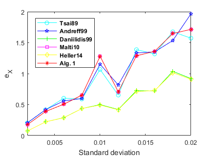
Figure 2: Robustness testing for $AX=XB$.

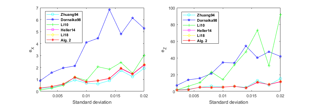
Figure 3: Robustness testing for $AX=ZB$.

6 Final Remarks

In this paper, we establish a new dual quaternion optimization method for the hand-eye calibration problem based on the 2-norm of dual quaternion vectors. A two-stage method is also proposed by using the techniques of regularization and patching. However, there are still some problems that need further study. We have the following final remarks.

1. Can we use some other norms for dual quaternion vectors, e.g. 1-norm, $\infty$-norm, instead of 2-norm in this method?

2. We may also consider some other hand-eye calibration models, such as multi-camera hand-eye calibration.

3. How can we choose the regularization parameter $\gamma$ to improve the efficiency of the method?

4. Can we extend this method to the simultaneous localization and mapping problem?

Acknowledgment. We are very thankful to Wei Li for helpful discussion and providing the data and Matlab code for the methods in [17].

References

• [1] Andreff N, Horaud R and Espiau B, “Robot hand-eye calibration using structure-from-motion”, The International Journal of Robotics Research 21 (2001) 228-248.
• [2] Chen H H, “A screw motion approach to uniqueness analysis of head-eye geometry”, 1991 IEEE Computer Society Conference on Computer Vision and Pattern Recognition (1991) 145-151.
• [3] Chou J C K and Kamel M, “Quaternions approach to solve the kinematic equation of rotation, $A_{a}A_{x}=A_{x}A_{b}$, of a sensor-mounted robotic manipulator”, 1988 IEEE International Conference on Robotics and Automation (1988) 656-662.
• [4] Chou J C K and Kamel M, “Finding the position and orientation of a sensor on a robot manipulator using quaternions”, The International Journal of Robotics Research 10(3) (1991) 240-254.
• [5] Condurache D and Burlacu A, “Orthogonal dual tensor method for solving the $AX=XB$ sensor calibration problem”, Mechanism and Machine Theory 104 (2016) 382-404.
• [6] Condurache D and Ciureanu I A, “A novel solution for $AX=YB$ sensor calibration problem using dual Lie algebra”, 2019 6th International Conference on Control, Decision and Information Technologies (CoDIT) (2019) 302-307.
• [7] Daniilidis K, “Hand-eye calibration using dual quaternions”, The International Journal of Robotics Research 18(3) (1999) 286-298.
• [8] Daniilidis K and Bayro-Corrochano E, “The dual quaternion approach to hand-eye calibration”, 13th International Conference on Pattern Recognition 1 (1996) 318-322.
• [9] Dornaika F and Horaud R, “Simultaneous robot-world and hand-eye calibration”, IEEE transactions on Robotics and Automation 14(4) (1998) 617-622.
• [10] Enebuse I, Foo M, Ibrahim B K S M K, et al., “A comparative review of hand-eye calibration techniques for vision guided robots”, IEEE Access 9 (2021) 113143-113155.
• [11] Gwak S, Kim J and Park F C, “Numerical optimization on the Euclidean group with applications to camera calibration”, IEEE Transactions on Robotics and Automation 19(1) (2003) 65-74.
• [12] Heller J, Henrion D and Pajdla T, “Hand-eye and robot-world calibration by global polynomial optimization”, 2014 IEEE International Conference on Robotics and Automation (ICRA) (2014) 3157-3164.
• [13] Henrion D, Lasserre J B and Löfberg J, “GloptiPoly 3: moments, optimization and semidefinite programming”, Optimization Methods & Software 24(4-5) (2009) 761-779.
• [14] Horaud R and Dornaika F, “Hand-eye calibration”, The International Journal of Robotics Research 14(3) (1995) 195-210.
• [15] Jiang J, Luo X, Luo Q, et al., “An overview of hand-eye calibration”, The International Journal of Advanced Manufacturing Technology (2021) 1-21.
• [16] Li A, Wang L and Wu D, “Simultaneous robot-world and hand-eye calibration using dual-quaternions and Kronecker product”, International Journal of Physical Sciences 5(10) (2010) 1530-1536.
• [17] Li W, Lv N, Dong M and Lou X, “Simultaneous robot-world/hand-eye calibration using dual quaternion”, Robot (in Chinese) 40(3) (2018) 301-308.
• [18] Liang R and Mao J, “Hand-eye calibration with a new linear decomposition algorithm”, Journal of Zhejiang University-SCIENCE A 9(10) (2008) 1363-1368.
• [19] Lu Y C and Chou J C K, “Eight-space quaternion approach for robotic hand-eye calibration”, 1995 IEEE International Conference on Systems, Man and Cybernetics. Intelligent Systems for the 21st Century 4 (1995) 3316-3321.
• [20] Malti A and Barreto J P, “Robust hand-eye calibration for computer aided medical endoscopy”, 2010 IEEE International Conference on Robotics and Automation (2010) 5543-5549.
• [21] MOSEK Aps, The MOSEK optimization toolbox for MATLAB (Version 9.3). www.mosek.com.
• [22] Park F C and Martin B J, “Robot sensor calibration: solving $AX=XB$ on the Euclidean group”, IEEE Transactions on Robotics and Automation 10(5) (1994) 717-721.
• [23] Qi L, “Standard dual quaternion optimization and its applications in hand-eye calibration and SLAM”, Communications on Applied Mathematics and Computaion DOI: 10.1007/s42967-022-00213-1.
• [24] Qi L, Ling C, Yan H. “Dual quaternions and dual quaternion vectors”, Communications on Applied Mathematics and Computation 4 (2022) 1494-1508.
• [25] Remy S, Dhome M, Lavest J M and Daucher N, “Hand-eye calibration”, 1997 IEEE/RSJ International Conference on Intelligent Robot and Systems, Innovative Robotics for Real-World Applications, IROS’97 2 (1997) 1057-1065.
• [26] Schmidt J, Vogt F and Niemann H, “Robust hand–eye calibration of an endoscopic surgery robot using dual quaternions”, Joint Pattern Recognition Symposium (2003) 548-556.
• [27] Shah M, Eastman R D and Hong T, “An overview of robot-sensor calibration methods for evaluation of perception systems”, Proceedings of the Workshop on Performance Metrics for Intelligent Systems (2012) 15-20.
• [28] Shah M, “Solving the robot-world/hand-eye calibration problem using the Kronecker product”, Journal of Mechanisms and Robotics 5(3) (2013) 031007.
• [29] Shiu Y C and Ahmad S, “Calibration of wrist-mounted robotic sensors by solving homogeneous transform equations of the form $AX=XB$”, IEEE Transactions on Robotics and Automation 5(1) (1989) 16-29.
• [30] Tsai R Y and Lenz R K, “A new technique for fully autonomous and efficient 3d robotics hand/eye calibration”, IEEE Transactions on Robotics and Automation 5(3) (1989) 345-358.
• [31] Ulrich M and Steger C, “Hand-eye calibration of SCARA robots using dual quaternions”, Pattern Recognition and Image Analysis 26(1) (2016) 231-239.
• [32] Wang C C, “Extrinsic calibration of a vision sensor mounted on a robot”, IEEE Transactions on Robotics and Automation 8(2) (1992) 161-175.
• [33] Wang X and Zhu H, “On the comparisons of unit dual quaternion and homogeneous transformation matrix”, Advances in Applied Clifford Algebras 24(1) (2014) 213-229.
• [34] Wei M, Li Y, Zhang F and Zhao J, “Quaternion Matrix Computations”, Nova Science Publishers, New York, 2018.
• [35] Zhang H, “Hand/eye calibration for electronic assembly robots”, IEEE Transactions on Robotics and Automation 14(4) (1998) 612-616.
• [36] Zhang Z, Zhang L and Yang G Z, “A computationally efficient method for hand–eye calibration”, International Journal of Computer Assisted Radiology and Surgery 12(10) (2017) 1775-1787.
• [37] Zhao Z, “Simultaneous robot-world and hand-eye calibration by the alternative linear programming”, Pattern Recognition Letters 127 (2019) 174-180.
• [38] Zhuang H, Roth Z and Sudhakar R, “Simultaneous robot-world and tool/flange calibration by solving homogeneous transformation of the form $AX=YB$”, IEEE Transactions on Robotics and Automation 10(4) (1994) 549-554.
• [39] Zhuang H and Shiu Y C, “A noise-tolerant algorithm for robotic hand-eye calibration with or without sensor orientation measurement”, IEEE Transactions on Systems, Man, and Cybernetics 23(4) (1993) 1168-1175.