On Stochastic Orders and Total Positivity

Abstract

The usual stochastic order and the likelihood ratio order between probability distributions on the real line are reviewed in full generality. In addition, for the distribution of a random pair $(X,Y)$, it is shown that the conditional distributions of $Y$, given $X=x$, are increasing in $x$ with respect to the likelihood ratio order if and only if the joint distribution of $(X,Y)$ is totally positive of order two (TP2) in a certain sense. It is also shown that these three types of constraints are stable under weak convergence, and that weak convergence of TP2 distributions implies convergence of the conditional distributions just mentioned.

Keywords:

Conditional distribution, likelihood ratio order, order constraint, weak convergence.

AMS 2000 subject classifications:

60E15, 62E10, 62H05.

1 Introduction

In nonparametric statistics, shape-constraints on distributions offer an interesting alternative to more traditional smoothness constraints. Specifically, consider a univariate regression setting with a generic observation $(X,Y)\in\mathbb{R}\times\mathbb{R}$. In many applications it is a natural constraint that the conditional distribution $Q(\cdot\,|\,x):=\mathcal{L}(Y\,|\,X=x)$ is increasing in $x\in\mathbb{R}$ with respect to some order on the set of probability distributions on the real line. Mösching and Dümbgen (2020) analyze estimators of $Q(\cdot\,|\,x)$ under the sole assumption that it is increasing in $x$ with respect to the usual stochastic order, and Mösching and Dümbgen (2022) investigate the same estimation problem under the stronger constraint that $Q(\cdot\,|\,x)$ is increasing in $x$ with respect to the likelihood ratio order.

The likelihood ratio order has also received attention in nonparametric methods for two- or $k$-sample problems, for instance, Dardanoni and Forcina (1998), Westling et al. (2022) and Hu et al. (2022).

One goal of this paper is to review stochastic order, likelihood ratio order and their properties and relations in full generality, extending previous results presented by Shaked and Shanthikumar (2007). Here are precise definitions of these orders, where $Q_{1},Q_{2}$ denote arbitrary probability distributions on the real line:

Stochastic order:

$Q_{1}\leq_{\rm st}Q_{2}$ if $Q_{1}((y,\infty))\leq Q_{2}((y,\infty))$ for all $y\in\mathbb{R}$.

Likelihood ratio order:

$Q_{1}\leq_{\rm lr}Q_{2}$ if $Q_{1},Q_{2}$ admit densities $g_{1},g_{2}$ with respect to some dominating measure such that $g_{2}/g_{1}$ is increasing on $\{g_{1}+g_{2}>0\}$.

It is known and will be explained later that $Q_{1}\leq_{\rm lr}Q_{2}$ implies that $Q_{1}\leq_{\rm st}Q_{2}$. Note that likelihood ratio ordering is familiar from discriminant analysis and mathematical statistics, see Karlin and Rubin (1956) and Lehmann and Romano (2005). Suppose that $Q_{1}\leq_{\rm lr}Q_{2}$. If we observe $(Y,C)\in\mathbb{R}\times\{1,2\}$, where $\mathcal{L}(Y\,|\,C=c)=Q_{c}$, then the posterior probability $\operatorname{\mathbb{P}}(C=2\,|\,Y)$ is isotonic in $Y$. If we observe $Y\sim Q_{\theta}$ with an unknown parameter $\theta\in\{1,2\}$, then an optimal test of the null hypothesis that $\theta=1$ versus the alternative hypothesis that $\theta=2$ rejects the former for large values of $Y$. Furthermore, likelihood ratio ordering is a frequent assumption or implication of models in mathematical finance, see Beare and Moon (2015) and Jewitt (1991).

The notion of likelihood ratio order and its relation to stochastic order is reviewed thoroughly in Section 2, showing that it defines a partial order on the set of all probability measures on the real line which is preserved under weak convergence. No restrictions on the distributions are needed. It is also explained that two distributions are likelihood ratio ordered if and only if the corresponding receiving operator characteristic (ROC) is a concave curve, and this is related to convexity of their ordinal dominance curve. The latter results generalize previous work, e.g. by Westling et al. (2022).

Another goal of this paper is to fully understand the relationship between the distribution of a random pair $(X,Y)$ and order constraints on the conditional distributions $Q(\cdot\,|\,x)$, $x\in\mathbb{R}$. In Section 3 it is shown how to characterize $\mathcal{L}(X,Y)$ such that $Q(\cdot\,|\,x)$ is increasing in $x$ with respect to stochastic order or likelihood ratio order. In particular, we explain the connection between likelihood ratio ordering and total positivity of order two (TP2) of bivariate distributions. Finally, it is shown that these properties of bivariate distributions are preserved under weak convergence, and that this implies convergence of the conditional distributions. To the best of our knowledge, most of the material in Section 3 is completely new.

All proofs are deferred to Section 4.

2 Likelihood ratio order

Let $Q_{1}$ and $Q_{2}$ be probability measures on $\mathbb{R}$, equipped with its Borel $\sigma$-field $\mathcal{B}$. Our first result provides various equivalent conditions for $Q_{1}\leq_{\rm lr}Q_{2}$, the first of which is the definition given in the introduction.

Theorem 1.

The following four conditions on $Q_{1}$ and $Q_{2}$ are equivalent:
(i) There exist a $\sigma$-finite measure $\mu$ and densities $g_{j}=\mathrm{d}Q_{j}/\mathrm{d}\mu$ ($j=1,2$) such that

$$g_{2}/g_{1}\ \ \text{is isotonic on}\ \ \{g_{1}+g_{2}>0\}.$$

(ii) There exist a $\sigma$-finite measure $\mu$ and densities $g_{j}=\mathrm{d}Q_{j}/\mathrm{d}\mu$ ($j=1,2$) such that

$$g_{1}(y)g_{2}(x)\ \leq\ g_{1}(x)g_{2}(y)\quad\text{whenever}\ x<y.$$

(iii) For arbitrary sets $A,B\in\mathcal{B}$ such that $A<B$ (element-wise),

$$Q_{1}(B)Q_{2}(A)\ \leq\ Q_{1}(A)Q_{2}(B).$$

(iv) There exists a dense subset $D$ of $\mathbb{R}$ such that for all intervals $A=(x,y]$ and $B=(y,z]$ with endpoints $x<y<z$ in $D$,

$$Q_{1}(B)Q_{2}(A)\ \leq\ Q_{1}(A)Q_{2}(B).$$

Remark 2.

Shaked and Shanthikumar (2007) restrict their attention to probability measures which are either discrete or dominated by Lebesgue measure. Their definition of likelihood ratio order corresponds to properties (i–ii) with $\mu$ being counting measure or Lebesgue measure on the real line.

Remark 3 (Weak convergence).

An important aspect of Theorem 1 is that conditions (iii-iv) do not involve an explicit dominating measure or explicit densities of $Q_{1}$ and $Q_{2}$. In particular, if $(Q_{n1})_{n}$ and $(Q_{n2})_{n}$ are sequences of distributions on $\mathbb{R}$ converging weakly to $Q_{1}$ and $Q_{2}$, respectively, and if $Q_{n1}\leq_{\rm lr}Q_{n2}$ for all $n$, then $Q_{1}\leq_{\rm lr}Q_{2}$ as well. This follows from (iv) with $D$ being the set of all $x\in\mathbb{R}$ such that $Q_{1}(\{x\})=0=Q_{2}(\{x\})$.

Remark 4 (Stochastic order).

The likelihood ratio order is stronger than the stochastic order in the sense that $Q_{1}\leq_{\rm st}Q_{2}$ if $Q_{1}\leq_{\rm lr}Q_{2}$. This follows immediately from condition (iii) applied to $A:=(-\infty,y]$ and $B:=(y,\infty)$ for arbitrary $y\in\mathbb{R}$, because $Q_{1}(B)Q_{2}(A)=Q_{1}(B)-Q_{1}(B)Q_{2}(B)$ and $Q_{1}(A)Q_{2}(B)=Q_{2}(B)-Q_{1}(B)Q_{2}(B)$.

The reverse statement is false in general, but the likelihood ratio order of two distributions is tightly connected to stochastic order of domain-conditional distributions.

Lemma 5.

The following four properties of $Q_{1}$ and $Q_{2}$ are equivalent:
(i)  $Q_{1}\leq_{\rm lr}Q_{2}$.
(ii)  $Q_{1}(\cdot\,|\,C)\leq_{\rm lr}Q_{2}(\cdot\,|\,C)$ for all sets $C\in\mathcal{B}$ such that $Q_{1}(C),Q_{2}(C)>0$.
(iii)  $Q_{1}(\cdot\,|\,C)\leq_{\rm st}Q_{2}(\cdot\,|\,C)$ for all sets $C\in\mathcal{B}$ such that $Q_{1}(C),Q_{2}(C)>0$.
(iv)  There exists a dense subset $D$ of $\mathbb{R}$ such that $Q_{1}(\cdot\,|\,(x,y])\leq_{\rm st}Q_{2}(\cdot\,|\,(x,y])$ for arbitrary points $x<y$ in $D$ such that $Q_{1}((x,y]),Q_{2}((x,y])>0$.

The next result shows that the relation $\leq_{\rm lr}$ defines indeed a partial order on the space of arbitrary probability measures on the real line.

Lemma 6.

For arbitrary probability measures $Q_{1},Q_{2},Q_{3}$ on $\mathbb{R}$,

$$Q_{1}\leq_{\rm lr}Q_{1} \text{(reflexivity)};$$

$$Q_{1}\leq_{\rm lr}Q_{2}\ \ \text{and}\ \ Q_{2}\leq_{\rm lr}Q_{1}\ \ \text{implies that}\ \ Q_{1}=Q_{2} \text{(antisymmetry)};$$

$$Q_{1}\leq_{\rm lr}Q_{2}\ \ \text{and}\ \ Q_{2}\leq_{\rm lr}Q_{3}\ \ \text{implies that}\ \ Q_{1}\leq_{\rm lr}Q_{3} \text{(transitivity)}.$$

Another interesting aspect of the likelihood ratio order is its connection with the receiver operating characteristic (ROC) of a pair $(Q_{1},Q_{2})$, that means, the set

$$\mathrm{ROC}(Q_{1},Q_{2})\ :=\ \bigl{\{}\bigl{(}Q_{1}(H),Q_{2}(H)\bigr{)}:H\in\mathcal{H}\bigr{\}}$$

with $\mathcal{H}$ denoting the set of left-bounded half-lines, augmented by $\emptyset$ and $\mathbb{R}$,

$$\mathcal{H}\ :=\ \bigl{\{}(y,\infty):y\in\mathbb{R}\bigr{\}}\cup\bigl{\{}[y,\infty):y\in\mathbb{R}\bigr{\}}\cup\{\emptyset,\mathbb{R}\}.$$

Note that the family $\mathcal{H}$ is totally ordered by inclusion. With the distribution function $G_{j}$ of $Q_{j}$ ($j=1,2$) one may also write

$$\mathrm{ROC}(Q_{1},Q_{2})$$

$$\ =\ \bigl{\{}\bigl{(}1-G_{1}(y),1-G_{2}(y)\bigr{)}:y\in\bar{\mathbb{R}}\bigr{\}}\cup\bigl{\{}\bigl{(}1-G_{1}(y\,-),1-G_{2}(y\,-)\bigr{)}:y\in\mathbb{R}\bigr{\}},$$

where $\bar{\mathbb{R}}:=[-\infty,\infty]$ and $G_{j}(-\infty):=0$, $G_{j}(\infty):=1$. Thus we take the freedom to refer to $\mathrm{ROC}(Q_{1},Q_{2})$ as the ROC curve of $Q_{1}$ and $Q_{2}$, imagining a (possibly non-continuous) curve within the unit square $[0,1]\times[0,1]$, connecting the points $(1,1)$ and $(0,0)$.

Obviously, the ROC curve is isotonic in the sense that if $(a_{1},a_{2}),(b_{1},b_{2})\in\mathrm{ROC}(Q_{1},Q_{2})$, then $(a_{1},a_{2})\leq(b_{1},b_{2})$ or $(a_{1},a_{2})\geq(b_{1},b_{2})$ component-wise. By means of Theorem 1, one can easily show that likelihood ratio order is equivalent to a concavity property of the ROC curve.

Corollary 7.

Two distributions $Q_{1},Q_{2}$ satisfy $Q_{1}\leq_{\rm lr}Q_{2}$ if and only if $\mathrm{ROC}(Q_{1},Q_{2})$ is concave in the following sense: If $(a_{1},a_{2})$, $(b_{1},b_{2})$ and $(c_{1},c_{2})$ are three different points in $\mathrm{ROC}(Q_{1},Q_{2})$ with $a_{1}\leq b_{1}\leq c_{1}$ and $a_{2}\leq b_{2}\leq c_{2}$, then

$$\frac{b_{2}-a_{2}}{b_{1}-a_{1}}\ \geq\ \frac{c_{2}-b_{2}}{c_{1}-b_{1}}.$$

An object related to the ROC curve of $Q_{1},Q_{2}$ is the ordinal dominance curve $H_{G_{1},G_{2}}:[0,1]\to[0,1]$,

$$H_{G_{1},G_{2}}(\alpha)\ :=\ G_{2}\bigl{(}G_{1}^{-1}(\alpha)\bigr{)},$$

where $G_{j}^{-1}(\alpha):=\min\{y\in\bar{\mathbb{R}}:G_{j}(y)\geq\alpha\}$. The next result has been shown by Lehmann and Rojo (1992) in the special case of $Q_{2}\ll Q_{1}$ and $G_{1},G_{2}$ being continuous and strictly increasing, where $Q_{2}\ll Q_{1}$ means that $Q_{2}$ admits a density with respect to $Q_{1}$. Westling et al. (2022) proved the same result under the assumption that $Q_{2}\ll Q_{1}$ with a density $\mathrm{d}Q_{2}/\mathrm{d}Q_{1}$ which is continuous on the support of $Q_{1}$.

Corollary 8.

Suppose that $Q_{2}\ll Q_{1}$. Then $Q_{1}\leq_{\rm lr}Q_{2}$ if and only if the ordinal dominance curve $H_{G_{1},G_{2}}$ is convex on the image of $G_{1}$, i.e. the set $G_{1}(\bar{\mathbb{R}})=\{G_{1}(y):y\in\bar{\mathbb{R}}\}$.

Remark 9.

The assumption that $Q_{2}\ll Q_{1}$ is essential in Corollary 8. For instance, if $Q_{1}=(\delta_{0}+\delta_{1})/2$ with $\delta_{y}$ denoting Dirac measure at $y$ and $Q_{2}=\mathrm{Unif}(0,1)$, then $H_{G_{1},G_{2}}(0)=H_{G_{1},G_{2}}(1/2)=0$ and $H_{G_{1},G_{2}}(1)=1$. In consequence, the ordinal dominance curve restricted to $G_{1}(\bar{\mathbb{R}})=\{0,1/2,1\}$ is convex, but $Q_{1}$ is not smaller than $Q_{2}$ with respect to likelihood ratio order since $\mathrm{ROC}(Q_{1},Q_{2})=\{(0,0),(1,1)\}\cup\{(1/2,u):0\leq u\leq 1\}$ is not concave.

Example 10.

Let $Q_{1}=\mathcal{N}(1,1)$ and $Q_{2}=\mathcal{N}(3,6)$. Here $\log dQ_{2}/dQ_{1}(y)$ is strictly convex in $y\in\mathbb{R}$ with limit $\infty$ as $|y|\to\infty$, whence neither $Q_{1}\leq_{\rm lr}Q_{2}$ nor $Q_{2}\leq_{\rm lr}Q_{1}$. The left panel of Figure 1 shows the corresponding ROC curve $\mathrm{ROC}(Q_{1},Q_{2})$ which is obviously not concave. Now let us replace these Gaussian distributions with gamma distributions, $Q_{1}=\mathrm{Gamma}(\alpha_{1},\beta_{1})$ and $Q_{2}=\mathrm{Gamma}(\alpha_{2},\beta_{2})$, where $\mathrm{Gamma}(\alpha,\beta)$ denotes the gamma distribution with shape parameter $\alpha>0$ and scale parameter $\beta>0$. One can easily show that $\log dQ_{2}/dQ_{1}(y)$ is strictly increasing in $y>0$ if $\alpha_{1}\leq\alpha_{2}$, $\beta_{1}\leq\beta_{2}$ and $(\alpha_{1},\beta_{1})\neq(\alpha_{2},\beta_{2})$. The right panel of Figure 1 shows the concave ROC curve for $(\alpha_{1},\beta_{1})=(1,1)$ and $(\alpha_{2},\beta_{2})=(1.5,2)$, i.e. the first and second moments of $Q_{1}$ and $Q_{2}$ coincide with those of the Gaussian distributions considered before.

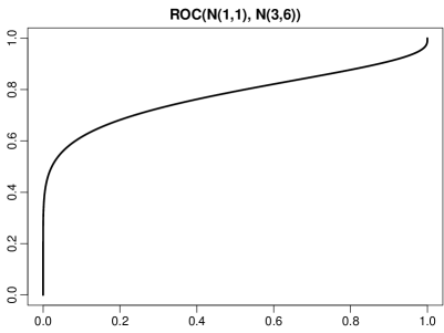
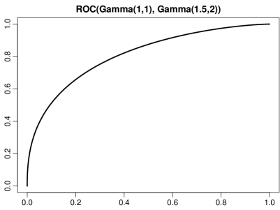
Figure 1: ROC curves for two pairs $(Q_{1},Q_{2})$.

3 Bivariate distributions

Throughout this section we consider a pair $(X,Y)$ of real-valued random variables with distribution $R=\mathcal{L}(X,Y)$ and marginal distributions $P=\mathcal{L}(X)$ and $Q=\mathcal{L}(Y)$. We investigate order constraints on the conditional distributions of $Y$, given that $X$ lies in certain regions. The range of the random variable $X$ is defined as the set

$$\mathcal{X}\ :=\ \bigl{\{}x\in\mathbb{R}:\operatorname{\mathbb{P}}(X\leq x),\operatorname{\mathbb{P}}(X\geq x)>0\bigr{\}}.$$

One can easily verify that $\mathcal{X}$ is the smallest real interval such that $P(\mathcal{X})=\operatorname{\mathbb{P}}(X\in\mathcal{X})=1$.

3.1 Conditional distributions and order constraints

It is well-known from measure theory that the conditional distribution of $Y$, given $X$, may be described by a stochastic kernel $K:\mathbb{R}\times\mathcal{B}\to[0,1]$. That is,

• for any fixed $x\in\mathbb{R}$, $K(x,\cdot)$ is a probability measure on $\mathcal{B}$;

• for any fixed $B\in\mathcal{B}$, $K(\cdot,B)$ is measurable on $\mathbb{R}$;

• for arbitrary $A,B\in\mathcal{B}$,

  $$R(A\times B)\ =\ \int_{A}K(x,B)\,P(\mathrm{d}x).$$

The following two theorems clarify under which conditions on the distribution $R$ of $(X,Y)$, the conditional distribution $K(x,\cdot)$ is isotonic in $x\in\mathcal{X}$ with respect to stochastic order or likelihood ratio order. Interestingly, the proof is constructive, showing that

$$K(x,(y,\infty))\ =\ \sup_{a<x\colon P((a,x])>0}\operatorname{\mathbb{P}}(Y>y\,|\,a<X\leq x)$$

for $x\in\mathcal{X}$ and $y\in\mathbb{R}$.

Theorem 11 (Stochastic order).

The following three conditions are equivalent:

(i)

For arbitrary sets $A_{1},A_{2}\in\mathcal{B}$ with $A_{1}<A_{2}$ and real numbers $y$,

(1) $$R(A_{1}\times(y,\infty))P(A_{2})\ \leq\ P(A_{1})R(A_{2}\times(y,\infty)).$$

(ii)

There exists a dense subset $D$ of $\mathbb{R}$ such that for arbitrary numbers $x_{0}<x_{1}<x_{2}$ and $y$ in $D$, (1) holds true with $A_{1}=(x_{0},x_{1}]$ and $A_{2}=(x_{1},x_{2}]$.

(iii)

The stochastic kernel $K$ may be constructed such that for arbitrary $x_{1},x_{2}\in\mathcal{X}$ with $x_{1}<x_{2}$,

$$K(x_{1},\cdot)\ \leq_{\rm st}\ K(x_{2},\cdot).$$

Remark 12.

Note that $P(A_{j})=R(A_{j}\times(-\infty,y])+R(A_{j}\times(y,\infty))$, so inequality (1) is equivalent to

(2) $$R(A_{1}\times(y,\infty))R(A_{2}\times(-\infty,y])\ \leq\ R(A_{1}\times(-\infty,y])R(A_{2}\times(y,\infty)).$$

This underlines the connection to the next theorem about likelihood ratio order.

Theorem 13 (Likelihood ratio order).

The following three conditions are equivalent:

(i)

For arbitrary Borel sets $A_{1},A_{2},B_{1},B_{2}$ with $A_{1}<A_{2}$ and $B_{1}<B_{2}$,

(3) $$R(A_{1}\times B_{2})R(A_{2}\times B_{1})\ \leq\ R(A_{1}\times B_{1})R(A_{2}\times B_{2}).$$

(ii)

There exists a dense subset $D$ of $\mathbb{R}$ such that for arbitrary numbers $x_{0}<x_{1}<x_{2}$ and $y_{0}<y_{1}<y_{2}$ in $D$, (3) holds true with $A_{1}=(x_{0},x_{1}]$, $A_{2}=(x_{1},x_{2}]$ and $B_{1}=(y_{0},y_{1}]$, $B_{2}=(y_{1},y_{2}]$.

(iii)

The stochastic kernel $K$ may be constructed such that for arbitrary $x_{1},x_{2}\in\mathcal{X}$ with $x_{1}<x_{2}$,

$$K(x_{1},\cdot)\ \leq_{\rm lr}\ K(x_{2},\cdot).$$

Remark 14.

Condition (i) in Theorems 11 and 13 is equivalent to the following statement about conditional distributions: Let $A_{1},A_{2}$ be arbitrary Borel sets such that $A_{1}<A_{2}$ and $P(A_{1})$, $P(A_{2})$ are strictly positive. Then,

$$\mathcal{L}(Y\,|\,X\in A_{1})\ \leq_{\rm st}\ \mathcal{L}(Y\,|\,X\in A_{2})\quad\text{(Theorem~{}\ref{Thm:Kernel.st})},$$

$$\mathcal{L}(Y\,|\,X\in A_{1})\ \leq_{\rm lr}\ \mathcal{L}(Y\,|\,X\in A_{2})\quad\text{(Theorem~{}\ref{Thm:Kernel.lr})}.$$

Condition (ii) in Theorems 11 and 13 may be re-interpreted analogously.

3.2 Total positivity of order two

Theorem 13 hints at a connection between likelihood ratio ordering and total positivity. A good starting point for the latter concept is the monograph of Karlin (1968). Recall that a function $h:\mathbb{R}\times\mathbb{R}\to\mathbb{R}$ is called totally positive of order two (TP2) if for arbitrary real numbers $x_{1}<x_{2}$ and $y_{1}<y_{2}$,

(4) $$h(x_{2},y_{1})h(x_{1},y_{2})\ \leq\ h(x_{1},y_{1})h(x_{2},y_{2}).$$

Thus, conditions (i) and (ii) of Theorem 13 may be interpreted as a distributional notion of total positivity of order two.

Definition 15 (Total positivity of order two of bivariate distributions).

A probability distribution $R$ on $\mathbb{R}\times\mathbb{R}$ is called totally positive of order two (TP2) if for arbitrary Borel sets $A_{1}<A_{2}$ and $B_{1}<B_{2}$,

$$R(A_{2}\times B_{1})R(A_{1}\times B_{2})\ \leq\ R(A_{1}\times B_{1})R(A_{2}\times B_{2}).$$

Remark 16 (TP2 of distributions and densities).

Suppose that the distribution of $(X,Y)$ has a density $h$ with respect to a product measure $\mu\otimes\nu$ on $\mathbb{R}\times\mathbb{R}$, where $\mu$ and $\nu$ are $\sigma$-finite measures on $\mathbb{R}$. If the function $h$ is TP2, then the distribution of $(X,Y)$ is TP2. To verify this, one has to express the probabilities in conditions (i) or (ii) of Theorem 13 as integrals of $h$ with respect to $\mu\otimes\nu$.

When looking at the previous remark, one might think at first glance that a reverse statement is true with, say, $\mu=P$ and $\nu=Q$. But this is false. For instance, let $X$ be uniformly distributed on $[0,1]$, and let the conditional distribution of $Y$ given $X$ be given by the kernel $K$ with

$$K(x,\cdot)\ :=\ \begin{cases}\mathrm{Unif}(0,1/3)&\text{if}\ x\leq 1/3,\\ \delta_{x}&\text{if}\ 1/3<x<2/3,\\ \mathrm{Unif}(2/3,1)&\text{if}\ x\geq 2/3.\end{cases}$$

Then $Y$ follows the uniform distribution on $[0,1]$ too, and condition (iii) of Theorem 13 is clearly satisfied, but the distribution of $(X,Y)$ has no density with respect to any product measure $\mu\otimes\nu$. Theorem 18 below provides a general statement, but let us start with a special case with a clean, positive answer which follows immediately from Theorem 13:

Corollary 17.

Suppose that $(X,Y)$ has a discrete distribution with probability mass function $h$, i.e. $h(x,y)=\operatorname{\mathbb{P}}(X=x,Y=y)$. Then the following two conditions are equivalent:

(i)

For arbitrary real numbers $x_{1}<x_{2}$ with $\operatorname{\mathbb{P}}(X=x_{1}),\operatorname{\mathbb{P}}(X=x_{2})>0$,

$$K(x_{1},\cdot)\ \leq_{\rm lr}\ K(x_{2},\cdot).$$

(ii)

The function $h$ is TP2.

To formulate our general result about total positivity and likelihood ratio order, we introduce a northwest and a southeast boundary for each $x\in\mathbb{R}$:

$$S^{\rm nw}(x)\ :=\ \min\bigl{\{}y\in\bar{\mathbb{R}}:\operatorname{\mathbb{P}}(X\leq x,Y>y)=0\bigr{\}},$$

$$S^{\rm se}(x)\ :=\ \max\bigl{\{}y\in\bar{\mathbb{R}}:\operatorname{\mathbb{P}}(X\geq x,Y<y)=0\bigr{\}}.$$

One can easily verify that this defines two isotonic functions $S^{\rm nw},S^{\rm se}:\mathbb{R}\to\bar{\mathbb{R}}$. Moreover, on $\mathcal{X}$, $S^{\rm nw}>-\infty$ and $S^{\rm se}<\infty$.

Theorem 18.

Suppose that the distribution of $(X,Y)$ is TP2. Set

$$\mathcal{X}_{o}\ :=\ \bigl{\{}x\in\mathcal{X}:S^{\rm nw}(x)\leq S^{\rm se}(x)\bigr{\}}.$$

Then the kernel $K$ can be constructed such that it satisfies condition (iii) in Theorem 13 and has the following properties:

(a)

If $x\in\mathcal{X}_{o}$, then $K(x,\cdot)=\delta_{S(x)}$, where $S:\mathcal{X}_{o}\to\mathbb{R}$ is an arbitrary isotonic function such that $S^{\rm nw}(x)\leq S(x)\leq S^{\rm se}(x)$ for all $x\in\mathcal{X}_{o}$.

(b)

If $x\in\mathcal{X}\setminus\mathcal{X}_{o}$, then $K(x,\cdot)$ has a bounded density $h(x,\cdot)$ with respect to $Q$ such that $h(x,y)=0$ if $y<S^{\rm se}(x)$ or $y>S^{\rm nw}(x)$. Moreover, $h$ is TP2 on the set $(\mathcal{X}\setminus\mathcal{X}_{o})\times\mathbb{R}$, that means, (4) holds true for arbitrary numbers $x_{1}<x_{2}$ in $\mathcal{X}\setminus\mathcal{X}_{o}$ and real numbers $y_{1}<y_{2}$.

3.3 Weak convergence

Our starting point is the following basic result.

Lemma 19.

Consider a sequence $(R_{n})_{n\geq 1}$ of distributions on $\mathbb{R}\times\mathbb{R}$ converging weakly to a distribution $R$. Suppose that each $R_{n}$ satisfies the conditions of Theorem 11 or even of Theorem 13. Then the limit $R$ satisfies the same conditions too.

This lemma follows from condition (ii) in both theorems, if we chose $D$ to be the set of all $y\in\mathbb{R}$ such that $P(\{y\})=Q(\{y\})=0$. The question is whether and in what sense the corresponding stochastic kernel $K_{n}$ for $R_{n}$ described in condition (iii) converges to the stochastic kernel $K$ for $R$.

Specifically, we consider conditional quantiles of $K_{n}(x,\cdot)$. For $\beta\in(0,1)$, let $q_{n}(\beta\,|\,x)$ be some real number $y$ such that

$$K_{n}(x,(-\infty,y))\ \leq\ \beta\ \leq\ K_{n}(x,(-\infty,y]).$$

Since the kernel $K(x,\cdot)$ of the limiting distribution $R$ is not necessarily unique for all $x\in\mathcal{X}$, we consider the extremal kernels $K^{\rm w}$ and $K^{\rm e}$ introduced in the proof of Theorem 18 and the corresponding minimal and maximal $\beta$-quantiles, respectively, that is,

$$q^{\rm w}(\beta\,|\,x)\ :=\ \min\bigl{\{}y\in\mathbb{R}\colon K^{\rm w}(x,(-\infty,y])\geq\beta\bigr{\}},$$

$$q^{\rm e}(\beta\,|\,x)\ :=\ \max\bigl{\{}y\in\mathbb{R}\colon K^{\rm e}(x,(-\infty,y))\leq\beta\bigr{\}}.$$

Theorem 20.

Suppose that all $R_{n}$ (and thus $R$) satisfy the conditions of Theorem 11. For any $\beta\in(0,1)$ and arbitrary interior points $x_{1}<x_{2}$ of $\mathcal{X}$,

$$\liminf_{n\to\infty}\,q_{n}(\beta\,|\,x_{2})\ \geq\ q^{\rm w}(\beta\,|\,x_{1}),$$

$$\limsup_{n\to\infty}\,q_{n}(\beta\,|\,x_{1})\ \leq\ q^{\rm e}(\beta\,|\,x_{2}).$$

Corollary 21.

Under the conditions of Theorem 20, suppose that $q^{\rm w}(\beta\,|\,x)=q^{\rm e}(\beta\,|\,x)$ for some fixed $\beta\in(0,1)$ and all $x$ in an interval $(a,b)\subset\mathcal{X}$. Then

$$\lim_{n\to\infty}\,\sup_{x\in[a^{\prime},b^{\prime}]}\bigl{|}q_{n}(\beta\,|\,x)-q^{\rm w}(\beta\,|\,x)\bigr{|}\ =\ 0$$

for arbitrary $a<a^{\prime}<b^{\prime}<b$.

The previous findings lead naturally to consistent estimators of a TP2 distribution $R$ in principle. Suppose that $(\hat{R}_{n})_{n}$ is a (random) sequence of distributions which converges to $R$ (almost surely) with respect to the bivariate Kuiper norm $\|\hat{R}_{n}-R\|_{\rm K}$, say, where

$$\|\sigma\|_{\rm K}\ :=\ \sup_{a_{1}<a_{2},b_{1}<b_{2}}\,\bigl{|}\sigma\bigl{(}(a_{1},a_{2}]\times(b_{1},b_{2}]\bigr{)}\bigr{|}$$

for a finite signed measure $\sigma$ on $\mathbb{R}\times\mathbb{R}$. For instance, $\hat{R}_{n}$ could be the empirical distribution of independent random variables $(X_{1},Y_{1}),\ldots,(X_{n},Y_{n})$ with distribution $R$. If $\check{R}_{n}$ is a TP2 distribution such that

$$\|\check{R}_{n}-\hat{R}_{n}\|_{\rm K}\ =\ \min_{\tilde{R}\ \text{a TP2 distribution}}\|\tilde{R}-\hat{R}_{n}\|_{\rm K},$$

then $\|\check{R}_{n}-R\|_{\rm K}$ is bounded by $\|\check{R}_{n}-\hat{R}_{n}\|_{\rm K}+\|R-\hat{R}_{n}\|_{\rm K}\leq 2\|R-\hat{R}_{n}\|_{\rm K}$. In particular, the sequence $(\check{R}_{n})_{n}$ converges weakly to $R$ (almost surely). The existence of a TP2 approximation $\check{R}_{n}$ of $\hat{R}_{n}$ is not obvious for arbitrary distributions $\hat{R}_{n}$, but at least in case of $\hat{R}_{n}$ having finite support this is true.

Lemma 22.

Let $\hat{R}$ be a distribution with finite support. Then there exists a TP2 distribution $\check{R}$ minimising $\|\tilde{R}-\hat{R}\|_{\rm K}$ over all TP2 distributions $\tilde{R}$.

The proof of this lemma reveals that the best approximating distribution $\check{R}$ may have finite support too, but it is not unique. Its explicit computation is yet an open problem.

4 Proofs

4.1 Isotonic densities

For later purposes, we need a constructive version of the Radon-Nikodym theorem in a special case.

Lemma 23.

Let $\mu$ and $\nu$ be finite measures on $\mathbb{R}$ such that $\nu\leq\mu$. Further, suppose that

(5) $$\mu((y,z])\nu((x,y])\ \leq\ \mu((x,y])\nu((y,z])\quad\text{whenever}\ x<y<z.$$

Then

$$f(x)\ :=\ \sup_{a<x}\,\frac{\nu((a,x])}{\mu((a,x])}\ \in\ [0,1]\quad(\text{with}\ 0/0:=0)$$

defines an isotonic density of $\nu$ with respect to $\mu$. Moreover, if $\mu((x^{\prime},x])=0$ for numbers $x^{\prime}<x$, then $f(x^{\prime})=f(x)$. Further, if $x\in\mathbb{R}$ satisfies $\mu((a,x])>0$ for all $a<x$, then

$$f(x)\ =\ \lim_{a\to x\,-}\,\frac{\nu((a,x])}{\mu((a,x])}.$$

In particular, $f(x)=\nu(\{x\})/\mu(\{x\})$ in case of $\mu(\{x\})>0$.

Remark 24.

The density $f$ constructed in Lemma 23 is minimal in the sense that any isotonic density $\tilde{f}$ of $\nu$ with respect to $\mu$ satisfies $\tilde{f}\geq f$ pointwise. For if $f(x)>0$, then for all $a<x$ with $\mu((a,x])>0$,

$$\mu((a,x])^{-1}\nu((a,x])\ =\ \mu((a,x])^{-1}\int_{(a,x]}\tilde{f}(w)\,\mu(\mathrm{d}w)\ \leq\ \tilde{f}(x).$$

A maximal isotonic density could be constructed analogously: First note that with a simple approximation argument one can show that condition (5) is equivalent to the same condition with $[x_{0},x_{1})$ and $[x_{1},x_{2})$ in place of $(x_{0},x_{1}]$ and $(x_{1},x_{2}]$, respectively. Then one could define the density at $x$ by

$$\inf_{b>x}\,\frac{\nu([x,b))}{\mu([x,b))}\ \in\ [0,1]\quad(\text{with}\ 0/0:=1).$$

Proof of Lemma 23.

Let $\gamma:=\nu/\mu$ with $0/0:=0$. Then $f(x)=\sup_{a<x}\gamma((a,x])$. Condition (5) is easily verified to be equivalent to

(6) $$\gamma((x,y])\ \leq\ \gamma((y,z])\quad\text{whenever}\ x<y<z\ \text{and}\ \mu((x,z])>0.$$

As to isotonicity of $f$, let $x<y$. If $\mu((x,y])=0$, then $\nu((x,y])=0$, too, whence $\gamma((a,y])=0$ for $x\leq a<y$ and $\gamma((a,y])=\gamma((a,x])$ for $a<x$. Consequently,

$$f(y)\ =\ \sup_{a<x}\,\gamma((a,y])\ =\ \sup_{a<x}\,\gamma((a,x])\ =\ f(x).$$

On the other hand, if $\mu((x,y])>0$, then (6) implies that $\gamma((a,x])\leq\gamma((x,y])\leq f(y)$ for $a<x$, whence $f(x)\leq\gamma((x,y])\leq f(y)$. This implies that

(7) $$f(x)\mu((x,y])\ \leq\ \nu((x,y])\ \leq\ f(y)\mu((x,y])\quad\text{whenever}\ x<y.$$

If $x\in\mathbb{R}$ is such that $\mu((a,x])>0$ for all $a<x$, then it follows from (6) that for $a<a^{\prime}<x$,

$$\gamma((a,x])\ =\ \frac{\mu((a,a^{\prime}])}{\mu((a,x])}\,\gamma((a,a^{\prime}])+\frac{\mu((a^{\prime},x])}{\mu((a,x])}\,\gamma((a^{\prime},x])\ \leq\ \gamma((a^{\prime},x]),$$

because $\gamma((a,a^{\prime}])\leq\gamma((a^{\prime},x])$. Hence, $\gamma((a,x])$ is isotonic in $a<x$, and this implies the representation of $f(x)$ as $\lim_{a\to x\,-}\gamma((a,x])$. In particular,

(8) $$\nu(\{x\})\ =\ f(x)\mu(\{x\})\quad\text{for all}\ x\in\mathbb{R},$$

because this equation is trivial in case of $\mu(\{x\})=0$.

Now the previous inequalities (7) and (8) are generalized as follows: For any bounded interval $I\subset\mathbb{R}$,

(9) $$\inf_{z\in I}\,f(z)\,\mu(I)\ \leq\ \nu(I)\ \leq\ \sup_{z\in I}\,f(z)\mu(I).$$

In case of $I=(x,y]$, this follows from (7) applied to $(x^{\prime},y]$ with $x^{\prime}\to x\,+$. In case of $I=(x,y)$, this follows from (9) applied to $(x,y^{\prime}]$ with $y^{\prime}\to y\,-$. In case of $I=[x,y]$ or $I=[x,y)$, we may deduce from (8) that

$$\nu(I)\ =\ \nu(\{x\})+\nu(I\setminus\{x\})\ =\ f(x)\mu(\{x\})+\nu(I\setminus\{x\}),$$

and then the assertion follows from applying the available inequalities to $I\setminus\{x\}$ instead of $I$.

It remains to be shown that $f$ is a density of $\nu$ with respect to $\mu$. That means, $\nu(I)=\int_{I}f\,d\mu$ for any bounded interval $I$. To this end we fix an arbitrary integer $k>1$ and split $I$ into the disjoint intervals $I_{1},\ldots,I_{k}$ where $I_{1}:=I\cap\{f\leq 1/k\}$ and $I_{j}:=I\cap\{(j-1)/k<f\leq j/k\}$ for $2\leq j\leq k$. Then it follows from (9) that

$$\nu(I)\ =\ \sum_{j=1}^{k}\nu(I_{j})\ \begin{cases}\displaystyle\leq\ \sum_{j=1}^{k}(j/k)\mu(I_{j})\ \leq\int_{I}(f+1/k)\,\mathrm{d}\mu,\\[12.91663pt] \displaystyle\geq\ \sum_{j=1}^{k}((j-1)/k)\mu(I_{j})\ \geq\int_{I}(f-1/k)\,\mathrm{d}\mu,\end{cases}$$

and letting $k\to\infty$ yields the asserted equation. ∎

4.2 Proofs for Section 2

We start with an elementary result about products and ratios of nonnegative numbers. The proof is elementary and thus omitted.

Lemma 25.

Let $r_{1},r_{2}$ and $s_{1},s_{2}$ be numbers in $[0,\infty)$ such that $(r_{1},r_{2}),(s_{1},s_{2})\neq(0,0)$. Then

$$r_{2}s_{1}\ \leq\ r_{1}s_{2}\quad\text{if and only if}\quad\frac{r_{2}}{r_{1}}\ \leq\ \frac{s_{2}}{s_{1}}$$

(where the latter fractions are in $[0,\infty]$).

Proof of Theorem 1.

We prove the result via a chain of implications, introducing two additional equivalent conditions:
(v)  There exists an isotonic densitiy $\rho:\mathbb{R}\to[0,1]$ of $Q_{2}$ with respect to $Q_{1}+Q_{2}$.
(vi)  Suppose that $\mu$ is a $\sigma$-finite measure dominating $Q_{1}$ and $Q_{2}$. Then one can choose corresponding densities $g_{j}=\mathrm{d}Q_{j}/\mathrm{d}\mu$ ($j=1,2$) such that $g_{2}/g_{1}$ is isotonic on the set $\{g_{1}+g_{2}>0\}$.

Step 1. Note that the inequality in condition (ii) is trivial whenever $g_{1}(x)=g_{2}(x)=0$ or $g_{1}(y)=g_{2}(y)=0$. Thus condition (ii) is equivalent to the same condition with $x,y$ being restricted to the set $\{g_{1}+g_{2}>0\}=\bigl{\{}(g_{1},g_{2})\neq(0,0)\bigr{\}}$. But then it follows from Lemma 25 that conditions (i) and (ii) are equivalent.

Step 2. Suppose that condition (ii) holds true. Then for Borel sets $A<B$,

$$Q_{1}(B)Q_{2}(A)\ =\ \int 1_{A}(x)1_{B}(y)g_{1}(y)g_{2}(x)\,\mu(\mathrm{d}x)\mu(\mathrm{d}y)$$

$$\leq\ \int 1_{A}(x)1_{B}(y)g_{1}(x)g_{2}(y)\,\mu(\mathrm{d}x)\mu(\mathrm{d}y)$$

$$=\ Q_{1}(A)Q_{2}(B).$$

Hence, condition (iii) is satisfied as well, and obviously this implies condition (iv), because the latter is a special case of the former.

Step 3. Suppose that condition (iv) is satisfied. With simple approximation argument one can show that condition (iv) holds true with $D=\mathbb{R}$. Then we may apply Lemma 23 to $\mu:=Q_{1}+Q_{2}$ and $\nu:=Q_{2}$. This yields an isotonic density $\rho:\mathbb{R}\to[0,1]$ of $Q_{2}$ with respect to $Q_{1}+Q_{2}$. Hence, condition (v) is satisfied as well.

Step 4. Suppose that condition (v) holds true. Let $\mu$ be a $\sigma$-finite measure dominating $Q_{1},Q_{2}$. Then $\mu$ dominates $Q_{1}+Q_{2}$, so by the Radon–Nikodym theorem there exists a density $h$ of $Q_{1}+Q_{2}$ with respect to $\mu$. Consequently,

$$Q_{2}(B)\ =\ \int_{B}\rho\,\mathrm{d}(Q_{1}+Q_{2})\ =\ \int_{B}\rho h\,\mathrm{d}\mu,$$

$$Q_{1}(B)\ =\ \int_{B}(1-\rho)\,\mathrm{d}(Q_{1}+Q_{2})\ =\ \int_{B}(1-\rho)h\,\mathrm{d}\mu.$$

Consequently, $g_{2}:=\rho h$ and $g_{1}:=(1-\rho)h$ are densities of $Q_{2}$ and $Q_{1}$, respectively, with respect to $\mu$. On $\{g_{1}+g_{2}>0\}=\{h>0\}$, the ratio $g_{2}/g_{1}$ equals $\rho/(1-\rho)$ and is isotonic. Hence, condition (vi) is satisfied. Finally, since $\mu:=Q_{1}+Q_{2}$ is a finite measure dominating $Q_{1},Q_{2}$, condition (vi) implies condition (i). ∎

Proof of Lemma 5.

For notational convenience, we write $Q_{jC}:=Q_{j}(\cdot\,|\,C)$ ($j=1,2$). Suppose first that $Q_{1}\leq_{\rm lr}Q_{2}$ (property (i)), and let $C$ be a Borel set with $Q_{1}(C),Q_{2}(C)>0$. Since $Q_{1}(B)Q_{2}(A)\leq Q_{1}(A)Q_{2}(B)$ for all Borel sets $A,B$ such that $A<B$, and since $A\cap C<B\cap C$ too, we find that

$$Q_{1C}(B)Q_{2C}(A)=\frac{Q_{1}(B\cap C)Q_{2}(A\cap C)}{Q_{1}(C)Q_{2}(C)}\ \leq\ \frac{Q_{1}(A\cap C)Q_{2}(B\cap C)}{Q_{1}(C)Q_{2}(C)}=Q_{1C}(A)Q_{2C}(B).$$

Therefore, $Q_{1C}\leq_{\rm lr}Q_{2C}$ (property (ii)), and by Remark 4, this implies that $Q_{1C}\leq_{\rm st}Q_{2C}$ (property (iii)).

Property (iv) is obviously a consequence of property (iii), so it remains to show that property (iv) implies property (i). Again, a simple approximation argument shows that property (iv) holds true with $D=\mathbb{R}$. To verify that $Q_{1}\leq_{\rm lr}Q_{2}$, it suffices to show that

(10) $$Q_{1}(B)Q_{2}(A)\ \leq\ Q_{1}(A)Q_{2}(B)$$

for arbitrary $A=(x,y]$ and $B=(y,z]$ with $x<y<z$. With $C:=A\cup B=(x,z]$, it suffices to consider the case $Q_{1}(C),Q_{2}(C)>0$, because otherwise (10) is trivial. Then (10) is equivalent to

$$Q_{1C}(B)Q_{2C}(A)\ \leq\ Q_{1C}(A)Q_{2C}(B),$$

and since $Q_{jC}(A)=1-Q_{jC}(B)$, the latter inequality is equivalent to

$$Q_{1C}(B)\ \leq\ Q_{2C}(B).$$

But this is a consequence of $Q_{1C}\leq_{\rm st}Q_{2C}$, because $Q_{jC}(B)=Q_{jC}((y,\infty))$. ∎

Proof of Lemma 6.

Reflexivity of the likelihood ratio order is obvious. To show antisymmetry, note that $Q_{1}\leq_{\rm lr}Q_{2}$ and $Q_{2}\leq_{\rm lr}Q_{1}$ implies that $Q_{1}\leq_{\rm st}Q_{2}$ and $Q_{2}\leq_{\rm st}Q_{1}$. But the latter two inequalities mean that the distribution functions of $Q_{1}$ and $Q_{2}$ coincide, whence $Q_{1}\equiv Q_{2}$.

It remains to prove transitivity. Suppose that $Q_{1}\leq_{\rm lr}Q_{2}\leq_{\rm lr}Q_{3}$. We want to show that the distributions $Q_{1},Q_{3}$ satisfy condition (iv) in Theorem 1, that is,

(11) $$Q_{1}((y,z])Q_{3}((x,y])\ \leq\ Q_{1}((x,y])Q_{3}((y,z])$$

for arbitrary $x<y<z$. It suffices to consider the nontrivial situation that $Q_{1}((x,z])$ and $Q_{3}((x,z])$ are strictly positive. But then $Q_{1}\leq_{\rm lr}Q_{2}$ and $Q_{2}\leq_{\rm lr}Q_{3}$ implies that $Q_{2}((x,z])>0$ too. For if $Q_{2}((-\infty,x])>0=Q_{2}((x,z])$, then

$$Q_{1}((x,z])Q_{2}((-\infty,x])\ \leq\ Q_{1}((-\infty,x])Q_{2}((x,z])\ =\ 0,$$

whence $Q_{1}((x,z])=0$. Likewise, if $Q_{2}((x,z])=0<Q_{2}((z,\infty))$, then

$$Q_{2}((z,\infty))Q_{3}((x,z])\ \leq\ Q_{2}((x,z])Q_{3}((z,\infty))\ =\ 0,$$

whence $Q_{3}((x,z])=0$. Consequently, Lemma 25 implies that

$$\frac{Q_{1}((y,z])}{Q_{1}((x,y])}\ \leq\ \frac{Q_{2}((y,z])}{Q_{2}((x,y])}\ \leq\ \frac{Q_{3}((y,z])}{Q_{3}((x,y])},$$

and this implies inequality (11). ∎

Proof of Corollary 7.

Suppose first that $Q_{1}\leq_{\rm lr}Q_{2}$. Let $(a_{1},a_{2})$, $(b_{1},b_{2})$ and $(c_{1},c_{2})$ be three different points in $\mathrm{ROC}(P,Q)$ such that $a_{1}\leq b_{1}\leq c_{1}$ and $a_{2}\leq b_{2}\leq c_{2}$. For $\ell=a,b,c$, we may write $(\ell_{1},\ell_{2})=\bigl{(}Q_{1}(H_{\ell}),Q_{2}(H_{\ell})\bigr{)}$ with a halfline $H_{\ell}\in\mathcal{H}$, where $H_{a}\subsetneq H_{b}\subsetneq H_{c}$. But then $C:=H_{c}\setminus H_{b}<H_{b}\setminus H_{a}=:B$ element-wise, and condition (iii) in Theorem 1 implies that

$$(b_{1}-a_{1})(c_{2}-b_{2})\ =\ Q_{1}(B)Q_{2}(C)\ \leq\ Q_{1}(C)Q_{2}(B)\ =\ (c_{1}-b_{1})(b_{2}-a_{2}).$$

Since $(r_{1},r_{2}):=(b_{1}-a_{1},b_{2}-a_{2})$ and $(s_{1},s_{2}):=(c_{1}-b_{1},c_{2}-b_{2})$ differ from $(0,0)$ by assumption, Lemma 25 shows that the latter displayed inequality is equivalent to

$$\frac{b_{2}-a_{2}}{b_{1}-a_{1}}\ \geq\ \frac{c_{2}-b_{2}}{c_{1}-b_{1}}.$$

This shows that the ROC curve of $P$ and $Q$ is concave.

Now suppose that $\mathrm{ROC}(P,Q)$ is concave. This implies that for arbitrary points $(a_{1},a_{2})$, $(b_{1},b_{2})$, $(c_{1},c_{2})$ in $\mathrm{ROC}(P,Q)$ with $a_{1}\leq b_{1}\leq c_{1}$ and $a_{2}\leq b_{2}\leq c_{2}$,

$$(b_{1}-a_{1})(c_{2}-b_{2})\ \leq\ (c_{1}-b_{1})(b_{2}-a_{2}),$$

see Lemma 25. Specifically, let $(\ell_{1},\ell_{2})=\bigl{(}Q_{1}(H_{\ell}),Q_{2}(H_{\ell})\bigr{)}$ for $\ell=a,b,c$ with halflines $H_{c}:=(x,\infty)$, $H_{b}:=(y,\infty)$ and $H_{a}:=(z,\infty)$, where $x<y<z$. Then the latter displayed inequality reads

$$Q_{1}((y,z])Q_{2}((x,y])\ \leq\ Q_{1}((x,y])Q_{2}((y,z]),$$

whence $Q_{1}$ and $Q_{2}$ satisfy condition (iv) of Theorem 1. ∎

The proof of Corollary 8 uses elementary inequalities for distribution and quantile functions; see for instance Chapter 1 of Shorack and Wellner (1986):

Lemma 26.

For any distribution function $G$ and all $\alpha\in[0,1]$, we have $G(G^{-1}(\alpha))\geq\alpha$, with equality if, and only if, $\alpha\in G(\bar{\mathbb{R}})$. For all $y\in\mathbb{R}$, $G^{-1}(G(y))\leq y$, with equality if, and only if, $G(y_{o})<G(y)$ for all $y_{o}<y$.

Proof of Corollary 8.

Let us write $H$ instead of $H_{G_{1},G_{2}}$ to lighten the notation. Suppose that $Q_{1}\leq_{\rm lr}Q_{2}$, and let $r,s,t\in G_{1}(\bar{\mathbb{R}})$ with $r<s<t$. Lemma 26 yields that $G_{1}^{-1}(r)<G_{1}^{-1}(s)<G_{1}^{-1}(t)$, so $A:=\bigl{(}G_{1}^{-1}(r),G_{1}^{-1}(s)\bigr{]}$ and $B:=\bigl{(}G_{1}^{-1}(s),G_{1}^{-1}(t)\bigr{]}$ are such that

$$Q_{1}(A)\ =\ G_{1}(G_{1}^{-1}(s))-G_{1}(G_{1}^{-1}(r))\ =\ s-r\ >\ 0,$$

$$Q_{1}(B)\ =\ G_{1}(G_{1}^{-1}(t))-G_{1}(G_{1}^{-1}(s))\ =\ t-s\ >\ 0.$$

Thus,

$$(t-s)\bigl{(}H(s)-H(r)\bigr{)}\ =\ Q_{1}(B)Q_{2}(A)\ \leq\ Q_{1}(A)Q_{2}(B)\ =\ (s-r)\bigl{(}H(t)-H(s)\bigr{)},$$

and dividing both sides by $(s-r)(t-s)$ shows that $H$ is convex on $G_{1}(\bar{\mathbb{R}})$.

Suppose now that $H$ is convex on $G_{1}(\bar{\mathbb{R}})$. To verify that $Q_{1}\leq_{\rm lr}Q_{2}$, we have to show that

(12) $$Q_{1}((x,y])Q_{2}((y,z])-Q_{1}((y,z])Q_{2}((x,y])\ \geq\ 0$$

for arbitrary real numbers $x<y<z$. Since $Q_{2}\ll Q_{1}$, inequality (12) is trivial if $Q_{1}((x,y])=0$ or $Q_{1}((y,z])=0$. Hence, it suffices to verify (12) in case of $Q_{1}((x,y])=G_{1}(y)-G_{1}(x)>0$ and $Q_{1}((y,z])=G_{1}(z)-G_{1}(y)>0$. For $w=x,y,z$, let $\tilde{w}:=G_{1}^{-1}(G_{1}(w))\leq w$, and note that $G_{1}(\tilde{w})=G_{1}(w)$, so $Q_{1}((\tilde{w},w])=0=Q_{2}((\tilde{w},w])$. Consequently, with $r:=G_{1}(x)$, $s:=G_{1}(y)$ and $t:=G_{1}(z)$, the left-hand side of (12) equals

$$(s-r)Q_{2}((\tilde{y},\tilde{z}])-(t-s)Q_{2}((\tilde{x},\tilde{y}])\ =\ (s-r)\bigl{(}H(t)-H(s)\bigr{)}-(t-s)\bigl{(}H(s)-H(r)\bigr{)}$$

$$=\ (s-r)(t-s)\Bigl{(}\frac{H(t)-H(s)}{t-s}-\frac{H(s)-H(r)}{s-r}\Bigr{)}$$

$$\geq\ 0$$

by convexity of $H$. ∎

4.3 Proofs for Section 3

Proof of Theorem 11.

Condition (iii) states that $K(x,\cdot)$ is isotonic in $x\in\mathcal{X}$ with respect to stochastic order. That means, for any fixed number $y$, $K(x,(y,\infty))$ is isotonic in $x\in\mathcal{X}$. Consequently, for Borel sets $A_{1},A_{2}$ with $A_{1}<A_{2}$,

$$R(A_{1}\times(y,\infty))P(A_{2})\ =\ \int_{\mathcal{X}}1_{A_{1}}(x)K(x,(y,\infty))\,P(\mathrm{d}x)\int_{\mathcal{X}}1_{A_{2}}(x)P(\mathrm{d}x)$$

$$\leq\ P(A_{1})K(x_{o},(y,\infty))P(A_{2})$$

$$\leq\ \int_{\mathcal{X}}1_{A_{1}}(x)\,P(\mathrm{d}x)\int_{\mathcal{X}}1_{A_{2}}(x)K(x,(y,\infty))\,P(\mathrm{d}x)$$

$$=\ P(A_{1})R(A_{2}\times(y,\infty)),$$

where $x_{o}$ is an arbitrary number in $\mathcal{X}$ such that $A_{1}\cap\mathcal{X}\leq\{x_{o}\}\leq A_{2}\cap\mathcal{X}$. This shows that condition (iii) implies condition (i).

Condition (ii) is just a special case of condition (i), so it remains to deduce condition (iii) from condition (ii). Note first that via a simple approximation argument, condition (ii) extends to $D=\mathbb{R}$. Now we apply Lemma 23 to $\mu(\cdot):=P$ and $\nu(\cdot):=\operatorname{\mathbb{P}}(X\in\cdot,Y>y)$ with arbitrary $y\in\mathbb{R}$. This yields

$$S(x,y)\ :=\ \sup_{a<x}\,\operatorname{\mathbb{P}}(Y>y\,|\,a<X\leq x)$$

with $\operatorname{\mathbb{P}}(\cdot\,|\,a<X\leq x):=0$ in case of $\operatorname{\mathbb{P}}(a<X\leq x)=0$. According to Lemma 23, $S(\cdot,y)$ is an isotonic density of $\nu$ with respect to $\mu$. Moreover, $S(x,\cdot)$ is antitonic and right-continuous. Antitonicity is obvious. To verify right-continuity, note that $S(x,y)=0$ implies that $S(x,\cdot)\equiv 0$ on $[y,\infty)$. If $S(x,y)>0$,

$$\liminf_{z\to y\,+}\,S(x,z)\ \geq\ \liminf_{z\to y\,+}\,\operatorname{\mathbb{P}}(Y>z\,|\,a<X\leq x)\ =\ \operatorname{\mathbb{P}}(Y>y\,|\,a<X\leq x)$$

for any fixed $a<x$ such that $\operatorname{\mathbb{P}}(a<X\leq x)>0$. This shows that $\liminf_{z\to y\,+}S(x,z)\geq S(x,y)$. Now the idea is to interpret $S(x,y)$ as $K(x,(y,\infty))$ for some probability measure $K(x,\cdot)$ whenever $x\in\mathcal{X}$. Such a probability measure $K(x,\cdot)$ exists if and only if

$$\lim_{y\to-\infty}\,S(x,y)\ =\ 1\quad\text{and}\quad\lim_{y\to\infty}\,S(x,y)\ =\ 0.$$

Indeed, if $\operatorname{\mathbb{P}}(X\leq x)>0$, then there exists a real number $a<x$ such that $\operatorname{\mathbb{P}}(a<X\leq x)>0$. Hence, by definition of $S(x,y)$,

$$S(x,y)\ \geq\ \operatorname{\mathbb{P}}(Y>y\,|\,a<X\leq x)\ \to\ 1\quad\text{as}\ y\to-\infty.$$

Similary, if $\operatorname{\mathbb{P}}(X\geq x)>0$, then $\operatorname{\mathbb{P}}(X=x)>0$ or $\operatorname{\mathbb{P}}(x<X\leq x^{\prime})>0$ for some real number $x^{\prime}>x$. In the former case, Lemma 23 entails that

$$S(x,y)\ =\ \operatorname{\mathbb{P}}(Y>y\,|\,X=x)\ \to\ 0\quad\text{as}\ y\to\infty.$$

In the latter case, it follows from condition (ii) that

$$S(x,y)\ \leq\ \operatorname{\mathbb{P}}(Y>y\,|\,x<X\leq x^{\prime})\ \to\ 0\quad\text{as}\ y\to\infty.$$

These considerations show that for any $x\in\mathbb{R}$,

$$K(x,(y,\infty))\ :=\ \begin{cases}S(x,y)&\text{if}\ x\in\mathcal{X},\\ Q((y,\infty))&\text{if}\ x\not\in\mathcal{X},\end{cases}$$

defines a probability measure $K(x,\cdot)$ on $\mathbb{R}$ such that $K(x_{1},\cdot)\leq_{\rm st}K(x_{2},\cdot)$ for $x_{1},x_{2}\in\mathcal{X}$ with $x_{1}<x_{2}$. Recall that $S(\cdot,y)$ is a Radon-Nikodym derivative of $\operatorname{\mathbb{P}}(X\in\cdot,Y>y)$ with respect to $P$. Consequently, $K(\cdot,B)$ is measurable and satisfies the equation $\operatorname{\mathbb{P}}(X\in A,Y\in B)=\operatorname{\mathbb{E}}\bigl{(}1_{A}(X)K(X,B)\bigr{)}$ for all sets $A\in\mathcal{B}$ and every open halfline $B=(y,\infty)$, $y\in\mathbb{R}$. Since the latter family of halflines is closed under intersections and generates $\mathcal{B}$, the preceding properties of $K(\cdot,B)$ extend to any set $B\in\mathcal{B}$. ∎

Proof of Theorem 13.

Condition (iii) states that $K(x,\cdot)$ is isotonic in $x\in\mathcal{X}$ with respect to likelihood ratio order. This implies that for Borel sets $A_{1},A_{2},B_{1},B_{2}$ with $A_{1}<A_{2}$ and $B_{1}<B_{2}$ and for independent copies $X^{\prime},X^{\prime\prime}$ of $X$,

$$\operatorname{\mathbb{P}}( X\in A_{1},Y\in B_{2})\operatorname{\mathbb{P}}(X\in A_{2},Y\in B_{1})$$

$$=\ \operatorname{\mathbb{E}}\bigl{(}1_{A_{1}\cap\mathcal{X}}(X^{\prime})1_{A_{2}\cap\mathcal{X}}(X^{\prime\prime})K(X^{\prime},B_{2})K(X^{\prime\prime},B_{1})\bigr{)}$$

$$\leq\ \operatorname{\mathbb{E}}\bigl{(}1_{A_{1}\cap\mathcal{X}}(X^{\prime})1_{A_{2}\cap\mathcal{X}}(X^{\prime\prime})K(X^{\prime},B_{1})K(X^{\prime\prime},B_{2})\bigr{)}$$

$$=\ \operatorname{\mathbb{P}}(X\in A_{1},Y\in B_{1})\operatorname{\mathbb{P}}(X\in A_{2},Y\in B_{2}).$$

Hence, condition (iii) implies condition (i). Since condition (ii) is a special case of condition (i), it remains to show that condition (ii) implies condition (iii). One can easily show that condition (ii) in Theorem 13 implies condition (ii) in Theorem 11 by letting $y_{0}\to-\infty$ and $y_{2}\to\infty$. Thus we may construct the stochastic kernel $K$ precisely as in the proof of Theorem 11.

It remains to be shown that $K(x_{1},\cdot)\leq_{\rm lr}K(x_{2},\cdot)$ for $x_{1},x_{2}\in\mathcal{X}$ with $x_{1}<x_{2}$. The construction of $K$ implies the following facts: If $\operatorname{\mathbb{P}}(x_{1}<X\leq x_{2})=0$, then $K(x_{1},\cdot)\equiv K(x_{2},\cdot)$, and the assertion is trivial. Otherwise, for $j=1,2$,

$$x_{j}^{\prime}\ :=\ \min\bigl{(}\{x_{j}\}\cup\{x<x_{j}:\operatorname{\mathbb{P}}(x<X\leq x_{j})=0\}\bigr{)}$$

is well-defined, and $x_{1}^{\prime}\leq x_{1}<x_{2}^{\prime}\leq x_{2}$. Moreover, $\operatorname{\mathbb{P}}(a<X\leq x_{j}^{\prime})>0$ for all $a<x_{j}^{\prime}$, whence Lemma 23 implies that

$$K(x_{j},(y,\infty))\ =\ \lim_{a\to x_{j}^{\prime}\,-}\operatorname{\mathbb{P}}(Y>y\,|\,a<X\leq x_{j})$$

for all $y\in\mathbb{R}$. Consequently, for $y_{0}<y_{1}<y_{2}$, the difference

$$K(x_{1},(y_{0},y_{1}])K(x_{2},(y_{1},y_{2}])-K(x_{1},(y_{1},y_{2}])K(x_{2},(y_{0},y_{1}])$$

is the limit of the difference

$$\operatorname{\mathbb{P}}( y_{0}<Y\leq y_{1}\,|\,a<X\leq x_{1})\operatorname{\mathbb{P}}(y_{1}<Y\leq y_{2}\,|\,b<X\leq x_{2})$$

$$-\ \operatorname{\mathbb{P}}(y_{1}<Y\leq y_{2}\,|\,a<X\leq x_{1})\operatorname{\mathbb{P}}(y_{0}<Y\leq y_{1}\,|\,b<X\leq x_{2})$$

as $a\to x_{1}^{\prime}\,-$ and $b\to x_{2}^{\prime}\,-$. But the latter difference is nonnegative as soon as $x_{1}\leq b$. In case of $\operatorname{\mathbb{P}}(x_{1}<X\leq b,y_{0}<Y\leq y_{2})=0$, this follows from condition (ii) applied with $(a,x_{1},x_{2})$ in place of $(x_{0},x_{1},x_{2})$, noting that $\operatorname{\mathbb{P}}(\cdot\,|\,b<X\leq x_{2})\equiv\operatorname{\mathbb{P}}(\cdot\,|\,x_{1}<X\leq x_{2})$. In case of $\operatorname{\mathbb{P}}(x_{1}<X\leq b,y_{0}<Y\leq y_{2})>0$, one has to apply condition (ii) with $(a,x_{1},b)$ and then with $(x_{1},b,x_{2})$ in place of $(x_{0},x_{1},x_{2})$ and apply Lemma 25 twice. ∎

In the subsequent proof, we reinterpret occasionally a distribution on $\mathbb{R}$ as a distribution on $[-\infty,\infty]$ with mass zero on $\{-\infty,\infty\}$.

Proof of Theorem 18.

We start with a general observation which applies to any kernel $K$ as in part (iii) of Theorem 13. Let $x\in\mathcal{X}$ and let $A_{1},A_{2}\in\mathcal{B}$ such that $\operatorname{\mathbb{P}}(X\in A_{1}),\operatorname{\mathbb{P}}(X\in A_{2})>0$ and $A_{1}\leq\{x\}\leq A_{2}$. Then,

(13) $$\operatorname{\mathbb{P}}(Y>S^{\rm nw}(x)\,|\,X\in A_{1})\ =\ 0\ =\ \operatorname{\mathbb{P}}(Y<S^{\rm se}(x)\,|\,X\in A_{2})$$

and

(14) $$\mathcal{L}(Y\,|\,X\in A_{1})\ \leq_{\rm lr}\ K(x,\cdot)\ \leq_{\rm lr}\ \mathcal{L}(Y\,|\,X\in A_{2}).$$

Equality (13) follows immediately from the definition of $S^{\rm nw}(x)$ and $S^{\rm se}(x)$. To verify inequality (14), consider sets $B_{1}<B_{2}$ in $\mathcal{B}$. Then the order constraint about $K$ implies that

$$\operatorname{\mathbb{P}}(Y\in B_{2}\,|\,X\in A_{1})K(x,B_{1})\ =\ \operatorname{\mathbb{P}}(X\in A_{1})^{-1}\operatorname{\mathbb{E}}\bigl{(}1_{A_{1}\cap\mathcal{X}}(X)K(X,B_{2})K(x,B_{1})\bigr{)}$$

$$\leq\ \operatorname{\mathbb{P}}(X\in A_{1})^{-1}\operatorname{\mathbb{E}}\bigl{(}1_{A_{1}\cap\mathcal{X}}(X)K(X,B_{1})K(x,B_{2})\bigr{)}$$

$$=\ \operatorname{\mathbb{P}}(Y\in B_{1}\,|\,X\in A_{1})K(x,B_{2}),$$

and the same reasoning yields the inequality

$$K(x,B_{2})\operatorname{\mathbb{P}}(Y\in B_{1}\,|\,X\in A_{2})\ \leq\ K(x,B_{1})\operatorname{\mathbb{P}}(Y\in B_{2}\,|\,X\in A_{2}).$$

Now let $K^{\rm w}$ be the specific kernel constructed in the proof of Theorems 11 and 13. For $x\in\mathcal{X}$ and $y\in\mathbb{R}$, $K^{\rm w}(x,(y,\infty))$ is the supremum of $\operatorname{\mathbb{P}}(Y>y\,|\,a<X\leq x)$ over all $a<x$ such that $\operatorname{\mathbb{P}}(a<X\leq x)>0$. This implies that

(15) $$K^{\rm w}(x,(y,\infty))\ \begin{cases}=0&\text{if}\ y\geq S^{\rm nw}(x),\\ >0&\text{if}\ y<S^{\rm nw}(x),\end{cases}$$

because $\operatorname{\mathbb{P}}(X\leq x,Y>y)=0$ implies that $\operatorname{\mathbb{P}}(a<X\leq x,Y>y)=0$ for all $a<x$, while $\operatorname{\mathbb{P}}(X\leq x,Y>y)>0$ implies that $\operatorname{\mathbb{P}}(a<X\leq x,Y>y)>0$ for some $a<x$. Analogously one could construct a kernel $K^{\rm e}$: For $x\in\mathcal{X}$ let $K^{\rm e}(x,(-\infty,y))$ be the supremum of $\operatorname{\mathbb{P}}(Y<y\,|\,x\leq X<b)$ over all $b>x$ such that $\operatorname{\mathbb{P}}(x\leq X<b)>0$, and for $x\in\mathbb{R}\setminus\mathcal{X}$ let $K^{\rm e}(x,\cdot):=Q$. Then we have a second version $K^{\rm e}$ of $K$ which satisfies condition (iii) in Theorem 13, and now for $x\in\mathcal{X}$ and $y\in\mathbb{R}$,

(16) $$K^{\rm e}(x,(-\infty,y))\ \begin{cases}=0&\text{if}\ y\leq S^{\rm se}(x),\\ >0&\text{if}\ y>S^{\rm se}(x).\end{cases}$$

A first consequence of these constructions is that

(17) $$\operatorname{\mathbb{P}}\bigl{(}S^{\rm se}(X)\leq Y\leq S^{\rm nw}(X)\bigr{)}\ =\ 1.$$

The two kernels $K^{\rm w},K^{\rm e}$ are extremal in the sense that for any kernel $K$ satisfying condition (iii) in Theorem 13 and all $x\in\mathcal{X}$,

(18) $$K^{\rm w}(x,\cdot)\ \leq_{\rm lr}\ K(x,\cdot)\ \leq_{\rm lr}\ K^{\rm e}(x,\cdot).$$

This can be deduced from Remark 3 and inequalities (14) as follows: With $x_{\rm w}:=\min\{x^{\prime}\leq x:\operatorname{\mathbb{P}}(x^{\prime}<X\leq x)=0\}$, the distribution $K^{\rm w}(x,\cdot)$ is the weak limit of

$$\mathcal{L}(Y\,|\,a<X\leq x)\ \leq_{\rm lr}\ K(x,\cdot)\quad\text{as}\ a\to x_{\rm w}-,$$

and with $x_{\rm e}:=\max\{x^{\prime}\geq x:\operatorname{\mathbb{P}}(x\leq X<x^{\prime})=0\}$, the distribution $K^{\rm e}(x,\cdot)$ is the weak limit of

$$\mathcal{L}(Y\,|\,x\leq X<b)\ \geq_{\rm lr}\ K(x,\cdot)\quad\text{as}\ b\to x_{\rm e}+.$$

An important consequence of inequalities (15), (16) and (18) is that

(19) $$K\bigl{(}x,\bigl{[}S^{\rm se}(x),S^{\rm nw}(x)\bigr{]}\bigr{)}\ >\ 0\quad\text{for}\ x\in\mathcal{X}\setminus\mathcal{X}_{o}.$$

Indeed, if $K\bigl{(}x,\bigl{(}-\infty,S^{\rm se}(x)\bigr{)}\bigr{)}>0$, then the inequalities (15) and $K^{\rm w}(x,\cdot)\leq_{\rm lr}K(x,\cdot)$ imply that

$$0\ <\ K^{\rm w}\bigl{(}x,\bigl{[}S^{\rm se}(x),S^{\rm nw}(x)\bigr{]}\bigr{)}K\bigl{(}x,\bigl{(}-\infty,S^{\rm se}(x)\bigr{)}\bigr{)}$$

$$\leq\ K^{\rm w}\bigl{(}x,\bigl{(}-\infty,S^{\rm se}(x)\bigr{)}\bigr{)}K\bigl{(}x,\bigl{[}S^{\rm se}(x),S^{\rm nw}(x)\bigr{]}\bigr{)}\ \leq\ K\bigl{(}x,\bigl{[}S^{\rm se}(x),S^{\rm nw}(x)\bigr{]}\bigr{)}.$$

Likewise, if $K\bigl{(}x,\bigl{(}S^{\rm nw}(x),\infty\bigr{)}\bigr{)}>0$, then the inequalities (16) and $K(x,\cdot)\leq_{\rm lr}K^{\rm e}(x,\cdot)$ imply that

$$0\ <\ K\bigl{(}x,\bigl{(}S^{\rm nw}(x),\infty\bigr{)}\bigr{)}K^{\rm e}\bigl{(}x,\bigl{[}S^{\rm se}(x),S^{\rm nw}(x)\bigr{]}\bigr{)}$$

$$\leq\ K\bigl{(}x,\bigl{[}S^{\rm se}(x),S^{\rm nw}(x)\bigr{]}\bigr{)}K^{\rm e}\bigl{(}x,\bigl{(}S^{\rm nw}(x),\infty\bigr{)}\bigr{)}\ \leq\ K\bigl{(}x,\bigl{[}S^{\rm se}(x),S^{\rm nw}(x)\bigr{]}\bigr{)}.$$

Consequently, if we chose an arbitrary isotonic function $S:\mathcal{X}_{o}\to\mathbb{R}$ such that $S^{\rm nw}\leq S\leq S^{\rm se}$ on $\mathcal{X}_{o}$, we may replace $K$ with $K_{\rm new}$ given by

$$K_{\rm new}(x,B)\ :=\ \begin{cases}K\bigl{(}x,\bigl{[}S^{\rm se}(x),S^{\rm nw}(x)\bigr{]}\bigr{)}^{-1}K\bigl{(}x,B\cap\bigl{[}S^{\rm se}(x),S^{\rm nw}(x)\bigr{]}\bigr{)}&\text{if}\ x\in\mathcal{X}\setminus\mathcal{X}_{o},\\ \delta_{S(x)}(B)&\text{if}\ x\in\mathcal{X}_{o},\\ K(x,B)&\text{if}\ x\in\mathbb{R}\setminus\mathcal{X}.\end{cases}$$

Indeed, it follows from (17) that $K\bigl{(}X,\bigl{[}S^{\rm se}(X),S^{\rm nw}(X)\bigr{]}\bigr{)}=1$ almost surely, so $K_{\rm new}(X,\cdot)\equiv K(X,\cdot)$ almost surely. Consequently, $K_{\rm new}$ describes the conditional distribution of $Y$ given $X$, too. Moreover, it satisfies condition (iii) of Theorem 13: Let $x_{1},x_{2}\in\mathcal{X}$ with $x_{1}<x_{2}$. If $x_{1}$ and $x_{2}$ lie in $\mathcal{X}\setminus\mathcal{X}_{o}$, it follows from $K(x_{1},\cdot)\leq_{\rm lr}K(x_{2},\cdot)$ and part (i) of the subsequent Lemma 27 that $K_{\rm new}(x_{1},\cdot)\leq_{\rm lr}K_{\rm new}(x_{2},\cdot)$, too. If at least one of the two points $x_{1},x_{2}$ lies in $\mathcal{X}_{o}$, then $K_{\rm new}(x_{1},(-\infty,y])=1=K_{\rm new}(x_{2},[y,\infty))$ for some $y\in\mathbb{R}$, so $K_{\rm new}(x_{1},\cdot)\leq_{\rm lr}K_{\rm new}(x_{2},\cdot)$ by Lemma 27 (ii). Precisely, if $x_{1}\in\mathcal{X}_{o}$ and $x_{2}\in\mathcal{X}\setminus\mathcal{X}_{o}$, then $S(x_{1})\leq S^{\rm se}(x_{1})\leq S^{\rm se}(x_{2})$, so the asserted inequalities hold for any $y$ between $S(x_{1})$ and $S^{\rm se}(x_{2})$. Likewise, if $x_{1}\in\mathcal{X}\setminus\mathcal{X}_{o}$ and $x_{2}\in\mathcal{X}_{o}$, we can pick any $y$ between $S^{\rm nw}(x_{1})$ and $S(x_{2})$. Finally, if $x_{1},x_{2}\in\mathcal{X}_{o}$, any $y$ between $S(x_{1})$ and $S(x_{2})$ is suitable.

Finally, let $x\in\mathcal{X}\setminus\mathcal{X}_{o}$. Then we may apply Lemma 29 to $Q_{0}:=\mathcal{L}(Y\,|\,X\leq x)$, $Q_{*}:=K_{\rm new}(x,\cdot)$, $Q_{1}:=\mathcal{L}(Y\,|\,X>x)$ and $\lambda_{0}:=\operatorname{\mathbb{P}}(X\leq x)$, $\lambda_{1}:=\operatorname{\mathbb{P}}(X>x)$, so $\lambda_{0}Q_{0}+\lambda_{1}Q_{1}=Q=\mathcal{L}(Y)$. In case of $\operatorname{\mathbb{P}}(X>x)=0$, we replace “$\leq x$” with “$<x$” and “$>x$” with “$\geq x$”. Here we exclude the trivial situation that $\operatorname{\mathbb{P}}(X=x)=1$. This shows that

$$h(x,y)\ :=\ \lim_{w\to y\,-}\,\frac{K_{\rm new}(x,(w,y])}{Q((w,y])}$$

(with $0/0:=0$) defines a bounded density of $K_{\rm new}(x,\cdot)$ with respect to $Q$, and obviously, $h(x,y)=0$ if $y<S^{\rm se}(x)$ or $y>S^{\rm nw}(x)$. The explicit representation of $h(x,y)$ in terms of probability ratios $K(x,(w,y])/Q((w,y])$, $w<y$, and the fact that $K_{\rm new}(x_{1},\cdot)\leq_{\rm lr}K_{\rm new}(x_{2},\cdot)$ for arbitrary points $x_{1}<x_{2}$ in $\mathcal{X}$ implies that $h$ is TP2 on $\mathcal{X}\setminus\mathcal{X}_{o}\times\mathbb{R}$. ∎

Lemma 27.

Let $Q_{1},Q_{2}$ be probability distributions on $\mathbb{R}$.

(i)

If $[a_{1},b_{1}]$ and $[a_{2},b_{2}]$ are intervals in $[-\infty,\infty]$ such that $a_{1}\leq a_{2}$, $b_{1}\leq b_{2}$, and $Q_{j}([a_{j},b_{j}])>0$ for $j=1,2$, then it follows from $Q_{1}\leq_{\rm lr}Q_{2}$ that $Q_{1}(\cdot\,|\,[a_{1},b_{1}])\leq_{\rm lr}Q_{2}(\cdot\,|\,[a_{2},b_{2}])$, too.

(ii)

If $Q_{1}((-\infty,y])=1=Q_{2}([y,\infty))$ for some $y\in\mathbb{R}$, then $Q_{1}\leq_{\rm lr}Q_{2}$.

Proof of Lemma 27.

As to part (i), $Q_{1}\leq_{\rm lr}Q_{2}$ implies that $Q_{1}(\cdot\,|\,C)\leq_{\rm lr}Q_{2}(\cdot\,|\,C)$ for any Borel set $C$ with $Q_{1}(C),Q_{2}(C)>0$, see Lemma 5. Applying this fact with $C=[a_{1},b_{2}]$ shows that it suffices to prove part (i) with $a_{1}=-\infty$ and $b_{2}=\infty$. But then, by transitivity of $\leq_{\rm lr}$, it suffices to show that $Q_{1}(\cdot\,|\,(-\infty,b_{1}])\leq_{\rm lr}Q_{1}$ and $Q_{2}\leq_{\rm lr}Q_{2}(\cdot\,|\,[a_{2},\infty))$. These assertions follow from observing that $Q_{1}(\cdot\,|\,(-\infty,b_{1}])$ has antitonic density $Q_{1}((-\infty,b_{1}])^{-1}1_{(-\infty,b_{1}]}$ with respect to $Q_{1}$, and $Q_{2}(\cdot\,|\,[a_{2},\infty))$ has isotonic density $Q_{2}([a_{2},\infty))^{-1}1_{[a_{2},\infty)}$ with respect to $Q_{2}$.

As to part (ii), a density $\rho$ of $Q_{2}$ with respect to $Q_{1}+Q_{2}$ is given by $\rho(x)=1_{[x=y]}\gamma+1_{[x>y]}$, where $\gamma:=Q_{2}(\{y\})/(Q_{1}+Q_{2})(\{y\})\in[0,1]$. Thus $\rho$ is isotonic, so $Q_{1}\leq_{\rm lr}Q_{2}$. ∎

Lemma 28.

Let $Q$ be a distribution on $\mathbb{R}$, and let $\mathrm{supp}_{\rm left}(Q)$ be the set of all $y\in\mathbb{R}$ such that $Q((x,y])>0$ for arbitrary $x<y$. Then $Q(\mathrm{supp}_{\rm left}(Q))=1$.

Proof of Lemma 28.

If $Q(I)>0$ for any nonvoid open interval, then $\mathrm{supp}_{\rm left}(Q)=\mathbb{R}$, so the claim is obvious. Otherwise, let $\mathcal{J}$ be the family of maximal open intervals $J\subset\mathbb{R}$ such that $Q(J)=0$. This family $\mathcal{J}$ is finite or countable. A point $y$ belongs to $\mathbb{R}\setminus\mathrm{supp}_{\rm left}(Q)$ if and only if for some $J\in\mathcal{J}$, either $y\in J$, or $y=\sup(J)$ and $Q(\{y\})=0$. Consequently, $\mathbb{R}\setminus\mathrm{supp}_{\rm left}(Q)$ is equal to the union of $\bigcup_{J\in\mathcal{J}}J$ and a finite or countable set of points $y$ such that $Q(\{y\})=0$. This shows that $Q(\mathbb{R}\setminus\mathrm{supp}_{\rm left}(Q))=0$. ∎

Lemma 29.

Let $Q_{0},Q_{*},Q_{1}$ be probability distributions on $\mathbb{R}$ such that $Q_{0}\leq_{\rm lr}Q_{*}\leq_{\rm lr}Q_{1}$ and $Q_{0}((x,\infty))+Q_{1}((-\infty,x))>0$ for arbitrary $x\in\mathbb{R}$. Let $Q:=\lambda_{0}Q_{0}+\lambda_{1}Q_{1}$ with $\lambda_{0},\lambda_{1}>0$ such that $\lambda_{0}+\lambda_{1}=1$. Then

$$g(y)\ :=\ \lim_{x\to y\,-}\,\frac{Q_{*}((x,y])}{Q((x,y])}$$

with $0/0:=0$ exists and defines a bounded density of $Q_{*}$ with respect to $Q$.

Proof of Lemma 29.

By assumption, for $j=0,1$, there exists a density $\rho_{j}$ of $Q_{*}$ with respect to $Q_{j}+Q_{*}$ with values in $[0,1]$, where $\rho_{0}$ is isotonic and $\rho_{1}$ is antitonic. Note that $1-\rho_{j}$ is automatically a version of $dQ_{j}/d(Q_{j}+Q_{*})$. An important fact is that $\rho_{0}+\rho_{1}$ is bounded away from $2$, i.e. $\rho_{0}+\rho_{1}\leq 2-\delta$ for some $\delta>0$. To verify this, suppose the contrary. Then there exists a sequence $(x_{k})_{k}$ such that $\lim_{k\to\infty}\rho_{j}(x_{k})=1$ for $j=0,1$. Without loss of generality let $(x_{k})_{k}$ converge to a point $x\in[-\infty,\infty]$. If $x<\infty$, then $\rho_{0}\equiv 1$ on $(x,\infty)$, whence $Q_{0}((x,\infty))=0$. Likewise, if $x>-\infty$, then $\rho_{1}\equiv 1$ on $(-\infty,x)$, whence $Q_{1}((-\infty,x))=0$. In particular, $x$ has to be a real number, but then our assumption on $Q_{0}$ and $Q_{1}$ is obviously violated.

Note first that $A_{0}:=\{\rho_{0}=0\}<\{\rho_{0}>0\}$ satisfies $Q_{*}(A_{0})=0$, and then $Q_{*}\leq_{\rm lr}Q_{1}$ implies that $Q_{1}(A_{0})=0$. Similarly, $A_{1}:=\{\rho_{1}=0\}>\{\rho_{1}>0\}$ satisfies $Q_{*}(A_{1})=0=Q_{0}(A_{1})$. Thus the real line may be partitioned into the sets $A_{0}<A_{*}:=\{\rho_{0}\rho_{1}>0\}<A_{1}$, and $Q_{*}(A_{*})=1$. For measurable functions $h\geq 0$ on $A_{*}$ and $j=0,1$,

$$\int_{A_{*}}h\,dQ_{*}\ =\ \int h\rho_{j}\,d(Q_{*}+Q_{j}),$$

so

$$\int_{A_{*}}h(1-\rho_{j})\,dQ_{*}\ =\ \int h\rho_{j}\,dQ_{j},$$

and replacing $h$ with $h/\rho_{j}$ shows that

$$\int_{A_{*}}h(\rho_{j}^{-1}-1)\,dQ_{*}\ =\ \int h\,dQ_{j}.$$

Consequently,

$$\int_{A_{*}}h\bigl{(}\lambda_{0}(\rho_{0}^{-1}-1)+\lambda_{1}(\rho_{1}^{-1}-1)\bigr{)}\,dQ_{*}\ =\ \int_{A_{*}}h\,dQ.$$

Note that $\lambda_{0}(\rho_{0}^{-1}-1)+\lambda_{1}(\rho_{1}^{-1}-1)$ is not smaller than $\lambda_{0}(1-\rho_{0})+\lambda_{1}(1-\rho_{1})\geq\min(\lambda_{0},\lambda_{1})\delta>0$. Therefore, we may replace $h$ in the previously displayed integrals with $h\big{/}\bigl{(}\lambda_{0}(\rho_{0}^{-1}-1)+\lambda_{1}(\rho_{1}^{-1}-1)\bigr{)}$ and conclude that for measurable functions $h\geq 0$ on $\mathbb{R}$,

$$\int h\,dQ_{*}\ =\ \int h\tilde{g}\,dQ$$

with

$$\tilde{g}\ :=\ \begin{cases}\bigl{(}\lambda_{0}(\rho_{0}^{-1}-1)+\lambda_{1}(\rho_{1}^{-1}-1)\bigr{)}^{-1}&\text{on}\ A_{*},\\ 0&\text{on}\ \mathbb{R}\setminus A_{*}.\end{cases}$$

In other words, $dQ_{*}/dQ=\tilde{g}$, and $\tilde{g}\leq\min(\lambda_{0},\lambda_{1})^{-1}\delta^{-1}$.

It remains to be shown that $\tilde{g}(y)$ may be replaced with the stated limit $g(y)$. Note first that by Lemma 28, the set $\mathbb{R}\setminus\mathrm{supp}_{\rm left}(Q_{*})$ has probability $0$ under $Q_{*}$, and $g(y)=0$ for all $y\in\mathbb{R}\setminus\mathrm{supp}_{\rm left}(Q_{*})$, because $Q_{*}((x,y])=0$ if $x<y$ is sufficiently close to $y$. It suffices to show that $g(y)=\tilde{g}(y)$ for any $y\in\mathrm{supp}_{\rm left}(Q_{*})\subset\mathrm{supp}_{\rm left}(Q)$. If $\rho_{0}$ and $1-\rho_{1}$ are constructed as in the proof of Theorem 1 by means of Lemma 23, then for $j=0,1$,

$$\rho_{j}(x,y):=\frac{Q_{*}((x,y])}{(Q_{j}+Q_{*})((x,y])}\ \to\ \rho_{j}(y)\quad\text{as}\ x\to y\,-,$$

and

$$Q_{j}((x,y])\ =\ (\rho_{j}(x,y)^{-1}-1)Q_{*}((x,y]).$$

Consequently, $Q((x,y])=\bigl{(}\lambda_{0}(\rho_{0}(x,y)^{-1}-1)+\lambda_{1}(\rho_{1}(x,y)^{-1}-1)\bigr{)}Q_{*}((x,y])$, and this leads to

$$\frac{Q_{*}((x,y])}{Q((x,y])}\ =\ \bigl{(}\lambda_{0}(\rho_{0}(x,y)^{-1}-1)+\lambda_{1}(\rho_{1}(x,y)^{-1}-1)\bigr{)}^{-1}$$

$$\to\ \begin{cases}0&\text{if}\ y\not\in A_{*}\\ \bigl{(}\lambda_{0}(\rho_{0}(y)^{-1}-1)+\lambda_{1}(\rho_{1}(y)^{-1}-1)\bigr{)}^{-1}&\text{if}\ y\in A_{*}\end{cases}$$

$$=\ \tilde{g}(y)$$

as $x\to y\,-$. ∎

Proof of Theorem 20.

Note first that by the continuous mapping theorem, the marginal distributions $P_{n}=R_{n}(\cdot\times\mathbb{R})$ converge weakly to $P$. Consequently, the Portmanteau theorem implies that $\liminf_{n\to\infty}P_{n}(U)\geq P(U)$ for any open set $U\subset\mathbb{R}$, while $\limsup_{n\to\infty}R_{n}(A)\leq R(A)$ for any closed set $A\subset\mathbb{R}\times\mathbb{R}$. Specifically, taking $U=(-\infty,x_{1})$ and $U=(x_{2},\infty)$ shows that $x_{1}<x_{2}$ are interior points of $\mathcal{X}_{n}=\bigl{\{}x\in\mathbb{R}\colon P_{n}((-\infty,x]),P([x,\infty))>0\bigr{\}}$ for sufficiently large $n$.

For symmetry reasons, it suffices to show that $\liminf_{n\to\infty}q_{n}(\beta\,|\,x_{2})\geq y$ for any fixed $y<q^{\rm w}(\beta\,|\,x_{1})$. The definition of $q^{\rm w}(\beta\,|\,x_{1})$ and the construction of $K^{\rm w}$ imply that

$$\beta\ >\ K^{\rm w}(x_{1},(-\infty,y])\ =\ \lim_{a\to a_{o}-}\frac{R\bigl{(}(a,x_{1}]\times(-\infty,y]\bigr{)}}{P((a,x_{1}])}$$

with $a_{o}:=\min\{a\leq x_{1}:P((a,x_{1}])=0\}$. Hence, there exists a number $a<a_{o}$ such that $P(\{a\})=0$, $P((a,x_{1}])>0$ and $R\bigl{(}(a,x_{1}]\times(-\infty,y]\bigr{)}/P((a,x_{1}])<\beta$. Consequently, for any fixed $b\in(x_{1},x_{2})$ and sufficiently large $n$, the stochastic ordering of $K_{n}(x,\cdot)$ implies that

$$\limsup_{n\to\infty}K_{n}(x_{2},(-\infty,y])\ \leq\ \liminf_{n\to\infty}\frac{R_{n}\bigl{(}(a,b]\times(-\infty,y]\bigr{)}}{P_{n}((a,b])}$$

$$\leq\ \liminf_{n\to\infty}\frac{R_{n}\bigl{(}[a,b]\times(-\infty,y]\bigr{)}}{P_{n}((a,b))}$$

$$\leq\ \frac{R\bigl{(}[a,b]\times(-\infty,y]\bigr{)}}{P((a,b))}\ =\ \frac{R\bigl{(}(a,b]\times(-\infty,y]\bigr{)}}{P(a,b)}.$$

But the right-hand side converges to $R\bigl{(}(a,x_{1}]\times(-\infty,y]\bigr{)}/P((a,x_{1}])<\beta$ as $b\downarrow x_{1}$, and this implies that $q_{n}(\beta\,|\,x_{1})>y$ for sufficiently large $n$. ∎

Proof of Corollary 21.

Note first that in general, $q^{\rm w}(\beta\,|\,\cdot)$ and $q^{\rm e}(\beta\,|\,\cdot)$ are left- and right-continuous on $\mathcal{X}$, respectively. For symmetry reasons, it suffices to verify this for $q^{\rm w}(\beta\,|\,\cdot)$. Let $x\in\mathcal{X}$ such that $x>\inf(\mathcal{X})$. Since $q^{\rm w}(\beta\,|\,\cdot)$ is increasing on $\mathcal{X}$, it suffices to show that $\liminf_{a\to x-}q^{\rm w}(\beta\,|\,a)\geq q^{\rm w}(\beta\,|\,x)$. If $P((a,x])=0$ for some $a<x$, then $K^{\rm w}(a^{\prime},\cdot)$ and thus $q^{\rm w}(\beta\,|\,a^{\prime})$ are constant in $a^{\prime}\in[a,x)$. If $P((a,x])>0$ for all $a<x$, then for any $y\in\mathbb{R}$,

$$K^{\rm w}(x,(-\infty,y])\ =\ \lim_{a\to x-}P((a,x])^{-1}\int_{(a,x]}K^{\rm w}(t,(-\infty,y])\,P(\mathrm{d}t),$$

and since $K^{\rm w}(t,(-\infty,y])$ is decreasing in $t\in\mathcal{X}$, the right hand side equals

$$\lim_{a\to x-}K^{\rm w}(a,(-\infty,y]).$$

For any $y<q^{\rm w}(\beta\,|\,x)$, this shows that $K^{\rm w}(a,(-\infty,y])<\beta$ if $a<x$ is sufficiently close to $x$, whence $q^{\rm w}(\beta\,|\,a)>y$. This implies that $\liminf_{a\to x-}q^{\rm w}(\beta\,|\,a)=q^{\rm w}(\beta\,|\,x)$.

If $q^{\rm w}(\beta\,|\,\cdot)=q^{\rm e}(\beta\,|\,\cdot)$ on $(a,b)\subset\mathcal{X}$, then $q^{\rm w}(\beta\,|\,\cdot)$ is continuous on $(a,b)$. But then one can easily deduce from Theorem 20 that $\lim_{n\to\infty}q_{n}(\beta\,|\,x)=q^{\rm w}(\beta\,|\,x)$ for any $x\in(a,b)$. But for any fixed interval $[a^{\prime},b^{\prime}]\subset(a,b)$ and sufficiently large $n$, the functions $q_{n}(\beta\,|\,\cdot)$ are increasing on $[a^{\prime},b^{\prime}]$, and it is well-known that the pointwise convergence of monotone functions on a compact interval to a continuous function implies uniform convergence. ∎

Proof of Lemma 22.

Let $x_{1}<\cdots<x_{\ell}$ and $y_{1}<\cdots<y_{m}$ be real numbers such that the support of $\hat{R}$ is contained in $\{(x_{j},y_{k})\colon 1\leq j\leq\ell,1\leq k\leq m\}$. With $x_{0}:=y_{0}:=-\infty$ and $x_{\ell+1}:=y_{m+1}:=\infty$, one can easily show that with the family $\mathcal{S}:=\bigl{\{}(a_{1},a_{2}]\times(b_{1},b_{2}]:a_{1}<a_{2},b_{1}<b_{2}\bigr{\}}$, for an arbitrary distribution $\tilde{R}$ on $\mathbb{R}\times\mathbb{R}$,

$$\sup_{S\in\mathcal{S}}\,(\hat{R}-\tilde{R})(S)\ =\ \max_{S\in\overline{\mathcal{S}}}\,(\hat{R}-\tilde{R})(S),$$

and

$$\sup_{S\in\mathcal{S}}\,(\tilde{R}-\hat{R})(S)\ =\ \max_{S\in\underline{\mathcal{S}}}\,(\tilde{R}-\hat{R})(S),$$

where

$$\overline{\mathcal{S}}\ :=\ \bigl{\{}[x_{j_{1}},x_{j_{2}}]\times[y_{k_{1}},y_{k_{2}}]:1\leq j_{1}\leq j_{2}\leq\ell,1\leq k_{1}\leq k_{2}\leq m\bigr{\}},$$

$$\underline{\mathcal{S}}\ :=\ \bigl{\{}(x_{j_{1}},x_{j_{2}})\times(y_{k_{1}},y_{k_{2}}):0\leq j_{1}<j_{2}\leq\ell+1,0\leq k_{1}<k_{2}\leq m+1\bigr{\}}.$$

Now choose real numbers $x_{1}^{\prime}<x_{2}^{\prime}<\cdots<x_{2\ell+1}^{\prime}$ and $y_{1}^{\prime}<y_{2}^{\prime}<\cdots<y_{2m+1}^{\prime}$ with $x_{2j}^{\prime}=x_{j}$ for $1\leq j\leq\ell$ and $y_{2k}^{\prime}=y_{k}$ for $1\leq k\leq m$. Then $\|\tilde{R}-\hat{R}\|_{\rm K}$ does not change if we replace $\tilde{R}$ with the discrete distribution

$$\sum_{j=1}^{2\ell+1}\sum_{k=1}^{2m+1}p_{jk}\delta_{(x_{j}^{\prime},y_{k}^{\prime})},$$

where

$$p_{2j,2k}\ :=\ \tilde{R}\bigl{(}\{x_{j}\}\times\{y_{k}\}\bigr{)}\quad\text{for}\ 1\leq j\leq\ell,1\leq k\leq m,$$

$$p_{2j-1,2k}\ :=\ \tilde{R}\bigl{(}(x_{j-1},x_{j})\times\{y_{k}\}\bigr{)}\quad\text{for}\ 1\leq j\leq\ell+1,1\leq k\leq m,$$

$$p_{2j,2k-1}\ :=\ \tilde{R}\bigl{(}\{x_{j}\}\times(y_{k-1},y_{k})\bigr{)}\quad\text{for}\ 1\leq j\leq\ell,1\leq k\leq m+1,$$

$$p_{2j-1,2k-1}\ :=\ \tilde{R}\bigl{(}(x_{j-1},x_{j})\times(y_{k-1},y_{k})\bigr{)}\quad\text{for}\ 1\leq j\leq\ell+1,1\leq k\leq m+1.$$

Note that the values $\tilde{R}(S)$, $S\in\overline{\mathcal{S}}\cup\underline{\mathcal{S}}$, do not change when we perform this discretization of $\tilde{R}$. Moreover, if $\tilde{R}$ is TP2, then this discretized version is TP2 as well. Consequently, to minimize $\|\tilde{R}-\hat{R}\|_{\rm K}$ over all TP2 distributions $\tilde{R}$, we may restrict our attention to all TP2 distributions on the finite grid $\{x_{1}^{\prime},\ldots,x_{2\ell+1}^{\prime}\}\times\{y_{1}^{\prime},\ldots,y_{2m+1}^{\prime}\}$. Then $\|\tilde{R}-\hat{R}_{\rm emp}\|_{\rm K}$ is a continuous function of the corresponding matrix $\boldsymbol{p}=(p_{jk})_{j,k}\in[0,1]^{(2\ell+1)\times(2m+1)}$, and the constraints on $\tilde{R}$ define a compact subset of $[0,1]^{(2\ell+1)\times(2m+1)}$. Consequently, a minimizer does exist. ∎

Acknowledgements.

This work was supported by Swiss National Science Foundation. We thank Johanna Ziegel and Alexander Jordan for stimulating discussions and Tilmann Gneiting for pointing us to the connection between likelihood ratio order and concavity of ROC curves. We are also grateful for constructive comments of two referees.

References

- Beare and Moon (2015) Beare, B. K. and Moon, J.-M. (2015). Nonparametric tests of density ratio ordering. Econometric Theory 31 471–492.
- Dardanoni and Forcina (1998) Dardanoni, V. and Forcina, A. (1998). A unified approach to likelihood inference on stochastic orderings in a nonparametric context. J. Amer. Statist. Assoc. 93 1112–1123.
- Hu et al. (2022) Hu, D., Yuan, M., Yu, T. and Li, P. (2022). Statistical inference for the two-sample problem under likelihood ratio ordering, with application to the ROC curve estimation. Preprint, arXiv:2205.00505.
- Jewitt (1991) Jewitt, I. (1991). Applications of likelihood ratio orderings in economics. In Stochastic orders and decision under risk (Hamburg, 1989), vol. 19 of IMS Lecture Notes Monogr. Ser. Inst. Math. Statist., Hayward, CA, 174–189.
- Karlin (1968) Karlin, S. (1968). Total positivity. Vol. I. Stanford University Press, Stanford, Calif.
- Karlin and Rubin (1956) Karlin, S. and Rubin, H. (1956). The theory of decision procedures for distributions with monotone likelihood ratio. Ann. Math. Statist. 27 272–299.
- Lehmann and Rojo (1992) Lehmann, E. L. and Rojo, J. (1992). Invariant directional orderings. Ann. Statist. 20 2100–2110.
- Lehmann and Romano (2005) Lehmann, E. L. and Romano, J. P. (2005). Testing statistical hypotheses. 3rd ed. Springer Texts in Statistics, Springer, New York.
- Mösching and Dümbgen (2020) Mösching, A. and Dümbgen, L. (2020). Monotone least squares and isotonic quantiles. Electron. J. Stat. 14 24–49.
- Mösching and Dümbgen (2022) Mösching, A. and Dümbgen, L. (2022). Estimating a likelihood ratio ordered family of distributions. Preprint, arXiv:2007.11521.