IMAGE-OI: an OIFITS extension and its application in OImaging to compare image reconstruction algorithms

Abstract

In interferometry, the quality of the reconstructed image depends on the algorithm used and its parameters, and users often need to compare the results of several algorithms to disentangle artifacts from actual features of the astrophysical object. Such comparisons can rapidly become cumbersome, as these software packages are very different. OImaging is a graphical interface intended to be a common frontend to image reconstruction software packages. With OImaging, the user can now perform multiple reconstructions within a single interface. From a given dataset, OImaging allows benchmarking of different image reconstruction algorithms and assessment of the reliability of the image reconstruction process. To that end, OImaging uses the IMAGE-OI OIFITS extension proposed to standardize communication with image reconstruction algorithms.

1 INTRODUCTION

Many image reconstruction algorithms (see [1] for a review) have been developed to process optical interferometric data. Using these algorithms may require substantial expertise (for instance you may have to learn a specific programming language). To make image reconstruction accessible to as many people as possible, we have developed a common graphical user interface (GUI) to drive such imaging algorithms in a user friendly way. For obvious reasons, we also wanted to avoid, as far as possible, rewriting the image reconstruction algorithms.

The purpose of this work is twofold: (i) proposes an IMAGE-OI OI-FITS extension to communicate with image reconstruction software backends and (ii) presents OImaging, a graphical user interface that uses this standard to provide a common frontend for several image reconstruction algorithms.

2 Image-OI: a common interface for image reconstruction software packages

All existing algorithms take their input data in the OIFITS (either v1 or v2) format [2, 3]. This format stores the optical interferometric data in FITS binary tables. More generally, a FITS file [4] comprises a number of so-called header data units (HDU), each HDU having a header part with scalar parameters specified by FITS keywords and a data part. The header part obeys a specific format but it is textual and easy to read for an human. The data part usually consists of binary data stored in various forms. We only consider FITS images (that is a multidimensional array of values of the same data type) and FITS binary tables. These are sufficient for our purposes.

We are currently using an extension of the OIFITS format to build a common software interface for image reconstruction algorithms . This extension will soon be proposed to the OIFITS group for approval. By adding FITS HDUs or introducing new FITS keywords, it is possible to provide any additional data (e.g. the initial image) and parameters required to run the image reconstruction process. Thus, the input file is a valid OIFITS file (resulting from the merging of all the optical interferometric data to process) with additional HDUs containing further data needed for the reconstruction (for instance, the initial image) and with scalar input settings provided as the values of FITS keywords. This is detailed in the following subsections.

The HDUs that are specific to the interface specification described in this paper have EXTNAME values prefixed with ’IMAGE-OI’. This is to distinguish them from OIFITS HDUs, which use the prefix ’OI_’. At least three of these HDUs must be added:

• the image ’IMAGE-OI INITIAL IMAGE’ that contains the initial image guess required to start the algorithm,

• the binary table ’IMAGE-OI INPUT PARAM’ that contains all input parameters needed for the reconstruction, and

• the binary table ’IMAGE-OI OUTPUT PARAM’ that contains all output parameters given by the reconstruction algorithm.

A command line tool for creating and editing these IMAGE-OI OIFITS files has been developed, see https://github.com/jsy1001/OI-Interface-Tools.

2.1 Input parameters

All input parameters needed by the reconstruction algorithms must be stored in a separate HDU. In anticipation of perhaps needing to store vector parameters in future, this HDU shall be a binary table HDU. This binary table shall have the EXTNAME keyword set to ’IMAGE-OI INPUT PARAM’ and shall contain all of the non-image parameters, with the exception of the pixel size and the dimensions of the reconstructed image which are specified by those of the initial image (see below), itself stored in a dedicated (image) HDU. Table LABEL:tab:input-params gives the minimal list of input parameters required by reconstruction algorithms. Reconstruction algorithms shouldn’t modify this HDU. If the actual value of an input parameter used by a algorithm changes, the new value must be given in ’IMAGE-OI OUTPUT PARAM’.

Note that the definition of this ’IMAGE-OI OUTPUT PARAM’ HDU is sufficiently versatile to also store parameters used by model fitting algorithms.

Table 1: FITS keywords used to specify the input parameters in header of the binary table HDU with EXTNAME of ’IMAGE-OI INPUT PARAM’.

Data Selection (mandatory)
Keyword	Type	Description
TARGET	string	Identifier of the target object to reconstruct
WAVE_MIN	real	Minimum wavelength to select (in meters)
WAVE_MAX	real	Maximum wavelength to select (in meters)
USE_VIS	string	Complex visibility data to consider if any†
USE_VIS2	logical	Use squared visibility data if any
USE_T3	string	Bispectrum data to consider if any†
† value can be: ’NONE’, ’ALL’, ’AMP’ or ’PHI’.
Algorithm Settings
Keyword	Type	Description
INIT_IMG	string	Identifier of the initial image
MAXITER	integer	Maximum number of iterations to run
RGL_NAME	string	Name of the regularization method
AUTO_WGT	logical	Automatic regularization weight
RGL_WGT	real	Weight of the regularization
RGL_PRIO	string	Identifier of the HDU with the prior image
FLUX	real	Assumed total flux (1 is the default)
FLUXERR	real	Error bar for the total flux (0 means strict constraint)
HDUPREFX	string	Prefix that specifies the leading text to use in the HDUNAME of the final image

2.1.1 Data selection

To keep things simple, any sophisticated selection, merging or editing of the data should be done by a separate tool. The image reconstruction software applications shall assume that they receive clean input data. There are however a few parameters devoted to the selection of data. The TARGET keyword specifies the name of the target object to reconstruct. The value of this keyword should match one of the identifiers in the column TARGET in the OI_TARGET binary table of the OIFITS file. In order to restrict the types of interferometric data used for the reconstruction, keywords USE_VIS, USE_VIS2 and USE_T3 should be set with values specifying which complex visibility data, powerspectrum data and bispectrum data to use if any. More specifically, keywords USE_VIS and USE_T3 take string values which are ’NONE’, ’ALL’, ’AMP’ or ’PHI’ to indicate whether all, none, only the amplitude or only the phase of such data are to be used. Keyword USE_VIS2 has a boolean value indicating whether to use the powerspectrum data. Not all algorithms can use all types of data and the values of these keywords should be set (in the output file) to reflect what was really used.

The primary objective is to consider monochromatic image reconstruction. The interferometric data are generally available at many wavelengths. The result will, in fact, be a gray image of the target built from the data in the wavelength range (inclusive) specified by the FITS keywords WAVE_MIN and WAVE_MAX. The wavelength range is given in meters.

Whatever these settings, the image reconstruction algorithms must honor the FLAG column of the OI data. We recall that this field has a logical value which is true when the corresponding piece of data should be discarded (in addition to any data with NULL values) and false when it should be considered.

2.1.2 Algorithm settings

Any parameter needed by the reconstruction algorithm can be added as a keyword in the ’IMAGE-OI INPUT PARAM’ HDU paying attention to the naming constraints of FITS keywords. The algorithm settings keywords shown in table LABEL:tab:input-params are common to several algorithms (if not all as e.g. MAXITER). More generally, even for future keywords, algorithms should use the same keywords for common parameters. The types of these keywords can be logical, integer, real or string. A string keyword can be used to identify an HDU containing additional information. For example, RGL_PRIO contains the identifier of the HDU with the prior image needed by the reconstruction algorithm.

2.2 Initial image

All reconstruction algorithms are iterative and require an initial image to start with. The initial image is provided as a FITS image in one of the HDUs of the input file. The primary HDU can be used to store the initial image but in that case it has to be moved to another location in the output OIFITS file. The pixel size and the dimensions of the initial image determine those of the reconstructed image. The dimensions are given by the FITS keywords NAXIS1 and NAXIS2 while the pixel size is given by the FITS keywords CDELT1 and CDELT2 (both values must have the same magnitude but may differ in sign).

It is not intended that the image reconstruction algorithm be able to deal with any possible world coordinate system (WCS) nor with any possible coordinate units. We therefore restrict this standard to WCS which can be fully specified by the CRPIXi, CRVALi, CDELTi, CTYPEi, and CUNITi keywords (where i is the axis number). Other WCS keywords like CROTAn, PCi_j, DCi_j, should not be specified as their default values (according to the FITS standard) are not suitable for us. The same WCS conventions hold for any output image produced by the reconstruction algorithm. For any external software packages to correctly display the images, the parameters of the WCS must be completely and correctly specified. On the sub-arcsecond fields of view of optical interferometry observations all projections are for all purposes identical.

The conventions are that the first image axis corresponds to right ascension (RA) and second image axis corresponds to declination (DEC) both relative to the center of the field of view (FOV) specified by the keywords CRPIXi (in fractional pixel units). If keywords CRPIXi are omitted, they default to the geometric center of the FOV. The pixel size (which is specified by the absolute values of CDELT1 and CDELT2) must be the same in both directions. Following standard conventions for display of a celestial image, to have the relative right ascension (RA) oriented toward East to correspond to the left (first columns) of the image, CDELT1 should be strictly negative, while, to have the relative declination (DEC) oriented toward North to correspond to the top (last rows) of the image, CDELT2 should be strictly positive. By default, the physical coordinate units are in degrees; otherwise CUNITi may be ’deg’ for degrees or ’arcsec’ for arcseconds. Table LABEL:tab:initial-image summarizes these rules.

The OIFITS norm specifies that RAEP0 and DECEP0 in OI_TARGET are the coordinates of the phase center, which we assume to be the absolute world coordinates of the reference pixel in the reconstructed image (Notes that if the data is not phase referenced, the reconstructed image is shift invariant and the absolute coordinates are unknown).

Table 2: Initial image HDU keywords. The HDUNAME of this HDU is specified by the value of the INIT_IMG keyword in ’IMAGE-OI INPUT PARAM’.

Image Parameters
Keyword	Type	Description
HDUNAME	string	Unique name for the image within the FITS file
NAXIS1	integer	First dimension of the image
NAXIS2	integer	Second dimension of the image
CTYPE1	string	Coordinate name ’RA---TAN’ for 1st axis
CTYPE2	string	Coordinate name ’DEC--TAN’ for 2nd axis
CDELTi	real	Physical increment along i-th dimension of the image (for i = 1 or 2)
CUNITi	string	Physical units for CDELTi and CRVALi; defaults to ’deg’ if omitted
CRPIXi	real	Index of reference pixel along i-th dimension (for i = 1 or 2); defaults to the geometric center of the field of view if omitted
CRVALi	real	Physical coordinate of reference pixel along i-th dimension (for i = 1 or 2) and relative to the center of the field of view; defaults to 0 if omitted

2.3 Output parameters

It is proposed that the output format be as similar as possible as the input format. The output file must provide the reconstructed image but also some information for interpreting the result.

Any scalar output parameters from the image reconstruction shall be stored in a binary table HDU with EXTNAME of ’IMAGE-OI OUTPUT PARAM’. Examples of scalar outputs include $\chi^{2}$, any regularization parameters estimated from the data, and any model parameters that are not image pixels (for example stellar disk parameters in SPARCO[5]). If an algorithm automatically changes some input parameters (e.g. UVMAX with [6]), the new value should be written in this ’IMAGE-OI OUTPUT PARAM’ leaving ’IMAGE-OI INPUT PARAM’ untouched.

Standard output parameters are listed in Table LABEL:tab:output-params.

Table 3: FITS keywords used to specify the output parameters. These keywords must be stored in a binary table HDU with EXTNAME of ’IMAGE-OI OUTPUT PARAM’.

Algorithm Results
Keyword	Type	Description
LAST_IMG	string	Identifier of the final image
NITER	integer	Total iterations done in the current program run
CHISQ	real	Reduced chi-squared
FPRIOR	real	Regularization penalty
FLUX	real	Total image flux
PROCSOFT	string	Software name and version number
CONVERGE	boolean	Set to ’T’ if the software stopped because it has converged

2.4 Final image

To compare the initial and the final images, they must be stored in different HDUs, hence the FITS keyword HDUNAME is used to distinguish them (the EXTNAME keyword should not be used in the primary HDU). As explained previously, the dimensions, pixel size and orientation of the output image(s) are the same as for the initial image.

As most image viewers are only capable of displaying the image stored in the primary HDU, we suggest storing the initial image in the primary HDU of the input file, but storing the final or current image in the primary HDU of the output file. The idea is to have the most relevant image stored in the primary HDU. For the image reconstruction algorithm and for any software designed to display or analyze the results, the different images are distinguished by their names (given by their HDUNAME keyword). The complete name HDUNAME of the final image is set by the algorithm and must begin with ‘IMAGE-OI‘ followed by the value of HDUPREFX given in ’IMAGE-OI INPUT PARAM’ if any. This HDUPREFX keyword can be used by the caller to prevent identical HDUNAME conflicts.

In order to continue the iterations of a previous reconstruction run, the image reconstruction algorithm may be started with the final image instead of the initial one. To that end, there must be some means to specify the starting image for the reconstruction. This is the purpose of the INIT_IMG keyword (see Table LABEL:tab:input-params) in the input parameters HDU which indicates the HDUNAME of the initial image. This HDUNAME must be unique within the file.

2.5 Model of the data

As each imaging algorithm may implement its own method for estimating the complex visibilities given the image of the object, it is necessary that the model of every fitted data point be computed by the algorithm itself rather than by another tool.

The OIFITS format [2] specifies that optical interferometric data is stored in binary tables as columns with specific names. As there is no restriction that the tables only contain the columns specified by the standard, we propose to store the model of the data in the same tables by adding new columns. The additional columns have the prefix ’NS_MODEL_’ to distinguish them from the columns defined by the OIFITS standard. The names of the new columns are listed in Table 4. In this way it is very easy to compare the actual data and the corresponding model values as computed from the reconstructed image and the instrument model assumed by the reconstruction algorithm. Another advantage of this convention is that the same format can be exploited to store the values given by model fitting software.

Table 4: Colums inserted in OIFITS binary tables to store the values given by the model. NWAVE is the number of wavelengths.

New columns in OI_VIS tables
Label	Format	Description
NS_MODEL_VISAMP	D(NWAVE)	Model of the visibility amplitude
NS_MODEL_VISAMPERR	D(NWAVE)	Model of the error in visibility amplitude (optional)
NS_MODEL_VISPHI	D(NWAVE)	Model of the visibility phase in degrees
NS_MODEL_VISPHIERR	D(NWAVE)	Model of the error in visibility phase in degrees (optional)
New columns in OI_VIS2 tables
Label	Format	Description
NS_MODEL_VIS2	D(NWAVE)	Model of the squared visibility
NS_MODEL_VIS2ERR	D(NWAVE)	Model of the error in squared visibility (optional)
New columns in OI_T3 tables
Label	Format	Description
NS_MODEL_T3AMP	D(NWAVE)	Model of the triple-product amplitude
NS_MODEL_T3AMPERR	D(NWAVE)	Model of the error in triple-product amplitude (optional)
NS_MODEL_T3PHI	D(NWAVE)	Model of the triple-product phase in degrees
NS_MODEL_T3PHIERR	D(NWAVE)	Model of the error in triple-product phase in degrees (optional)

3 OImaging: a single graphical user interface for image reconstruction algorithms

OImaging is a Java graphical user interface developed at JMMC. With it, image reconstruction is carried out in three main steps:

• after loading an OI-FITS files, it creates and fills the ’IMAGE-OI INPUT PARAM’ and ’IMAGE-OI INITIAL IMAGE’ HDUs with the values entered by the user in the GUI input panel;

• then the IMAGE-OI OI-FITS file is sent to a server (either locally or remotely at JMMC) that launches the chosen algorithm and performs the reconstruction;

• finally the reconstructed image is sent back to OImaging and is shown in the result panel.

3.1 Input panel

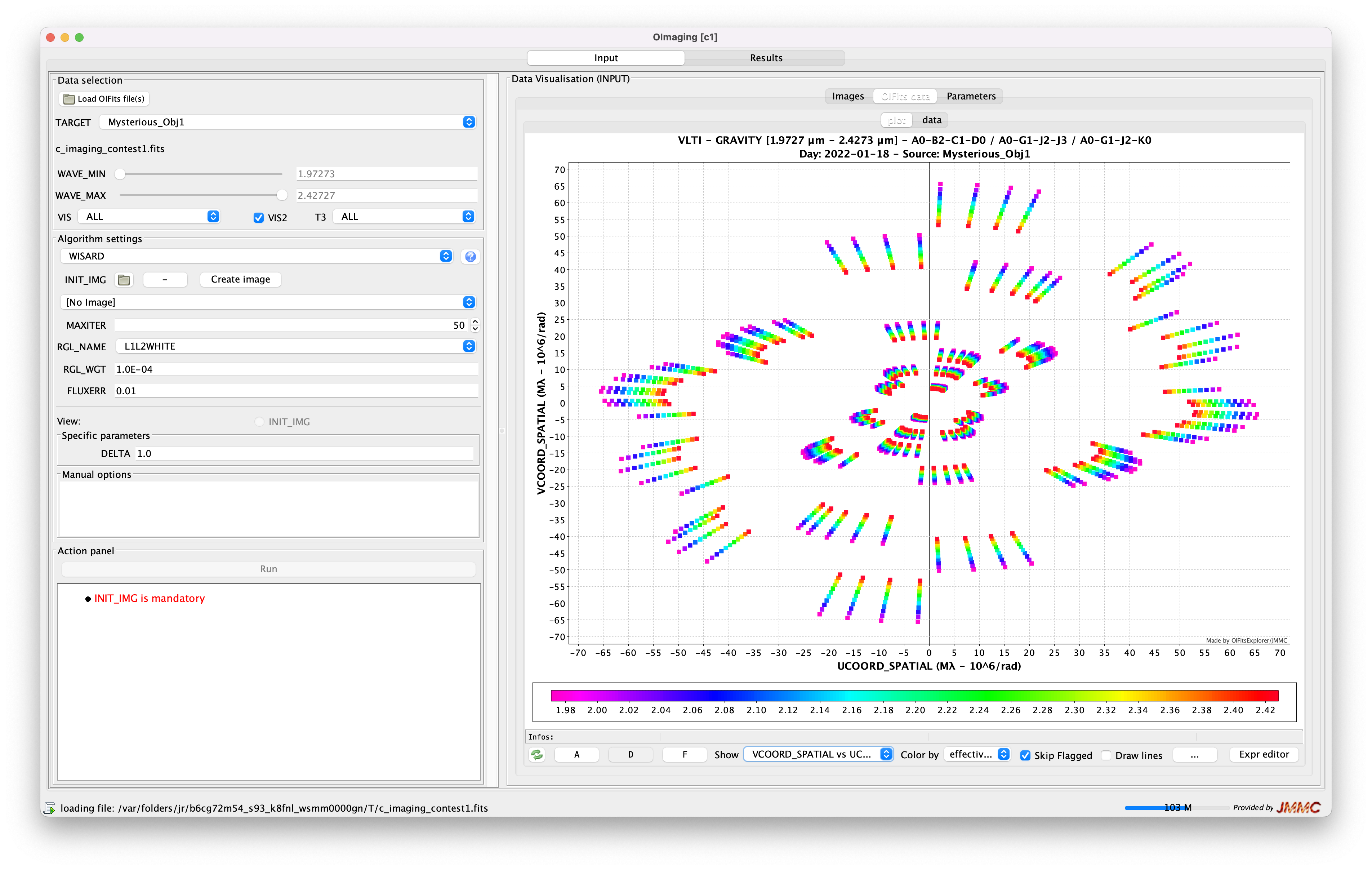
Figure 1: OImaging Input Panel

When started OImaging opens on the input panel that is used to load the data, select the algorithm and set the parameters.

3.1.1 OIFITS file loading

The data can be loaded either through the file loader or through the SAMP protocol [7]. This protocol is for sending data directly from one software program to another without saving it to a file. As an example, OIFITS files can be sent from the OIdb database [8] without explicitly saving them locally. If several files are selected they are just merged all together without any kind of filtering. When loading an OIFITS file, OImaging will check if it contains an ’IMAGE-OI INPUT PARAM’ HDU. If so, it will fill the fields of the input panel with the stored values. Otherwise, it will create it with default values.

3.1.2 Data visualization

Loaded data can be explored in the visualization sub-panel. In this sub-panel, the user can plot the data. He can also explore all the values stored in the OIFITS files: all the tables containing the data and in particular the values of the image reconstruction parameters stored in the ’IMAGE-OI INPUT PARAM’. This visualization sub-panel can also be used to display and modify all the images stored in the IMAGE-OI OIFITS file, in particular the initial image and the prior image.

3.1.3 Data selection

As explained above, any sophisticated selection, merging or editing of the data should be done by a separate tool such as JMMC’s OIFITSExplorer. However, basic selection tools are available in the input panel, namely the target and the wavelength range. In addition, the user can select the types of data used in the reconstruction from the amplitudes and the phases of the visibilities (VISAMP and VISPHI), the squared visibilities (VIS2) and the amplitudes and the phases of the bispectra (T3AMP and T3PHI).

3.1.4 Algorithm selection

The first step for performing image reconstruction is to select the algorithm. At the time of writing, four algorithms are available: WISARD[9], BSMEM[6], MiRA[10] and SPARCO[5]. For each algorithm a small help window can show a brief description, the reference paper and a description of all supported parameters.

3.1.5 Parameter settings

Once the algorithm has been selected, OImaging automatically updates the input fields used to set the parameters. There are three groups of parameters:

• first the parameters shared by all algorithms, namely the number of iterations MAXITER, the regularization name RGL_NAME, the regularization weight RGL_WGT and the error on the total flux FLUXERR;

• the second group contains parameters specific to the algorithm and/or the regularization function;

• in addition, there is a text field for Manual options that will be appended to the command line used to invoke the reconstruction software. This is a convenient way to access unsupported features that may change the algorithm behavior or the log contents. It is mainly intended for debugging.

3.1.6 Initial and prior images

All algorithms need an initial guess of the image. As explained in Sec. 2.2, the pixel size and the dimensions of the initial image determine those of the reconstructed image. This initial image can be specified by several means:

• loading a FITS file locally,

• sending the image from another software like SAO-DS9[11] or LITpro[12]. This is particularly convenient as an initial estimate of the target morphology can be done with the model fitting software LITpro. LITpro can then generate the modeled image and send it to OImaging as an initial guess;

• OImaging has a small widget accessible by the create image button to create an image of a Gaussian. Depending of the Gaussian width, it can approximate either a Dirac or a constant background. In this widget, OImaging suggests default sizes of both the field of view and the pixel according to the size of the telescope and the maximum baseline;

• after some reconstruction iterations, previous results can also be used as initial image; also

• any loaded image can be edited to change is pixel size or its field of view by the mean of the modify image button at the top right of the image.

Some regularization functions require a prior image, which can be viewed using the view radio-button next to the parameter field. By default, if no prior image is set, the initial image is also used as the prior image.

3.1.7 Running the algorithm

When all parameters are correctly set, the algorithm can be run by clicking on the Run button. This button stays grayed out when there is an issue with the parameters. In that case, the user must read the message in the box below it. A second click on the Run button while the reconstruction is in progress cancels the computation.

3.2 Result panel

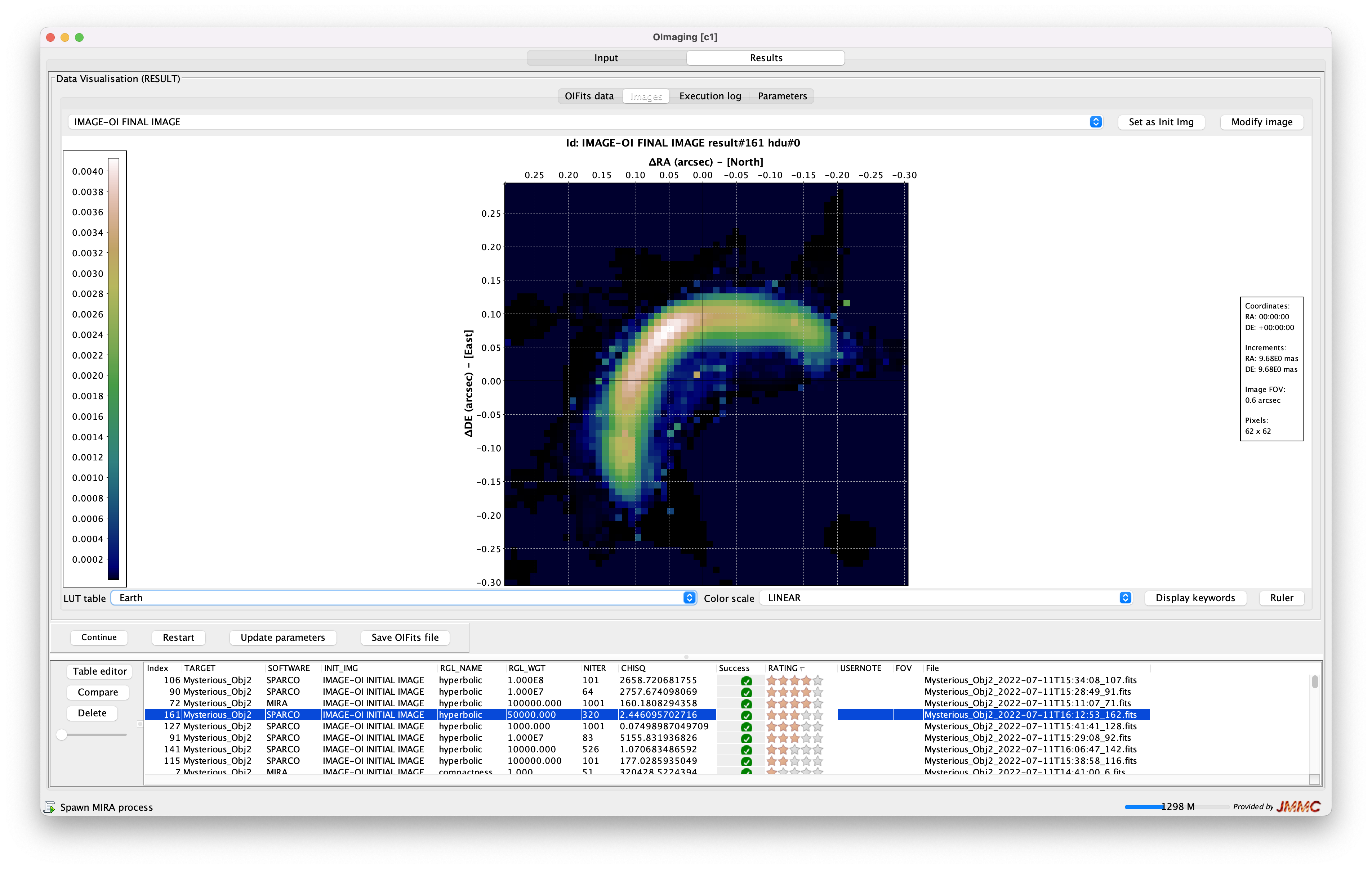
Figure 2: OImaging Result Panel

The reconstructed images are shown in the result panel. This panel is composed of two sub-panels: the visualization sub-panel and the results table.

3.2.1 Results table

All results are stored in the results table at the bottom of the result panel. This table gives an overview of all the parameters stored in the result OI-IMAGE OIFITS files: either the input parameters such as the algorithm or the regularization weight or the output parameters computed by the algorithm such as the $\chi^{2}$ or the value of the regularization function. The table contains additional fields such as “Success” that show if the software stopped with an error. It also contains RATING and USERNOTE fields to allow the user to add additional information concerning a given reconstruction. These fields are all stored in the resulting OIFITS file.

To help the user navigate the results, the table can be sorted and edited. Using the Table Editor button, the table is fully customizable: any keyword present in the OIFITS file can be set as field in the table. Reconstruction results can be also be removed from the table by means of the Delete button.

When several results are selected, the compare button displays the reconstructed images side by side.

3.2.2 Result visualization

The selected result in the panel can be explored in a visualization sub-panel similar to the visualization sub-panel of the input panel. This visualization sub-panel is itself composed of four sub-panels:

• OIFits data sub-panel shows all the data stored in the OI-FITS tables either as text or as graphs. As the algorithms store the model of the data as additional columns with the prefix ’NS_MODEL_’, the modeled data and the residuals can also be plotted in this panel.

• Images sub-panel can display all the images contained in the OI-FITS file, by default the result image but also the initial image or the prior image depending on the HDU name selected in the menu at the top of the panel. This Image sub-panel also has two buttons at the top: a Set as init img button that put the displayed image in the initial image list in the input panel and a modify image button to change the sizes of the pixels and the field of view. In that case, the modified image does not overwrite the current image but is rather put the initial image list in the input panel. This sub-panel contains also a ruler button to help the user to measure distance and angle on the image.

• Execution log sub-panel shows the output log of the algorithm.

• Parameters sub-panel shows the parameters set in the HDUs ’IMAGE-OI INPUT PARAM’ and
  ’IMAGE-OI OUTPUT PARAM’.

3.2.3 Interacting with the results

In addition to the visualization sub-panel and the results table, the result panel shows four buttons for interacting with the selected results:

• Continue uses the reconstructed image as the initial image to perform MAXITER more iterations without changing any other parameters. It is a convenient way to perform a reconstruction for a large number of iterations checking the image every MAXITER iterations.

• Restart updates all the parameters in the input panel with the values in ’IMAGE-OI OUTPUT PARAM’ and with the same initial image.

• Update parameters is equivalent to Restart but using the result image as the initial image in the input panel.

• Save OIFits files saves the selected result.

4 Conclusion

We have presented in this paper a new OI-FITS extension: IMAGE-OI. This new standard has two mains purpose: (i) to standardize communicating with image reconstruction software backends and (ii) to store in a single file along with the reconstructed image, the data and all the parameters that where used in the reconstruction process enabling its reproducibility.

In a second part, we presented presents OImaging, a graphical user interface that uses this standard to provide a common frontend for several image reconstruction algorithms. This open source software is freely available on JMMC website. Its development is still active and several feature may be added in the future (such that the automatic fit of a simple model to generate the initial image, tools to perform batch processing with different parameters). Support for this software is provided via the network of VLTI Expertise Centers and help can be requested at https://apps.jmmc.fr/feedback/.

References

- [1] Thiébaut, É. and Young, J., “Principles of image reconstruction in optical interferometry: tutorial,” JOSA A 34(6), 904–923 (2017).
- [2] Pauls, T. A., Young, J. S., Cotton, W. D., and Monnier, J. D., “A data exchange standard for optical (visible/IR) interferometry,” PASP 117, 1255–1262 (Nov. 2005).
- [3] Duvert, Gilles, Young, John, and Hummel, Christian A., “Oifits 2: the 2nd version of the data exchange standard for optical interferometry,” A&A 597, A8 (2017).
- [4] Pence, W. D., Chiappetti, L., Page, C. G., Shaw, R. A., and Stobie, E., “Definition of the Flexible Image Transport System (FITS), version 3.0,” A&A 524, A42 (Nov 2010).
- [5] Kluska, J., Malbet, F., Berger, J.-P., Baron, F., Lazareff, B., Le Bouquin, J.-B., Monnier, J., Soulez, F., and Thiébaut, E., “Sparco: a semi-parametric approach for image reconstruction of chromatic objects-application to young stellar objects,” Astronomy & Astrophysics 564, A80 (2014).
- [6] Baron, F. and Young, J. S., “Image reconstruction at cambridge university,” in [Optical and Infrared Interferometry ], 7013, 1288–1298, SPIE (2008).
- [7] Taylor, M. B., Boch, T., and Taylor, J., “Samp, the simple application messaging protocol: Letting applications talk to each other,” Astronomy and Computing 11, 81–90 (2015).
- [8] Haubois, X., Bernaud, P., Mella, G., Duvert, G., Benisty, M., Bério, P., Bourges, L., Chelli, A. E., Chesneau, O., Lacour, S., Lafrasse, S., Le Bouquin, J.-B., Mourard, D., Nardetto, N., and Olofsson, J., “A global database for optical interferometry,” in [Optical and Infrared Interferometry IV ], Rajagopal, J. K., Creech-Eakman, M. J., and Malbet, F., eds., Society of Photo-Optical Instrumentation Engineers (SPIE) Conference Series 9146, 91460O (July 2014).
- [9] Meimon, S. C., Mugnier, L. M., and Le Besnerais, G., “Reconstruction method for weak-phase optical interferometry,” Optics Letters 30(14), 1809–1811 (2005).
- [10] Thiébaut, E., “MIRA: an effective imaging algorithm for optical interferometry,” in [Optical and Infrared Interferometry ], Schöller, M., Danchi, W. C., and Delplancke, F., eds., 7013, 479 – 490, International Society for Optics and Photonics, SPIE (2008).
- [11] Joye, W. A. and Mandel, E., “New features of saoimage ds9,” in [Astronomical data analysis software and systems XII ], 295, 489 (2003).
- [12] Tallon-Bosc, I., Tallon, M., Thiébaut, E., Béchet, C., Mella, G., Lafrasse, S., Chesneau, O., de Souza, A. D., Duvert, G., Mourard, D., et al., “Litpro: a model fitting software for optical interferometry,” in [Optical and Infrared Interferometry ], 7013, 491–499, SPIE (2008).