Model-based gym environments for limit order book trading

Abstract.

Within the mathematical finance literature there is a rich catalogue of mathematical models for studying algorithmic trading problems – such as market-making and optimal execution – in limit order books. This paper introduces mbt_gym, a Python module that provides a suite of gym environments for training reinforcement learning (RL) agents to solve such model-based trading problems. The module is set up in an extensible way to allow the combination of different aspects of different models. It supports highly efficient implementations of vectorized environments to allow faster training of RL agents. In this paper, we motivate the challenge of using RL to solve such model-based limit order book problems in mathematical finance, we explain the design of our gym environment, and then demonstrate its use in solving standard and non-standard problems from the literature. Finally, we lay out a roadmap for further development of our module, which we provide as an open source repository on GitHub so that it can serve as a focal point for RL research in model-based algorithmic trading.

1. Introduction

A substantial proportion of financial markets use the limit order book (LOB) mechanism to match buyers and sellers (Gould et al., 2013). Consequently, LOBs have been a major object of study within mathematical finance. A wide range of mathematical models that capture price dynamics and order arrivals have been developed, and then trading problems, such as market making or optimal execution, have been analysed for these models. The models are differentiated primarily by the stochastic processes that drive the price and order dynamics, the actions available to the agent, and the agent’s reward function.

Typically these problems have been solved (often approximately) using standard methods from the theory of Partial Differential Equations (PDEs), namely by formulating the Hamilton-Jacobi-Bellman (HJB) equation and using Euler schemes or finite-difference methods to solve them numerically. However:

1. The numerical HJB approach requires solution schemes that are tailored to the particular stochastic processes of the model. Ideally, solution approaches would be more model agnostic.

2. The numerical HJB approach suffers particularly strongly from the curse of dimensionality, which has also constrained the types of models that have been considered and solved this way.

3. When employing the HJB approach, one often looks for semi-explicit solutions. For this reason, one considers ‘nice’ functions to define models, which constrains the range of trading problems that are considered in the literature.

   inline,color=purple!40,caption=]Martin: I am still not fully happy with (3) - the control being in feedback form always follows in the HJB approach. I would rather write something like this: When employing the HJB approach, one often looks for semi-explicit solutions. For this reason, one considers ’nice’ functions as model input, which constrains the range of trading problems that are considered in the literature.

Reinforcement Learning (RL) is an approach to solving control problems that is based on trial and error. It has seen very rapid development since the Deep Learning revolution, with a number of prominent success stories. We contend that using RL to solve model-based LOB trading problems is important and exciting:

• for mathematical finance by providing a complementary solution method in addition to PDE approaches that will enable the solution of richer and more realistic models; and

• for the RL community by providing a new class of problems on which to develop and understand different RL algorithms.

In relation to the highlighted weaknesses of the HJB approach, we note that by using model-free RL, one can in principle solve richer models with assumptions that do not suit the HJB approach well, use the same learning method across many models, and solve higher-dimensional and thereby richer models. We present an open-source benchmark module that implements a range of LOB models and trading problems from the mathematical finance literature, along with RL-based solution methods. Our goal is to showcase the potential of RL for solving these types of problems, and facilitate further research in this exciting direction.

While RL is very promising for solving these problems, RL does have a major accepted weakness of being very sample inefficient. Fortunately, the model-based trading problems that we study allow for highly efficient implementations of vectorized environments, which we leverage in our implementations, and we find that using this vectorization (essentially parallelization) is crucial to get close-to-optimal solutions to the benchmark problems that we study.

Our main contributions.

• We provide an open source repository of unified gym environments for a range of model-based LOB trading problems.

• We provide optimal baseline agents so that one can benchmark the performance of RL algorithms.

• A key strength of our implementations is the modular design that supports picking and choosing different components of existing models, for example using a reward function from one model, with the prices and execution processes from another.

• We have connected our environments to Stable Baselines 3 (SB3), which provides a suite of state-of-the-art RL algorithms. These algorithms perform robustly across a variety of tasks, allowing a “plug-and-play” approach to training RL agents on previously unstudied problems. We demonstrate its use by quickly solving a popular market making problem to near optimality using proximal policy optimisation (Schulman et al., 2017), showing the benefit of our custom highly-efficient vectorized environments.

• Going further, we lay out a roadmap for further developments of our RL for model-based trading benchmark suite, both in terms of the models and trading problems and in terms of the RL algorithms used to find solutions.

The module is available at: https://github.com/JJJerome/mbt_gym.

1.1. Literature review

1.1.1. Mathematical finance

The market-making problem with limit orders was first introduced in (Ho and Stoll, 1981) and mathematically formalized three decades later by (Avellaneda and Stoikov, 2008). From that point on, a large volume of research has been produced by the mathematical finance community. The work of (Guéant et al., 2013) presents an explicit solution to the market making problem with inventory constraints. Examples of subsequent developments featuring more realistic models are those by (Guilbaud and Pham, 2013; Cartea et al., 2014). Other relevant extensions include the works of (Cartea et al., 2018; Cartea and Wang, 2020) where signals are incorporated into the framework for both continuous action spaces and binary actions. The community continues to work on aspects of the market making problem, from options (Baldacci et al., 2021) and foreign exchange (Barzykin et al., 2022) to automated market making (Cartea et al., 2022).

Similar to the market making case, the optimal execution literature is vast; starting with (Bertsimas and Lo, 1998; Almgren and Chriss, 2001), the problem has attracted increasing attention. A significant focus of model design is on how the market processes the order flow from the liquidator (and other market participants), and how signals can be constructed and exploited (Cartea and Jaimungal, 2016, 2015; Gatheral et al., 2012; Forde et al., 2022; Neuman and Voß, 2022; Donnelly and Lorig, 2020; Kalsi et al., 2020; Cartea et al., 2020). Further investigations include the case of stochastic volatility and liquidity (Almgren, 2012), stochastic price impact (Barger and Lorig, 2019; Fouque et al., 2022), and latency and related frictions (Moallemi and Sağlam, 2013; Cartea and Sánchez-Betancourt, 2021).

See (Cartea et al., 2015; Gueant, 2016) for an excellent textbook treatment of both optimal execution and market making.

1.1.2. Reinforcement learning for high-frequency trading literature

The following section provides a brief summary of the reinforcement learning for high-frequency trading literature, paying particular attention to the dynamics of the learning environment since that is the main focus of this paper. This section also mainly focuses on the market-making problem as opposed to the optimal execution problem since the majority of the environments currently provided in mbt_gym focus on market-making, however, a brief summary of the RL for optimal execution literature is also included.

There are broadly three main approaches to modelling the market dynamics for a reinforcement learning environment. The first is to use a “market replay” approach, in which historical data is replayed in a simulator, and the learning agent interacts with it. The second is model-based approaches, a category in which this paper sits. The final approach is that of agent-based market simulators in which hand-crafted agents that aim to model real-life market participants are allowed to interact with each other and the training agent through an exchange mechanism. A good summary of the merits of each approach is provided in Balch et al. (2019).

Papers on high-frequency trading which train agents using a market replay simulator include: Nevmyvaka et al. (2006) and Jerome et al. (2022), which use Nasdaq data; Spooner et al. (2018) which uses data from LSE; Zhong et al. (2020) which uses futures data from CME; Xu et al. (2022), which uses data from XSHE; and Patel (2018), Sadighian (2019) and Gasperov and Kostanjcar (2021), which uses cryptocurrency data.

Some notable papers that consider the market-making problem in a model-based environment include: Chan and Shelton (2001), which uses a Poisson-process-driven model similar to Glosten and Milgrom (1985); Kim and Shelton (2002), who fit a hidden Markov model to Nasdaq trade data; Lim and Gorse (2018), which considers the market making problem in the Poisson-process-driven model of Cont et al. (2010); and Spooner and Savani (2020), which considers a robust adversarial version of the problem in (Cartea et al., 2015, Section 10.2).

Finally, agent-based high-frequency trading simulators are used to train RL agents in Ganesh et al. (2019), Kumar (2020), Karpe et al. (2020) and Amrouni et al. (2021).

2. Design of the module

Our module has been designed with the following principles in mind. The code should be extensible and general and minimize code duplication. For example, all our gym environments inherit from a class TradingEnvironment and use the same following shared step and “update” functions. The step function, shown below, is not specific to the trading problem.

⬇

from typing import Union, Tuple

import gym

import numpy as np

from gym.spaces import Box

from DRL4AMM.stochastic_processes.arrival_models import ArrivalModel, PoissonArrivalModel

from DRL4AMM.stochastic_processes.fill_probability_models import FillProbabilityModel, ExponentialFillFunction

from DRL4AMM.stochastic_processes.midprice_models import MidpriceModel, BrownianMotionMidpriceModel

from DRL4AMM.gym.tracking.InfoCalculator import InfoCalculator, ActionInfoCalculator

from DRL4AMM.rewards.RewardFunctions import RewardFunction, PnL

ACTION_SPACES = [”touch”, ”limit”, ”limit_and_market”]

CASH_INDEX = 0

INVENTORY_INDEX = 1

TIME_INDEX = 2

ASSET_PRICE_INDEX = 3

class TradingEnvironment(gym.Env):

metadata = {”render.modes”: [”human”]}

def __init__(

self,

terminal_time: float = 1.0,

n_steps: int = 20 * 10,

reward_function: RewardFunction = None,

midprice_model: MidpriceModel = None,

arrival_model: ArrivalModel = None,

fill_probability_model: FillProbabilityModel = None,

action_type: str = ”limit”,

initial_cash: float = 0.0,

initial_inventory: Union[int, Tuple[float, float]] = 0, # Either a deterministic initial inventory, or a tuple

max_inventory: int = 10_000, # representing the mean and variance of it.

max_cash: float = None,

max_stock_price: float = None,

max_depth: float = None,

half_spread: float = None,

info_calculator: InfoCalculator = None,

seed: int = None,

num_trajectories: int = 1,

):

super(TradingEnvironment, self).__init__()

self.terminal_time = terminal_time

self.num_trajectories = num_trajectories

self.n_steps = n_steps

self.step_size = self.terminal_time / self.n_steps

self.reward_function = reward_function or PnL()

self.midprice_model: MidpriceModel = midprice_model or BrownianMotionMidpriceModel(

step_size=self.step_size, num_trajectories=num_trajectories

)

self.arrival_model: ArrivalModel = arrival_model or PoissonArrivalModel(

step_size=self.step_size, num_trajectories=num_trajectories

)

self.fill_probability_model: FillProbabilityModel = fill_probability_model or ExponentialFillFunction(

step_size=self.step_size, num_trajectories=num_trajectories

)

self.action_type = action_type

self.rng = np.random.default_rng(seed)

self.initial_cash = initial_cash

self.initial_inventory = initial_inventory

self.max_inventory = max_inventory

self.state = self.initial_state

self.max_stock_price = max_stock_price or self.midprice_model.max_value[0, 0]

self.max_cash = max_cash or self._get_max_cash()

self.max_depth = max_depth or self.fill_probability_model.max_depth

self.observation_space = self._get_observation_space()

self.action_space = self._get_action_space()

self.half_spread = half_spread

self.info_calculator = info_calculator or ActionInfoCalculator()

self.midprice_index_range = self._get_midprice_index_range()

self.arrival_index_range = self._get_fill_index_range()

self.fill_index_range = self._get_fill_index_range()

self._check_params()

self.empty_infos = [{} for _ in range(self.num_trajectories)]

ones = np.ones((self.num_trajectories, 1))

self.multiplier = np.append(-ones, ones, axis=1)

def reset(self):

self.midprice_model.reset()

self.arrival_model.reset()

self.fill_probability_model.reset()

self.state = self.initial_state

return self.state.copy()

def step(self, action: np.ndarray):

current_state = self.state.copy()

next_state = self._update_state(action)

done = self.state[0, 2] >= self.terminal_time - self.step_size / 2

dones = np.full((self.num_trajectories,), done, dtype=bool)

rewards = self.reward_function.calculate(current_state, action,

next_state, done)

infos = self.empty_infos

return self.state.copy(), rewards, dones, infos

def _get_max_cash(self) -> float:

return self.max_inventory * self.max_stock_price

# action = [bid_depth, ask_depth, MO_buy, MO_sell]

# state[0]=cash, state[1]=inventory, state[2]=time, state[3] = asset_price, and then remaining states depend on

# the dimensionality of the arrival process, the midprice process and the fill probability process.

def _update_state(self, action: np.ndarray) -> np.ndarray:

arrivals = self.arrival_model.get_arrivals()

if self.action_type in [”limit”, ”limit_and_market”]:

depths = self.limit_depths(action)

fills = self.fill_probability_model.get_fills(depths)

else:

fills = self.post_at_touch(action)

self._update_agent_state(arrivals, fills, action)

self._update_market_state(arrivals, fills, action)

return self.state

def _update_market_state(self, arrivals, fills, action):

self.arrival_model.update(arrivals, fills, action)

self.midprice_model.update(arrivals, fills, action)

self.fill_probability_model.update(arrivals, fills, action)

self.state[:, self.midprice_index_range[0]:

self.midprice_index_range[1]] =

self.midprice_model.current_state

self.state[:, self.arrival_index_range[0]:

self.arrival_index_range[1]] =

self.arrival_model.current_state

self.state[:, self.fill_index_range[0]:

self.fill_index_range[1]] =

self.fill_probability_model.current_state

def _update_agent_state(self, arrivals: np.ndarray, fills: np.ndarray,

action: np.ndarray):

if self.action_type == ”limit_and_market”:

mo_buy = np.single(self.market_order_buy(action) > 0.5)

mo_sell = np.single(self.market_order_sell(action) > 0.5)

best_bid = self.midprice - self.half_spread

best_ask = self.midprice + self.half_spread

self.state[:, CASH_INDEX] += mo_sell * best_bid - mo_buy * best_ask

self.state[:, INVENTORY_INDEX] += mo_buy - mo_sell

self.state[:, INVENTORY_INDEX] +=

np.sum(arrivals * fills * -self.multiplier, axis=1)

if self.action_type == ”touch”:

self.state[:, CASH_INDEX] += np.sum(

self.multiplier * arrivals * fills *\

(self.midprice + self.half_spread * self.multiplier), axis=1)

else:

self.state[:, CASH_INDEX] += np.sum(

self.multiplier * arrivals * fills *\

(self.midprice + self.limit_depths(action) * self.multiplier),

axis=1)

self._clip_inventory_and_cash()

self.state[:, TIME_INDEX] += self.step_size

@property

def midprice(self):

return self.midprice_model.current_state[:, 0].reshape(-1, 1)

def _clip_inventory_and_cash(self):

self.state[:, 1] = self._clip(self.state[:, 1], -self.max_inventory, self.max_inventory, cash_flag=False)

self.state[:, 0] = self._clip(self.state[:, 0], -self.max_cash, self.max_cash, cash_flag=True)

def _clip(self, not_clipped: float, min: float, max: float, cash_flag: bool) -> float:

clipped = np.clip(not_clipped, min, max)

if (not_clipped != clipped).any() and cash_flag:

print(f”Clipping agent’s cash from {not_clipped} to {clipped}.”)

if (not_clipped != clipped).any() and ~cash_flag:

print(f”Clipping agent’s inventory from {not_clipped} to {clipped}.”)

return clipped

def limit_depths(self, action: np.ndarray):

if self.action_type in [”limit”, ”limit_and_market”]:

return action[:, 0:2]

else:

raise Exception(’Bid depth only exists for action_type in [”limit”, ”limit_and_market”].’)

def market_order_buy(self, action: np.ndarray):

if self.action_type == ”limit_and_market”:

return action[:, 2]

else:

raise Exception(’Market order buy action only exists for action_type == ”limit_and_market”.’)

def market_order_sell(self, action: np.ndarray):

if self.action_type == ”limit_and_market”:

return action[:, 3]

else:

raise Exception(’Market order sell action only exists for action_type == ”limit_and_market”.’)

def post_at_touch(self, action: np.ndarray):

if self.action_type == ”touch”:

return action[:, 0:2]

else:

raise Exception(’Post buy at touch action only exists for action_type == ”touch”.’)

@property

def initial_state(self) -> np.ndarray:

scalar_initial_state = np.array([[self.initial_cash, 0, 0.0]])

initial_state = np.repeat(scalar_initial_state, self.num_trajectories, axis=0)

if isinstance(self.initial_inventory, tuple) and len(self.initial_inventory) == 2:

# initial_inventories = self.rng.normal(*self.initial_inventory, size=self.num_trajectories).round()

initial_inventories = self.rng.integers(*self.initial_inventory, size=self.num_trajectories)

elif isinstance(self.initial_inventory, int):

initial_inventories = self.initial_inventory * np.ones((self.num_trajectories,))

else:

raise Exception(”Initial inventory must be a tuple of length 2 or an int.”)

initial_state[:, 1] = initial_inventories

initial_state = np.append(initial_state, self.midprice_model.initial_vector_state, axis=1)

initial_state = np.append(initial_state, self.arrival_model.initial_vector_state, axis=1)

initial_state = np.append(initial_state, self.fill_probability_model.initial_vector_state, axis=1)

return initial_state

def _get_current_state(self) -> np.ndarray:

state = self.state[:, 0:3]

state = np.append(state, self.midprice_model.current_state, axis=1)

state = np.append(state, self.arrival_model.current_state, axis=1)

state = np.append(state, self.fill_probability_model.current_state, axis=1)

return state

def _get_observation_space(self) -> gym.spaces.Space:

”””The observation space consists of a numpy array containg the agent’s cash, the agent’s inventory and the

current time. It also contains the states of the arrival model, the midprice model and the fill probability

model in that order.”””

low = np.array([-self.max_cash, -self.max_inventory, 0])

low = np.append(low, self.arrival_model.min_value)

low = np.append(low, self.midprice_model.min_value)

low = np.append(low, self.fill_probability_model.min_value)

high = np.array([self.max_cash, self.max_inventory, self.terminal_time])

high = np.append(high, self.arrival_model.max_value)

high = np.append(high, self.midprice_model.max_value)

high = np.append(high, self.fill_probability_model.max_value)

return Box(

low=low,

high=high,

dtype=np.float64,

)

def _get_action_space(self) -> gym.spaces.Space:

assert self.action_type in ACTION_SPACES, f”Action type {self.action_type} is not in {ACTION_SPACES}.”

if self.action_type == ”touch”:

return gym.spaces.MultiBinary(2) # agent chooses spread on bid and ask

if self.action_type == ”limit”:

return gym.spaces.Box(low=0.0, high=self.max_depth, shape=(2,)) # agent chooses spread on bid and ask

if self.action_type == ”limit_and_market”:

return gym.spaces.Box(

low=np.zeros(

4,

),

high=np.array(self.max_depth, self.max_depth, 1, 1),

shape=(2,),

)

def _get_midprice_index_range(self):

min_midprice_index = 3

max_midprice_index = 3 + self.midprice_model.initial_vector_state.shape[1]

return min_midprice_index, max_midprice_index

def _get_arrival_index_range(self):

min_arrival_index = self._get_midprice_index_range()[1]

max_arrival_index = self._get_midprice_index_range()[1] + self.arrival_model.initial_vector_state.shape[1]

return min_arrival_index, max_arrival_index

def _get_fill_index_range(self):

min_fill_index = self._get_arrival_index_range()[1]

max_fill_index = self._get_arrival_index_range()[1] + self.fill_probability_model.initial_vector_state.shape[1]

return min_fill_index, max_fill_index

@staticmethod

def _get_max_depth():

return 4.0 # TODO: improve

@staticmethod

def _clamp(probability):

return max(min(probability, 1), 0)

def _check_params(self):

assert self.action_type in [”limit”, ”limit_and_market”, ”touch”]

for stochastic_process in [self.midprice_model, self.arrival_model, self.fill_probability_model]:

assert np.isclose(stochastic_process.step_size, self.step_size, 2), (

f”{type(self.midprice_model).__name__}.step_size = {stochastic_process.step_size}, ”

+ f” but env.step_size = {self.terminal_time/self.n_steps}”

)

_update_state, shown next, is specific to the trading problem.

⬇

from typing import Union, Tuple

import gym

import numpy as np

from gym.spaces import Box

from DRL4AMM.stochastic_processes.arrival_models import ArrivalModel, PoissonArrivalModel

from DRL4AMM.stochastic_processes.fill_probability_models import FillProbabilityModel, ExponentialFillFunction

from DRL4AMM.stochastic_processes.midprice_models import MidpriceModel, BrownianMotionMidpriceModel

from DRL4AMM.gym.tracking.InfoCalculator import InfoCalculator, ActionInfoCalculator

from DRL4AMM.rewards.RewardFunctions import RewardFunction, PnL

ACTION_SPACES = [”touch”, ”limit”, ”limit_and_market”]

CASH_INDEX = 0

INVENTORY_INDEX = 1

TIME_INDEX = 2

ASSET_PRICE_INDEX = 3

class TradingEnvironment(gym.Env):

metadata = {”render.modes”: [”human”]}

def __init__(

self,

terminal_time: float = 1.0,

n_steps: int = 20 * 10,

reward_function: RewardFunction = None,

midprice_model: MidpriceModel = None,

arrival_model: ArrivalModel = None,

fill_probability_model: FillProbabilityModel = None,

action_type: str = ”limit”,

initial_cash: float = 0.0,

initial_inventory: Union[int, Tuple[float, float]] = 0, # Either a deterministic initial inventory, or a tuple

max_inventory: int = 10_000, # representing the mean and variance of it.

max_cash: float = None,

max_stock_price: float = None,

max_depth: float = None,

half_spread: float = None,

info_calculator: InfoCalculator = None,

seed: int = None,

num_trajectories: int = 1,

):

super(TradingEnvironment, self).__init__()

self.terminal_time = terminal_time

self.num_trajectories = num_trajectories

self.n_steps = n_steps

self.step_size = self.terminal_time / self.n_steps

self.reward_function = reward_function or PnL()

self.midprice_model: MidpriceModel = midprice_model or BrownianMotionMidpriceModel(

step_size=self.step_size, num_trajectories=num_trajectories

)

self.arrival_model: ArrivalModel = arrival_model or PoissonArrivalModel(

step_size=self.step_size, num_trajectories=num_trajectories

)

self.fill_probability_model: FillProbabilityModel = fill_probability_model or ExponentialFillFunction(

step_size=self.step_size, num_trajectories=num_trajectories

)

self.action_type = action_type

self.rng = np.random.default_rng(seed)

self.initial_cash = initial_cash

self.initial_inventory = initial_inventory

self.max_inventory = max_inventory

self.state = self.initial_state

self.max_stock_price = max_stock_price or self.midprice_model.max_value[0, 0]

self.max_cash = max_cash or self._get_max_cash()

self.max_depth = max_depth or self.fill_probability_model.max_depth

self.observation_space = self._get_observation_space()

self.action_space = self._get_action_space()

self.half_spread = half_spread

self.info_calculator = info_calculator or ActionInfoCalculator()

self.midprice_index_range = self._get_midprice_index_range()

self.arrival_index_range = self._get_fill_index_range()

self.fill_index_range = self._get_fill_index_range()

self._check_params()

self.empty_infos = [{} for _ in range(self.num_trajectories)]

ones = np.ones((self.num_trajectories, 1))

self.multiplier = np.append(-ones, ones, axis=1)

def reset(self):

self.midprice_model.reset()

self.arrival_model.reset()

self.fill_probability_model.reset()

self.state = self.initial_state

return self.state.copy()

def step(self, action: np.ndarray):

current_state = self.state.copy()

next_state = self._update_state(action)

done = self.state[0, 2] >= self.terminal_time - self.step_size / 2

dones = np.full((self.num_trajectories,), done, dtype=bool)

rewards = self.reward_function.calculate(current_state, action,

next_state, done)

infos = self.empty_infos

return self.state.copy(), rewards, dones, infos

def _get_max_cash(self) -> float:

return self.max_inventory * self.max_stock_price

# action = [bid_depth, ask_depth, MO_buy, MO_sell]

# state[0]=cash, state[1]=inventory, state[2]=time, state[3] = asset_price, and then remaining states depend on

# the dimensionality of the arrival process, the midprice process and the fill probability process.

def _update_state(self, action: np.ndarray) -> np.ndarray:

arrivals = self.arrival_model.get_arrivals()

if self.action_type in [”limit”, ”limit_and_market”]:

depths = self.limit_depths(action)

fills = self.fill_probability_model.get_fills(depths)

else:

fills = self.post_at_touch(action)

self._update_agent_state(arrivals, fills, action)

self._update_market_state(arrivals, fills, action)

return self.state

def _update_market_state(self, arrivals, fills, action):

self.arrival_model.update(arrivals, fills, action)

self.midprice_model.update(arrivals, fills, action)

self.fill_probability_model.update(arrivals, fills, action)

self.state[:, self.midprice_index_range[0]:

self.midprice_index_range[1]] =

self.midprice_model.current_state

self.state[:, self.arrival_index_range[0]:

self.arrival_index_range[1]] =

self.arrival_model.current_state

self.state[:, self.fill_index_range[0]:

self.fill_index_range[1]] =

self.fill_probability_model.current_state

def _update_agent_state(self, arrivals: np.ndarray, fills: np.ndarray,

action: np.ndarray):

if self.action_type == ”limit_and_market”:

mo_buy = np.single(self.market_order_buy(action) > 0.5)

mo_sell = np.single(self.market_order_sell(action) > 0.5)

best_bid = self.midprice - self.half_spread

best_ask = self.midprice + self.half_spread

self.state[:, CASH_INDEX] += mo_sell * best_bid - mo_buy * best_ask

self.state[:, INVENTORY_INDEX] += mo_buy - mo_sell

self.state[:, INVENTORY_INDEX] +=

np.sum(arrivals * fills * -self.multiplier, axis=1)

if self.action_type == ”touch”:

self.state[:, CASH_INDEX] += np.sum(

self.multiplier * arrivals * fills *\

(self.midprice + self.half_spread * self.multiplier), axis=1)

else:

self.state[:, CASH_INDEX] += np.sum(

self.multiplier * arrivals * fills *\

(self.midprice + self.limit_depths(action) * self.multiplier),

axis=1)

self._clip_inventory_and_cash()

self.state[:, TIME_INDEX] += self.step_size

@property

def midprice(self):

return self.midprice_model.current_state[:, 0].reshape(-1, 1)

def _clip_inventory_and_cash(self):

self.state[:, 1] = self._clip(self.state[:, 1], -self.max_inventory, self.max_inventory, cash_flag=False)

self.state[:, 0] = self._clip(self.state[:, 0], -self.max_cash, self.max_cash, cash_flag=True)

def _clip(self, not_clipped: float, min: float, max: float, cash_flag: bool) -> float:

clipped = np.clip(not_clipped, min, max)

if (not_clipped != clipped).any() and cash_flag:

print(f”Clipping agent’s cash from {not_clipped} to {clipped}.”)

if (not_clipped != clipped).any() and ~cash_flag:

print(f”Clipping agent’s inventory from {not_clipped} to {clipped}.”)

return clipped

def limit_depths(self, action: np.ndarray):

if self.action_type in [”limit”, ”limit_and_market”]:

return action[:, 0:2]

else:

raise Exception(’Bid depth only exists for action_type in [”limit”, ”limit_and_market”].’)

def market_order_buy(self, action: np.ndarray):

if self.action_type == ”limit_and_market”:

return action[:, 2]

else:

raise Exception(’Market order buy action only exists for action_type == ”limit_and_market”.’)

def market_order_sell(self, action: np.ndarray):

if self.action_type == ”limit_and_market”:

return action[:, 3]

else:

raise Exception(’Market order sell action only exists for action_type == ”limit_and_market”.’)

def post_at_touch(self, action: np.ndarray):

if self.action_type == ”touch”:

return action[:, 0:2]

else:

raise Exception(’Post buy at touch action only exists for action_type == ”touch”.’)

@property

def initial_state(self) -> np.ndarray:

scalar_initial_state = np.array([[self.initial_cash, 0, 0.0]])

initial_state = np.repeat(scalar_initial_state, self.num_trajectories, axis=0)

if isinstance(self.initial_inventory, tuple) and len(self.initial_inventory) == 2:

# initial_inventories = self.rng.normal(*self.initial_inventory, size=self.num_trajectories).round()

initial_inventories = self.rng.integers(*self.initial_inventory, size=self.num_trajectories)

elif isinstance(self.initial_inventory, int):

initial_inventories = self.initial_inventory * np.ones((self.num_trajectories,))

else:

raise Exception(”Initial inventory must be a tuple of length 2 or an int.”)

initial_state[:, 1] = initial_inventories

initial_state = np.append(initial_state, self.midprice_model.initial_vector_state, axis=1)

initial_state = np.append(initial_state, self.arrival_model.initial_vector_state, axis=1)

initial_state = np.append(initial_state, self.fill_probability_model.initial_vector_state, axis=1)

return initial_state

def _get_current_state(self) -> np.ndarray:

state = self.state[:, 0:3]

state = np.append(state, self.midprice_model.current_state, axis=1)

state = np.append(state, self.arrival_model.current_state, axis=1)

state = np.append(state, self.fill_probability_model.current_state, axis=1)

return state

def _get_observation_space(self) -> gym.spaces.Space:

”””The observation space consists of a numpy array containg the agent’s cash, the agent’s inventory and the

current time. It also contains the states of the arrival model, the midprice model and the fill probability

model in that order.”””

low = np.array([-self.max_cash, -self.max_inventory, 0])

low = np.append(low, self.arrival_model.min_value)

low = np.append(low, self.midprice_model.min_value)

low = np.append(low, self.fill_probability_model.min_value)

high = np.array([self.max_cash, self.max_inventory, self.terminal_time])

high = np.append(high, self.arrival_model.max_value)

high = np.append(high, self.midprice_model.max_value)

high = np.append(high, self.fill_probability_model.max_value)

return Box(

low=low,

high=high,

dtype=np.float64,

)

def _get_action_space(self) -> gym.spaces.Space:

assert self.action_type in ACTION_SPACES, f”Action type {self.action_type} is not in {ACTION_SPACES}.”

if self.action_type == ”touch”:

return gym.spaces.MultiBinary(2) # agent chooses spread on bid and ask

if self.action_type == ”limit”:

return gym.spaces.Box(low=0.0, high=self.max_depth, shape=(2,)) # agent chooses spread on bid and ask

if self.action_type == ”limit_and_market”:

return gym.spaces.Box(

low=np.zeros(

4,

),

high=np.array(self.max_depth, self.max_depth, 1, 1),

shape=(2,),

)

def _get_midprice_index_range(self):

min_midprice_index = 3

max_midprice_index = 3 + self.midprice_model.initial_vector_state.shape[1]

return min_midprice_index, max_midprice_index

def _get_arrival_index_range(self):

min_arrival_index = self._get_midprice_index_range()[1]

max_arrival_index = self._get_midprice_index_range()[1] + self.arrival_model.initial_vector_state.shape[1]

return min_arrival_index, max_arrival_index

def _get_fill_index_range(self):

min_fill_index = self._get_arrival_index_range()[1]

max_fill_index = self._get_arrival_index_range()[1] + self.fill_probability_model.initial_vector_state.shape[1]

return min_fill_index, max_fill_index

@staticmethod

def _get_max_depth():

return 4.0 # TODO: improve

@staticmethod

def _clamp(probability):

return max(min(probability, 1), 0)

def _check_params(self):

assert self.action_type in [”limit”, ”limit_and_market”, ”touch”]

for stochastic_process in [self.midprice_model, self.arrival_model, self.fill_probability_model]:

assert np.isclose(stochastic_process.step_size, self.step_size, 2), (

f”{type(self.midprice_model).__name__}.step_size = {stochastic_process.step_size}, ”

+ f” but env.step_size = {self.terminal_time/self.n_steps}”

)

We are able to use a single _update_state function across many standard LOB trading models from the literature because they all share the same high-level dependency order between the different stochastic processes. In particular, this means that we can use a fixed sequence for computing the next step in these stochastic processes, with the order arrivals process updating first and then driving the mid-price process and then the fill probability model. The function _update_market_state, shown next, deals with simulating these.

⬇

from typing import Union, Tuple

import gym

import numpy as np

from gym.spaces import Box

from DRL4AMM.stochastic_processes.arrival_models import ArrivalModel, PoissonArrivalModel

from DRL4AMM.stochastic_processes.fill_probability_models import FillProbabilityModel, ExponentialFillFunction

from DRL4AMM.stochastic_processes.midprice_models import MidpriceModel, BrownianMotionMidpriceModel

from DRL4AMM.gym.tracking.InfoCalculator import InfoCalculator, ActionInfoCalculator

from DRL4AMM.rewards.RewardFunctions import RewardFunction, PnL

ACTION_SPACES = [”touch”, ”limit”, ”limit_and_market”]

CASH_INDEX = 0

INVENTORY_INDEX = 1

TIME_INDEX = 2

ASSET_PRICE_INDEX = 3

class TradingEnvironment(gym.Env):

metadata = {”render.modes”: [”human”]}

def __init__(

self,

terminal_time: float = 1.0,

n_steps: int = 20 * 10,

reward_function: RewardFunction = None,

midprice_model: MidpriceModel = None,

arrival_model: ArrivalModel = None,

fill_probability_model: FillProbabilityModel = None,

action_type: str = ”limit”,

initial_cash: float = 0.0,

initial_inventory: Union[int, Tuple[float, float]] = 0, # Either a deterministic initial inventory, or a tuple

max_inventory: int = 10_000, # representing the mean and variance of it.

max_cash: float = None,

max_stock_price: float = None,

max_depth: float = None,

half_spread: float = None,

info_calculator: InfoCalculator = None,

seed: int = None,

num_trajectories: int = 1,

):

super(TradingEnvironment, self).__init__()

self.terminal_time = terminal_time

self.num_trajectories = num_trajectories

self.n_steps = n_steps

self.step_size = self.terminal_time / self.n_steps

self.reward_function = reward_function or PnL()

self.midprice_model: MidpriceModel = midprice_model or BrownianMotionMidpriceModel(

step_size=self.step_size, num_trajectories=num_trajectories

)

self.arrival_model: ArrivalModel = arrival_model or PoissonArrivalModel(

step_size=self.step_size, num_trajectories=num_trajectories

)

self.fill_probability_model: FillProbabilityModel = fill_probability_model or ExponentialFillFunction(

step_size=self.step_size, num_trajectories=num_trajectories

)

self.action_type = action_type

self.rng = np.random.default_rng(seed)

self.initial_cash = initial_cash

self.initial_inventory = initial_inventory

self.max_inventory = max_inventory

self.state = self.initial_state

self.max_stock_price = max_stock_price or self.midprice_model.max_value[0, 0]

self.max_cash = max_cash or self._get_max_cash()

self.max_depth = max_depth or self.fill_probability_model.max_depth

self.observation_space = self._get_observation_space()

self.action_space = self._get_action_space()

self.half_spread = half_spread

self.info_calculator = info_calculator or ActionInfoCalculator()

self.midprice_index_range = self._get_midprice_index_range()

self.arrival_index_range = self._get_fill_index_range()

self.fill_index_range = self._get_fill_index_range()

self._check_params()

self.empty_infos = [{} for _ in range(self.num_trajectories)]

ones = np.ones((self.num_trajectories, 1))

self.multiplier = np.append(-ones, ones, axis=1)

def reset(self):

self.midprice_model.reset()

self.arrival_model.reset()

self.fill_probability_model.reset()

self.state = self.initial_state

return self.state.copy()

def step(self, action: np.ndarray):

current_state = self.state.copy()

next_state = self._update_state(action)

done = self.state[0, 2] >= self.terminal_time - self.step_size / 2

dones = np.full((self.num_trajectories,), done, dtype=bool)

rewards = self.reward_function.calculate(current_state, action,

next_state, done)

infos = self.empty_infos

return self.state.copy(), rewards, dones, infos

def _get_max_cash(self) -> float:

return self.max_inventory * self.max_stock_price

# action = [bid_depth, ask_depth, MO_buy, MO_sell]

# state[0]=cash, state[1]=inventory, state[2]=time, state[3] = asset_price, and then remaining states depend on

# the dimensionality of the arrival process, the midprice process and the fill probability process.

def _update_state(self, action: np.ndarray) -> np.ndarray:

arrivals = self.arrival_model.get_arrivals()

if self.action_type in [”limit”, ”limit_and_market”]:

depths = self.limit_depths(action)

fills = self.fill_probability_model.get_fills(depths)

else:

fills = self.post_at_touch(action)

self._update_agent_state(arrivals, fills, action)

self._update_market_state(arrivals, fills, action)

return self.state

def _update_market_state(self, arrivals, fills, action):

self.arrival_model.update(arrivals, fills, action)

self.midprice_model.update(arrivals, fills, action)

self.fill_probability_model.update(arrivals, fills, action)

self.state[:, self.midprice_index_range[0]:

self.midprice_index_range[1]] =

self.midprice_model.current_state

self.state[:, self.arrival_index_range[0]:

self.arrival_index_range[1]] =

self.arrival_model.current_state

self.state[:, self.fill_index_range[0]:

self.fill_index_range[1]] =

self.fill_probability_model.current_state

def _update_agent_state(self, arrivals: np.ndarray, fills: np.ndarray,

action: np.ndarray):

if self.action_type == ”limit_and_market”:

mo_buy = np.single(self.market_order_buy(action) > 0.5)

mo_sell = np.single(self.market_order_sell(action) > 0.5)

best_bid = self.midprice - self.half_spread

best_ask = self.midprice + self.half_spread

self.state[:, CASH_INDEX] += mo_sell * best_bid - mo_buy * best_ask

self.state[:, INVENTORY_INDEX] += mo_buy - mo_sell

self.state[:, INVENTORY_INDEX] +=

np.sum(arrivals * fills * -self.multiplier, axis=1)

if self.action_type == ”touch”:

self.state[:, CASH_INDEX] += np.sum(

self.multiplier * arrivals * fills *\

(self.midprice + self.half_spread * self.multiplier), axis=1)

else:

self.state[:, CASH_INDEX] += np.sum(

self.multiplier * arrivals * fills *\

(self.midprice + self.limit_depths(action) * self.multiplier),

axis=1)

self._clip_inventory_and_cash()

self.state[:, TIME_INDEX] += self.step_size

@property

def midprice(self):

return self.midprice_model.current_state[:, 0].reshape(-1, 1)

def _clip_inventory_and_cash(self):

self.state[:, 1] = self._clip(self.state[:, 1], -self.max_inventory, self.max_inventory, cash_flag=False)

self.state[:, 0] = self._clip(self.state[:, 0], -self.max_cash, self.max_cash, cash_flag=True)

def _clip(self, not_clipped: float, min: float, max: float, cash_flag: bool) -> float:

clipped = np.clip(not_clipped, min, max)

if (not_clipped != clipped).any() and cash_flag:

print(f”Clipping agent’s cash from {not_clipped} to {clipped}.”)

if (not_clipped != clipped).any() and ~cash_flag:

print(f”Clipping agent’s inventory from {not_clipped} to {clipped}.”)

return clipped

def limit_depths(self, action: np.ndarray):

if self.action_type in [”limit”, ”limit_and_market”]:

return action[:, 0:2]

else:

raise Exception(’Bid depth only exists for action_type in [”limit”, ”limit_and_market”].’)

def market_order_buy(self, action: np.ndarray):

if self.action_type == ”limit_and_market”:

return action[:, 2]

else:

raise Exception(’Market order buy action only exists for action_type == ”limit_and_market”.’)

def market_order_sell(self, action: np.ndarray):

if self.action_type == ”limit_and_market”:

return action[:, 3]

else:

raise Exception(’Market order sell action only exists for action_type == ”limit_and_market”.’)

def post_at_touch(self, action: np.ndarray):

if self.action_type == ”touch”:

return action[:, 0:2]

else:

raise Exception(’Post buy at touch action only exists for action_type == ”touch”.’)

@property

def initial_state(self) -> np.ndarray:

scalar_initial_state = np.array([[self.initial_cash, 0, 0.0]])

initial_state = np.repeat(scalar_initial_state, self.num_trajectories, axis=0)

if isinstance(self.initial_inventory, tuple) and len(self.initial_inventory) == 2:

# initial_inventories = self.rng.normal(*self.initial_inventory, size=self.num_trajectories).round()

initial_inventories = self.rng.integers(*self.initial_inventory, size=self.num_trajectories)

elif isinstance(self.initial_inventory, int):

initial_inventories = self.initial_inventory * np.ones((self.num_trajectories,))

else:

raise Exception(”Initial inventory must be a tuple of length 2 or an int.”)

initial_state[:, 1] = initial_inventories

initial_state = np.append(initial_state, self.midprice_model.initial_vector_state, axis=1)

initial_state = np.append(initial_state, self.arrival_model.initial_vector_state, axis=1)

initial_state = np.append(initial_state, self.fill_probability_model.initial_vector_state, axis=1)

return initial_state

def _get_current_state(self) -> np.ndarray:

state = self.state[:, 0:3]

state = np.append(state, self.midprice_model.current_state, axis=1)

state = np.append(state, self.arrival_model.current_state, axis=1)

state = np.append(state, self.fill_probability_model.current_state, axis=1)

return state

def _get_observation_space(self) -> gym.spaces.Space:

”””The observation space consists of a numpy array containg the agent’s cash, the agent’s inventory and the

current time. It also contains the states of the arrival model, the midprice model and the fill probability

model in that order.”””

low = np.array([-self.max_cash, -self.max_inventory, 0])

low = np.append(low, self.arrival_model.min_value)

low = np.append(low, self.midprice_model.min_value)

low = np.append(low, self.fill_probability_model.min_value)

high = np.array([self.max_cash, self.max_inventory, self.terminal_time])

high = np.append(high, self.arrival_model.max_value)

high = np.append(high, self.midprice_model.max_value)

high = np.append(high, self.fill_probability_model.max_value)

return Box(

low=low,

high=high,

dtype=np.float64,

)

def _get_action_space(self) -> gym.spaces.Space:

assert self.action_type in ACTION_SPACES, f”Action type {self.action_type} is not in {ACTION_SPACES}.”

if self.action_type == ”touch”:

return gym.spaces.MultiBinary(2) # agent chooses spread on bid and ask

if self.action_type == ”limit”:

return gym.spaces.Box(low=0.0, high=self.max_depth, shape=(2,)) # agent chooses spread on bid and ask

if self.action_type == ”limit_and_market”:

return gym.spaces.Box(

low=np.zeros(

4,

),

high=np.array(self.max_depth, self.max_depth, 1, 1),

shape=(2,),

)

def _get_midprice_index_range(self):

min_midprice_index = 3

max_midprice_index = 3 + self.midprice_model.initial_vector_state.shape[1]

return min_midprice_index, max_midprice_index

def _get_arrival_index_range(self):

min_arrival_index = self._get_midprice_index_range()[1]

max_arrival_index = self._get_midprice_index_range()[1] + self.arrival_model.initial_vector_state.shape[1]

return min_arrival_index, max_arrival_index

def _get_fill_index_range(self):

min_fill_index = self._get_arrival_index_range()[1]

max_fill_index = self._get_arrival_index_range()[1] + self.fill_probability_model.initial_vector_state.shape[1]

return min_fill_index, max_fill_index

@staticmethod

def _get_max_depth():

return 4.0 # TODO: improve

@staticmethod

def _clamp(probability):

return max(min(probability, 1), 0)

def _check_params(self):

assert self.action_type in [”limit”, ”limit_and_market”, ”touch”]

for stochastic_process in [self.midprice_model, self.arrival_model, self.fill_probability_model]:

assert np.isclose(stochastic_process.step_size, self.step_size, 2), (

f”{type(self.midprice_model).__name__}.step_size = {stochastic_process.step_size}, ”

+ f” but env.step_size = {self.terminal_time/self.n_steps}”

)

Finally, _update_agent_state deals with updating the cash and inventory of the agents due to executions and price movements, and depends on the action space of the problem.

⬇

from typing import Union, Tuple

import gym

import numpy as np

from gym.spaces import Box

from DRL4AMM.stochastic_processes.arrival_models import ArrivalModel, PoissonArrivalModel

from DRL4AMM.stochastic_processes.fill_probability_models import FillProbabilityModel, ExponentialFillFunction

from DRL4AMM.stochastic_processes.midprice_models import MidpriceModel, BrownianMotionMidpriceModel

from DRL4AMM.gym.tracking.InfoCalculator import InfoCalculator, ActionInfoCalculator

from DRL4AMM.rewards.RewardFunctions import RewardFunction, PnL

ACTION_SPACES = [”touch”, ”limit”, ”limit_and_market”]

CASH_INDEX = 0

INVENTORY_INDEX = 1

TIME_INDEX = 2

ASSET_PRICE_INDEX = 3

class TradingEnvironment(gym.Env):

metadata = {”render.modes”: [”human”]}

def __init__(

self,

terminal_time: float = 1.0,

n_steps: int = 20 * 10,

reward_function: RewardFunction = None,

midprice_model: MidpriceModel = None,

arrival_model: ArrivalModel = None,

fill_probability_model: FillProbabilityModel = None,

action_type: str = ”limit”,

initial_cash: float = 0.0,

initial_inventory: Union[int, Tuple[float, float]] = 0, # Either a deterministic initial inventory, or a tuple

max_inventory: int = 10_000, # representing the mean and variance of it.

max_cash: float = None,

max_stock_price: float = None,

max_depth: float = None,

half_spread: float = None,

info_calculator: InfoCalculator = None,

seed: int = None,

num_trajectories: int = 1,

):

super(TradingEnvironment, self).__init__()

self.terminal_time = terminal_time

self.num_trajectories = num_trajectories

self.n_steps = n_steps

self.step_size = self.terminal_time / self.n_steps

self.reward_function = reward_function or PnL()

self.midprice_model: MidpriceModel = midprice_model or BrownianMotionMidpriceModel(

step_size=self.step_size, num_trajectories=num_trajectories

)

self.arrival_model: ArrivalModel = arrival_model or PoissonArrivalModel(

step_size=self.step_size, num_trajectories=num_trajectories

)

self.fill_probability_model: FillProbabilityModel = fill_probability_model or ExponentialFillFunction(

step_size=self.step_size, num_trajectories=num_trajectories

)

self.action_type = action_type

self.rng = np.random.default_rng(seed)

self.initial_cash = initial_cash

self.initial_inventory = initial_inventory

self.max_inventory = max_inventory

self.state = self.initial_state

self.max_stock_price = max_stock_price or self.midprice_model.max_value[0, 0]

self.max_cash = max_cash or self._get_max_cash()

self.max_depth = max_depth or self.fill_probability_model.max_depth

self.observation_space = self._get_observation_space()

self.action_space = self._get_action_space()

self.half_spread = half_spread

self.info_calculator = info_calculator or ActionInfoCalculator()

self.midprice_index_range = self._get_midprice_index_range()

self.arrival_index_range = self._get_fill_index_range()

self.fill_index_range = self._get_fill_index_range()

self._check_params()

self.empty_infos = [{} for _ in range(self.num_trajectories)]

ones = np.ones((self.num_trajectories, 1))

self.multiplier = np.append(-ones, ones, axis=1)

def reset(self):

self.midprice_model.reset()

self.arrival_model.reset()

self.fill_probability_model.reset()

self.state = self.initial_state

return self.state.copy()

def step(self, action: np.ndarray):

current_state = self.state.copy()

next_state = self._update_state(action)

done = self.state[0, 2] >= self.terminal_time - self.step_size / 2

dones = np.full((self.num_trajectories,), done, dtype=bool)

rewards = self.reward_function.calculate(current_state, action,

next_state, done)

infos = self.empty_infos

return self.state.copy(), rewards, dones, infos

def _get_max_cash(self) -> float:

return self.max_inventory * self.max_stock_price

# action = [bid_depth, ask_depth, MO_buy, MO_sell]

# state[0]=cash, state[1]=inventory, state[2]=time, state[3] = asset_price, and then remaining states depend on

# the dimensionality of the arrival process, the midprice process and the fill probability process.

def _update_state(self, action: np.ndarray) -> np.ndarray:

arrivals = self.arrival_model.get_arrivals()

if self.action_type in [”limit”, ”limit_and_market”]:

depths = self.limit_depths(action)

fills = self.fill_probability_model.get_fills(depths)

else:

fills = self.post_at_touch(action)

self._update_agent_state(arrivals, fills, action)

self._update_market_state(arrivals, fills, action)

return self.state

def _update_market_state(self, arrivals, fills, action):

self.arrival_model.update(arrivals, fills, action)

self.midprice_model.update(arrivals, fills, action)

self.fill_probability_model.update(arrivals, fills, action)

self.state[:, self.midprice_index_range[0]:

self.midprice_index_range[1]] =

self.midprice_model.current_state

self.state[:, self.arrival_index_range[0]:

self.arrival_index_range[1]] =

self.arrival_model.current_state

self.state[:, self.fill_index_range[0]:

self.fill_index_range[1]] =

self.fill_probability_model.current_state

def _update_agent_state(self, arrivals: np.ndarray, fills: np.ndarray,

action: np.ndarray):

if self.action_type == ”limit_and_market”:

mo_buy = np.single(self.market_order_buy(action) > 0.5)

mo_sell = np.single(self.market_order_sell(action) > 0.5)

best_bid = self.midprice - self.half_spread

best_ask = self.midprice + self.half_spread

self.state[:, CASH_INDEX] += mo_sell * best_bid - mo_buy * best_ask

self.state[:, INVENTORY_INDEX] += mo_buy - mo_sell

self.state[:, INVENTORY_INDEX] +=

np.sum(arrivals * fills * -self.multiplier, axis=1)

if self.action_type == ”touch”:

self.state[:, CASH_INDEX] += np.sum(

self.multiplier * arrivals * fills *\

(self.midprice + self.half_spread * self.multiplier), axis=1)

else:

self.state[:, CASH_INDEX] += np.sum(

self.multiplier * arrivals * fills *\

(self.midprice + self.limit_depths(action) * self.multiplier),

axis=1)

self._clip_inventory_and_cash()

self.state[:, TIME_INDEX] += self.step_size

@property

def midprice(self):

return self.midprice_model.current_state[:, 0].reshape(-1, 1)

def _clip_inventory_and_cash(self):

self.state[:, 1] = self._clip(self.state[:, 1], -self.max_inventory, self.max_inventory, cash_flag=False)

self.state[:, 0] = self._clip(self.state[:, 0], -self.max_cash, self.max_cash, cash_flag=True)

def _clip(self, not_clipped: float, min: float, max: float, cash_flag: bool) -> float:

clipped = np.clip(not_clipped, min, max)

if (not_clipped != clipped).any() and cash_flag:

print(f”Clipping agent’s cash from {not_clipped} to {clipped}.”)

if (not_clipped != clipped).any() and ~cash_flag:

print(f”Clipping agent’s inventory from {not_clipped} to {clipped}.”)

return clipped

def limit_depths(self, action: np.ndarray):

if self.action_type in [”limit”, ”limit_and_market”]:

return action[:, 0:2]

else:

raise Exception(’Bid depth only exists for action_type in [”limit”, ”limit_and_market”].’)

def market_order_buy(self, action: np.ndarray):

if self.action_type == ”limit_and_market”:

return action[:, 2]

else:

raise Exception(’Market order buy action only exists for action_type == ”limit_and_market”.’)

def market_order_sell(self, action: np.ndarray):

if self.action_type == ”limit_and_market”:

return action[:, 3]

else:

raise Exception(’Market order sell action only exists for action_type == ”limit_and_market”.’)

def post_at_touch(self, action: np.ndarray):

if self.action_type == ”touch”:

return action[:, 0:2]

else:

raise Exception(’Post buy at touch action only exists for action_type == ”touch”.’)

@property

def initial_state(self) -> np.ndarray:

scalar_initial_state = np.array([[self.initial_cash, 0, 0.0]])

initial_state = np.repeat(scalar_initial_state, self.num_trajectories, axis=0)

if isinstance(self.initial_inventory, tuple) and len(self.initial_inventory) == 2:

# initial_inventories = self.rng.normal(*self.initial_inventory, size=self.num_trajectories).round()

initial_inventories = self.rng.integers(*self.initial_inventory, size=self.num_trajectories)

elif isinstance(self.initial_inventory, int):

initial_inventories = self.initial_inventory * np.ones((self.num_trajectories,))

else:

raise Exception(”Initial inventory must be a tuple of length 2 or an int.”)

initial_state[:, 1] = initial_inventories

initial_state = np.append(initial_state, self.midprice_model.initial_vector_state, axis=1)

initial_state = np.append(initial_state, self.arrival_model.initial_vector_state, axis=1)

initial_state = np.append(initial_state, self.fill_probability_model.initial_vector_state, axis=1)

return initial_state

def _get_current_state(self) -> np.ndarray:

state = self.state[:, 0:3]

state = np.append(state, self.midprice_model.current_state, axis=1)

state = np.append(state, self.arrival_model.current_state, axis=1)

state = np.append(state, self.fill_probability_model.current_state, axis=1)

return state

def _get_observation_space(self) -> gym.spaces.Space:

”””The observation space consists of a numpy array containg the agent’s cash, the agent’s inventory and the

current time. It also contains the states of the arrival model, the midprice model and the fill probability

model in that order.”””

low = np.array([-self.max_cash, -self.max_inventory, 0])

low = np.append(low, self.arrival_model.min_value)

low = np.append(low, self.midprice_model.min_value)

low = np.append(low, self.fill_probability_model.min_value)

high = np.array([self.max_cash, self.max_inventory, self.terminal_time])

high = np.append(high, self.arrival_model.max_value)

high = np.append(high, self.midprice_model.max_value)

high = np.append(high, self.fill_probability_model.max_value)

return Box(

low=low,

high=high,

dtype=np.float64,

)

def _get_action_space(self) -> gym.spaces.Space:

assert self.action_type in ACTION_SPACES, f”Action type {self.action_type} is not in {ACTION_SPACES}.”

if self.action_type == ”touch”:

return gym.spaces.MultiBinary(2) # agent chooses spread on bid and ask

if self.action_type == ”limit”:

return gym.spaces.Box(low=0.0, high=self.max_depth, shape=(2,)) # agent chooses spread on bid and ask

if self.action_type == ”limit_and_market”:

return gym.spaces.Box(

low=np.zeros(

4,

),

high=np.array(self.max_depth, self.max_depth, 1, 1),

shape=(2,),

)

def _get_midprice_index_range(self):

min_midprice_index = 3

max_midprice_index = 3 + self.midprice_model.initial_vector_state.shape[1]

return min_midprice_index, max_midprice_index

def _get_arrival_index_range(self):

min_arrival_index = self._get_midprice_index_range()[1]

max_arrival_index = self._get_midprice_index_range()[1] + self.arrival_model.initial_vector_state.shape[1]

return min_arrival_index, max_arrival_index

def _get_fill_index_range(self):

min_fill_index = self._get_arrival_index_range()[1]

max_fill_index = self._get_arrival_index_range()[1] + self.fill_probability_model.initial_vector_state.shape[1]

return min_fill_index, max_fill_index

@staticmethod

def _get_max_depth():

return 4.0 # TODO: improve

@staticmethod

def _clamp(probability):

return max(min(probability, 1), 0)

def _check_params(self):

assert self.action_type in [”limit”, ”limit_and_market”, ”touch”]

for stochastic_process in [self.midprice_model, self.arrival_model, self.fill_probability_model]:

assert np.isclose(stochastic_process.step_size, self.step_size, 2), (

f”{type(self.midprice_model).__name__}.step_size = {stochastic_process.step_size}, ”

+ f” but env.step_size = {self.terminal_time/self.n_steps}”

)

2.1. Arrivals processes

Poisson process

The class PoissonArrivalModel presents the most frequently used model for arrival of order flow in the market-making literature. Here, the arrival of orders from market participants to buy/sell is modelled with a Poisson process $(M^{\pm}_{t})_{t\geq 0}$ with intensities $\lambda^{\pm}\in\mathbb{R}^{+}$.

Hawkes process

The self-exciting mechanism of the Hawkes processes is coded in the HawkesArrivalModel class – see Appendix A.3 in (Cartea et al., 2015). Here, for simplicity, we focus on Hawkes processes with exponential kernels. Let $(\lambda^{\pm}_{t})_{t\geq 0}$ be the stochastic intensities for buy/sell order flow and let $(M^{\pm}_{t})_{t\geq 0}$ be the associated counting processes. Then, we implement the slightly more general stochastic intensities

(1) $$\mathrm{d}\lambda^{\pm}_{t}=\kappa\,\left(\bar{\lambda}-\lambda^{\pm}_{t}\right)\,\mathrm{d}t+\gamma\,\mathrm{d}M^{\pm}_{t}\,,$$

where $\kappa>0$ is the mean reversion speed, $\bar{\lambda}>0$ is the baseline arrival rate, and $\gamma$ is the jump size parameter.

2.2. Mid-price processes

In what follows $(W_{t})_{t\geq 0}$ is a standard Brownian motion. We separate the implemented mid-price models into two groups: (i) Brownian motion mid-price models and (ii) mean-reverting drift dynamics.

Brownian motion

The BrownianMotionMidpriceModel class describes the well-known arithmetic Brownian motion; here, the mid-price can be written as

(2) $$S_{t}=S_{0}+\mu\,t+\sigma\,W_{t}\,,$$

where $\mu\in\mathbb{R}$ is the drift parameter and $\sigma\in\mathbb{R}^{+}$ is the volatility. Another implemented model under this category is the
GeometricBrownianMotionMidpriceModel that is the well-known strong solution to the stochastic differential equation (SDE)

(3) $$\mathrm{d}S_{t}=\mu\,S_{t}\,\mathrm{d}t+\sigma\,S_{t}\,\mathrm{d}W_{t}\,.$$

Lastly, we implemented BrownianMotionJumpMidpriceModel which features in (Guéant et al., 2013, Section 5.2), where the mid-price incorporates the impact of the filled orders, i.e.,

(4) $$S_{t}=S_{0}+\sigma\,W_{t}-\xi^{-}\,M^{-}_{t}+\xi^{+}\,M^{+}_{t}\,,$$

where $M^{\pm}_{t}$ are the buy/sell market orders from liquidity takers and $\xi^{\pm}\in\mathbb{R}^{+}$ are the permanent price impact parameters.

Mean-reverting drift dynamics

The OuMidpriceModel class accommodates models where the mid-price process follows Ornstein–Uhlenbeck (OU) dynamics – examples in the algorithmic trading literature include (Bergault et al., 2022; Cartea et al., 2021).

This class enables us to define OuDriftMidpriceModel that implements popular models where the mid-price process has a short-term alpha signal given by an OU process – see (Lehalle and Neuman, 2019; Micheli et al., 2021; Cartea and Jaimungal, 2016).

More precisely, in such models the mid-price process follows

(5) $$\mathrm{d}S_{t}=\alpha_{t}\,\mathrm{d}t+\sigma^{S}\,\mathrm{d}W^{S}_{t}\,,$$

where $\sigma^{S}>0$ is the volatility of the mid-price process, $W^{S}$ is a Brownian motion, and $(\alpha_{t})_{t\geq 0}$ is an OU process satisfying

(6) $$\mathrm{d}\alpha_{t}=\kappa^{\alpha}(\bar{\alpha}-\alpha_{t})\,\mathrm{d}t+\sigma^{\alpha}\,\mathrm{d}W^{\alpha}_{t}.$$

Here, $\sigma^{\alpha}>0$ is the volatility of the OU process, $\kappa^{\alpha}\geq 0$ is the mean-reversion speed, $\bar{\alpha}$ is the mean-reversion level, and $W^{\alpha}$ is an independent Brownian motion.

Similar to the example above, OuJumpMidpriceModel encompasses dynamics such as

(7) $$\mathrm{d}\alpha_{t}=\kappa^{\alpha}(\bar{\alpha}-\alpha_{t})\,\mathrm{d}t+\sigma^{\alpha}\,\mathrm{d}W^{\alpha}_{t}-\xi^{-}\,M^{-}_{t}+\xi^{+}\,M^{+}_{t}\,,$$

and helps define the class OuJumpDriftMidpriceModel which is the mid-price (5) that features in (Cartea et al., 2014).

2.3. Fill probability models

Most models in the literature use ExponentialFillFunction as the fill probability model. Here, the probability that an order posted at depth $\delta^{\pm}$ is filled is given by $\mathbb{P}[\textrm{fill}|\delta^{\pm}]=e^{-\kappa\,\delta^{\pm}}$, for a fill exponent $\kappa>0$ – observe that if $\delta^{\pm}\in\mathbb{R}^{+}$, the resulting value lies in $[0,1]$.

Given that the fill probability model is an instance of the class StochasticProcess, this permits an exponential fill probability model with a stochastic $\kappa$ that is affected by arrivals, actions, and fills. Other functional forms are straightforward generalizations. In particular, we implemented TriangularFillFunction which receives as in input a parameter $\delta_{\texttt{max}}>0$ (max_fill_depth in the code base), and defines the probability of a fill as one if $\delta^{\pm}<0$, zero if $\delta^{\pm}>\delta_{\texttt{max}}$, and $1-\delta^{\pm}/\delta_{\texttt{max}}$ otherwise. This is a natural way of defining the fill probability function, but we are unaware of its use in the literature.

Similar to the previous two cases, our PowerFillFunction class – which features in (Cartea et al., 2014), takes as an input a fill_exponent $\alpha>0$ and a fill_multiplier $\kappa>0$, and, for $\delta^{\pm}\geq 0$ defines the probability of a fill as

(8) $$\frac{1}{1+\left(\kappa\,\delta^{\pm}\right)^{\alpha}}\,.$$

All fill probability models have a max_depth property that helps to constrain the range of the action space. In particular, this value is chosen to be the value of $\delta^{\pm}$ such that the probability of not getting filled when posting at $\delta^{\pm}$ is less than 1%.

2.4. Action spaces

We implemented three ways in which the agent interacts with the LOB, and we introduce them next.

Firstly, the type limit is one where the market partipant decides to be posted at distance $\delta^{+}$ from the mid-price on the ask side, and at distance $\delta^{-}$ from the mid-price on the bid-side. Most of the market-making literature and a significant portion of the optimal execution literature fall within this category.

Secondly, type limit-and-market contains the previous case (i.e., limit) and allows the agent to also send market orders for a single unit of the asset. The market orders can be either to buy or to sell (or both) and it is assumed that they would be executed at distance minimum_tick_size from the mid-price in the respective side of the book that the market order was targeting.

Lastly, the action type touch encodes models where the market maker decides whether or not to be posted at the best quotes. The action space is binary and requires minimum_tick_size which records the distance at which the best quotes lie from the mid-price. Upon the arrival of a liquidity taking order to buy/sell, the agent’s limit order gets filled if they were posted at the best ask/bid.

2.5. Reward functions

inline,color=purple!40,caption=]Martin: The reward function PnL is not used anymore. (Maybe we can omit it.) Also, for the Running Inventory Aversion I would not subtract Y_0 - or if you want to keep this also subract Y_0 in the exponential term. Otherwise this is inconsistent.

Let $T>0$ and $\mathfrak{T}=[0,T]$; in this section we use $(X_{t})_{t\in\mathfrak{T}}$ for the cash process of the trader, $(Q_{t})_{t\in\mathfrak{T}}$ for the inventory, and $(S_{t})_{t\in\mathfrak{T}}$ the midprice process. The reward function PnL (for “profit and loss”, aka risk-neutral reward) captures the changes in the mark-to-market value $Y_{t}\mathrel{\mathop{\mathchar 58\relax}}=X_{t}+Q_{t}S_{t}$ of the trader’s position. Specifically, the PnL can be written as $Y_{T}-Y_{0}$.

The reward RunningInventoryPenalty receives two parameters: the per_step_inventory_aversion, denoted by $\phi\geq 0$, and the terminal_inventory_aversion, denoted by $a\geq 0$. The reward is then defined as the time-discretized version of

(9) $$Y_{T}-Y_{0}-a\,Q_{T}^{2}-\phi\int_{0}^{T}Q_{t}^{2}dt\,.$$

Lastly, the ExponentialUtility reward takes a risk_aversion parameter $\gamma>0$ and computes $\exp\left(-\gamma\left(Y_{T}-Y_{0}\right)\right)$.

2.6. Examples of currently supported models

To give a sense of the range of models that we have implemented as extensions of this base trading class, we give examples, first, in Table 1, of standard models from the literature, and then, in Table 2 of new hybrid models that become immediately available to use by combining components from different standard models.

2.7. Vectorized environments

A key feature of the gym environments in mbt_gym is their highly parallelized nature. Single trajectories of states visited and rewards received for a given policy necessarily have very high variance. This is due to the stochasticity coming from many different places: first, there is the stochasticity of the midprice process; second, there is randomness in the arrival process; third, there is randomness in whether the agent’s limit orders are filled or not.

The standard approach to parallelize reinforcement learning “rollouts” is to spin up many environments across multiple threads or CPUs and let each generate trajectories. On a single machine, this multiprocessing can be done using the concurrent.futures package. These trajectories are then sent to a central location for training.

This approach enables deep reinforcement learning algorithms to scale well with computing resources. However, the structure of model-based market-making problems permits a much more efficient mode of parallelization – namely that many trajectories can be simulated simultaneously using vector transformations from linear algebra. In particular, mbt_gym uses NumPy arrays (Van Der Walt et al., 2011) as the data class for states, actions and rewards. A demonstration of the speedup that this approach offers over the multiprocessing approach is shown in Figure 1. When rolling out 1000 trajectories, the multiprocessing approach takes 5 minutes and 30 seconds, whereas the NumPy approach takes 0.2 seconds. In practice, when training with a policy gradient approach we used 10,000 (or even 1,000,000) rollouts. This would be prohibitively slow using multiprocessing.

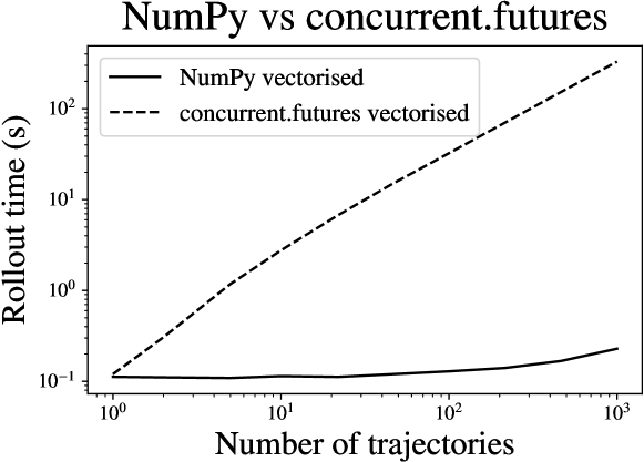
Figure 1. Speedup of vectorization using NumPy.

Name	Arrival process	Mid-price process	Actions	Reward function
Avellaneda and Stoikov (Avellaneda and Stoikov, 2008)	PoissonArrivalModel	BrownianMotionMidpriceModel	limit	ExponentialUtility
Market-making with limit orders (Cartea et al., 2015, Section 10.2)	PoissonArrivalModel	BrownianMotionMidpriceModel	limit	RunningInventoryPenalty
Market-making at the touch (Cartea et al., 2015, Section 10.2.2)	PoissonArrivalModel	BrownianMotionMidpriceModel	touch	RunningInventoryPenalty
Cartea, Jaimungal, and Ricci (CJR) (Cartea et al., 2014)	HawkesArrivalProcess	OuJumpDriftMidpriceModel	limit	RunningInventoryPenalty
Guéant, Lehalle, and Fernandez-Tapia(Guéant et al., 2013) – section 5.2	PoissonArrivalModel	BrownianMotionJumpMidpriceModel	limit	ExponentialUtility
Optimal execution with limit and market orders (Cartea et al., 2015, Section 8.4)	PoissonArrivalModel	BrownianMotionMidpriceModel	limit_and_market	RunningInventoryPenalty

Table 1. Examples of standard models from the literature implemented in mbt_gym

Name	Arrival process	Mid-price process	Actions	Reward function
Avellaneda and Stoikov with Hawkes’ order flows	HawkesArrivalProcess	BrownianMotionMidpriceModel	limit	ExponentialUtility
CJR-14 with pure jump price process	HawkesArrivalProcess	OuJumpDriftMidpriceModel	touch	RunningInventoryPenalty
CJR-14 with exponential utility	HawkesArrivalProcess	OuJumpDriftMidpriceModel	limit	ExponentialUtility

Table 2. Examples of supported hybrid models

3. Baseline agents

We have implemented a number of baseline agents:

• RandomAgent takes a random action in each step.

• FixedActionAgent takes a fixed action in each step.

• FixedSpreadAgent is a market-making agent that maintains a fixed spread (symmetric around the market mid-price).

• HumanAgent allows a human to interact with the environment.

• AvellanedaStoikovAgent is optimal for (Avellaneda and Stoikov, 2008).

• CarteaJaimungalAgent is optimal for (Cartea et al., 2015, Section 10.2).

These agents are useful for learning about models and environments. The AvellanedaStoikovAgent and CarteaJaimungalAgent are useful for benchmarking solutions found by RL; in Section 4, we give an example of training an agent for the CarteaJaimungalAgent setting, and then compare it with the optimal baseline agent.

4. A simple learning example

As an example of training an agent using mbt_gym, we used proximal policy optimization (PPO) (Schulman et al., 2017) to train an agent to solve the market making problem considered in (Cartea et al., 2015, Section 10.2). This problem is a suitable test bed for showing that this approach works since an explicit optimal solution is known. Figure 2 shows the evolution of mean rewards per episode against time for different degrees of vectorization and Figure 3 compares the learnt policy with the optimal policy from (Cartea et al., 2015, Section 10.2).

In Figure 2 it is evident that if the degree of parallelization is too small (n=10 trajectories), then learning is unstable. Similarly, if number of trajectories rolled out in parallel is too large (n=10,000 trajectories), then the (wall-clock) time until convergence starts to increase. There is little difference in the training performance for n=100 and n=1000, but n=1000 outperforms n=100 slightly, with lower variance and convergence to higher mean rewards.

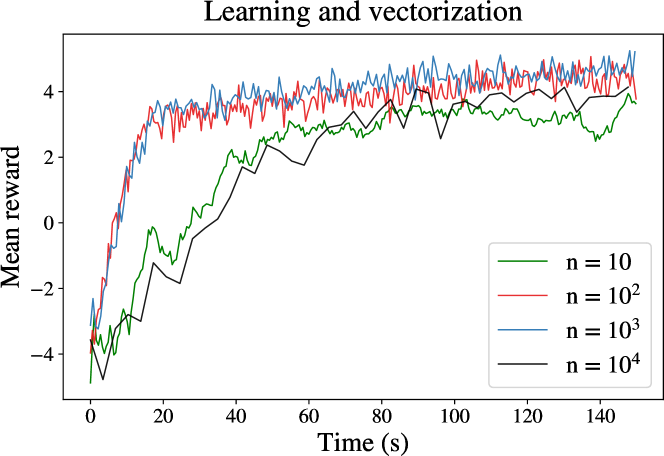
Figure 2. The effect of different degrees of vectorization.

In Figure 3, we see that the agent manages to learn the policy fairly well. The agent learns to skew their bid depth down and their ask depth up when they hold a negative inventory and vice-versa. This induces a mean reversion of the inventory around zero.

In addition to training a PPO agent, we provide an example in the code-base of solving the same problem using vanilla policy gradient, a simpler policy gradient algorithm not in SB3, but implemented by us. To aid learning, the initial inventory can take random integer values in an interval to increase the states that the agent sees.

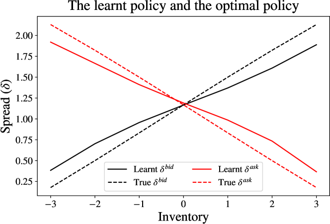
Figure 3. Learnt PPO agent versus CarteaJaimungalAgent.

5. Roadmap for further development

inline,color=purple!40,caption=]Martin: I updated the new reward function names in all tables. I realised that table 3 is never referred to in the text. Do we really need it? (for the workshop paper). If so, we should briefly refer to it. Also I would replace the NAs for Mariariu-Patrichi and Pakkannen by touch and RunningInventoryPenalty.

There are a number of extensions that the gym environment can accommodate in the near future. The examples we give next are categorized into: (i) introducing novel modelling assumptions about the dynamics of the stochastic processes involved, (ii) incorporating the body of literature that deals with optimal execution through trading speeds into the framework, and (iii) presenting mbt_gym working in conjunction with other RL libraries.

Regarding (i), our gym environment is readily suitable for a number of extensions. We can explore the changes in optimal trading strategies once we allow the fill probability model to be influenced by order arrivals, actions, and fills themselves. For example, in an exponential fill probability model, $\mathbb{P}[\text{Fill}]=e^{-\kappa\,\delta}$, where $\delta\geq 0$ is the depth at which the market maker is posted and $\kappa>0$ is the fill exponent, one could take $\kappa$ to be a stochastic process that is affected by arrivals, actions, and fills.

One can also implement the action type touch-and-market, where the agent has control over whether to post at the best quotes, and also when to send a market order for a unit of the asset.

Other extensions can be more challenging to implement, for example, (a) granular arrival of orders given by multi-dimensional Hawkes processes – see Section 5 in (Abergel et al., 2020), or (b) allowing for latency in the framework – see (Gao and Wang, 2020; Cartea and Sánchez-Betancourt, 2021). Let us discuss (b) in a little more detail. In (Cartea and Sánchez-Betancourt, 2021), the time (in the agent’s clock) between an order being sent to the exchange and its execution is exponentially distributed (random latency) or fixed (deterministic latency). Either of these two options can be implemented in our environment by defining the update of the mid-price process in conjunction with a LatencyProcess class (inheriting from StochasticProcess) that defines the (possibly random) delay effects. Then, we update the mid-price process from $t$ to $t+\ell$ where $\ell$ is the latency, perform the transaction at $t+\ell$, and then update the mid-price from $t+\ell$ to $t+\Delta$ where $\Delta$ is the time step – note that we would assume that $\mathbb{P}[\ell\in(0,\Delta]]=1$. By doing so, we track latency effects internally, as opposed to exogenously defining it as an artificial cost.

In terms of (ii), we envisage the implementation of the action type trading_speed, where the control is the trading speed at which the trader is buying or selling. Similar to the fill exponent class, one would need to introduce the price impact class, that will open the door to the study of optimal trading strategies under various price impact functions or processes. Further developments in this direction include the hybrid action types speed-and-limit, or speed-and-touch, where the agent trades at a chosen speed and simultaneously offers liquidity with the hope of getting filled at better prices than those aggressively taken – see (Cartea and Jaimungal, 2015).

For (iii) we would like to integrate RLLib and RLax, as alternatives to Stable Baselines. Finally, a natural extension would be from single-agent RL to multi-agent RL, e.g., to allow the training of RL agents that are robust across model parameters, e.g., as in (Spooner and Savani, 2020).

6. Conclusion

We presented mbt_gym, a library of environments for applying RL to model-based LOB trading problems, along with a development roadmap. We welcome contributions from the wider community.

References

• (1)
• Abergel et al. (2020) Frédéric Abergel, Côme Huré, and Huyên Pham. 2020. Algorithmic trading in a microstructural limit order book model. Quantitative Finance 20, 8 (2020), 1263–1283.
• Almgren (2012) Robert Almgren. 2012. Optimal trading with stochastic liquidity and volatility. SIAM Journal on Financial Mathematics 3, 1 (2012), 163–181.
• Almgren and Chriss (2001) Robert Almgren and Neil Chriss. 2001. Optimal execution of portfolio transactions. Journal of Risk 3 (2001), 5–40.
• Amrouni et al. (2021) Selim Amrouni, Aymeric Moulin, Jared Vann, Svitlana Vyetrenko, Tucker Balch, and Manuela Veloso. 2021. ABIDES-Gym: Gym Environments for Multi-Agent Discrete Event Simulation and Application to Financial Markets. arXiv preprint arXiv:2110.14771 (2021).