An asymptotic study of the joint maximum likelihood estimation of the regularity and the amplitude parameters of a Matérn model on the circle

Abstract

This work considers parameter estimation for Gaussian process interpolation with a periodized version of the Matérn covariance function introduced by Stein. Convergence rates are studied for the joint maximum likelihood estimation of the regularity and the amplitude parameters when the data are sampled according to the model. The mean integrated squared error is also analyzed with fixed and estimated parameters, showing that maximum likelihood estimation yields asymptotically the same error as if the ground truth was known. Finally, the case where the observed function is a fixed deterministic element of a Sobolev space of continuous functions is also considered, suggesting that a joint estimation does not select the regularity parameter as if the amplitude were fixed.

1 Introduction

Gaussian process interpolation or kriging is a common technique for inferring an unknown function from noiseless data, which has applications in geostatistics (Stein, 1999), computer experiments (Santner et al., 2003), and machine learning (Rasmussen and Williams, 2006). A covariance function fully characterizes a zero-mean Gaussian process model. The need for tailoring this function to the task at hand is widely acknowledged in the literature. The common practice consists in choosing it within a parametric family. Stein (1999) promotes using the Matérn (1986) family of stationary covariance functions. Assuming isotropy and using the parameterization from Stein (1999, p. 31), this family is defined on $\mathds{R}^{d}$ by its spectrum:

$$\widehat{k}\colon\omega\in\mathds{R}^{d}\mapsto\frac{\phi}{\left(\alpha^{2}+\lVert\omega\rVert^{2}\right)^{\nu+d/2}},$$ (1)

which is indexed by three parameters: the regularity parameter $\nu$, what we shall call the amplitude parameter $\phi$, and the parameter $\alpha$. See (Stein, 1999) for a comprehensive description of the effect of these parameters. In short, the parameter $\nu$ is shown to be the key quantity governing the asymptotics of the prediction error. The amplitude parameter $\phi$ does not impact the posterior mean predictions but matters for uncertainty quantification, whereas $\alpha$ is less important asymptotically.

One can safely say that cross-validation and maximum likelihood estimation are the most popular techniques for selecting Gaussian process parameters from data. We shall focus on the latter for the rest of this article.

Assuming observations from a Matérn process with parameter $\theta_{0}=\left(\nu_{0},\,\phi_{0},\,\alpha_{0}\right)$, a distinction is often made between increasing and fixed-domain asymptotic frameworks (see, e.g., Bachoc, 2021, for a review). While several increasing-domain asymptotic frameworks have been exhaustively studied (see, e.g., Mardia and Marshall, 1984; Bachoc, 2014), a comprehensive asymptotic analysis of maximum likelihood estimation in fixed-domain frameworks—i.e., on bounded domains—has long been an open question. Previous works mainly consider the estimation of $\phi$ and $\alpha$ for a known $\nu$ (see, e.g., Ying, 1991, 1993; van der Vaart, 1996; Zhang, 2004; Loh, 2006; Kaufman and Shaby, 2013; Li, 2020, who often use alternative parametrizations).

The asymptotics of $\widehat{\nu}_{n}$ seem to have been little studied. Stein (1999, Section 6.7) proposes an asymptotic framework with equispaced observations on the torus and makes a conjecture about the asymptotic behavior of the joint maximum likelihood estimate $\widehat{\theta}_{n}=(\widehat{\nu}_{n},\,\widehat{\phi}_{n},\,\widehat{\alpha}_{n})$ based on the Fisher information matrix (see also Stein, 1993, in the case of noisy observations). This topic has only recently regained popularity. Indeed, Chen et al. (2021) used the framework from Stein to show that $\widehat{\nu}_{n}$ is consistent if the other parameters remain fixed (i.e., enforced to arbitrary values, which may not be $\phi_{0}$ and $\alpha_{0}$). Continuing with fixed $\phi$ and $\alpha$, Karvonen (2023) has recently shown that $\liminf\widehat{\nu}_{n}\geq\nu_{0}$ in the (more general) case of quasi-uniform observations on a “nice” bounded domain of $\mathds{R}^{d}$.

Another long-standing open problem (see notably Putter and Young 2001 and Stein 1999, in the Preface) is that of predictions with estimated parameters: how accurate and reliable are the predictions if one selects a parameter $\widehat{\theta}_{n}$ from data and uses it to make subsequent predictions? The critical influence of $\nu$ on the kriging error suggests that the asymptotic behavior of $\widehat{\nu}_{n}$ is a key element in answering this question.

Another research line consists in studying parameters estimation assuming observations from a fixed deterministic function $f$. The definition of a ground truth $\theta_{0}$ is not obvious in this setting. Instead, the aim is to study which “features” of $f$ are used by the estimator to select a Gaussian process model and how this affects predictions. See (Karvonen et al., 2020; Karvonen and Oates, 2023) for analyses of maximum likelihood estimators of other parameters given a fixed regularity. Regarding $\widehat{\nu}_{n}$, the tight lower bound shown by Karvonen (2023) also covers the case of a continuous function from a Sobolev space. The result shows an interesting connection with sample path properties. More precisely, define the smoothness $\nu_{0}(f)$ of $f$ in a Sobolev sense so that $\nu_{0}(\xi)=\nu_{0}$ holds almost surely for any Matérn process $\xi$ with regularity $\nu_{0}$. For fixed $\phi$ and $\alpha$, Karvonen (2023) showed that $\liminf\widehat{\nu}_{n}\geq\nu_{0}(f)$ and, under (essentially) a self-similarity hypothesis on the spectrum of $f$, that $\widehat{\nu}_{n}$ converges to $\nu_{0}(f)$. This means that, if the spectrum of $f$ is well-behaved, then maximum likelihood estimation fits $\nu$ so that $f$ and the sample paths have the same Sobolev smoothness. It echoes similar findings in Bayesian nonparametric statistics with noise-corrupted observations (see notably Belitser and Ghosal 2003, Knapik et al. 2016, p. 779, and Szabó et al. 2015, pp. 1397 and 1404), where, with our notations, similar conditions on the truth imply that $\widehat{\nu}_{n}\to\nu_{0}(f)$.

This article focuses on the one-dimensional version of the framework proposed by Stein (1999, Section 6.7) to analyze the joint maximum likelihood estimation of $\left(\nu,\phi,\alpha\right)$. This simplified framework is very convenient for such a study, as explained in Section 3. On the one hand, a $\sqrt{n}$-rate asymptotic normality result is shown for $(\widehat{\nu}_{n},\,\widehat{\phi}_{n})$ when observing a Matérn process. Whether the (non-identifiable) parameter $\alpha$ is known or estimated does not affect the limiting distribution. Furthermore, one consequence is that the ratio between the mean squared error with estimated parameters and the one with known parameters converges to unity. On the other hand, it is shown that a joint estimation does not result in the behavior discussed in the previous paragraph. The key takeaway is that only the smaller asymptotic bound $\liminf\widehat{\nu}_{n}\geq\nu_{0}(f)-1/2$ holds. This means that the reproducing kernel Hilbert space is asymptotically too small to contain $f$ but does not say whether the Sobolev smoothness of the sample paths exceeds or converges to $\nu_{0}(f)$. To give a quantitative description of the behavior above $\nu_{0}(f)-1/2$, we derive the large sample limit of the (profile) likelihood on a class of functions that is small but satisfies the usual spectrum conditions ensuring that $\widehat{\nu}_{n}\to\nu_{0}(f)$ for fixed $\phi$ and $\alpha$. The minimizer of this limit has no closed-form expression (see (16)), but we show that a numerical approximation is not maximized by $\nu_{0}(f)$. A strong consistency result on sample paths shows that the set of functions $f$ such that $\widehat{\nu}_{n}\to\nu_{0}(f)$ has probability one under a Matérn process.

To summarize, the contributions of the present article are threefold. First, we prove consistency and asymptotic normality results on the maximum likelihood estimates of the parameters $\nu$ and $\phi$. Then, we leverage these convergence rates to analyze the expected integrated error, showing that estimating the parameters yields the same error asymptotically as if the ground truth was known. Finally, we investigate model selection by maximum likelihood estimation on a deterministic function.

The article is organized as follows. Section 2 introduces the periodic framework and our notations and Section 3 discusses how this framework helps for circumventing the challenges posed by the study of the profile likelihood. Then, Section 4 gives the main results. Finally, Section 5 provides our results on the deterministic case.

2 Gaussian process interpolation on the circle

2.1 Framework

Let $f:\left[0,\,1\right]\to\mathds{R}$ be a continuous periodic function observed on a regular grid: $\{j/n,\ 0\leq j\leq n-1\}$. Consider the periodic version of the Matérn family of stationary covariance functions (1) introduced by Stein (1999, Section 6.7) and defined by the uniformly absolutely convergent Fourier series

$$k_{\theta}\colon x\in\mathds{R}\mapsto\sum_{j\in{\mathds{Z}}}\underline{c}_{j}(\theta)e^{2\pi ixj}$$

with coefficients:

$$\underline{c}_{j}(\theta)=\frac{\phi}{(\alpha^{2}+j^{2})^{\nu+1/2}},\quad\mathrm{for}\,j\in{\mathds{Z}}\ \mathrm{and}\,\theta=(\nu,\phi,\alpha)\in(0,+\infty)^{3}.$$ (2)

The function $k_{\theta}$ is continuous and strictly positive definite (see, e.g., Gneiting, 2011, Theorem 1). The description of the parameters $\nu$, $\phi$, and $\alpha$ from the Introduction carries to this periodic one-dimensional version. A specificity is that $\alpha$ is not identifiable as different values yield equivalent probability measures. However, $\nu$ and $\phi$ are identifiable (see, e.g., Stein, 1999, Chapter 4 and Section 6.7).

Assuming a centered process, the usual task in Gaussian process interpolation is to use the model $\xi\sim\mathrm{GP}\left(0,\,k_{\theta}\right)$ to infer the function $f$ from the noiseless data

$$Z=\left(f\left(0\right),\,f\left(1/n\right),\dots,f\left(1-1/n\right)\right)^{\mathsf{T}}.$$ (3)

The function $f$ is usually predicted using the posterior mean function given by the kriging equations (Matheron, 1971). This predictor can be written simply in the framework presented above.

Proposition 2.1.

Let $n\geq 1$ and $f\colon[0,\,1]\to\mathds{R}$ be a continuous periodic function with absolutely summable Fourier coefficients $c_{j}(f)$. Writing $\widehat{f}_{n}$ for the posterior mean function given $Z$ and the parameter $\theta$, we have:

$$\widehat{f}_{n}(x)=\sum_{j\in{\mathds{Z}}}\left(\frac{\sum_{q\in j+n{\mathds{Z}}}c_{q}(f)}{\sum_{q\in j+n{\mathds{Z}}}\underline{c}_{q}(\theta)}\right)\underline{c}_{j}(\theta)e^{2\pi ixj}\quad\mathrm{for}\ x\in[0,\,1].$$ (4)

The convergence of (4) holds uniformly absolutely.

The proof is deferred to Section A.4 of the Appendix.

The expression (4) shows how the posterior mean function approximates $f$: it transforms the Fourier coefficients of $k_{\theta}$ into those of $f$ using the ratio of their discrete Fourier transforms. Finally, we also define the integrated squared error:

$$\mathrm{ISE}_{n}\left(\nu,\,\alpha;\,f\right)=\int_{0}^{1}\left(f-\widehat{f}_{n}\right)^{2}.$$ (5)

Note that it does not depend on $\phi$.

2.2 Maximum likelihood estimation

Given the observations $Z$ and $\Theta\subset\left(0,\,+\infty\right)^{3}$, a maximum likelihood estimate is defined by $\widehat{\theta}_{n}=(\widehat{\nu}_{n},\widehat{\phi}_{n},\widehat{\alpha}_{n})$ minimizing (a linear transform of) the negative log-likelihood:

$$\mathds{L}_{n}\colon\theta\in\Theta\mapsto n^{-1}\left(\ln\left(\det\left(K_{\theta}\right)\right)+Z^{\mathsf{T}}K_{\theta}^{-1}Z\right),$$ (6)

with ties broken arbitrarily and $K_{\theta}$ the covariance matrix of $Z$ according to $k_{\theta}$.

The estimators $\widehat{\nu}_{n}$ and $\widehat{\alpha}_{n}$ are assumed bounded in this work, i.e., we take $\Theta=N\times\left(0,\,+\infty\right)\times A$ with $N$ and $A$ compact intervals. However, keeping $\widehat{\phi}_{n}$ unbounded is key to our main results and for discussing the deterministic case in Section 5. Write $K_{\theta}=\phi R_{\nu,\alpha}$ for $\theta=\left(\nu,\,\phi,\alpha\right)\in\left(0,\,+\infty\right)^{3}$. The following proposition gives an expression for the profile likelihood, i.e., the infimum of $\mathds{L}_{n}(\nu,\,\phi,\,\alpha)$ with respect to $\phi\in\left(0,\,+\infty\right)$ for fixed $\nu$ and $\alpha$.

Proposition 2.2.

(see, e.g., Santner et al., 2003, Section 3.3.2) Let $\nu,\alpha>0$. It holds that

$$\inf_{\phi>0}\mathds{L}_{n}(\nu,\,\phi,\,\alpha)=1+n^{-1}\ln(\det(R_{\nu,\alpha}))+\ln\left(\frac{Z^{\mathsf{T}}R_{\nu,\alpha}^{-1}Z}{n}\right).$$ (7)

Moreover, if $Z$ is nonzero, then the infimum is uniquely reached by $\widehat{\phi}_{n}=Z^{\mathsf{T}}R_{\nu,\alpha}^{-1}Z/n$.

(The case $Z=0$ is covered since both sides of (7) match.)

3 Studying the profile likelihood using discrete Fourier transforms

3.1 Linking the spectra of $k_{\theta}$ and $K_{\theta}$

As Craven and Wahba (1979) and Stein (1999, Section 6.7) point out, the framework introduced in Section 2.1 is convenient. More precisely, it provides a natural link between $K_{\theta}$ and $k_{\theta}$ using discrete Fourier transforms (see Section A.2 of the Appendix for details). In particular, it gives a closed-form identity

$$n^{-1}\phi\lambda_{m,n}=\sum_{j\in{\mathds{Z}}}\underline{c}_{m+nj}(\theta)$$

linking the eigenvalues $\phi\lambda_{0,n},\dots,\phi\lambda_{n-1,n}$ of $K_{\theta}$ to those of $k_{\theta}$ given by (2). Furthermore, the matrices $K_{\theta}$ share the same eigenvectors. One has $n^{-1}\phi\lambda_{m,n}\to\underline{c}_{m}(\theta)$ for a fixed $m$ but the ratio $n^{-1}\phi\lambda_{m,n}/\underline{c}_{m}(\theta)$ remains bounded away from one for $m$ close to $n/2$.

3.2 The consistency of $\widehat{\nu}_{n}$ for fixed $\phi$ and $\alpha$ (Chen et al., 2021)

Assuming observations from $\xi\sim\mathrm{GP}\left(0,\,k_{\theta_{0}}\right)$ under a similar model with $\theta_{0}=\left(\nu_{0},\,\phi_{0},\,\alpha_{0}\right)\in\left(0,\,+\infty\right)^{3}$, Chen et al. (2021) show the consistency of $\widehat{\nu}_{n}$ for equispaced observations on the $d$-dimensional torus for fixed parameters $\phi$ and $\alpha$. A sketch of their reasoning for $d=1$ is provided in this paragraph. The spectrum of $K_{\theta}$ is studied by showing that

$$n^{-1}\phi\lambda_{m,n}=e^{\mathcal{O}(1)}\underline{c}_{m}(\theta)=e^{\mathcal{O}(1)}m^{-2\nu-1}$$ (8)

uniformly in $\nu$ and $1\leq m\leq n/2$. This approximation yields:

$$\left\{\begin{array}[]{ll}\ln\left(\det\left(K_{\theta}\right)\right)&\,=\,-2\nu n\ln(n)+n\ln(\phi)+n\mathcal{O}(1),\\[5.0pt] Z^{\mathsf{T}}K_{\theta}^{-1}Z&\,=\,\phi^{-1}\phi_{0}\ \mathcal{O}_{\mathsf{P}}\left(\ln(n)\right)\ \mathrm{if}\ \nu\leq\nu_{0}-1/2,\\[5.0pt] Z^{\mathsf{T}}K_{\theta}^{-1}Z&\,=\,\phi^{-1}\phi_{0}\ e^{\mathcal{O}_{\mathsf{P}}(1)}n^{1+2(\nu-\nu_{0})}\ \mathrm{if}\ \nu>\nu_{0}-1/2,\\ \end{array}\right.$$ (9)

with uniform $\mathcal{O}_{\mathsf{P}}$-terms on some regularity ranges. The consistency for fixed parameters $\phi$ and $\alpha$ follows by observing that $\nu_{0}$ is the turning point where the quadratic form starts dominating the log-determinant. The latter claims are also true if $\nu$ is estimated jointly with $\phi\in F$ for a set $F$ bounded away from zero and infinity.

3.3 Profiling the likelihood

Consider now the case $F=\left(0,\,+\infty\right)$ by plugging (9) into (7), for $\nu>\nu_{0}-1/2$, to get

$$\inf_{\phi>0}\mathds{L}_{n}(\nu,\,\phi,\,\alpha)=1+\mathcal{O}(1)+\ln(\phi_{0})+\mathcal{O}_{\mathsf{P}}(1)-2\nu_{0}\ln\left(n\right)=\mathcal{O}_{\mathsf{P}}(1)-2\nu_{0}\ln\left(n\right),$$ (10)

which is not sharp enough. Therefore, a more precise analysis of how the spectrum of $K_{\theta}$ fluctuates around the one of $k_{\theta}$ is needed to study the profile likelihood. The following section provides an ingredient for this purpose. Coordination with tools for proving uniform central limit theorems makes it possible to study convergence rates for parameter estimation and prediction error in Section 4. Developments for studying the profile likelihood are used to provide insights on model selection in the case of a fixed deterministic function from a Sobolev space in Section 5, which also discusses related works in this setting.

3.4 A symmetrized version of the Hurwitz zeta function

Stein (1999, Section 6.7) uses the function

$$\gamma\colon\left(s;\,x\right)\in\left(1,\,+\infty\right)\times\left(0,\,1\right)\mapsto\sum_{j\in{\mathds{Z}}}\frac{1}{\lvert j+x\rvert^{s}},$$

for deriving the asymptotics of the Fisher information matrix of the model presented in Section 2.1. It will also play a major role in our analysis of the likelihood criterion.

The function $\gamma$ is (jointly) smooth and related to the Hurwitz zeta function $\zeta_{H}$ by:

$$\gamma\left(s;\,x\right)=\zeta_{H}(s;\,x)+\zeta_{H}(s;\,1-x),\quad\left(s,\,x\right)\in\left(1,\,+\infty\right)\times\left(0,\,1\right).$$ (11)

Moreover, the function $\gamma\left(s;\cdot\right)$ is symmetric with respect to $1/2$ for $s>1$.

4 Main results

4.1 Standing assumptions

Consider the framework presented in Section 2.1 and suppose that the function is sampled according to the (real-valued) centered Gaussian process:

$$\xi\colon x\in\left[0,\,1\right]\mapsto\frac{1}{\sqrt{2}}\sum_{j\in{\mathds{Z}}}\sqrt{\underline{c}_{j}(\theta_{0})}\left(U_{1,\lvert j\rvert}+iU_{2,\lvert j\rvert}{\mathop{\rm sign}}(j)\right)e^{2\pi ixj},$$ (12)

with $\theta_{0}=(\nu_{0},\phi_{0},\alpha_{0})\in(0,+\infty)^{3}$ and $(U_{q,j})_{q\in\{1,2\},j\geq 0}$ independent random variables such that $U_{2,0}=0$, $U_{1,0}\sim\mathcal{N}\left(0,2\right)$, and $U_{q,j}\sim\mathcal{N}\left(0,1\right)$ for $q\in\{1,2\}$ and $j\geq 1$. Let $\mathsf{P}$ be the measure defined on the underlying probability space (assumed to be the completion of the product space, so the $U_{q,j}$s are coordinate projections). The convergence of the expansion (12) is meant pointwise both in $L^{2}\left(\mathsf{P}\right)$ and almost surely. We further assume $\nu_{0}>1/2$ to avoid dealing with conditionally convergent series. It holds that $\xi\sim\mathrm{GP}\left(0,\,k_{\theta_{0}}\right)$.

Let $\widehat{\theta}_{n}=(\widehat{\nu}_{n},\widehat{\phi}_{n},\widehat{\alpha}_{n})$ be a maximum likelihood estimate as defined in Section 2.2 for some $\Theta=N\times\left(0,\,+\infty\right)\times A$ with $A,N\subset\left(0,\,+\infty\right)$ compact intervals and $\nu_{0}\in N$. The following sections give convergence rates for parameter estimation and prediction error.

4.2 Convergence rates of maximum likelihood estimation

The following result states the strong consistency of $\widehat{\nu}_{n}$.

Theorem 4.1.

Let $\Theta=N\times\left(0,\,+\infty\right)\times A$ with $N$ and $A$ compact intervals and $\nu_{0}\in N$. Then, the convergence $\widehat{\nu}_{n}\to\nu_{0}$ holds almost surely.

The proof is deferred to Section A.5 of the Appendix. A key step is to show that (a shift of) the profile likelihood converges almost surely to

$$\int_{0}^{1}\ln\left(\gamma\left(2\nu+1;\cdot\right)\right)+\ln\left(\int_{0}^{1}\frac{\gamma\left(2\nu_{0}+1;\cdot\right)}{\gamma\left(2\nu+1;\cdot\right)}\right),$$ (13)

for $\nu>\nu_{0}-1/2$. The first term is a refinement of the $\mathcal{O}(1)$ appearing in (9) for the log-determinant. The second term is a refinement of the $\mathcal{O}_{\mathsf{P}}(1)$ appearing for the quadratic form. Jensen inequality shows that (13) is minimized by taking $\nu=\nu_{0}$.

Furthermore, similarly to Stein (1999, Section 6.7), let us define

$$\psi_{\nu}\colon x\in\left(0,\,1\right)\mapsto\frac{\sum_{j\in{\mathds{Z}}}\left|x+j\right|^{-2\nu-1}\ln\left|x+j\right|}{\sum_{j\in{\mathds{Z}}}\left|x+j\right|^{-2\nu-1}},\quad\mathrm{for}\ \nu>0,$$ (14)

which is square integrable on $\left(0,\,1\right)$. The following result proves the conjecture made by Stein (1999, p. 194) when $d=1$ and $\widehat{\nu}_{n}$ and $\widehat{\alpha}_{n}$ are bounded. The proof is deferred to Section A.6 of the Appendix.

Theorem 4.2.

Let $\Theta=N\times\left(0,\,+\infty\right)\times A$ with $N$ and $A$ compact intervals and $\nu_{0}\in N$. Then,

$$\sqrt{2n}\begin{pmatrix}\frac{\widehat{\phi}_{n}-\phi_{0}}{2\phi_{0}}-\left(\ln(n)+\mathsf{E}\left(\psi_{\nu_{0}}(V)\right)\right)\left(\widehat{\nu}_{n}-\nu_{0}\right)\\ \sqrt{\operatorname{Var}\left(\psi_{\nu_{0}}(V)\right)}\left(\widehat{\nu}_{n}-\nu_{0}\right)\\ \end{pmatrix}\leadsto\mathcal{N}\left(0,\,I_{2}\right),$$

where $V$ is a random variable distributed uniformly on $\left(0,\,1\right)$.

Observe that the asymptotic behavior of $(\widehat{\nu}_{n},\,\widehat{\phi}_{n})$ is not influenced by whether the parameter $\alpha$ is fixed, estimated, or even known.

4.3 Convergence rates of the integrated squared error

This section states our results about the expectation of (5) with fixed and estimated parameters. The proofs are deferred to Section C. We begin with the case of fixed parameters.

For $\nu,\nu_{0}>0$, define

$$\vartheta_{\nu;\nu_{0}}\colon x\in\left(0,\,1\right)\mapsto\frac{\gamma\left(4\nu+2;x\right)\gamma\left(2\nu_{0}+1;x\right)}{\gamma^{2}\left(2\nu+1;x\right)}+\gamma\left(2\nu_{0}+1;x\right)-2\frac{\gamma\left(2\nu+2\nu_{0}+2;x\right)}{\gamma\left(2\nu+1;x\right)}$$

which is smooth and integrable when $\nu>(\nu_{0}-1)/2$.

The following result states the asymptotics of the prediction error with fixed parameters.

Theorem 4.3.

Let $\left(\nu,\,\alpha\right)\in\left(0,\,+\infty\right)^{2}$. Then,

$$\mathsf{E}\left(\mathrm{ISE}_{n}\left(\nu,\,\alpha;\,\xi\right)\right)\lesssim\frac{1}{n^{4\nu+2}},\ \mathrm{for}\ \nu<(\nu_{0}-1)/2,$$

$$\mathsf{E}\left(\mathrm{ISE}_{n}\left(\nu,\,\alpha;\,\xi\right)\right)\lesssim\frac{\ln(n)}{n^{2\nu_{0}}},\ \mathrm{for}\ \nu=(\nu_{0}-1)/2,$$

and

$$n^{2\nu_{0}}\mathsf{E}\left(\mathrm{ISE}_{n}\left(\nu,\,\alpha;\,\xi\right)\right)\to\phi_{0}\int_{0}^{1}\vartheta_{\nu;\nu_{0}},\ \mathrm{otherwise}.$$

The symbol $\lesssim$ denotes an inequality up to a universal constant.

This result shows that half of the smoothness is sufficient for optimal convergence rates. However, the constant $\int_{0}^{1}\vartheta_{\nu;\nu_{0}}$ is minimized by taking $\nu=\nu_{0}$. This is in line with the result of Stein (1999, Theorem 3) obtained in a different framework.

Then, our last result gives the asymptotic behavior of the prediction error with estimated parameters.

Theorem 4.4.

Let $\Theta=N\times\left(0,\,+\infty\right)\times A$ with $N$ and $A$ compact intervals and $\nu_{0}\in N$. Then,

$$n^{2\nu_{0}}\mathsf{E}\left(\mathrm{ISE}_{n}\left(\widehat{\nu}_{n},\,\widehat{\alpha}_{n};\,\xi\right)\right)\to\phi_{0}\int_{0}^{1}\vartheta_{\nu_{0};\nu_{0}}.$$

This last result shows that estimating the parameters yields asymptotically the same error as if the ground truth was known.

5 The deterministic case

Let $\beta>1/2$ and define the Sobolev space

$$H^{\beta}\left[0,\,1\right]=\left\{g\in L^{2}\left[0,\,1\right],\ \lVert g\rVert_{H^{\beta}\left[0,\,1\right]}^{2}=\sum_{j\in{\mathds{Z}}}(1+j^{2})^{\beta}\lvert c_{j}(f)\rvert^{2}<+\infty\right\}$$

of (continuous) periodic functions. This section studies maximum likelihood estimation with equispaced observations (3) from a fixed deterministic periodic function $f\colon\left[0,\,1\right]\to\mathds{R}$ lying in a Sobolev space. Define the (Sobolev) smoothness

$$\nu_{0}(f)=\inf\left\{\beta>1/2,\ f\notin H^{\beta}\left[0,\,1\right]\right\}$$

of $f$ as Karvonen (2023) and Wang and Jing (2022). We will assume that $\nu_{0}(f)\in\left(1,\,+\infty\right)$. The restriction $\nu_{0}(f)>1$ is imposed for convenience as it ensures that $f$ has absolutely summable Fourier coefficients. Section D contains the proofs for this section.

On “nice” bounded regions of $\mathds{R}^{d}$, Karvonen (2023) shows that $\liminf\widehat{\nu}_{n}\geq\nu_{0}(f)$ if $\alpha$ and $\phi$ are fixed. Karvonen also shows that $\widehat{\nu}_{n}\to\nu_{0}(f)$ for a class of compactly supported self-similar functions. It is not hard to check that $\nu_{0}(\xi)=\nu$ holds almost surely for any Matérn process with regularity parameter $\nu$. With that in mind, one can interpret the previous results the following way. Maximum likelihood estimation chooses the parameter $\nu$ so that the sample paths are asymptotically smoother than $f$ and, under more assumptions, so that the (Sobolev) smoothnesses match. Interestingly, the proof is close in spirit to the reasoning described in Section 3.2. A sketch is briefly provided with the notations of the framework from Section 2.1. The log-det term in (6) is not data-dependent, so the expansion from (9) applies. Then, for $\nu>\nu_{0}(f)-1/2$, the uniform inequality

$$Z^{\mathsf{T}}K_{\theta}^{-1}Z\lesssim\phi^{-1}n^{1+2(\nu-\nu_{0}(f))}$$

is (essentially) shown. However, establishing (sufficient results slightly weaker than) the reverse inequality requires additional assumptions on $f$, such as membership in a class of functions with self-similar spectra (see Karvonen 2023, Definition 3.1 and also Szabó et al. 2015, p. 1398, in the context of the inverse signal-in-white-noise model). For the present purposes, it suffices to consider the “prototypical” subclass (see Karvonen, 2023, p. 14) of functions $f$ such that

$$C_{1}\left|j\right|^{-\nu_{0}(f)-1/2}\leq\left|c_{j}(f)\right|\leq C_{2}\left|j\right|^{-\nu_{0}(f)-1/2}\quad\mathrm{when}\ \lvert j\rvert\geq N,$$ (15)

for some $N\geq 0$ and $C_{2}\geq C_{1}>0$. This notation is compatible with the definition of $\nu_{0}(f)$. As in previous works, the following property holds for this class of functions with well-behaved spectra.

Proposition 5.1.

Let $\Theta=N\times F\times A$ with $N$, $F$, and $A$ compact intervals and $N$ containing $\nu_{0}(f)$. Assume that $f$ satisfies (15). Then, the convergence $\widehat{\nu}_{n}\to\nu_{0}(f)$ holds.

Having $\phi$ and $\alpha$ estimated on compact intervals jointly with $\nu$ is somewhat anecdotal, so nothing is new in this result. The details of the proof sketched in the previous paragraph are therefore omitted. However, since the proof roughly follows the lines from Section 3.2, the observation from Section 3.3 applies also in this setting. Beforehand, the following preliminary step is required.

Proposition 5.2.

Let $\Theta=N\times\left(0,\,+\infty\right)\times A$ with $N$ and $A$ compact intervals and $\max N\geq\nu_{0}(f)-1/2$. Then, it holds that $\liminf\widehat{\nu}_{n}\geq\nu_{0}(f)-1/2$.

Note the difference with the previous $\liminf\widehat{\nu}_{n}\geq\nu_{0}(f)$ for fixed $\phi$. A smoothness estimate larger than $\nu_{0}(f)$ means that $f$ is rougher than the sample paths. The weaker inequality $\widehat{\nu}_{n}\geq\nu_{0}(f)-1/2$ only means that the function $f$ is rougher than the elements of the reproducing kernel Hilbert space. A computation similar to (10) shows that the behavior above $\nu_{0}(f)-1/2$ is, roughly speaking, governed by $\mathcal{O}(1)$-terms. It is possible to give a quantitative description of what happens for a class smaller than (15). Define

$$\mathds{M}_{n}^{f}\colon\left(\nu,\alpha\right)\in\left(\nu_{0}(f)-1/2,\,+\infty\right)\times\left(0,\,+\infty\right)\mapsto\inf_{\phi>0}\mathds{L}_{n}\left(\nu,\phi,\alpha\right)+2\nu_{0}(f)\ln(n)-1.$$

Proposition 5.3.

Suppose that $c_{j}(f)=\left(1+\mathcal{O}\left(\left|j\right|^{-1}\right)\right)\left|j\right|^{-\nu_{0}(f)-1/2}$ for nonzero $j$. Then, we have

$$\mathds{M}_{n}^{f}\left(\nu,\,\alpha\right)\to\mathds{M}_{\infty}^{f}\left(\nu\right)=\int_{0}^{1}\ln\left(\gamma\left(2\nu+1;\cdot\right)\right)+\ln\left(\int_{0}^{1}\frac{\gamma^{2}\left(\nu_{0}(f)+1/2;\cdot\right)}{\gamma\left(2\nu+1;\cdot\right)}\right),$$ (16)

uniformly on compact subsets of $\left(\nu_{0}(f)-1/2,\,+\infty\right)\times\left(0,\,+\infty\right)$.

We could not identify the minimizer(s) of the limit analytically. Figure 1 shows a numerical approximation to $\mathds{M}_{\infty}^{f}$.

After inspection of the proof of Proposition 5.3, it does not seem obvious to exhibit a function $f$ such that $\widehat{\nu}_{n}\to\nu_{0}(f)$ holds when the amplitude parameter is jointly estimated. However, Theorem 4.1 shows that the set of such functions has probability one under a Matérn process with regularity $\nu_{0}>1/2$ belonging to $N$.

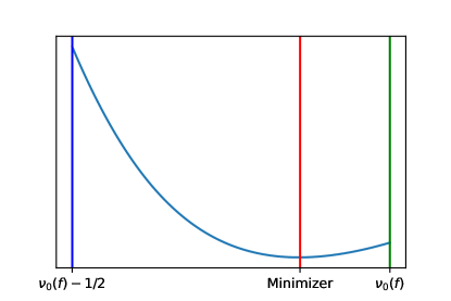
Figure 1: The function $\mathds{M}_{\infty}^{f}$, for $\nu_{0}(f)=3/2$. A numerical approximation to the minimizer is about $1.359$. Note that $\mathds{M}_{\infty}^{f}$ is approximated numerically using finite sums for $\gamma$ and discretizations for the integrals.

Acknowledgments.

The author thanks Julien Bect and Emmanuel Vazquez for their patience and guidance.

Appendix A Proofs

A.1 Notations

The symbol $\lesssim$ denotes an inequality up to a universal constant. For compactness, the symbol $\approx$ is used when the two-way inequality $\lesssim$ holds.

Write $K_{\theta}=\phi R_{\nu,\alpha}$ and $\underline{c}_{j}(\theta)=\phi c_{j}(\nu,\alpha)$, for $\theta=\left(\nu,\,\phi,\alpha\right)\in\left(0,\,+\infty\right)^{3}$ and $j\in{\mathds{Z}}$. All results suppose that $\Theta=N\times\left(0,\,+\infty\right)\times A$ with $N=\left[\nu_{\min},\,\nu_{\max}\right]$, $A=\left[\alpha_{\min},\,\alpha_{\max}\right]$, $0<\nu_{\min}<\nu_{0}<\nu_{\max}<+\infty$, and $0<\alpha_{\min}\leq\alpha_{\max}<+\infty$ unless explicitly stated otherwise. Without loss of generality, suppose that $\nu_{\min}<\nu_{0}-1/2$ and define $N_{\epsilon}=\left[\nu_{0}-1/2+\epsilon,\,+\infty\right)\cap N$ for $\epsilon>0$. The notation $l=\left\lfloor(n-1)/2\right\rfloor$ will often be used throughout the following.

A.2 Circulant matrices and useful facts

The framework introduced in Section 2.1 is convenient for analyzing kernel-based regression methods (see, e.g., Craven and Wahba, 1979). This section reviews the properties needed for our purposes.

Let $W$ be the $n\times n$ matrix with entries $W_{j,m}=n^{-1/2}e^{2\pi ijm/n}$, for $0\leq j,m\leq n-1$. For every $\theta=(\nu,\phi,\alpha)\in(0,+\infty)^{3}$, the periodicity of $k_{\theta}$ implies that

$$K_{\theta}=\begin{pmatrix}k_{\theta}\left(0\right)\,&k_{\theta}\left(\frac{1}{n}\right)\,&\dots\,&k_{\theta}\left(\frac{n-1}{n}\right)\\[6.0pt] k_{\theta}\left(\frac{n-1}{n}\right)&\,k_{\theta}\left(0\right)&\,\dots&\,k_{\theta}\left(\frac{n-2}{n}\right)\\[6.0pt] \dots&\,\dots&\,\dots&\,\dots\\[6.0pt] k_{\theta}\left(\frac{1}{n}\right)&\,k_{\theta}\left(\frac{2}{n}\right)&\,\dots&k_{\theta}\left(0\right)\end{pmatrix}$$

is a circulant matrix and so is $R_{\nu,\alpha}$. Consequently (see, e.g., Brockwell and Davis, 1987, p. 130), it holds that $R_{\nu,\alpha}=W\Delta_{\nu,\alpha}W^{\ast}$ with $\Delta_{\nu,\alpha}=\mathrm{diag}\left(\lambda_{0,n},\dots,\lambda_{n-1,n}\right)$ and

$$\lambda_{m,n}=\sum_{j=0}^{n-1}e^{-2\pi ijm/n}k_{\nu,1,\alpha}(j/n)=n\sum_{j\in{\mathds{Z}}}c_{m+nj}(\nu,\,\alpha),\ 0\leq m\leq n-1.$$ (17)

Note that $\lambda_{m,n}$ depends on $\nu$ and $\alpha$ but the symbols are dropped to avoid cumbersome expressions. These coefficients verify

$$\lambda_{m,n}=\lambda_{n-m,n},\ \mathrm{for}\ 1\leq m\leq n-1.$$ (18)

The eigenvalue $\lambda_{0,n}$ is simple and there are $l$ pairs $\left(\lambda_{m,n},\,\lambda_{n-m,n}\right)$, for $m\in\llbracket 1,\,l\rrbracket$, where $l$ is the shortcut defined in Section A.1. If $n$ is even, then the eigenvalue $\lambda_{n/2,n}$ is also simple.

Furthermore, combining each pair of eigenvectors of $W$ shows that $R_{\nu,\alpha}=P\Delta_{\nu,\alpha}P^{\mathsf{T}}$ for a unitary matrix $P$ written using sines and cosines functions. Then, with $\theta_{0}=\left(\nu_{0},\phi_{0},\alpha_{0}\right)$ the ground truth introduced in Section 4.1, write

$$P^{\mathsf{T}}Z=\sqrt{\phi_{0}}\left(\sqrt{\lambda_{0,n}^{(0)}}U_{0,n},\dots,\sqrt{\lambda_{n-1,n}^{(0)}}U_{n-1,n}\right),$$

with $\lambda_{0,n}^{(0)},\dots,\lambda_{n-1,n}^{(0)}$ the eigenvalues of $R_{\nu_{0},\alpha_{0}}$ and $U_{0,n},\dots,U_{n-1,n}$ drawn independently from a standard Gaussian. We have

$$Z^{\mathsf{T}}R_{\nu,\alpha}^{-1}Z=\phi_{0}\sum_{m=0}^{n-1}\frac{U_{m,n}^{2}\lambda_{m,n}^{(0)}}{\lambda_{m,n}}.$$

Our strategy to analyze this kind of expression will often consist of: 1) studying the sum for $m\in\llbracket 1,\,l\rrbracket$; 2) using the equality (18); and 3) treating the remaining terms for $m=0$ and eventually $m=n/2$ separately.

The following approximation discussed in Section 3.2 will sometimes be used.

Lemma A.1.

One has $n^{-1}\lambda_{0,n}\approx c_{0}(\nu,\alpha)\approx 1$ and $n^{-1}\lambda_{m,n}\approx c_{m}(\nu,\alpha)\approx m^{-2\nu-1}$ uniformly in $\nu\in N$, $\alpha\in A$, $n$ and $1\leq m\leq\left\lfloor n/2\right\rfloor$.

Proof.

Let $0\leq m\leq\left\lfloor n/2\right\rfloor$, we have using (17)

$$c_{m}(\nu,\alpha)\leq\lambda_{m,n}/n\leq 2c_{m}(\nu,\alpha)+2\sum_{j=1}^{+\infty}c_{m+nj}(\nu,\alpha).$$

Moreover

$$\sum_{j=1}^{+\infty}c_{m+nj}(\nu,\alpha)/c_{m}(\nu,\alpha)\leq\sum_{j=1}^{+\infty}(\alpha_{\max}^{2}+1/4)^{\nu+1/2}/j^{2\nu+1}\lesssim 1,$$

uniformly using the monotonicity of the zeta function. This shows $n^{-1}\lambda_{m,n}\approx c_{m}(\nu,\alpha)$ and finishing the proof makes no difficulty. ∎

Nevertheless, our results will require refined approximations, as explained in Section 3.3.

A.3 More notations and properties

For each $n$, it is straightforward to prove that the $\lambda_{m,n}$s are smooth functions of $\left(\nu,\,\alpha\right)\in\left(0,\,+\infty\right)^{2}$ by bounding the derivatives of the $c_{j}$s uniformly on compacta (up to third-order derivatives suffice for our purposes). Using the formulas from Section A.2 then shows that $\mathds{L}_{n}$ is also smooth for any realization.

Furthermore, define:

$$\mathds{M}_{n}\colon\left(\nu,\alpha\right)\in N\times A\mapsto\inf_{\phi>0}\mathds{L}_{n}\left(\nu,\phi,\alpha\right)+2\nu_{0}\ln(n)-\ln\left(\phi_{0}\right)-1,$$

with $\nu_{0}$ the ground truth introduced in Section 4.1. Its expression is given by Proposition 2.2 so it is a stochastic process which is smooth on the almost sure event $Z\neq 0$. The proofs mostly consist in studying $\mathds{M}_{n}$.

For a compact interval $A\subset\left(0,\,+\infty\right)$, define now $\mathds{U}_{n}\colon\nu\in N\mapsto\inf_{\alpha\in A}\mathds{M}_{n}\left(\nu,\alpha\right)$. The object $\mathds{U}_{n}$ is a stochastic process since the infima can be replaced by countable ones. Its almost sure continuity follows from the almost sure smoothness of $\mathds{M}_{n}$ and the compacity of $A$.

Also, write $g_{\nu}=\ln\left(\gamma\left(2\nu+1;\,\cdot\right)\right)$ for $\nu>0$ and

$$h_{\nu;\nu_{0}}=\frac{\gamma\left(2\nu_{0}+1;\,\cdot\right)}{\gamma\left(2\nu+1;\,\cdot\right)}$$

for $\nu>\nu_{0}-1/2$. These functions are smooth and integrable and we will write

$$H\colon\nu\in\left(\nu_{0}-1/2,\,+\infty\right)\mapsto\int_{0}^{1}h_{\nu;\nu_{0}},\quad G\colon\nu\in\left(0,\,+\infty\right)\mapsto\int_{0}^{1}g_{\nu},$$

and $\mathds{U}\colon\nu\in\left(\nu_{0}-1/2,\,+\infty\right)\mapsto G(\nu)+\ln\left(H(\nu)\right)$. The smoothness of these functions is ensured by dominated convergence arguments (three derivatives suffice for our purposes).

A.4 Proofs of Section 2.1

Proof of Proposition 2.1.

For $x\in\left[0,\,1\right]$, the kriging equations yield $\widehat{f}_{n}(x)=k_{\theta,\,x}^{\mathsf{T}}\,K_{\theta}^{-1}Z$, with $k_{\theta,\,x}=\left(k_{\theta}\left(m/n-x\right)\right)_{0\leq m\leq n-1}$. The assumptions guarantee that $f$ equals the limit of its Fourier series everywhere. Then, using the matrix $W$ defined in Section A.2, it is straightforward to show that

$$W^{\ast}Z=\sqrt{n}\left(\sum_{j\in m+n{\mathds{Z}}}c_{j}(f)\right)_{0\leq m\leq n-1}$$ (19)

and

$$W^{\ast}k_{\theta,\,x}=\sqrt{n}\left(\sum_{j\in m+n{\mathds{Z}}}\underline{c}_{j}(\theta)e^{-2\pi ixj}\right)_{0\leq m\leq n-1},$$

where the sums converge absolutely. Then, the uniform absolute-convergence of (4) follows from elementary manipulations. ∎

A.5 Proof of Theorem 4.1

A.5.1 Proof of the theorem

Proof of Theorem 4.1.

For $0<\epsilon<1/2$, the sequence $\mathds{U}_{n}$ converges almost surely uniformly to $\mathds{U}$ on $N_{\epsilon}$ by Lemma A.6. Also, the function $\mathds{U}$ is continuous and strictly minimized by taking $\nu=\nu_{0}$ thanks to Jensen inequality.

The rest of the proof is dedicated to showing that $\liminf\widehat{\nu}_{n}\geq\nu_{0}-1/2+\epsilon$ for some $\epsilon>0$. First for $\nu\in N$ and $\alpha\in A$, we have

$$\mathds{M}_{n}(\nu,\alpha) \,=\,G(\nu)+\mathcal{O}\left(\ln(n)/n\right)+\ln\left(\frac{\phi_{0}^{-1}Z^{\mathsf{T}}R_{\nu,\alpha}^{-1}Z}{n^{1+2(\nu-\nu_{0})}}\right)$$

$$\,=\,\mathcal{O}\left(1\right)+\ln\left(\frac{\phi_{0}^{-1}Z^{\mathsf{T}}R_{\nu,\alpha}^{-1}Z}{n^{1+2(\nu-\nu_{0})}}\right)$$

uniformly in $\nu\in N$ and $\alpha\in A$ thanks to Lemma A.5 and the continuity of $G$.

Now, let $0<\epsilon<1/4$, $\nu\in N\setminus N_{\epsilon}=\left[\nu_{\min},\,\nu_{0}-1/2+\epsilon\right)$ and $\alpha\in A$. It holds that:

$$\frac{\phi_{0}^{-1}Z^{\mathsf{T}}R_{\nu,\alpha}^{-1}Z}{n^{1+2(\nu-\nu_{0})}} \,\geq\,\frac{C}{n}\sum_{m=1}^{n-1}U_{m,n}^{2}\min\left(\frac{m}{n},1-\frac{m}{n}\right)^{2(\nu-\nu_{0})}\quad\left(C>0,\ \mathrm{by\ Lemma\leavevmode\nobreak\ }\ref{lem:rough_bound_c}\ \mathrm{and}\ \eqref{eq:eigen_sym}\right)$$

$$\,\geq\,\frac{C}{n}\sum_{m=1}^{n-1}U_{m,n}^{2}\min\left(\frac{m}{n},1-\frac{m}{n}\right)^{-1+2\epsilon}\quad\left(\nu\leq\nu_{0}-1/2+\epsilon\right)$$

$$\,=\,o(1)+\frac{C}{n}\sum_{m=1}^{n-1}\min\left(\frac{m}{n},1-\frac{m}{n}\right)^{-1+2\epsilon}\quad\left(\mathrm{a.s.,\ using\ Lemma\leavevmode\nobreak\ }\ref{lem:riemann_sum_bound}\right)$$

$$\,\to\,\frac{C}{2^{2\epsilon}\epsilon}.$$

Lemma A.6 gives $\mathds{U}_{n}\left(\nu_{0}\right)\to\mathds{U}\left(\nu_{0}\right)$ almost surely, so we have

$$\inf_{\nu\in N\setminus N_{\epsilon}}\mathds{U}_{n}\left(\nu\right)-\mathds{U}_{n}\left(\nu_{0}\right) \,=\,\inf_{\nu\in N\setminus N_{\epsilon},\alpha\in A}\mathds{M}_{n}(\nu,\alpha)-\mathds{U}_{n}\left(\nu_{0}\right)$$

$$\,\geq\,\mathcal{O}(1)+\ln\left(C\right)-\ln\left(2^{2\epsilon}\epsilon\right)-\mathds{U}\left(\nu_{0}\right)+o\left(1\right).$$

Letting $\epsilon\to 0$ shows that the expression in display can be made almost surely ultimately strictly positive. ∎

A.5.2 Approximating $\ln(\det(R_{\nu,\alpha}))$

Lemma A.2.

Let $\nu\in N$, $\alpha\in A$, $1\leq m\leq\left\lfloor n/2\right\rfloor$, and $j\in{\mathds{Z}}$. We have:

$$c_{m+nj}(\nu,\alpha)=\frac{1+u_{n,m,j}(\nu,\alpha)}{\lvert jn+m\rvert^{2\nu+1}},$$ (20)

with $-1<v_{m}\leq u_{n,m,j}(\nu,\alpha)\leq 0$ and $v_{m}=\mathcal{O}(m^{-2})$.

Proof.

Using (17), we have

$$c_{m+nj}(\nu,\alpha)=\frac{1}{(\alpha^{2}+(jn+m)^{2})^{\nu+1/2}}=\frac{1+u_{n,m,j}(\nu,\alpha)}{\lvert jn+m\rvert^{2\nu+1}},$$

with $u_{n,m,j}(\nu,\alpha)=\left(1+(\alpha/(jn+m))^{2}\right)^{-\nu-1/2}-1$. Elementary operations show that

$$0\geq u_{n,m,j}(\nu,\alpha)\geq\left(\left(\frac{\alpha_{\max}}{m}\right)^{2}+1\right)^{-\nu_{\max}-1/2}-1,$$

which gives the desired result thanks to the Taylor inequality. ∎

Lemma A.3.

Let $S\subset\left(1,\,+\infty\right)$ be a compact interval. It holds that

$$\gamma\left(s;\,x\right)=\frac{1}{x^{s}}+\frac{1}{(1-x)^{s}}+\mathcal{O}\left(1\right),$$

uniformly in $s\in S$ and $x\in\left(0,\,1\right)$. In particular, we have $\gamma\left(s;\,x\right)\approx\min\left(x,\,1-x\right)^{-s}$.

Proof.

Let $s_{\min}=\min S$. Then, $0\leq\gamma\left(s;\,x\right)-x^{-s}-(1-x)^{-s}\leq 2\zeta(s_{\min})$. ∎

Lemma A.4.

Let $S\subset\left(1,\,+\infty\right)$ be a compact interval. It holds that

$$\frac{\partial\gamma}{\partial s}\left(s;\,x\right)=-\frac{\ln(x)}{x^{s}}-\frac{\ln(1-x)}{(1-x)^{s}}+\mathcal{O}\left(1\right),$$

uniformly in $s\in S$ and $x\in\left(0,\,1\right)$.

Proof.

Similar to the proof of Lemma A.3. ∎

Lemma A.5.

Uniformly in $\nu\in N$ and $\alpha\in A$, we have

$$\ln(\det(R_{\nu,\alpha}))=-2\nu n\ln(n)+n\int_{0}^{1}g_{\nu}+\mathcal{O}(\ln(n)).$$

Proof.

Let $\nu\in N$ and $\alpha\in A$. Using (17) and Lemma A.2, we have

$$\lambda_{m,n}/n=\sum_{j\in{\mathds{Z}}}c_{m+nj}(\nu,\alpha)=\sum_{j\in{\mathds{Z}}}\frac{1+u_{n,m,j}(\nu,\alpha)}{\lvert jn+m\rvert^{2\nu+1}}.$$

Therefore, using the notation $l=\left\lfloor(n-1)/2\right\rfloor$, we have

$$\sum_{m=1}^{l}\ln(\lambda_{m,n}/n)=-(2\nu+1)l\ln(n)+a_{n}\left(\nu,\,\alpha\right)+\sum_{m=1}^{l}g_{\nu}(m/n),$$

with

$$\left|a_{n}\left(\nu,\,\alpha\right)\right|\leq\left|\sum_{m=1}^{l}\ln(1+v_{m})\right|=\mathcal{O}(1)$$

uniformly in $\nu\in N$ and $\alpha\in A$.

The function $g_{\nu}$ is symmetric with respect to $1/2$. Moreover, a direct consequence of Lemma A.3 is that

$$g_{\nu}(x)=-(2\nu+1)\ln(x)+\mathcal{O}\left(1\right),$$ (21)

uniformly in $\nu\in N$ and $0<x\leq 1/2$. For $\nu\in N$, the function $g_{\nu}$ is thus integrable on $\left(0,\,1\right)$. Furthermore, verifying that it is non-increasing on $\left(0,\,1/2\right]$ is straightforward using the derivative of $\gamma\left(2\nu+1;\,\cdot\right)$, so we have:

$$\int_{1/n}^{(l+1)/n}g_{\nu}\leq\frac{1}{n}\sum_{m=1}^{l}g_{\nu}(m/n)\leq\int_{0}^{l/n}g_{\nu}.$$

Use then (21) to get $\int_{0}^{1/n}g_{\nu}=\mathcal{O}(\ln(n)/n)$, uniformly in $\nu\in N$. The remainders $\int_{l/n}^{1/2}g_{\nu}$ and $\int_{1/2}^{(l+1)/n}g_{\nu}$ are $\mathcal{O}(n^{-1})$ uniformly in $\nu\in N$ by a compacity argument using the continuity of $\gamma$.

Therefore, we have

$$\sum_{m=1}^{l}g_{\nu}(m/n)=n\int_{0}^{1/2}g_{\nu}+\mathcal{O}(\ln(n)),$$

uniformly in $\nu\in N$. Moreover, Lemma A.1 shows that $\ln\left(\lambda_{0,n}/n\right)=\mathcal{O}(1)$ and $\ln\left(\lambda_{n/2,n}/n\right)=\mathcal{O}(\ln(n))$ uniformly for $n$ even. One can then conclude using (18). ∎

A.5.3 Approximating $Z^{\mathsf{T}}R_{\nu,\alpha}Z$

Let us first give some definitions. For $\epsilon>0$, Lemma A.3 can be used to show that there exists some $C>0$ such that

$$h_{\nu;\nu_{0}}(x)\leq F_{\epsilon}(x)=C\min(x,1-x)^{-1+2\epsilon},\ \mathrm{for\ all}\ 0<x<1\ \mathrm{and}\ \nu\in N_{\epsilon}.$$ (22)

The function $F_{\epsilon}$ will be called the envelope of the family $\mathcal{F}_{\epsilon}=\{h_{\nu;\nu_{0}},\ \nu\in N_{\epsilon}\}$ of functions.

Lemma A.6.

For $0<\epsilon<1/2$, the sequence $\mathds{M}_{n}$ converges almost surely uniformly to $\left(\nu,\,\alpha\right)\mapsto\mathds{U}\left(\nu\right)$ on $N_{\epsilon}\times A$.

Proof.

For $\nu\in N_{\epsilon}$ and $\alpha\in A$, we have:

$$\frac{\phi_{0}^{-1}Z^{\mathsf{T}}R_{\nu,\alpha}^{-1}Z}{n^{1+2(\nu-\nu_{0})}}-\int_{0}^{1}h_{\nu;\nu_{0}}$$ (23)

$$=\frac{U_{0,n}^{2}\lambda_{0,n}^{(0)}}{n^{1+2(\nu-\nu_{0})}\lambda_{0,n}}+\frac{1}{n}\sum_{m=1}^{n-1}U_{m,n}^{2}\left(\frac{\lambda_{m,n}^{(0)}}{n^{2(\nu-\nu_{0})}\lambda_{m,n}}-h_{\nu;\nu_{0}}\left(m/n\right)\right)$$

$$+\frac{1}{n}\sum_{m=1}^{n-1}B_{m,n}h_{\nu;\nu_{0}}\left(m/n\right)+\left(\frac{1}{n}\sum_{m=1}^{n-1}h_{\nu;\nu_{0}}\left(m/n\right)-\int_{0}^{1}h_{\nu;\nu_{0}}\right),$$

with $B_{m,n}=U_{m,n}^{2}-1$. First, $\sup_{\nu\in N_{\epsilon}}\left|n^{-1}\sum_{m=1}^{n-1}B_{m,n}h_{\nu;\nu_{0}}\left(m/n\right)\right|$ converges almost surely to zero by Lemma A.11, Lemma A.13, and Arzelà-Ascoli theorem. Then, for all $\beta>0$, a Borel-Cantelli argument shows that $U_{0,n}^{2}\lesssim n^{\beta}$ almost surely, so the $m=0$-term converges almost surely uniformly to zero by Lemma A.1. Finally, Lemma A.8 and Lemma A.10 show that (23) converges almost surely uniformly. Conclude using Proposition 2.2, Lemma A.5, and the $L^{\infty}$-continuity at $H\colon\left(\nu,\,\alpha\right)\in N_{\epsilon}\times A\mapsto\int_{0}^{1}h_{\nu;\nu_{0}}$ of the mapping $\psi$ used in the proof of Lemma A.16. ∎

Lemma A.7.

The function $h_{\nu;\nu_{0}}$ is non-decreasing (resp. non-increasing) on $(0,1/2]$ when $\nu\geq\nu_{0}$ (resp. $\nu\leq\nu_{0}$).

Proof.

Suppose that $\nu\geq\nu_{0}$. Use (11) along with the fact that the Hurwitz Zeta function verifies

$$\frac{\partial\zeta_{H}}{\partial x}(s;\ x)=-s\zeta_{H}(s+1;\ x),\quad\mathrm{for}\ x>0,\ \mathrm{and}\ s>1,$$ (24)

and has the representation

$$\zeta_{H}(s;\ x)=\frac{1}{\Gamma(s)}\int_{0}^{+\infty}\frac{t^{s-1}e^{-tx}}{1-e^{-t}}\mathrm{d}t,\quad\mathrm{for}\ x>0,\ \mathrm{and}\ s>1,$$

where $\Gamma$ is the classical Gamma function (see, e.g., Postnikov, 1988). So, for $x\in\left(0,\,1\right)$, we have

$$\gamma\left(2\nu+1;\,x\right)=\frac{1}{\Gamma(2\nu+1)}\int_{0}^{+\infty}\frac{t^{2\nu}(e^{-tx}+e^{-t(1-x)})}{1-e^{-t}}\mathrm{d}t,$$

and

$$\frac{\partial\gamma}{\partial x}\left(2\nu+1;\,x\right)=\frac{1}{\Gamma(2\nu+1)}\int_{0}^{+\infty}\frac{t^{2\nu+1}(e^{-t(1-x)}-e^{-tx})}{1-e^{-t}}\mathrm{d}t.$$

Now let $x\in[1/2,1)$, the derivative of $h_{\nu;\nu_{0}}$ at $x$ has the sign of

$$\gamma\left(2\nu+1;\,x\right)\frac{\partial\gamma}{\partial x}\left(2\nu_{0}+1;\,x\right)-\gamma\left(2\nu_{0}+1;\,x\right)\frac{\partial\gamma}{\partial x}\left(2\nu+1;\,x\right)$$

$$=\frac{1}{\Gamma(2\nu+1)\Gamma(2\nu_{0}+1)}\int_{0}^{+\infty}\int_{0}^{+\infty}\frac{t^{2\nu}s^{2\nu_{0}}(\eta(s,t;x)-\eta(t,s;x))}{\kappa(s,t)}\mathrm{d}t\mathrm{d}s$$

with $\eta(s,t;x)=s(e^{-tx}+e^{-t(1-x)})(e^{-s(1-x)}-e^{-sx})$ and $\kappa(s,t)=(1-e^{-t})(1-e^{-s})=\kappa(t,s)$ thanks to the Fubini-Lebesgue theorem. Then, one can split the integral to have:

$$\frac{1}{\Gamma(2\nu+1)\Gamma(2\nu_{0}+1)}\left(\int_{0}^{+\infty}\int_{t}^{+\infty}\frac{t^{2\nu}s^{2\nu_{0}}(\eta(s,t;x)-\eta(t,s;x))}{\kappa(s,t)}\mathrm{d}t\mathrm{d}s\right.$$

$$\left.+\int_{0}^{+\infty}\int_{t}^{+\infty}\frac{s^{2\nu}t^{2\nu_{0}}(\eta(t,s;x)-\eta(s,t;x))}{\kappa(t,s)}\mathrm{d}t\mathrm{d}s\right)$$

$$=\frac{1}{\Gamma(2\nu+1)\Gamma(2\nu_{0}+1)}\int_{0}^{+\infty}\int_{t}^{+\infty}\frac{(t^{2\nu}s^{2\nu_{0}}-s^{2\nu}t^{2\nu_{0}})(\eta(s,t;x)-\eta(t,s;x))}{\kappa(s,t)}\mathrm{d}t\mathrm{d}s\leq 0$$

since $t^{2\nu}s^{2\nu_{0}}\leq s^{2\nu}t^{2\nu_{0}}$ when $s\geq t$, $\kappa(s,t)\geq 0$ and $\eta(s,t;x)\geq\eta(t,s;x)$ when $s\geq t$ and $x\geq 1/2$.

So we proved that $h_{\nu;\nu_{0}}$ is non-increasing on $[1/2,1)$ and the first claim is due to the symmetry with respect to $1/2$. Observe that $h_{\nu;\nu_{0}}=1/h_{\nu_{0};\nu}$ for the second claim. ∎

Lemma A.8.

Let $\epsilon>0$, we have

$$\frac{1}{n}\sum_{m=1}^{n-1}h_{\nu;\nu_{0}}(m/n)=\int_{0}^{1}h_{\nu;\nu_{0}}+\mathcal{O}\left(\frac{1}{n^{\min(1,\ 2\epsilon)}}\right),$$

uniformly in $\nu\in N_{\epsilon}$.

Proof.

The proof is similar to the treatment of $n^{-1}\sum_{m=1}^{n-1}g_{\nu}(m/n)$ in the proof of Lemma A.5 using Lemma A.7 and (22) to get:

$$\int_{0}^{1/n}h_{\nu;\nu_{0}}\leq\int_{0}^{1/n}F_{\epsilon}=\mathcal{O}(n^{-2\epsilon}),\quad\mathrm{uniformly\ in}\ \nu\in N_{\epsilon}.$$ (25)

∎

Lemma A.9.

Let $1\leq m\leq\left\lfloor n/2\right\rfloor$, we have

$$\frac{\lambda_{m,n}^{(0)}}{n^{2(\nu-\nu_{0})}\lambda_{m,n}}=\left(1+\mathcal{O}(m^{-2})\right)h_{\nu;\nu_{0}}(m/n)$$

uniformly in $\nu\in N$ and $\alpha\in A$.

Proof.

A direct consequence from Lemma A.2. ∎

Lemma A.10.

Let $0<\epsilon<1/2$ and $0<\delta<2\epsilon$. There exists a constant $C$ such that

$$\limsup n^{2\epsilon-\delta}\sup_{(\nu,\alpha)\in N_{\epsilon}\times A}\frac{1}{n}\sum_{m=1}^{n-1}U_{m,n}^{2}\left|\frac{\lambda_{m,n}^{(0)}}{n^{2(\nu-\nu_{0})}\lambda_{m,n}}-h_{\nu;\nu_{0}}\left(\frac{m}{n}\right)\right|\leq C,$$

almost surely.

Proof.

Let $\nu\in N_{\epsilon}$, $\alpha\in A$, and $p=1/(1-2\epsilon+\delta)$. It holds that $n^{-1}\sum_{m=1}^{n-1}F_{\epsilon}^{p}(m/n)=\mathcal{O}(1)$. Then, Lemma A.9, the usual symmetry arguments, and Hölder inequality yield:

$$\frac{1}{n}\sum_{m=1}^{n-1}U_{m,n}^{2}\left|\frac{\lambda_{m,n}^{(0)}}{n^{2(\nu-\nu_{0})}\lambda_{m,n}}-h_{\nu;\nu_{0}}\left(\frac{m}{n}\right)\right|$$

$$\,=\,\frac{1}{n}\sum_{m=1}^{n-1}U_{m,n}^{2}\mathcal{O}\left(m^{-2}\vee(n-m)^{-2}\right)h_{\nu;\nu_{0}}\left(\frac{m}{n}\right)$$

$$\,\leq\,\frac{1}{n^{1/q}}\cdot\left(\frac{1}{n}\sum_{m=1}^{n-1}\left|U_{m,n}\right|^{2p}F_{\epsilon}^{p}(m/n)\right)^{1/p}\cdot\underbrace{\left(\sum_{m=1}^{n-1}\mathcal{O}\left(m^{-2q}\vee(n-m)^{-2q}\right)\right)^{1/q}}_{\mathcal{O}(1)\ \mathrm{uniformly}}$$

with $1/q=2\epsilon-\delta$. Conclude using Lemma A.12 and $n^{-1}\sum_{m=1}^{n-1}F_{\epsilon}^{p}(m/n)=\mathcal{O}(1)$. ∎

For $n\geq 2$ and $1\leq m\leq n-1$, define $B_{m,n}=U_{m,n}^{2}-1$.

Lemma A.11.

Let $\nu>\nu_{0}-1/2$. Then, $n^{-1}\sum_{m=1}^{n-1}B_{m,n}h_{\nu;\nu_{0}}\left(m/n\right)$ converges almost surely to zero.

Proof.

A direct consequence of Lemma A.12, since $0\leq h_{\nu;\nu_{0}}(x)\lesssim\min\left(x,\,1-x\right)^{2(\nu-\nu_{0})}$. ∎

Lemma A.12.

Let $\alpha>-1$ and $g\colon\left(0,\,1\right)\to\mathds{R}$ such that $0\leq g(x)\lesssim\min\left(x,\,1-x\right)^{\alpha}$. For each $n$, let $D_{1,n},\dots,D_{n-1,n}$ be i.i.d. centered variables such that $\mathsf{E}(\left|D_{1,2}\right|^{q})$ is finite for all $q\geq 0$. Then, $n^{-1}\sum_{m=1}^{n-1}D_{m,n}g\left(m/n\right)$ converges almost surely to zero.

Proof.

If $\alpha\geq 0$, then $g\left(m/n\right)=\mathcal{O}(1)$, so the result is given by (Taylor and Hu, 1987, Corollary 5). Otherwise if $\alpha<0$, then let $0<\delta<1/2$. It holds that:

$$\left|\frac{1}{n}\sum_{m=1}^{n-1}D_{m,n}g\left(\frac{m}{n}\right)\right|\\ \leq\left|\frac{1}{n}\sum_{m=1}^{n-1}\underbrace{g\left(\frac{m}{n}\right)\mathds{1}_{\left\lfloor\delta n\right\rfloor+1\leq m\leq n-\left\lfloor\delta n\right\rfloor-1}}_{\lesssim\delta^{\alpha}}D_{m,n}\right|$$

$$+\left|\frac{1}{n}\sum_{m=1}^{n-1}\left(\mathds{1}_{m\leq\left\lfloor\delta n\right\rfloor}+\mathds{1}_{m\geq n-\left\lfloor\delta n\right\rfloor}\right)D_{m,n}g\left(\frac{m}{n}\right)\right|.$$

The first term converges almost surely to zero by (Taylor and Hu, 1987, Corollary 5). For the second term, Hölder inequality gives (a multiple of) the bound:

$$\left(\frac{1}{n}\sum_{m=1}^{n-1}\left|D_{m,n}\right|^{q}\right)^{1/q}\cdot\left(\frac{2}{n}\sum_{m=1}^{\left\lfloor\delta n\right\rfloor}\left(\frac{m}{n}\right)^{p\alpha}\right)^{1/p}.$$

The first term converges almost surely to the $q$-norm of the $D_{m,n}$ by the previous reference and, for $p$ close enough to one, the second is $\mathcal{O}(\delta^{\alpha+1/p})$ with $\alpha+1/p>0$. Take $\delta=1/j$ and a countable intersection of almost sure events to conclude. ∎

Lemma A.13.

Let $0<\epsilon<1/2$ and define

$$g_{n}\colon\nu\in N_{\epsilon}\mapsto\frac{1}{n}\sum_{m=1}^{n-1}B_{m,n}h_{\nu;\nu_{0}}\left(\frac{m}{n}\right).$$

The sequence $(g_{n})_{n\geq 2}$ is almost surely uniformly equicontinuous.

Proof.

Lemma A.4 shows that

$$\left|\frac{\partial\gamma}{\partial s}\left(2\nu+1;\,x\right)\right|\lesssim-x^{-2\nu-1}\ln(x)\lesssim x^{-2(\nu+\delta)-1}\quad(\mathrm{with\ the\ notation}\ \gamma\left(s;\,x\right)),$$

holds uniformly in $x\in\left(0,\,1/2\right]$ and $\nu\in N_{\epsilon}$, for any $\delta>0$. With a slight abuse of notation, the latter fact and Lemma A.3 yield:

$$\left|\frac{\partial h_{\nu_{0}}}{\partial\nu}\left(\nu;\,m/n\right)\right|\lesssim\left(\frac{n}{m}\right)^{1-2\epsilon+2\delta},$$ (26)

uniformly in $n$, $1\leq m\leq\left\lfloor n/2\right\rfloor$, and $\nu\in N_{\epsilon}$.

Now let $\nu_{1},\,\nu_{2}\in N_{\epsilon}$. If one chooses $p>1$ and $\delta>0$ such that $p(1-2\epsilon+2\delta)<1$, then we have by Hölder’s inequality with $1/q+1/p=1$

$$\left|g_{n}(\nu_{1})-g_{n}(\nu_{2})\right|$$

$$\leq\left(\frac{1}{n}\sum_{m=1}^{n-1}\left|B_{m,n}\right|^{q}\right)^{1/q}\cdot\underbrace{\left(\frac{1}{n}\sum_{m=1}^{n-1}\sup_{\nu\in N_{\epsilon}}\left|\frac{\partial h_{\nu_{0}}}{\partial\nu}\left(\nu;\,m/n\right)\right|^{p}\right)^{1/p}}_{\mathcal{O}(1)\ \mathrm{by}\ \eqref{eq:kappa_bound}}\cdot\lvert\nu_{1}-\nu_{2}\rvert.$$

Use (Taylor and Hu, 1987, Corollary 5) to conclude. ∎

A.6 Proof of Theorem 4.2

A.6.1 An upper bound of the rate

Lemma A.14.

Let $0<\beta<1/4$. It holds that $\widehat{\nu}_{n}-\nu_{0}=o_{\mathsf{P}}\left(n^{-\beta}\right)$ and $\widehat{\phi}_{n}-\phi_{0}=o_{\mathsf{P}}\left(n^{-\beta}\right)$.

Proof.

Let $0<\beta<1/4$, Proposition 2.2 gives almost surely

$$\ln\left(\widehat{\phi}_{n}\right)=\ln\left(\phi_{0}\right)+\ln\left(\frac{\phi_{0}^{-1}Z^{\mathsf{T}}R_{\widehat{\nu}_{n},\widehat{\alpha}_{n}}^{-1}Z}{n^{1+2(\widehat{\nu}_{n}-\nu_{0})}}\right)+2(\widehat{\nu}_{n}-\nu_{0})\ln(n).$$

So

$$\frac{n^{\beta}}{\ln(n)}\left(\ln\left(\widehat{\phi}_{n}\right)-\ln\left(\phi_{0}\right)\right)$$

$$=\frac{n^{\beta}}{\ln(n)}\ln\left(H\left(\widehat{\nu}_{n}\right)\right)+\frac{n^{\beta}}{\ln(n)}\left(\ln\left(\frac{\phi_{0}^{-1}Z^{\mathsf{T}}R_{\widehat{\nu}_{n},\widehat{\alpha}_{n}}^{-1}Z}{n^{1+2(\widehat{\nu}_{n}-\nu_{0})}}\right)-\ln\left(H\left(\widehat{\nu}_{n}\right)\right)\right)+2n^{\beta}(\widehat{\nu}_{n}-\nu_{0}).$$

The latter converges to zero in probability thanks to the coordination of (28) with Slutsky’s lemma in $L^{\infty}(N_{\epsilon}\times A)$ (van Der Vaart and Wellner, 1996, p. 32), Lemma A.15, and the univariate delta method since the mapping $\ln\circ H$ is smooth. This implies that $\ln(\widehat{\phi}_{n})-\ln\left(\phi_{0}\right)=o_{\mathsf{P}}\left(n^{-\beta}\right)$ for all $0<\beta<1/4$. Conclude using again the delta method. ∎

Lemma A.15.

Let $0<\beta<1/4$. The bound $\widehat{\nu}_{n}-\nu_{0}=o_{\mathsf{P}}\left(n^{-\beta}\right)$ holds in probability.

Proof.

Let $1/4<\epsilon<1/2$ and $0<\beta<1/2$ and use the notations from Section A.3. Lemma A.16 implies $\sup_{\nu\in N_{\epsilon}}\left|\mathds{U}_{n}\left(\nu\right)-\mathds{U}\left(\nu\right)\right|=o_{\mathsf{P}}\left(n^{-\beta}\right)$. Moreover, the function $\mathds{U}$ is $C^{3}$-smooth and we have $\mathds{U}^{\prime}(\nu_{0})=0$ and, with the notation given by (14):

$$\mathds{U}^{\prime\prime}(\nu_{0})=4\left(\int_{0}^{1}\left(\psi_{\nu_{0}}\right)^{2}-\left(\int_{0}^{1}\psi_{\nu_{0}}\right)^{2}\right)>0,$$

thanks to Jensen inequality. Finally, Theorem 4.1 and a second-order Taylor expansion around $\nu_{0}$ give the rate $n^{-\beta/2}$. ∎

Lemma A.16.

Let $1/4<\epsilon<1/2$. Then, the sequence

$$\left(\nu,\,\alpha\right)\in N_{\epsilon}\times A\mapsto\sqrt{n}\left(\mathds{M}_{n}\left(\nu,\alpha\right)-\int_{0}^{1}g_{\nu}-\ln\left(\int_{0}^{1}h_{\nu;\nu_{0}}\right)\right)$$

of processes converges weakly in $L^{\infty}(N_{\epsilon}\times A)$ to

$$\mathrm{GP}\left(0,\left(\nu_{1},\,\alpha_{1};\,\nu_{2},\,\alpha_{2}\right)\mapsto\frac{2\int_{0}^{1}h_{\nu_{1};\nu_{0}}h_{\nu_{2};\nu_{0}}}{\int_{0}^{1}h_{\nu_{1};\nu_{0}}\int_{0}^{1}h_{\nu_{2};\nu_{0}}}\right)$$ (27)

which can be seen as a tight Borel probability measure. In particular, for all $\beta<1/2$, we have

$$\sup_{\nu\in N_{\epsilon},\alpha\in A}\left|\mathds{M}_{n}\left(\nu,\alpha\right)-\int_{0}^{1}g_{\nu}-\ln\left(\int_{0}^{1}h_{\nu;\nu_{0}}\right)\right|=o_{\mathsf{P}}\left(n^{-\beta}\right).$$

Proof.

Use the notation $H\colon\left(\nu,\,\alpha\right)\in N_{\epsilon}\times A\mapsto\int_{0}^{1}h_{\nu;\nu_{0}}$ for this proof.

Let $\mathds{D}_{\psi}\subset L^{\infty}(N_{\epsilon}\times A)$ be the subset of positive functions bounded away from zero. One has $H\in\mathds{D}_{\psi}$ and $\left(\nu,\,\alpha\right)\in N_{\epsilon}\times A\mapsto n^{-1-2(\nu-\nu_{0})}\phi_{0}^{-1}Z^{\mathsf{T}}R_{\nu,\alpha}^{-1}Z$ lying also in $\mathds{D}_{\psi}$ almost surely by continuity on the compact $N_{\epsilon}\times A$.

Furthermore, the mapping $\psi:g\in\mathds{D}_{\psi}\subset L^{\infty}(N_{\epsilon}\times A)\mapsto\ln\circ g\in L^{\infty}(N_{\epsilon}\times A)$ is Fréchet-differentiable at $H$ with $\psi^{\prime}(H):g\in L^{\infty}(N_{\epsilon}\times A)\mapsto g/H\in L^{\infty}(N_{\epsilon}\times A)$. The weak limit given by Lemma A.17 is tight and hence separable, so we can use Theorem 3.9.4 from van Der Vaart and Wellner (1996) to show that

$$\sqrt{n}\left(\ln\left(\frac{\phi_{0}^{-1}Z^{\mathsf{T}}R_{\nu,\alpha}^{-1}Z}{n^{1+2(\nu-\nu_{0})}}\right)-\ln\left(\int_{0}^{1}h_{\nu;\nu_{0}}\right)\right)$$ (28)

converges weakly to (27) in $L^{\infty}(N_{\epsilon}\times A)$. The tightness of the limit follows from the continuity of $\psi^{\prime}(H)$. Conclude with Proposition 2.2, Lemma A.5, and Slutsky’s lemma. ∎

Lemma A.17.

Let $1/4<\epsilon<1/2$. The sequence

$$\left(\nu,\,\alpha\right)\in N_{\epsilon}\times A\mapsto\sqrt{n}\left(\frac{\phi_{0}^{-1}Z^{\mathsf{T}}R_{\nu,\alpha}^{-1}Z}{n^{1+2(\nu-\nu_{0})}}-\int_{0}^{1}h_{\nu;\nu_{0}}\right)$$

of processes converges weakly in $L^{\infty}(N_{\epsilon}\times A)$ to

$$\mathrm{GP}\left(0,\left(\nu_{1},\,\alpha_{1};\,\nu_{2},\,\alpha_{2}\right)\mapsto 2\int_{0}^{1}h_{\nu_{1};\nu_{0}}h_{\nu_{2};\nu_{0}}\right),$$

which can be seen as a tight Borel probability measure.

Proof.

Using the continuous mapping theorem for the linear isometry $\rho\colon L^{\infty}(N_{\epsilon})\to L^{\infty}(N_{\epsilon}\times A)$ mapping $g\in L^{\infty}(N_{\epsilon})$ to the function $\left(\nu,\,\alpha\right)\in N_{\epsilon}\times A\mapsto g(\nu)$ makes it possible to rephrase the convergence given by Lemma A.20 in $L^{\infty}(N_{\epsilon}\times A)$. (The limit (29) is a tight and hence separable measure.) The rest of the proof is similar to the analysis of (23) in the proof of Lemma A.6, but using $\epsilon>1/4$. ∎

Lemma A.18.

Let $1/4<\epsilon<1/2$. The family $\mathcal{F}_{\epsilon}$ of functions equiped with the envelope $F_{\epsilon}$ defined by (22) verifies the uniform entropy condition (van Der Vaart and Wellner, 1996, Section 2.5.1).

Proof.

For $x\in\left(0,\,1\right)$ and $\nu\in N$, write $\gamma\left(2\nu+1;\,x\right)=\gamma_{\uparrow}\left(2\nu+1;\,x\right)+\gamma_{\downarrow}\left(2\nu+1;\,x\right)$, with

$$\gamma_{\downarrow}\left(2\nu+1;\,x\right)=\sum_{j=1}^{+\infty}(j+x)^{-2\nu-1}+\sum_{j=1}^{+\infty}(j+1-x)^{-2\nu-1},$$

and $\gamma_{\uparrow}\left(2\nu+1;\,x\right)=x^{-2\nu-1}+(1-x)^{-2\nu-1}$. Let $h_{\uparrow}(\nu;\,x)=\gamma\left(2\nu_{0}+1,\,x\right)/\gamma_{\downarrow}\left(2\nu+1,\,x\right)$ and $h_{\downarrow}(\nu;\,x)=\gamma\left(2\nu_{0}+1,\,x\right)/\gamma_{\uparrow}\left(2\nu+1,\,x\right)$. The families $\mathcal{F}_{\epsilon}^{\downarrow}=\left\{h_{\downarrow}(\nu;\,\cdot),\,\nu\in N_{\epsilon}\right\}$ and $\mathcal{F}_{\epsilon}^{\uparrow}=\left\{1/h_{\uparrow}(\nu;\,\cdot),\,\nu\in N_{\epsilon}\right\}$ of functions are non-increasing with respect to the parameter $\nu$ so they are VC-subgraph classes. Indeed, let $(x_{1},y_{1}),(x_{2},y_{2})\in(0,1)\times\mathds{R}$, there cannot be two functions $f$ and $g$ in one of these families such that $f(x_{1})<y_{1}$, $f(x_{2})\geq y_{2}$, $g(x_{1})\geq y_{1}$, and $g(x_{2})<y_{2}$, since we have either $g\leq f$ or $f\leq g$.

Equip $\mathcal{F}_{\epsilon}^{\downarrow}$ and $\mathcal{F}_{\epsilon}^{\uparrow}$ respectively with the envelopes $F_{\epsilon}$ (by increasing eventually the constant $C$ in (22)) and $F_{\epsilon}^{\uparrow}\colon x\in\left(0,\,1\right)\mapsto C_{2}\min(x,\,1-x)^{1+2\nu_{0}}$, for some constant $C_{2}>0$. Theorem 2.6.7 from (van Der Vaart and Wellner, 1996) shows that these families satisfy the uniform entropy condition.

Consider $\varsigma\colon x,y\in\left(0,+\infty\right)\mapsto\left(x^{-1}+y\right)^{-1}$. It holds that $\left|\frac{\partial\varsigma}{\partial x}(x,\,y)\right|\leq 1$ and $\left|\frac{\partial\varsigma}{\partial y}(x,\,y)\right|=\varsigma^{2}(x,\,y)$. Observe that $\varsigma\left(h_{\downarrow}(\nu_{1};\,\cdot),\,1/h_{\uparrow}(\nu_{2};\,\cdot)\right)\lesssim F_{\epsilon}$, for $\nu_{1},\,\nu_{2}\in N_{\epsilon}$. Consequently, for $\nu_{1},\nu_{2},\nu_{3},\nu_{4}\in N_{\epsilon}$ and $x\in\left(0,\,1\right)$, we have:

$$\left(\varsigma\left(h_{\downarrow}(\nu_{1};\,x),\,1/h_{\uparrow}(\nu_{3};\,x)\right)-\varsigma\left(h_{\downarrow}(\nu_{2};\,x),\,1/h_{\uparrow}(\nu_{4};\,x)\right)\right)^{2}$$

$$\lesssim\left(h_{\downarrow}(\nu_{1};\,x)-h_{\downarrow}(\nu_{2};\,x)\right)^{2}+F_{\epsilon}^{4}(x)\left(\frac{1}{h_{\uparrow}(\nu_{3};\,x)}-\frac{1}{h_{\uparrow}(\nu_{4};\,x)}\right)^{2}.$$

Observe that $\varsigma\left(h_{\downarrow}(\nu;\,\cdot),\,1/h_{\uparrow}(\nu;\,\cdot)\right)=h_{\nu;\nu_{0}}$ and use Theorem 2.10.20 from (van Der Vaart and Wellner, 1996) to conclude that the family

$$\mathcal{F}_{\epsilon}^{(\pi)}=\left\{\varsigma\left(h_{\downarrow}(\nu_{1};\,\cdot),\,1/h_{\uparrow}(\nu_{2};\,\cdot)\right)-1,\ \nu_{1},\nu_{2}\in N_{\epsilon}\right\}\quad\left(\mathrm{note\ that}\ h_{\nu_{0};\nu_{0}}=1\right)$$

with envelope $F_{\epsilon}^{(\pi)}=2\sqrt{F_{\epsilon}^{2}+F_{\epsilon}^{4}(F_{\epsilon}^{\uparrow})^{2}}$ satisfy the uniform entropy condition. Concluding the proof is straightforward since $\mathcal{F}_{\epsilon}\subset\mathcal{F}_{\epsilon}^{(\pi)}+1$ and $F_{\epsilon}^{(\pi)}\lesssim F_{\epsilon}$. ∎

Lemma A.19.

For all $\epsilon>1/4$, we have

$$\frac{1}{n}\sum_{m=1}^{n-1}\left(h_{\nu_{1};\nu_{0}}\left(m/n\right)-h_{\nu_{2};\nu_{0}}\left(m/n\right)\right)^{2}\to\int_{0}^{1}\left(h_{\nu_{1};\nu_{0}}-h_{\nu_{2};\nu_{0}}\right)^{2},$$

uniformly in $\nu_{1},\nu_{2}\in N_{\epsilon}$.

Proof.

Let $\delta>0$, there exists $\alpha>0$ such that:

$$\int_{0}^{\alpha}\left(h_{\nu_{1};\nu_{0}}-h_{\nu_{2};\nu_{0}}\right)^{2}\leq 4\int_{0}^{\alpha}F_{\epsilon}^{2}\leq\delta/5$$

and

$$\frac{1}{n}\sum_{m=1}^{\left\lfloor\alpha n\right\rfloor}\left(h_{\nu_{1};\nu_{0}}\left(m/n\right)-h_{\nu_{2};\nu_{0}}\left(m/n\right)\right)^{2}\leq\frac{4}{n}\sum_{m=1}^{\left\lfloor\alpha n\right\rfloor}F_{\epsilon}^{2}\left(m/n\right)\leq\delta/5,$$

uniformly in $\nu_{1},\nu_{2}\in N_{\epsilon}$. The same bounds also hold by symmetry for similar quantities related to $\left[1-\alpha,\,1\right]$. Furthermore, a compacity argument using the smoothness of $\gamma$ shows that the mapping $x\in\left(0,\,1\right)\mapsto\left(h_{\nu_{1};\nu_{0}}(x)-h_{\nu_{2};\nu_{0}}(x)\right)^{2}$ and its derivative are bounded on $[\alpha,\ 1-\alpha]$ uniformly in $\nu_{1},\nu_{2}\in N_{\epsilon}$. Consequently, the standard technique for bounding approximation errors of Riemann sums gives

$$\left|\frac{1}{n}\sum_{m=\left\lfloor\alpha n\right\rfloor+1}^{\left\lceil(1-\alpha)n\right\rceil-1}\left(h_{\nu_{1};\nu_{0}}\left(m/n\right)-h_{\nu_{2};\nu_{0}}\left(m/n\right)\right)^{2}-\int_{\alpha}^{1-\alpha}\left(h_{\nu_{1};\nu_{0}}-h_{\nu_{2};\nu_{0}}\right)^{2}\right|\leq\delta/5,$$

uniformly in $\nu_{1},\nu_{2}\in N_{\epsilon}$, for sufficiently large $n$. ∎

For $n\geq 2$ and $1\leq m\leq n-1$, define $B_{m,n}=U_{m,n}^{2}-1$.

Lemma A.20.

Let $1/4<\epsilon<1/2$. Then, the sequence

$$\nu\in N_{\epsilon}\mapsto\frac{1}{\sqrt{n}}\sum_{m=1}^{n-1}B_{m,n}h_{\nu;\nu_{0}}\left(\frac{m}{n}\right)$$

of processes converges weakly in $L^{\infty}(N_{\epsilon})$ to

$$\mathrm{GP}\left(0,(\nu_{1},\nu_{2})\mapsto 2\int_{0}^{1}h_{\nu_{1};\nu_{0}}h_{\nu_{2};\nu_{0}}\right),$$ (29)

which can be seen as a tight Borel probability measure.

Proof.

Let $2<\alpha<1/(1-2\epsilon)$. It holds that $F_{\epsilon}\in L^{\alpha}\left(0,\,1\right)\subset L^{2}\left(0,\,1\right)$. Moreover, Lemma A.18 shows that $\mathcal{F}_{\epsilon}$ satisfies the uniform entropy condition (van Der Vaart and Wellner, 1996, Section 2.5.1).

Let us show that $(\mathcal{F}_{\epsilon},\,\lVert\cdot\rVert_{L^{2}\left(0,\,1\right)})$ is totally bounded. Use the shortcut $Q_{n}=n^{-1}\delta_{1/2}+n^{-1}\sum_{m=1}^{n-1}\delta_{m/n}$. Since $\epsilon>1/4$, then $\int F_{\epsilon}^{2}\mathrm{d}Q_{n}$ is bounded uniformly in $n$ by, say, $M^{2}$. The uniform entropy condition implies that $\mathcal{F}_{\epsilon}$ is totally bounded for the $L^{2}\left(Q_{n}\right)$-norm for any $n$. Let $\mathcal{G}_{n}$ be an $(M\delta)$-internal covering, for $\delta>0$. Lemma A.19 makes it possible to choose $n$ such that

$$\sup_{g1,g2\in\mathcal{F}_{\epsilon}}\left|\int\left(g_{1}-g_{2}\right)^{2}\mathrm{d}Q_{n}-\int_{0}^{1}\left(g_{1}-g_{2}\right)^{2}\right|\leq\delta^{2}.$$

Therefore, $\mathcal{G}_{n}$ is a $(\delta\sqrt{M^{2}+1})$-covering of $(\mathcal{F}_{\epsilon},\,\lVert\cdot\rVert_{L^{2}\left(0,\,1\right)})$.

With $Y_{m,n}\colon g\in(\mathcal{F}_{\epsilon},\,\lVert\cdot\rVert_{L^{2}\left(0,\,1\right)})\mapsto n^{-1/2}B_{m,n}g(m/n)$, the usual measurability conditions (see van Der Vaart and Wellner, 1996, p. 205) are met since the suprema can be replaced by ones on countable sets. Indeed, using the surjection $\varrho\colon\nu\in N_{\epsilon}\mapsto h_{\nu;\nu_{0}}\in\mathcal{F}_{\epsilon}$, the suprema on subsets of $\mathcal{F}_{\epsilon}\times\mathcal{F}_{\epsilon}$ are suprema on subsets of $\left(N_{\epsilon}\times N_{\epsilon},\,\lVert\cdot\rVert_{2}\right)$, with $\lVert\cdot\rVert_{2}$ standing for the euclidean norm. A subset of a separable metric space is separable. The sample path continuity of $\nu\in N_{\epsilon}\mapsto Y_{m,n}\left(\varrho\left(\nu\right)\right)$ is inherited from the continuity of $\nu\in N_{\epsilon}\mapsto h_{\nu;\nu_{0}}(x)$, for $0<x<1$.

Since $2<\alpha<1/(1-2\epsilon)$, we have $n^{-1}\sum_{m=1}^{n-1}F_{\epsilon}^{\alpha}(m/n)=\mathcal{O}(1)$ so the Lyapunov condition on suprema holds:

$$\sum_{m=1}^{n-1}\mathsf{E}\left(\sup_{g\in\mathcal{F}_{\epsilon}}\left|Y_{m,n}(g)\right|^{\alpha}\right) \;\leq\;\frac{\mathsf{E}\left(\left|B_{1,2}\right|^{\alpha}\right)}{n^{\alpha/2}}\sum_{m=1}^{n-1}F_{\epsilon}^{\alpha}(m/n)=o(1).$$

Furthermore, for $\delta_{n}\to 0$, we have

$$\sup_{\lVert g_{1}-g_{2}\rVert_{L^{2}\left(0,\,1\right)}<\delta_{n}}\sum_{m=1}^{n-1}\mathsf{E}\left(\left(Y_{m,n}(g_{1})-Y_{m,n}(g_{2})\right)^{2}\right)\quad(\mathrm{with}\ g_{1},g_{2}\in\mathcal{F}_{\epsilon})$$

$$\;=\;\mathsf{E}\left(B_{1,2}^{2}\right)\sup_{\lVert g_{1}-g_{2}\rVert_{L^{2}\left(0,\,1\right)}<\delta_{n}}\frac{1}{n}\sum_{m=1}^{n-1}\left(g_{1}(m/n)-g_{2}(m/n)\right)^{2}$$

$$\;=\;o(1)+\mathcal{O}(\delta_{n}^{2})\to 0$$

thanks to Lemma A.19.

Now, let us show the pointwise convergence of the sequence of covariance functions. For a fixed $\nu\in N_{\epsilon}$, the convergence $n^{-1}\sum_{m=1}^{n-1}h_{\nu;\nu_{0}}^{2}\left(m/n\right)\to\int_{0}^{1}h_{\nu;\nu_{0}}^{2}$ is ensured using Lemma A.7 and the same reasoning as in the proof of Lemma A.8. This fact and Lemma A.19 shows that

$$\operatorname{Cov}\left(\sum_{m=1}^{n-1}Y_{m,n}(g_{1}),\,\sum_{m=1}^{n-1}Y_{m,n}(g_{2})\right)\to 2\int_{0}^{1}g_{1}g_{2},$$

for fixed $g_{1},g_{2}\in\mathcal{F}_{\epsilon}$.

Finally, with $\mu_{n,m}=n^{-1}B_{m,n}^{2}\delta_{m/n}$, one has $0<\mu_{n,m}F_{\epsilon}^{2}<+\infty$ almost surely and $\sum_{m=1}^{n-1}\mu_{n,m}F_{\epsilon}^{2}=\mathcal{O}_{\mathsf{P}}(1)$ using Markov’s inequality.

We can then conclude using Lemma 2.11.6 and Theorem 2.11.1 from van Der Vaart and Wellner (1996), which also imply the tightness of the limit (see van Der Vaart and Wellner, 1996, Lemma 1.3.8 and Theorem 1.5.7). The reformulation from $L^{\infty}\left(\mathcal{F}_{\epsilon}\right)$ to $L^{\infty}\left(N_{\epsilon}\right)$ is an application of the continuous mapping theorem. ∎

A.6.2 A Taylor expansion

The proof of Theorem 4.2 is finished using a standard third-order Taylor expansion around $(\nu_{0},\phi_{0},\widehat{\alpha}_{n})$. The following technical lemmata are required. Their proofs mostly consist in reproducing the technique used by Stein (1999, Section 6.7) to derive the asymptotics of the Fisher information matrix. Some details are provided in Section B.

Lemma A.21.

We have

$$\frac{\sqrt{n}}{2\sqrt{2}}A_{n}^{\mathsf{T}}\nabla\mathds{L}_{n}(\nu_{0},\,\phi_{0},\,\widehat{\alpha}_{n})\leadsto\mathcal{N}\left(0,\,I_{2}\right),$$

with $\nabla\mathds{L}_{n}$ the gradient with respect to $\left(\nu,\,\phi\right)$ only and

$$A_{n}=\frac{2\phi_{0}}{\sqrt{\mathrm{Var}\left(\psi_{\nu_{0}}(V)\right)}}\begin{pmatrix}2^{-1}\phi_{0}^{-1}&\ 0\\ \ln(n)+\mathsf{E}\left(\psi_{\nu_{0}}(V)\right)&\ \sqrt{\mathrm{Var}\left(\psi_{\nu_{0}}(V)\right)}\\ \end{pmatrix},$$ (30)

where $V$ is a random variable distributed uniformly on $\left(0,\,1\right)$.

Lemma A.22.

It holds in probability that:

$$A_{n}^{\mathsf{T}}\nabla^{2}\mathds{L}_{n}\left(\nu_{0},\,\phi_{0},\,\widehat{\alpha}_{n}\right)A_{n}\to 4I_{2},$$

with $A_{n}$ given by (30) and $\nabla$ operating only on $\left(\nu,\,\phi\right)$.

Proof of Theorem 4.2.

Lemmata A.21 and A.22 give the asymptotics of the score and the Hessian matrix, respectively. We are now left to bound the third derivatives uniformly locally around $\left(\nu_{0},\,\phi_{0}\right)$. Cumbersome expressions are provided in Section B. For $\epsilon>0$ small enough, bounding the terms individually with Lemma A.1 and Lemma B.1 makes it straightforward to show that

$$\mathsf{E}\left(\sup_{p\in\{0,\,1,\,2,\,3\},\,\lvert\nu-\nu_{0}\rvert\leq\epsilon,\,\lvert\phi-\phi_{0}\rvert\leq\epsilon,\alpha\in A}\left|\frac{\partial^{3}\mathds{L}_{n}}{\left(\partial\nu\right)^{p}\left(\partial\phi\right)^{3-p}}\left(\nu,\,\phi,\,\alpha\right)\right|\right)=\mathcal{O}\left(n^{5\epsilon}\right).$$ (31)

Lemma A.14 shows that $(\widehat{\nu}_{n},\,\widehat{\phi}_{n})\in\left[\nu_{0}-\epsilon,\,\nu_{0}+\epsilon\right]\times\left[\phi_{0}-\epsilon,\,\phi_{0}+\epsilon\right]$ with high probability. Write $\nabla$ for taking derivatives with respect to $\left(\nu,\,\phi\right)$ only. On this event, we have:

$$0=\nabla\mathds{L}_{n}\left(\nu_{0},\,\phi_{0},\,\widehat{\alpha}_{n}\right)+\nabla^{2}\mathds{L}_{n}\left(\nu_{0},\,\phi_{0},\,\widehat{\alpha}_{n}\right)\begin{pmatrix}\widehat{\nu}_{n}-\nu_{0}\\ \widehat{\phi}_{n}-\phi_{0}\\ \end{pmatrix}+\mathcal{O}_{\mathsf{P}}\left(n^{5\epsilon}\left|\left|\begin{pmatrix}\widehat{\nu}_{n}-\nu_{0}\\ \widehat{\phi}_{n}-\phi_{0}\\ \end{pmatrix}\right|\right|^{2}\right),$$

thanks to (31). Multiplying by $A_{n}^{\mathsf{T}}$ (see (30)) and using Lemma A.14 again leads to

$$0=A_{n}^{\mathsf{T}}\nabla\mathds{L}_{n}\left(\nu_{0},\,\phi_{0},\,\widehat{\alpha}_{n}\right)+\left(A_{n}^{\mathsf{T}}\nabla^{2}\mathds{L}_{n}\left(\nu_{0},\,\phi_{0},\,\widehat{\alpha}_{n}\right)A_{n}+o_{\mathsf{P}}(1)\right)A_{n}^{-1}\begin{pmatrix}\widehat{\nu}_{n}-\nu_{0}\\ \widehat{\phi}_{n}-\phi_{0}\\ \end{pmatrix},$$

where the preceding $\mathcal{O}_{\mathsf{P}}$-term has been reformulated using a few algebraic manipulations. (Use the fact that $\lVert A_{n}\rVert\lesssim\ln(n)$.) Multiply by $\sqrt{2n}$ and use Slutsky’s lemma to conclude. ∎

Appendix B Proofs of technical lemmas for Theorem 4.2

Remember (see Section A.2 and Section A.3) that the $\lambda_{m,n}$s depend smoothly on $\nu$ and $\alpha$. Thus, the function $\mathds{L}_{n}$ is smooth for any realization and can be written as:

$$\mathds{L}_{n}\left(\nu,\,\phi,\alpha\right)=\ln(\phi)+\frac{1}{n}\sum_{m=0}^{n-1}\ln\left(\lambda_{m,n}\right)+\frac{\phi_{0}}{n\phi}\sum_{m=0}^{n-1}\frac{\lambda_{m,n}^{(0)}U_{m,n}^{2}}{\lambda_{m,n}}.$$

Expressions for some derivatives are given in the following. These expressions are cumbersome, but rough approximations will suffice: we only need to ensure the $\partial^{p}\lambda_{m,n}/\partial\nu^{p}$s do not grow too fast compared to $\lambda_{m,n}$. The first-order derivative with respect to $\nu$ writes:

$$\frac{\partial\mathds{L}_{n}}{\partial\nu}\left(\nu,\,\phi,\alpha\right)=\frac{1}{n}\sum_{m=0}^{n-1}\frac{\partial\lambda_{m,n}/\partial\nu}{\lambda_{m,n}}-\frac{\phi_{0}}{n\phi}\sum_{m=0}^{n-1}\frac{U_{m,n}^{2}\lambda_{m,n}^{(0)}\partial\lambda_{m,n}/\partial\nu}{\lambda_{m,n}^{2}}.$$

Then, the second-order derivative with respect to $\nu$ writes:

$$\frac{\partial^{2}\mathds{L}_{n}}{\partial\nu^{2}}\left(\nu,\,\phi,\alpha\right)=\frac{1}{n}\sum_{m=0}^{n-1}\frac{\lambda_{m,n}\partial^{2}\lambda_{m,n}/\partial\nu^{2}-\left(\partial\lambda_{m,n}/\partial\nu\right)^{2}}{\lambda_{m,n}^{2}}$$

$$-\frac{\phi_{0}}{n\phi}\sum_{m=0}^{n-1}\frac{U_{m,n}^{2}\lambda_{m,n}^{(0)}\left(\partial^{2}\lambda_{m,n}/\partial\nu^{2}\lambda_{m,n}-2\left(\partial\lambda_{m,n}/\partial\nu\right)^{2}\right)}{\lambda_{m,n}^{3}}.$$

Finally, the third-order derivative with respect to $\nu$ writes:

$$\frac{\partial^{3}\mathds{L}_{n}}{\partial\nu^{3}}\left(\nu,\,\phi,\alpha\right)=\frac{1}{n}\sum_{m=0}^{n-1}\lambda_{m,n}^{-3}\left(\frac{\partial^{3}\lambda_{m,n}}{\partial\nu^{3}}\lambda_{m,n}^{2}-3\frac{\partial^{2}\lambda_{m,n}}{\partial\nu^{2}}\frac{\partial\lambda_{m,n}}{\partial\nu}\lambda_{m,n}+2\left(\frac{\partial\lambda_{m,n}}{\partial\nu}\right)^{3}\right)$$

$$-\frac{\phi_{0}}{n\phi}\sum_{m=0}^{n-1}\lambda_{m,n}^{-4}\lambda_{m,n}^{(0)}\left(\frac{\partial^{3}\lambda_{m,n}}{\partial\nu^{3}}\lambda_{m,n}^{2}-4\frac{\partial^{2}\lambda_{m,n}}{\partial\nu^{2}}\frac{\partial\lambda_{m,n}}{\partial\nu}\lambda_{m,n}+6\left(\frac{\partial\lambda_{m,n}}{\partial\nu}\right)^{3}\right)U_{m,n}^{2}.$$

Bounding all terms independently will suffice for our purposes. The necessary approximations are given by Lemma A.1 and the following. Exceptionally, the arguments of the $\lambda_{m,n}$s are not dropped.

Lemma B.1.

Let $0<\delta<2\nu_{\min}$, $0\leq m\leq\left\lfloor n/2\right\rfloor$, $\nu\in N$, $\alpha\in A$ and $p\in\{1,2,3\}$. We have:

$$\frac{1}{n}\left|\frac{\partial^{p}\lambda_{m,n}}{\partial\nu^{p}}\left(\nu,\,\alpha\right)\right|\lesssim\frac{1}{m^{2\nu+1-\delta}},\quad\mathrm{if}\ 1\leq m\leq\left\lfloor n/2\right\rfloor$$

and

$$\frac{1}{n}\left|\frac{\partial^{p}\lambda_{0,n}}{\partial\nu^{p}}\left(\nu,\,\alpha\right)\right|\lesssim 1,$$

uniformly in $m$, $\nu$, and $\alpha$.

Proof.

We have

$$\frac{1}{n}\left|\frac{\partial^{p}\lambda_{m,n}}{\partial\nu^{p}}\left(\nu,\,\alpha\right)\right|\leq\sum_{j\in{\mathds{Z}}}\frac{\left|\ln^{p}\left(\alpha^{2}+(m+jn)^{2}\right)\right|}{\left(\alpha^{2}+(m+jn)^{2}\right)^{\nu+1/2}}\lesssim\sum_{j\in{\mathds{Z}}}\frac{1}{\left(\alpha^{2}+(m+jn)^{2}\right)^{\nu+1/2-\delta/2}},$$

which equals $n^{-1}\lambda_{m,n}\left(\nu-\delta/2,\,\alpha\right)$, so Lemma A.1 gives the result. (Adjust the lower bound of $N$ if needed.) ∎

Lemma B.2.

Let $A\subset\left(0,\,+\infty\right)$ be a compact interval and $\nu_{0}>0$. It holds that

$$\frac{\partial\lambda_{m,n}/\partial\nu\left(\nu_{0},\alpha\right)}{\lambda_{m,n}\left(\nu_{0},\alpha\right)}=-2\ln(n)-2\psi_{\nu_{0}}(m/n)+\mathcal{O}\left(m^{-2}\ln(n)\right),$$

uniformly in $\alpha\in A$ and $1\leq m\leq\left\lfloor n/2\right\rfloor$, with $\psi_{\nu_{0}}$ given by (14).

Proof.

We have:

$$n^{-1}\frac{\partial\lambda_{m,n}}{\partial\nu}\left(\nu_{0},\alpha\right)$$

$$\,=\,-\sum_{j\in{\mathds{Z}}}\frac{\ln\left(\alpha^{2}+(m+jn)^{2}\right)}{\left(\alpha^{2}+(m+jn)^{2}\right)^{\nu_{0}+1/2}}$$

$$\,=\,-\sum_{j\in{\mathds{Z}}}\frac{2\ln\left|m+jn\right|+\ln\left(\left(\frac{\alpha}{m+jn}\right)^{2}+1\right)}{\left(\alpha^{2}+(m+jn)^{2}\right)^{\nu_{0}+1/2}}$$

$$\,=\,-\sum_{j\in{\mathds{Z}}}\frac{2\ln\left|m+jn\right|+\mathcal{O}\left(m^{-2}\right)}{\left(\alpha^{2}+(m+jn)^{2}\right)^{\nu_{0}+1/2}}\quad\left(\mathrm{uniformly,\ since}\ m\leq n/2\Rightarrow m\leq\lvert m+nj\rvert\right)$$

$$\,=\,-\left(1+\mathcal{O}\left(m^{-2}\right)\right)\sum_{j\in{\mathds{Z}}}\frac{2\ln(n)+2\ln\left|m/n+j\right|+\mathcal{O}\left(m^{-2}\right)}{\left|m+jn\right|^{2\nu_{0}+1}}\quad\left(\mathrm{Lemma\ \ref{lem:bound_c_rho}}\right)$$

$$\,=\,-\left(1+\mathcal{O}\left(m^{-2}\right)\right)n^{-2\nu_{0}-1}\gamma\left(2\nu_{0}+1;\,m/n\right)\left(2\ln(n)+2\psi_{\nu_{0}}\left(m/n\right)+\mathcal{O}\left(m^{-2}\right)\right).$$

Thus, using Lemma A.2 again yields

$$\frac{\frac{\partial\lambda_{m,n}}{\partial\nu}\left(\nu_{0},\alpha\right)}{\lambda_{m,n}\left(\nu_{0},\alpha\right)} \,=\,\frac{-\left(1+\mathcal{O}\left(m^{-2}\right)\right)\left(2\ln(n)+2\psi_{\nu_{0}}(m/n)+\mathcal{O}\left(m^{-2}\right)\right)}{1+\mathcal{O}\left(m^{-2}\right)}$$

$$\,=\,-\left(1+\mathcal{O}\left(m^{-2}\right)\right)\left(2\ln(n)+2\psi_{\nu_{0}}(m/n)\right)+\mathcal{O}\left(m^{-2}\right).$$

Lemmata A.3 and A.4 show that $\left|\psi_{\nu_{0}}\left(m/n\right)\right|\lesssim\ln(n)$. ∎

Proof of Lemma A.21.

Note that the $\lambda_{m,n}$s are random since they depend on $\left(\nu_{0},\widehat{\alpha}_{n}\right)$. First, we have:

$$\frac{\partial\mathds{L}_{n}}{\partial\phi}(\nu_{0},\,\phi_{0},\,\widehat{\alpha}_{n}) \,=\,\frac{1}{\phi_{0}n}\sum_{m=0}^{n-1}1-\frac{\lambda_{m,n}^{(0)}U_{m,n}^{2}}{\lambda_{m,n}}$$

$$\,=\,\mathcal{O}_{\mathsf{P}}\left(\frac{1}{n}\right)+\frac{1}{\phi_{0}n}\sum_{m=1}^{n-1}1-\frac{\lambda_{m,n}^{(0)}U_{m,n}^{2}}{\lambda_{m,n}}\quad\left(\mathrm{Lemma\ \ref{lem:rough_bound_c}}\right)$$

$$\,=\,\mathcal{O}_{\mathsf{P}}\left(\frac{1}{n^{\beta}}\right)+\frac{1}{\phi_{0}n}\sum_{m=1}^{n-1}1-U_{m,n}^{2}\quad\left(\mathrm{for\ some}\ \beta>1/2\ \mathrm{by\ Lemma\leavevmode\nobreak\ \ref{lem:link_exp_norm_h}}\right).$$

Furthermore, one has:

$$\frac{\partial\mathds{L}_{n}}{\partial\nu}\left(\nu_{0},\,\phi_{0},\widehat{\alpha}_{n}\right) \,=\,\frac{1}{n}\sum_{m=0}^{n-1}\frac{\partial\lambda_{m,n}/\partial\nu}{\lambda_{m,n}}\left(1-\frac{U_{m,n}^{2}\lambda_{m,n}^{(0)}}{\lambda_{m,n}}\right)$$

$$\,=\,\mathcal{O}_{\mathsf{P}}\left(\frac{1}{n}\right)+\frac{1}{n}\sum_{m=1}^{n-1}\frac{\partial\lambda_{m,n}/\partial\nu}{\lambda_{m,n}}\left(1-\frac{U_{m,n}^{2}\lambda_{m,n}^{(0)}}{\lambda_{m,n}}\right)\quad\left(\mathrm{Lemmata\ \ref{lem:rough_bound_c}\ and\leavevmode\nobreak\ \ref{lem:rough_bound_derivative}}\right)$$

$$\,=\,\mathcal{O}_{\mathsf{P}}\left(\frac{1}{n}\right)+\frac{1}{n}\sum_{m=1}^{n-1}\frac{\partial\lambda_{m,n}/\partial\nu}{\lambda_{m,n}}\left(1-U_{m,n}^{2}\right)$$

$$\,+\,\frac{1}{n}\sum_{m=1}^{n-1}\frac{\partial\lambda_{m,n}/\partial\nu}{\lambda_{m,n}}U_{m,n}^{2}\mathcal{O}\left(m^{-2}\vee\left(n-m\right)^{-2}\right)\quad\left(\mathrm{essentially,\ by}\ \mathrm{Lemma\leavevmode\nobreak\ \ref{lem:h_unif_alpha}}\right)$$

$$\,=\,\mathcal{O}_{\mathsf{P}}\left(\frac{1}{n}\right)+\frac{1}{n}\sum_{m=1}^{n-1}\frac{\partial\lambda_{m,n}/\partial\nu}{\lambda_{m,n}}\left(1-U_{m,n}^{2}\right)$$

since $\partial\lambda_{m,n}/\partial\nu\left(\nu_{0},\widehat{\alpha}_{n}\right)\lesssim m^{\delta}\wedge\left(n-m\right)^{\delta}\lambda_{m,n}\left(\nu_{0},\widehat{\alpha}_{n}\right)$ holds essentially, thanks to Lemmata A.1 and B.1. (By “essentially”, we mean that the constant does not depend on the sample path.) Then, using Lemma B.2 leads to:

$$\frac{\partial\mathds{L}_{n}}{\partial\nu}\left(\nu_{0},\,\phi_{0},\widehat{\alpha}_{n}\right)=-\frac{2\ln(n)}{n}\sum_{m=1}^{n-1}\left(1-U_{m,n}^{2}\right)-\frac{2}{n}\sum_{m=1}^{n-1}\psi_{\nu_{0}}(m/n)\left(1-U_{m,n}^{2}\right)+\mathcal{O}_{\mathsf{P}}\left(\frac{\ln(n)}{n}\right),$$

and subsequent calculations show that $A_{n}^{\mathsf{T}}\nabla\mathds{L}_{n}\left(\nu_{0},\,\phi_{0},\widehat{\alpha}_{n}\right)$ equals:

$$o_{\mathsf{P}}\left(\frac{1}{\sqrt{n}}\right)+\frac{2}{n\sqrt{\mathrm{Var}\left(\psi_{\nu_{0}}(V)\right)}}\sum_{m=1}^{n-1}\left(1-U_{m,n}^{2}\right)\begin{pmatrix}\mathsf{E}\left(\psi_{\nu_{0}}(V)\right)-\psi_{\nu_{0}}(m/n)\\ \sqrt{\mathrm{Var}\left(\psi_{\nu_{0}}(V)\right)}\end{pmatrix}.$$

Conclude using a standard Lindeberg-Feller argument. (Lemmata A.3 and A.4 give (a multiple of) the envelope $x\mapsto-\ln(x)$ near zero for $\psi_{\nu_{0}}$. Proceed as for Lemma A.19 to show that $n^{-1}\sum_{m=1}^{n-1}\psi_{\nu_{0}}^{p}(m/n)\to\int_{0}^{1}\psi_{\nu_{0}}^{p}$.) ∎

Proof of Lemma A.22.

Observe that $A_{n}^{\mathsf{T}}C_{n}A_{n}=2I_{2}$, with:

$$C_{n}=\begin{pmatrix}2\ln^{2}(n)+4\ln(n)\mathsf{E}\left(\psi_{\nu_{0}}(V)\right)+2\mathsf{E}\left(\psi_{\nu_{0}}^{2}(V)\right)&\ \ -\ln(n)\phi_{0}^{-1}-\mathsf{E}\left(\psi_{\nu_{0}}(V)\right)\phi_{0}^{-1}\\[7.0pt] -\ln(n)\phi_{0}^{-1}-\mathsf{E}\left(\psi_{\nu_{0}}(V)\right)\phi_{0}^{-1}&2^{-1}\phi_{0}^{-2}\\ \end{pmatrix}.$$

The proof is left to the reader. It consists in showing that $\nabla^{2}\mathds{L}_{n}(\nu_{0},\,\phi_{0},\,\widehat{\alpha}_{n})/2=C_{n}+\mathcal{O}_{\mathsf{P}}\left(n^{-\epsilon}\right)$ for some $\epsilon>0$ by proceeding as for the proof of Lemma A.21. ∎

Appendix C Proofs of Theorem 4.3 and Theorem 4.4

The posterior mean does not depend on $\phi$, so all derivations will be written with $\phi=1$. Furthermore, we will use the notation $c_{j}(\nu,\alpha)$ defined in Section A.1. Also, we assume that $\phi_{0}=1$ without loss of generality.

We avoid dealing with conditionally convergent series since we assume that $\nu_{0}>1/2$. In this case, the coefficients of the expansion (12) are almost surely absolutely summable and so the hypotheses of Proposition 2.1 are fulfilled. The proofs will rely on using Parseval’s identity.

Let $\left(\nu,\,\alpha\right)\in\left(0,\,+\infty\right)^{2}$ and $j\in{\mathds{Z}}$, we have

$$2\left|c_{j}(\xi-\widehat{\xi}_{n})\right|^{2}=\left(\frac{c_{j}(\nu,\alpha)\sum_{j_{1}\in{\mathds{Z}}\setminus\{0\}}\sqrt{c_{j+j_{1}n}(\nu_{0},\alpha_{0})}U_{1,\lvert j+j_{1}n\rvert}}{\sum_{j_{1}\in{\mathds{Z}}}c_{j+nj_{1}}(\nu,\alpha)}\right.$$

$$\left.-\frac{\sqrt{c_{j}(\nu_{0},\alpha_{0})}U_{1,\lvert j\rvert}\sum_{j_{1}\in{\mathds{Z}}\setminus\{0\}}c_{j+nj_{1}}(\nu,\alpha)}{\sum_{j_{1}\in{\mathds{Z}}}c_{j+nj_{1}}(\nu,\alpha)}\right)^{2}$$

$$+\left(\frac{c_{j}(\nu,\alpha)\sum_{j_{1}\in{\mathds{Z}}\setminus\{0\}}\sqrt{c_{j+nj_{1}}(\nu_{0},\alpha_{0})}U_{2,\lvert j+nj_{1}\rvert}{\mathop{\rm sign}}(j+nj_{1})}{\sum_{j_{1}\in{\mathds{Z}}}c_{j+nj_{1}}(\nu,\alpha)}\right.$$

$$\left.-\frac{\sqrt{c_{j}(\nu_{0},\alpha_{0})}U_{2,\lvert j\rvert}{\mathop{\rm sign}}(j)\sum_{j_{1}\in{\mathds{Z}}\setminus\{0\}}c_{j+nj_{1}}(\nu,\alpha)}{\sum_{j_{1}\in{\mathds{Z}}}c_{j+nj_{1}}(\nu,\alpha)}\right)^{2}$$ (32)

after a few algebraic manipulations. The expression (32) is a sum of two independent terms. Let $m\in\llbracket 0,\,n-1\rrbracket$. If $j\in m+n{\mathds{Z}}$ with $m\notin\{0,\,n/2\}$, then the two terms are identically distributed and involve independent Gaussian variables. Thus, there exists $\chi_{2}^{2}$ distributed variables $A_{m,j,n}$ such that

$$\left|c_{m+jn}(\xi-\widehat{\xi}_{n})\right|^{2}=a_{m,j,n}\left(\nu,\,\alpha\right)A_{m,j,n}/2$$ (33)

with

$$a_{m,j,n}\left(\nu,\,\alpha\right)=c_{m+jn}^{2}(\nu,\alpha)\frac{\sum_{j_{1}\in{\mathds{Z}}}c_{m+nj_{1}}(\nu_{0},\alpha_{0})-c_{m+jn}(\nu_{0},\alpha_{0})}{\left(\sum_{j_{1}\in{\mathds{Z}}}c_{m+nj_{1}}(\nu,\alpha)\right)^{2}}$$

$$+c_{m+jn}(\nu_{0},\alpha_{0})\left(1-\frac{c_{m+jn}(\nu,\alpha)}{\sum_{j_{1}\in{\mathds{Z}}}c_{m+nj_{1}}(\nu,\alpha)}\right)^{2}.$$ (34)

Lemma A.1 and Lemma C.2 make it straightforward to prove the following Lemma.

Lemma C.1.

Let $A,N\subset\left(0,\,+\infty\right)$ be compact intervals. It holds that

$$a_{m,j,n}(\nu)\lesssim\left(\left|j\right|n\right)^{-4\nu-2}m^{4\nu-2\nu_{0}+1}+\left(\left|j\right|n\right)^{-2\nu_{0}-1},\quad\mathrm{for}\ j\neq 0,$$

and

$$a_{m,0,n}(\nu)\lesssim n^{-2\nu_{0}-1}+m^{4\nu-2\nu_{0}+1}n^{-4\nu-2},$$

uniformly in $\nu\in N$, $\alpha\in A$, $j\in{\mathds{Z}}$, and $1\leq m\leq\left\lfloor(n-1)/2\right\rfloor$.

Lemma C.2.

Let $\nu,\alpha>0$, $0\leq m\leq\left\lfloor n/2\right\rfloor$, and $j\neq 0$. We have:

$$c_{m+nj}(\nu,\alpha)\leq 2^{2\nu+1}\left(n\left|j\right|\right)^{-2\nu-1}.$$

Proof.

Using the fact that $m\leq n/2$ leads to:

$$c_{m+nj}(\nu,\alpha)\leq\left(n\left(\left|j\right|-1/2\right)\right)^{-2\nu-1}\leq 2^{2\nu+1}\left(n\left|j\right|\right)^{-2\nu-1}.$$

∎

For $m\in\left\{0,\,n/2\right\}$ and $j\in{\mathds{Z}}$, the two terms in (32) are not identically distributed. Moreover, for $q\in\left\{1,\,2\right\}$ and $m\in\left\{0,\,n/2\right\}$, there are duplicates among the variables $\left\{U_{q,\left|m+nj\right|},\,j\in{\mathds{Z}}\right\}$. Nevertheless, the two terms are sums of independent Gaussian variables, so expressions like (33) hold. However, the presence of duplicates makes the expressions more complex than (34). The upper bounds given by assuming full redundancy among the variables appearing in the two terms of (32) suffice for our purposes. The following lemmata are adaptations of Lemma C.1. The statements are made uniform with respect to regularity ranges to be used in the proof of Theorem 4.4.

Lemma C.3.

Let $N,A\subset\left(0,\,+\infty\right)$ be compact intervals, and write $\nu_{\min}=\min N$. Then:

$$\mathsf{E}\left(\sup_{\nu\in N,\alpha\in A}\sum_{j\in{\mathds{Z}}}\left|c_{jn}(\xi-\widehat{\xi}_{n})\right|^{2}\right)\lesssim n^{-2\nu_{0}-1}+n^{-4\nu_{\min}-2}.$$

Lemma C.4.

Let $n\geq 2$ be even and $N,A\subset\left(0,\,+\infty\right)$ be compact intervals. Then:

$$\mathsf{E}\left(\sup_{\nu\in N,\alpha\in A}\sum_{j\in{\mathds{Z}}}\left|c_{n/2+jn}(\xi-\widehat{\xi}_{n})\right|^{2}\right)\lesssim n^{-2\nu_{0}-1}.$$

Proof of Theorem 4.3.

We prove the (more general) result with $\widehat{\alpha}_{n}\in A$, for a compact interval $A$. This will be useful for proving Theorem 4.4.

Let $m\in\llbracket 0,\,n-1\rrbracket$ such that $m\notin\{0,\ n/2\}$ and consider indexes $m+nj$, with $j\in{\mathds{Z}}$. Lemma C.1 and (33) yields:

$$\sum_{j\in{\mathds{Z}}}\mathsf{E}\left(\left|c_{m+jn}(\xi-\widehat{\xi}_{n})\right|^{2}\right)\lesssim n^{-2\nu_{0}-1}+n^{-4\nu-2}m^{4\nu-2\nu_{0}+1}.$$ (35)

The first two statements then follow from Lemmata C.3 and C.4, the identity

$$\sum_{j\in{\mathds{Z}}}\left|c_{m+jn}(\xi-\widehat{\xi}_{n})\right|^{2}=\sum_{j\in{\mathds{Z}}}\left|c_{n-m+jn}(\xi-\widehat{\xi}_{n})\right|^{2},$$ (36)

for every $0\leq m\leq n-1$, the Fubini-Tonelli thereom, and Parseval’s identity.

For the last statement, let $\nu>(\nu_{0}-1)/2$ and $1\leq m\leq l$ with $l=\left\lfloor(n-1)/2\right\rfloor$. Lemma A.2 gives

$$a_{m,j,n}\left(\nu,\,\widehat{\alpha}_{n}\right)=\left(1+\mathcal{O}\left(m^{-2}\right)\right)\left(\left|m+jn\right|^{-4\nu-2}\frac{\sum_{j_{1}\in{\mathds{Z}}\setminus\{j\}}\left|m+j_{1}n\right|^{-2\nu_{0}-1}}{\left(\sum_{j_{1}\in{\mathds{Z}}}\left|m+j_{1}n\right|^{-2\nu-1}\right)^{2}}\right.$$

$$\left.+\left|m+jn\right|^{-2\nu_{0}-1}\left(\frac{\sum_{j_{1}\in{\mathds{Z}}\setminus\{j\}}\left|m+j_{1}n\right|^{-2\nu-1}}{\sum_{j_{1}\in{\mathds{Z}}}c_{m+nj_{1}}\left|m+j_{1}n\right|^{-2\nu-1}}\right)^{2}\right),$$

for every $j\in{\mathds{Z}}$, essentially. Consequently, it holds that:

$$\sum_{j\in{\mathds{Z}}}\mathsf{E}\left(\left|c_{m+jn}(\xi-\widehat{\xi}_{n})\right|^{2}\right)=\frac{\left(1+\mathcal{O}(m^{-2})\right)}{n^{2\nu_{0}+1}}\vartheta_{\nu;\nu_{0}}(m/n)$$

after a few algebraic manipulations. Using the definition of $\gamma$, it is straightforward to show that

$$\vartheta_{\nu;\nu_{0}}(x)\sim C_{1}x^{4\nu-2\nu_{0}+1}+C_{2}$$ (37)

for some nonzero constants $C_{1},C_{2}$, when $x\to 0$. Therefore, the function $\vartheta_{\nu;\nu_{0}}$ is integrable if $\nu>(\nu_{0}-1)/2$ and

$$\frac{1}{n}\sum_{m=1}^{l}\vartheta_{\nu;\nu_{0}}(m/n)\to\int_{0}^{1/2}\vartheta_{\nu;\nu_{0}}.$$ (38)

Then, Lemma C.4, Lemma C.3, the identity (36), the Fubini-Tonelli thereom, and Parseval’s identity gives

$$n^{2\nu_{0}}\mathsf{E}\left(\mathrm{ISE}_{n}\left(\nu,\,\widehat{\alpha}_{n};\,\xi\right)\right)=o(1)+\frac{2}{n}\sum_{m=1}^{l}\left(1+\mathcal{O}(m^{-2})\right)\vartheta_{\nu;\nu_{0}}(m/n)\to\int_{0}^{1}\vartheta_{\nu;\nu_{0}},$$

killing the $\mathcal{O}(m^{-2})$-term using Hölder inequality and (37) as in the proof of Lemma A.10. ∎

The following lemma bounds the rate at which $\nu$ falls within the range $\left[\nu_{0}-1/2,\,\nu_{\max}\right]$ of values giving reproducing kernel Hilbert spaces almost surely not containing $\xi$. It will be useful for proving Theorem 4.4.

Lemma C.5.

Let $\epsilon>0$. With the notations of Theorem 4.4, we have:

$$\mathsf{P}\left(\widehat{\nu_{n}}\leq\nu_{0}-1/2-\epsilon\right)\lesssim e^{-C\sqrt{n}},$$

for some $C>0$.

Proof.

Let $\alpha_{1}$ be any element of $A$. We proceed by bounding

$$\mathsf{P}\left(\inf_{\nu_{\min}\leq\nu\leq\nu_{0}-1/2-\epsilon,\alpha\in A}\mathds{M}_{n}\left(\nu,\alpha\right)-\mathds{M}_{n}\left(\nu_{0},\,\alpha_{1}\right)\leq 0\right).$$

Then, let $\alpha\in A$ and $\nu_{\min}\leq\nu\leq\nu_{0}-1/2-\epsilon$, we have:

$$\mathds{M}_{n}\left(\nu,\alpha\right) \;=\;\mathcal{O}\left(1\right)+\ln\left(\frac{Z^{\mathsf{T}}R_{\nu,\alpha}^{-1}Z}{n^{1+2(\nu-\nu_{0})}}\right)\quad(\mathrm{Lemma\leavevmode\nobreak\ \ref{lem:log_det}})$$

$$\;\geq\;\mathcal{O}\left(1\right)+\ln\left(\frac{\sum_{m=1}^{\left\lfloor\sqrt{n}\right\rfloor}U_{m,n}^{2}\lambda_{m,n}^{(0)}/\lambda_{m,n}}{n^{1+2(\nu-\nu_{0})}}\right)$$

$$\;=\;\mathcal{O}\left(1\right)+\ln\left(\frac{\sum_{m=1}^{\left\lfloor\sqrt{n}\right\rfloor}U_{m,n}^{2}m^{2(\nu-\nu_{0})}}{n^{1+2(\nu-\nu_{0})}}\right)\quad(\mathrm{Lemma\ \ref{lem:rough_bound_c}})$$

$$\;=\;\mathcal{O}\left(1\right)+\ln\left(\frac{1}{n}\sum_{m=1}^{\left\lfloor\sqrt{n}\right\rfloor}U_{m,n}^{2}\left(\frac{m}{n}\right)^{2(\nu-\nu_{0})}\right)$$

$$\;\geq\;\mathcal{O}\left(1\right)+\ln\left(\frac{1}{n}\sum_{m=1}^{\left\lfloor\sqrt{n}\right\rfloor}U_{m,n}^{2}\left(\frac{m}{n}\right)^{-1-2\epsilon}\right)$$

$$\;=\;\mathcal{O}\left(1\right)+2\epsilon\ln(n)+\ln\left(\sum_{m=1}^{\left\lfloor\sqrt{n}\right\rfloor}U_{m,n}^{2}m^{-1-2\epsilon}\right)$$

$$\;\geq\;\mathcal{O}\left(1\right)+2\epsilon\ln(n)+\ln\left(\sum_{m=1}^{\left\lfloor\sqrt{n}\right\rfloor}U_{m,n}^{2}\left\lfloor\sqrt{n}\right\rfloor^{-1-2\epsilon}\right)$$

$$\;\geq\;\mathcal{O}\left(1\right)+\epsilon\ln(n)+\ln\left(\frac{1}{\left\lfloor\sqrt{n}\right\rfloor}\sum_{m=1}^{\left\lfloor\sqrt{n}\right\rfloor}U_{m,n}^{2}\right)$$

$$\;\geq\;\mathcal{O}\left(1\right)+\epsilon\ln(n)+\frac{1}{\left\lfloor\sqrt{n}\right\rfloor}\sum_{m=1}^{\left\lfloor\sqrt{n}\right\rfloor}\ln\left(U_{m,n}^{2}\right)\quad(\mathrm{Jensen\ inequality})$$

with a uniform big-$\mathcal{O}$. Let $\delta>0$ and $t>0$, we have

$$\mathsf{P}\left(-\frac{1}{\left\lfloor\sqrt{n}\right\rfloor}\sum_{m=1}^{\left\lfloor\sqrt{n}\right\rfloor}\ln(U_{m,n}^{2})\geq\delta\right) \;=\;\mathsf{P}\left(e^{-\frac{t}{\left\lfloor\sqrt{n}\right\rfloor}\sum_{m=1}^{\left\lfloor\sqrt{n}\right\rfloor}\ln(U_{m,n}^{2})}\geq e^{t\delta}\right)$$

$$\;\leq\;e^{-\delta\left\lfloor\sqrt{n}\right\rfloor/4}\mathsf{E}\left(\left|U_{1,1}\right|^{-1/2}\right)^{\left\lfloor\sqrt{n}\right\rfloor},$$

with $t=1/4$ and $\mathsf{E}\left(\left|U_{1,1}\right|^{-1/2}\right)<+\infty$. This gives the desired convergence rate if $\delta$ is high enough.

Furthermore, we have

$$\mathds{M}_{n}\left(\nu_{0},\alpha_{1}\right)=\mathcal{O}\left(1\right)+\ln\left(n^{-1}\sum_{m=0}^{n-1}U_{m,n}^{2}\right),$$

and

$$\mathsf{P}\left(\ln\left(n^{-1}\sum_{m=0}^{n-1}U_{m,n}^{2}\right)\geq\delta\right)\leq e^{-C_{2}n},$$

for some $C_{2}>0$ if $\delta>0$ is high enough, using also a Chernoff bound argument. Now, putting all the pieces together yields:

$$\inf_{\nu_{\min}\leq\nu\leq\nu_{0}-1/2-\epsilon,\alpha\in A}\mathds{M}_{n}\left(\nu,\alpha\right)-\mathds{M}_{n}\left(\nu_{0},\,\alpha_{1}\right)$$

$$\geq\mathcal{O}(1)+\epsilon\ln(n)+\frac{1}{\left\lfloor\sqrt{n}\right\rfloor}\sum_{m=1}^{\left\lfloor\sqrt{n}\right\rfloor}\ln\left(U_{m,n}^{2}\right)-\ln\left(n^{-1}\sum_{m=0}^{n-1}U_{m,n}^{2}\right)$$

giving the result thanks to the pigeonhole principle. ∎

Proof of Theorem 4.4.

The proof of Theorem 4.3 already deals with estimated $\widehat{\alpha}_{n}\in A$. It is extended to estimated $\widehat{\nu}_{n}\in N$ by bounding derivatives and using Lemma C.5.

Let $\epsilon>0$ and $1\leq m\leq l=\left\lfloor(n-1)/2\right\rfloor$ and use the notation (34). The functions $a_{m,j,n}$ are smooth. For any (fixed) $0<\delta<\nu_{\min}$, it holds that

$$\left|\frac{\partial c_{j}}{\partial\nu}(\nu,\,\alpha)\right|\lesssim c_{j}(\nu-\delta,\,\alpha),$$

uniformly in $\nu\in\left[\nu_{0}-1/2-\epsilon,\,\nu_{\max}\right]$, $\alpha\in A$, and $j\in{\mathds{Z}}$. Coordination with Lemmata A.1 and C.2 makes it possible to show that

$$\left|\frac{\partial a_{m,0,n}}{\partial\nu}\left(\nu,\,\alpha\right)\right| \;\lesssim\;n^{-2\nu_{0}-1}m^{2\delta}+\frac{m^{-2\nu_{0}+1}}{n^{2-2\delta}}\left(\frac{m}{n}\right)^{4\nu}$$

$$\;\leq\;n^{-2\nu_{0}-1}m^{2\delta}+\frac{m^{-2\nu_{0}+1}}{n^{2-2\delta}}\left(\frac{m}{n}\right)^{4\nu_{0}-2-4\epsilon}$$

$$\;=\;n^{-2\nu_{0}-1}m^{2\delta}+\frac{m^{2\nu_{0}-1-4\epsilon}}{n^{4\nu_{0}-2\delta-4\epsilon}}$$

$$\;\leq\;n^{-2\nu_{0}-1}m^{2\delta}+\frac{m^{-1-4\epsilon}}{n^{2\nu_{0}-2\delta-4\epsilon}}$$

and, for $j\neq 0$, that

$$\left|\frac{\partial a_{m,j,n}}{\partial\nu}\left(\nu,\,\alpha\right)\right| \;\lesssim\;\left(\left|j\right|n\right)^{-4\nu-2+2\delta}m^{4\nu-2\nu_{0}+1+2\delta}+\left(\left|j\right|n\right)^{-2\nu_{0}-1+2\delta}$$

$$\;=\;\left|j\right|^{-4\nu-2+2\delta}n^{-2+2\delta}\left(\frac{m}{n}\right)^{4\nu}m^{-2\nu_{0}+1+2\delta}+\left(\left|j\right|n\right)^{-2\nu_{0}-1+2\delta}$$

$$\;\leq\;\left|j\right|^{-2+2\delta}n^{-2+2\delta}\left(\frac{m}{n}\right)^{4\nu_{0}-2+4\epsilon}m^{-2\nu_{0}+1+2\delta}+\left(\left|j\right|n\right)^{-2\nu_{0}-1+2\delta}$$

$$\;=\;\left|j\right|^{-2+2\delta}n^{-4\nu_{0}+2\delta-4\epsilon}m^{2\nu_{0}-1+4\epsilon+2\delta}+\left(\left|j\right|n\right)^{-2\nu_{0}-1+2\delta}$$

uniformly in $1\leq m\leq l$, $j\neq 0$, $\alpha\in A$, and $\nu\in\left[\nu_{0}-1/2-\epsilon,\,\nu_{\max}\right]$. Then,

$$\sum_{m=1}^{l}\sum_{j\in{\mathds{Z}}}\mathsf{E}\left(A_{m,j,n}\left|a_{m,j,n}\left(\widehat{\nu}_{n},\,\widehat{\alpha}_{n}\right)-a_{m,j,n}\left(\nu_{0},\,\widehat{\alpha}_{n}\right)\right|\mathds{1}_{\widehat{\nu}_{n}\geq\nu_{0}-1/2-\epsilon}\right)$$

$$\leq\sum_{m=1}^{l}\sum_{j\in{\mathds{Z}}}\mathsf{E}\left(A_{m,j,n}\left|\widehat{\nu}_{n}-\nu_{0}\right|\sup_{\nu_{0}-1/2-\epsilon\leq\nu\leq\nu_{\max},\alpha\in A}\left|\frac{\partial a_{m,j,n}}{\partial\nu}\left(\nu,\,\alpha\right)\right|\right)$$

$$=\sqrt{\mathsf{E}\left(A_{1,0,1}^{2}\right)}\sqrt{\mathsf{E}\left(\left(\widehat{\nu}_{n}-\nu_{0}\right)^{2}\right)}\sum_{m=1}^{l}\sum_{j\in{\mathds{Z}}}\sup_{\nu_{0}-1/2-\epsilon\leq\nu\leq\nu_{\max},\alpha\in A}\left|\frac{\partial a_{m,j,n}}{\partial\nu}\left(\nu,\,\alpha\right)\right|=o\left(n^{-2\nu_{0}}\right),$$

for $\delta$ and $\epsilon$ small enough and using the above inequalities and Theorem 4.2. Therefore, Lemmata C.3 and C.4, the identity (36), and the Fubini-Tonelli theorem shows that

$$\mathsf{E}\left(\left|\mathrm{ISE}_{n}\left(\widehat{\nu}_{n},\,\widehat{\alpha}_{n};\,\xi\right)-\mathrm{ISE}_{n}\left(\nu_{0},\,\widehat{\alpha}_{n};\,\xi\right)\right|\mathds{1}_{\widehat{\nu}_{n}\geq\nu_{0}-1/2-\epsilon}\right)=o\left(n^{-2\nu_{0}}\right).$$

Furthermore, using again the Fubini-Tonelli theorem yields

$$\;\;\mathsf{E}\left(\sum_{m=1}^{l}\sum_{j\in{\mathds{Z}}}\left|c_{m+jn}(\xi-\widehat{\xi}_{n})\right|^{2}\mathds{1}_{\widehat{\nu}_{n}\leq\nu_{0}-1/2-\epsilon}\right)$$

$$\;=\;\sum_{m=1}^{l}\sum_{j\in{\mathds{Z}}}\mathsf{E}\left(a_{m,j,n}\left(\widehat{\nu}_{n},\,\widehat{\alpha}_{n}\right)A_{m,j,n}\mathds{1}_{\widehat{\nu}_{n}\leq\nu_{0}-1/2-\epsilon}\right)$$

$$\;\leq\;\sum_{m=1}^{l}\sum_{j\in{\mathds{Z}}}\sup_{\nu_{\min}\leq\nu\leq\nu_{0}-1/2-\epsilon,\alpha\in A}a_{m,j,n}\left(\nu,\,\alpha\right)\mathsf{E}\left(A_{m,j,n}\mathds{1}_{\widehat{\nu}_{n}\leq\nu_{0}-1/2-\epsilon}\right)$$

$$\;\leq\;\sqrt{\mathsf{E}\left(A_{1,0,1}^{2}\right)}\sqrt{\mathsf{E}\left(\mathds{1}_{\widehat{\nu}_{n}\leq\nu_{0}-1/2-\epsilon}\right)}\sum_{m=1}^{l}\sum_{j\in{\mathds{Z}}}\sup_{\nu_{\min}\leq\nu\leq\nu_{0}-1/2-\epsilon,\alpha\in A}a_{m,j,n}\left(\nu,\,\alpha\right)$$

$$\;\leq\;\sqrt{\mathsf{E}\left(A_{1,0,1}^{2}\right)}\sqrt{\mathsf{E}\left(\mathds{1}_{\widehat{\nu}_{n}\leq\nu_{0}-1/2-\epsilon}\right)}\ n^{\beta}\quad\mathrm{for\ some}\ \beta\ \mathrm{given\ by\ Lemma}\ \ref{lem:error_coeff}$$

$$\;=\;o\left(n^{-2\nu_{0}}\right),$$

using Lemma C.5. Then, the sum for $j\equiv 0\pmod{n}$ can be bounded similarly using Lemma C.3 and the sum for $j\equiv n/2\pmod{n}$ is controlled by Lemma C.4 for $n$ even.

Finally, the previous reasoning is easily applied to bound

$$\mathsf{E}\left(\mathrm{ISE}_{n}\left(\nu_{0},\,\widehat{\alpha}_{n};\,\xi\right)\mathds{1}_{\widehat{\nu}_{n}\leq\nu_{0}-1/2-\epsilon}\right)$$

and the desired result follows. ∎

Appendix D Proofs of Section 5

Note that the finiteness of $\nu_{0}(f)$ is assumed so that $f$ is necessarily nonzero. Consequently, the data $Z$ is ultimately nonzero under the observation model (3) since $f$ is continuous. Furthermore, we assume that $\nu_{0}(f)>1$, so $f\in H^{\beta}\left[0,\,1\right]$ for some $\beta>1$. Consequently, the Sobolev embedding theorem implies that $f$ has Hölder regularity strictly greater than $1/2$. Hence, $f$ has absolutely summable Fourier coefficients.

The proofs are based on the observation that

$$Z^{\mathsf{T}}R_{\nu,\alpha}^{-1}Z=\sum_{m=0}^{n-1}\frac{\left|\sum_{j\in m+n{\mathds{Z}}}c_{j}(f)\right|^{2}}{\sum_{j\in m+n{\mathds{Z}}}c_{j}(\nu,\alpha)},$$

using (19) and elements from Section A.2.

Proof of Proposition 5.2.

We give a full proof only for the third assumption. The proof for the second assumption is similar and the first is a particular case of the second.

Let $\epsilon>0$, $\nu_{\min}\leq\nu\leq\nu_{0}(f)-1/2-\epsilon$, $\alpha\in A$, and $p\in{\mathds{Z}}$ such that $c_{p}(f)\neq 0$. Then, Proposition 2.2 and Lemma A.5 gives

$$\mathds{M}_{n}^{f}\left(\nu,\alpha\right) \;=\;2(\nu_{0}(f)-\nu-1/2)\ln(n)+\mathcal{O}\left(1\right)+\ln\left(\sum_{m=0}^{n-1}\frac{\left|\sum_{j\in m+n{\mathds{Z}}}c_{j}(f)\right|^{2}}{\sum_{j\in m+n{\mathds{Z}}}c_{j}(\nu,\alpha)}\right)$$

$$\;\geq\;2\epsilon\ln(n)+\mathcal{O}\left(1\right)+\ln\left(\frac{\left|\sum_{j\in p+n{\mathds{Z}}}c_{j}(f)\right|^{2}}{\sum_{j\in p+n{\mathds{Z}}}c_{j}(\nu,\alpha)}\right)\ (\mathrm{consider}\ m=p\mod n)$$

$$\;=\;2\epsilon\ln(n)+\mathcal{O}\left(1\right)$$

uniformly since $\sum_{j\in p+n{\mathds{Z}}}c_{j}(f)\to c_{p}(f)$ and by Lemma A.1. (If $p<0$, then use the symmetry of the $c_{j}(\nu,\alpha)$s.)

Moreover, for $\nu=\nu_{0}(f)-1/2-\epsilon/2$ and any fixed $\alpha\in A$, we have:

$$\mathds{M}_{n}^{f}\left(\nu_{0}(f)-1/2-\epsilon/2,\alpha\right) \;=\;\epsilon\ln(n)+\mathcal{O}\left(1\right)+\ln\left(Z^{\mathsf{T}}R_{\nu,\alpha}^{-1}Z\right)$$

$$\;\leq\;\epsilon\ln(n)+\mathcal{O}\left(1\right),$$

since $f\in H^{\beta}\left[0,\,1\right]$ for $\beta=\nu_{0}(f)-\epsilon/2$. Indeed, this Sobolev space is norm-equivalent to the reproducing kernel Hilbert space attached to the covariance function for $\nu=\nu_{0}(f)-1/2-\epsilon/2$ and the corresponding quadratic term $Z^{\mathsf{T}}R_{\nu,\alpha}^{-1}Z$ is the squared norm of a projection of $f$ (see, e.g., Wendland, 2004, Theorem 13.1). This completes the proof. ∎

Proof of Proposition 5.3.

Without loss of generality, consider a compact subset $N\times A$ with $A=\left[\alpha_{\min},\,\alpha_{\max}\right]$ and $N=\left[\nu_{0}(f)-1/2+\epsilon,\,\nu_{\max}\right]$, for some $\epsilon>0$. Then, Proposition 2.2 and Lemma A.5 yield:

$$\mathds{M}_{n}^{f}\left(\nu,\alpha\right)\;=\;\int_{0}^{1}g_{\nu}+\mathcal{O}\left(\frac{\ln(n)}{n}\right)+\ln\left(n^{2(\nu_{0}(f)-\nu-1/2)}\sum_{m=0}^{n-1}\frac{\left|\sum_{j\in m+n{\mathds{Z}}}c_{j}(f)\right|^{2}}{\sum_{j\in m+n{\mathds{Z}}}c_{j}(\nu,\alpha)}\right),$$

with a uniform big-$\mathcal{O}$. Focus now on the term inside the logarithm. For $1\leq m\leq n-1$, Lemma A.3 shows that $\gamma\left(\nu_{0}(f)+3/2;\,m/n\right)\approx n\left(m^{-1}\vee(n-m)^{-1}\right)\gamma\left(\nu_{0}(f)+1/2;\,m/n\right)$. Thus, using the hypothesis on the $c_{j}(f)$ we have:

$$\sum_{j\in{\mathds{Z}}}c_{jn+m}(f) \,=\,\sum_{j\in{\mathds{Z}}}\left|jn+m\right|^{-\nu_{0}(f)-1/2}+\mathcal{O}\left(\sum_{j\in{\mathds{Z}}}\left|jn+m\right|^{-\nu_{0}(f)-3/2}\right)$$

$$\,=\,n^{-\nu_{0}(f)-1/2}\gamma\left(\nu_{0}(f)+1/2;\,m/n\right)+\mathcal{O}\left(n^{-\nu_{0}(f)-3/2}\gamma\left(\nu_{0}(f)+3/2;\,m/n\right)\right)$$

$$\,=\,n^{-\nu_{0}(f)-1/2}\gamma\left(\nu_{0}(f)+1/2;\,m/n\right)\left(1+\mathcal{O}\left(m^{-1}\vee(n-m)^{-1}\right)\right).$$

(It holds that $\sum_{j\in n{\mathds{Z}}}c_{j}(f)\to c_{0}(f)$, so the term for $m=0$ is a uniform big-$\mathcal{O}$ thanks to Lemma A.1.) Then, use Lemma A.2 to get:

$$n^{2(\nu_{0}(f)-\nu-1/2)}\sum_{m=0}^{n-1}\frac{\left|\sum_{j\in m+n{\mathds{Z}}}c_{j}(f)\right|^{2}}{\sum_{j\in m+n{\mathds{Z}}}c_{j}(\nu,\alpha)}$$

$$=\mathcal{O}\left(n^{-2\epsilon}\right)+\frac{1}{n}\sum_{m=1}^{n-1}\frac{\left(1+\mathcal{O}\left(m^{-1}\vee(n-m)^{-1}\right)\right)\gamma^{2}\left(\nu_{0}(f)+1/2;m/n\right)}{\gamma\left(2\nu+1;m/n\right)}$$

$$=\mathcal{O}\left(n^{-2\epsilon}\right)+\mathcal{O}\left(n^{-\epsilon}\right)+\frac{1}{n}\sum_{m=1}^{n-1}\frac{\gamma^{2}\left(\nu_{0}(f)+1/2;m/n\right)}{\gamma\left(2\nu+1;m/n\right)}$$

using Hölder inequality with $1/p=1-\epsilon$, similarly to the proof of Lemma A.10. The uniform convergence of the Riemann sum can be proved similarly to Lemma A.19, using (a multiple of) the envelope $x\mapsto x^{2\epsilon}-1$. ∎

References

• Stein (1999) M. L. Stein. Interpolation of spatial data. Springer Series in Statistics. Springer-Verlag, New York, 1999. Some theory for Kriging.
• Santner et al. (2003) Thomas Santner, Brian Williams, and William Notz. The Design and Analysis Computer Experiments. 01 2003.
• Rasmussen and Williams (2006) C. E. Rasmussen and C. K. I. Williams. Gaussian Processes for Machine Learning. Adaptive Computation and Machine Learning. MIT Press, Cambridge, MA, USA, 2006.
• Matérn (1986) B. Matérn. Spatial Variation. Springer-Verlag New York, 1986.
• Bachoc (2021) F. Bachoc. Asymptotic analysis of maximum likelihood estimation of covariance parameters for Gaussian processes: an introduction with proofs. In Advances in Contemporary Statistics and Econometrics, pages 283–303. Springer, 2021.
• Mardia and Marshall (1984) K. V. Mardia and R. J. Marshall. Maximum likelihood estimation of models for residual covariance in spatial regression. Biometrika, 71(1):135–146, 1984.
• Bachoc (2014) F. Bachoc. Asymptotic analysis of the role of spatial sampling for covariance parameter estimation of Gaussian processes. Journal of Multivariate Analysis, 125:1–35, 2014.
• Ying (1991) Z. Ying. Asymptotic properties of a maximum likelihood estimator with data from a Gaussian process. Journal of Multivariate analysis, 36(2):280–296, 1991.
• Ying (1993) Z. Ying. Maximum likelihood estimation of parameters under a spatial sampling scheme. The Annals of Statistics, pages 1567–1590, 1993.
• van der Vaart (1996) A. W. van der Vaart. Maximum likelihood estimation under a spatial sampling scheme. The Annals of Statistics, pages 2049 – 2057, 1996.
• Zhang (2004) H. Zhang. Inconsistent estimation and asymptotically equal interpolations in model-based geostatistics. Journal of the American Statistical Association, 99(465):250–261, 2004.
• Loh (2006) W.-L. Loh. Fixed-domain asymptotics for a subclass of matérn-type Gaussian random fields. The Annals of Statistics, 33, 2006.
• Kaufman and Shaby (2013) C. G. Kaufman and B. Adam. Shaby. The role of the range parameter for estimation and prediction in geostatistics. Biometrika, 100(2):473–484, 2013.
• Li (2020) C. Li. Bayesian fixed-domain asymptotics: Bernstein-von Mises theorem for covariance parameters in a Gaussian process model. arXiv preprint arXiv:2010.02126, 2020.
• Stein (1993) Michael L. Stein. Spline smoothing with an estimated order parameter. The Annals of Statistics, 21(3):1522–1544, 1993.
• Chen et al. (2021) Y. Chen, H. Owhadi, and A. Stuart. Consistency of empirical bayes and kernel flow for hierarchical parameter estimation. Mathematics of Computation, 90(332):2527–2578, 2021.
• Karvonen (2023) T. Karvonen. Asymptotic bounds for smoothness parameter estimates in gaussian process interpolation. arXiv preprint arXiv:2203.05400v4, 2023.
• Putter and Young (2001) H. Putter and G. A. Young. On the effect of covariance function estimation on the accuracy of kriging predictors. Bernoulli, 7(3):421 – 438, 2001.
• Karvonen et al. (2020) T. Karvonen, G. Wynne, F. Tronarp, C. Oates, and S. Sarkka. Maximum likelihood estimation and uncertainty quantification for Gaussian process approximation of deterministic functions. SIAM/ASA Journal on Uncertainty Quantification, 8(3):926–958, 2020.
• Karvonen and Oates (2023) T. Karvonen and C. J. Oates. Maximum likelihood estimation in gaussian process regression is ill-posed. Journal of Machine Learning Research, 24(120):1–47, 2023.
• Belitser and Ghosal (2003) E. Belitser and S. Ghosal. Adaptive Bayesian inference on the mean of an infinite-dimensional normal distribution. The Annals of Statistics, 31(2):536 – 559, 2003.
• Knapik et al. (2016) B. T. Knapik, B. T. Szabó, A. W. van Der Vaart, and J. H. van Zanten. Bayes procedures for adaptive inference in inverse problems for the white noise model. Probability Theory and Related Fields, 164(3):771–813, 2016.
• Szabó et al. (2015) B. Szabó, A. W. van Der Vaart, and J. H. van Zanten. Frequentist coverage of adaptive nonparametric Bayesian credible sets. The Annals of Statistics, 43(4):1391–1428, 2015.
• Gneiting (2011) T. Gneiting. Strictly and non-strictly positive definite functions on spheres. Bernoulli, 19:1327–1349, 2011.
• Matheron (1971) G. Matheron. The theory of regionalized variables and its applications. Technical Report Les cahiers du CMM de Fontainebleau, Fasc. 5, Ecole des Mines de Paris, 1971.
• Craven and Wahba (1979) P. Craven and G. Wahba. Smoothing noisy data with spline functions. Estimating the correct degree of smoothing by the method of generalized cross-validation. Numerische Mathematik, 1979.
• Wang and Jing (2022) W. Wang and B.-Y. Jing. Gaussian process regression: Optimality, robustness, and relationship with kernel ridge regression. Journal of Machine Learning Research, 23(193):1–67, 2022.
• Brockwell and Davis (1987) P. J. Brockwell and R. A. Davis. Time series: theory and methods. Springer science & business media, 1987.
• Postnikov (1988) A. G. Postnikov. Introduction to analytic number theory, volume 68. American Mathematical Soc., 1988.
• Taylor and Hu (1987) R. L. Taylor and T.-C. Hu. Strong laws of large numbers for arrays of rowwise independent random elements. International Journal of Mathematics and Mathematical Sciences, 10:805–814, 1987.
• van Der Vaart and Wellner (1996) A. W. van Der Vaart and J. A. Wellner. Weak convergence and empirical processes: with applications to statistics. Springer Science & Business Media, 1996.
• Wendland (2004) H. Wendland. Scattered data approximation, volume 17. Cambridge university press, 2004.