Event-Triggered Extended State Observer Based Distributed Control of Nonlinear Vehicle Platoons

Abstract

We study the platoon control of vehicles with third-order nonlinear dynamics under the constant spacing policy. We consider a vehicle model with parameter uncertainties and external disturbances and propose a distributed control law based on an event-triggered extended state observer (ESO). First, an event-triggered ESO is designed to estimate the unmodeled dynamics in the vehicle model. Then based on the estimate of the unmodeled dynamics, a distributed control law is designed by using a modified dynamic surface control method. The control law of each follower vehicle only uses the information obtained by on-board sensors, including its own velocity, acceleration, the velocity of the preceding vehicle and the inter-vehicle distance. Finally, we give the range of the control parameters to ensure the stability of the vehicle platoon system. It is shown that the control parameters can be properly designed to make the observation errors of the ESOs bounded and ensure the string stability and closed-loop stability. We prove that the Zeno behavior is avoided under the designed event-triggered mechanism. The joint simulations of CarSim and MATLAB are given to demonstrate the effectiveness of the proposed control law.

, ^,*, ,

1 Introduction

Vehicle platoon control has attracted widespread attention due to its many advantages, such as enhanced road safety, high road utilization, low energy consumption and so on. The early research on vehicle platoon control can be traced back to the California Partners for Advanced Transit and Highways (PATH) program in 1986. In the past decades, the platoon control research community has achieved fruitful results (Guanetti et al., 2018).

Many factors need to be considered in the vehicle platoon control, such as spacing policy, inter-vehicle information flow topology, vehicle dynamics and so on (Li et al., 2015). The vehicle dynamics model can be divided into two types: linear and nonlinear, and many researchers have considered the former one (Di Bernardo et al., 2014; Hao & Barooah, 2013; Jovanovic & Bamieh, 2005; Eyre et al., 1998; Sheikholeslam & Desoer, 1993; Naus et al., 2010; Xiao & Gao, 2011; Öncü et al., 2014; Zheng et al., 2015; Guo & Yue, 2012). Although it is convenient to carry on theoretical analysis by using linear vehicle models, the vehicle in reality is a complex nonlinear dynamic system. The dynamic characteristics of vehicles cannot be fully described by simple linear models. The control law designed based on the linear vehicle model may not achieve good control effect for the vehicle with nonlinear dynamics. More and more researchers have begun to consider the nonlinear vehicle platoon control. Nonlinear vehicle models with known parameters are considered by Wu et al. (2016) and Zheng et al. (2016). Nonlinear vehicle models with parameter uncertainties are considered by Yue & Guo (2012), Zhu & Zhu (2018), Chehardoli & Ghasemi (2018) and Zhu & Zhu (2019). Nonlinear vehicle models with parameter uncertainties and unknown external disturbances are considered by Guo et al. (2017a), Kwon & Chwa (2014), Guo et al. (2017b) and Li & Guo (2020).

The adaptive control scheme is often used to deal with parameter uncertainties and external disturbances in the vehicle model. Some researchers designed adaptive control laws to estimate the unknown parameters and the bounds of the external disturbances, however, the vehicle models are required to be parametric linearized for adaptive control laws. Neural networks are usually utilized to approximate the unmodeled dynamics in the vehicle model, but the structure of neural networks usually needs to be determined empirically and a large number of parameters need to be accordingly designed. In addition, the control laws in the above literature rely on the information obtained by the wireless communication network, such as the acceleration of the preceding vehicle, the velocity and the acceleration of the leader vehicle. Although the rapid development of the wireless communication technology diversifies information flow topologies, the issues brought by the wireless communication can not be ignored, such as time delays, packet losses, network attacks and so on (Willke et al., 2009). The distributed control law in Liu et al. (2021) which only relies on the information obtained by on-board sensors can ensure the stability of the vehicle platoon system for any given positive time headway, however, Liu et al. (2021) considered a linear vehicle model.

In this paper, we study the platoon control of vehicles with third-order nonlinear dynamics under the constant spacing policy. We consider vehicle models with parameter uncertainties and external disturbances. Firstly, an event-triggered ESO is designed to estimate the unmodeled dynamics in the vehicle model. Then based on the estimate of the unmodeled dynamics, we present a distributed control law through a modified dynamic surface control method. In the framework of the ESO, the accurate vehicle model is not required and the linear parameterization of the vehicle model is avoided. At the same time, ESOs have a simple structure and few parameters. On-board systems are usually powered by batteries and data transmission is energy-consuming (Miskowicz, 2018; Ge et al., 2021). In order to reduce the energy consumption caused by the data transmission, an event-triggered mechanism is embedded in the ESO, which effectively reduces the data transmission from the controller to the ESO. In order to ensure the string stability, a virtual velocity gain and a virtual acceleration gain are introduced into the dynamic surface control method, which can be adjusted to guarantee the string stability. The modified dynamic surface control method can avoid the derivation of the virtual control input, thereby the acceleration of the preceding vehicle which is usually obtained by the wireless communication is not needed by the control law. The control law of each follower vehicle is only based on its own velocity, acceleration, the velocity of the preceding vehicle and the inter-vehicle distance, which are all obtained by on-board sensors.

We analyze the stability of the vehicle platoon system. Firstly, the boundedness of observation errors of the event-triggered ESOs is analyzed. We prove that the observation errors of the ESOs are bounded under the designed event-trigger mechanisms and give the upper bounds of the observation errors. Then on the basis of the bounded observation errors, we give the explicit range of the control parameters to ensure the stability of the vehicle platoon system. It is shown that the control parameters can be properly designed to ensure the string stability and closed-loop stability of the vehicle platoon system. We also prove that there exists a positive lower bound of the time interval of the event triggering, therefore, the Zeno behavior is avoided under the designed event-triggered mechanism.

Some numerical simulations are given to demonstrate the effectiveness of the proposed control laws. Numerical simulations consist of two parts. In the first part, the nonlinear vehicle models given in this paper are considered in the simulations. In the second part, the vehicle models in CarSim are considered and the joint simulations of Simulink and CarSim are given. It is shown that although the control laws are designed for the simplified nonlinear vehicle models, they can still achieve good control effect for the vehicle models in CarSim which are more consistent with the dynamic characteristics of real vehicles.

The rest of this paper is organized as follows. The vehicle models and the control objectives are given in Section 2. In Section 3, we present a distributed control law based on an event-triggered ESO and a modified dynamic surface control method. In Section 4, we analyze the stability of the vehicle platoon system and give the range of the control parameters to ensure the string stability and the closed-loop stability. Numerical simulations are performed in Section 5. Some conclusions and future research topics are given in Section 6.

2 Problem formulation

Suppose that there are $N+1$ vehicles in the platoon, including one virtual leader vehicle and $N$ follower vehicles. Consider the following virtual leader vehicle model

$$\left\{\begin{aligned} \dot{p}_{0}(t)&=v_{0}(t),\vspace{1ex}\\ \dot{v}_{0}(t)&=a_{0}(t),\vspace{1ex}\\ \dot{a}_{0}(t)&=-a_{0}(t)/\tau_{0}+u_{0}(t)/\tau_{0},\end{aligned}\right.$$ (1)

and follower vehicle models

$$\left\{\begin{aligned} \dot{p}_{i}(t)=&v_{i}(t),\vspace{1ex}\\ \dot{v}_{i}(t)=&a_{i}(t),\hskip 85.35826pti=1,2,\ldots,N,\\ \dot{a}_{i}(t)=&-a_{i}(t)/\tau_{i}-c_{i}v_{i}^{2}(t)/(m_{i}\tau_{i})-g\mu_{i}/\tau_{i}\\ &-2c_{i}v_{i}(t)a_{i}(t)/m_{i}+u_{i}(t)/(m_{i}\tau_{i})+\sigma_{i}(t),\end{aligned}\right.$$ (2)

where $p_{i}(t)$, $v_{i}(t)$, $a_{i}(t)$ are the position, velocity and acceleration of the vehicle $i$, respectively, $i=0,1,...,N$. The constant $\tau_{0}$ is the inertial delay of the leader vehicle, and $u_{0}(t)$ is the externally given control input of the leader vehicle. The constants $m_{i}$, $c_{i}$, $\mu_{i}$ and $\tau_{i}$ are the mass, total air resistance coefficient, rolling resistance coefficient and inertial delay of the $i$th follower vehicle, respectively. The constant $g$ is the gravitational acceleration. $\sigma_{i}(t)$ is the external disturbance, and $u_{i}(t)$ is the control input of the $i$th follower vehicle to be designed. The inter-vehicle distance error is given by

$$e_{i}(t)=p_{i-1}(t)-p_{i}(t)-r_{i},\ i=1,2,...,N,$$ (3)

where the constant $r_{i}$ is the expected inter-vehicle distance. The velocity difference between adjacent vehicles is denoted by $v_{d,i}(t)=v_{i-1}(t)-v_{i}(t)$.

The control objectives are to design control laws for the follower vehicles so that the following two objectives are satisfied.
A. string stability: for any given safe inter-vehicle distance error $\delta\in(0,\min_{i=1,2,...,N}r_{i})$, there exists a constant $\iota\leq\delta$ and if $\max_{i=1,2,...,N}|e_{i}(0)|\leq\iota$, then $\max_{i=1,2,...,N}\sup_{t>0}|e_{i}(t)|\leq\delta$.
B. closed-loop stability: for any given control precision $\epsilon\in(0,\delta]$, the inter-vehicle distance error $e_{i}(t)$ satisfies $\limsup_{t\to\infty}|e_{i}(t)|\leq\epsilon$.

Remark 1.

Compared with the definition of the string stability in Ploeg et al. (2013), the proposed concept of the string stability is concerned with vehicle collision avoidance. From (3), we know that $|e_{i}(t)|\leq\delta$ implies $r_{i}-\delta\leq p_{i-1}(t)-p_{i}(t)\leq r_{i}+\delta,\forall\ t>0$. This together with $\delta<\min_{i=1,2,...,N}r_{i}$ ensures that the inter-vehicle distance $p_{i-1}(t)-p_{i}(t)$ is always positive, so vehicle collisions can be avoided.

3 Distributed control law based on event-triggered extended state observer

The concept of ESOs was first put forward by Han (2009). ESOs do not depend on the accurate system model and are often used to estimate the unmodeled dynamics in the system. Denote $b_{i}=1/(m_{i}\tau_{i})$ and the vehicle model (2) can be rewritten as

$$\left\{\begin{aligned} \dot{p}_{i}(t)&=v_{i}(t),\\ \dot{v}_{i}(t)&=a_{i}(t),\\ \dot{a}_{i}(t)&=q_{i}(t)+\hat{b}_{i}u_{i}(t),\\ \dot{q}_{i}(t)&=w_{i}(t),\ i=1,2,\ldots,N,\end{aligned}\right.$$ (4)

where

$$q_{i}(t)= -a_{i}(t)/\tau_{i}-c_{i}v_{i}^{2}(t)/(m_{i}\tau_{i})-g\mu_{i}/\tau_{i}$$

$$-2c_{i}v_{i}(t)a_{i}(t)/m_{i}+(b_{i}-\hat{b}_{i})u_{i}(t)+\sigma_{i}(t),$$ (5)

$$w_{i}(t)= -\dot{a}_{i}(t)/\tau_{i}-2c_{i}v_{i}(t)a_{i}(t)/(m_{i}\tau_{i})-2c_{i}a_{i}^{2}(t)/m_{i}$$

$$-2c_{i}v_{i}(t)\dot{a}_{i}(t)/m_{i}+(b_{i}-\hat{b}_{i})\dot{u}_{i}(t)+\dot{\sigma}_{i}(t).$$ (6)

Here, $q_{i}(t)$ is the unmodeled dynamics and the constant $\hat{b}_{i}$ is the control parameter to be designed.

Next, an ESO is designed to estimate the unmodeled dynamics $q_{i}(t)$ in the vehicle model (4). In order to reduce the energy consumption caused by the data transmission, an event-triggered mechanism is embedded in the ESO. The event-triggered ESO is given by

$$\left\{\begin{aligned} \dot{s}_{i}(t)&=-l_{i}s_{i}(t)-l^{2}_{i}a_{i}(t)-l_{i}\hat{b}_{i}\gamma_{i}(t),s_{i}(0)=0,\\ \hat{q}_{i}(t)&=s_{i}(t)+l_{i}a_{i}(t),\ i=1,2,...,N,\end{aligned}\right.$$ (7)

where $\hat{q}_{i}(t)$ is the estimate of $q_{i}(t)$. The constant $l_{i}$ is the observer gain to be designed. $\gamma_{i}(t)$ is the input of the ESO, and $s_{i}(t)$ is a middle variable. Here,

$$\gamma_{i}(t) =u_{i}(t_{k}^{i}),t\in[t_{k}^{i},t_{k+1}^{i}),\ k=1,2,...,$$ (8)

$$t_{k+1}^{i} ={\rm inf}\{t>t_{k}^{i}|\ |\psi_{i}(t)|\geq M_{i}\},\ t_{1}^{i}=0,$$ (9)

where $t_{k}^{i}$ is the $k$th triggering instant of the $i$th follower vehicle, and $\psi_{i}(t)=\gamma_{i}(t)-u_{i}(t)$ is the sampling error. The constant $M_{i}>0$ is the triggering threshold.

The protocols (8) and (9) are the designed event-triggered mechanism. From the triggering instant $t_{k}^{i}$ to the next triggering instant $t_{k+1}^{i}$, the controller stops sending $u_{i}(t)$ to the ESO. The input of the ESO $\gamma_{i}(t)$ is unchanged, which is equal to the control input $u_{i}(t_{k}^{i})$. Until the next triggering instant $t_{k+1}^{i}$, the controller sends $u_{i}(t_{k+1}^{i})$ to the ESO and the input of the ESO $\gamma_{i}(t)$ is updated. Due to the event-triggered mechanism, the information transferred from the controller to the ESO is reduced, so the energy consumption caused by data transmission is reduced.

Based on the estimate of the unmodeled dynamics $\hat{q}_{i}(t)$, a distributed control law is designed through a modified dynamic surface control method. The dynamic surface control method was first proposed by Swaroop et al. (2000), which avoids the derivation of the virtual control input by introducing a low-pass filter into each step of the backstepping approach. In order to ensure the string stability, a virtual velocity gain and a virtual acceleration gain are introduced, which can be adjusted to guarantee the string stability.

Before proposing control laws, we need to define some dynamic surfaces. Recall the inter-vehicle distance error $e_{i}(t)$ and it is treated as the first dynamic surface. The second dynamic surface is defined as

$$z_{1i}(t)=v_{i}(t)/h_{1i}-\beta_{1i}(t),$$ (10)

where the constant $h_{1i}>0$ is the virtual velocity gain, and $\beta_{1i}(t)$ is the output of the first-order low-pass filter

$$\kappa_{1i}\dot{\beta}_{1i}(t)+\beta_{1i}(t)=\alpha_{1i}(t),\ \beta_{1i}(0)=\alpha_{1i}(0),$$ (11)

where the constant $\kappa_{1i}>0$ is filter parameter, and $\alpha_{1i}(t)$ is the first virtual control input to be designed. The third dynamic surface is defined as

$$z_{2i}(t)=a_{i}(t)/h_{2i}-\beta_{2i}(t),$$ (12)

where the constant $h_{2i}>0$ is the virtual acceleration gain, and $\beta_{2i}(t)$ is the output of the first-order low-pass filter

$$\kappa_{2i}\dot{\beta}_{2i}(t)+\beta_{2i}(t)=\alpha_{2i}(t),\ \beta_{2i}(0)=\alpha_{1i}(0),$$ (13)

where the constant $\kappa_{2i}>0$ is filter parameter, and $\alpha_{2i}(t)$ is the second virtual control input to be designed. The filtering errors of (11) and (13) are denoted as $\eta_{1i}(t)=\beta_{1i}(t)-\alpha_{1i}(t)$ and $\eta_{2i}(t)=\beta_{2i}(t)-\alpha_{2i}(t)$, respectively. Next, we will show the design process of the control law step by step.

Step 1 : The design of the first virtual control input $\alpha_{1i}(t)$. By (3) and (10), noting that $\eta_{1i}(t)=\beta_{1i}(t)-\alpha_{1i}(t)$, we get

$$\dot{e}_{i}(t)= v_{i-1}(t)-v_{i}(t)$$

$$= v_{i-1}(t)-h_{1i}z_{1i}(t)-h_{1i}\eta_{1i}(t)-h_{1i}(t)\alpha_{1i}(t).$$ (14)

The first virtual controller is designed as

$$\alpha_{1i}(t)=(v_{i-1}(t)+k_{1i}e_{i}(t))/h_{1i}$$ (15)

to stabilize the dynamics (3), where the constant $k_{1i}>0$ is the controller gain.

Step 2 : The design of the second virtual control input $\alpha_{2i}(t)$. By (10) and (12), noting that $\eta_{2i}(t)=\beta_{2i}(t)-\alpha_{2i}(t)$, we get

$$\dot{z}_{1i}(t)= a_{i}(t)/h_{1i}-\eta_{1i}(t)/\kappa_{1i}$$

$$= h_{2i}(z_{2i}(t)+\eta_{2i}(t)+\alpha_{2i}(t))/h_{1i}-\eta_{1i}(t)/\kappa_{1i},$$ (16)

The second virtual controller is designed as

$$\alpha_{2i}(t)=h_{1i}(-k_{2i}z_{1i}(t)-\eta_{1i}(t)/\kappa_{1i}+h_{1i}e_{i}(t))/h_{2i}$$ (17)

to stabilize the dynamics (3), where the constant $k_{2i}>0$ is the controller gain.

Step 3 : The design of the control input $u_{i}(t)$. By (12) and (4), we get

$$\dot{z}_{2i}(t)= \dot{a}_{i}(t)/h_{2i}-\eta_{2i}(t)/\kappa_{2i}$$

$$= (q_{i}(t)+\hat{b}_{i}u_{i}(t))/h_{2i}-\eta_{2i}(t)/\kappa_{2i},$$ (18)

The controller of the $i$th follower vehicle is designed as

$$u_{i}(t)= h_{2i}\left(-\hat{q}_{i}(t)/h_{2i}-k_{3i}z_{2i}(t)-h_{2i}z_{1i}(t)/h_{1i}\right.$$

$$\left.-\eta_{2i}(t)/\kappa_{2i}\right)/\hat{b}_{i}$$ (19)

to stabilize the dynamics (3), where the constant $k_{3i}>0$ is the controller gain. The block diagram of the designed control law is shown in Fig. 1.

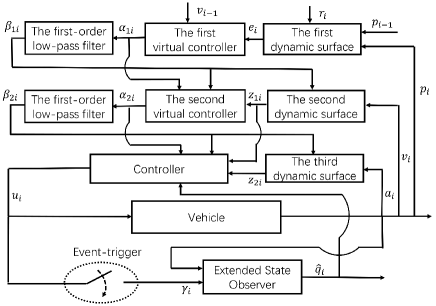
Figure 1: The block diagram of the designed control law.

Therefore, the control law of the each follower vehicle consists of the event-triggered ESO (7), (8), (9) and the controller (3), in which the controller (3) consists of the virtual controllers (15), (17) and the first order low-pass filters (11), (13). It is worth pointing out that the control law of each follower vehicle only uses the information obtained by on-board sensors, such as its own velocity $v_{i}(t)$, acceleration $a_{i}(t)$, the velocity of the preceding vehicle $v_{i-1}(t)$ and the inter-vehicle distance $p_{i-1}(t)-p_{i}(t)$.

4 Stability analysis of vehicle platoon system

We make the following assumptions.

A1. The control input and velocity of the virtual leader vehicle satisfy ${\rm sup}_{t\geq 0}|u_{0}(t)|\leq\overline{u}_{0}$ and ${\rm sup}_{t\geq 0}|v_{0}(t)|\leq\overline{v}_{0}$, where $\overline{u}_{0}>0$ and $\overline{v}_{0}>0$ are known constants.

A2. The external disturbance $\sigma_{i}(t)$ satisfies ${\rm sup}_{t\geq 0}|\sigma_{i}(t)|\leq\sigma_{1i}$. $\sigma_{i}(t)$ is differentiable and $\dot{\sigma}_{i}(t)$ satisfies ${\rm sup}_{t\geq 0}|\dot{\sigma}_{i}(t)|\leq\sigma_{2i}$, where $\sigma_{1i}>0$ and $\sigma_{2i}>0$ are known constants.

A3. The upper and lower bounds of the mass $m_{i}$, total air resistance coefficient $c_{i}$, rolling resistance coefficient $\mu_{i}$ and inertial delay $\tau_{i}$ of the $i$th follower vehicle are known, which are denoted by $\overline{m}_{i},\ \underline{m}_{i},\ \overline{c}_{i},\ \underline{c}_{i},\ \overline{\mu}_{i},\ \underline{\mu}_{i},\ \overline{\tau}_{i},\ \underline{\tau}_{i}$, respectively.

The observation error of the event-triggered ESO is denoted by $e_{1i}(t)=q_{i}(t)-\hat{q}_{i}(t)$. For the boundedness of the observation errors, we have the following lemma.

Lemma 1.

Suppose that Assumptions A2$-$A3 hold. If the differentiation of the unmodeled dynamics $\dot{q}_{i}(t)$ satisfies $|\dot{q}_{i}(t)|\leq c_{1i}+c_{2i}|e_{1i}(t)|+\overline{c}_{bi}l_{i}|e_{1i}(t)|+\overline{c}_{bi}l_{i}\hat{b}_{i}|\psi_{i}(t)|$, the estimation of control gain $\hat{b}_{i}$ satisfies $\max\left\{\underline{b}_{i},\overline{b}_{i}/2\right\}<\hat{b}_{i}\leq\overline{b}_{i}$, the observer gain $l_{i}$ satisfies $l_{i}>(c_{1i}+c_{2i}\overline{e}_{1i})/((1-\overline{c}_{bi})\overline{e}_{1i})$ and the triggering threshold $M_{i}=\overline{e}_{1i}(l_{i}-c_{2i}-\overline{c}_{bi}l_{i})-c_{1i})/(l_{i}\hat{b}_{i}(1+\overline{c}_{bi}))$, then ${\rm sup}_{t\geq 0}|e_{1i}(t)|\leq\overline{e}_{1i}$, where $c_{1i}$ and $c_{2i}$ are positive constants, $\overline{e}_{1i}=|a_{i}(0)|/\tau_{i}+\overline{c}_{i}v_{i}^{2}(0)/(\underline{m}_{i}\underline{\tau}_{i})+g\overline{\mu}_{i}/\underline{\tau}_{i}+\max\{\overline{b}_{i}-\hat{b}_{i},\hat{b}_{i}-\underline{b}_{i}\}|u_{i}(0)|+\sigma_{1i}+|\hat{q}_{i}(0)|$, $\overline{c}_{bi}=\max\left\{(\overline{b}_{i}-\hat{b}_{i})/\hat{b}_{i},(\hat{b}_{i}-\underline{b}_{i})/\hat{b}_{i}\right\}$, $\overline{b}_{i}=1/(\underline{m}_{i}\underline{\tau}_{i})$, $\underline{b}_{i}=1/(\overline{m}_{i}\overline{\tau}_{i})$.

The proof of Lemma 1 is given in Appendix A.

For stability of the vehicle platoon system, we have the following theorem.

Theorem 1.

Suppose that Assumptions A1$-$A3 hold. Consider the system (1) and (2) under the distributed control law which consists of the event-triggered ESO (7), (8), (9) and the controller (3). For any given safe inter-vehicle distance error $\delta\in(0,\min_{i=1,2,...,N}r_{i})$ and control precision $\epsilon\in(0,\delta]$, if the control parameters are designed according to Conditions C1$-$C3, then the string stability and closed-loop stability of the vehicle platoon system are guaranteed, and the Zeno behavior is avoided.

C1. The virtual velocity gain $h_{1i}$ and the virtual acceleration gain $h_{2i}$, $i=1,2,...,N$ satisfy $v_{d,i}^{2}(0)/h_{1i}^{2}+(a_{i}(0)-k_{2i}v_{d,i}(0))^{2}/h_{2i}^{2}\leq\delta^{2}$.

C2. The controller gains $k_{1i}$, $k_{2i}$, $k_{3i}$, $i=1,2,...,N$ satisfy

$$\left\{\begin{aligned} &k_{1i}\geq(3\xi_{i}+\epsilon^{2})/(2\epsilon^{2}),\\ &k_{2i}\geq(3\xi_{i}+\epsilon^{2})/(2\epsilon^{2}),\\ &k_{3i}\geq(3\xi_{i}^{2}h_{2i}^{2}+\overline{e}_{1i}^{2}\epsilon^{2})/(2h_{2i}^{2}\epsilon^{2}\xi_{i}),\end{aligned}\right.$$ (20)

where $\xi_{i}$ is an arbitrarily given positive constant, $i=1,2,...,N$.

C3. The low-pass filter parameters $\kappa_{1i}$, $\kappa_{2i}$, $i=1,2,...,N$ satisfy

$$\left\{\begin{aligned} &\kappa_{1i}\leq(2\xi_{i}\epsilon^{2})/(3\xi_{i}^{2}+\xi_{i}\epsilon^{2}h_{1i}^{2}+\epsilon^{2}\alpha^{2}_{3i}),\\ &\kappa_{2i}\leq(2\xi_{i}\epsilon^{2}h_{1i}^{2})/(3\xi_{i}^{2}h_{1i}^{2}+\xi_{i}\epsilon^{2}h_{2i}^{2}+h_{1i}^{2}\epsilon^{2}\alpha^{2}_{4i}),\end{aligned}\right.$$ (21)

where $\alpha_{3i}=\overline{a}_{i-1}/h_{1i}+\left(2k_{1i}+k_{1i}^{2}/h_{1i}\right)\delta$, $\alpha_{4i}=[(k_{1i}h_{1i}^{2}+k_{2i}h_{1i}^{2}+|h_{1i}/\kappa_{1i}^{2}-h_{1i}^{3}|+|h_{1i}k_{2i}^{2}-h_{1i}^{3}|)/h_{2i}+\alpha_{3i}/\kappa_{1i}+2k_{2i}]\delta$, $\overline{v}_{i}=(2h_{1i}+k_{1i})\delta+\overline{v}_{i-1}$, $\overline{a}_{0}=\max\{a_{i}(0),\overline{u}_{0}\}$, $\overline{a}_{i}=(2h_{2i}+h_{1i}k_{2i}+h_{1i}^{2}+h_{1i}/\kappa_{1i})\delta$.

The proof of Theorem 1 is given in Appendix B. From Theorem 1, it is shown that the control parameters can be properly designed to ensure the stability of the vehicle platoon system provided the disturbance to the leader vehicle $u_{0}(t)$ is bounded.

5 Numerical simulations

Firstly, the vehicle models (1) and (2) are considered. Suppose that there is one virtual leader vehicle and eight follower vehicles in the platoon. The upper and lower bounds of the mass $m_{i}$, inertial delay $\tau_{i}$, total air resistance coefficient $c_{i}$ and rolling resistance coefficient $\mu_{i}$ of the follower vehicles are given by $\overline{m}_{i}=2000\,\rm{kg}$, $\underline{m}_{i}=1500\,\rm{kg}$, $\overline{\tau}_{i}=0.4$,  $\underline{\tau}_{i}=0.2$, $\overline{c}_{i}=0.4$, $\underline{c}_{i}=0.2$, $\overline{\mu}_{i}=0.05$, $\underline{\mu}_{i}=0.02$, $i=1,2,...,8$, respectively. The model parameters of the follower vehicles are randomly generated within the upper and lower bounds given above.

The expected inter-vehicle distances between adjacent vehicles and safe inter-vehicle distance errors are given by $r_{i}=8\,\rm{m}$,   $i=1,2,...,8$ and $\delta=7\,\rm{m}$, respectively. The external disturbances are taken as $\sigma_{i}(t)=\lambda_{1i}e^{-\lambda_{2i}t}+\lambda_{3i}\sin(\lambda_{4i}t)$, where the constants $\lambda_{1i},\lambda_{2i},\lambda_{3i}$ and $\lambda_{4i}$ are randomly generated in $[1\,,20],\ [0.1\,,0.5],\ [0.5\,,1]$ and $[4\,,8]$, respectively. The initial position, velocity and acceleration of the virtual leader vehicle are given by $p_{0}(0)=80\,\rm{m}$, $v_{0}(0)=10\,\rm{m/s}$ and $a_{0}(0)=0\,\rm{m/s^{2}}$, respectively. The initial positions, velocities and accelerations of the follower vehicles are given in Table 1.

Table 1: The initial positions, velocities and accelerations of the follower vehicles.

i	1	2	3	4	5	6	7	8
$p_{i}(0)(\rm{m})$	71	63.5	54	47.2	38.4	30.6	22.1	14.8
$v_{i}(0)(\rm{m/s})$	10	11	11.5	12.5	12.5	11.5	13.5	13
$a_{i}(0)(\rm{m/s^{2}})$	0	1.5	-1	0	-2	1	0	-1

The maneuver of the virtual leader vehicle is divided into three stages. Stage 1 ($t\in[0\,\rm{s},\,6\,s)$): the virtual leader vehicle keeps moving at a constant velocity. Stage 2 ($t\in[6\,\rm{s},\,9\,\rm{s})$): the virtual leader vehicle accelerates, and the expected acceleration of the leader vehicle is generated by CarSim. Specifically, we construct a virtual vehicle in CarSim and then control its throttle opening to accelerate, and record the acceleration. Then we regard the recorded acceleration as the expected acceleration of the virtual leader vehicle. Stage 3 ($t\in[9\,\rm{s},\,15\,\rm{s})$): the virtual leader vehicle continues to move at a constant velocity after accelerating.

Before carrying out the simulations with the designed controller (3), we will show the vehicle platoon maneuver with controller

$$u_{i}(t)=k_{p}e_{i}(t)+k_{v}v_{d,i}(t)+k_{a}a_{i-1}(t)+k_{d}a_{i}(t),$$ (22)

which performs well for the vehicle with linear dynamics (Rajamani & Zhu, 2002). We choose $k_{p}=2000,\ k_{v}=4000,\ k_{a}=2000,\ k_{d}=100$. The evolution of the inter-vehicle distance errors with the controller (22) is shown in Fig. 2.

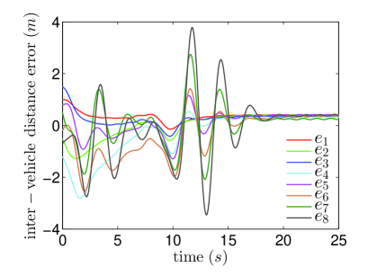
Figure 2: Inter-vehicle distance errors with the controller (22).

Then we preform the simulations with the designed controller (19). For $\epsilon=0.1$, we choose $k_{1i}=0.8,\ k_{2i}=1.5,\ k_{3i}=300,\ \kappa_{1i}=0.05,\ \kappa_{2i}=0.01,\ l_{i}=1200,\ \hat{b}_{i}=0.003,\ h_{1i}=2,\ h_{2i}=8,\ i=1,2,...,8$. The evolution of the inter-vehicle distance errors with $\epsilon=0.1$ is shown in Fig. 3. The actual and the estimated unmodeled dynamics of the 1st and 7th follower vehicles are shown in Fig. 4. The triggering instants of event-triggered ESOs are shown in Fig. 5.

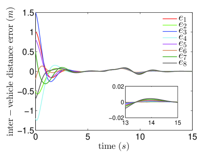
Figure 3: Inter-vehicle distance errors ($\epsilon=0.1$).

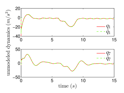
Figure 4: The actual and the estimated unmodeled dynamics of the 1st and 7th follower vehicles.

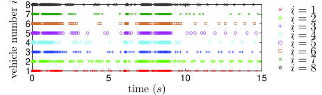
Figure 5: The triggering instants of event-triggered ESOs.

Comparing Fig. 2 and Fig. 3, it can be seen that the controller (3) designed based on the nonlinear vehicle model has better performance than the controller (22). From Fig. 3, it is shown that the inter-vehicle errors gradually decrease from the initial non-zero states and finally converge to a small neighborhood of zero, then the inter-vehicle errors deviate from the steady states due to the acceleration of the leader vehicle. As the acceleration of the leader vehicle becomes zero, the inter-vehicle distance errors converge again. The absolute values of the inter-vehicle distance error $|e_{i}(t)|$ never exceeds the given safe value $\delta$. Fig. 3 shows that the designed control laws can deal with not only the non-zero initial states but also the disturbances to the leader vehicle. It can be seen from Fig. 4 that the unmodeled dynamics in different vehicle models can be estimated well by the event-triggered ESOs. Fig. 5 shows that the event-triggered mechanism can effectively reduce the data transmission from the controller to the ESO.

Then for $\epsilon=0.01$, we choose $k_{1i}=2,\ k_{2i}=8,\ k_{3i}=1000,\ \kappa_{1i}=0.005,\ \kappa_{2i}=0.001,\ l_{i}=1200,\ \hat{b}_{i}=0.003,\ h_{1i}=2,\ h_{2i}=8,\ i=1,2,...,8$. The evolution of the inter-vehicle distance errors with $\epsilon=0.01$ is shown in Fig. 6.

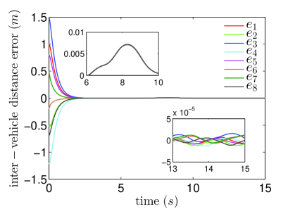
Figure 6: Inter-vehicle distance errors ($\epsilon=0.01$).

It can be seen from Fig. 3 and Fig. 6 that the control precision can be adjusted by properly choosing the control parameters. From Fig. 3 and Fig. 6, we know that the larger controller gains $k_{1i}$, $k_{2i}$, $k_{3i}$ and the smaller filter parameters $\kappa_{1i}$, $\kappa_{2i}$ lead to a faster convergence and reduce the fluctuations of the inter-vehicle distance errors caused by the disturbances to the virtual leader vehicle. However, the larger controller gains may result in larger control inputs when the initial inter-vehicle distance errors are large, which may leads to input saturation, so we need to choose the control parameters with a compromise.

Next, the vehicle models in CarSim are considered and the joint simulations of Simulink and CarSim are carried out. Compared with the nonlinear vehicle models obtained by performing a series of simplifications on the dynamic characteristics of real vehicles, the vehicle models in CarSim are more complex and more consistent with the dynamic characteristics of real vehicles. Firstly, one leader vehicle model and eight follower vehicle models are constructed in CarSim, which are added to the model library of Simulink in the form of S-functions. Then, the joint simulation platform of Simulink and CarSim is built. The constructed vehicle models in CarSim are called by Simulink directly. Similar to the previous simulation, the maneuver of the leader vehicle is divided into three stages. First, the leader vehicle moves at a constant velocity, then slows down, and finally moves at a constant velocity after decelerating. In order to facilitate testing, we develop a graphical user interface (GUI) based on MATLAB. The control parameters can be edited in the GUI directly and the inter-vehicle distance errors can be automatically displayed in the GUI after the program runs. We reselect $k_{1i}=0.9,\ k_{2i}=20,\ k_{3i}=100,\ \kappa_{1i}=0.05,\ \kappa_{2i}=0.005,\ l_{i}=800,\ \hat{b}_{i}=0.05,\ h_{1i}=2,\ h_{2i}=4,\ i=1,2,...,8$. The GUI based on MATLAB is shown in Fig. 7.

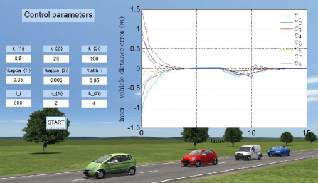
Figure 7: The GUI based on MATLAB.

It can be seen from Fig. 7 that the inter-vehicle distance errors stay within a safe range and eventually converge to a small neighborhood of zero, either with non-zero initial states or with disturbances to the leader vehicle. The joint simulation of Simulink and CarSim shows that although the control laws in this paper are designed for the simplified vehicle models, they are still effective for the more complicated vehicle models in CarSim.

6 Conclusion

We have presented a distributed control law based on an event-triggered ESO and a modified dynamic surface control method for the platoon control of the third-order nonlinear vehicle. The constant spacing policy has been adopted, and the vehicle model with parameter uncertainties and external disturbances has been considered. The control law of each follower vehicle only uses its own velocity, acceleration, the velocity of preceding vehicle and the inter-vehicle distance, which can be obtained by on-board sensors. Firstly, an event-triggered ESO has been designed to estimate the unmodeled dynamics. Then based on the estimate of the unmodeled dynamics, a distributed control law has been proposed by utilizing a modified dynamic surface control method. We have analyzed the stability of the vehicle platoon system and given the range of the control parameters to ensure that the observation errors of the ESOs are bounded and that the string stability and closed-loop stability are guaranteed. We have proved that the Zeno behavior is avoided under the designed event-triggered mechanism.

In this paper, the input delay and the input saturation are not considered. In the future, it is challenging to consider how to design a control law that can deal with the input delay and the input saturation simultaneously.

Appendix A Proof of Lemma 1

Proof of Lemma 1. By (4), (7) and (8), we know

$$\dot{\hat{q}}_{i}(t)= \dot{s}_{i}(t)+l_{i}\dot{a}_{i}(t)$$

$$= -l_{i}s_{i}(t)-l^{2}_{i}a_{i}(t)-l_{i}\hat{b}_{i}\gamma_{i}(t)+l_{i}(q_{i}(t)+\hat{b}_{i}u_{i}(t))$$

$$= l_{i}e_{1i}(t)-l_{i}\hat{b}_{i}\psi_{i}(t).$$ (23)

By (4) and (A), we have the following observation error dynamics

$$\dot{e}_{1i}(t)=-l_{i}e_{1i}(t)+l_{i}\hat{b}_{i}\psi_{i}(t)+w_{i}(t).$$ (24)

Consider the Lyapunov function $V_{ei}(t)=e^{2}_{1i}(t)/2$. By (24), noting that $\left|w_{i}(t)\right|\leq c_{1i}+c_{2i}\left|e_{1i}(t)\right|+\overline{c}_{bi}l_{i}\left|e_{1i}(t)\right|+\overline{c}_{bi}l_{i}\hat{b}_{i}\left|\psi_{i}(t)\right|$, we get

$$\dot{V}_{ei}(t)= -l_{i}e^{2}_{1i}(t)+l_{i}\hat{b}_{i}\psi_{i}(t)e_{1i}(t)+e_{1i}(t)w_{i}(t)$$

$$\leq -l_{i}e^{2}_{1i}(t)+l_{i}\hat{b}_{i}\left|\psi_{i}(t)\right|\left|e_{1i}(t)\right|+\left|e_{1i}(t)\right|\left|w_{i}(t)\right|$$

$$\leq -l_{i}e^{2}_{1i}(t)+c_{2i}e^{2}_{1i}(t)+\overline{c}_{bi}l_{i}e^{2}_{1i}(t)+\left[c_{1i}\right.$$

$$\left.+l_{i}\hat{b}_{i}(1+\overline{c}_{bi})\left|\psi_{i}(t)\right|\right]\left|e_{1i}(t)\right|$$

$$= -2(l_{i}-c_{2i}-\overline{c}_{bi}l_{i})V_{ei}(t)+\sqrt{2}\left[c_{1i}+l_{i}\hat{b}_{i}(1\right.$$

$$\left.+\overline{c}_{bi})\left|\psi_{i}(t)\right|\right]\sqrt{V_{ei}(t)}.$$ (25)

By (A), noting that $\frac{dV_{ei}(t)}{dt}=2\sqrt{V_{ei}(t)}\frac{d\sqrt{V_{ei}(t)}}{dt}$, we obtain

$$\sqrt{V_{ei}(t)}\leq \left(\sqrt{V_{ei}(0)}-A_{i}\right)e^{-\left(l_{i}-c_{2i}-\overline{c}_{bi}l_{i}\right)t}+A_{i},$$ (26)

where$A_{i}=\sqrt{2}[c_{1i}+l_{i}\hat{b}_{i}(1+\overline{c}_{bi})|\psi_{i}(t)|]/[2(l_{i}-c_{2i}-\overline{c}_{bi}l_{i})]$. By (26), noting that $V_{ei}(t)=e_{1i}^{2}(t)/2$, we obtain

$$|e_{1i}(t)|$$

$$= \sqrt{2V_{ei}(t)}$$

$$\leq \left[\sqrt{2V_{ei}(0)}-\sqrt{2}A_{i}\right]e^{-\left(l_{i}-c_{2i}-\overline{c}_{bi}l_{i}\right)t}+\sqrt{2}A_{i}$$

$$= \left(|e_{1i}(0)|-\sqrt{2}A_{i}\right)e^{-\left(l_{i}-c_{2i}-\overline{c}_{bi}l_{i}\right)t}+\sqrt{2}A_{i}.$$ (27)

By $\max\left\{\underline{b}_{i},\overline{b}_{i}/2\right\}<\hat{b}_{i}\leq\overline{b}_{i}$, we know $\overline{c}_{bi}<1$. According to $l_{i}>(c_{1i}+c_{2i}\overline{e}_{1i})/[(1-\overline{c}_{bi})\overline{e}_{1i}]$ and $\overline{c}_{bi}<1$, we have $\overline{e}_{1i}(l_{i}-c_{2i}-\overline{c}_{bi}l_{i})-c_{1i}>0$. By (8) and (9), noting that $M_{i}=\overline{e}_{1i}(l_{i}-c_{2i}-\overline{c}_{bi}l_{i})-c_{1i})/(l_{i}\hat{b}_{i}(1+\overline{c}_{bi}))$, we get $|\psi_{i}(t)|<[\overline{e}_{1i}(l_{i}-c_{2i}-\overline{c}_{bi}l_{i})-c_{1i}]/(l_{i}\hat{b}_{i}(1+\overline{c}_{bi})),\ t\in[t_{k}^{i},t_{k+1}^{i})$. This together with (A) leads to

$$|e_{1i}(t)|\leq\left(|e_{1i}(0)|-\overline{e}_{1i}\right)e^{-\left(l_{i}-c_{2i}-\overline{c}_{bi}l_{i}\right)t}+\overline{e}_{1i}.$$ (28)

From Assumption A2, we get ${\rm sup}_{t\geq 0}|\sigma_{i}(t)|\leq\sigma_{1i}$. By (5), we get $e_{1i}(0)=-a_{i}(0)/\tau_{i}-c_{i}v_{i}^{2}(0)/(m_{i}\tau_{i})-g\mu_{i}/\tau_{i}+(b_{i}-\hat{b}_{i})u_{i}(0)+\sigma_{i}(0)-\hat{q}_{i}(0)$. This together with ${\rm sup}_{t\geq 0}|\sigma_{i}(t)|\leq\sigma_{1i}$ and Assumption A3 leads to $|e_{1i}(0)|\leq\overline{e}_{1i}$. By (28), noting that $|e_{1i}(0)|\leq\overline{e}_{1i}$, we have $|e_{1i}(t)|\leq\overline{e}_{1i},\ \forall\ t\geq 0$. ∎

Appendix B Proof of Theorem 1

Proof of Theorem 1. Choose the following Lyapunov function $V_{i}(t)=(e_{i}^{2}(t)+z_{1i}^{2}(t)+z_{2i}^{2}(t)+\eta_{1i}^{2}(t)+\eta_{2i}^{2}(t))/2$.

By (3), (4), (15)$-$(3), the time derivative of $V_{i}(t)$ is calculated as

$$\dot{V}_{i}(t)$$

$$= -k_{1i}e^{2}_{i}(t)-k_{2i}z^{2}_{1i}(t)-k_{3i}z_{2i}^{2}(t)-\eta_{1i}^{2}(t)/\kappa_{1i}$$

$$-\eta_{2i}^{2}(t)/\kappa_{2i}-h_{1i}e_{i}(t)\eta_{1i}(t)+h_{2i}z_{1i}(t)\eta_{2i}(t)/h_{1i}$$

$$+z_{2i}(t)e_{1i}(t)/h_{2i}-\eta_{1i}(t)\dot{\alpha}_{1i}(t)-\eta_{2i}(t)\dot{\alpha}_{2i}(t)$$

$$\leq -k_{1i}e^{2}_{i}(t)-k_{2i}z^{2}_{1i}(t)-k_{3i}z_{2i}^{2}(t)-\eta^{2}_{1i}(t)/\kappa_{1i}$$

$$-\eta^{2}_{2i}(t)/\kappa_{2i}+h_{1i}|e_{i}(t)||\eta_{1i}(t)|+h_{2i}|z_{1i}(t)||\eta_{2i}(t)|/h_{1i}$$

$$+|z_{2i}(t)||e_{1i}(t)|/h_{2i}+|\eta_{1i}(t)||\dot{\alpha}_{1i}(t)|+|\eta_{2i}(t)||\dot{\alpha}_{2i}(t)|$$

$$\leq -k_{1i}e^{2}_{i}(t)-k_{2i}z^{2}_{1i}(t)-k_{3i}z_{2i}^{2}(t)-\eta^{2}_{1i}(t)/\kappa_{1i}$$

$$-\eta^{2}_{2i}(t)/\kappa_{2i}+e_{i}^{2}(t)/2+h_{1i}^{2}\eta_{1i}^{2}(t)/2+z_{1i}^{2}(t)/2$$

$$+h_{2i}^{2}\eta_{2i}^{2}(t)/(2h_{1i}^{2})+z_{2i}^{2}(t)e_{1i}^{2}(t)/(2h_{2i}^{2}\xi_{i})$$

$$+\eta_{1i}^{2}(t)\dot{\alpha}_{1i}^{2}(t)/(2\xi_{i})+\eta_{2i}^{2}(t)\dot{\alpha}_{2i}^{2}(t)/(2\xi_{i})+3\xi_{i}/2$$

$$= -\left(k_{1i}-1/2\right)e^{2}_{i}(t)-\left(k_{2i}-1/2\right)z^{2}_{1i}(t)$$

$$-\left[k_{3i}-e_{1i}^{2}(t)/(2h_{2i}^{2}\xi_{i})\right]z_{2i}^{2}(t)$$

$$-\left[1/\kappa_{1i}-h_{1i}^{2}/2-\dot{\alpha}^{2}_{1i}(t)/(2\xi_{i})\right]\eta^{2}_{1i}(t)$$

$$-\left[1/\kappa_{2i}-h_{2i}^{2}/(2h_{1i}^{2})-\dot{\alpha}_{2i}^{2}(t)/(2\xi_{i})\right]\eta_{2i}^{2}(t)+3\xi_{i}/2.$$ (29)

Consider the compact set

$$\Omega:=\{(x_{1},x_{2},x_{3},x_{4},x_{5}): x^{2}_{1}/2+x^{2}_{2}/2+x^{2}_{3}/2$$

$$+x^{2}_{4}/2+x^{2}_{5}/2\leq\delta^{2}/2\}.$$

By (10) and (15) , we obtain

$$v_{i}(t)= h_{1i}(z_{1i}(t)+\beta_{1i}(t))$$

$$= h_{1i}z_{1i}(t)+h_{1i}\eta_{1i}(t)+v_{i-1}(t)+k_{1i}e_{i}(t).$$ (30)

From (12) and (17), we know

$$a_{i}(t)= h_{2i}(z_{2i}(t)+\beta_{2i}(t))$$

$$= h_{2i}z_{2i}(t)+h_{2i}\eta_{2i}(t)-h_{1i}k_{2i}z_{1i}(t)$$

$$-h_{1i}\eta_{1i}(t)/\kappa_{1i}+h_{1i}^{2}e_{i}(t).$$ (31)

By (3), (10) and (15), we have

$$\dot{\alpha}_{1i}(t)= (\dot{v}_{i-1}(t)+k_{1i}\dot{e}_{i}(t))/h_{1i}$$

$$= a_{i-1}(t)/h_{1i}-k_{1i}z_{1i}(t)-k_{1i}\eta_{1i}(t)$$

$$-k_{1i}^{2}e_{i}(t)/h_{1i}.$$ (32)

By (10), (13) and (17), we know

$$\dot{\alpha}_{2i}(t)= h_{1i}(-k_{2i}\dot{z}_{1i}(t)-\dot{\eta}_{1i}(t)/\kappa_{1i}+h_{1i}\dot{e}_{i}(t))/h_{2i}$$

$$= -\left(h_{1i}^{2}k_{1i}+h_{1i}^{2}k_{2i}\right)e_{i}(t)/h_{2i}+\dot{\alpha}_{1i}(t)/\kappa_{1i}$$

$$+\left(h_{1i}/\kappa_{1i}^{2}-h_{1i}^{3}\right)\eta_{1i}(t)/h_{2i}-k_{2i}\eta_{2i}(t)$$

$$+\left(h_{1i}k_{2i}^{2}-h_{1i}^{3}\right)z_{1i}(t)/h_{2i}-k_{2i}z_{2i}(t).$$ (33)

According to (4) and (3), we obtain

$$\dot{a}_{i}(t)$$

$$= q_{i}(t)+\hat{b}_{i}u_{i}(t)$$

$$= e_{1i}(t)-(k_{3i}z_{2i}(t)+h_{2i}z_{1i}(t)/h_{1i}+\eta_{2i}(t)/\kappa_{2i})h_{2i}.$$ (34)

By (B) and Assumption A1, we know that $v_{i}(t)$ satisfies $|v_{i}(t)|\leq\overline{v}_{i},\ \forall\ t\geq 0$ on the compact set $\Omega$. By (B), we know that $a_{i}(t)$ satisfies $|a_{i}(t)|\leq\overline{a}_{i},\ \forall\ t\geq 0$ on the compact set $\Omega$. By (B), (B) and Assumption A1 and noting that $|a_{i}(t)|\leq\overline{a}_{i},\ \forall\ t\geq 0$, we obtain that $\dot{\alpha}_{1i}(t)$ and $\dot{\alpha}_{2i}(t)$ satisfy $|\dot{\alpha}_{1i}(t)|\leq\alpha_{3i}$ and $|\dot{\alpha}_{2i}(t)|\leq\alpha_{4i},\ \forall\ t\geq 0$ on the compact set $\Omega$, respectively. From (B), we know that $\dot{a}_{i}(t)$ satisfies $|\dot{a}_{i}(t)|\leq|e_{1i}(t)|+\left(k_{3i}+h_{2i}/h_{1i}+1/\kappa_{2i}\right)h_{2i}\delta$ on the compact set $\Omega$.

By (4), (11)$-$(3) and (A), we know $\dot{u}_{i}(t)=h_{2i}[-(l_{i}+k_{3i})e_{1i}(t)/h_{2i}+l_{i}\hat{b}_{i}\psi_{i}(t)/h_{2i}-h_{2i}e_{i}(t)+(k_{2i}+k_{3i})h_{2i}z_{1i}(t)/h_{1i}+(k_{3i}^{2}-h_{2i}^{2}/h_{1i}^{2})z_{2i}(t)-(h_{2i}^{2}/h_{1i}^{2}-1/\kappa_{2i}^{2})\eta_{2i}(t)+\dot{\alpha}_{2i}(t)/\kappa_{2i}]/\hat{b}_{i}$. This together with $|\dot{\alpha}_{2i}(t)|\leq\alpha_{4i},\ \forall\ t\geq 0$ leads to

$$|\dot{u}_{i}(t)|$$

$$\leq h_{2i}\left[(l_{i}+k_{3i})|e_{1i}(t)|/h_{2i}+l_{i}\hat{b}_{i}|\psi_{i}(t)|/h_{2i}+h_{2i}\delta\right.$$

$$\left.+(k_{2i}+k_{3i})h_{2i}\delta/h_{1i}+\left|k_{3i}^{2}-h_{2i}^{2}/h_{1i}^{2}\right|\delta\right.$$

$$\left.+\left|h_{2i}^{2}/h_{1i}^{2}-1/\kappa_{2i}^{2}\right|\delta+\alpha_{4i}/\kappa_{2i}\right]/\hat{b}_{i}.$$ (35)

From Assumption A2, we know ${\rm sup}_{t\geq 0}|\dot{\sigma}_{i}(t)|\leq\sigma_{2i}$. By (6), (B) and Assumption A3, noting that ${\rm sup}_{t\geq 0}|\dot{\sigma}_{i}(t)|\leq\sigma_{2i}$, $|v_{i}(t)|\leq\overline{v}_{i}$, $|a_{i}(t)|\leq\overline{a}_{i}$ and $|\dot{a}_{i}(t)|\leq|e_{1i}(t)|+\left(k_{3i}+h_{2i}/h_{1i}+1/\kappa_{2i}\right)h_{2i}\delta$, we know

$$|w_{i}(t)|$$

$$\leq |\dot{a}_{i}(t)|/\tau_{i}+2c_{i}|v_{i}(t)||a_{i}(t)|/(m_{i}\tau_{i})+2c_{i}|v_{i}(t)||\dot{a}_{i}(t)|$$

$$/m_{i}+2c_{i}a_{i}^{2}(t)/m_{i}+|(b_{i}-\hat{b}_{i})/\hat{b}_{i}||\dot{u}_{i}(t)|+|\dot{\sigma}_{i}(t)|$$

$$\leq \left(1/\underline{\tau}_{i}+2\overline{c}_{i}\overline{v}_{i}/\underline{m}_{i}\right)\left[|e_{1i}(t)|+\left(k_{3i}+h_{2i}/h_{1i}+1/\kappa_{2i}\right)\right.$$

$$\left.\times h_{2i}\delta\right]+2\overline{c}_{i}\overline{v}_{i}\overline{a}_{i}/(\underline{m}_{i}\underline{\tau}_{i})+2\overline{c}_{i}\overline{a}_{i}^{2}/\underline{m}_{i}+\sigma_{2i}$$

$$+|(b_{i}-\hat{b}_{i})/\hat{b}_{i}|\left[(l_{i}+k_{3i})|e_{1i}(t)|+l_{i}\hat{b}_{i}|\psi_{i}(t)|+h_{2i}^{2}\delta\right.$$

$$\left.+(k_{2i}+k_{3i})h_{2i}^{2}\delta/h_{1i}+|k_{3i}^{2}-h_{2i}^{2}/h_{1i}^{2}|\delta+\alpha_{4i}/\kappa_{2i}\right.$$

$$\left.+\left|h_{2i}^{2}/h_{1i}^{2}-1/\kappa_{2i}^{2}\right|\delta\right].$$ (36)

Denote $c_{bi}=(b_{i}-\hat{b}_{i})/\hat{b}_{i}$. By $\max\left\{\underline{b}_{i},\overline{b}_{i}/2\right\}<\hat{b}_{i}\leq\overline{b}_{i}$, we know $|c_{bi}|\leq\overline{c}_{bi}$ and $\overline{c}_{bi}<1$. From (B), noting that $|\dot{a}_{i}(t)|\leq|e_{1i}(t)|+\left(k_{3i}+h_{2i}/h_{1i}+1/\kappa_{2i}\right)h_{2i}\delta$, we obtain

$$\left|w_{i}(t)\right|\leq c_{1i}+c_{2i}\left|e_{1i}(t)\right|+\overline{c}_{bi}l_{i}\left|e_{1i}(t)\right|+\overline{c}_{bi}l_{i}\hat{b}_{i}\left|\psi_{i}(t)\right|,$$

where $c_{1i}=(1/\underline{\tau}_{i}+2\overline{c}_{i}\overline{v}_{i}/\underline{m}_{i})(k_{3i}+h_{2i}/h_{1i}+1/\kappa_{2i})h_{2i}\delta+2\overline{c}_{i}\overline{v}_{i}\overline{a}_{i}/(\underline{m}_{i}\underline{\tau}_{i})+2\overline{c}_{i}\overline{a}_{i}^{2}/\underline{m}_{i}+\sigma_{2i}+\overline{c}_{bi}[(h_{2i}^{2}+(k_{2i}+k_{3i})h_{2i}^{2}/h_{1i}+|k_{3i}^{2}-h_{2i}^{2}/h_{1i}^{2}|+|h_{2i}^{2}/h_{1i}^{2}-1/\kappa_{2i}^{2}|)\delta+\alpha_{4i}/\kappa_{2i}]$, $c_{2i}=1/\underline{\tau}_{i}+2\overline{c}_{i}\overline{v}_{i}/\underline{m}_{i}+\overline{c}_{bi}k_{3i}$. This together with $\dot{q}_{i}(t)=w_{i}(t)$ and Lemma 1 leads to $|e_{1i}(t)|\leq\overline{e}_{1i},\ \forall\ t\geq 0$. From (B), noting that $|e_{1i}(t)|\leq\overline{e}_{1i}$, $|\dot{\alpha}_{1i}(t)|\leq\alpha_{3i}$ and $|\dot{\alpha}_{2i}(t)|\leq\alpha_{4i},\ \forall\ t\geq 0$, we obtain

$$\dot{V}_{i}(t)$$

$$\leq -\left(k_{1i}-1/2\right)e^{2}_{i}(t)-\left(k_{2i}-1/2\right)z^{2}_{1i}(t)$$

$$-\left[k_{3i}-\overline{e}_{1i}^{2}/(2h_{2i}^{2}\xi_{i})\right]z_{2i}^{2}(t)$$

$$-\left[1/\kappa_{1i}-h_{1i}^{2}/2-\alpha^{2}_{3i}/(2\xi_{i})\right]\eta^{2}_{1i}(t)$$

$$-\left[1/\kappa_{2i}-h_{2i}^{2}/(2h_{1i}^{2})-\alpha_{4i}^{2}/(2\xi_{i})\right]\eta_{2i}^{2}(t)+3\xi_{i}/2.$$ (37)

Denote $\rho_{i}=\min\{k_{1i}-1/2,\ k_{2i}-1/2,\ k_{3i}-\overline{e}_{1i}^{2}/(2h_{2i}^{2}\xi_{i}),\\ \ 1/\kappa_{1i}-h_{1i}^{2}/2-\alpha^{2}_{3i}/(2\xi_{i}),\ 1/\kappa_{2i}-h_{2i}^{2}/(2h_{1i}^{2})-\alpha_{4i}^{2}/(2\xi_{i})\}$. This together with (B) leads to

$$\dot{V}_{i}(t) \leq-2\rho_{i}V_{i}(t)+3\xi_{i}/2.$$ (38)

From (38), we get

$$V_{i}(t) \leq V_{i}(0)e^{-2\rho_{i}t}+3\xi_{i}(1-e^{-2\rho_{i}t})/(4\rho_{i}).$$ (39)

By (11) and (13), we know $\eta_{1i}(0)=0$ and $\eta_{2i}(0)=0$, which leads to $V_{i}(0)=e_{i}^{2}(0)/2+z_{1i}^{2}(0)/2+z_{2i}^{2}(0)/2$. By (10)$-$(13), (15) and (17), we know $z_{1i}(0)=(-v_{d,i}(0)-k_{1i}e_{i}(0))/h_{1i}$ and $z_{2i}(0)=(a_{i}(0)-k_{2i}v_{d,i}(0)-(k_{1i}k_{2i}+h_{1i}^{2})e_{i}(0))/h_{2i}$. This together with $V_{i}(0)=e_{i}^{2}(0)/2+z_{1i}^{2}(0)/2+z_{2i}^{2}(0)/2$ leads to

$$V_{i}(0)=(A_{0i}e_{i}^{2}(0)+B_{0i}e_{i}(0)+C_{0i})/2.$$ (40)

From (40), we know that if

$$|e_{i}(0)|\leq\min\{|(-B_{0i}+(B_{0i}^{2}-4A_{0i}C_{0i})^{1/2})/(2A_{0i})|,$$

$$|(-B_{0i}-(B_{0i}^{2}-4A_{0i}C_{0i})^{1/2})/(2A_{0i})|\}$$

then $V_{i}(0)\leq\delta^{2}/2$, where $A_{0i}=1+k_{1i}^{2}/h_{1i}^{2}+(k_{1i}k_{2i}+h_{1i}^{2})^{2}/h_{2i}^{2}$, $B_{0i}=2k_{1i}v_{di}(0)/h_{1i}^{2}-2(a_{i}(0)-k_{2i}v_{di}(0))(k_{1i}k_{2i}+h_{1i}^{2})/h_{2i}^{2}$, $C_{0i}=v_{di}^{2}(0)/h_{1i}^{2}+(a_{i}(0)-k_{2i}v_{di}(0))^{2}/h_{2i}^{2}-\delta^{2}$.

From (20) and (21), we know $\rho_{i}\geq 3\xi_{i}/(2\epsilon^{2})$. This together with $\epsilon\leq\delta$ leads to $\rho_{i}\geq 3\xi_{i}/(2\delta^{2})$. From (39), noting that $V_{i}(0)\leq\delta^{2}/2$ and $\rho_{i}\geq 3\xi_{i}/(2\delta^{2})$, we know $V_{i}(t)\leq\delta^{2}/2,\ \forall\ t>0$, which means $\max_{i=1,2,...,N}\sup_{t>0}|e_{i}(t)|\leq\delta$, so the string stability is guaranteed.

From (39) and $\rho_{i}\geq 3\xi_{i}/(2\epsilon^{2})$, we know $\limsup_{t\to\infty}V_{i}(t)\leq(3\xi_{i})/(4\rho_{i})\leq\epsilon^{2}/2$, which means $\limsup_{t\to\infty}|e_{i}(t)|\leq\epsilon$, so the closed-loop stability is guaranteed.

From (B), noting that $|e_{1i}(t)|\leq\overline{e}_{1i}$, we know

$$|\dot{u}_{i}(t)|\leq l_{i}|\psi_{i}(t)|+B_{i},$$ (41)

where $B_{i}=h_{2i}[(l_{i}+k_{3i})\overline{e}_{1i}/h_{2i}+(h_{2i}+(k_{2i}+k_{3i})h_{2i}/h_{1i}+|k_{3i}^{2}-h_{2i}^{2}/h_{1i}^{2}|+|h_{2i}^{2}/h_{1i}^{2}-1/\kappa_{2i}^{2}|+\alpha_{4i}/\kappa_{2i})\delta]/\hat{b}_{i}$. From (8), we know $\psi_{i}(t)=\gamma_{i}(t)-u_{i}(t)=u_{i}(t_{k}^{i})-u_{i}(t)=-\int_{t_{k}^{i}}^{t}\dot{u}_{i}(\tau)\,d\tau,\ t\in[t_{k}^{i},t_{k+1}^{i})$. This together with (41) leads to $|\psi_{i}(t)|\leq\int_{t_{k}^{i}}^{t}|\dot{u}_{i}(\tau)|\,d\tau\leq\int_{t_{k}^{i}}^{t}l_{i}\left|\psi_{i}(\tau)\right|+B_{i}\,d\tau<\int_{t_{k}^{i}}^{t}l_{i}M_{i}+B_{i}\,d\tau=(t-t_{k}^{i})(l_{i}M_{i}+B_{i}),\ t\in[t_{k}^{i},t_{k+1}^{i})$. Then we know that $|\psi_{i}(t)|<M_{i}$ when $t=t_{k}^{i}+M_{i}/(l_{i}M_{i}+B_{i})$. According to (8) and (9), we get $t_{k+1}^{i}-t_{k}^{i}>M_{i}/(l_{i}M_{i}+B_{i})$, so there exists a positive low bound of the time interval of the event triggering, and the Zeno behavior is avoided under the designed event-trigged mechanism.∎

References

Chehardoli & Ghasemi (2018)
Chehardoli, H., & Ghasemi, A.
(2018).
Adaptive centralized/decentralized control and
identification of 1-d heterogeneous vehicular platoons based on constant time
headway policy.
IEEE Transactions on Intelligent
Transportation Systems, 19,
3376–3386.
Di Bernardo et al. (2014)
Di Bernardo, M., Salvi, A., &
Santini, S. (2014).
Distributed consensus strategy for platooning of
vehicles in the presence of time-varying heterogeneous communication delays.
IEEE Transactions on Intelligent
Transportation Systems, 16,
102–112.
Eyre et al. (1998)
Eyre, J., Yanakiev, D., &
Kanellakopoulos, I. (1998).
A simplified framework for string stability analysis
of automated vehicles?
Vehicle System Dynamics, 30, 375–405.
Ge et al. (2021)
Ge, X., Han, Q., Zhang,
X., & Ding, D. (2021).
Dynamic event-triggered control and estimation: A
survey.
International Journal of Automation and
Computing, 18, 857–886.
Guanetti et al. (2018)
Guanetti, J., Kim, Y., &
Borrelli, F. (2018).
Control of connected and automated vehicles: State of
the art and future challenges.
Annual Reviews in Control, 45, 18–40.
Guo & Yue (2012)
Guo, G., & Yue, W. (2012).
Autonomous platoon control allowing range-limited
sensors.
IEEE Transactions on Vehicular Technology,
61, 2901–2912.
Guo et al. (2017a)
Guo, X., Wang, J., Liao,
F., & Teo, R. S. H. (2017a).
Cnn-based distributed adaptive control for
vehicle-following platoon with input saturation.
IEEE Transactions on Intelligent
Transportation Systems, 19,
3121–3132.
Guo et al. (2017b)
Guo, X., Wang, J., Liao,
F., & Xiao, W. (2017b).
Adaptive platoon control for nonlinear vehicular
systems with asymmetric input deadzone and inter-vehicular spacing
constraints.
In 2017 IEEE 56th Annual Conference on
Decision and Control (CDC) (pp. 393–398).
IEEE.
Han (2009)
Han, J. (2009).
From pid to active disturbance rejection control.
IEEE Transactions on Industrial
Electronics, 56, 900–906.
Hao & Barooah (2013)
Hao, H., & Barooah, P.
(2013).
Stability and robustness of large platoons of
vehicles with double-integrator models and nearest neighbor interaction.
International Journal of Robust and Nonlinear
Control, 23, 2097–2122.
Jovanovic & Bamieh (2005)
Jovanovic, M. R., & Bamieh, B.
(2005).
On the ill-posedness of certain vehicular platoon
control problems.
IEEE Transactions on Automatic Control,
50, 1307–1321.
Kwon & Chwa (2014)
Kwon, J. W., & Chwa, D.
(2014).
Adaptive bidirectional platoon control using a
coupled sliding mode control method.
IEEE Transactions on Intelligent
Transportation Systems, 15,
2040–2048.
Li & Guo (2020)
Li, D., & Guo, G. (2020).
Prescribed performance concurrent control of
connected vehicles with nonlinear third-order dynamics.
IEEE Transactions on Vehicular Technology,
69, 14793–14802.
Li et al. (2015)
Li, S. E., Zheng, Y., Li,
K., & Wang, J. (2015).
An overview of vehicular platoon control under the
four-component framework.
In 2015 IEEE Intelligent Vehicles Symposium
(IV) (pp. 286–291).
IEEE.
Liu et al. (2021)
Liu, A., Li, T., Gu, Y.,
& Dai, H. (2021).
Cooperative extended state observer based control of
vehicle platoons with arbitrarily small time headway.
Automatica, 129.
Miskowicz (2018)
Miskowicz, M. (2018).
Event-based control and signal processing.
CRC press.
Naus et al. (2010)
Naus, G. J., Vugts, R. P.,
Ploeg, J., van De Molengraft, M. J., &
Steinbuch, M. (2010).
String-stable cacc design and experimental
validation: A frequency-domain approach.
IEEE Transactions on Vehicular Technology,
59, 4268–4279.
Öncü et al. (2014)
Öncü, S., Ploeg, J.,
Van de Wouw, N., & Nijmeijer, H.
(2014).
Cooperative adaptive cruise control: Network-aware
analysis of string stability.
IEEE Transactions on Intelligent
Transportation Systems, 15,
1527–1537.
Ploeg et al. (2013)
Ploeg, J., Van De Wouw, N., &
Nijmeijer, H. (2013).
Lp string stability of cascaded systems: Application
to vehicle platooning.
IEEE Transactions on Control Systems
Technology, 22, 786–793.
Rajamani & Zhu (2002)
Rajamani, R., & Zhu, C.
(2002).
Semi-autonomous adaptive cruise control systems.
IEEE Transactions on Vehicular Technology,
51, 1186–1192.
Sheikholeslam & Desoer (1993)
Sheikholeslam, S., & Desoer, C. A.
(1993).
Longitudinal control of a platoon of vehicles with no
communication of lead vehicle information: A system level study.
IEEE Transactions on Vehicular Technology,
42, 546–554.
Swaroop et al. (2000)
Swaroop, D., Hedrick, J. K.,
Yip, P. P., & Gerdes, J. C.
(2000).
Dynamic surface control for a class of nonlinear
systems.
IEEE Transactions on Automatic Control,
45, 1893–1899.
Willke et al. (2009)
Willke, T. L., Tientrakool, P., &
Maxemchuk, N. F. (2009).
A survey of inter-vehicle communication protocols and
their applications.
IEEE Communications Surveys & Tutorials,
11, 3–20.
Wu et al. (2016)
Wu, Y., Li, S. E., Zheng,
Y., & Hedrick, J. K. (2016).
Distributed sliding mode control for multi-vehicle
systems with positive definite topologies.
In 2016 IEEE 55th Conference on Decision and
Control (CDC) (pp. 5213–5219).
IEEE.
Xiao & Gao (2011)
Xiao, L., & Gao, F.
(2011).
Practical string stability of platoon of adaptive
cruise control vehicles.
IEEE Transactions on Intelligent
Transportation Systems, 12,
1184–1194.
Yue & Guo (2012)
Yue, W., & Guo, G. (2012).
Guaranteed cost adaptive control of nonlinear
platoons with actuator delay.
Journal of Dynamic Systems, Measurement, and
Control, 134.
Zheng et al. (2016)
Zheng, Y., Li, S. E., Li,
K., Borrelli, F., & Hedrick, J. K.
(2016).
Distributed model predictive control for
heterogeneous vehicle platoons under unidirectional topologies.
IEEE Transactions on Control Systems
Technology, 25, 899–910.
Zheng et al. (2015)
Zheng, Y., Li, S. E.,
Wang, J., Cao, D., &
Li, K. (2015).
Stability and scalability of homogeneous vehicular
platoon: Study on the influence of information flow topologies.
IEEE Transactions on Intelligent
Transportation Systems, 17,
14–26.
Zhu & Zhu (2018)
Zhu, Y., & Zhu, F. (2018).
Distributed adaptive longitudinal control for
uncertain third-order vehicle platoon in a networked environment.
IEEE Transactions on Vehicular Technology,
67, 9183–9197.
Zhu & Zhu (2019)
Zhu, Y., & Zhu, F. (2019).
Barrier-function-based distributed adaptive control
of nonlinear cavs with parametric uncertainty and full-state constraint.
Transportation Research Part C: Emerging
Technologies, 104, 249–264.