The colored Jones polynomial
of the figure-eight knot
and a quantum modularity

Abstract.

We study the asymptotic behavior of the $N$-dimensional colored Jones polynomial of the figure-eight knot evaluated at $\exp\bigl{(}(u+2p\pi\sqrt{-1})/N\bigr{)}$, where $u$ is a small real number and $p$ is a positive integer. We show that it is asymptotically equivalent to the product of the $p$-dimensional colored Jones polynomial evaluated at $\exp\bigl{(}4N\pi^{2}/(u+2p\pi\sqrt{-1})\bigr{)}$ and a term that grows exponentially with growth rate determined by the Chern–Simons invariant. This indicates a quantum modularity of the colored Jones polynomial.

1. Introduction

Let $K$ be an oriented knot in the three-sphere $S^{3}$. For a positive integer $N$, we denote by $J_{N}(K;q)$ the colored Jones polynomial associated with the irreducible $N$-dimensional representation of the Lie algebra $\mathfrak{sl}(2;\mathbb{C})$. Here we normalize $J_{N}(K;q)$ so that $J_{N}(U;q)=1$ for the unknot $U$.

Let us consider an evaluation $J_{N}\left(K;e^{2\pi\sqrt{-1}/N}\right)$. It is well known that it coincides with Kashaev’s invariant $\langle K\rangle_{N}$ [12, 25]. R. Kashaev conjectured that his invariant grows exponentially as $N\to\infty$, and that its growth rate gives the hyperbolic volume of the knot complement when $K$ is a hyperbolic knot, that is, $S^{3}\setminus{K}$ possesses a (unique) complete hyperbolic structure with finite volume [13]. In [25], Kashaev’s conjecture was generalized to any knot replacing the hyperbolic volume with simplicial volume (also known as Gromov’s norm [8]).

Conjecture 1.1 (Volume conjecture).

Let $K\subset S^{3}$ be any knot. Then we have

$$\lim_{N\to\infty}\frac{1}{N}\log\bigl{|}J_{N}(K;e^{2\pi\sqrt{-1}/N})\bigr{|}=\frac{1}{2\pi}\operatorname{Vol}(S^{3}\setminus{K}),$$

where $\operatorname{Vol}(S^{3}\setminus{K})$ is the simplicial volume of $S^{3}\setminus{K}$.

So far, Kashaev’s conjecture is proved for the figure-eight knot by T. Ekholm, and for knots with up to seven crossings [31, 33, 32]. The volume conjecture is proved for hyperbolic knots with up to seven crossings as above, for all the torus knots by Kashaev and O. Tirkkonen [14], for the Whitehead doubles of the torus knots by H. Zheng [37], and the $(2,2k+1)$-cable of the figure-eight knot by T. Le and A. Tran [18].

J. Murakami, M. Okamoto, T. Takata, Y. Yokota, and the author complexified Kashaev’s conjecture as follows [26, Conjecture 1.2]:

Conjecture 1.2.

For a hyperbolic knot $K$ in $S^{3}$, we have

$$J_{N}(K;e^{2\pi\sqrt{-1}/N})\underset{N\to\infty}{\sim}\frac{N}{2\pi}\operatorname{CV}(K),$$

where $\operatorname{CV}(K):=\operatorname{Vol}(S^{3}\setminus{K})+\sqrt{-1}\operatorname{CS}^{\mathrm{SO}(3)}(S^{3}\setminus{K})$ is the complex volume with $\operatorname{CS}^{\mathrm{SO}(3)}$ the $\mathrm{SO}(3)$ Chern–Simons invariant [21].

For a hyperbolic knot $K\subset S^{3}$, let $\rho\colon\pi_{1}(S^{3}\setminus{K})\to\mathrm{SL}(2;\mathbb{C})$ be an irreducible representation that is a small deformation of the holonomy representation corresponding to the complete hyperbolic structure. Note that $\rho$ corresponds to an incomplete hyperbolic structure [35]. Up to conjugation, we may assume that $\rho$ sends the meridian of $K$ to $\begin{pmatrix}e^{u/2}&\ast\\ 0&e^{-u/2}\end{pmatrix}$ and the preferred longitude to $\begin{pmatrix}-e^{v(u)/2}&\ast\\ 0&-e^{-v(u)/2}\end{pmatrix}$ (see for example [30]). Associated with $u$, we can define the $\mathrm{SL}(2;\mathbb{C})$ Chern–Simons invariant $\operatorname{CS}_{u,v(u)}(\rho)$ and the cohomological adjoint Reidemeister torsion $T_{K}(u)$. See [29, Chapter 5] for example. Note that in [29] we define the homological adjoint Reidemeister torsion (it is called the twisted Reidemeister torsion there). So we need to take its inverse to define the cohomological torsion. Note also that $\operatorname{Vol}(S^{3}\setminus{K})+\sqrt{-1}\operatorname{CS}^{\mathrm{SO}(3)}(S^{3}\setminus{K})$ in Conjecture 1.2 coincides with $\sqrt{-1}\operatorname{CS}_{0,0}(\rho_{0})$ for a hyperbolic knot $K$ with holonomy representation $\rho_{0}$.

In [28], Yokota and the author proved that for the figure-eight knot $E$, the limit $\lim_{N\to\infty}\frac{1}{N}\log J_{N}\left(E;e^{(u+2\pi\sqrt{-1})/N}\right)$ exists if the complex number $u$ is in a small neighborhood of $0$ (and not a rational multiple of $\pi\sqrt{-1}$). Moreover the limit determines the holomorphic function $f(u)$ introduced in [30, Theorem 2]. In other words, the asymptotic behavior of $J_{N}(E;e^{(u+2\pi\sqrt{-1})/N})$ determines the $\mathrm{SL}(2;\mathbb{C})$ Chern–Simons invariant associated with $u$.

For a general hyperbolic knot $K$, the following conjecture was proposed in [24] (see also [2, 9]).

Conjecture 1.3.

Let $K\subset S^{3}$ be a hyperbolic knot. Then there exists a neighborhood $U\subset\mathbb{C}$ of $0$ such that if $u\in U\setminus\pi\sqrt{-1}\mathbb{Q}$, then we have

$$J_{N}\left(K;e^{(u+2\pi\sqrt{-1})/N}\right)\\ \underset{N\to\infty}{\sim}\frac{\sqrt{-\pi}}{2\sinh(u/2)}T_{K}(u)^{1/2}\left(\frac{N}{u+2\pi\sqrt{-1}}\right)^{1/2}\exp\left(\frac{N\times S_{K}(u)}{u+2\pi\sqrt{-1}}\right),$$

where $T_{K}(u)$ is the cohomological adjoint Reidemeister torsion, and $\operatorname{CS}_{u,v(u)}(\rho)=S_{K}(u)-u\pi\sqrt{-1}-\frac{1}{4}uv(u)$ is the Chern–Simons invariant, both associated with $u$.

In [24], we proved that the conjecture is true for the figure-eight knot and a positive real number $u<\operatorname{arccosh}(3/2)$.

In this paper, we study the colored Jones polynomial of the figure-eight knot evaluated at $q=\exp\bigl{(}(u+2p\pi\sqrt{-1})/N\bigr{)}$ for a real number $u$ with $0<u<\operatorname{arccosh}(3/2)$ and a positive integer $p$. We will show

Theorem 1.4.

Let $E$ be the figure-eight knot and put $\xi:=u+2p\pi\sqrt{-1}$. Then we have

(1.1) $$J_{N}\left(E;e^{\xi/N}\right)\\ =\frac{\sqrt{-\pi}}{2\sinh(u/2)}T_{E}(u)^{1/2}J_{p}\left(E;e^{4N\pi^{2}/\xi}\right)\left(\frac{N}{\xi}\right)^{1/2}e^{\frac{N}{\xi}\times S_{E}(u)}\bigl{(}1+O(N^{-1})\bigr{)}$$

as $N\to\infty$, where we put

$$S_{E}(u) :=\operatorname{Li}_{2}\left(e^{-u-\varphi(u)}\right)-\operatorname{Li}_{2}\left(e^{-u+\varphi(u)}\right)+u\bigl{(}\varphi(u)+2\pi\sqrt{-1}\bigr{)},$$

$$T_{E}(u) :=\frac{2}{\sqrt{(2\cosh{u}+1)(2\cosh{u}-3)}}.$$

Here $\operatorname{Li}_{2}(z):=-\int_{0}^{z}\frac{\log(1-w)}{w}\,dw$ is the dilogarithm function and we put

$$\varphi(u):=\log\left(\cosh{u}-\frac{1}{2}-\frac{1}{2}\sqrt{(2\cosh{u}+1)(2\cosh{u}-3)}\right).$$

Remark 1.5.

The case where $p=1$ was proved in [24].

Remark 1.6.

When $p=0$, the author proved that for the figure-eight knot $E$, $J_{N}\left(E;e^{u/N}\right)$ converges to $1/\Delta(E;e^{u})$, where $\Delta(K;t)$ is the Alexander polynomial of a knot $K$ normalized so that $\Delta(K;t)=\Delta(K;t^{-1})$ and $\Delta(U;t)=1$ [23]. Soon after, it was generalized by S. Garoufalidis and T. Le to any knot in $S^{3}$. See [5, 4, 6].

As a corollary we have the following asymptotic equivalence.

Corollary 1.7.

We have

(1.2) $$\frac{J_{N}\left(E;e^{\xi/N}\right)}{J_{p}\left(E;e^{4N\pi^{2}/\xi}\right)}\underset{N\to\infty}{\sim}\frac{\sqrt{-\pi}}{2\sinh(u/2)}T_{E}(u)^{1/2}\left(\frac{N}{\xi}\right)^{1/2}e^{\frac{N}{\xi}\times S_{E}(u)}.$$

This indicates a quantum modularity for the colored Jones polynomial.

Conjecture (Conjecture 7.3).

Let $K$ be a hyperbolic knot. For a small complex number $u$ that is not a rational multiple of $\pi\sqrt{-1}$, and positive integers $p$ and $N$, put $\xi:=u+2p\pi\sqrt{-1}$ and $X:=\frac{2N\pi\sqrt{-1}}{\xi}$. Then for any $\eta=\begin{pmatrix}a&b\\ c&d\end{pmatrix}\in\mathrm{SL}(2;\mathbb{Z})$ with $c>0$, the following asymptotic equivalence holds.

$$\frac{J_{cN+dp}\left(K;e^{2\pi\sqrt{-1}\eta(X)}\right)}{J_{p}\left(K;e^{2\pi\sqrt{-1}X}\right)}\underset{N\to\infty}{\sim}C_{K,\eta}(u)\frac{\sqrt{-\pi}}{2\sinh(u/2)}\left(\frac{T_{K}(u)}{\hbar_{\eta}(X)}\right)^{1/2}\exp\left(\frac{S_{K}(u)}{\hbar_{\eta}(X)}\right)$$

for $C_{K,\eta}(u)\in\mathbb{C}$ that does not depend on $p$, where we put $\eta(X):=\frac{aX+b}{cX+d}$ and $\hbar_{\eta}(X):=\frac{2c\pi\sqrt{-1}}{cX+d}$.

Compare it with Zagier’s quantum modularity conjecture for Kashaev’s invariant [36].

Conjecture (Conjecture 7.1).

Let $K$, $\eta$, $N$, and $p$ as above. If we put $X_{0}:=\frac{N}{p}$, the following holds.

$$\frac{J_{cN+dp}\left(K;e^{2\pi\sqrt{-1}\eta(X_{0})}\right)}{J_{p}\left(K;e^{2\pi\sqrt{-1}X_{0}}\right)}\\ \underset{N\to\infty}{\sim}C_{K,\eta}\left(\frac{2\pi}{\hbar_{\eta}(X_{0})}\right)^{3/2}\exp\left(\frac{\sqrt{-1}\operatorname{CV}(K)}{\hbar_{\eta}(X_{0})}\right),$$

where $C_{K,\eta}$ is a complex number depending only on $\eta$ and $K$.

The paper is organized as follows.

In Section 2, we define the colored Jones polynomial and introduce a quantum dilogarithm. We express the colored Jones polynomial as a sum of the quantum dilogarithms assuming $(p,N)=1$ in Section 3. In Section 4, we approximate it by using the dilogarithm function by using the fact that the quantum dilogarithm converges to the dilogarithm. We use the Poisson summation formula á la Ohtsuki [31] to replace the sum with an integral in Section 5. In Section 6, we prove the main theorem (Theorem 1.4). We discuss a quantum modularity of the colored Jones polynomial in Section 7. Section 8 is devoted to proofs of lemmas used in the other sections. In Appendix, we calculate the colored Jones polynomial in the case where $(p,N)\neq 1$.

2. Preliminaries

Let $J_{N}(K;q)$ be the $N$-dimensional colored Jones polynomial of $K\subset S^{3}$ associated with the $N$-dimensional irreducible representation of the Lie algebra $\mathfrak{sl}_{2}(\mathbb{C})$, where $N$ is a positive integer and $q$ is a complex parameter [16, 34, 15]. It is normalized so that $J_{N}(U;q)=1$ for the unknot $U$. In particular, $J_{2}(K;q)$ is (a version) of the original Jones polynomial [11]. More precisely, $J_{2}(K;q)$ satisfies the following skein relation:

$$qJ_{2}\left(\raisebox{-5.12149pt}{\includegraphics[scale={0.1}]{positive.eps}};q\right)-q^{-1}J_{2}\left(\raisebox{-5.12149pt}{\includegraphics[scale={0.1}]{negative.eps}};q\right)=\left(q^{1/2}-q^{-1/2}\right)J_{2}\left(\raisebox{-5.12149pt}{\includegraphics[scale={0.1}]{null.eps}};q\right).$$

K. Habiro [10, P. 36 (1)] (see also [19, Theorem 5.1]) and T. Le [17, 1.2.2. Example, P. 129] gave a simple formula for the colored Jones polynomial of the figure-eight knot $E$ as follows:

(2.1) $$J_{N}(E;q) =\sum_{k=0}^{N-1}\prod_{l=1}^{k}\left(q^{(N+l)/2}-q^{-(N+l)/2}\right)\left(q^{(N-l)/2}-q^{-(N-l)/2}\right)$$

(2.2) $$=\sum_{k=0}^{N-1}q^{-kN}\prod_{l=1}^{k}\left(1-q^{N+l}\right)\left(1-q^{N-l}\right).$$

For a real number $u$ with $0<u<\kappa:=\operatorname{arccosh}(3/2)=0.962424\dots$, and a positive integer $p$, we put $\xi:=u+2p\pi\sqrt{-1}$. Then we have

(2.3) $$J_{N}\left(E;e^{\xi/N}\right)=\sum_{k=0}^{N-1}e^{-k\xi}\prod_{l=1}^{k}\left(1-e^{(N+l)\xi/N}\right)\left(1-e^{(N-l)\xi/N}\right).$$

We want to replace the products in (2.3) with some values of a continuous function. To do that we introduce a so-called quantum dilogarithm following [3].

Put $\mathrel{\mathop{\mathbb{R}}\limits^{\vbox to0.0pt{\kern-1.0pt\hbox{$\scriptstyle\frown$}\vss}}}:=(-\infty,-1]\cup\{z\in\mathbb{C}\mid|z|=1,\operatorname{Im}{z}\geq 0\}\cup[1,\infty)$ and orient it from left to right. We consider the integral $\int_{\mathrel{\mathop{\mathbb{R}}\limits^{\vbox to0.0pt{\kern-1.0pt\hbox{$\scriptstyle\frown$}\vss}}}}\frac{e^{(2z-1)x}}{x\sinh(x)\sinh(\gamma x)}\,dx$, where $\gamma:=\frac{\xi}{2N\pi\sqrt{-1}}$.

Lemma 2.1.

The integral $\int_{\mathrel{\mathop{\mathbb{R}}\limits^{\vbox to0.0pt{\kern-1.0pt\hbox{$\scriptstyle\frown$}\vss}}}}\frac{e^{(2z-1)x}}{x\sinh(x)\sinh(\gamma x)}\,dx$ converges if $-p/(2N)<\operatorname{Re}{z}<1+p/(2N)$.

A proof is given in § 8. Note that the poles of the integrand is

$$\{x\in\mathbb{C}\mid x=k\pi\sqrt{-1}\;\;\text{($k\in\mathbb{Z}$)}\}\cup\{x\in\mathbb{C}\mid x=l\pi\sqrt{-1}/\xi\;\;\text{($l\in\mathbb{Z}$)}\}$$

and so $\mathrel{\mathop{\mathbb{R}}\limits^{\vbox to0.0pt{\kern-1.0pt\hbox{$\scriptstyle\frown$}\vss}}}$ avoids the poles.

We define

$$T_{N}(z):=\frac{1}{4}\int_{\mathrel{\mathop{\mathbb{R}}\limits^{\vbox to0.0pt{\kern-1.0pt\hbox{$\scriptstyle\frown$}\vss}}}}\frac{e^{(2z-1)x}}{x\sinh(x)\sinh(\gamma x)}\,dx.$$

We also consider three related integrals $\int_{\mathrel{\mathop{\mathbb{R}}\limits^{\vbox to0.0pt{\kern-1.0pt\hbox{$\scriptstyle\frown$}\vss}}}}\frac{e^{(2z-1)x}}{x^{k}\sinh(x)}\,dx$ ($k=0,1,2$), which converge if $0<\operatorname{Re}{z}<1$ by similar reasons to Lemma 2.1.

Definition 2.2.

We put

$$\mathcal{L}_{0}(z) :=\int_{\mathrel{\mathop{\mathbb{R}}\limits^{\vbox to0.0pt{\kern-1.0pt\hbox{$\scriptstyle\frown$}\vss}}}}\frac{e^{(2z-1)x}}{\sinh(x)}\,dx,$$

$$\mathcal{L}_{1}(z) :=\frac{-1}{2}\int_{\mathrel{\mathop{\mathbb{R}}\limits^{\vbox to0.0pt{\kern-1.0pt\hbox{$\scriptstyle\frown$}\vss}}}}\frac{e^{(2z-1)x}}{x\sinh(x)}\,dx,$$

$$\mathcal{L}_{2}(z) :=\frac{\pi\sqrt{-1}}{2}\int_{\mathrel{\mathop{\mathbb{R}}\limits^{\vbox to0.0pt{\kern-1.0pt\hbox{$\scriptstyle\frown$}\vss}}}}\frac{e^{(2z-1)x}}{x^{2}\sinh(x)}\,dx$$

for $z$ with $0<\operatorname{Re}{z}<1$.

Their derivatives are given as follows.

$$\frac{d\,\mathcal{L}_{2}(z)}{d\,z} =-2\pi\sqrt{-1}\mathcal{L}_{1}(z),$$

$$\frac{d\,\mathcal{L}_{1}(z)}{d\,z} =-\mathcal{L}_{0}(z).$$

We also have the following lemma.

Lemma 2.3.

If $0<\operatorname{Re}{z}<1$, then we have

$$\mathcal{L}_{0}(z) =\frac{-2\pi\sqrt{-1}}{1-e^{-2\pi\sqrt{-1}z}},$$

$$\mathcal{L}_{1}(z) =\log\left(1-e^{2\pi\sqrt{-1}z}\right),$$

$$\mathcal{L}_{2}(z) =\operatorname{Li}_{2}\left(e^{2\pi\sqrt{-1}z}\right).$$

Here we use the branch of $\log{w}$ so that $-\pi<\operatorname{Im}\log{w}\leq\pi$ and $\operatorname{Li}_{2}(w)$ has branch cut at $(1,\infty)$.

Proof.

As [27, Lemma 2.5], we can prove the following equalities:

$$\mathcal{L}_{0}(z) =\frac{-2\pi\sqrt{-1}}{1-e^{-2\pi\sqrt{-1}z}},$$

$$\mathcal{L}_{1}(z) =\begin{cases}\log\left(1-e^{2\pi\sqrt{-1}z}\right)&\text{if $\operatorname{Im}{z}\geq 0$},\\ \pi\sqrt{-1}(2z-1)+\log\left(1-e^{-2\pi\sqrt{-1}z}\right)&\text{if $\operatorname{Im}{z}<0$},\end{cases}$$

$$\mathcal{L}_{2}(z) =\begin{cases}\operatorname{Li}_{2}\left(e^{2\pi\sqrt{-1}z}\right)&\text{if $\operatorname{Im}{z}\geq 0$},\\ \frac{\pi^{2}}{3}(6z^{2}-6z+1)-\operatorname{Li}_{2}\left(e^{-2\pi\sqrt{-1}z}\right)&\text{if $\operatorname{Im}{z}<0$}.\end{cases}$$

So we need to prove the lemma for the case where $\operatorname{Im}{z}<0$.

There is nothing to prove for $\mathcal{L}_{0}(z)$.

If $0<\operatorname{Re}{z}<1$, then using the identity (see for example [20])

(2.4) $$\operatorname{Li}_{2}(w^{-1})=-\operatorname{Li}_{2}(w)-\frac{\pi^{2}}{6}-\frac{1}{2}\bigl{(}\log(-w)\bigr{)}^{2},$$

we have

$$\operatorname{Li}_{2}\left(e^{-2\pi\sqrt{-1}z}\right) =-\operatorname{Li}_{2}\left(e^{2\pi\sqrt{-1}z}\right)-\frac{\pi^{2}}{6}-\frac{1}{2}\bigl{(}2\pi\sqrt{-1}z-\pi\sqrt{-1}\bigr{)}^{2}$$

$$=-\operatorname{Li}_{2}\left(e^{2\pi\sqrt{-1}z}\right)+2\pi^{2}z^{2}+\frac{\pi^{2}}{3},$$

where we use the fact that $0<\operatorname{Im}(2\pi\sqrt{-1}z)<2\pi$. Therefore we have

$$\mathcal{L}_{2}(z)=-\operatorname{Li}_{2}\left(e^{-2\pi\sqrt{-1}z}\right)+\frac{\pi^{2}}{3}\bigl{(}6z^{2}-6z+1\bigr{)}=\operatorname{Li}_{2}\left(e^{2\pi\sqrt{-1}z}\right)$$

as required.

As for $\mathcal{L}_{1}(z)$, since $\log\left(e^{\pi\sqrt{-1}(2z-1)}\right)=2\pi\sqrt{-1}z-\pi\sqrt{-1}$, we have

$$\log\left(1-e^{-2\pi\sqrt{-1}z}\right)+\pi\sqrt{-1}(2z-1) =\log\left(1-e^{-2\pi\sqrt{-1}z}\right)+\log\left(e^{\pi\sqrt{-1}(2z-1)}\right)$$

$$=\log\left(1-e^{2\pi\sqrt{-1}z}\right),$$

completing the proof. ∎

We can prove that $T_{N}(z)$ converges to $\frac{N}{\xi}\operatorname{Li}_{2}\left(e^{2\pi\sqrt{-1}z}\right)$. More precisely we have

Lemma 2.4.

For any positive real number $M$ and a sufficiently small positive real number $\nu$, we have

$$T_{N}(z)=\frac{N}{\xi}\operatorname{Li}_{2}\left(e^{2\pi\sqrt{-1}z}\right)+O(1/N)$$

as $N\to\infty$ in the region

$$\{z\in\mathbb{C}\mid\nu\leq\operatorname{Re}{z}\leq 1-\nu,|\operatorname{Im}{z}|\leq M\}.$$

In particular $T_{N}(z)$ uniformly converges to $\frac{N}{\xi}\operatorname{Li}_{2}\left(e^{2\pi\sqrt{-1}z}\right)$ in the region above.

A proof is also given in § 8.

The following lemma is essential in the paper. Put $E_{N}(z):=e^{T_{N}(z)}$.

Lemma 2.5.

If $0<\operatorname{Re}{z}<1$, then we have

$$\frac{E_{N}(z-\gamma/2)}{E_{N}(z+\gamma/2)}=1-e^{2\pi\sqrt{-1}z}.$$

Proof.

Recalling that $\gamma=\frac{\xi}{2N\pi\sqrt{-1}}$, we have

$$T_{N}(z-\gamma/2)-T_{N}(z+\gamma/2) =\frac{1}{4}\int_{\mathrel{\mathop{\mathbb{R}}\limits^{\vbox to0.0pt{\kern-1.0pt\hbox{$\scriptstyle\frown$}\vss}}}}\frac{e^{(2z-\gamma-1)x}-e^{(2z+\gamma-1)x}}{x\sinh(x)\sinh(\gamma x)}\,dx$$

$$=-\int_{\mathrel{\mathop{\mathbb{R}}\limits^{\vbox to0.0pt{\kern-1.0pt\hbox{$\scriptstyle\frown$}\vss}}}}\frac{e^{(2z-1)x}}{2x\sinh(x)}\,dx=\mathcal{L}_{1}(z).$$

Taking the exponentials of both sides, the lemma follows from Lemma 2.3. ∎

As a corollary, we have

Corollary 2.6.

Let $n$ be an integer. If $nN/p<j<(n+1)N/p$, we have

$$\frac{E_{N}\bigl{(}(j-1/2)\gamma-n\bigr{)}}{E_{N}\bigl{(}(j+1/2)\gamma-n\bigr{)}} =1-e^{2j\gamma\pi\sqrt{-1}},$$

and

$$\frac{E_{N}\bigl{(}n+1-(j+1/2)\gamma\bigr{)}}{E_{N}\bigl{(}n+1-(j-1/2)\gamma\bigr{)}} =1-e^{-2j\gamma\pi\sqrt{-1}}.$$

Proof.

Since $\operatorname{Re}\gamma=p/N$, we have $0<\operatorname{Re}(j\gamma-n)<1$. Therefore putting $z:=j\gamma-n$ in Lemma 2.5, we have the first equality. Similarly, putting $z:=n+1-j\gamma$, we have the second equality. ∎

We prepare other two lemmas.

Lemma 2.7.

For a complex number $w$ with $|\operatorname{Re}{w}|<\operatorname{Re}\gamma$, we have

$$\frac{E_{N}\bigl{(}w+\gamma/2\bigr{)}}{E_{N}\bigl{(}w-\gamma/2+1\bigr{)}}=\frac{1-e^{2\pi\sqrt{-1}w/\gamma}}{1-e^{2\pi\sqrt{-1}w}}.$$

Proof.

By definition, we have

$$T_{N}(w+\gamma/2)-T_{N}(w-\gamma/2+1)$$

$$= \frac{1}{4}\int_{\mathrel{\mathop{\mathbb{R}}\limits^{\vbox to0.0pt{\kern-1.0pt\hbox{$\scriptstyle\frown$}\vss}}}}\frac{e^{(2w+\gamma-1)t}-e^{(2w-\gamma+1)t}}{t\sinh(t)\sinh(\gamma t)}\,dt$$

$$= \frac{1}{2}\int_{\mathrel{\mathop{\mathbb{R}}\limits^{\vbox to0.0pt{\kern-1.0pt\hbox{$\scriptstyle\frown$}\vss}}}}\frac{e^{2wt}\cosh(t)}{t\sinh(t)}\,dt-\frac{1}{2}\int_{\mathrel{\mathop{\mathbb{R}}\limits^{\vbox to0.0pt{\kern-1.0pt\hbox{$\scriptstyle\frown$}\vss}}}}\frac{e^{2wt}\cosh(\gamma t)}{t\sinh(\gamma t)}\,dt$$

$$= \frac{1}{4}\int_{\mathrel{\mathop{\mathbb{R}}\limits^{\vbox to0.0pt{\kern-1.0pt\hbox{$\scriptstyle\frown$}\vss}}}}\frac{e^{(2w+1)t}}{t\sinh(t)}\,dt+\frac{1}{4}\int_{\mathrel{\mathop{\mathbb{R}}\limits^{\vbox to0.0pt{\kern-1.0pt\hbox{$\scriptstyle\frown$}\vss}}}}\frac{e^{(2w-1)t}}{t\sinh(t)}\,dt$$

$$-\frac{1}{4}\int_{\mathrel{\mathop{\mathbb{R}}\limits^{\vbox to0.0pt{\kern-1.0pt\hbox{$\scriptstyle\frown$}\vss}}}}\frac{e^{(2w+\gamma)t}}{t\sinh(\gamma t)}\,dt-\frac{1}{4}\int_{\mathrel{\mathop{\mathbb{R}}\limits^{\vbox to0.0pt{\kern-1.0pt\hbox{$\scriptstyle\frown$}\vss}}}}\frac{e^{(2w-\gamma)t}}{t\sinh(\gamma t)}\,dt$$

$$= -\frac{1}{2}\mathcal{L}_{1}(w+1)-\frac{1}{2}\mathcal{L}_{1}(w)+\frac{1}{2}\mathcal{L}_{1}(w/\gamma+1)+\frac{1}{2}\mathcal{L}_{1}(w/\gamma).$$

Taking the exponentials, we have the lemma from Lemma 2.3. ∎

Lemma 2.8.

For a complex number $z$ with $|\operatorname{Re}{z}|<\operatorname{Re}\gamma/2$, we have

$$\frac{E_{N}(z)}{E_{N}(z+1)}=1+e^{2\pi\sqrt{-1}z/\gamma}.$$

Proof.

By definition, we have

$$T_{N}(z)-T_{N}(z+1)$$

$$= \frac{1}{4}\int_{\mathrel{\mathop{\mathbb{R}}\limits^{\vbox to0.0pt{\kern-1.0pt\hbox{$\scriptstyle\frown$}\vss}}}}\frac{e^{(2z-1)t}-e^{(2z+1)t}}{t\sinh(t)\sinh(\gamma t)}\,dt$$

$$= -\frac{1}{2}\int_{\mathrel{\mathop{\mathbb{R}}\limits^{\vbox to0.0pt{\kern-1.0pt\hbox{$\scriptstyle\frown$}\vss}}}}\frac{e^{2zt}}{t\sinh(\gamma t)}\,dt$$

$$= -\frac{1}{2}\int_{\gamma\mathrel{\mathop{\mathbb{R}}\limits^{\vbox to0.0pt{\kern-1.0pt\hbox{$\scriptstyle\frown$}\vss}}}}\frac{e^{2zs/\gamma}}{s\sinh(s)}\,ds$$

$$= \mathcal{L}_{1}(z/\gamma+1/2).$$

Taking the exponentials, we get the lemma from Lemma 2.3. ∎

3. Summation

In this section, we express $J_{N}\left(E;e^{\xi/N}\right)$ in terms of the quantum dilogarithm $T_{N}(z)$.

We assume that $p$ and $N$ are coprime. See Appendix for the case with $(p,N)\neq 1$.

If $k<N/p$, then from Corollary 2.6 with $(j,n)=(N-l,p-1)$ and $(j,n)=(N+l,p)$, we have

$$\prod_{l=1}^{k}(1-e^{(N-l)\xi/N})(1-e^{(N+l)\xi/N})$$

$$= \prod_{l=1}^{k}(1-e^{2(N-l)\gamma\pi\sqrt{-1}})(1-e^{2(N+l)\gamma\pi\sqrt{-1}})$$

$$= \prod_{l=1}^{k}\frac{E_{N}\bigl{(}(N-l-1/2)\gamma-p+1\bigr{)}}{E_{N}\bigl{(}(N-l+1/2)\gamma-p+1\bigr{)}}$$

$$\times\prod_{l=1}^{k}\frac{E_{N}\bigl{(}(N+l-1/2)\gamma-p\bigr{)}}{E_{N}\bigl{(}(N+l+1/2)\gamma-p\bigr{)}}$$

$$= \frac{E_{N}\bigl{(}(N-k-1/2)\gamma-p+1\bigr{)}}{E_{N}\bigl{(}(N-1/2)\gamma-p+1\bigr{)}}\frac{E_{N}\bigl{(}(N+1/2)\gamma-p\bigr{)}}{E_{N}\bigl{(}(N+k+1/2)\gamma-p\bigr{)}}$$

$$= \frac{1-e^{4p\pi^{2}N/\xi}}{1-e^{\xi}}\times\frac{E_{N}\bigl{(}(N-k-1/2)\gamma-p+1\bigr{)}}{E_{N}\bigl{(}(N+k+1/2)\gamma-p\bigr{)}},$$

where we use Lemma 2.7 with $w=N\gamma-p$ in the last equality.

Similarly, if $k$ satisfies $mN/p<k<(m+1)N/p$, then we have

(3.1) $$\prod_{l=1}^{k}(1-e^{(N-l)\xi/N})(1+e^{(N+l)\xi/N})$$

$$= \prod_{j=0}^{m-1}\left(\prod_{l=\lfloor jN/p\rfloor+1}^{\lfloor(j+1)N/p\rfloor}\frac{E_{N}\bigl{(}(N-l-1/2)\gamma-p+j+1\bigr{)}}{E_{N}\bigl{(}(N-l+1/2)\gamma-p+j+1\bigr{)}}\right.$$

$$\left.\phantom{\prod_{j=0}^{m-1}\Bigl{(}}\times\prod_{l=\lfloor jN/p\rfloor+1}^{\lfloor(j+1)N/p\rfloor}\frac{E_{N}\bigl{(}(N+l-1/2)\gamma-p-j\bigr{)}}{E_{N}\bigl{(}(N+l+1/2)\gamma-p-j\bigr{)}}\right)$$

$$\times\prod_{l=\lfloor mN/p\rfloor+1}^{k}\frac{E_{N}\bigl{(}(N-l-1/2)\gamma-p+m+1\bigr{)}}{E_{N}\bigl{(}(N-l+1/2)\gamma-p+m+1\bigr{)}}$$

$$\times\prod_{l=\lfloor mN/p\rfloor+1}^{k}\frac{E_{N}\bigl{(}(N+l-1/2)\gamma-p-m\bigr{)}}{E_{N}\bigl{(}(N+l+1/2)\gamma-p-m\bigr{)}}$$

$$= \prod_{j=0}^{m-1}\frac{E_{N}\bigl{(}(N-\lfloor(j+1)N/p\rfloor-1/2)\gamma-p+j+1\bigr{)}}{E_{N}\bigl{(}(N-\lfloor jN/p\rfloor-1/2)\gamma-p+j+1\bigr{)}}$$

$$\times\prod_{j=0}^{m-1}\frac{E_{N}\bigl{(}(N+\lfloor jN/p\rfloor+1/2)\gamma-p-j\bigr{)}}{E_{N}\bigl{(}(N+\lfloor(j+1)N/p\rfloor+1/2)\gamma-p-j\bigr{)}}$$

$$\times\frac{E_{N}\bigl{(}(N-k-1/2)\gamma-p+m+1\bigr{)}}{E_{N}\bigl{(}(N-\lfloor mN/p\rfloor-1/2)\gamma-p+m+1\bigr{)}}$$

$$\times\frac{E_{N}\bigl{(}(N+\lfloor mN/p\rfloor+1/2)\gamma-p-m\bigr{)}}{E_{N}\bigl{(}(N+k+1/2)\gamma-p-m\bigr{)}}$$

$$= \frac{1-e^{4pN\pi^{2}/\xi}}{1-e^{\xi}}\left(\prod_{j=1}^{m}\left(1-e^{4(p-j)N\pi^{2}/\xi}\right)\left(1-e^{4(p+j)N\pi^{2}/\xi}\right)\right)$$

$$\times\frac{E_{N}\bigl{(}(N-k-1/2)\gamma-p+m+1\bigr{)}}{E_{N}\bigl{(}(N+k+1/2)\gamma-p-m\bigr{)}},$$

where we use Lemma 2.7 with $w=N\gamma-p$, and Lemma 2.8 with $z=(N-\lfloor lN/p\rfloor-1/2)\gamma-p+l$ and $z=(N+\lfloor lN/p\rfloor+1/2)\gamma-p-l$ ($l=1,2,\dots,m$).

Remark 3.1.

Since $\operatorname{Re}{\gamma}=p/N$, we have $\operatorname{Re}\bigl{(}(N-\lfloor lN/p\rfloor-1/2)\gamma-p+l\bigr{)}=-\frac{p}{N}\lfloor\frac{lN}{p}\rfloor-\frac{p}{2N}+l$. Since $lN/p$ is not an integer, we have $lN/p-1<\lfloor lN/p\rfloor<lN/p$ (the equality $\lfloor lN/p\rfloor=lN/p$ does not hold). So $\left|\operatorname{Re}\bigl{(}(N-\lfloor lN/p\rfloor-1/2)\gamma-p+l\bigr{)}\right|<\operatorname{Re}{\gamma}/2$ and the assumption of Lemma 2.8 holds.

Therefore, from (2.3) we have

(3.2) $$J_{N}\left(E;e^{\xi/N}\right)$$

$$= \sum_{m=0}^{p-1}\sum_{mN/p<k<(m+1)N/p}e^{-k\xi}\prod_{l=1}^{k}\left(1-e^{(N+l)\xi/N}\right)\left(1-e^{(N-l)\xi/N}\right)$$

$$= \frac{1-e^{4pN\pi^{2}/\xi}}{1-e^{\xi}}\sum_{m=0}^{p-1}\left(\prod_{j=1}^{m}\left(1-e^{4(p-j)N\pi^{2}/\xi}\right)\left(1-e^{4(p+j)N\pi^{2}/\xi}\right)\right.$$

$$\times\left.\vphantom{\sum_{m=0}^{p-1}}\sum_{mN/p<k<(m+1)N/p}e^{-k\xi}\frac{E_{N}\bigl{(}(N-k-1/2)\gamma-p+m+1\bigr{)}}{E_{N}\bigl{(}(N+k+1/2)\gamma-p-m\bigr{)}}\right)$$

$$= \frac{1-e^{-4pN\pi^{2}/\xi}}{2\sinh(u/2)}$$

$$\quad\times\sum_{m=0}^{p-1}\left(\beta_{p,m}\sum_{mN/p<k<(m+1)N/p}\exp\left(N\times f_{N}\left(\frac{2k+1}{2N}-\frac{2m\pi\sqrt{-1}}{\xi}\right)\right)\right),$$

where we put

$$\beta_{p,m} :=e^{-4mpN\pi^{2}/\xi}\prod_{j=1}^{m}\left(1-e^{4(p-j)N\pi^{2}/\xi}\right)\left(1-e^{4(p+j)N\pi^{2}/\xi}\right),$$

(3.3) $$f_{N}(z) :=\frac{1}{N}T_{N}\left(\frac{\xi(1-z)}{2\pi\sqrt{-1}}-p+1\right)-\frac{1}{N}T_{N}\left(\frac{\xi(1+z)}{2\pi\sqrt{-1}}-p\right)$$

$$\quad-uz+\frac{4p\pi^{2}}{\xi}.$$

Remark 3.2.

Since we have

$$\operatorname{Re}\left(\frac{\xi(1\pm z)}{2\pi\sqrt{-1}}\right)=p(1\pm\operatorname{Re}{z})\pm\frac{u}{2\pi}\operatorname{Im}{z},$$

the function $f_{N}(z)$ is defined in the region

$$\left\{z\in\mathbb{C}\Bigm{|}-\frac{1}{2N}<\frac{u}{2p\pi}\operatorname{Im}{z}+\operatorname{Re}{z}<\frac{1}{p}+\frac{1}{2N}\right\}$$

from Lemma 2.1.

4. Approximation

In the previous section, we express $J_{N}\left(E;e^{\xi/N}\right)$ as a sum of the function $f_{N}(z)$. In this section, we approximate it by using a function that does not depend on $N$.

Since $T_{N}(z)/N$ uniformly converges to $\operatorname{Li}_{2}\left(e^{2\pi\sqrt{-1}z}\right)/\xi$ (Lemma 2.4), $f_{N}(z)$ uniformly converges to

$$F(z):=\frac{1}{\xi}\operatorname{Li}_{2}\left(e^{\xi(1-z)}\right)-\frac{1}{\xi}\operatorname{Li}_{2}\left(e^{\xi(1+z)}\right)-uz+\frac{4p\pi^{2}}{\xi}$$

in the region

(4.1) $$\left\{z\in\mathbb{C}\Bigm{|}\frac{\nu}{p}\leq\operatorname{Re}{z}+\frac{u}{2p\pi}\operatorname{Im}{z}\leq\frac{1}{p}-\frac{\nu}{p},\left|\operatorname{Re}{z}-\frac{2p\pi}{u}\operatorname{Im}{z}\right|\leq\frac{2M\pi}{u}+1\right\}.$$

By using the identity (2.4), if $z$ is in the region

$$U_{0}:=\left\{z\in\mathbb{C}\Bigm{|}0<\operatorname{Re}{z}+\frac{u}{2p\pi}\operatorname{Im}{z}<\frac{1}{p}\right\},$$

we have

$$\operatorname{Li}_{2}\left(e^{\xi(1-z)}\right) =-\operatorname{Li}_{2}\left(e^{-\xi(1-z)}\right)-\frac{\pi^{2}}{6}-\frac{1}{2}\left(\log\left(-e^{-\xi(1-z)}\right)\right)^{2}$$

$$=-\operatorname{Li}_{2}\left(e^{-\xi(1-z)}\right)-\frac{\pi^{2}}{6}-\frac{1}{2}(-\xi(1-z)+(2p-1)\pi\sqrt{-1})^{2}$$

since $\operatorname{Im}\xi(1-z)=2p\pi-(uy+2p\pi x)$. Similarly, we have

$$\operatorname{Li}_{2}\left(e^{\xi(1+z)}\right) =-\operatorname{Li}_{2}\left(e^{-\xi(1+z)}\right)-\frac{\pi^{2}}{6}-\frac{1}{2}\left(\log\left(-e^{-\xi(1+z)}\right)\right)^{2}$$

$$=-\operatorname{Li}_{2}\left(e^{-\xi(1+z)}\right)-\frac{\pi^{2}}{6}-\frac{1}{2}(-\xi(1+z)+(2p+1)\pi\sqrt{-1})^{2}$$

since $\operatorname{Im}\xi(1+z)=2p\pi+(uy+2p\pi x)$. Therefore, $F(z)$ can also be written as

$$F(z)=\frac{1}{\xi}\operatorname{Li}_{2}\left(e^{-\xi(1+z)}\right)-\frac{1}{\xi}\operatorname{Li}_{2}\left(e^{-\xi(1-z)}\right)+uz-2\pi\sqrt{-1}$$

in $U_{0}$.

The first derivative of $F(z)$ is

(4.2) $$\frac{d}{d\,z}F(z)=\log\left(1-e^{-u-\xi z}\right)+\log\left(1-e^{-u+\xi z}\right)+u=\log\left(e^{u}+e^{-u}-e^{\xi z}-e^{-\xi z}\right)$$

because $-\pi<\arg\left(1-e^{-u-\xi z)}\right)+\arg\left(1-e^{-u+\xi z)}\right)<\pi$ when $u$ is real from the lemma below. Here we choose the branch of $\arg$ so that $-\pi<\arg\zeta\leq\pi$ for any $\zeta\in\mathbb{C}$. Note that $e^{\pm\xi z}\in\mathbb{R}$ if and only if $\operatorname{Im}(\xi z)=u\operatorname{Im}{z}+2p\pi\operatorname{Re}{z}=2k\pi$ for some $k\in\mathbb{Z}$, which implies that if $z\in U_{0}$ then $e^{\pm\xi z}\not\in\mathbb{R}$.

Lemma 4.1.

Let $a$ be a positive real number, and $w$ be a complex number with $w\not\in\mathbb{R}$. Then we have $-\pi<\arg(1-aw)+\arg(1-aw^{-1})<\pi$.

Proof.

We may assume that $\operatorname{Im}{w}>0$ without loss of generality. Then we can easily see that $-\pi<\arg(1-aw)<0$ and that $0<\arg(1-aw^{-1})<\pi$, which implies the result. ∎

The second derivative of $F(z)$ equals

$$\frac{d^{2}}{d\,z^{2}}F(z)=\frac{\xi\left(e^{-\xi z}-e^{\xi z}\right)}{e^{u}+e^{-u}-e^{\xi z}-e^{-\xi z}}.$$

Now, define

(4.3) $$\varphi(u):=\log\left(\cosh{u}-\frac{1}{2}-\frac{1}{2}\sqrt{(2\cosh{u}+1)(2\cosh{u}-3)}\right),$$

where we take the square root as a positive multiple of $\sqrt{-1}$, recalling that $\cosh{u}<3/2$. Note that $\varphi(u)$ satisfies the equality

$$e^{u}+e^{-u}-e^{\varphi(u)}-e^{-\varphi(u)}=1.$$

Lemma 4.2.

If $0<u<\kappa=\operatorname{arccosh}(3/2)$, then $\varphi(u)$ is purely imaginary with $-\pi/3<\operatorname{Im}\varphi(u)<0$.

Proof.

First note that $e^{\varphi(u)}$ is a solution to the following quadratic equation:

$$x^{2}-(2\cosh{u}-1)x+1=0.$$

Therefore $\left|e^{\varphi(u)}\right|=1$ and we conclude that $\varphi(u)$ is purely imaginary. Put $\theta:=\operatorname{Im}\varphi(u)$.

Since $0<u<\kappa$, we see that $1<2\cosh{u}-1<2$. Then since $e^{-\theta\sqrt{-1}}$ is the other solution to the quadratic equation above, we have $2\cos\theta=2\cosh{u}-1$. Therefore we see that $-\pi/3<\theta<0$ because the argument of $\log$ in (4.3) is in the fourth quadrant. ∎

As in the proof above, we put $\theta:=\operatorname{Im}\varphi(u)$. We also put $\sigma_{0}:=\frac{(\theta+2\pi)\sqrt{-1}}{\xi}$. Since we have

$$\operatorname{Re}\sigma_{0}+\frac{u}{2p\pi}\operatorname{Im}\sigma_{0}=\frac{\theta+2\pi}{2p\pi}$$

and $0>\theta>-\pi/3$, we see that $\sigma_{0}\in U_{0}$.

We have

$$\frac{d}{d\,z}F(\sigma_{0})=\log\left(e^{u}+e^{-u}-e^{\varphi(u)}-e^{-\varphi(u)}\right)=0.$$

We also have

$$\frac{d^{2}}{d\,z^{2}}F(\sigma_{0})=\xi\sqrt{(2\cosh{u}+1)(2\cosh{u}-3)}.$$

Therefore we conclude that $F(z)$ is of the form

(4.4) $$F(z)=F(\sigma_{0})+a_{2}(z-\sigma_{0})^{2}+a_{3}(z-\sigma_{0})^{3}+a_{4}(z-\sigma_{0})^{4}+\cdots$$

with $a_{2}:=\frac{1}{2}\xi\sqrt{(2\cosh{u}+1)(2\cosh{u}-3)}$.

Now, the sum

(4.5) $$\sum_{m/p<k/N<(m+1)/p}\exp\left(N\times f_{N}\left(\frac{2k+1}{2N}-\frac{2m\pi\sqrt{-1}}{\xi}\right)\right)$$

can be approximate by the sum

$$\sum_{m/p<k/N<(m+1)/p}\exp\left(N\times\Phi_{m}\left(\frac{2k+1}{2N}\right)\right),$$

where we put

$$\Phi_{m}(z):=F\left(z-\frac{2m\pi\sqrt{-1}}{\xi}\right).$$

Moreover, in the next section we approximate the sum (4.5) by the integral $N\int_{m/p}^{(m+1)/p}e^{N\Phi_{m}(z)}\,dz$.

Note that the function $\Phi_{m}(z)$ is defined in the region

$$U_{m}:=\left\{z\in\mathbb{C}\Bigm{|}\frac{m}{p}<\operatorname{Re}{z}+\frac{u}{2p\pi}\operatorname{Im}{z}<\frac{m+1}{p}\right\}.$$

Put $\sigma_{m}:=\sigma_{0}+\frac{2m\pi\sqrt{-1}}{\xi}$. Then we see that

$$\operatorname{Re}{\sigma_{m}}+\frac{u}{2p\pi}\operatorname{Im}{\sigma_{m}}=\operatorname{Re}{\sigma_{0}}+\frac{u}{2p\pi}\operatorname{Im}{\sigma_{0}}+\frac{m}{p}=\frac{\theta+2(m+1)\pi}{2p\pi},$$

and so we have $\sigma_{m}\in U_{m}$. From (4.4), we conclude that $\Phi_{m}(z)$ is of the form

(4.6) $$\Phi_{m}(z)=F(\sigma_{0})+a_{2}(z-\sigma_{m})^{2}+a_{3}(z-\sigma_{m})^{3}+a_{4}(z-\sigma_{m})^{4}+\cdots.$$

5. The Poisson summation formula

First of all, note that the function $f_{N}\left(z-\frac{2m\pi\sqrt{-1}}{\xi}\right)$ uniformly converges to $\Phi_{m}(z)$ in the region

(5.1) $$\left\{z\in\mathbb{C}\Bigm{|}\frac{m}{p}+\frac{\nu}{p}\leq\operatorname{Re}{z}+\frac{u}{2p\pi}\operatorname{Im}{z}\leq\frac{m+1}{p}-\frac{\nu}{p},\left|\operatorname{Re}{z}-\frac{2p\pi}{u}\operatorname{Im}{z}\right|\leq\frac{2M\pi}{u}+1\right\}$$

from (4.1). So we expect that the sum (4.5) is approximated by the integral $N\int_{m/p}^{(m+1)p}e^{N\Phi_{m}(z)}\,dz$ by using the Poisson summation formula [31, Proposition 4.2]. To do that we will show the following proposition, which confirms the assumption of [31, Proposition 4.2].

Proposition 5.1.

Let $m$ be an integer with $0\leq m\leq p-1$. Put $b_{m}^{-}:=m/p+\nu/p$ and $b_{m}^{+}:=(m+1)/p-\nu/p$.

Define

$$B_{m} :=\left\{\frac{k}{N}\in\mathbb{R}\Bigm{|}k\in\mathbb{Z},b_{m}^{-}\leq\frac{k}{N}\leq b_{m}^{+}\right\},$$

$$C_{m} :=\{t\in\mathbb{R}\mid b_{m}^{-}\leq t\leq b_{m}^{+}\},$$

$$D_{m} :=\{z\in\mathbb{C}\mid\operatorname{Re}{\Phi_{m}(z)}<\operatorname{Re}{\Phi_{m}(\sigma_{m})}\},$$

$$E_{m} :=\{z\in\mathbb{C}\mid b_{m}^{-}\leq\operatorname{Re}{z}\leq b_{m}^{+},|\operatorname{Im}{z}|\leq 2\operatorname{Im}\sigma_{m}\}\cap U_{m}$$

Then the following hold.

1. The region $E_{m}$ contains $\sigma_{m}$ and $\Phi_{m}(z)$ is a holomorphic function in $E_{m}$ of the form

   $$F(\sigma_{0})+a_{2}(z-\sigma_{m})^{2}+a_{3}(z-\sigma_{m})^{3}+a_{4}(z-\sigma_{m})^{4}+\cdots$$

   with $\operatorname{Re}{a_{2}}<0$.

2. $D_{m}\cap E_{m}$ has two connected components.

3. $b_{m}^{+}$ and $b_{m}^{-}$ are in different components of $D_{m}\cap E_{m}$ and moreover $\operatorname{Re}{\Phi_{m}(b_{m}^{\pm})}<\operatorname{Re}{\Phi_{m}(\sigma_{m})}-\varepsilon_{m}$ for some $\varepsilon_{m}>0$.

4. Both $b_{m}^{+}$ and $b_{m}^{-}$ are in a connected component of

   $$\overline{R}_{m}:=\{x+y\sqrt{-1}\in\mathbb{C}\mid b_{m}^{-}\leq x\leq b_{m}^{+},\\ y\in[0,2\operatorname{Im}\sigma_{m}],\operatorname{Re}{\Phi_{m}(x+y\sqrt{-1})}<\operatorname{Re}{\Phi_{m}(\sigma_{m})}+2\pi y\}\cap U_{m}.$$

5. Both $b_{m}^{+}$ and $b_{m}^{-}$ are in a connected component of

   $$\underline{R}_{m}:=\{x-y\sqrt{-1}\in\mathbb{C}\mid b_{m}^{-}\leq x\leq b_{m}^{+},\\ y\in[0,2\operatorname{Im}\sigma_{m}],\operatorname{Re}{\Phi_{m}(x-y\sqrt{-1})}<\operatorname{Re}{\Phi_{m}(\sigma_{m})}+2\pi y\}\cap U_{m}.$$

See Figure 1 for a contour plot of $\operatorname{Re}{\Phi_{m}(z)}$ with $p=3$, $m=2$, and $u=0.5$.

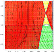
Figure 1. A contour plot of $\operatorname{Re}{\Phi_{m}(z)}$ in $E_{m}$ by Mathematica for $p=3$, $m=2$, and $u=0.5$. The region $\overline{R}_{m}$ ($\underline{R}_{m}$, respectively) is indicated by yellow (green, respectively). The region $D_{m}$ is indicated by red, which overwrites a part of $\overline{R}_{m}\cup\underline{R}_{m}$.

Before we give a proof, let us define several lines as indicated in Figure 2.

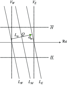
Figure 2. The region $U_{m}$ is between $L_{E}$ and $L_{W}$.

$$L_{\sigma} :\operatorname{Re}{z}-\frac{2p\pi}{u}\operatorname{Im}{z}=0,$$

$$L_{E} :\operatorname{Re}{z}+\frac{u}{2p\pi}\operatorname{Im}{z}=\frac{m+1}{p},$$

$$L_{M} :\operatorname{Re}{z}+\frac{u}{2p\pi}\operatorname{Im}{z}=\frac{2m+1}{2p},$$

$$L_{W} :\operatorname{Re}{z}+\frac{u}{2p\pi}\operatorname{Im}{z}=\frac{m}{p},$$

$$\overline{H} :\operatorname{Im}{z}=2\operatorname{Im}\sigma_{m},$$

$$\underline{H} :\operatorname{Im}{z}=-2\operatorname{Im}\sigma_{m},$$

$$V_{E} :\operatorname{Re}{z}=\frac{m+1}{p},$$

$$V_{W} :\operatorname{Re}{z}=\frac{m}{p}.$$

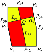
Figure 3. The region $E_{m}$.

Note that $E_{m}$ is the hexagonal region surrounded by $\overline{H}$, $L_{E}$, $V_{E}$, $\underline{H}$, $L_{W}$, and $V_{W}$. Strictly speaking, we need to push $L_{E}$ and $L_{W}$ slightly inside. We name the vertices of its boundary as indicated in Figure 3. Their coordinates are given as:

$$P_{0} :\frac{m}{p},$$

$$P_{1} :\frac{m}{p}+\frac{\overline{\xi}}{p\pi}\operatorname{Im}\sigma_{m},$$

$$P_{2} :\frac{m+1}{p}-2\operatorname{Im}\sigma_{m}\sqrt{-1},$$

$$P_{3} :\frac{m+1}{p},$$

$$P_{4} :\frac{m+1}{p}-\frac{\overline{\xi}}{p\pi}\operatorname{Im}\sigma_{m},$$

$$P_{5} :\frac{m}{p}+2\operatorname{Im}\sigma_{m}\sqrt{-1},$$

where $\overline{\xi}$ is the complex conjugate of $\xi$.

We also put $P_{12}:=L_{M}\cap\underline{H}$, $P_{34}:=L_{E}\cap L_{\sigma}$, $P_{45}:=L_{M}\cap\overline{H}$, and $P_{50}:=L_{W}\cap L_{\sigma}$. Their coordinates are given as follows.

$$P_{12} :\frac{2m+1}{2p}+\frac{\overline{\xi}}{p\pi}\operatorname{Im}\sigma_{m},$$

$$P_{34} :\frac{2(m+1)\pi\sqrt{-1}}{\xi},$$

$$P_{45} :\frac{2m+1}{2p}-\frac{\overline{\xi}}{p\pi}\operatorname{Im}\sigma_{m},$$

$$P_{50} :\frac{m\overline{\xi}\sqrt{-1}}{2p^{2}\pi}.$$

We use the following lemmas in the proof of Proposition 5.1 below.

Lemma 5.2.

We have the inequalities $0<\operatorname{Re}{F(0)}<\operatorname{Re}{F(\sigma_{0})}$.

Lemma 5.3.

We have the inequality $\operatorname{Re}{\Phi_{m}\left(P_{12}\right)}<\operatorname{Re}{\Phi_{m}(\sigma_{m})}$.

Proofs of the lemmas are given in Section 8.

Proof of Proposition 5.1.

In the following proof, we assume that $\nu$ is sufficiently small. We may need to modify the argument below slightly if necessary.

(1). We know that $\Phi_{m}(z)$ is of the form (4.6). Since $a_{2}=\frac{1}{2}\xi\sqrt{-1}\sqrt{(2\cosh{u}+1)(3-2\cosh{u})}$ and $0<u<\operatorname{arccosh}(3/2)$, we see that $\operatorname{Re}{a_{2}}=-p\pi\sqrt{(2\cosh{u}+1)(3-2\cosh{u})}<0$. So we conclude that $\Phi_{m}(z)$ is of this form.

(2). Writing $z=x+y\sqrt{-1}$, we have

$$\frac{\partial}{\partial\,y}\operatorname{Re}{\Phi_{m}(x+y\sqrt{-1})}=-\arg\tau(x,y)$$

from (4.2), where we put $\tau(x,y):=2\cosh(u)-2\cosh\bigl{(}\xi(x+y\sqrt{-1})\bigr{)}$. Since we have

$$\operatorname{Im}\tau(x,y)=-2\sinh(ux-2p\pi y)\sin(uy+2p\pi x),$$

we see that $\operatorname{Im}\tau(x,y)>0$ ($\operatorname{Im}\tau(x,y)<0$, respectively) if and only if $ux<2p\pi y$ and $2k\pi<uy+2p\pi x<(2k+1)\pi$ for some integer $k$, or $ux>2p\pi y$ and $(2l-1)\pi<uy+2p\pi x<2l\pi$ for some integer $l$ ($ux>2p\pi y$ and $2k\pi<uy+2p\pi x<(2k+1)\pi$ for some integer $k$, or $ux<2p\pi y$ and $(2l-1)\pi<uy+2p\pi x<2l\pi$ for some integer $l$, respectively). Since $z\in U_{m}$, we have $2m\pi<uy+2p\pi x<2(m+1)\pi$. So we have

$$\frac{\partial}{\partial\,y}\operatorname{Re}{\Phi_{m}(x+y\sqrt{-1})}>0\quad\text{if and only if}$$

$$ux>2p\pi y 2m\pi<uy+2p\pi x<(2m+1)\pi$$ and

$$\quad\text{or $ux<2p\pi y$ and $(2m+1)\pi<uy+2p\pi x<2(m+1)\pi$},$$

and

$$\frac{\partial}{\partial\,y}\operatorname{Re}{\Phi_{m}(x+y\sqrt{-1})}<0\quad\text{if and only if}$$

$$ux<2p\pi y 2m\pi<uy+2p\pi x<(2m+1)\pi$$ and

$$\quad\text{or $ux>2p\pi y$ and $(2m+1)\pi<uy+2p\pi x<2(m+1)\pi$}.$$

Therefore, fixing $x$, $\operatorname{Re}{\Phi_{m}(x+y\sqrt{-1})}$ is monotonically increasing (decreasing, respectively) with respect to $y$ in the red region (yellow region, respectively) in Figure 3.

Next, we will show (i) the segment $\overline{P_{50}P_{34}}\subset L_{\sigma}$ except $\sigma_{m}$, (ii) the segment $\overline{P_{3}P_{34}}\subset L_{E}$, and (iii) the segment $\overline{P_{12}P_{45}}\subset L_{M}$ are in $D_{m}$. See Figure 4

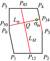
Figure 4. The red segments are in $D_{m}$.

(i): Consider the segment of $L_{\sigma}$ between $L_{W}$ and $L_{E}$ that is parametrized as $\ell_{\sigma}(t):=t\sigma_{m}$ ($\frac{2m\pi}{2(m+1)\pi+\theta}\leq t\leq\frac{2(m+1)\pi}{2(m+1)\pi+\theta}$). Then we have

$$\frac{d}{d\,t}\operatorname{Re}\Phi_{m}\left(\ell_{\sigma}(t)\right) =\operatorname{Re}\left(\sigma_{m}\log\bigl{(}2\cosh(u)-2\cosh(t\sigma_{m}\xi\bigr{)}\right)$$

$$=(\operatorname{Re}\sigma_{m})\log\left(2\cosh(u)-2\cos\left(\bigl{(}\theta+2(m+1)\pi\bigr{)}t\right)\right).$$

Since $2m\pi\leq\bigl{(}2(m+1)\pi+\theta\bigr{)}t\leq 2(m+1)\pi$ and $\cosh{u}-1/2=\cosh\varphi(u)=\cos\theta$, we see that $\frac{d}{d\,t}\operatorname{Re}\Phi_{m}\left(\ell_{\sigma}(t)\right)>0$ if and only if $\frac{2m\pi-\theta}{2(m+1)\pi+\theta}<t<1$, and that $\frac{d}{d\,t}\operatorname{Re}\Phi_{m}\left(\ell_{\sigma}(t)\right)<0$ if and only if $\frac{2m\pi}{2(m+1)\pi+\theta}<t<\frac{2m\pi-\theta}{2(m+1)\pi+\theta}$ or $1<t<\frac{2(m+1)\pi}{2(m+1)\pi+\theta}$.

Let $P_{W}$ be the point $L_{\sigma}\cap L_{W}$ with coordinate $\frac{2m\pi\sqrt{-1}}{\xi}$. Since $\Phi_{m}(P_{W})=F(0)$ and $\Phi_{m}(\sigma_{m})=F(\sigma_{0})$, Lemma 5.2 implies that $\operatorname{Re}\Phi_{m}\left(\ell_{\sigma}(t)\right)$ takes its maximum $\operatorname{Re}\Phi_{m}(\sigma_{m})$ at $t=1$. This shows that $L_{\sigma}\cap E_{m}$ is in $D_{m}$ except for $\sigma_{m}$.

(ii): Consider the segment $\overline{P_{3}P_{4}}$ that is parametrized as $\ell_{E}(t):=\frac{m+1}{p}-\frac{u}{2p\pi}t+t\sqrt{-1}=\frac{m+1}{p}-\frac{\overline{\xi}}{2p\pi}t$ ($0\leq t\leq 2\operatorname{Im}\sigma_{m}$). We have

$$\frac{d}{d\,t}\operatorname{Re}{\Phi_{m}\left(\ell_{E}(t)\right)}$$

$$= -\operatorname{Re}\left(\frac{\overline{\xi}}{2p\pi}\log\left(2\cosh{u}-2\cosh\left(\xi\ell_{E}(t)\right)\right)\right)$$

$$= -\frac{u}{2p\pi}\log\left(2\cosh{u}-2\cosh\left(\frac{(m+1)u}{p}-\frac{|\xi|^{2}t}{2p\pi}\right)\right)>0,$$

because

$$\left|\frac{(m+1)u}{p}-\frac{|\xi|^{2}t}{2p\pi}\right|$$

$$\leq \max\left\{\frac{(m+1)u}{p},\left|\frac{(m+1)u}{p}-\frac{u\bigl{(}\theta+2(m+1)\pi\bigr{)}}{p\pi}\right|\right\}$$

$$= \max\left\{\frac{(m+1)u}{p},\frac{(m+1)u}{p}+\frac{u\theta}{p\pi}\right\}=\frac{(m+1)u}{p}\leq u.$$

Since the point $P_{34}$ is in $D_{m}$, we conclude that $\overline{P_{3}P_{34}}\subset D_{m}$.

(iii): The line $L_{M}$ between $\underline{H}$ and $\overline{H}$ is parametrized as $\ell_{M}(t):=\frac{2m+1}{2p}-\frac{u}{2p\pi}t+t\sqrt{-1}=\frac{2m+1}{2p}-\frac{\overline{\xi}}{2p\pi}t$ ($-2\operatorname{Im}\sigma_{m}\leq t\leq 2\operatorname{Im}\sigma_{m}$). Now we have

$$\frac{d}{d\,t}\operatorname{Re}{\Phi_{m}\left(\ell_{M}(t)\right)}$$

$$= -\operatorname{Re}\left(\frac{\overline{\xi}}{2p\pi}\log\left(2\cosh(u)-2\cosh\left(\frac{(2m+1)}{2p}\xi-\frac{|\xi|^{2}}{2p\pi}t\right)\right)\right)$$

$$= -\frac{u}{2p\pi}\log\left(2\cosh(u)+2\cosh\left(\frac{(2m+1)u}{2p}-\frac{|\xi|^{2}}{2p\pi}t\right)\right)<0.$$

Since $\ell_{M}(-2\operatorname{Im}\sigma_{m})=P_{12}$, from Lemma 5.3, we see that $\operatorname{Re}{\Phi_{m}(P_{12})}<\operatorname{Re}{\Phi_{m}(\sigma_{m})}$. Therefore every point $z$ on $\overline{P_{12}P_{45}}$ satisfies $\operatorname{Re}{\Phi_{m}(z)}<\operatorname{Re}{\Phi_{m}(\sigma_{m})}$.

Now we split $E_{m}$ into five pieces:

$$E_{m,1} :=\{z\in E\mid b_{m}^{-}\leq\operatorname{Re}{z}\leq\operatorname{Re}{P_{45}}\},$$

$$E_{m,2} :=\{z\in E\mid\operatorname{Re}{P_{45}\leq\operatorname{Re}{z}}\leq\operatorname{Re}{Q}\},$$

$$E_{m,3} :=\{z\in E\mid\operatorname{Re}{Q}\leq\operatorname{Re}{z}\leq\operatorname{Re}{P_{12}}\},$$

$$E_{m,4} :=\{z\in E\mid\operatorname{Re}{P_{12}}\leq\operatorname{Re}{z}\leq\operatorname{Re}{\sigma_{m}}\},$$

$$E_{m,5} :=\{z\in E\mid\operatorname{Re}{\sigma_{m}}\leq\operatorname{Re}{z}\leq\operatorname{Re}{P_{34}}\},$$

$$E_{m,6} :=\{z\in E\mid\operatorname{Re}{P_{34}}\leq\operatorname{Re}{z}\leq b_{m}^{+}\},$$

where $Q$ is the intersection of $L_{M}$ and $L_{\sigma}$. See Figure 5.

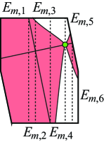
Figure 5. The red region is $D_{m}$.

Note the following:

• $\operatorname{Re}{P_{1}}<\operatorname{Re}{P_{45}}$: This is because $\operatorname{Re}{P_{1}}-\operatorname{Re}{P_{45}}=-\frac{1}{2p}+2\frac{u}{p\pi}\operatorname{Im}\sigma_{m}$, which can be proved to be negative.

• $\operatorname{Re}{P_{12}}<\operatorname{Re}{P_{4}}$: This is because $\operatorname{Re}{P_{12}}-\operatorname{Re}{P_{4}}=-\frac{1}{2p}+2\frac{u}{p\pi}\operatorname{Im}\sigma_{m}<0$ as above.

• $\operatorname{Re}{P_{12}}<\operatorname{Re}{\sigma_{m}}$: This is because $\operatorname{Re}{P_{12}}-\operatorname{Re}\sigma_{m}=\frac{2m+1}{2p}+\frac{u}{p\pi}\operatorname{Im}\sigma_{m}-\operatorname{Re}\sigma_{m}<0$.

• $\operatorname{Re}{\sigma_{m}}$ can be greater than, less than, or equal to $\operatorname{Re}{P_{4}}$.

In the following, we will show that any point in $\left(E_{m,1}\cup E_{m,2}\cup E_{m,3}\cup E_{m,4}\right)\cap D_{m}$ can be connected to a point on $L_{\sigma}$ by a segment contained in $D_{m}$, and that any point in $\left(E_{m,5}\cup E_{m,6}\right)\cap D_{m}$ can also be connected to a point on $L_{\sigma}$ by a segment contained in $D_{m}$. We will also show that the vertical line through $\sigma_{m}$ does not intersect with $D_{m}$. Then, we conclude that $D_{m}\cap E_{m}$ has two connected components $\left(E_{m,1}\cup E_{m,2}\cup E_{m,3}\cup E_{m,4}\right)\cap D_{m}$ and $\left(E_{m,5}\cup E_{m,6}\right)\cap D_{m}$ because $L_{\sigma}\setminus\{\sigma_{m}\}$ has two connected components.

• $E_{m,1}$: Since $\operatorname{Re}{\Phi_{m}(x+y\sqrt{-1})}<\operatorname{Re}{\Phi_{m}(\sigma_{m})}$ when $x+y\sqrt{-1}$ is on $L_{\sigma}$ and $\operatorname{Re}{\Phi_{m}(x+y\sqrt{-1})}$ decreases whether $y$ increases or decreases fixing $x\in\left[b_{m}^{-},\operatorname{Re}{P_{45}}\right]$, we conclude that $\operatorname{Re}{\Phi_{m}(x+y\sqrt{-1})}<\operatorname{Re}{\Phi_{m}(\sigma)}$ for any $x+y\sqrt{-1}\in E_{m,1}$. So we can connect any point in $E_{m,1}$ to a point on $L_{\sigma}$.

• $E_{m,2}$: Figure 6 indicates a graph of $\operatorname{Re}{\Phi_{m}(x+y\sqrt{-1})}$ for $x+y\sqrt{-1}\in E_{m,2}$ with fixed $x$.

  

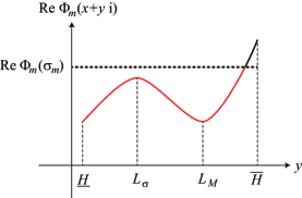
  Figure 6. The vertical axis is $\operatorname{Re}{\Phi_{m}(x+y\sqrt{-1})}$ and the horizontal axis is $y$ with fixed $x$. The red part is included in $D_{m}$. Note that the local maximum is less than $\operatorname{Re}{\Phi_{m}(\sigma_{m})}$.

  This figure shows that any point in $E_{m,2}\cap D_{m}$ can be connected to a point on $L_{\sigma}$ by a vertical segment in $D_{m}$.

• $E_{m,3}$: A graph of $\operatorname{Re}{\Phi_{m}(x+y\sqrt{-1})}$ for $x+y\sqrt{-1}\in E_{m,3}$ with fixed $x$ looks like Figure 6 because $\overline{P_{12}P_{45}}\subset D_{m}$.

  

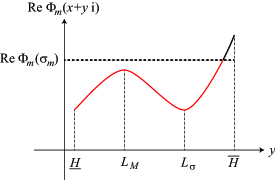
  Figure 7. The vertical axis is $\operatorname{Re}{\Phi_{m}(x+y\sqrt{-1})}$ and the horizontal axis is $y$ for fixed $x$. The red part is included in $D_{m}$.

  Therefore the argument as before shows that any point in $E_{m,3}\cap D_{m}$ can be connected to a point on $L_{\sigma}$ by a vertical segment in $D_{m}$.

• $E_{m,4}$: Starting at a point on $L_{\sigma}$, whether $y$ increases or decreases, $\operatorname{Re}\Phi_{m}(x+y\sqrt{-1})$ increases. Therefore any point in $E_{m,4}\cap D_{m}$ can be connected to a point on $L_{\sigma}$ by a vertical segment in $D_{m}$.

• $E_{m,5}$: This follows by the same reason as $E_{m,4}\cap D_{m}$.

• $E_{m,6}$: By the same argument as $E_{m,4}$, we can connect any point $z$ in $E_{m,6}\cap D_{m}$ to a point $z^{\prime}$ in $\overline{P_{3}P_{34}}$ by a vertical segment in $D_{m}$, and then connect $z^{\prime}$ to a point in $L_{\sigma}$ by a segment in $\overline{P_{3}P_{34}}$. (Precisely speaking, we need to push these segments in $E_{m,6}$.)

The fact that the vertical segment through $\sigma_{m}$ does not intersect with $D_{m}$ easily follows because $\sigma_{m}\not\in D_{m}$, and $\frac{\partial}{\partial\,y}\operatorname{Re}{\Phi_{m}(x+y\sqrt{-1})}$ is increasing (decreasing, respectively) if $x+y\sqrt{-1}$ is above $\sigma_{m}$ (below $\sigma_{m}$, respectively).

See Figure 5.

(3). From the definition, we know that $b_{m}^{-}\in E_{m,1}$ and $b_{m}^{+}\in E_{m,6}$. Therefore we can choose $\varepsilon_{m}$ such that $\operatorname{Re}{\Phi_{m}(b_{m}^{\pm})}<\operatorname{Re}{\Phi_{m}(\sigma_{m})}-\varepsilon_{m}$.

(4). Since any point $z$ ($z\neq\sigma_{m}$) on the polygonal chain $\overline{P_{0}P_{50}P_{34}}P_{3}$ satisfies $\operatorname{Re}{\Phi_{m}(z)}<\operatorname{Re}{\Phi_{m}(\sigma_{m})}$, and $\operatorname{Im}\sigma_{m}>0$, we conclude that this is in $\overline{R}_{m}$. Therefore we can connect $b_{m}^{-}$ and $b_{m}^{+}$ in $\overline{R}_{m}$.

(5). We know that if $z$ is on the polygonal chain $\overline{P_{0}P_{1}P_{12}}$, then $\operatorname{Re}{\Phi_{m}(z)}<\operatorname{Re}{\Phi_{m}(\sigma_{m})}$, which shows that $\overline{P_{0}P_{1}P_{12}}$ is in $\underline{R}_{m}$.

We will show that the segment $\overline{P_{12}P_{2}}$ is also in $\underline{R}_{m}$. From the proof of (2), we have $0>\frac{\partial}{\partial\,y}\operatorname{Re}{\Phi_{m}(x+y\sqrt{-1})}>-\pi$ if $x+y\sqrt{-1}\in\overline{P_{12}P_{2}}$. We know that if $x+y\sqrt{-1}$ is on the polygonal chain $\overline{QP_{34}P_{3}}$, then $\operatorname{Re}{\Phi_{m}(x+y\sqrt{-1})}\leq\operatorname{Re}{\Phi_{m}(\sigma_{m})}$. Since the difference of the imaginary part of $x-2\operatorname{Im}\sigma_{m}\sqrt{-1}$ and $x+y\sqrt{-1}$ is less than $4\operatorname{Im}\sigma_{m}$ if $x+y\sqrt{-1}$ is on the polygonal chain $\overline{QP_{34}P_{3}}$, we have $\operatorname{Re}{\Phi_{m}(x-2\operatorname{Im}\sigma_{m}\sqrt{-1})}-\operatorname{Re}{\Phi_{m}(x+y\sqrt{-1})}<4\pi\operatorname{Im}\sigma_{m}$. Therefore $\operatorname{Re}{\Phi_{m}(x-2\operatorname{Im}\sigma_{m}\sqrt{-1})}-\operatorname{Re}{\Phi_{m}(\sigma_{m})}<2\pi\times 2\operatorname{Im}\sigma_{m}$, proving that $z\in\underline{R}_{m}$ if $z$ is on $\overline{P_{12}P_{2}}$.

The segment $\overline{P_{2}P_{3}}$ is also in $\underline{R}_{m}$. This is because $\frac{\partial}{\partial\,y}\bigl{(}\operatorname{Re}{\Phi_{m}\bigl{(}(m+1)/p+y\sqrt{-1}\bigr{)}}+2\pi y\bigr{)}=\frac{\partial}{\partial\,y}\operatorname{Re}{\Phi_{m}\bigl{(}(m+1)/p+y\sqrt{-1}\bigr{)}}+2\pi>0$ and $P_{3}\in\underline{R}_{m}$.

Now, we can connect $b_{m}^{-}$ and $b_{m}^{+}$ by the polygonal chain $\overline{P_{0}P_{1}P_{2}P_{3}}$.

The proof is complete. ∎

6. Proof of Theorem 1.4

Now we can prove Theorem 1.4

Proof of Theorem 1.4.

Since $f_{N}(z)$ uniformly converges to $F(z)$ in the region (4.1), $f_{N}\left(z-\frac{2m\pi\sqrt{-1}}{\xi}\right)$ uniformly converges to $\Phi_{m}(z)$ in (5.1). So we can use [31, Proposition 4.2] (see also Remark 4.4 there) to conclude that

(6.1) $$\frac{1}{N}\sum_{m/p+\nu/p\leq k/N\leq(m+1)/p-\nu/p}\exp\left(N\times f_{N}\left(\frac{2k+1}{2N}-\frac{2m\pi\sqrt{-1}}{\xi}\right)\right)$$

$$= \int_{m/p+\nu/p}^{(m+1)/p-\nu/p}e^{N\Phi_{m}(z)}\,dz+O(e^{-N\varepsilon^{\prime}_{m}})$$

for some $\varepsilon^{\prime}_{m}>0$ from Proposition 5.1.

Since $\Phi_{m}(z)$ is of the form (4.6) in $E_{m}$, we can apply the saddle point method (see [31, Proposition 3.2 and Remark 3.3]) to obtain

(6.2) $$\int_{m/p+\nu/p}^{(m+1)/p-\nu/p}e^{N\Phi_{m}(z)}\,dz=\frac{\sqrt{\pi}e^{N\times F(\sigma_{0})}}{\sqrt{-\frac{1}{2}\xi\sqrt{(2\cosh{u}+1)(2\cosh{u}-3)}}\sqrt{N}}\bigl{(}1+O(N^{-1})\bigr{)},$$

where we choose the sign of the outer square root so that its real part is positive (recall that we choose the sign the inner square root so that it is a positive multiple of $\sqrt{-1}$). From (6.1) and (6.2), we have

(6.3) $$\sum_{m/p+\nu/p\leq k/N\leq(m+1)/p-\nu/p}\exp\left(N\times f_{N}\left(\frac{2k+1}{2N}-\frac{2m\pi\sqrt{-1}}{\xi}\right)\right)$$

$$= \frac{\sqrt{2\pi}e^{\pi\sqrt{-1}/4}}{\bigl{(}(1+2\cosh{u})(3-2\cosh{u})\bigr{)}^{1/4}}e^{N\times F(\sigma_{0})}\times\sqrt{\frac{N}{\xi}}\bigl{(}1+O(N^{-1})\bigr{)},$$

since $\operatorname{Re}{F(\sigma_{0})}>0$ from Lemma 5.2.

Now, we use the following lemma, a proof of which is given in Section 8.

Lemma 6.1.

There exists $\varepsilon>0$ such that $\operatorname{Re}{\Phi_{m}\left(\frac{m+1}{p}\right)}<\operatorname{Re}{\Phi_{m}(\sigma_{m})}-2\varepsilon$ for $m=0,1,2,\dots,p-1$. Moreover there exists $\tilde{\delta}_{m}>0$ such that if $\frac{m}{p}\leq\frac{k}{N}<\frac{m}{p}+\tilde{\delta}_{m}$ or $\frac{m+1}{p}-\tilde{\delta}_{m}<\frac{k}{N}<\frac{m+1}{p}$, then we have

(6.4) $$\operatorname{Re}{f_{N}\left(\frac{2k+1}{2N}-\frac{2m\pi\sqrt{-1}}{\xi}\right)}<\operatorname{Re}{F(\sigma_{0})}-\varepsilon$$

for sufficiently large $N$.

If we choose $\nu$ so that $\nu/p\leq\tilde{\delta}_{m}$, the sums

$$\sum_{m/p\leq k/N<m/p+\nu/p}\exp\left(N\times f_{N}\left(\frac{2k+1}{2N}-\frac{2m\pi\sqrt{-1}}{\xi}\right)\right)$$

and

$$\sum_{(m+1)/p-\nu/p<k/N\leq(m+1)/p}\exp\left(N\times f_{N}\left(\frac{2k+1}{2N}-\frac{2m\pi\sqrt{-1}}{\xi}\right)\right)$$

are both of order $O\left(Ne^{N(\operatorname{Re}{F(\sigma_{0})}-\varepsilon)}\right)$ from Lemma 6.1. Therefore we have

$$\sum_{m/p\leq k/N\leq(m+1)/p}\exp\left(N\times f_{N}\left(\frac{2k+1}{2N}-\frac{2m\pi\sqrt{-1}}{\xi}\right)\right)$$

$$= \sum_{m/p+\nu/p\leq k/N\leq(m+1)/p-\nu/p}\exp\left(N\times f_{N}\left(\frac{2k+1}{2N}-\frac{2m\pi\sqrt{-1}}{\xi}\right)\right)$$

$$+O\left(Ne^{N(\operatorname{Re}{F(\sigma_{0})}-\varepsilon)}\right)$$

$$= \frac{\sqrt{2\pi}e^{\pi\sqrt{-1}/4}}{\bigl{(}(1+2\cosh{u})(3-2\cosh{u})\bigr{)}^{1/4}}e^{N\times F(\sigma_{0})}\times\sqrt{\frac{N}{\xi}}\bigl{(}1+O(N^{-1})\bigr{)}$$

where the second equality follows from (6.3).

It follows that

$$J_{N}\left(E;e^{\xi/N}\right) =\frac{1}{2\sinh(u/2)}\left(\sum_{m=0}^{p-1}\beta_{p,m}\right)\times\frac{\sqrt{2\pi}e^{\pi\sqrt{-1}/4}}{\bigl{(}(1+2\cosh{u})(3-2\cosh{u})\bigr{)}^{1/4}}$$

$$\quad\times\sqrt{\frac{N}{\xi}}e^{N\times F(\sigma_{0})}\bigl{(}1+O(N^{-1})\bigr{)}$$

from (3.2). Using (2.1) with $N=p$ and $q=e^{4N\pi^{2}/\xi}$, we have

$$\sum_{m=0}^{p-1}\beta_{m,p}=J_{p}\left(E;e^{4N\pi^{2}/\xi}\right).$$

Therefore we have

$$J_{N}\left(E;e^{\xi/N}\right)= \frac{1}{2\sinh(u/2)}J_{p}\left(E;e^{4N\pi^{2}/\xi}\right)\times\frac{\sqrt{2\pi}e^{\pi\sqrt{-1}/4}}{\bigl{(}(1+2\cosh{u})(3-2\cosh{u})\bigr{)}^{1/4}}$$

$$\quad\times\sqrt{\frac{N}{\xi}}e^{N\times F(\sigma_{0})}\bigl{(}1+O(N^{-1})\bigr{)}.$$

Putting

$$S_{E}(u) :=\xi\bigl{(}F(\sigma_{0})+2\pi\sqrt{-1}\bigr{)}$$

$$=\operatorname{Li}_{2}\left(e^{-u-\varphi(u)}\right)-\operatorname{Li}_{2}\left(e^{-u+\varphi(u)}\right)+u\bigl{(}\varphi(u)+2\pi\sqrt{-1}\bigr{)},$$

$$T_{E}(u) :=\frac{2}{\sqrt{(2\cosh{u}+1)(2\cosh{u}-3)}},$$

we finally have

$$J_{N}\left(E;e^{\xi/N}\right)\\ =\frac{\sqrt{-\pi}}{2\sinh(u/2)}T_{E}(u)^{1/2}J_{p}\left(E;e^{4N\pi^{2}/\xi}\right)\left(\frac{N}{\xi}\right)^{1/2}e^{\frac{N}{\xi}\times S_{E}(u)}\bigl{(}1+O(N^{-1})\bigr{)},$$

which proves Theorem 1.4. ∎

We can see that the cohomological adjoint Reidemeister torsion $T_{E}(u)$ equals $\pm T_{E}(u)$ and the Chern–Simons invariant $\operatorname{CS}_{u,v(u)}(\rho)$ is given by $S_{E}(u)-u\pi\sqrt{-1}-\frac{1}{4}uv(u)\pmod{\pi^{2}\mathbb{Z}}$. See for example [29, Chapter 5] for calculation of the adjoint Reidemeister torsion and the Chern–Simons invariant.

7. Quantum modularity

For $\eta:=\begin{pmatrix}a&b\\ c&d\end{pmatrix}\in\mathrm{SL}(2;\mathbb{Z})$ and a complex number $z$, define $\eta(z):=\dfrac{az+b}{cz+d}$ as usual. We also define $\hbar_{\eta}(z):=\frac{2\pi\sqrt{-1}}{z-\eta^{-1}(\infty)}=\frac{2c\pi\sqrt{-1}}{cz+d}$.

In [36], D. Zagier conjectured the following.

Conjecture 7.1 (Quantum modularity conjecture).

Let $K$ be a hyperbolic knot in $S^{3}$ and $\eta:=\begin{pmatrix}a&b\\ c&d\end{pmatrix}\in\mathrm{SL}(2;\mathbb{Z})$ with $c>0$. Putting $X_{0}:=N/p$ for positive integers $N$ and $p$, the following asymptotic equivalence holds.

(7.1) $$\frac{J_{cN+dp}\left(K;e^{2\pi\sqrt{-1}\eta(X_{0})}\right)}{J_{p}\left(K;e^{2\pi\sqrt{-1}X_{0}}\right)}\\ \underset{N\to\infty}{\sim}C_{K,\eta}\left(\frac{2\pi}{\hbar_{\eta}(X_{0})}\right)^{3/2}\exp\left(\frac{\sqrt{-1}\operatorname{CV}(K)}{\hbar_{\eta}(X_{0})}\right),$$

where $C_{K,\eta}$ is a complex number depending only on $\eta$ and $K$.

Note that Conjecture 7.1 is just a part of Zagier’s original quantum modularity conjecture. See [36, 7, 1] for more details.

Remark 7.2.

The modularity conjecture was proved by S. Garoufalidis and D. Zagier [7] in the case of the figure-eight knot, and by S. Bettin and S. Drappeau [1] for hyperbolic knots with at most seven crossings except for $7_{2}$.

Bettin and Drappeau also proved that for the figure-eight knot $E$, $C_{E,\eta}$ is given as follows.

$$C_{E,\eta}=\frac{ce^{3\pi\sqrt{-1}/4}}{3^{1/4}}\prod_{g=1}^{c}|\omega_{g}|^{2g/c}\left(\sum_{r=1}^{c}\prod_{g=1}^{r}|\omega_{g}|^{2}\right),$$

where $\omega_{g}:=1-\exp\left(2\pi\sqrt{-1}(\frac{ag}{c}-\frac{5}{6c})\right)$.

Since

$$S_{E}(0)=\operatorname{Li}_{2}\left(e^{\pi\sqrt{-1}/3}\right)-\operatorname{Li}_{2}\left(e^{-\pi\sqrt{-1}/3}\right)=\operatorname{Vol}\left(S^{3}\setminus{E}\right)\sqrt{-1}$$

(see, for example, [22, Appendix]), if $K$ is the figure-eight knot $E$ and $\eta=\begin{pmatrix}0&-1\\ 1&0\end{pmatrix}$, (7.1) turns out to be

(7.2) $$\frac{J_{N}\left(E;e^{2p\pi/N}\right)}{J_{p}\left(E;e^{2N\pi\sqrt{-1}/p}\right)}\\ \underset{N\to\infty}{\sim}-2\pi^{3/2}T_{E}(0)^{1/2}\left(\frac{N}{2p\pi\sqrt{-1}}\right)^{3/2}\exp\left(\frac{NS_{E}(0)}{2p\pi\sqrt{-1}}\right).$$

Here we use the fact that $E$ is amphicheiral, that is, $E$ is equivalent to its mirror image, to conclude $J_{N}(E;q)=J_{N}(E;q^{-1})$. Compare (7.2) with (1.2), noting that $\xi=2p\pi\sqrt{-1}$ when $u=0$.

We can regard (1.2) as a kind of quantum modularity with $\eta=\begin{pmatrix}0&-1\\ 1&0\end{pmatrix}$ as follows.

Put $X:=\frac{2N\pi\sqrt{-1}}{\xi}$. Note that $\operatorname{Re}{X}\to\infty$ as $N\to\infty$. We have $\eta(X)=\frac{-\xi}{2N\pi\sqrt{-1}}$, $\exp(2\pi\sqrt{-1}X)=e^{-4N\pi^{2}/\xi}$, $\exp\bigl{(}2\pi\sqrt{-1}\eta(X)\bigr{)}=e^{-\xi/N}$, and $\hbar_{\eta}(X)=\xi/N$. Since the figure-eight knot is amphicheiral, (1.2) can be written as

$$\frac{J_{N}\left(E;e^{2\pi\sqrt{-1}\eta(X)}\right)}{J_{p}\left(E;e^{2\pi\sqrt{-1}X}\right)}\sim\frac{\sqrt{-\pi}}{2\sinh(u/2)}\left(\frac{T_{E}(u)}{\hbar_{\eta}(X)}\right)^{1/2}\exp\left(\frac{S_{E}(u)}{\hbar_{\eta}(X)}\right).$$

We would like to generalize this to other elements of $\mathrm{SL}(2;\mathbb{Z})$ and other hyperbolic knots in $S^{3}$. Some computer experiments indicate the following conjecture stated in Introduction.

Conjecture 7.3 (Quantum modularity conjecture for the colored Jones polynomial).

Let $K\subset S^{3}$ be a hyperbolic knot, and $u$ a small complex number that is not a rational multiple of $\pi\sqrt{-1}$. For positive integers $p$ and $N$, put $\xi:=u+2p\pi\sqrt{-1}$ and $X:=\frac{2N\pi\sqrt{-1}}{\xi}$. Then for any $\eta=\begin{pmatrix}a&b\\ c&d\end{pmatrix}\in\mathrm{SL}(2;\mathbb{Z})$ with $c>0$, the following asymptotic equivalence holds.

(7.3) $$\frac{J_{cN+dp}\left(K;e^{2\pi\sqrt{-1}\eta(X)}\right)}{J_{p}\left(K;e^{2\pi\sqrt{-1}X}\right)}\underset{N\to\infty}{\sim}C_{K,\eta}(u)\frac{\sqrt{-\pi}}{2\sinh(u/2)}\left(\frac{T_{K}(u)}{\hbar_{\eta}(X)}\right)^{1/2}\exp\left(\frac{S_{K}(u)}{\hbar_{\eta}(X)}\right),$$

where $C_{K,\eta}(u)\in\mathbb{C}$ does not depend on $p$.

Note that $cN+dp$ comes from the denominator of $\eta(N/p)=\eta\left(X\bigm{|}_{u=0}\right)$.

Remark 7.4.

Compare the exponent $1/2$ of $1/\hbar_{\eta}(X)=\frac{cX+d}{2c\pi\sqrt{-1}}$ in (7.3) with $3/2$ in (7.1). Our modularity would have weight $1/2$ rather than $3/2$.

Remark 7.5.

Since $(-\eta)(X)=\eta(X)$, we may assume that $c\geq 0$.

If $c=0$, then $\eta=\pm\begin{pmatrix}1&k\\ 0&1\end{pmatrix}$ for some integer $k$. Since $\eta(X)=X+k$, we have $\exp\bigl{(}2\pi\sqrt{-1}\eta(X)\bigr{)}=\exp(2\pi\sqrt{-1}X)$ and so $J_{p}\left(E;e^{2\pi\sqrt{-1}\eta(X)}\right)=J_{p}\left(E;e^{2\pi\sqrt{-1}X}\right)$.

Remark 7.6.

When $p=1$ and $\eta=\begin{pmatrix}0&-1\\ 1&0\end{pmatrix}$, (7.3) becomes

$$J_{N}\left(K;e^{-(u+2\pi\sqrt{-1})/N}\right)\\ \underset{N\to\infty}{\sim}C_{K,\eta}(u)\frac{\sqrt{-\pi}}{2\sinh(u/2)}\left(T_{K}(u)\right)^{1/2}\left(\frac{N}{u+2\pi\sqrt{-1}}\right)^{1/2}\exp\left(\frac{N\times S_{K}(u)}{u+2\pi\sqrt{-1}}\right),$$

which coincides with [24, Conjecture 1.6] with $C_{K,\eta}(u)=1$. See also [2, 9]. Strictly speaking, we need to take the mirror image $\overline{K}$ of $K$ because $J_{N}\left(\overline{K};e^{-(u+2\pi\sqrt{-1})/N}\right)=J_{N}\left(K;e^{(u+2\pi\sqrt{-1})/N}\right)$.

8. Lemmas

In this section we prove lemmas that we use.

Proof of Lemma 2.1.

Recall that $\xi=u+2p\pi\sqrt{-1}$ and $\gamma=\frac{\xi}{2N\pi\sqrt{-1}}$.

Since $\operatorname{Re}{\gamma}=p/N>0$, $\sinh(\gamma x)\underset{N\to\infty}{\sim}\frac{e^{\xi x}}{2}$ and $\sinh(\gamma x)\underset{N\to-\infty}{\sim}\frac{-e^{-\xi x}}{2}$. So we have

$$\frac{e^{(2z-1)x}}{x\sinh(x)\sinh(\gamma x)} \underset{N\to\infty}{\sim}\frac{1}{2x}e^{(2z-\gamma-2)x},$$

and

$$\frac{e^{(2z-1)x}}{x\sinh(x)\sinh(\gamma x)} \underset{N\to-\infty}{\sim}\frac{-1}{2x}e^{(2z+\gamma)x}.$$

Therefore if $-\operatorname{Re}\gamma/2<\operatorname{Re}{z}<1+\operatorname{Re}\gamma/2$, then the integral converges, completing the lemma. ∎

The following proof is almost the same as [27, Proposition 2.8]. See also [31, Proposition A.1].

Proof of Lemma 2.4.

We will show that $T_{N}(z)=\frac{N}{\xi}\mathcal{L}_{2}(z)+O(1/N)$.

Recalling that $\xi=2N\pi\gamma\sqrt{-1}$, we have

$$\left|T_{N}(z)-\frac{N}{\xi}\mathcal{L}_{2}(z)\right| =\frac{1}{4}\int_{\mathrel{\mathop{\mathbb{R}}\limits^{\vbox to0.0pt{\kern-1.0pt\hbox{$\scriptstyle\frown$}\vss}}}}\left|\frac{e^{(2z-1)x}}{\gamma x^{2}\sinh(x)}\left(\frac{\gamma x}{\sinh(\gamma x)}-1\right)\right|\,dx$$

$$\leq\frac{N\pi}{2|\xi|}\int_{\mathrel{\mathop{\mathbb{R}}\limits^{\vbox to0.0pt{\kern-1.0pt\hbox{$\scriptstyle\frown$}\vss}}}}\left|\frac{e^{(2z-1)x}}{x^{2}\sinh(x)}\left(\frac{\gamma x}{\sinh(\gamma x)}-1\right)\right|\,dx.$$

Since the Taylor expansion of $\frac{\sinh(y)}{y}$ around $y=0$ is $1+\frac{y^{2}}{6}+\cdots$, we have $\frac{y}{\sinh(y)}=1-\frac{y^{2}}{6}+o(y^{2})$ as $y\to 0$. Therefore, we have $\left|\frac{\gamma x}{\sinh(\gamma x)}-1\right|\leq\frac{c|x|^{2}}{N^{2}}$ for some constant $c>0$ and so

$$\left|T_{N}(z)-\frac{N}{\xi}\mathcal{L}_{2}(z)\right|<\frac{c^{\prime}}{N}\int_{\mathrel{\mathop{\mathbb{R}}\limits^{\vbox to0.0pt{\kern-1.0pt\hbox{$\scriptstyle\frown$}\vss}}}}\left|\frac{e^{(2z-1)x}}{\sinh(x)}\right|\,dx,$$

where we put $c^{\prime}:=\frac{c\pi}{2|\xi|}$.

We put

$$I_{+} :=\int_{1}^{\infty}\left|\frac{e^{(2z-1)x}}{\sinh(x)}\right|\,dx,$$

$$I_{-} :=\int_{-\infty}^{-1}\left|\frac{e^{(2z-1)x}}{\sinh(x)}\right|\,dx,$$

$$I_{0} :=\int_{|x|=1,\operatorname{Im}{x}\geq 0}\left|\frac{e^{(2z-1)x}}{\sinh(x)}\right|\,dx.$$

We have

$$I_{+} \leq\int_{1}^{\infty}\frac{2e^{2x\operatorname{Re}{z}-x}}{e^{x}-e^{-x}}\,dx=\int_{1}^{\infty}\frac{2e^{2x(\operatorname{Re}{z}-1)}}{1-e^{-2x}}\,dx\leq\frac{2}{1-e^{-2}}\int_{1}^{\infty}e^{-2\nu x}\,dx$$

$$=\frac{e^{-2\nu}}{\nu(1-e^{-2})},$$

where we use the assumption $\operatorname{Re}{z}\leq 1-\nu$.

Similarly, we have

$$I_{-} \leq\int_{-\infty}^{-1}\frac{2e^{2x\operatorname{Re}{z}-x}}{e^{-x}-e^{x}}\,dx=\int_{-\infty}^{-1}\frac{2e^{2x\operatorname{Re}{z}}}{1-e^{2x}}\,dx\leq\frac{2}{1-e^{-2}}\int_{-\infty}^{-1}e^{2\nu x}\,dx$$

$$=\frac{e^{-2\nu}}{\nu(1-e^{-2})},$$

where we use the assumption $\operatorname{Re}{z}\geq\nu$.

Putting $x=e^{t\sqrt{-1}}$ ($0\leq t\leq\pi$) and $L:=\max_{|x|=1,\operatorname{Im}{x}\geq 0}|\sinh(x)|$, we have

$$I_{0}=\int_{0}^{\pi}\left|\frac{e^{(2z-1)e^{t\sqrt{-1}}}}{\sinh\left(e^{t\sqrt{-1}}\right)}\right|\times\left|\sqrt{-1}e^{t\sqrt{-1}}\right|\,dt\leq\frac{1}{L}\int_{0}^{\pi}e^{(2\operatorname{Re}{z}-1)\cos{t}-2\operatorname{Im}{z}\sin{t}}\,dt,$$

which is bounded from the above because both $\operatorname{Re}{z}$ and $\operatorname{Im}{z}$ are bounded.

Therefore, we see that $I_{+}+I_{-}+I_{0}$ is bounded from above, which implies that $\left|T_{N}(z)-\frac{N}{\xi}\mathcal{L}_{2}(z)\right|=O(1/N)$. ∎

Proof of Lemma 5.2.

Since $\operatorname{Re}{F(0)}$ coincides with $\operatorname{Re}{\Phi(w_{0})}$ in [24] (see [27, Remark 1.6]), we have $\operatorname{Re}{F(0)}>0$ from [24, Lemma 3.5].

Next, we will show that $\xi\bigl{(}F(\sigma_{0})-F(0)\bigr{)}$ is purely imaginary with positive imaginary part. Then we conclude that $\operatorname{Re}\bigl{(}F(\sigma_{0})-F(0)\bigr{)}>0$, since $\xi$ is in the first quadrant.

Since $\varphi(u)$ is purely imaginary, we have $\overline{\operatorname{Li}_{2}\left(e^{-u-\varphi(u)}\right)}=\operatorname{Li}_{2}\left(e^{-u+\varphi(u)}\right)$. So we see that $\xi\bigl{(}F(\sigma_{0})-F(0)\bigr{)}=\operatorname{Li}_{2}\left(e^{-u-\varphi(u)}\right)-\operatorname{Li}_{2}\left(e^{-u+\varphi(u)}\right)+u(\theta+2\pi)\sqrt{-1}$ is purely imaginary with imaginary part $2\operatorname{Im}\operatorname{Li}_{2}\left(e^{-u-\varphi(u)}\right)+u(\theta+2\pi)$, which coincides with $\operatorname{Im}\bigl{(}\xi\Phi(w_{0})\bigr{)}+2u\pi>0$ in [24, P. 214].

This proves the lemma. ∎

Proof of Lemma 5.3.

We have

$$\xi\left(\Phi_{m}(P_{12})-\Phi_{m}(\sigma_{m})\right)$$

$$= \operatorname{Li}_{2}\left(-e^{-u-\frac{u((6m+5)\pi+2\theta)}{2p\pi}}\right)-\operatorname{Li}_{2}\left(-e^{-u+\frac{u((6m+5)\pi+2\theta)}{2p\pi}}\right)$$

$$-\operatorname{Li}_{2}\left(e^{-u-\varphi(u)}\right)+\operatorname{Li}_{2}\left(e^{-u+\varphi(u)}\right)$$

$$+\frac{(2m+1)u\xi}{2p}+\frac{u^{2}(2(m+1)\pi+\theta)}{p\pi}-u\bigl{(}2(m+1)\pi+\theta\bigr{)}\sqrt{-1}.$$

Its real part is

$$\operatorname{Li}_{2}\left(-e^{-u-q_{m}(u)}\right)-\operatorname{Li}_{2}\left(-e^{-u+q_{m}(u)}\right)+uq_{m}(u),$$

where we put $q_{m}(u):=\frac{u((6m+5)\pi+2\theta)}{2p\pi}$, and its imaginary part is

$$-2\operatorname{Im}\operatorname{Li}_{2}\left(e^{-u-\varphi(u)}\right)-u(\pi+\theta).$$

Then we have

$$\frac{|\xi|^{2}}{u}\operatorname{Re}\left(F(P_{12})-F(\sigma_{m})\right)$$

$$= \operatorname{Re}\left(\xi\bigl{(}F(P_{12})-F(\sigma_{m})\bigr{)}\right)+\frac{2p\pi}{u}\operatorname{Im}\left(\xi\bigl{(}F(P_{12})-F(\sigma_{m})\bigr{)}\right)$$

$$= \operatorname{Li}_{2}\left(-e^{-u-q_{m}(u)}\right)-\operatorname{Li}_{2}\left(-e^{-u+q_{m}(u)}\right)+uq_{m}(u)$$

$$-\frac{2p\pi}{u}\left(2\operatorname{Im}\operatorname{Li}_{2}\left(e^{-u-\varphi(u)}\right)+u(\pi+\theta)\right).$$

By using the inequality $2\operatorname{Im}\operatorname{Li}_{2}\left(e^{-u-\varphi(u)}\right)+u\theta>0$ in [24, § 7], this is less than $c_{p,m}(u)$, where we put

$$c_{p,m}(u):=\operatorname{Li}_{2}\left(-e^{-u-q_{m}(u)}\right)-\operatorname{Li}_{2}\left(-e^{-u+q_{m}(u)}\right)+uq_{m}(u)-2p\pi^{2}.$$

Now we have

$$\frac{d}{d\,u}c_{p,m}(u)=q^{\prime}_{m}(u)\log\bigl{(}2\cosh{u}+2\cosh{q_{m}(u)}\bigr{)}+\log\left(\frac{e^{q_{m}(u)}+e^{-u}}{1+e^{-u+q_{m}(u)}}\right),$$

which can be easily seen to be positive. Since $u<\kappa$, it suffices to prove $c_{p,m}(\kappa)<0$. Since $\varphi(\kappa)=0$, we have

$$c_{p,m}(\kappa)=\operatorname{Li}_{2}\left(-e^{-\kappa(1+\frac{6m+5}{2p})}\right)-\operatorname{Li}_{2}\left(-e^{-\kappa(1-\frac{6m+5}{2p})}\right)+\frac{(6m+5)\kappa^{2}}{2p}-2p\pi^{2},$$

which is increasing with respect to $m$, fixing $p$. We will prove that $c_{p,p-1}(\kappa)<0$.

We calculate

$$c_{p,p-1}(\kappa)=\operatorname{Li}_{2}\left(-e^{\kappa(\frac{1}{2p}-4)}\right)-\operatorname{Li}_{2}\left(-e^{\kappa(-\frac{1}{2p}+2)}\right)+\left(3-\frac{1}{2p}\right)\kappa^{2}-2p\pi^{2}.$$

The derivative of $c_{p,p-1}(\kappa)$ with respect to $p$ equals

$$\frac{\kappa}{2p^{2}}\log\left(3+2\cosh\left(\kappa\left(3-\frac{1}{2p}\right)\right)\right)-2\pi^{2},$$

which is less than $-2\pi^{2}+\log(6+2\cosh(3\kappa)=-18.274\ldots<0$. It follows that $c_{p,p-1}(\kappa)<c_{1,0}(\kappa)=-14.9942\ldots<0$.

This shows that $\operatorname{Re}\bigl{(}F(P_{12})-F(\sigma_{m})\bigr{)}<0$, proving the lemma. ∎

Before proving Lemma 6.1, we prepare the following lemma.

Lemma 8.1.

Put $g(x):=4\sinh\left(\frac{\xi}{2}(1+x)\right)\sinh\left(\frac{\xi}{2}(1-x)\right)$. For an integer $0\leq m\leq p$, there exists $\delta_{m}>0$ such that $|g(l/N)|<1$ if $\frac{m}{p}-\delta_{m}<\frac{l}{N}<\frac{m}{p}+\delta_{m}$.

Proof.

For an integer $0\leq m\leq p$, we can easily see that

$$g(m/p)=2\bigl{(}\cosh{u}-\cosh(mu/p)\bigr{)}.$$

So we conclude that $g(m/p)$ is monotonically decreasing with respect to $m$. Therefore we have $0=g(1)\leq g(m/p)\leq g(0)=2\bigl{(}\cosh(u)-1\bigr{)}<2\cosh(\kappa)-2=1$. So we have $0\leq g(m/p)<1$.

Therefore, there exists $\delta_{m}>0$ such that $|g(x)|<1$ if $|x-m/p|<\delta_{m}$, completing the proof. ∎

Proof of Lemma 6.1.

From (2)-(ii) of the proof of Proposition 5.1, we know that $\frac{m+1}{p}\in D_{m}$, that is, $\operatorname{Re}{\Phi_{m}\left(\frac{m+1}{p}\right)}<\operatorname{Re}{\Phi_{m}(\sigma_{m})}$. Therefore there exists $\varepsilon>0$ such that $\operatorname{Re}{\Phi_{m}\left(\frac{m+1}{p}\right)}<\operatorname{Re}{\Phi_{m}(\sigma_{m})}-2\varepsilon$ for $m=0,1,2,\dots,p-1$.

Next, we show that there exists $\tilde{\delta}_{m}>0$ such that if $\frac{m+1}{p}-\tilde{\delta}_{m}<\frac{k}{N}<\frac{m+1}{p}$, then (6.4) holds.

We can choose $\delta^{\prime}_{m}>0$ so that $\operatorname{Re}{\Phi_{m}\left(\frac{k}{N}\right)}<\operatorname{Re}{\Phi_{m}\left(\frac{m+1}{p}\right)}+\varepsilon$ if $(m+1)/p-\delta^{\prime}_{m}<k/N<(m+1)/p$. So we have $\operatorname{Re}{\Phi_{m}\left(\frac{k}{N}\right)}<\operatorname{Re}{\Phi_{m}(\sigma_{m})}-\varepsilon$. Now recall that $f_{N}(z)$ converges to $F(z)$ in the region (4.1). Since we have

$$\operatorname{Re}\left(\frac{2k+1}{2N}-\frac{2(m-1)\pi\sqrt{-1}}{\xi}\right)+\frac{u}{2p\pi}\operatorname{Im}\left(\frac{2k+1}{2N}-\frac{2m\pi\sqrt{-1}}{\xi}\right)$$

$$= \frac{2k+1}{2N}-\frac{m}{p},$$

$$\operatorname{Re}\left(\frac{2k+1}{2N}-\frac{2m\pi\sqrt{-1}}{\xi}\right)-\frac{2p\pi}{u}\operatorname{Im}\left(\frac{2k+1}{2N}-\frac{2m\pi\sqrt{-1}}{\xi}\right)$$

$$= \frac{2k+1}{2N},$$

if $\nu/p+m/p-1/(2N)\leq k/N\leq(m+1)/p-\nu/p-1/(2N)$ and $k/N\leq 2M\pi/u+1-1/(2N)$, then $f_{N}\left(\frac{2k+1}{2N}-\frac{2m\pi\sqrt{-1}}{\xi}\right)$ converges to

$$F\left(\frac{k}{N}-\frac{2m\pi\sqrt{-1}}{\xi}\right)=\Phi_{m}\left(\frac{k}{N}\right)$$

as $N\to\infty$. Therefore we see

$$\operatorname{Re}{f_{N}\left(\frac{2k+1}{2N}-\frac{2m\pi\sqrt{-1}}{\xi}\right)} <\operatorname{Re}\Phi_{m}(\sigma_{m})-\varepsilon$$

$$=\operatorname{Re}{F(\sigma_{0})}-\varepsilon$$

if we choose $\nu$ small enough so that $\delta^{\prime}_{m}>\frac{\nu}{p}+\frac{1}{2N}$ (and $N$ is large enough). Note that so far $k$ should satisfy the inequalities

(8.1) $$\frac{m+1}{p}-\delta^{\prime}_{m}<\frac{k}{N}\leq\frac{m+1}{p}-\frac{\nu}{p}-\frac{1}{2N}.$$

On the other hand, putting $h_{N}(k):=\prod_{l=1}^{k}g\left(\frac{l}{N}\right)$, we have

(8.2) $$\left|h_{N}(k)\right|>\left|h_{N}(k^{\prime})\right|$$

if $\frac{m}{p}-\delta_{m}<\frac{k}{N}<\frac{k^{\prime}}{N}<\frac{m}{p}+\delta_{m}$ from Lemma 8.1. Note that if $\frac{m}{p}\leq\frac{k}{N}<\frac{m+1}{p}$, we have

(8.3) $$h_{N}(k)=\frac{1-e^{-4pN\pi^{2}/\xi}}{2\sinh(u/2)}\beta_{p,m}\exp\left(N\times f_{N}\left(\frac{2k+1}{2N}-\frac{2m\pi\sqrt{-1}}{\xi}\right)\right)$$

from (3.2). From (8.2) and (8.3), if $\frac{m+1}{p}-\delta_{m+1}<\frac{k}{N}<\frac{k^{\prime}}{N}<\frac{m+1}{p}$, then we have

$$\operatorname{Re}{f_{N}\left(\frac{2k+1}{2N}-\frac{2m\pi\sqrt{-1}}{\xi}\right)} =\frac{1}{N}\log\left|\frac{2\sinh(\xi/2)}{1-e^{-4pN\pi^{2}/\xi}}\beta_{p,m}^{-1}h_{N}(k)\right|$$

$$>\frac{1}{N}\log\left|\frac{2\sinh(\xi/2)}{1-e^{-4pN\pi^{2}/\xi}}\beta_{p,m}^{-1}h_{N}(k^{\prime})\right|$$

$$=\operatorname{Re}{f_{N}\left(\frac{2k^{\prime}+1}{2N}-\frac{2m\pi\sqrt{-1}}{\xi}\right)},$$

which means that $\operatorname{Re}{f_{N}\left(\frac{2k+1}{2N}-\frac{2m\pi\sqrt{-1}}{\xi}\right)}$ is monotonically decreasing with respect to $k$ if $\frac{m+1}{p}-\delta_{m+1}<\frac{k}{N}<\frac{m+1}{p}$. Combined with (8.1), we conclude that (6.4) holds if $\frac{m+1}{p}-\delta^{\prime}_{m}<\frac{k}{N}<\frac{m+1}{p}$, choosing $\delta^{\prime}_{m}$ less than $\delta_{m+1}$ if necessary.

Now, we show that for $m=1,2,\dots,p-1$, (6.4) holds if $\frac{m}{p}\leq\frac{k}{N}<\frac{m}{p}+\delta_{m}$.

From (8.2) and (8.3), if $\frac{m}{p}-\delta^{\prime}_{m}<\frac{k^{\prime}}{N}<\frac{m}{p}\leq\frac{k}{N}<\frac{m}{p}+\delta_{m}$, we have

$$\operatorname{Re}{f_{N}\left(\frac{2k+1}{2N}-\frac{2m\pi\sqrt{-1}}{\xi}\right)} =\frac{1}{N}\log\left|\frac{2\sinh(\xi/2)}{1-e^{-4pN\pi^{2}/\xi}}\beta_{p,m}^{-1}h_{N}(k)\right|$$

$$<\frac{1}{N}\log\left|\frac{2\sinh(\xi/2)}{1-e^{-4pN\pi^{2}/\xi}}\beta_{p,m}^{-1}h_{N}(k^{\prime})\right|$$

$$<\frac{1}{N}\log\left|\frac{2\sinh(\xi/2)}{1-e^{-4pN\pi^{2}/\xi}}\beta_{p,m-1}^{-1}h_{N}(k^{\prime})\right|$$

$$=\operatorname{Re}{f_{N}\left(\frac{2k^{\prime}+1}{2N}-\frac{2(m-1)\pi\sqrt{-1}}{\xi}\right)},$$

which is less than $\operatorname{Re}{F(\sigma_{0})}-\varepsilon$ from the argument above. Here the second inequality follows since

$$\left|\frac{\beta_{p,m}}{\beta_{p,m-1}}\right| =2\Bigl{|}\cosh(4pN\pi^{2}/\xi)-\cosh(4mN\pi^{2}/\xi)\bigr{|}$$

$$\underset{N\to\infty}{\sim}\frac{1}{2}\exp\left(\frac{4pu\pi^{2}\times N}{|\xi|^{2}}\right).$$

So (6.4) holds.

Finally, we consider the case where $m=0$. Since $h_{N}(0)=\beta_{p,0}=1$, we have

$$\operatorname{Re}{f_{N}\left(\frac{1}{2N}\right)} =\frac{1}{N}\log\left|\frac{2\sinh(\xi/2)}{1-e^{-4pN\pi^{2}/\xi}}\right|\leq\frac{1}{N}\log\left|\frac{2\sinh(\xi/2)}{1+\left|e^{-4pN\pi^{2}/\xi}\right|}\right|$$

$$=\frac{1}{N}\log\left|\frac{2\sinh(\xi/2)}{1+e^{-4puN\pi^{2}/|\xi|^{2}}}\right|\to 0\quad\text{($N\to\infty$)}.$$

Since $\operatorname{Re}{F(\sigma_{0})}>0$ from Lemma 5.2, (6.4) holds if $k/N<\delta_{0}$ and $N$ is sufficiently large.

As a result, if we put $\tilde{\delta}_{m}:=\min\{\delta^{\prime}_{m},\delta_{m}\}$, (6.4) holds. ∎

Appendix A The case where $(p,N)\neq 1$

In this appendix, we will calculate $\prod_{l=1}^{k}\left(1-e^{(N-l)\xi/N}\right)\left(1-e^{(N+l)\xi/N}\right)$ assuming $(p,N)=c>1$. Put $N^{\prime}:=N/c\in\mathbb{N}$ and $p^{\prime}:=p/c\in\mathbb{N}$.

Note that $jN/p$ ($1\leq j\leq N-1$, $j\in\mathbb{N}$) is an integer if and only $j$ is a multiple of $p^{\prime}$.

If $k<N^{\prime}$, then we can choose an integer $m<p^{\prime}$ so that $mN/p<k<(m+1)N/p$ because $N/p,2N/p,\dots,(p^{\prime}-1)N/p$ are not integers. Therefore from (3.1), we have

$$\prod_{l=1}^{k}(1-e^{(N-l)\xi/N})(1+e^{(N+l)\xi/N})$$

$$= \frac{1-e^{4pN\pi^{2}/\xi}}{1-e^{\xi}}\left(\prod_{j=1}^{m}\left(1-e^{4(p-j)N\pi^{2}/\xi}\right)\left(1-e^{4(p+j)N\pi^{2}/\xi}\right)\right)$$

$$\times\frac{E_{N}\bigl{(}(N-k-1/2)\gamma-p+m+1\bigr{)}}{E_{N}\bigl{(}(N+k+1/2)\gamma-p-m\bigr{)}}.$$

If $k=N^{\prime}$, we have

$$\prod_{l=1}^{N^{\prime}}\left(1-e^{(N-l)\xi/N}\right)\left(1-e^{(N+l)\xi/N}\right)$$

$$= \left(\prod_{l=1}^{N^{\prime}-1}\left(1-e^{(N-l)\xi/N}\right)\left(1-e^{(N+l)\xi/N}\right)\right)\left(1-e^{(N-N^{\prime})\xi/N}\right)\left(1-e^{(N+N^{\prime})\xi/N}\right)$$

$$= \left(1-e^{(c-1)\xi/c}\right)\left(1-e^{(c+1)\xi/c}\right)$$

$$\times\frac{1-e^{4pN\pi^{2}/\xi}}{1-e^{\xi}}\left(\prod_{j=1}^{p^{\prime}-1}\left(1-e^{4(p-j)N\pi^{2}/\xi}\right)\left(1-e^{4(p+j)N\pi^{2}/\xi}\right)\right)$$

$$\times\frac{E_{N}\bigl{(}(N-p^{\prime}+1/2)\gamma-p+p^{\prime}\bigr{)}}{E_{N}\bigl{(}(N+p^{\prime}-1/2)\gamma-p-p^{\prime}+1\bigr{)}},$$

since $(p^{\prime}-1)N/p<N^{\prime}-1<p^{\prime}N/p$.

If $k$ is an integer with $nN^{\prime}\leq k<(n+1)N^{\prime}$, writing $l$ ($0\leq l\leq k$) as $l=aN^{\prime}+b$ with $0\leq a\leq n$ and $0\leq b\leq N^{\prime}-1$, we have

$$\prod_{l=1}^{k}\left(1-e^{(N-l)\xi/N}\right)\left(1-e^{(N+l)\xi/N}\right)$$

$$= \prod_{b=1}^{N^{\prime}-1}\left(1-e^{(N-b)\xi/N}\right)\left(1-e^{(N+b)\xi/N}\right)$$

$$\times\prod_{a=1}^{n-1}\prod_{b=0}^{N^{\prime}-1}\left(1-e^{(N-aN^{\prime}-b)\xi/N}\right)\left(1-e^{(N+aN^{\prime}+b)\xi/N}\right)$$

$$\times\prod_{b=0}^{k-nN^{\prime}}\left(1-e^{(N-nN^{\prime}-b)\xi/N}\right)\left(1-e^{(N+nN^{\prime}+b)\xi/N}\right)$$

$$= \prod_{a=1}^{n-1}\left(1-e^{(c-a)\xi/c}\right)\left(1-e^{(c+a)\xi/c}\right)\times\prod_{a=0}^{n-1}\prod_{b=1}^{N^{\prime}-1}P_{a,b}$$

$$\times\left(1-e^{(c-n)\xi/c}\right)\left(1-e^{(c+n)\xi/c}\right)\prod_{b=1}^{k-nN^{\prime}}Q_{b},$$

where we put

$$P_{a,b} :=\left(1-e^{(N-aN^{\prime}-b)\xi/N}\right)\left(1-e^{(N+aN^{\prime}+b)\xi/N}\right)$$

$$=\left(1-e^{2(N-aN^{\prime}-b)\pi\sqrt{-1}\gamma}\right)\left(1-e^{2(N+aN^{\prime}+b)\pi\sqrt{-1}\gamma}\right),$$

$$Q_{b} :=\left(1-e^{(N-nN^{\prime}-b)\xi/N}\right)\left(1-e^{(N+nN^{\prime}+b)\xi/N}\right)$$

$$=\left(1-e^{2(N-nN^{\prime}-b)\pi\sqrt{-1}\gamma}\right)\left(1-e^{2(N+nN^{\prime}+b)\pi\sqrt{-1}\gamma}\right).$$

If we choose $i$ ($0\leq i\leq p^{\prime}-1$) with $iN^{\prime}/p^{\prime}<b<(i+1)N^{\prime}/p^{\prime}$, then we have $(p^{\prime}-ap^{\prime}-i-1)N/p<N-aN^{\prime}-b<(p^{\prime}-ap^{\prime}-i)N/p$ and $(p^{\prime}+ap^{\prime}+i)N/p<N+aN^{\prime}+b<(p^{\prime}+ap^{\prime}+i+1)N/p$. So from Corollary 2.6, we have

$$\prod_{b=1}^{N^{\prime}-1}P_{a,b}=\prod_{i=0}^{p^{\prime}-1}\left(\prod_{iN^{\prime}/p^{\prime}<b<(i+1)N^{\prime}/p^{\prime}}P_{a,b}\right)$$

$$= \prod_{i=0}^{p^{\prime}-1}\left(\prod_{iN^{\prime}/p^{\prime}<b<(i+1)N^{\prime}/p^{\prime}}\frac{E_{N}\bigl{(}(N-aN^{\prime}-b-1/2)\gamma-p+ap^{\prime}+i+1\bigr{)}}{E_{N}\bigl{(}(N-aN^{\prime}-b+1/2)\gamma-p+ap^{\prime}+i+1\bigr{)}}\right.$$

$$\phantom{\prod_{i=0}^{p^{\prime}-1}}\quad\times\left.\prod_{iN^{\prime}/p^{\prime}<b<(i+1)N^{\prime}/p^{\prime}}\frac{E_{N}\bigl{(}(N+aN^{\prime}+b-1/2)\gamma-p-ap^{\prime}-i\bigr{)}}{E_{N}\bigl{(}(N+aN^{\prime}+b+1/2)\gamma-p-ap^{\prime}-i\bigr{)}}\right)$$

$$= \prod_{i=0}^{p^{\prime}-2}\left(\frac{E_{N}\bigl{(}(N-aN^{\prime}-\lfloor(i+1)N^{\prime}/p^{\prime}\rfloor-1/2)\gamma-p+ap^{\prime}+i+1\bigr{)}}{E_{N}\bigl{(}(N-aN^{\prime}-\lfloor iN^{\prime}/p^{\prime}\rfloor-1/2)\gamma-p+ap^{\prime}+i+1\bigr{)}}\right.$$

$$\phantom{\prod_{i=0}^{p^{\prime}-2}}\quad\times\left.\frac{E_{N}\bigl{(}(N+aN^{\prime}+\lfloor iN^{\prime}/p^{\prime}\rfloor+1/2)\gamma-p-ap^{\prime}-i\bigr{)}}{E_{N}\bigl{(}(N+aN^{\prime}+\lfloor(i+1)N^{\prime}/p^{\prime}\rfloor+1/2)\gamma-p-ap^{\prime}-i\bigr{)}}\right)$$

$$\times\frac{E_{N}\bigl{(}(N-(a+1)N^{\prime}+1/2)\gamma-p+(a+1)p^{\prime}\bigr{)}}{E_{N}\bigl{(}(N-aN^{\prime}-\lfloor(p^{\prime}-1)N^{\prime}/p^{\prime}\rfloor-1/2)\gamma-p+(a+1)p^{\prime}\bigr{)}}$$

$$\times\frac{E_{N}\bigl{(}(N+aN^{\prime}+\lfloor(p^{\prime}-1)N^{\prime}/p^{\prime}\rfloor+1/2)\gamma-p-(a+1)p^{\prime}+1\bigr{)}}{E_{N}\bigl{(}(N+(a+1)N^{\prime}-1/2)\gamma-p-(a+1)p^{\prime}+1\bigr{)}}.$$

Note that the case where $i=p^{\prime}-1$ is exceptional.

Using Lemma 2.8 with $z=(N-aN^{\prime}-\lfloor iN^{\prime}/p^{\prime}\rfloor-1/2)\gamma-p+ap^{\prime}+i$ ($i=1,\dots,p^{\prime}-2$) and $z=(N+aN^{\prime}+\lfloor(i+1)N^{\prime}/p^{\prime}\rfloor-1/2)\gamma-p-ap^{\prime}-i-1$ ($i=1,\dots,p^{\prime}-2$), this becomes

$$\prod_{i=1}^{p^{\prime}-1}\left(\left(1-e^{4(p-ap^{\prime}-i)N\pi^{2}/\xi}\right)\left(1-e^{4(p+ap^{\prime}+i)N\pi^{2}/\xi}\right)\right)$$

$$\times \frac{E_{N}\bigl{(}(N+aN^{\prime}+1/2)\gamma-p-ap^{\prime}\bigr{)}}{E_{N}\bigl{(}(N-aN^{\prime}-1/2)\gamma-p+ap^{\prime}+1\bigr{)}}$$

$$\times \frac{E_{N}\bigl{(}(N-(a+1)N^{\prime}+1/2)\gamma-p+(a+1)p^{\prime}\bigr{)}}{E_{N}\bigl{(}(N+(a+1)N^{\prime}-1/2)\gamma-p-(a+1)p^{\prime}+1\bigr{)}}.$$

Therefore we have

$$\prod_{a=0}^{n-1}\prod_{b=1}^{N^{\prime}-1}P_{a,b}$$

$$= \prod_{a=0}^{n-1}\prod_{i=1}^{p^{\prime}-1}\left(\left(1-e^{4(p-ap^{\prime}-i)N\pi^{2}/\xi}\right)\left(1-e^{4(p+ap^{\prime}+i)N\pi^{2}/\xi}\right)\right)$$

$$\times\prod_{a=0}^{n-1}\left(\frac{E_{N}\bigl{(}(N+aN^{\prime}+1/2)\gamma-p-ap^{\prime}\bigr{)}}{E_{N}\bigl{(}(N-aN^{\prime}-1/2)\gamma-p+ap^{\prime}+1\bigr{)}}\right.$$

$$\phantom{\prod_{a=0}^{n-1}}\quad\times\left.\frac{E_{N}\bigl{(}(N-(a+1)N^{\prime}+1/2)\gamma-p+(a+1)p^{\prime}\bigr{)}}{E_{N}\bigl{(}(N+(a+1)N^{\prime}-1/2)\gamma-p-(a+1)p^{\prime}+1\bigr{)}}\right)$$

$$= \frac{1-e^{4pN\pi^{2}/\xi}}{1-e^{\xi}}\prod_{a=0}^{n-1}\prod_{i=1}^{p^{\prime}-1}\left(\left(1-e^{4(p+ap^{\prime}+i)N\pi^{2}/\xi}\right)\left(1-e^{4(p-ap^{\prime}-i)N\pi^{2}/\xi}\right)\right)$$

$$\times\prod_{a=1}^{n-1}\left(\frac{1-e^{4(p+ap^{\prime})N\pi^{2}/\xi}}{1-e^{(c+a)\xi/c}}\times\frac{1-e^{4(p-ap^{\prime})N\pi^{2}/\xi}}{1-e^{(c-a)\xi/c}}\right)$$

$$\times\frac{E_{N}\bigl{(}(N-nN^{\prime}+1/2)\gamma-p+np^{\prime}\bigr{)}}{E_{N}\bigl{(}(N+nN^{\prime}-1/2)\gamma-p-np^{\prime}+1\bigr{)}}$$

$$= \frac{1-e^{4pN\pi^{2}/\xi}}{1-e^{\xi}}\times\frac{\prod_{l=1}^{np^{\prime}-1}\left(1-e^{4(p+l)N\pi^{2}/\xi}\right)\left(1-e^{4(p-l)N\pi^{2}/\xi}\right)}{\prod_{a=1}^{n-1}\left(1-e^{(c+a)\xi/c}\right)\left(1-e^{(c-a)\xi/c}\right)}$$

$$\times\frac{E_{N}\bigl{(}(N-nN^{\prime}+1/2)\gamma-p+np^{\prime}\bigr{)}}{E_{N}\bigl{(}(N+nN^{\prime}-1/2)\gamma-p-np^{\prime}+1\bigr{)}},$$

where we use Lemma 2.7 for $w=(N+aN^{\prime})\gamma-p-ap^{\prime}$ ($a=0,1,\dots,n-1$) and $w=(N-aN^{\prime})\gamma-p+ap^{\prime}$ ($a=1,2,\dots,n-1$) at the second equality.

Similarly, letting $h$ ($0\leq h\leq p^{\prime}-1$) be an integer with $hN^{\prime}/p^{\prime}<k-nN^{\prime}<(h+1)N^{\prime}/p^{\prime}$, from Corollary 2.6 we have

$$\prod_{b=1}^{k-nN^{\prime}}Q_{b}=\prod_{i=0}^{h-1}\left(\prod_{iN^{\prime}/p^{\prime}<b<(i+1)N^{\prime}/p^{\prime}}Q_{b}\right)\times\prod_{hN^{\prime}/p^{\prime}<b\leq k-nN^{\prime}}Q_{b}$$

$$= \prod_{i=0}^{h-1}\left(\prod_{iN^{\prime}/p^{\prime}<b<(i+1)N^{\prime}/p^{\prime}}\frac{E_{N}\bigl{(}(N-nN^{\prime}-b-1/2)\gamma-p+np^{\prime}+i+1\bigr{)}}{E_{N}\bigl{(}(N-nN^{\prime}-b+1/2)\gamma-p+np^{\prime}+i+1\bigr{)}}\right.$$

$$\phantom{\prod_{i=0}^{h-1}}\quad\times\left.\prod_{iN^{\prime}/p^{\prime}<b<(i+1)N^{\prime}/p^{\prime}}\frac{E_{N}\bigl{(}(N+nN^{\prime}+b-1/2)\gamma-p-np^{\prime}-i\bigr{)}}{E_{N}\bigl{(}(N+nN^{\prime}+b+1/2)\gamma-p-np^{\prime}-i\bigr{)}}\right)$$

$$\times\prod_{hN^{\prime}/p^{\prime}<b\leq k-nN^{\prime}}\frac{E_{N}\bigl{(}(N-nN^{\prime}-b-1/2)\gamma-p+np^{\prime}+h+1\bigr{)}}{E_{N}\bigl{(}(N-nN^{\prime}-b+1/2)\gamma-p+np^{\prime}+h+1\bigr{)}}$$

$$\times\prod_{hN^{\prime}/p^{\prime}<b\leq k-nN^{\prime}}\frac{E_{N}\bigl{(}(N+nN^{\prime}+b-1/2)\gamma-p-np^{\prime}-h\bigr{)}}{E_{N}\bigl{(}(N+nN^{\prime}+b+1/2)\gamma-p-np^{\prime}-h\bigr{)}}$$

$$= \prod_{i=0}^{h-1}\left(\frac{E_{N}\bigl{(}(N-nN^{\prime}-\lfloor(i+1)N^{\prime}/p^{\prime}\rfloor-1/2)\gamma-p+np^{\prime}+i+1\bigr{)}}{E_{N}\bigl{(}(N-nN^{\prime}-\lfloor iN^{\prime}/p^{\prime}\rfloor-1/2)\gamma-p+np^{\prime}+i+1\bigr{)}}\right.$$

$$\phantom{\prod_{i=0}^{h-1}}\quad\times\left.\frac{E_{N}\bigl{(}(N+nN^{\prime}+\lfloor iN^{\prime}/p^{\prime}\rfloor+1/2)\gamma-p-np^{\prime}-i\bigr{)}}{E_{N}\bigl{(}(N+nN^{\prime}+\lfloor(i+1)N^{\prime}/p^{\prime}\rfloor+1/2)\gamma-p-np^{\prime}-i\bigr{)}}\right)$$

$$\times\frac{E_{N}\bigl{(}(N-k-1/2)\gamma-p+np^{\prime}+h+1\bigr{)}}{E_{N}\bigl{(}(N-nN^{\prime}-\lfloor hN^{\prime}/p^{\prime}\rfloor-1/2)\gamma-p+np^{\prime}+h+1\bigr{)}}$$

$$\times\frac{E_{N}\bigl{(}(N+nN^{\prime}+\lfloor hN^{\prime}/p^{\prime}\rfloor+1/2)\gamma-p-np^{\prime}-h\bigr{)}}{E_{N}\bigl{(}(N+k+1/2)\gamma-p-np^{\prime}-h\bigr{)}}.$$

Using Lemma 2.8 with $z=(N-nN^{\prime}-\lfloor iN^{\prime}/p^{\prime}\rfloor-1/2)\gamma-p+np^{\prime}+i$ and $z=(N+nN^{\prime}+\lfloor iN^{\prime}/p^{\prime}\rfloor+1/2)\gamma-p-np^{\prime}-i$ ($i=1,2,\dots,h$), we have

$$\prod_{b=1}^{k-nN^{\prime}}Q_{b} =\prod_{i=1}^{h}\left(\left(1-e^{4(p-np^{\prime}-i)N\pi^{2}/\xi}\right)\left(1-e^{4(p+np^{\prime}+i)N\pi^{2}/\xi}\right)\right)$$

$$\times\frac{E_{N}\bigl{(}(N+nN^{\prime}+1/2)\gamma-p-np^{\prime}\bigr{)}}{E_{N}\bigl{(}(N-nN^{\prime}-1/2)\gamma-p+np^{\prime}+1\bigr{)}}$$

$$\times\frac{E_{N}\bigl{(}(N-k-1/2)\gamma-p+np^{\prime}+h+1\bigr{)}}{E_{N}\bigl{(}(N+k+1/2)\gamma-p-np^{\prime}-h\bigr{)}}.$$

Therefore, we finally have

$$\prod_{l=1}^{k}\left(1-e^{(N-l)\xi/N}\right)\left(1-e^{(N+l)\xi/N}\right)$$

$$= \left(1-e^{(c-n)\xi/c}\right)\left(1-e^{(c+n)\xi/c}\right)$$

$$\times\frac{1-e^{4pN\pi^{2}/\xi}}{1-e^{\xi}}\times\prod_{l=1}^{np^{\prime}-1}\left(1-e^{4(p-l)N\pi^{2}/\xi}\right)\left(1-e^{4(p+l)N\pi^{2}/\xi}\right)$$

$$\times\frac{E_{N}\bigl{(}(N-nN^{\prime}+1/2)\gamma-p+np^{\prime}\bigr{)}}{E_{N}\bigl{(}(N+nN^{\prime}-1/2)\gamma-p-np^{\prime}+1\bigr{)}}$$

$$\times\prod_{i=1}^{h}\left(\left(1-e^{4(p-np^{\prime}-i)N\pi^{2}/\xi}\right)\left(1-e^{4(p+np^{\prime}+i)N\pi^{2}/\xi}\right)\right)$$

$$\times\frac{E_{N}\bigl{(}(N+nN^{\prime}+1/2)\gamma-p-np^{\prime}\bigr{)}}{E_{N}\bigl{(}(N-nN^{\prime}-1/2)\gamma-p+np^{\prime}+1\bigr{)}}$$

$$\times\frac{E_{N}\bigl{(}(N-k-1/2)\gamma-p+np^{\prime}+h+1\bigr{)}}{E_{N}\bigl{(}(N+k+1/2)\gamma-p-np^{\prime}-h\bigr{)}}$$

$$= \frac{1-e^{4pN\pi^{2}/\xi}}{1-e^{\xi}}\times\prod_{l=1}^{np^{\prime}}\left(1-e^{4(p-l)N\pi^{2}/\xi}\right)\left(1-e^{4(p+l)N\pi^{2}/\xi}\right)$$

$$\times\prod_{i=1}^{h}\left(\left(1-e^{4(p-np^{\prime}-i)N\pi^{2}/\xi}\right)\left(1-e^{4(p+np^{\prime}+i)N\pi^{2}/\xi}\right)\right)$$

$$\times\frac{E_{N}\bigl{(}(N-k-1/2)\gamma-p+np^{\prime}+h+1\bigr{)}}{E_{N}\bigl{(}(N+k+1/2)\gamma-p-np^{\prime}-h\bigr{)}}$$

$$= \frac{1-e^{4pN\pi^{2}/\xi}}{1-e^{\xi}}\times\prod_{l=1}^{np^{\prime}+h}\left(\left(1-e^{4(p-l)N\pi^{2}/\xi}\right)\left(1-e^{4(p+l)N\pi^{2}/\xi}\right)\right)$$

$$\times\frac{E_{N}\bigl{(}(N-k-1/2)\gamma-p+np^{\prime}+h+1\bigr{)}}{E_{N}\bigl{(}(N+k+1/2)\gamma-p-np^{\prime}-h\bigr{)}}$$

where we use Lemma 2.7 for $w=(N-nN^{\prime})\gamma-p+np^{\prime}$ and $w=(N+nN^{\prime})\gamma-p-np^{\prime}$ at the second equality. Recalling that we choose $n$ and $h$ so that $nN^{\prime}\leq k<(n+1)N^{\prime}$ and $hN^{\prime}/p^{\prime}<k-nN^{\prime}<(h+1)N^{\prime}/p^{\prime}$, we see that $np^{\prime}+h$ satisfies $(np^{\prime}+h)N/p<k<(np^{\prime}+h+1)N/p$. So putting $m:=np^{\prime}+h$ we see that if $mN/p<k<(m+1)N/p$, then the formula above coincides with (3.1) where $(p,N)=1$.

References

- [1] S. Bettin and S. Drappeau, Modularity and value distribution of quantum invariants of hyperbolic knots, Math. Ann. 382 (2022), no. 3-4, 1631–1679. MR 4403231
- [2] T. Dimofte and S. Gukov, Quantum field theory and the volume conjecture, Interactions between hyperbolic geometry, quantum topology and number theory, Contemp. Math., vol. 541, Amer. Math. Soc., Providence, RI, 2011, pp. 41–67. MR 2796627
- [3] L. D. Faddeev, Discrete Heisenberg-Weyl group and modular group, Lett. Math. Phys. 34 (1995), no. 3, 249–254. MR 1345554
- [4] S. Garoufalidis and T. T. Q. Le, An analytic version of the Melvin-Morton-Rozansky Conjecture, arXiv:math.GT/0503641.
- [5] by same author, On the volume conjecture for small angles, arXiv:math.GT/0502163.
- [6] S. Garoufalidis and T. T. Q. Lê, Asymptotics of the colored Jones function of a knot, Geom. Topol. 15 (2011), no. 4, 2135–2180. MR 2860990
- [7] S. Garoufalidis and D. Zagier, Knots, perturbative series and quantum modularity, arXiv:2111.06645, 2021.
- [8] M. Gromov, Volume and bounded cohomology, Inst. Hautes Études Sci. Publ. Math. (1982), no. 56, 5–99 (1983). MR 686042
- [9] S. Gukov and H. Murakami, Chern-Simons theory and the asymptotic behavior of the colored Jones polynomial, Modular forms and string duality, Fields Inst. Commun., vol. 54, Amer. Math. Soc., Providence, RI, 2008, pp. 261–277. MR 2454330
- [10] K. Habiro, On the colored Jones polynomials of some simple links, Sūrikaisekikenkyūsho Kōkyūroku (2000), no. 1172, 34–43, Recent progress towards the volume conjecture (Japanese) (Kyoto, 2000). MR 1805727
- [11] V. F. R. Jones, A polynomial invariant for knots via von Neumann algebras, Bull. Amer. Math. Soc. (N.S.) 12 (1985), no. 1, 103–111. MR 766964
- [12] R. M. Kashaev, A link invariant from quantum dilogarithm, Modern Phys. Lett. A 10 (1995), no. 19, 1409–1418. MR 1341338
- [13] by same author, The hyperbolic volume of knots from the quantum dilogarithm, Lett. Math. Phys. 39 (1997), no. 3, 269–275. MR 1434238
- [14] R. M. Kashaev and O. Tirkkonen, A proof of the volume conjecture on torus knots, Zap. Nauchn. Sem. S.-Peterburg. Otdel. Mat. Inst. Steklov. (POMI) 269 (2000), no. Vopr. Kvant. Teor. Polya i Stat. Fiz. 16, 262–268, 370. MR 1805865
- [15] R. Kirby and P. Melvin, The -manifold invariants of Witten and Reshetikhin-Turaev for , Invent. Math. 105 (1991), no. 3, 473–545. MR 1117149
- [16] A. N. Kirillov and N. Yu. Reshetikhin, Representations of the algebra -orthogonal polynomials and invariants of links, Infinite-dimensional Lie algebras and groups (Luminy-Marseille, 1988), Adv. Ser. Math. Phys., vol. 7, World Sci. Publ., Teaneck, NJ, 1989, pp. 285–339. MR 1026957
- [17] T. T. Q. Le, Quantum invariants of 3-manifolds: integrality, splitting, and perturbative expansion, Topology Appl. 127 (2003), no. 1-2, 125–152. MR 1953323
- [18] T. T. Q. Le and A. T. Tran, On the volume conjecture for cables of knots, J. Knot Theory Ramifications 19 (2010), no. 12, 1673–1691. MR 2755495
- [19] G. Masbaum, Skein-theoretical derivation of some formulas of Habiro, Algebr. Geom. Topol. 3 (2003), 537–556. MR 1997328
- [20] L. C. Maximon, The dilogarithm function for complex argument, R. Soc. Lond. Proc. Ser. A Math. Phys. Eng. Sci. 459 (2003), no. 2039, 2807–2819. MR 2015991
- [21] R. Meyerhoff, Density of the Chern-Simons invariant for hyperbolic -manifolds, Low-dimensional topology and Kleinian groups (Coventry/Durham, 1984), London Math. Soc. Lecture Note Ser., vol. 112, Cambridge Univ. Press, Cambridge, 1986, pp. 217–239. MR 903867
- [22] J. Milnor, Hyperbolic geometry: the first 150 years, Bull. Amer. Math. Soc. (N.S.) 6 (1982), no. 1, 9–24. MR 634431
- [23] H. Murakami, The colored Jones polynomials and the Alexander polynomial of the figure-eight knot, JP J. Geom. Topol. 7 (2007), no. 2, 249–269. MR 2349300
- [24] by same author, The coloured Jones polynomial, the Chern-Simons invariant, and the Reidemeister torsion of the figure-eight knot, J. Topol. 6 (2013), no. 1, 193–216. MR 3029425
- [25] H. Murakami and J. Murakami, The colored Jones polynomials and the simplicial volume of a knot, Acta Math. 186 (2001), no. 1, 85–104. MR 1828373
- [26] H. Murakami, J. Murakami, M. Okamoto, T. Takata, and Y. Yokota, Kashaev’s conjecture and the Chern-Simons invariants of knots and links, Experiment. Math. 11 (2002), no. 3, 427–435. MR 1959752
- [27] H. Murakami and A. T. Tran, On the asymptotic behavior of the colored Jones polynomial of the figure-eight knot associated with a real number, arXiv:2109.04664 [math.GT], 2021.
- [28] H. Murakami and Y. Yokota, The colored Jones polynomials of the figure-eight knot and its Dehn surgery spaces, J. Reine Angew. Math. 607 (2007), 47–68. MR 2338120
- [29] by same author, Volume conjecture for knots, SpringerBriefs in Mathematical Physics, vol. 30, Springer, Singapore, 2018. MR 3837111
- [30] W. D. Neumann and D. Zagier, Volumes of hyperbolic three-manifolds, Topology 24 (1985), no. 3, 307–332. MR 815482
- [31] T. Ohtsuki, On the asymptotic expansion of the Kashaev invariant of the knot, Quantum Topol. 7 (2016), no. 4, 669–735. MR 3593566
- [32] by same author, On the asymptotic expansions of the Kashaev invariant of hyperbolic knots with seven crossings, Internat. J. Math. 28 (2017), no. 13, 1750096, 143. MR 3737074
- [33] T. Ohtsuki and Y. Yokota, On the asymptotic expansions of the Kashaev invariant of the knots with 6 crossings, Math. Proc. Cambridge Philos. Soc. 165 (2018), no. 2, 287–339. MR 3834003
- [34] N. Yu. Reshetikhin and V. G. Turaev, Ribbon graphs and their invariants derived from quantum groups, Comm. Math. Phys. 127 (1990), no. 1, 1–26. MR 1036112
- [35] W. P. Thurston, The geometry and topology of three-manifolds / William P. Thurston ; with a Preface by Steven P. Kerckhoff, American Mathematical Society, Providence, Rhode Island, 2022.
- [36] D. Zagier, Quantum modular forms, Quanta of maths, Clay Math. Proc., vol. 11, Amer. Math. Soc., Providence, RI, 2010, pp. 659–675. MR 2757599
- [37] H. Zheng, Proof of the volume conjecture for Whitehead doubles of a family of torus knots, Chinese Ann. Math. Ser. B 28 (2007), no. 4, 375–388. MR 2348452