Decoherence dynamics induced by two-level system defects on driven qubits

Abstract

Recent experimental evidences point to two-level defects, located in the oxides and on the interfaces of the Josephson junctions, as the major constituents of decoherence in superconducting qubits. How these defects affect the qubit evolution with the presence of external driving is less well understood since the semiclassical qubit-field coupling renders the Jaynes-Cummings model for qubit-defect coupling undiagonalizable. We analyze the decoherence dynamics in the continuous coherent state space induced by the driving and solve the master equation with an extra decay-cladded driving term as a Fokker-Planck equation. The solution as a distribution in the quadrature plane is Gaussian with a moving mean and expanding variance. Its steady-state reveals as a super-Poissonian over displaced Fock states, which reduces to a Gibbs state of effective temperature decided by the defect at zero driving limit. The mean follows one out of four distinct dynamic phases during its convergence to a limit cycle determined by the competing driving strength and defect decays. The rate of convergence differs according to the initial state, illustrated by a Poincare map.

Environmental coupling causes decoherent evolution of qubits. For superconducting qubits, decoherence is especially acute because of their inevitable couplings to the surrounding materials in the solid-state circuits in addition to the vacuum coupling [1]. Since finite times are required for performing quantum logical operations, improving decoherence times has been a major field of study for more than a decade [2], with experiments demonstrating $T_{1}$ and $T_{2}$ times on the order of 10$\mu$s [3] and 100$\mu$s [4], respectively. Nevertheless, characteristics of decoherence are often precarious and sometimes highly random in fabricated superconducting circuits and an analytical understanding of the sources for decoherence is still required.

Many studies are directed towards sourcing the material origin of qubit decoherence [5], which point to the defects [6, 7] located broadly in the interior and on the edges of the sandwiched oxides of the tunnel barriers as well as chip surfaces [8]. Spectroscopic analyses show that the defects, growing out of the amorphous structure from natural or slow oxidation process, can be modelled as two-level systems [5]. In particular, these two-level defects are in general categorized into two types: fluctuators, with level spacing $\Delta E\lesssim k_{B}T$, and coherent two-level systems (cTLS), with level spacing $\Delta E\gg k_{B}T$; the former (latter) are thus strongly (weakly) coupled to the environment at temperature $T$ [9]. Yet the greater energy gap places cTLS spectroscopically near the qubit, making the qubit effectively more susceptible to the motions of the cTLS than those of the fluctuators. These coherent two-level defects are thus recognized as the dominant source for relaxing a qubit’s coherent dynamics [10, 11].

With recent experimental progress, studies have pinpointed the locations of cTLS and characterize its induced relaxations [12, 13, 14], where the theoretical analyses are modeled on the interactions between two-level Pauli operators (for cTLS) and anharmonic oscillators (for qubits). Since relaxations occur concurrently with driving and their rates are highly dependent on the driving strength [15, 16, 17], characterizing the decoherence dynamics under driving becomes necessary and nontrivial because the semiclassical qubit-field coupling removes the discrete diagonalizability of the qubit-defect coupling.

We resort to a solution of the evolution on the continuous complex $(\alpha,\alpha^{\ast})$-plane of coherent states by regarding the driving as a displacement that translates the creation and annhilation operator pair of the anharmonic qubit. With the cTLS contributing a perturbative term in the master equation, the decoherence evolution of the qubit is fully solved by writing its density matrix in the $Q$-representation, whence the master equation is replaced by a Fokker-Planck (FP) equation. The solution $Q(\alpha,\alpha^{\ast},t)$, obtained by solving two diffusion-type coupled equation of real variables derived from the FP equation, obeys a Gaussian distribution of moving mean and expanding variance. The steady-state of the moving mean is a limit cycle determined by the driving and cTLS decays into the thermal bath and the additional variance is accumulated from the thermal inversion contributed by the cTLS. The transient dynamics of the moving mean is so sensitive to the driving condition that it can be classified into multiple phases of distinct converging behaviors and values of steady-state mean. To understand how these dynamic phases arise, we begin with the discussion of the interaction model.

Model – The total Hamiltonian ($\hbar=1$)

$$H=H_{q}+H_{c}+H_{\mathrm{int}}+W$$ (1)

has four terms, accounting for the three comprising parts of the system and the environmental interactions as illustrated in Fig. 1. The first two denote the free energies, consisting of $H_{q}=\omega_{q}a^{\dagger}a-\chi a^{\dagger 2}a^{2}$ for the qubit as an anharmonic oscillator [25, 26] of anharmonicity $\chi$ and $H_{c}=\omega_{c}\sigma_{z}/2$ for the cTLS. The last two denote the interactions, for the qubit-cTLS coupling $H_{\mathrm{int}}=g\left(a^{\dagger}\sigma_{-}+a\sigma_{+}\right)$ and the semiclassical field driving $W(t)=\Omega\left(a^{\dagger}e^{-i\omega_{d}t}+\mathrm{h.c.}\right)$, where $\Omega$ is the driving strength and $\omega_{d}$ the field frequency.

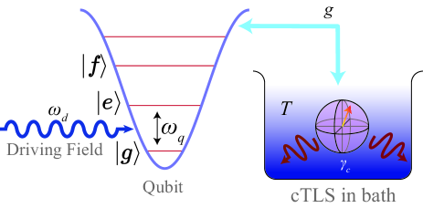
Figure 1: The system consists of an anharmonic oscillator of base level spacing $\omega_{q}$ and anharmonicity $\chi$ that models a superconducting qubit, a two-level system of spacing $\omega_{c}$ that models a near-resonant defect in the qubit junction, and a microwave driving of frequency $\omega_{d}$ to the qubit. The two-level defect is considered interacting with a thermal bath of temperature $T$ at a decay rate of $\gamma_{c}$ and simultaneously interacting with the qubit at strength $g$. The latter interaction provides a two-way channel of energy flow during the qubit thermalization process with the bath.

Considering the typical scenario where $\Omega\gg g$ ($\Omega$ in the range of MHz while $g$ in the range of hundreds of kHz for typical transmon qubits), the driving is relatively strong, compared to which the coupling to cTLS is perturbative. The discrete qubit state space can then be transformed into the continuous coherent-state space under the rotating frame of the driving $\omega_{d}$, where $\alpha_{d}=\Omega/\Delta_{d}$ denotes the amount of displacement from the vacuum state, giving $H_{q}+W(t)=D(\alpha_{d})H_{q}D^{\dagger}(\alpha_{d})$. The detuning $\Delta_{d}=\omega_{q}^{\prime}-\omega_{d}$ between the anharmonic qubit and the driving is derived from the linearized oscillator frequency $\omega_{q}^{\prime}=\omega_{q}-\chi(\bar{n}_{q}-1)$ where $\bar{n}_{q}$ denotes the average photon number in the qubit at initial state. By regarding $DH_{q}D^{\dagger}$ and $H_{c}$ as free energies in the coherent-state space, the effective qubit-cTLS coupling under the interaction picture becomes

$$H_{\mathrm{eff}}=g\left(a^{\dagger}-\alpha_{d}e^{-i\Delta_{d}t}\right)\sigma_{-}e^{i\Delta_{c}t}+\textrm{h.c.}$$ (2)

where $\Delta_{c}=\omega_{q}^{\prime}-\omega_{c}$ denotes cTLS detuning from the linearized qubit.

Given Eq. (2), the master equation of the qubit density matrix $\rho_{q}$ is derived from the Liouville equation $\dot{\rho}=-i\left[H_{\mathrm{eff}},\rho\right]$ for $\rho$ of the coupled system under the Born-Markov approximation. Exactly, the density matrix is assumed separable, i.e. $\rho(t)=\rho_{q}(t)\otimes\rho_{c}$, at initial moment before the time integration is carried out to the first perturbative order and the cTLS subsystem is traced out [supp1]. This leads to

$$\frac{\partial}{\partial t}\rho_{q}= -i\Delta_{d}\left[a^{\dagger}a,\rho_{q}\right]+\eta\left[a^{\dagger}-a,\rho_{q}\right]$$

$$+\frac{\gamma}{2}(1-\nu)\left(2a\rho_{q}a{}^{\dagger}-\left\{a^{\dagger}a,\rho_{q}\right\}\right)$$

$$+\frac{\gamma}{2}\nu\left(2a^{\dagger}\rho_{q}a-\left\{aa^{\dagger},\rho_{q}\right\}\right),$$ (3)

in the displaced $(\alpha,\alpha^{\ast})$-space. Besides the two Lindbladians contributed by direct coupling to the cTLS, the indirect coupling skewed by the driving field contributes the extra term in the second line. With $\nu=(\exp(\omega_{c}/k_{B}T)+1)^{-1}$ indicating the thermal inversion of the cTLS, the first and second Lindbladians accounts for the spontaneous qubit emission and absorption, respectively, where $\gamma=2g^{2}\gamma_{c}/(\gamma_{c}^{2}+\Delta_{c}^{2})$ is the decay rate according to the typical relaxation rate $\gamma_{c}$ of a cTLS [27]. The $\eta$ term reflects the external driving under the influence of the environment, i.e.

$$\eta =\alpha_{d}g^{2}\left[\frac{(1-\nu)\gamma_{c}}{\gamma_{c}^{2}+(\Delta_{d}+\Delta_{c})^{2}}-\frac{\nu\gamma_{c}}{\gamma_{c}^{2}+(\Delta_{d}-\Delta_{c})^{2}}\right],$$ (4)

which comprises two terms. The first term of Eq. (4) is contributed by a two-photon process where the driving field photon and the cTLS radiation photon concurrently mix with the qubit. Whereas, the second term corresponds to a one-photon process where the driving field photon bypasses the qubit and mixes with the cTLS. The resonance at the latter blocks the decay of the qubit that channels into the cTLS. It therefore adversely affects the decay depicted in Eq. (3) and has the negative coefficient. On the other hand, both terms share the common factor $\alpha_{d}$ determined by the driving amplitude. Given the environmental temperature (on the mK range) of superconducting qubits, the inversion $v$ adopts a negligible value and the existence of the driving field in general accelerates qubit relaxations (contribution of the first term $\gg$ that of the second term).

Solving for quadratures – To solve the master equation (3), we first reduce it to a Fokker-Planck (FP) equation concerning the density distribution of the qubit on the complex $\alpha$-plane. Under the $Q$-representation $Q(\alpha,\alpha^{\ast},t)=\left\langle\alpha\right|\rho_{q}(t)\left|\alpha\right\rangle/\pi$, the FP equation reads

$$\frac{\partial}{\partial t}Q= \left[\left(\bar{\nu}\gamma+i\Delta_{d}\right)\frac{\partial}{\partial\alpha}\alpha-\eta\frac{\partial}{\partial\alpha}+\mathrm{h.c.}\right]Q$$

$$+(1-\nu)\gamma\frac{\partial^{2}}{\partial\alpha\partial\alpha^{\ast}}Q,$$ (5)

where the square bracket indicates an Hermitian differential operator and $\bar{\nu}=1/2-\nu$ indicates the inversion difference between $1/2$ at infinite temperate and $\nu$ at a given temperature. To arrive at an analytical solution to Eq. (5), we first rewrite the differential equation in the real quadrature plane under a rotating frame: $x=(\alpha e^{i\Delta_{d}t}+\mathrm{h.c.})/2$ and $y=-i(\alpha e^{i\Delta_{d}t}-\mathrm{h.c.})/2$, giving

$$\frac{\partial}{\partial t}\tilde{Q} (x,y,t)=\biggl{[}\bar{\nu}\gamma\left(\frac{\partial}{\partial x}x+\frac{\partial}{\partial y}y\right)$$

$$+\frac{(1-\nu)}{4}\gamma\left(\frac{\partial^{2}}{\partial x^{2}}+\frac{\partial^{2}}{\partial y^{2}}\right)$$

$$-\eta\left(\cos\Delta_{d}t\frac{\partial}{\partial x}+\sin\Delta_{d}t\frac{\partial}{\partial y}\right)\biggr{]}\tilde{Q}(x,y,t).$$ (6)

Having the explicit oscillatory dependence in the decay rates in the second line effectively permits the separation of variable in the distribution function as $\tilde{Q}(x,y,t)=Q_{x}(x,t)Q_{y}(y,t)$, where each real quadrature follows the equations of motions

$$\frac{\partial Q_{x}}{\partial t} =\left[\bar{\nu}\gamma+\left(\bar{\nu}\gamma x-\eta\cos\Delta_{d}t\right)\frac{\partial}{\partial x}+\frac{(1-\nu)\gamma}{4}\frac{\partial^{2}}{\partial x^{2}}\right]Q_{x},$$ (7)

$$\frac{\partial Q_{y}}{\partial t} =\left[\bar{\nu}\gamma+\left(\bar{\nu}\gamma y-\eta\sin\Delta_{d}t\right)\frac{\partial}{\partial y}+\frac{(1-\nu)\gamma}{4}\frac{\partial^{2}}{\partial y^{2}}\right]Q_{y}.$$ (8)

Each equation above is essentially equivalent to a heat diffusion equation, where the first-order derivatives and the linear terms on the right hand side can be eliminated under a new space variable with the time varible transformed accordingly. The diffusion equations are analytically solvable using standard Fourier transforms. Eventually, reversing all the transforms and changes of variables, one obtains the $Q$-distribution in the complex plane

$$Q(\alpha,\alpha^{\ast},t)=\frac{1}{2\pi\sigma^{2}(t)}\exp\left\{-\frac{\left|\alpha-\mu(t)\right|^{2}}{2\sigma^{2}(t)}\right\}$$ (9)

which is Gaussian with a moving mean $\mu(t)=\mu_{ss}\exp(i\Delta_{d}t)+(\alpha_{0}-\mu_{ss})\exp(-\bar{\nu}\gamma t)$, assuming $\alpha_{0}$ as the initial coordinates. The mean converges to the asymptotic coordinates

$$\mu_{\mathrm{ss}}=\frac{\eta}{\bar{\nu}\gamma+i\Delta_{d}}-\alpha_{d}$$ (10)

at steady state, which depends on the external driving as well as the qubit decay. The variance $\sigma^{2}=\left[1-\exp(-2\bar{\nu}\gamma t)\right]\nu/4\bar{\nu}+1/2$ is expanding and convergent with time.

Classifying evolution – The evolution depicted by Eq. (9) dictates that the qubit, starting from an arbitrary (pure) coherent state $\left|\alpha_{0}\right\rangle$ for which $Q(0)\sim\mathcal{N}(\alpha_{0},1/2)$, follows a typical trajectory of decay into the quasi-coherent state $\rho_{\mathrm{ss}}$ for which $Q(t\to\infty)\sim\mathcal{N}(\mu_{\mathrm{ss}},\nu/4\bar{\nu}+1/2)$ independent of the initial state $\left|\alpha_{0}\right\rangle$. The mean $\mu_{\mathrm{ss}}$ depends only on the parameters of the driving signal and the decay parameters of the cTLS. In fact, if the driving vanishes, the equilibrium distribution $Q_{\mathrm{ss}}$ reduces to that of an equivalent thermal Gibbs state [30], which reads $\exp\left\{-|\alpha|^{2}/(\bar{n}+1)\right\}/\pi(\bar{n}+1)$ in the continuous $\alpha$-plane with $\bar{n}=\nu/2\bar{\nu}=(\exp\{\omega_{c}/k_{B}T\}-1)^{-1}$ indicating the equivalent average photon number. In other words, the qubit levels would be populated not according to $\omega_{q}^{\prime}$, but rather to the level spacing $\omega_{c}$ of cTLS regarded as an infinite-level harmonic oscillator. One therefore can follow the model in Fig. 1 and regard the qubit-cTLS interaction as a thermalization channel, for which the qubit is thermalized with a cTLS-mediated bath at the effective temperature $T_{q}=T\omega_{q}^{\prime}/\omega_{c}$. Moreover, the widened variance of $\sigma_{\mathrm{ss}}^{2}$ by $\nu/4\bar{\nu}$ compared to $\sigma^{2}(0)$ also stems from the thermal energy transferred from the cTLS to the qubit.

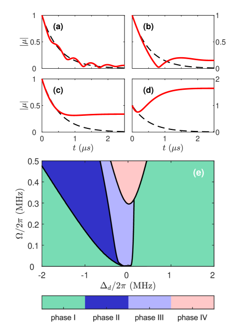
Figure 2: Dynamic phases of the decohering evolution of a superconducting qubit under driving, starting from the same initial point $\alpha_{0}=1$ in the complex $(\alpha,\alpha^{\ast})$-plane. The common parameters include the qubit frequency $\omega_{q}^{\prime}/2\pi=4.5$ GHz, the qubit-cTLS detuning $\Delta_{c}/2\pi=110$ kHz, the interaction strength $g/2\pi=400$ kHz, the cTLS relaxation rate $\gamma_{c}=1$ MHz, and the environmental temperature $T=10$ mK. The dynamic evolution exhibits distinct behaviors that can be categorized into four phases under distinct driving detunings $\Delta_{d}/2\pi$ and strengths $\Omega/2\pi$: (a) $-2$ MHz and $100$ kHz for phase I (green); (b) $-570$ kHz and $100$ kHz for phase II (deep blue); (c) $50$ kHz and $100$ kHz for phase III (light purple); and (d) $100$ kHz and $500$ kHz for phase IV (pink). The dashed curves in (a)-(d) shows the evolution of $\mu(t)$ without driving as a reference. (e) shows the partitions of these dynamic phases over a range of detunings and strengths.

For the scenario of a finite driving strength, the steady-state $Q_{\mathrm{ss}}$ has a mean $\mu_{\mathrm{ss}}$ distant from the origin, whose distribution is super-Poissonian over the displaced Fock states [31] $\left|\mu_{\mathrm{ss}},n\right\rangle$, i.e. the corresponding density matrix is

$$\rho=\sum_{n=0}^{\infty}\frac{(2\sigma_{\mathrm{ss}}^{2}-1)^{n}}{(2\sigma_{\mathrm{ss}}^{2})^{n+1}}\left|\mu_{\mathrm{ss}},n\right\rangle\left\langle\mu_{\mathrm{ss}},n\right|,$$ (11)

which would fall back to the Gibbs state described above when the driving vanishes. When the driving is present, the transient evolutions of $Q(\alpha,\alpha^{\ast},t)$ under different driving strengths and frequencies towards $Q_{\mathrm{ss}}$ are not unified but classifiable into four dynamic categories or phases: (I) oscillating, (II) collapse and revive, (III) monotonic decay, and (IV) amplifying. These phases demonstrate the competition of the external driving as a restoring energy flow against the qubit decay into the cTLS during the decohering evolution. The typical plots for these four phases of evolutions are shown in Fig. 2, along with the phase partitions over the qubit-driving detuning $\Delta_{d}$ and the driving strength $\Omega$. At near resonance, the driving becomes more effective in pushing the steady-state $\mu_{\mathrm{ss}}$ away from zero. According to the evolution of the $Q$-distribution, the energy $\left\langle H_{q}(t)\right\rangle=\hbar\omega_{q}^{\prime}(|\mu(t)|^{2}+2\sigma^{2}(t)-1)$ of the qubit varies with time in a way that if the driving is weak or far-resonant such that $|\mu_{\mathrm{ss}}|<|\alpha_{0}|$, the energy supplied by the driving to the qubit is not sufficient to cover the energy loss towards the cTLS (phase I to III). At near resonance with sufficiently large driving, however, the qubit can acculumate energy in addition to dissipating into the cTLS, exhibiting the scenario of phase IV.

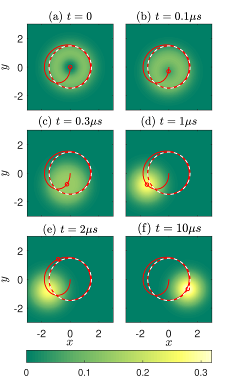
Figure 3: The evolution of the qubit $Q$-distribution plotted as contours on XY-quadrature plane, assuming a fully inverted excited state$\left|e\right\rangle$ as the initial state. The captures of six time moments are shown in the subplots, where the red curves show the trajectory of the mean $\mu(t)$ and the overlay white dashed curve indicates the limit cycle. The driving field parameters are set to $\Omega/2\pi=500$ kHz and $\Delta_{d}=-300$ kHz, where the other parameters remain the same as those in Fig. 2.

Transient dynamics – To appreciate the transient evolution of the qubit under the influence of the decohering cTLS, we consider the fully inverted $\left|e\right\rangle\left\langle e\right|$ as the qubit initial state. Its $Q$-representation $\left|\left\langle e|\alpha\right\rangle\right|^{2}/\pi$ is the continuous complex function $e^{-|\alpha|^{2}}|\alpha|^{2}/\pi$ on the $(\alpha,\alpha^{*})$ plane, which exhibits a circular-symmetric ring shape in its contour plot over the observable $XY$-quadrature plane shown in Fig. 3(a). The quadrature operators $x$ and $y$ being linear combinations of $a$ and $a^{\dagger}$, the distribution of $Q(x,y)$ shown in the plot is identical to $Q(\alpha,\alpha^{\ast})$ up to a proportional constant stemmed from the Jacobian matrix. By shrinking the initial coherent-state distribution of Eq. 9 to a point source, i.e. letting $\sigma^{2}(t)=\left[1-\exp(-2\bar{\nu}\gamma t)\right](\nu/4\bar{\nu}+1/2)$, the solution expressed by Eq. 9 represents a propagator (viz. Green function $G(\alpha|\alpha_{0},t)$) of the diffusion process from that point source. Then, the time function written as the integral $\int d^{2}\alpha\,|\alpha|^{2}\exp\{-|\alpha|^{2}\}G(\alpha|\alpha_{0},t)/\pi$ describes the entire decoherence process, the illustration of which at moments after $t=0$ are given in Figs. 3(b)-(f). The center of the distribution, marked by a red circle, shows a converging trajectory (red solid curve) towards a limit cycle of radius $|\mu_{\mathrm{ss}}|$, marked as a white dashed circle. This shows that after the dynamic balance between the driving and the energy decay to the cTLS is reached, the qubit coordinates follow the circular path at the frequency determined by the detuning $\Delta_{d}$. During the convergence, the ring-shaped distribution of variance $3\sqrt{\pi}/4$ contracts into a disk shape of variance $\nu/4\bar{\nu}+1/2$. In other words, the decoherence process is reflected as a displacement process on the quadrature plane from the origin to $|\mu_{\mathrm{ss}}|$, where the excited state distribution decays into the super-Poissonian displaced Fock state of Eq. (11).

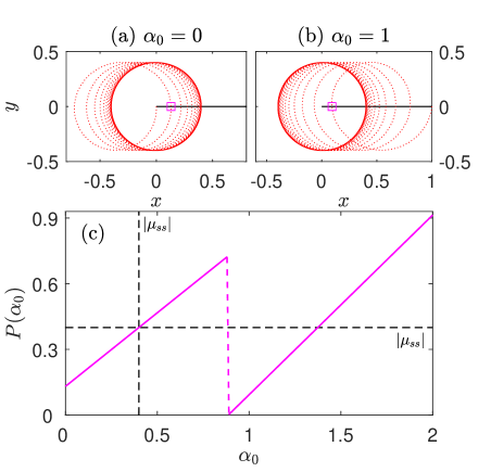
Figure 4: Trajectories of $\mu(t)$ drawn as red dotted curves on the $XY$-quadrature plane, starting from two initial points: (a) $\alpha_{0}=0$ and (b) $\alpha_{0}=1$, but under the same coupling strength $\Omega/2\pi=1$MHz and detuning $\Delta=-2.5$ MHz. The solid circles indicate the same asymptotic limit cycle of radius $|\mu_{\mathrm{ss}}|$ from the distinct initial points. The magenta squares indicate the first recurrence on the positive $x$-axis. (c) Poincare map showing the coordinate of the first recurrence as a function of initial $x$-coordinate $\alpha_{0}$. The black dashed cross shows the fixed point $\alpha_{0}=0.40$ of the recurrence function $P(\alpha_{0})=\alpha_{0}=|\mu_{\mathrm{ss}}|$. The function has two rate zones, one before and one after $\alpha_{0}=0.89$.

Not only does the driving strength $\eta$ under relaxation and the detuning $\Delta_{d}$ determine the radius of the limit cycle orbit, they also decide the rate at which the qubit state gravitates towards it. Shown in Figs. 4(a)-(b), the trajectories of $\mu(t)$ converge to the same limit cycle under identical driving conditions, but approach it under different rates when commencing from initial points of differing distance to the limit cycle. The illustrated case of $\alpha_{0}=0$ has a faster approach than that of $\alpha_{0}=1$. The generalized description of the distinct approaching rates is given conventionally by the Poincare map, shown in Fig. 4(c), where the first recurrence on the positive $x$-axis is recorded as a function $P(\alpha_{0})$ of the starting coordinate $\alpha_{0}$ on the same axis. The faster rate possessed by the starting coordinate $\alpha_{0}=0$ is associated with the situation that $P(0)$ is closer to the fixed point $P(\alpha_{0})=\alpha_{0}$, i.e. $x$ coordinate of the limit cycle, than $P(1)$. Moreover, the driving conditions determine a partition point, shown as $\alpha_{0}=0.89$ in the case illustrated in Fig. 4(c), separating a zone of first recurrence occurring at a full circle from another of first occurrence at a half circle. The former has the $P(\alpha_{0})$ function increase at a slope 0.67 while the latter 0.82.

Conclusions – We obtain an analytic description of the evolution of a superconducting qubit under the simultaneous influence of a coherent two-level system (cTLS) reflecting the role of a junction defect in a thermal bath and of an external microwave driving field. By solving a master equation in the continuous $(\alpha,\alpha^{\ast})$-plane of coherent state, we has described the thermalization process undergone by the qubit according to an effective temperature determined by the level spacing of the cTLS relative to that of the qubit. The strength of the driving competes with the couplings of the cTLS to the qubit and the environment to determine the effective qubit relaxation, which are classifiable into four phases of distinct dynamic behaviors. The competition has the qubit converge to a limit cycle of finite radius on the quadrature plane, where the rate of convergence is shown through a Poincare map.

References

- [1] G. Ithier, E. Collin, P. Joyez, P. J. Meeson, D. Vion, D. Esteve, F. Chiarello, A. Shnirman, Y. Makhlin, J. Schriefl, and G. Schön, Phys. Rev. B 72, 134519 (2005).
- [2] P. Krantz, M. Kjaergaard, F. Yan, T. P. Orlando, S. Gustavsson, and W. D. Oliver, Appl. Phys. Rev. 6, 021318 (2019).
- [3] M. J. Peterer, S. J. Bader, X. Jin, F. Yan, A. Kamal, T. J. Gudmundsen, P. J. Leek, T. P. Orlando, W. D. Oliver, and S. Gustavsson, Phys. Rev. Lett. 114, 010501 (2015).
- [4] L. B. Nguyen, Y.-H. Lin, A. Somoroff, R. Mencia, N. Grabon, and V. E. Manucharyan, Phys. Rev. X 9, 041041 (2019).
- [5] C. Müller, J. H. Cole, and J. Lisenfeld, Rep. Prog. Phys. 82, 124501 (2019).
- [6] A. D. Córcoles, J. M. Chow, J. M. Gambetta, C. Rigetti, J. R. Rozen, G. A. Keefe, M. Beth Rothwell, M. B. Ketchen, and M. Steffen, Appl. Phys. Lett. 99, 181906 (2011).
- [7] C. Neill, A. Megrant, R. Barends, Y. Chen, B. Chiaro, J. Kelly, J. Y. Mutus, P. J. J. O’Malley, D. Sank, J. Wenner, T. C. White, Y. Yin, A. N. Cleland, and J. M. Martinis, Appl. Phys. Lett. 103, 072601 (2013).
- [8] S. M. Meißner, A. Seiler, J. Lisenfeld, A. V. Ustinov, and G. Weiss, Phys. Rev. B 97, 180505 (2018).
- [9] L. Faoro and L. B. Ioffe, Phys. Rev. B 91, 014201 (2015).
- [10] P. V. Klimov, J. Kelly, Z. Chen, M. Neeley, A. Megrant, B. Burkett, R. Barends, K. Arya, B. Chiaro, Y. Chen, A. Dunsworth, A. Fowler, B. Foxen, C. Gidney, M. Giustina, R. Graff, T. Huang, E. Jeffrey, E. Lucero, J. Y. Mutus, O. Naaman, C. Neill, C. Quintana, P. Roushan, D. Sank, A. Vainsencher, J. Wenner, T. C. White, S. Boixo, R. Babbush, V. N. Smelyanskiy, H. Neven, J. M. Martinis, Phys. Rev. Lett. 121, 090502 (2018).
- [11] L. V. Abdurakhimov, I. Mahboob, H. Toida, K. Kakuyanagi, Y. Matsuzaki, and S. Saito, Phys. Rev. B 102, 100502 (2020).
- [12] S. Schlör, J. Lisenfeld, C. Müller, A. Bilmes, A. Schneider, D. P. Pappas, A. V. Ustinov, and M. Weides, Phys. Rev. Lett. 123, 190502 (2019).
- [13] Y. Lu, A. Bengtsson, J. J. Burnett, E. Wiegand, B. Suri, P. Krantz, A. F. Roudsari, A. F. Kockum, S. Gasparinetti, G. Johansson, and P. Delsing, npj Quan. Inf. 7, 1 (2021).
- [14] A. Bilmes, A. Megrant, P. Klimov, G. Weiss, J. M. Martinis, A. V. Ustinov, and J. Lisenfeld, Sci. Rep. 10, 3090 (2020).
- [15] F. Yan, S. Gustavsson, J. Bylander, X. Jin, F. Yoshihara, D. G. Cory, Y. Nakamura, T. P. Orlando, and W. D. Oliver, Nat. Commun. 4, 1 (2013).
- [16] Y. Gao, S. Jin, and H. Ian, New J. Phys. 22, 103041 (2020).
- [17] Y. Gao, S. Jin, Y. Zhang, and H. Ian, Quan. Inf. Proc. 19, 313 (2020).
- [18] T. D. Ladd, F. Jelezko, R. Laflamme, Y. Nakamura, C. Monroe, and J. L. O’Brien, Nature 464, 45 (2010).
- [19] Y. Nakamura, Y. A. Pashkin, and J. S. Tsai, Nature 398, 786 (1999).
- [20] J. Koch, T. M. Yu, Jay Gambetta, A. A. Houck, D. I. Schuster, J. Majer, A. Blais, M. H. Devoret, S. M. Girvin, and R. J. Schoelkopf, Phys. Rev. A 76, 042319 (2007).
- [21] A. A. Houck, D. Schuster, J. Gambetta, J. Schreier, B. Johnson, J. Chow, L. Frunzio, J. Majer, M. Devoret, S. Girvin, Nature 449, 328 (2007).
- [22] A. Y. Smirnov, Phys. Rev. B 67, 155104 (2003).
- [23] E. Geva, R. Kosloff, and J. Skinner, J. Chem. Phys. 102, 8541 (1995).
- [24] Z. Zhou, S.-I. Chu, and S. Han, J. Phys. B: At., Mol. Opt. Phys. 41, 045506 (2008).
- [25] J. Clarke and F. K. Wilhelm, Nature 453, 1031 (2008).
- [26] T. Orlando, J. Mooij, L. Tian, C. H. Van Der Wal, L. Levitov, S. Lloyd, and J. Mazo, Phys. Rev. B 60, 15398 (1999).
- [27] J. Lisenfeld, A. Bilmes, S. Matityahu, S. Zanker, M. Marthaler, M. Schechter, G. Schön, A. Shnirman, G. Weiss, and A. V. Ustinov, Sci. Rep. 6, 1 (2016).
- [28] H. J. Carmichael, Statistical methods in quantum optics 1: master equations and Fokker-Planck equations (Springer Science & Business Media, New York, 2013).
- A. D. Polyanin and V. E. Nazaikinskii, Handbook of linear partial differential equations for engineers and scientists [CRC press, 2015] A. D. Polyanin and V. E. Nazaikinskii, Handbook of linear partial differential equations for engineers and scientists (CRC press, Boca Raton, 2015).
- [30] R. Loudon, The Quantum Theory of Light (Clarendon Press, United Kingdom, 1973).
- [31] P. Král, Journal of Modern Optics 37, 889 (1990).
- [32] R. Keil, A. Perez-Leija, F. Dreisow, M. Heinrich, H. Moya-Cessa, S. Nolte, D. N. Christodoulides, and A. Szameit, Phys. Rev. Lett. 107, 103601 (2011).