Extremal Bounds for Three-Neighbour Bootstrap Percolation in Dimensions Two and Three
Abstract
For , the -neighbour bootstrap process in a graph starts with a set of infected vertices and, in each time step, every vertex with at least infected neighbours becomes infected. The initial infection percolates if every vertex of is eventually infected. We exactly determine the minimum cardinality of a set that percolates for the -neighbour bootstrap process when is a -dimensional grid with minimum side-length at least . We also characterize the integers and for which there is a set of cardinality that percolates for the -neighbour bootstrap process in the grid; this solves a problem raised by Benevides, Bermond, Lesfari and Nisse [HAL Research Report 03161419v4, 2021].
1 Introduction
Bootstrap percolation is a cellular automaton introduced in the late 1970s as a model of the dynamics of ferromagnetism [17]. For , the -neighbour bootstrap process (or, for brevity, the -neighbour process) is described as follows. Given a graph and an initial set of infected vertices (non-infected vertices are healthy), at each time step, a healthy vertex becomes infected if it has at least infected neighbours. That is, for , the set of vertices infected after time steps is precisely
where denotes the neighbourhood of in . The closure of with respect to the -neighbour process in is ; we simply write when and are clear from context. We say that percolates under the -neighbour process in if .
A natural extremal problem is to determine the cardinality of the smallest set of vertices which percolates under the -neighbour process in a graph , which is denoted by . Due to its origins in statistical physics, a central focus in the study of bootstrap percolation has been on the case that is a multidimensional grid [26, 31, 30, 34, 10, 22, 15, 16, 13, 3, 21, 19, 24, 35, 14, 2, 18, 9, 11, 32, 29, 6, 7, 8, 4, 5, 25]. For , let . Let denote the -dimensional grid with vertex set , where two vertices and are adjacent if there is an index such that and for all . We use the notation to refer both to the grid graph and to its vertex set. The direction of an edge of a -dimensional grid is defined to be the unique index such that differs from . For convenience, define
A beautiful exercise (featured in, e.g., [12, Problem 34]) is to show that
| (1.1) |
for all . The standard proof of the lower estimate generalizes to the following bound in any dimension :
| (1.2) |
see [30] or Proposition 2.2 in the next section. The fact that the matching upper bound to (1.2) holds has been part of the folklore of bootstrap percolation since the work of Pete [30], if not earlier. While it is not hard to recursively describe a set of cardinality that is likely to percolate, verifying this fact is technical. To our knowledge, the first published proof appears in a puzzle book of Winkler [36, pp. 97–99], where it is attributed to Schulman.111Another proof was recently published by Przykucki and Shelton [32].
Another natural generalization of (1.1) was obtained by Balogh and Bollobás [4] and applied as part of the proof of a probabilistic result for bootstrap percolation in the hypercube:
| (1.4) |
for all and .
For , tight bounds on are harder to come by. The following rough estimate for fixed and was proved by Pete [30] see [9, Section 6]):
For most choices of parameters, the best known lower bound is given by [29, Theorem 4.2 and (1.5)] (see [22] for an alternative proof and several extensions). In [29], it was proved that this lower bound is tight in the case that , and :
| (1.5) |
In this paper, we focus on the problems of computing and . Our first result is that the standard lower bound on (see Proposition 2.2) is tight, provided that the side-lengths of the grid are sufficiently large.
Theorem 1.6.
If , then
We conjecture that the hypothesis in Theorem 1.6 can be relaxed to ; see Conjecture 7.2. Briefly, the proof of Theorem 1.6 involves establishing several infinite families of optimal constructions in restricted cases and assembling them recursively using percolating sets for the so-called “modified bootstrap process” as a template.
The problem of determining for appears as a puzzle in Bollobás’ recreational mathematics book [12, Problem 65]. Recently, Benevides, Bermond, Lesfari and Nisse [10] made progress in determining the exact value of for a wider range of . In particular, they showed that
if is even and that
| (1.7) |
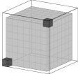
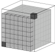
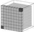
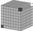
if is odd. They also showed that, in the odd case, the upper bound is tight for and the lower bound is attained when or is of the form for . The construction for of the form is particularly natural. For , we have and the unique percolating set is . Now, for , deleting the middle row and column from the grid leaves behind four subgrids. Let be an infection in the the grid obtained from taking an optimal percolating set within each of these four subgrids, plus the vertex in the centre of the grid. It is not hard to show that this infection percolates under the -neighbour process and that it it has precisely elements. See Figure 1 for an illustration. In all of the diagrams in this paper, vertices of the grid graph are represented by cells, and pairs of cells which share a boundary edge are adjacent. The point is represented by the cell on the th row (from the top) and th column (from the left). Infected cells are shown in grey; these are typically the initially infected cells in , though later it is also convenient to use grey on sets which we know will become infected later in the process.
Thus, the results of [10] nearly determined in general. The only remaining problem, proposed in [10, Section 6], was to determine whether is equal to the lower bound or the upper bound of (1.7) when is odd and not congruent to or of the form for . We complete the picture by proving that the upper bound is the truth in all such cases. This is a corollary of the following result.
Theorem 1.8.
Suppose that such that
Then there exists such that .
Corollary 1.9.
For all ,
Proof.
The first three cases follow from [10, Theorem 1] and the fact that, if , then .
Let us pause for some additional historical context. As alluded to above, bootstrap percolation is motivated in part by connections to questions originating in statistical physics. From this perspective, the most natural problem is to locate and analyze the “phase transition” of the model; i.e. to determine the density at which a random infection becomes likely to percolate. More concretely, define the critical probability of the -neighbour process in , denoted , to be the infimal value of such that a random set of vertices of sampled from the binomial distribution with parameter percolates with probability at least . As it turns out, (1.1) can be combined with a few elementary observations to obtain a short proof of a classical result of Aizenman and Lebowitz [2] that . In a groundbreaking paper of Holroyd [25], this estimate was sharpened to
| (1.10) |
where denotes the natural (base ) logarithm. Surprisingly, this bound is more than a factor of two larger than the value of predicted in the physics literature based on simulations on grids of size up to [1]. This discrepancy is explained, in part, by the fact that the second order asymptotic term of (1.10) is a negative term of order ; this was recently proved in an impressive paper of Hartarsky and Morris [24], improving on earlier estimates in [19, 20]. This second order term competes admirably with the main term until is extremely large. The breakthrough of Holroyd [25] ignited a series of tight results on the critical probability in grids of higher dimensions with different values of ; see [26, 7, 4, 8, 6, 5]. Most notably, Balogh, Bollobás, Duminil-Copin and Morris [5] determined up to a factor for all fixed as , which sharpened earlier results of [15, 16]. When , the behaviour of a random infection is very different as, in order to percolate, each -dimensional cube must contain at least one infected vertex. The analysis in this case becomes similar to that of ordinary percolation; see [23, Section 1.4.1] for more background.
In the next section, we prove the standard lower bound on and provide several key definitions. In Section 3, we present the proof of Theorem 1.8. Along the way, we build up key facts about percolating sets for the -neighbour process in -dimensional grids which will be used in Section 4 to construction percolating sets in induced subgraphs of -dimensional grids. In Section 5, we show how these percolating sets in the -dimensional setting can be “folded up” to yield optimal percolating sets in the grid for several infinite families of side-lengths . In Section 6, we feed these infinite families, and several sporadic examples from Appendix A, into a recursive lemma to complete the proof of Theorem 1.6. We conclude the paper in Section 7 by making a few final observations and stating several open problems.
2 Preliminaries
We begin by proving a simple lemma which bounds the size of the smallest percolating set for the -neighbour process in a graph in terms of its order and size and deriving a lower bound on as a corollary. Given a graph and a set , let be the number of edges of with both endpoints in . We write the neighbourhood of a vertex of simply as when the graph clear from context and let be the degree of .
Lemma 2.1.
Let be a graph and . If percolates with respect to the -neighbour process, then
Proof.
Let and . Assuming that percolates in , we can let be an ordering of the vertices of such that and, for each , the vertex has at least neighbours in . Then
The result follows by solving for in the above inequality. ∎
Next, we use Lemma 2.1 to obtain a lower bound on the cardinality of a percolating set in the grid in terms of the number of points on its boundary. In the case or , this corresponds to a lower bound in terms of the “perimeter” or “surface area” of the grid, respectively. This bound is not new. Variants of it appear in [31, 30, 12, 9], for example, and several generalizations are proved in [22, 29]. We provide a proof here for the sake of completeness.
First, we need a few definitions. For and , let
We call the th level in direction or, simply, a level for short. The sets and are called the faces in direction or just faces for short. A vertex contained in a face is called a boundary vertex. Say that a vertex is a corner if it is contained in a face in every direction .
Proposition 2.2.
Let and . If percolates with respect to the -neighbour process in , then
In particular,
Proof.
Let . By Lemma 2.1, we have that
For each vertex , the quantity is simply equal to the number of faces that belongs to (where, if for some , then we count the face twice). Thus, by double-counting, we see that is equal to the sum of the cardinalities of all of the faces of the grid; clearly, the two faces in direction each have cardinality . The result now follows by substituting in for in the above expression. ∎
For , say that a triple of positive integers is class if
A useful fact to keep in mind is that is class if and only if either at least two of and are multiples of three, or . We say that is optimal if ; that is, is optimal if the lower bound on implied by Proposition 2.2 is tight. Moreover, we say that is perfect if it is optimal and class 0. Clearly, permuting the coordinates of a triple preserves class and optimality. In this language, Theorem 1.6 says that is optimal whenever and Theorem 1.8 says that, if is perfect, then there exists an integer such that .
3 Three Neighbours in Two Dimensions
Our focus in this section is on proving Theorem 1.8. As we shall see, percolating sets for the -neighbour process in must have a very special structure; specifically, the complement of such a set must induce a forest in which each component contains at most one boundary vertex. This is a special case of a more general phenomenon, as the next lemma illustrates.
Lemma 3.1.
For , let be a graph of maximum degree at most and let . Then percolates under the -neighbour process in if and only if
-
(3.2)
contains every vertex of of degree less than and
-
(3.3)
every component of is a tree containing at most one vertex of degree .
Proof.
First, we prove the “only if” direction. Observe that any healthy vertex with at most neighbours can never become infected by the -neighbour process; therefore, if percolates, then every such vertex must be in . Now, suppose that there is a component of containing either a cycle or two vertices of degree . In either case, we can let be a walk in such that either (a) is a cycle or (b) is a path between two distinct vertices of degree . Each internal vertex of has at least two neighbours in and therefore has at most neighbours outside of . Likewise, the starting and ending vertices of also have at most neighbours outside of , regardless of whether (a) or (b) holds. Thus, by considering the first vertex of to become infected and deriving a contradiction, we see that no vertex of is infected by the -neighbour process starting with , and so does not percolate.
Now, suppose that (3.2) and (3.3) hold. We show that percolates by induction on , where the base case is trivial. Let be any component of . If , then, by (3.2), the unique has degree at least and so it becomes infected after one step; we are therefore done by applying induction to . If , then let and be distinct leaves of . By (3.3), we can assume, without loss of generality, that has degree . Since is a leaf of , it has at least neighbours in and so it is infected after one step; we are done by applying induction to once again. ∎
The following corollary is immediate from Lemma 3.1 since -dimensional grids have maximum degree at most . In this section, we are mainly interested in the “only if” direction of this corollary, but the “if” direction will be used several times in the next section.
Corollary 3.4.
For a set percolates under the -neighbour process in if and only if contains every corner and every component of is a tree containing at most one boundary vertex.
The next lemma provides some strong structural restrictions on percolating sets of cardinality in . Say that an element is even or odd depending on the parity of .
Lemma 3.5.
Let and such that . If percolates under the -neighbour process in , then
-
(3.6)
is an independent set,
-
(3.7)
every even boundary vertex is contained in ,
-
(3.8)
and are both odd,
-
(3.9)
every component of is a tree containing exactly one boundary vertex and
-
(3.10)
every is even.
Proof.
We will establish each of the properties (3.6)–(3.10) sequentially, where, in the proof of each of these statements, we may assume that all of the earlier statements hold. First, if is not an independent set, then and so applying Proposition 2.2 to which is isomorphic to , implies that , which contradicts our assumption on . So, (3.6) holds.
By Corollary 3.4, we know that no component of can contain two boundary vertices. In particular, if and are consecutive boundary vertices, then must contain at least one of or . However, by (3.6), contains at most one of or . Putting this together, we get that contains either every even boundary vertex or every odd boundary vertex. By Corollary 3.4, we know that contains every corner vertex; in particular, it contains , which is even. Thus, (3.7) holds. Now, since (3.6) and (3.7) hold and contains every corner vertex, we must have that and are even, and so (3.8) holds.
Denote the graph by . Our next goal is to show that the number of components of is equal to and use this to deduce (3.9). By Corollary 3.4, is a forest. Therefore, the number of components of is precisely
| (3.11) |
Let us now determine . By definition of , is equal to the number of edges in the grid, which is , minus the number of edges which have at least one endpoint in . By (3.6), we know that is an independent set, and so each edge has at most one endpoint in . Therefore,
We know by (3.7) and (3.6) that contains all of the even boundary vertices and all of the other vertices of have degree four. For illustration purposes, let us write where is the set of corner vertices, is the set of even boundary vertices that are not corner vertices and is the set of vertices of that are not on the boundary. Then
Clearly, and its not hard to see that . Therefore,
Putting all of this together, we get that is equal to
So, plugging this into (3.11), we get that the number of components of is
So, the number of components of is equal to . By (3.6), (3.7) and (3.8), is equal to the number of odd boundary vertices and, at the same time, every odd boundary vertex is contained in a component of . Since each component of contains at most one boundary vertex by Corollary 3.4, we see that every component of must contain exactly one odd boundary vertex; thus, (3.9) holds.
Finally, we prove (3.10). Let be the set of all odd vertices in , suppose to the contrary that is non-empty, and let . By (3.6) and (3.7), contains no boundary vertices, and so neither does . Therefore, the neighbourhood of , i.e. the set
contains a cycle. Our goal is to show that contains no vertex of which, by Corollary 3.4, will contradict the fact that percolates.
Let and and label the vertices of by so that and has at least neighbours in whenever . Suppose to the contrary that there is a vertex which is adjacent to for some . If , then this immediately violates (3.6), and so we must have . Consider the set
By our choice of vertex ordering, the vertex for has at least neighbours in . Also, has at least neighbours in , three of which are in and the other is the vertex , which is not in by assumption. Thus,
Since percolates, so does . Note that, since , we have that is divisible by three. So, by Proposition 2.2, we get
However, , simply by definition. This contradiction completes the proof of (3.10) and of the lemma. ∎
We now present the proof of Theorem 1.8.
Proof of Theorem 1.8.
We proceed by induction on . For the base case, suppose . Then every vertex of has degree at most two and so by Corollary 3.4, the only set that percolates is . From , we immediately get that . The proof in the case is symmetric.
So, from here forward, we assume and suppose that there is a set such that and percolates. By Lemma 3.5, we have that and are both odd. Let for . Our goal is to show that there is a percolating set in of cardinality . Given this, we will get that for some by induction, and so and the proof will be complete.
Let us now describe the construction of . For each , we observe that the set
which we call the tile corresponding to , must contain either one or two elements of . This is because induces a -cycle in and so by Corollary 3.4 and by (3.6). We define
The sets for partition . By (3.6) and (3.7), we have that contains precisely vertices outside of . Therefore,
Solving for yields
By (3.10), we know that, for ,
For , say that the tile is type if , type if and type otherwise; see Figure 2. We claim that there are no type tiles. To this end, suppose that is type and, using (3.9), let be the unique path in from to a boundary vertex . For , let be the unique tile containing ; in particular, . Note that there may be some indices such that and are the same tile. Also, may not be in and so it is not necessarily contained in any tile.
We claim that cannot be type . If is on the top or left face of the grid, then, by (3.7), is an odd vertex of the form or for some , respectively, and is either or . This implies that is in the tile . However, if is type , then this gives us two consecutive boundary vertices that are not in , contradicting (3.7). On the other hand, if is on the bottom or the right, then it is an odd vertex of the form or for some , respectively. However, applying (3.7) again, we see that would have to be or . Thus, both coordinates of are even, and so is the bottom right vertex of . However, since by definition, this contradicts the assumption that has type 0.
Therefore, there must exist such that is type and is not. In particular, the bottom right vertex of is in and the top left vertex of is in . Since and are adjacent, we see that cannot be to the right or below ; see Figure 3 (a). We assume that is to the left of and note that the other case is symmetric. If is type 1, then the two vertices on the right side of together with the two on the left side of induce a -cycle in the complement of which contradicts Corollary 3.4; see Figure 3 (b). So, is type . Now, we must have that is the top left vertex of and is the top right vertex of . Note that because, if is a boundary vertex, then it must be on the top face, but then would also be on the top face, thereby contradicting (3.7). The vertices to the left and below are both in and so the only possibility for is that it must be above . This implies that the tile is of type . However, we now get a -cycle in the complement of containing the top left vertex of , the bottom right vertex of and their two common neighbours in the grid (which are both odd and therefore not in by (3.10)); see Figure 3 (c) for an illustration. This contradiction completes the proof of that all tiles are type or .
Now, finally, we show that percolates in . By Corollary 3.4, this is equivalent to showing that every component of is a tree containing at most one boundary vertex. Suppose that is a walk in that forms either a cycle or a path from one boundary vertex to another. By definition of and the fact that there are no type tiles, this means that all of the tiles are of type . Therefore, for any , the subgraph of induced by is connected. So, there is a walk in from any vertex of to any vertex of that passes through all of the intermediate tiles. Using this, we either find a cycle or a or a path between two boundary vertices in which, by Corollary 3.4, contradicts the fact that percolates and completes the proof of the theorem. ∎
4 2D Shapes with Small Percolating Sets
In contrast to the previous section, which focused on non-existence results for efficient percolating sets in two dimensions, our focus in this section will be on showing that certain induced subgraphs of -dimensional grids do admit percolating sets of the smallest possible cardinality allowed by Lemma 2.1. These constructions will be applied in the next section to construct numerous optimal percolating sets in three dimensions. We start with some rather simple constructions which form the “building blocks” of more involved constructions that come later.
Lemma 4.1.
For , let such that . Then there exists a set such that and .
Proof.
Let be the set of all odd vertices of . That is, contains exactly one element from each column, alternating between the “bottom” and “top” vertex. See Figure 4 for an illustration of some small cases. It is evident that every vertex in is either in or has three neighbours in , except for the vertices and , which never become infected because they have degree 2. ∎
Lemma 4.2.
Let such that and and let
Then there exists such that and .
Proof.
Let such that . We proceed by induction on . If , then we are immediately done by Lemma 4.1; so, we assume . By induction, there exists a set of cardinality such that the closure of contains all of except for the point and , where is the unique element of . We let be the subset of consisting of the elements of along with and a subset of of cardinality such that consists of all of except for the point and . Then
The fact that has the desired closure is not hard to see; an illustration is provided in Figure 5. First, run the -neighbour process in each of and separately. After doing so, the graph obtained by deleting the infected vertices consists of the corners and and trees (in fact, one path and two singletons) which each contain a unique boundary vertex. Thus, we are done by Lemma 3.1. ∎
Lemma 4.3.
Let and such that and . Then there is a set such that and .
Proof.
Finally, we will start to consider infections whose closures leave behind more than just corner vertices.
Lemma 4.4.
Let and , then there is a set such that and contains all of except for the following:
Proof.
In the case that , we use Lemma 4.2 to get a set of cardinality whose closure contains all of except for and . Now, let . Then since and it is not hard to see that has the correct closure; see Figure 6 (a).
So, we assume that . Let and note that . By Lemma 4.2, there is a set of cardinality such that the closure of contains all but the corners and . By the result of the previous paragraph, there is a subset of of cardinality whose closure contains all but . We let . Then
To see that has the correct closure is a simple application of Lemma 3.1; see Figure 6 (b). ∎
Lemma 4.5.
Let and such that and . Then there is a set such that and contains all of except for the following:
Proof.
Applying Lemma 4.1, we get a set of cardinality in whose closure contains all points of this grid except for and . Also, by Lemma 4.4, we get a set in of cardinality whose closure contains all elements of this grid except for and . Putting these two constructions together with an additional infection on yields a set with the desired closure of cardinality
Lemma 4.6.
If and , then there is a set such that and contains all of except for the following:
Proof.
Since and is odd, Lemma 4.3 tells us that there is a subset of of cardinality whose closure contains all of this grid except for the corners and . Also, since by Lemma 4.2, there is a subset of of cardinality whose closure contains all of this grid except for and . We take these two constructions and add two additional infected points: and . It is not hard to see that this infection has the desired closure; see Figure 7. The cardinality of this set is
Lemma 4.7.
Let so that and . Then there is a set such that and contains all of except for the 11 elements of the following set:
Proof.
By Lemma 4.2, we can take a subset of of cardinality whose closure contains all of this grid except for the corners and . Also, by Lemma 4.1, there is a subset of the grid of cardinality whose closure contains all of this grid except for and . We take the union of these two sets together with the point . It is an easy application of Lemma 3.1 to show that this set has the correct closure; see Figure 8. The cardinality of this set is
5 Folding 2D Shapes Into the Third Dimension
Our aim in this section is to present a strategy for “folding” the constructions from the previous section into three dimensions to yield a percolating set in . Some of the arguments involve showing that the folded -dimensional structure “separates” the two faces in direction for all ; the following lemma shows that this is sufficient.
Lemma 5.1.
For and , let be a subset of . If, for every , every path in between the two faces in direction contains a vertex of , then percolates under the -neighbour process in .
Proof.
We proceed by induction on , where the base case is trivial. Let be any component of the subgraph of induced by . By the hypothesis of the lemma, for each , we have that either or . Without loss of generality, for all . Now, let be the lexicographically minimal element of . Then, for every , we see that is adjacent to a vertex of via an edge in direction . Thus, if the vertices of are infected, then becomes infected in the first step of the -neighbour process. The result follows by applying the induction hypothesis to . ∎
Let us now explain the manner in which we implant -dimensional structures into -dimensional grids. Given graphs and , a local embedding of into is a function such that whenever (i.e. is a homomorphism) and, for each , the restriction of to is injective. We remark that most, but not all, of the local embeddings used in this section will actually be injective on their entire domain.
Lemma 5.2.
Let and be graphs, let and let . If is a local embedding of into , then .
Proof.
Let be the cardinality of and let be the vertices of ordered so that and, if , then has at least neighbours in . Clearly, contains for all . Since is a local embedding, for each , the vertex has at least neighbours in . Thus, contains for all and the lemma follows. ∎
Our aim in the rest of this section is to use Lemmas 3.1, 5.1 and 5.2 to demonstrate that many tuples for are perfect. Most of the arguments follow the same general pattern. First, we exhibit a set which percolates under the -neighbour process in an induced subgraph of a -dimensional grid; we call an induced subgraph of a -dimensional grid a grid graph for short. Second, we describe a local embedding of into . Third, we argue that either the image of under the local embedding separates the faces of in direction for all , or that this property is satisfied after adding a few more infected vertices and/or performing a few steps of the -neighbour process, and so percolation occurs by Lemma 5.1. In some cases, the third step is replaced by an argument showing that the set percolates without appealing to Lemma 5.1. In fact, some of the proofs do not follow these three steps at all.
As in the previous section, many of the proofs are best explained with a series of accompanying diagrams. In these diagrams, the way that we depict an grid in this section is as copies of an grid listed left to right.222Particularly large constructions are sometimes written on two lines. The first grid on the second line is viewed as being immediately to the right of the last one on the first line. Each square in an grid is viewed as being directly above the corresponding square in the grid to the right of it and below the corresponding square in the grid to the left of it. In some of these diagrams, some of the non-grey squares contain numbers corresponding to the number of steps the corresponding vertex takes to become infected. In other words, each square containing a is adjacent to three grey squares and, for , each square containing the number is adjacent to three squares which are either grey or contain a number less than , at least one of which contains the number . We also indicate local embeddings by diagrams in which each cell is labelled by the image of the vertex that it is mapped to.
As discussed in the previous paragraph, many of our arguments involves running the -neighbour process to starting with a set that percolates in a grid graph , mapping into via a local embedding, and then running the -neighbour process in with the image of (perhaps with a few additional infections added) as the starting infection. For this reason, most of the diagrams depicting infections in 3-dimensional grids actually show the full image of a grid graph under a local embedding in grey; e.g., Figure 9 (c) shows the image of in Figure 9 (a) under the local embedding described in Figure 9 (b).
Proposition 5.3.
If and , then is perfect.
Proof.
For the purposes of presenting the diagrams, we will work in the grid for . Let us first consider the case . Our goal is to construct a percolating set of cardinality . Consider first the grid graph in Figure 9 (a). The infection depicted in the figure percolates in by Corollary 3.4. Figure 9 (b) describes a local embedding of into . By Lemma 5.2, if the 10 vertices of the image of the initial infection in under the embedding are infected in , then the image of every vertex of under the embedding eventually becomes infected. The image of under this embedding is depicted in Figure 9 (c). In Figure 9 (d), it is shown that the set obtained by adding and to the image of percolates in . Thus, there is a percolating set of cardinality .
For , let be the grid graph obtained from by inserting a grid in the location of the bold vertical line in Figure 9 (a). Using Lemma 4.2, we place an infection of cardinality in the first columns of this inserted grid whose closure leaves behind only the top left and top right corner. We also infect the vertex on the first row of the last column of the inserted grid. The infection on the rest of is the same as in . See Figure 10 for an illustration of the infection in after taking the closure of the infection on the first columns of the inserted grid. It is easily observed that, after taking the closure of the infection on the first columns of the inserted grid, the complement of the infection consists of trees, each of which contains a unique vertex of degree three in . So, by Lemma 3.1, this infection percolates in . By construction, its cardinality is
The local embedding of into is analogous to the local embedding of into . Specifically, the vertices on the top row of the inserted grid are mapped to from left to right. The vertices on the second, third and fourth rows are mapped to , and from left to right, respectively. The vertices to the right of the inserted grid are mapped to the same vertex as they are under the embedding of , except that the second coordinate is increased by . The embedding in the case is provided in Figure 10 (b) for reference. As in the case , by adding two additional infected points, namely and , to the image of under the local embedding, we obtain a set which percolates under the -neighbour process in . To formally prove this, one can observe that, after three steps of the process, there are no paths between the two faces in direction for any , and so percolation occurs by Lemma 5.1. An illustration in the case is given in Figure 10 (c). Thus, , as desired. ∎
Proposition 5.4.
If and , then is perfect.
Proof.
In all diagrams in this proof, we view the grid as for . Let be the grid graph depicted in Figure 11 (a). Between the two bold vertical lines is a grid with the top right corner removed. For , let be the grid graph obtained from by replacing this grid with the top right corner removed with a grid with the top right corner removed.
By Lemma 4.2, we can infect a set of points within a grid whose closure contains all elements of the grid except for those in the first column, the top vertex in the second column and the top right vertex. We infect those elements in the copy of the grid with the top corner removed within . Also, we infect the vertex on the first row and column of this particular grid graph within . The infection on the elements of outside of this grid are depicted in Figure 11 (a). By Lemma 3.1, this infection spreads to every element of . Figure 11 (b) describes a local embedding of into ; the embedding of for general is analogous. Figure 11 (c) verifies that the image of all vertices of under this local embedding percolates under the -neighbour process. In general, the argument goes as follows. Each vertex of the form for is adjacent to and , each of which is in the image of under the local embedding. Additionally, is adjacent to , which is also in the local embedding. Using this, we see that every vertex of the form for becomes infected. Also, becomes infected due to it being adjacent to and , all of which are in the image of . Now that and are infected, becomes infected as well, due to its adjacency to . At this point, we can invoke Lemma 5.1 to get that percolation occurs. Thus,
as desired.
∎
An exhaustive computer search easily concludes that is not perfect. Therefore, the condition that is larger than is necessary in Proposition 5.4. The following Corollary summarizes Propositions 5.3 and 5.4.
Corollary 5.5.
is perfect if and only if and .
Proof.
Proposition 5.6.
Let . If and , then is perfect.
Proof.
Without loss of generality, we assume that and . In our diagrams, we view the grid as for convenience. Let be the grid graph obtained from a grid by adding a cell to the left of the bottom left cell and deleting the bottom five cells in the rightmost column. By applying Lemma 4.5, and adding an additional infection on the added cell, we get a percolating set in of cardinality . See Figure 12 (a) for an illustration in the case and .
We define a local embedding of into as follows. For , the first vertices on the th row are mapped to from left to right and the last vertex on the th row is mapped to . For , the verties on the th row are mapped to from left to right. For , the vertices on the th row, excluding the extra vertex added on the last row, are mapped to . Finally, the extra vertex on the last row is mapped to . See Figure 12 (b) and (c) for an illustration of the embedding and the image of under that embedding, respectively, in the case and . Starting with the image of fully infected, the vertices and each have three infected neighbours. Thus, they become infected after one additional step of the -neighbour process; each of these vertices is marked with an X in Figure 12 (c). Upon infecting these two vertices, we see that there is no path between the two faces in any of the three possible dimensions which avoids the current infection. Thus, percolation occurs by Lemma 5.1. We conclude that for all such and , which is exactly what we set out to prove.
∎
Proposition 5.7.
Let . If and , then is perfect.
Proof.
Without loss of generality, and . In our diagrams, we view the grid as . Let be the graph obtained from the grid by deleting the points
By Lemma 4.6, has a percolating set of cardinality . A local embedding of into in the case that and is given in Figure 13 (a); the local embedding in the general case is analogous. The percolating set consists of the image of the aforementioned infection in under this local embedding together with the points in the set
Consider the set consisting of the elements of the union of and the image of under the local embedding contained within . Then the elements of contained in percolate within , as shown in Figure 13 (b). After running the -neighbour process within the image of and within , it is easily observed that the resulting infection percolates. In particular, after running the process for three additional time steps, we reach an infection in which there are no paths between the two faces in any of the three directions. See Figure 13 (c) for an illustration of these final stages of the process when and . ∎
Proposition 5.8.
If and , then is perfect.
Proof.
We view the grid as . Define
Also, for , define
Let . Clearly,
So, it suffices to show that percolates. The case is shown in Figure 14 (a) and so we focus on the case . The case is displayed in Figure 14 (b) for reference.
First, observe that all elements of the grid , except for and , become infected in one step. Likewise, all elements of get infected in one step, except for ; note that the infection of uses the fact that is in . The vertices and also get infected in just one step. After infecting these vertices, we see that each vertex of the form for is adjacent to and , each of which is currently infected. Additionally, is adjacent to , which is also infected. Thus, we see that all of for become infected, one after the other.
Each vertex for is now adjacent to infected vertices and . Additionally, is adjacent to , which is currently infected. So, all of for get infected. After this, becomes infected due to having infected neighbours and .
Now, we observe that becomes infected due to being adjacent to , and , each of which is either in or was infected after one step. Using this, we get that and also get infected. Also, each of for become infected, one by one.
Currently, all of is infected, except for and . It is now not hard to see that all of the remaining uninfected vertices of (i.e. the top row and the rightmost two vertices on the second row) become infected, one at a time. This triggers the last two vertices in to become infected. Finally, it becomes easy to see that all of becomes infected. This completes the proof. ∎
Proposition 5.9.
If and , then is perfect.
Proof.
In the case that , the result follows from Proposition 5.8. So, from here forward, we assume that . In our diagrams, we view the grid as . Let be a grid with and removed. By Lemma 4.2, there is an infection of cardinality in whose closure contains all but the corners and . By inspecting the proof of Lemma 4.2, we observe that this set contains and and does not contain .333In fact, rather than inspecting the proof, one could alternatively apply Lemma 3.1 to show that any such infection must alternate around the boundary of , analogous to the proof (3.7). Also, since has only three neighbours, it does not become infected until after becomes infected. Thus, this construction gives us a percolating set in of cardinality .
An illustration of a local embedding of into in the case is given in Figure 15 (a); the local embedding in the general case is analogous. Note that, in contrast to the previous proofs in this section, this local embedding is not injective. Specifically, it maps both of and to . Recall that both of and were contained in the initial infection of . Thus, the image of the infection in under the local embedding has cardinality . We add six additional elements to the infection: and . It is tedious, but not difficult, to show that this set percolates. See Figure 15 (b) for an illustration in the case that ; in this figure, the six additional infections are marked with an X and the other grey cells are the elements of the image of under the local embedding. Thus,
as desired. ∎
Proposition 5.10.
If and , then is perfect.
Proof.
In the case that , the result follows from Proposition 5.3. So, from here forward, we assume that . We view the grid as . Define
Also, for , define
Also, let . We have
So, it suffices to show that percolates. See Figure 16 for a depiction of the case .
First, note that every vertex within becomes infected in one step except for ; note that the infection of uses the fact that is in . Similarly, every vertex of becomes infected after one step, and every vertex of becomes infected after one step, except for .
At this point, each vertex of the form for is adjacent to infected vertices and . In addition, is adjacent to , which is in . So, all of the vertices for become infected. Once these vertices are infected, we see that the vertices for become infected in a similar manner. The vertex now has infected neighbours and and so it becomes infected, and then becomes infected as well. In a very similar way, the infection spreads to all vertices in . Now, all vertices of are infected and it is not hard to see that the other two layers eventually become infected as well. ∎
Proposition 5.11.
If and , then is perfect.
Proof.
In the case that , the result follows from Proposition 5.8. So, from here forward, we assume that . We view the grid as . Define
Also, for , define
Now, let . We have
Let us show that percolates. See Figure 17 for a depiction of the case .
First, observe that all vertices of becomes infected in one step, apart from ; the infection of uses the fact that is in . Similarly, all of becomes infected in one step and all of except for becomes infected.
At this point, each vertex of the form for is adjacent to infected vertices and . Additionally, is adjacent to , which is in . So, each vertex of the form for becomes infected, one after the other. Likewise, each vertex of the form for becomes infected, as does each vertex of the form for . Each vertex of the form for also gets infected; this time, the infection does not spread immediately to because is not currently infected.
At this point, we have shown that every vertex in becomes infected, except for and seven vertices in . It is not hard to see that these eight vertices all become infected; see Figure 17 for an illustration of this. Now, once all of is infected, it is not hard to see that the other two levels also become infected. This completes the proof. ∎
We can now characterize the perfect triples of the form .
Corollary 5.12.
is perfect if and only if .
Proof.
Proposition 5.13.
If , and , then is perfect.
Proof.
In our diagrams, we view the grid as . Let be the grid graph obtained from by deleting all of the points such that either or ; see Figure 18 (a) for the case and . By Lemma 4.7, there is a percolating set in of cardinality . A local embedding of into in the case and is provided in Figure 18 (a); the local embedding in the general case is analogous. The percolating set that we consider is the image of the aforementioned percolating set in under the local embedding together with the point ; the case and is shown in Figure 18 (b), where the additional point is labelled with an X. The cells in that figure labelled with Y are infected after one step of the -neighbour process. At this point, we can invoke 5.1 to get that this set percolates. The cardinality is , as desired. ∎
The following corollary characterizes the perfect triples of the form .
Corollary 5.14.
is perfect if and only if .
6 Recursive Constructions
To complete the proof of Theorem 1.6, we will blend together the constructions from the previous section and a few sporadic examples from Appendix A using a recursive strategy to show that we can handle all sufficiently large choices of parameters. This recursive strategy makes use of the so-called modified bootstrap process in , which is similar to the -neighbour process except that a vertex becomes infected if it is adjacent to infected vertices via at least one edge in all of the possible directions. For instance, in two dimensions, a vertex becomes infected if it has at least one infected neighbour to the North or South and at least one to the West or East, but does not become infected if it only has one to the West and one to the East. This process is fairly well studied; in particular, Holroyd [25, 26] obtained sharp estimates on the critical probability of this process.
We state the following lemma in full generality, but remark that we will only apply it in the cases and . This special case is highlighted by the corollary that follows it.
Lemma 6.1.
For and , let be a matrix of positive integers and, for , let . Let be a percolating set for the modified bootstrap process in and, for each , let be a percolating set for the -neighbour process in . Then
Proof.
We view the cube as being partitioned into cubes by viewing the th dimension as being partitioned into intervals of length and considering products of these intervals. Formally, for , we let be the grid with vertex set
We note that is isomorphic to the cube .
Now, for every , suppose that we infect the vertices of corresponding to the vertices of under the natural isomorphism from to . Let be the set of all such vertices. To see that percolates in , we start by running the -neighbour process for steps where is the minimum integer such that . Such an integer clearly exists by construction of .
Our final task is to show that percolates in . Let be the vertices of listed so that are the vertices of and, for , has neighbours in via edges in at least different directions. Now, for , we show that every vertex of is eventually infected by induction on . As we concluded in the previous paragraph, every vertex of for is in ; this settles the base case. For , without loss of generality, contains the neighbour of whose th coordinate is smaller than the th coordinate of for all . Let be the grid with vertex set
By induction on , for every , at least one of the faces of in direction eventually becomes fully infected. Thus, by Lemma 5.1, eventually becomes fully infected, and so becomes fully infected. This completes the proof. ∎
The following corollary describes the main way in which we apply Lemma 6.1.
Corollary 6.2.
Let be a matrix of positive integers. Let for . Then is at most
Moreover, if is optimal and each of the triples , is perfect, then is optimal.
Proof.
The general upper bound on follows from Lemma 6.1 since the vertices and form a set which percolates under the modified bootstrap process in . Regarding the “moreover” part of the statement, we observe that, if is optimal and all of , and are perfect, then can be rewritten as
This completes the proof. ∎
We remark that, in order to apply Lemma 6.1 to obtain optimal bounds (as in Corollary 6.2), one requires a percolating set of cardinality for the modified bootstrap process in . For , this is a triviality, as we saw in the proof of Corollary 6.2. For larger , it seems likely that the construction in the proofs of [36, 32] of the matching upper bound to (1.2) actually percolates under the modified process; however, we have not verified this. If so, then their construction can be used in Lemma 6.1. However, Corollary 6.2 will be sufficient for us.
In the special case that is class zero, we will prove the following stronger form of Theorem 1.6.
Theorem 6.3.
If and is class , then
As a simple application of Corollary 6.2, let us now derive Theorem 1.6 from Theorem 6.3; the rest of the section will then be devoted to proving Theorem 6.3.
Proof of Theorem 1.6.
Let be given and choose such that for all . Also, define for . Our goal is to argue that all of and are perfect and that is optimal. Given this, we will be done by Corollary 6.2.
By definition, each of and is a multiple of three. Therefore,
are all class zero. Also, by definition, and the fact that , all of the integers for are at least . Therefore, by Theorem 6.3, and are perfect.
Thus, all that remains is to show that is optimal whenever . If or two of are equal to , then is class and so, in these cases, the result follows from Theorem 6.3.444Note that the case also follows from Theorem 1.3. Up to symmetry, the remaining cases are and . Ad hoc constructions (found by computer) for each of the first four cases are provided in the appendix as Constructions A.6, A.7, A.8 and A.9, respectively. For the case , we apply Corollary 6.2 with
For this, we use the fact that the tuples and are perfect by Corollary 5.14 and is optimal by Construction A.5. ∎
Our final goal is to prove Theorem 6.3. The following lemma allows us to reduce to the case that one of is in .
Lemma 6.4.
Suppose . If is optimal, then is optimal. Moreover, if is perfect, then is perfect.
Proof.
We now deal with the cases in which is equal to or separately.
Lemma 6.5.
If is class 0 and , then is perfect.
Proof.
In order for to be class , we must have or . Our argument applies Corollary 6.2 to various choices of four perfect triples according to the values of and .
Suppose and each is at least . If , we set up an application of Corollary 6.2 using the triples
The first of these is perfect from doubling via Corollary 6.2. The second triple in the list is perfect from either Corollary 5.5 (if one of or equals 9) or Proposition 5.7 (if both are at least ). Finally, the last two triples are perfect from Corollary 5.12. Using these in Corollary 6.2, it follows that is perfect. On the other hand, if , we instead use
appealing to Corollary 5.5, Proposition 5.7, Corollary 5.14 and Corollary 5.12. This list of triples also works for and any , where here Corollary 5.5 is used for the second triple. Up to reordering, the remaining cases are . The first of these is obtained using the perfect triples (two of each) in Corollary 6.2. Finally, a construction for is given in Construction A.4.
Suppose . If and , then we apply Corollary 6.2 using the triples
The second triple is perfect from Proposition 5.6 and the last two are perfect via Corollary 5.5. The same construction also works for ; in this case, the second triple is , which we recall is also perfect.
On the other hand, if have the same parity with one strictly larger than , say , then we apply Corollary 6.2 using the perfect triples
A construction for appears in Construction A.1, and otherwise the same results as above apply. These triples also work for , provided . For the remaining cases, is perfect by Theorem 1.3, and a construction for is given in Construction A.3. ∎
Lemma 6.6.
If is class 0 and , then is perfect.
Proof.
In order for to be class 0, at least one of or must be divisible by three. First, suppose that and are both even. Then, by Proposition 5.13 and the fact that and at least one of or is a multiple of , we get that each of the following four triples is perfect:
It follows that is perfect by Corollary 6.2.
Next, suppose that is even with , and is odd with . Consider the four triples
These are seen to be perfect from, respectively, Proposition 5.8, Proposition 5.13 (noting that at least one of or is ), Proposition 5.8, and Corollary 5.12. Again, is perfect by Corollary 6.2.
Suppose now that and are both odd and both at least 9. We again apply Corollary 6.2, this time on the triples
These are seen to be perfect from the same set of results as above.
The only cases left to consider have one parameter equal to ; suppose without loss of generality that . Since is class 0, must be divisible by 3. If is even, then by Propositions 5.13 and 5.9, each of the following four triples is perfect:
If is odd, then the triples
are perfect by, Propositions 5.8, 5.9, 5.13 and 5.10, respectively. In either case, is perfect by Corollary 6.2. This completes the proof of the lemma. ∎
Lemma 6.7.
If is class 0 and , then is perfect.
Proof.
For to be class , we must have or . We proceed as in the proofs of the previous two lemmas.
Suppose and each is at least . We apply Corollary 6.2 using the triples
The first triple is perfect via Corollary 5.14, and the second is perfect from Lemma 6.5. The third and fourth triples are perfect from Corollary 5.5.
Next, we consider the case . Suppose first that . If , we decompose into triples
These are perfect from Theorem 1.3, Corollary 5.14, and Proposition 5.9 (twice), respectively. If , we proceed similarly using
The first of these is perfect from Corollary 6.2 applied to and ; the second is perfect again via Corollary 5.14.
In view of the above, we may assume in what follows that . If , we use a decomposition into triples
Construction A.2 shows that is perfect, the second triple is perfect from Proposition 5.6, and the last two are perfect from Lemma 6.5. Suppose now that have the same parity and , say without loss of generality . In this case, we use perfect triples
with similar ingredient results as above. The remaining case is settled using perfect triples (twice each). This completes the proof of the lemma. ∎
We are now ready to establish our result for perfect triples.
7 Conclusion
We conjecture that Theorem 1.6 generalizes to higher dimensions.
Conjecture 7.1.
For every , there exists a positive integer such that if
then
Also, in the case , we conjecture that Theorem 1.6 can be extended to nearly any choice of parameters .
Conjecture 7.2.
If , then
When one or more of the parameters are very small, the conclusion of Conjecture 7.2 no longer holds. For example, Theorem 1.8 implies that, if , then it it fails to hold for a vast majority of . It is also not hard to show that any percolating set for the -neighbour process in must contain at least three infected points on any two consecutive levels. Therefore,
whereas the lower bound from Proposition 2.2 is , and so is not optimal for large . At the same time, it seems that the conclusion of Conjecture 7.2 could be true when , and is relatively large. The smallest class tuple of the form which we have been unable to show is perfect is . We will not speculate on the exact characterization of optimal triples , but note that it would be interesting to determine it.
While Corollary 1.9 determines exactly for all , it leaves open the problem of determining the optimal size of a percolating set in a general -dimensional rectangular grid.
Problem 7.3.
Determine for all .
In [34], it was shown that the number of optimal percolating sets for the modified bootstrap process in is counted by the Schröder Numbers (OEIS A006318 [27]). The related problem of bounding the number of optimal percolating sets for the -neighbour process in is an intriguing open problem which, to our knowledge, was first posed by Bollobás (unpublished). In another direction, it would be interesting to bound the number of optimal percolating sets for the modified bootstrap process in .
Problem 7.4.
Enumerate or approximate the number percolating sets of cardinality for the modified bootstrap process in .
Of course, the generalization of Problem 7.4 to for all is also interesting. In another direction, one could consider the asymptotics for a fixed value of as . Note that every percolating set of order for the modified bootstrap process in contains exactly one point in every line parallel to any of the three axes. That is, each percolating set corresponds to a Latin square. This is analogous to the -dimensional case in which each optimal percolating set for the modified process corresponds to a permutation matrix. However, if the two dimensional case is anything to go by, then one should expect the number of percolating sets to be far smaller than the number of Latin squares (the growth rate of the Schröder Numbers is [27]). Table 1 lists the number of optimal percolating sets for the modified process in for small values of ; these were found via an exhaustive computer search. For comparison, we also include the number of Latin squares of order , as reported in OEIS A002860 [28].
| # of percolating sets | # of Latin squares | |
|---|---|---|
| 1 | 1 | 1 |
| 2 | 2 | 2 |
| 3 | 12 | 12 |
| 4 | 256 | 576 |
| 5 | 2688 | 161280 |
| 6 | 148958 | 812851200 |
Let us conclude by mentioning a consequence of Theorem 1.6 and one more open problem. For , define to be the graph obtained from by adding an edge from to if there exists such that , and for all . The graph is referred to as a -dimensional torus. In [10, Theorem 2], it is shown that
| (7.5) |
for all . A general lower bound on can be derived from the combination of [29, Equation (1.5)] and [22, Theorem 8]. In the case , this bound reduces to
| (7.6) |
for all . As a corollary of Theorem 1.6, we show that this bound is within 1 of the truth, provided that are large enough.
Corollary 7.7.
If , then
Proof.
By Theorem 1.6, there is a percolating set of cardinality
for the -neighbour process in . We let be the set obtained from by adding the points and . We show that percolates in . See Figure 19 for an illustration of four key stages of the infection.
Using , we see that all vertices of eventually become infected. Now, each vertex of the form for and is adjacent to the infected vertices and in the torus. Additionally, is, itself, infected. So, the infection eventually spreads to every vertex of the form for and .
At this point, each vertex of the form for has infected neighbours and . Additionally, is adjacent to the vertex , which is in . So, each vertex of the form for becomes infected. Likewise, each vertex of the form for becomes infected.
Now, each vertex of the form for and has two infected neighbours, namely and . Moreover, each of the vertices for has another infected neighbour, namely . So, all vertices of the form for and become infected. Symmetrically, every vertex of the form for and gets infected. The remaining healthy vertices are for . Each of these vertices currently has more than three infected neighbours and so they all become infected.
∎
Thus, (7.6) and Corollary 7.7 narrow down to only two possible values when are at least 12. It would be interesting to determine which of these two values is correct for large .
Problem 7.8.
Determine for all sufficiently large.
Of course, it would be even more interesting to determine exactly for all choices of and . Additional open problems can be found in the Master’s Thesis of the third author [33].
References
- [1] J. Adler, D. Stauffer, and A. Aharony. Comparison of bootstrap percolation models. J. Phys. A, 22:L297–L301, 1989.
- [2] M. Aizenman and J. L. Lebowitz. Metastability effects in bootstrap percolation. J. Phys. A, 21(19):3801–3813, 1988.
- [3] P. Balister, B. Bollobás, M. Przykucki, and P. Smith. Subcritical -bootstrap percolation models have non-trivial phase transitions. Trans. Amer. Math. Soc., 368(10):7385–7411, 2016.
- [4] J. Balogh and B. Bollobás. Bootstrap percolation on the hypercube. Probab. Theory Related Fields, 134(4):624–648, 2006.
- [5] J. Balogh, B. Bollobás, H. Duminil-Copin, and R. Morris. The sharp threshold for bootstrap percolation in all dimensions. Trans. Amer. Math. Soc., 364(5):2667–2701, 2012.
- [6] J. Balogh, B. Bollobás, and R. Morris. Bootstrap percolation in three dimensions. Ann. Probab., 37(4):1329–1380, 2009.
- [7] J. Balogh, B. Bollobás, and R. Morris. Majority bootstrap percolation on the hypercube. Combin. Probab. Comput., 18(1-2):17–51, 2009.
- [8] J. Balogh, B. Bollobás, and R. Morris. Bootstrap percolation in high dimensions. Combin. Probab. Comput., 19(5-6):643–692, 2010.
- [9] J. Balogh and G. Pete. Random disease on the square grid. In Proceedings of the Eighth International Conference “Random Structures and Algorithms” (Poznan, 1997), volume 13, pages 409–422, 1998.
- [10] F. Benevides, J.-C. Bermond, H. Lesfari, and N. Nisse. Minimum lethal sets in grids and tori under 3-neighbour bootstrap percolation. Technical report, 2021. HAL Research Report 03161419v4.
- [11] F. Benevides and M. Przykucki. Maximum percolation time in two-dimensional bootstrap percolation. SIAM J. Discrete Math., 29(1):224–251, 2015.
- [12] B. Bollobás. The art of mathematics. Cambridge University Press, New York, 2006. Coffee time in Memphis.
- [13] B. Bollobás, H. Duminil-Copin, R. Morris, and P. Smith. The sharp threshold for the Duarte model. Ann. Probab., 45(6B):4222–4272, 2017.
- [14] B. Bollobás, P. Smith, and A. Uzzell. Monotone cellular automata in a random environment. Combin. Probab. Comput., 24(4):687–722, 2015.
- [15] R. Cerf and E. N. M. Cirillo. Finite size scaling in three-dimensional bootstrap percolation. Ann. Probab., 27(4):1837–1850, 1999.
- [16] R. Cerf and F. Manzo. The threshold regime of finite volume bootstrap percolation. Stochastic Process. Appl., 101(1):69–82, 2002.
- [17] J. Chalupa, P. L. Leath, and G. R Reich. Bootstrap percolation on a Bethe lattice. J. Phys. C, 12:L31–L35, 1979.
- [18] A. C. D. van Enter. Proof of Straley’s argument for bootstrap percolation. J. Statist. Phys., 48(3-4):943–945, 1987.
- [19] J. Gravner and A. E. Holroyd. Slow convergence in bootstrap percolation. Ann. Appl. Probab., 18(3):909–928, 2008.
- [20] J. Gravner, A. E. Holroyd, and R. Morris. A sharper threshold for bootstrap percolation in two dimensions. Probab. Theory Related Fields, 153(1-2):1–23, 2012.
- [21] J. Gravner, A. E. Holroyd, and D. Sivakoff. Polluted bootstrap percolation in three dimensions. Ann. Appl. Probab., 31(1):218–246, 2021.
- [22] L. Hambardzumyan, H. Hatami, and Y. Qian. Lower bounds for graph bootstrap percolation via properties of polynomials. J. Combin. Theory Ser. A, 174:105253, 12, 2020.
- [23] I. Hartarsky. Bootstrap percolation and kinetically constrained models: two-dimensional universality and beyond. PhD thesis, CEREMADE, Université Paris Dauphine, PSL, Paris, France, 2022.
- [24] I. Hartarsky and R. Morris. The second term for two-neighbour bootstrap percolation in two dimensions. Trans. Amer. Math. Soc., 372(9):6465–6505, 2019.
- [25] A. E. Holroyd. Sharp metastability threshold for two-dimensional bootstrap percolation. Probab. Theory Related Fields, 125(2):195–224, 2003.
- [26] A. E. Holroyd. The metastability threshold for modified bootstrap percolation in dimensions. Electron. J. Probab., 11:no. 17, 418–433, 2006.
- [27] OEIS Foundation Inc. The On-Line Encyclopedia of Integer Sequences, 2022. https://oeis.org/A006318.
- [28] OEIS Foundation Inc. The On-Line Encyclopedia of Integer Sequences, 2022. https://oeis.org/A002860.
- [29] N. Morrison and J. A. Noel. Extremal bounds for bootstrap percolation in the hypercube. J. Combin. Theory Ser. A, 156:61–84, 2018.
- [30] G. Pete. Disease processes and bootstrap percolation. Master’s thesis, Bolyai Institute, József Attila University, Szeged, Hungary, 1997.
- [31] G. Pete. How to make the cube weedy? Polygon, VII(1):69–80, 1997. in Hungarian.
- [32] M. Przykucki and T. Shelton. Smallest percolating sets in bootstrap percolation on grids. Electron. J. Combin., 27(4):Paper No. 4.34, 11, 2020.
- [33] A. E. Romer. Tight bounds on 3-neighbor bootstrap percolation. Master’s thesis, University of Victoria, Victoria, Canada, 2022.
- [34] L. Shapiro and A. B. Stephens. Bootstrap percolation, the Schröder numbers, and the -kings problem. SIAM J. Discrete Math., 4(2):275–280, 1991.
- [35] A. J. Uzzell. An improved upper bound for bootstrap percolation in all dimensions. Combin. Probab. Comput., 28(6):936–960, 2019.
- [36] P. Winkler. Mathematical mind-benders. A K Peters, Ltd., Wellesley, MA, 2007.
Appendix A Constructions in Small Grids
The purpose of this appendix is to gather up several ad hoc optimal constructions for small choices of parameters that we use in our proof of Theorem 1.6. Some of these were found by hand, while others were found using a heuristic computer search.
A.1 Perfect Constructions
Construction A.1.
is perfect.
Proof.
The construction below shows that is perfect, since .
∎
Construction A.2.
is perfect.
Proof.
The construction below shows that is perfect, since .
∎
Construction A.3.
is perfect.
Proof.
The construction below shows that is optimal, since .
∎
Construction A.4.
is perfect.
Proof.
The construction below shows that is optimal, since .
∎
A.2 Optimal, But Not Perfect, Constructions
Construction A.5.
is optimal.
Proof.
The construction below shows that is optimal, since .
∎
Construction A.6.
is optimal.
Proof.
The construction below shows that is optimal, since .
∎
Construction A.7.
is optimal.
Proof.
The construction below shows that is optimal, since .
∎
Construction A.8.
is optimal.
Proof.
The construction below shows that is optimal, since .
∎
Construction A.9.
is optimal.
Proof.
The construction below shows that is optimal, since .
∎