PIZZA: A Powerful Image-only Zero-Shot Zero-CAD Approach
to 6 DoF Tracking

Abstract

Estimating the relative pose of a new object without prior knowledge is a hard problem, while it is an ability very much needed in robotics and Augmented Reality. We present a method for tracking the 6D motion of objects in RGB video sequences when neither the training images nor the 3D geometry of the objects are available. In contrast to previous works, our method can therefore consider unknown objects in open world instantly, without requiring any prior information or a specific training phase. We consider two architectures, one based on two frames, and the other relying on a Transformer Encoder, which can exploit an arbitrary number of past frames. We train our architectures using only synthetic renderings with domain randomization. Our results on challenging datasets are on par with previous works that require much more information (training images of the target objects, 3D models, and/or depth data). Our source code is available at https://github.com/nv-nguyen/pizza.

1 Introduction

To evolve in open worlds and interact with unknown objects, autonomous systems will require the ability to track the 6D pose of objects without any prior information, in an extreme case, the system is required to track the 6D pose of the object given only one color image. However, current approaches to 6D pose estimation still have requirements preventing this. They may require a large number of images annotated with the object’s 6D poses, which are cumbersome to acquire [23, 39]. Even when the training images are synthetic, a 3D model and/or a long training phase may be needed [26, 35].

Recently, a few methods have attempted to predict the 6D pose of objects without specifically training for these objects, by exploring meta-learning [49], correspondences between the image and a 3D model of the object [38] or template matching [nguyen2022templates, 40]. These methods, however, still require the object’s 3D model, which is not likely to be available in open worlds. It is also possible to train a model on many examples from the same object category [17, 51]. Then, the model can generalize to new objects without 3D model nor a retraining phase, but only for objects belonging to the known categories.

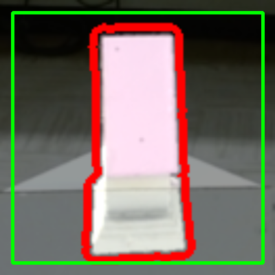
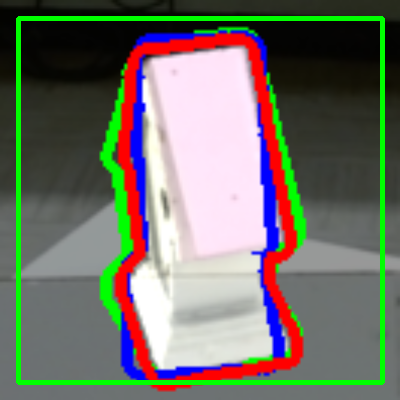
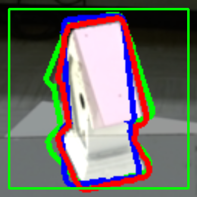
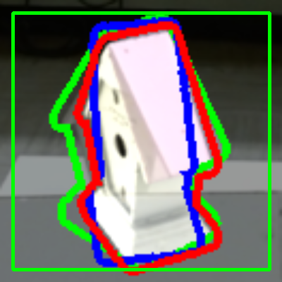
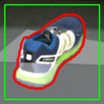
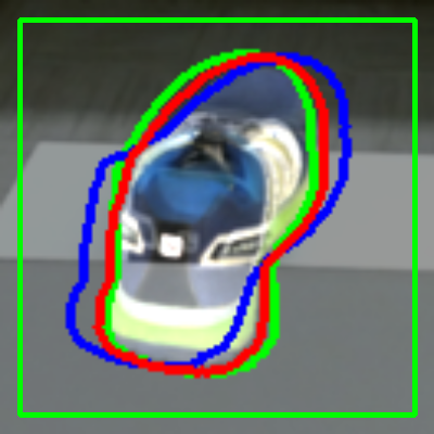
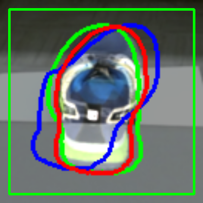
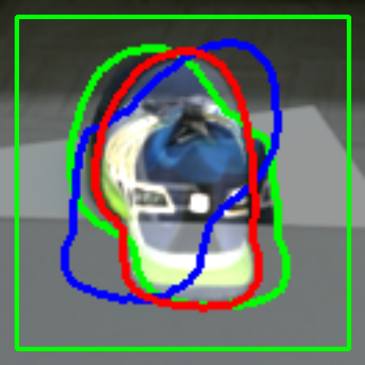
Figure 1: Given a 2D bounding box to select the object to track, our method recovers its 6D trajectory (3D translations and 3D rotations) for the next frames, without knowledge of the object geometry and without any training specific to the object. We use the ground truth 6D pose in the first frame and the 3D model for visualization only: The 3D model is rendered using 6D poses computed from the pose in the first frame and the trajectory we recover. For each row, the left image is the first frame of the sequence, which contains the given region of interest in green. The blue and red contours show the results of our two proposed methods, while the green contours delineate the ground truth object mask.

Recent methods such as LatentFusion [33], Gen6D [29], OnePose [41] address the problem of not having the 3D models for the target objects by first acquiring and registering reference images taken from multiple viewpoints. LatentFusion and OnePose also require a training phase. BundleTrack [53] does not require a 3D model a priori but relies on RGB-D images as input, which reveal the geometry of the object and thus simplify the problem. Therefore, being able to estimate the 6D pose of unkown objects from only RGB images remains an unsolved problem.

As shown in Fig. 1, in this paper, we demonstrate that it is possible to track the 6D pose of an object when no training images nor a 3D CAD model nor depth images are available for this object. Since we do not have access to the object’s 3D model nor its coordinate frame, only a relative pose up to a scale factor can be estimated. We therefore aim at predicting the 6D poses of unknown objects, not seen during training nor belonging to some specific category, relative to the first frame.

For our approach, which we call PIZZA for Powerful Image-only Zero-Shot Zero-CAD Approach, we rely on a Transformer encoder, which allows us to exploit an arbitrary number of past frames, in contrast with standard 3D tracking methods that typically rely on the previous frame only. Our Transformer-based method outputs the consecutive relative 6D poses between consecutive frames, which are then used recursively along with the initial object pose to provide the object 6D pose at each frame. As our experiments show, being able to exploit multiple frames reduces drift significantly compared to the standard frame-by-frame tracking framework.

One of the insights we had from our work is that the background has a strong influence on the accuracy of the predicted motions: In our early experiments, our motion prediction appeared to struggle on unseen objects over a cluttered background. This is in contrast with 6D pose prediction for seen objects, which can be made robust simply by training on images with cluttered background. However, training our method using similar complex backgrounds did not prove to be sufficient for unseen objects.

To alleviate the effect of complex background, we leverage recent progress in 2D unseen instance segmentation: We noticed that when trained on many examples, object segmentation networks generalize surprisingly well on unseen objects, even objects from unseen categories. We rely on the recent work [13] to get the objects’s masks in the input videos and discard the background. Even when the masks are noisy, this improves motion prediction significantly.

As mentioned above, the object motion can be retrieved only up to a scale factor. To guarantee the motion predictions are consistent across frames, special care is required: In particular, the magnitudes of the translations should be all defined up to the same scale factor. We propose a suitable representation of the motion at the beginning of Section 3.

We first validate our method on unseen categories with synthetic data created from CAD models of ModelNet [55] as done in [27, 42, 33] and synthetic videos created from CAD models of ShapeNet [9]. Then, we train our approach on a dataset made only of synthetic data created from rendering CAD models from BOP challenges [21] and test on real-world datasets Moped [33] and Laval [16]. We compare our methods with the state-of-the-art methods on deep 6D tracking methods: DeepIM [27], MultiPath Learning [42], LatentFusion [33], MoveIt [8] and Laval [16] which rely either 3D object models, or depth maps.

Thanks to domain randomization and realistic rendering, we achieve good generalization from synthetic to real data. Our method generalization capabilities are then two-fold, as it generalizes across domains, but also across novel object categories. We validate this by training only using synthetic data, and by making sure training and test objects belong to very dissimilar categories.

We believe our approach opens a new line of research on 6 DoF object tracking in open worlds, since to the best of our knowledge, it is the first method performing on RGB images that generalizes to unseen object categories without requiring any 3D information at train or test time such as depth maps or CAD models, nor pre-acquired reference images of the objects.

2 Related Work

In this section, we first give an overview of 6 DoF object pose estimation, from single-view estimation methods to tracking methods that use multiple images for inference. We then briefly discuss unseen object segmentation and 2D tracking, as this aspect is important in our approach.

2.1 6 DoF Object Pose Estimation

Monocular 6D pose estimation.

With the construction of various benchmarks for 6D object pose estimation [19, 20, 3, 4, 1], deep learning-based approaches have become dominant in this field. These methods can be roughly divided into three types of approaches: direct regression of the object pose [23, 56], template-based matching [19, 43] that encodes images in latent spaces and compares them against a dictionary of predefined viewpoints, and keypoint prediction for predicting the 6D pose [39, 48, 37, 22, 2] or dense 2D-3D correspondences [28, 51, 58, 34] as in earlier works [46, 7].

Most existing learning-based methods are designed for known objects; very few works report performances on unseen objects by using object descriptors [54, 6, 42], generic 2D-3D correspondences shared for all objects [38], or latent 3D representations [33]. Recently, Gen6D [29] and OnePose [41] proposed an extension of LatentFusion [33] with only RGB annotated reference images for unseen pose estimation. These methods still rely on a 3D model of the target object or on reference images of the object captured under multiple viewpoints; category-level methods can generalize to unseen objects of the known categories without knowing the exact 3D model [17, 51, 10, 31]. While Gen6D and OnePose do not require a 3D model of the object, they still require a sequence of images taken from different views of the target object as reference images. Capturing the reference images still require human expertise and some time for capture and registration.

Temporal 6D pose tracking.

Instead of relying on a single image for absolute pose estimation, tracking methods exploit temporal information. While earlier methods were prone to fail in the presence of heavy occlusion and clutter [25, 11, 5], data-driven methods have been proposed to learn more robust features by using Random Forests [24, 44, 45]. This problem has been recently formulated under a deep learning framework, where a network is trained to regress the pose difference between image pairs extracted from RGB [12, 8] or RGB-D videos [15, 16, 59, 50]. [16, 8, 53] show that this network can be applied to new objects but still require 3D information in the form of a CAD model or depth images.

In contrast to aforementioned deep 6D tracking methods that rely on either 3D object models, or depth maps, we introduce a generic RGB-based tracking method without 3D models, which can be trained on synthetic images only. To the best of our knowledge, we are the first to report object pose tracking performance on unseen objects, without using 3D object models or depth maps at test time.

2.2 2D Object Segmentation for Unseen Categories

Object segmentation methods first considered a “closed-world” setting, where the training and test sets share the same object classes. However, several authors, for example [14], noticed that a class-agnostic instance segmentation network is capable of generalizing to objects from unseen classes. The Unsupervised Video Objects (UVO) dataset was recently introduced by [52] to rigorously benchmark the performance of different methods for segmentation of unseen classes. In this work, we selected [13] to detect and segment the objects, because it is currently the best performing method on UVO. [13] relies on a two-stage network: The first stage consists of a class-agnostic object detector for proposal generation. The content in the proposals are fed to a foreground-background segmentation network to generate masks. This segmentation network relies on UPerNet [57] with Swin-L [30] as backbone. It extracts features at multiple scales to predict robust and accurate masks.

3 Our 6D Tracking Method

Given an image stream capturing a moving object and its 3D pose in the first frame, we want to predict the 6D pose of the pictured object in every frame. In this section, we first briefly describe the method we use for tracking and segmenting the target object in videos (Section 3.1): From the tracking part, we obtain 2D bounding boxes of the object, which we use to define the input to our network for motion prediction. The segmentation allows us to remove the background, as we noticed it has an adverse influence on motion prediction.

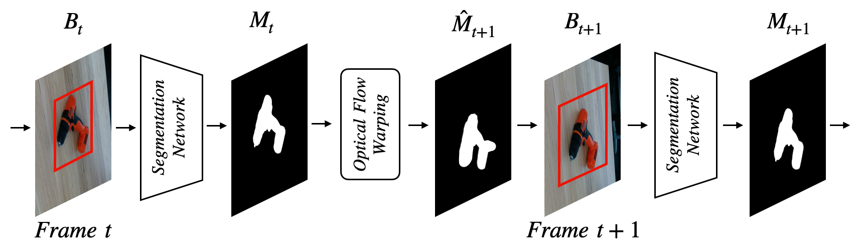
Figure 2: Tracking and segmenting the target object. Segmenting the object to discard background is important for good performance in complex scenes. From a 2D bounding box $B_{t}$ for the object at time $t$, we obtain its mask $M_{t}$ using a foreground-background segmentation network. We then use optical flow to predict a first estimate $\hat{M}_{t+1}$ of its mask in the next frame. From $\hat{M}_{t+1}$, we estimate its new bounding box $B_{t+1}$, on which we run the segmentation network to obtain a better mask $M_{t+1}$. This simple process is iterated over the sequence and was sufficient for our experiments.

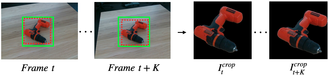
Figure 3: Left: We apply the same crop (in green) to the $K$ consecutive input images, which keeps the smallest box containing all extracted bounding boxes from $B_{t}$ to $B_{t+K}$ (in red). Right: the resulting images, after cropping and background masking.

Then, we describe the parameterizations for the 3D translation (Section 3.2) and for the 3D rotation (Section 3.3) that we propose for our problem. These parameterizations are important because they are adapted to the prediction of the 6D pose in our context, and our networks rely on them to predict the 6D poses. We then detail the architecture we use for multiple frame input (Section 3.4).

3.1 2D Unseen Object Tracking and Segmentation

We rely on a simple method for estimating 2D bounding boxes for the target object over an input video. We also obtain 2D masks for the object. A more sophisticated tracking method could be developed to prevent drift if it occurs, but it was sufficient for our experiments, thanks to the performance of the segmentation network from [13].

This method is illustrated in Fig. 2. We start from a given 2D bounding box $B_{0}$ for the object in the first frame: This bounding box indicates to the method which object should be tracked and segmented. [13] gives us the object mask $M_{0}$ in this bounding box.

By warping the mask $M_{0}$ using optical flow to the second frame, we obtain a prediction $\hat{M}_{1}$ for the object’ mask in the second frame. We use $\hat{M}_{1}$ to compute the bounding box $B_{1}$ for this frame. By applying [13] again to $B_{1}$, we obtain a better mask estimate $M_{1}$. We iterate this process to track the target object over the video. In practice, we use RAFT [47] to predict the optical flow.

As shown in Fig. 3, we feed our deep model with $K$ local frames to predict the object relative poses. These local frames are obtained by masking the background with masks $\hat{M}_{1}$ and applying the same cropping operation to all the frames we consider. This cropping operation returns the smallest image region that contains all the bounding boxes $\{B_{t}\}_{t}$ for the $K$ frames. In this way, the local frames are aligned together, which is important for the network to predict a consistent motion.

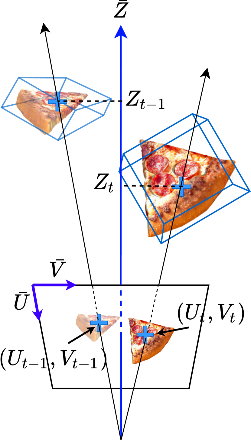
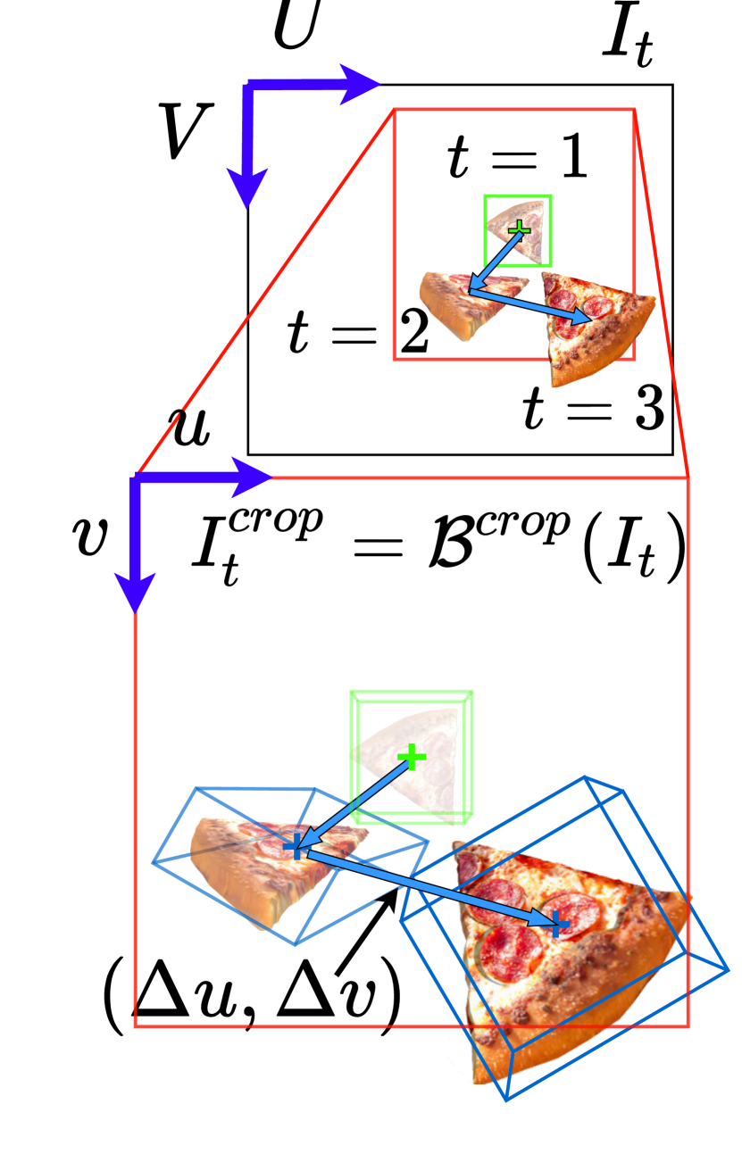
Figure 4: Estimating the 3D translation. Left: To predict the 3D object translation between two frames, we consider the 2D displacement of the projection of the object center and the scale change of its $Z$ coordinate. Right: The 2D displacement and the scale change are predicted from image regions extracted from the two frames image and need to be scaled.

3.2 Estimating the 3D Relative Translation

Fig. 4 provides an overview of our parameterization of the 3D relative translation and its estimation.

Parameterization of 3D Relative Translation.

The relative translation $\Delta{\bf T}_{t-1,t}\in{\mathds{R}}^{3}$ between two frames $I_{t-1}$ and $I_{t}$ can be expressed as $\Delta{\bf T}_{t-1,t}={\bf T}_{t}-{\bf T}_{t-1}$, where ${\bf T}_{t}$ is the 3D object center in the camera coordinate system for frame $I_{t}$. In our case, we do not have access to the actual 3D size of the object, and we cannot directly estimate the norm of the relative translation $\Delta{\bf T}_{t-1,t}$. To introduce our translation parametrization, let’s us first rewrite $\Delta{\bf T}_{t-1,t}$ as:

$$\Delta{\bf T}_{t-1,t} ={\bf T}_{t}-{\bf T}_{t-1}$$ (1)

$$=Z_{t}\text{K}^{-1}\begin{bmatrix}U_{t}\\ V_{t}\\ 1\end{bmatrix}-Z_{t-1}\text{K}^{-1}\begin{bmatrix}U_{t-1}\\ V_{t-1}\\ 1\end{bmatrix}\>,$$

where $(U_{t},V_{t})$ are the pixel coordinates of the object’s center reprojection and $Z_{t}$ its depth for frame $I_{t}$. $\mathrm{K}$ is the camera intrinsic matrix. During tracking on frame $I_{t}$, we have already estimated $(U_{t-1},V_{t-1})$ and it is simpler to predict the 2D displacement $(\Delta U_{t-1,t},\Delta V_{t-1,t})$ of the object center between previous frame $I_{t-1}$ and current frame $I_{t}$:

$$\Delta U_{t-1,t}=U_{t}-U_{t-1}\text{ and }\Delta V_{t-1,t}=V_{t}-V_{t-1}.$$ (2)

Moreover, estimating the absolute depth value $Z_{t}$ or absolute depth variation $\Delta Z_{t-1,t}$ is also not possible in our case, we also introduce the normalized depth offset $S_{t-1,t}$ in log-scale as:

$$S_{t-1,t}=\frac{Z_{t}}{Z_{t-1}}-1\>.$$ (3)

Note that in practice, $S_{t-1,t}$ varies around 0.

In practice, it is important to restrict the input images to a window more or less centered on the object for pose prediction: This cropping operation removes most of the background, which is irrelevant and a nuisance to pose estimation. It has however an influence on our translation parameterization. Indeed, the cropped regions have to be scaled to use them as input to our network, which expect images of fixed resolution. The network predicts a 2D displacement $(\Delta u,\Delta v)$ in the scaled cropped regions, and the original displacement in the image frame can be retrieved by:

$$\Delta U=\alpha_{u}\mathrm{W}^{\text{crop}}\Delta u\quad\textrm{and}\quad\Delta V=\alpha_{v}\mathrm{H}^{\text{crop}}\Delta v\>,$$ (4)

where $\alpha_{v}$ and $\alpha_{v}$ are the scale factors along the $u$ and $v$ axes of the images between the cropped regions and the network inputs. The network also predicts a depth offset $s$ for the scaled cropped regions, which also needs to be rescaled, and we use:

$$S=\frac{\alpha_{u}+\alpha_{v}}{2}s\>.$$ (5)

Recovering $\Delta{\bf T}_{t-1,t}$ and ${\bf T}_{t}$.

If ${\bf T}_{t-1}$ is known, we can estimate $\Delta{\bf T}_{t-1,t}$ and ${\bf T}_{t}$ from $\Delta U$, $\Delta V$, and $S$. In our experiments, and only when comparing with previous works, we assume that the location ${\bf T}_{1}$ of the object in the first frame is known in metric values, so that we can also recover the object trajectory in metric values. In our actual scenario, when no metric information is available, $Z_{1}$ can be set to an arbitrary positive value, and the object trajectory will be recovered up to this scale factor.

Given a frame $I_{t}$, together with the object center $(U_{t-1},V_{t-1})$ in the previous frame $I_{t-1}$, we first predict $(\Delta u_{t-1,t},\Delta v_{t-1,t},s_{t-1,1})$ from the cropped images $I^{\text{crop}}_{t-1}$ and $I^{\text{crop}}_{t}$. Then, after conversion from local coordinates to pixel coordinates using Eq. (4), we obtain the object center $(U_{t},V_{t})$ from Eq. (2), and depth value $Z_{t}$ from Eq. (3). We finally retrieve the 3D translation vector between the object poses in the two frames with Eq. (1).

Translation Loss.

The 3D translation of the target object between two frames is parameterized as a 2D displacement $(\Delta u,\Delta v)$ expressed in the cropped region frames and the depth scaling factor $s$. The training loss is implemented as:

$${\cal L}_{\Delta{\bf T}}=\ell_{1}(\Delta u,\Delta u^{*})+\ell_{1}(\Delta v,\Delta v^{*})+\lambda\ell_{1}(s,s^{*})\>,$$ (6)

where $\Delta u^{*}$, $\Delta v^{*}$, and $s^{*}$ are ground truth values, $\ell_{1}$ is the smooth-L1 loss, and weight $\lambda$ is set to 1 in practice.

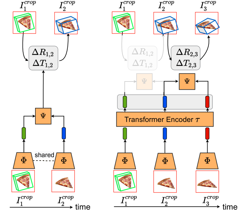
Figure 5: The two architectures we consider: Our baseline two-frame architecture is a simple CNN-based architecture that predicts the 3D motion between two frames from these two frames only (left); Our multi-frame architecture relies on a Transformer encoder to exploit efficiently more frames as input (right). It accepts an arbitrary number of past frames as input to predict the 3D motion between the previous and current frames. All learnable components (in orange) are trained end-to-end.

3.3 Estimating the 3D Relative Rotation

Parameterization of the 3D rotation.

The relative rotation is much simpler to handle than the relative translation as it does not depend on the actual size of the object nor the scaling of the images used as input to the network. The relative rotation $\Delta{\bf R}_{t-1,t}\in SO(3)$ between $I_{t-1}$ and $I_{t}$ is defined as:

$$\Delta{\bf R}_{t-1,t}={\bf R}_{t}{\bf R}_{t-1}^{\top}\>,$$ (7)

where ${\bf R}_{t}$ is the 3D object rotation in the camera coordinate system. The rotation ${\bf R}$ can be parameterized in different ways. After conducting a thorough comparative study, we opted for the axis-angle representation. This representation is defined by a vector $\boldsymbol{\omega}\in{\mathds{R}}^{3}$, where $\|\boldsymbol{\omega}\|$ and $\boldsymbol{\omega}/\|\boldsymbol{\omega}\|$ define the rotation angle and axis, respectively. More details can be found in the supplementary material.

Rotation Loss.

We train our networks using a simple L2 loss on the axis-angle representation:

$${\cal L}_{\boldsymbol{\omega}}=\|\boldsymbol{\omega}-\boldsymbol{\omega}^{*}\|^{2}\>,$$ (8)

where $\boldsymbol{\omega}^{*}$ denotes the ground truth axis-angle.

Recovering ${\bf R}_{t}$.

If ${\bf R}_{t-1}$ is known, we can recover ${\bf R}_{t}$ once we estimated $\Delta{\bf R}_{t-1,t}$. In our experiments, for comparison with other works, we will assume that the initial rotation ${\bf R}_{1}$ is known for the first frame of the trajectory. This is however only for comparison purposes. In our scenario, when no 3D model is available to define a coordinate frame, the rotation for the first frame can be set to an arbitrary rotation, for example the Identity matrix. The object trajectory will be recovered up to this rotation.

Result: $\{({\bf R}_{i},{\bf T}_{i}),\textrm{for all images }I_{i}\textrm{ in }\mathcal{S}\}$

Input :  Input image sequence $\mathcal{S}=\{I_{1},...,I_{N}\}$;

Object initial 2D center $(U_{1},V_{1})$;

Object initial rotation ${\bf R}_{1}$;

Object initial depth $Z_{1}$;

for ( $t\in[2;N[$ ) $\{$

      

      $[\mathbf{f}_{1},...,\mathbf{f}_{n}]=[\Phi(I_{1}),...,\Phi(I_{n})]$;

       if Multiple Frames with Transformer $\mathcal{T}$ then

             $[\mathbf{f}_{1},...,\mathbf{f}_{n}]\leftarrow\mathcal{T}(\mathbf{f}_{1},...,\mathbf{f}_{n})$ // Eq.(9)

            

       end if

      // See Sec.3.2 and Sec.3.3

       $(\boldsymbol{\omega},\Delta u,\Delta v,s)=\Psi(\mathbf{f}_{t-1},\mathbf{f}_{t})$// Eq.(10)

       ${\bf T}_{t-1}=Z_{t-1}\text{K}^{-1}[U_{t-1},V_{t-1},1]^{T}$;

       $\Delta U,\Delta V\leftarrow$// Use Eq.(4)

       $U_{t},V_{t}\leftarrow$// Use Eq.(2)

       $Z_{t}\leftarrow$// Use Eq.(3)

       $\Delta{\bf T}\leftarrow$// Use Eq.(1)

       $\Delta{\bf R}\leftarrow$// Use Rodrigues Formula on $\boldsymbol{\omega}_{\Delta{\bf R}}$

       ${\bf R}_{t}\leftarrow(\Delta{\bf R}){\bf R}_{t-1}$;

       ${\bf T}_{t}\leftarrow{\bf T}_{t-1}+\Delta{\bf T}$;

      

$\}$

Algorithm 1 Computing the object trajectory for a given image sequence $\mathcal{S}$ with our Transformer-based architecture. The object center $(U_{1},V_{1})$ is provided by the user. The initial rotation can be initialized to the identity, and $Z_{1}$ to an arbitrary positive value. For the purpose of comparison with previous work, we initialize them to ground truth value as they do.

3.4 Proposed Architecture

In order to efficiently incorporate information across multiple frames, and as illustrated in Fig. 5, our architecture takes a sequence of frames as input to predict the relative pose between the two last frames. It first converts frames $\{I_{t-N},\dots,I_{t}\}$ into a set of image features $\{\mathbf{f}_{t-i}=\Phi(I_{t-i}),i=1..N\}$ using an image embedding module $\Phi$ implemented as a ResNet18. It then projects these image features into another embedding space where interframe correlation is enhanced by the self-attention mechanism of the Transformer encoder $\mathcal{T}$:

$$\{\mathbf{f}_{t-N},\dots,\mathbf{f}_{t}\}\leftarrow\mathcal{T}\big{(}\mathbf{f}_{t-N}\dots\mathbf{f}_{t}\big{)}\>.$$ (9)

We then predict the relative pose between $I_{t-1}$ and $I_{t}$ using

$$(\boldsymbol{\omega}_{{t-1,t}},\Delta u_{t-1,t},\Delta v_{t-1,t},s_{t-1,t})=\Psi(\mathbf{f}_{t-1},\mathbf{f}_{t})\>,$$ (10)

where the pose regressor $\Psi(\cdot)$ is implemented as two 3-layer MLPs $\Psi_{\bf R}$ and $\Psi_{\bf T}$, respectively for rotation and translation estimation. We detail the architecture of these MLPs in the supplementary material. We train the different modules jointly in an end-to-end fashion.

We also consider a baseline that takes information extracted from only two input frames and which relies on a more standard deep architecture. As our experiments will show, the Transformer-based architecture achieves significantly better performances compared to this baseline.

6D Tracking in sequences.

Finally, our 6D tracking algorithm, which we summarize in Algorithm 1, returns a sequence of 6D poses by chaining relative poses predicted from consecutive frames.

4 Experiments

We conduct extensive experiments to evaluate the generalization capabilities of our method to unseen categories. We compare with CAD-based methods: DeepIM [27], MultiPath Learning [42], MoveIt [8], and to RGB-D based methods: LatentFusion [33] and Laval [16]. The latter uses both CAD and RGB-D images. LatentFusion requires not only the depth maps but also reference images to obtain 3D features before pose estimation. The main characteristics of all synthetic and real-world datasets we consider are summarized in Table 1.

We provide here qualitative examples, but much more results can also be found in the supplementary material.

Domain	Name	#Training images	#Test images	Videos
Synthetic	ModelNet	420’400	35’000
	ShapeNet	400’000	100’000	✓
Real-world	BOP	22’500	0	✓
	Laval	0	14’190	✓
	Moped	0	3’079	✓

Table 1: Characteristics of the datasets considered in this paper.

4.1 Experimental Setup

	(5$\circ$, 5cm)				ADD (0.1d)				Proj2D (5px)
Methods	DeepIM	MP	Latent	Ours 2F	DeepIM	MP	Latent	Ours 2F	DeepIM	MP	Latent	Ours 2F
CAD	✓	✓			✓	✓			✓	✓
Depth			✓				✓				✓
bathtub	71.6	85.5	85.0	50.0	88.6	91.5	92.7	83.6	73.4	80.6	94.9	52.3
bookshelf	39.2	81.9	80.2	68.3	76.4	85.1	91.5	79.4	88.3	76.3	91.8	70.0
guitar	50.4	69.2	73.5	31.2	69.6	80.5	83.9	63.7	77.1	80.1	96.9	67.2
range_hood	69.8	91.0	82.9	60.3	89.6	95.0	97.9	90.9	70.6	83.9	91.7	46.9
sofa	82.7	91.3	89.9	77.6	89.5	95.8	99.7	92.9	94.2	86.5	97.6	78.6
tv_stand	73.6	85.9	88.6	83.2	92.1	90.9	97.4	95.3	76.6	82.5	96.0	85.8
wardrobe	62.7	88.7	91.7	92.0	79.4	92.1	97.0	98.0	70.0	81.1	94.2	85.8
Mean	64.3	84.8	85.5	66.1	83.6	90.1	94.3	87.5	73.3	81.6	94.7	69.5

Table 2: Comparison to DeepIM [27], Multi-Path Learning (MP) [42] and LatentFusion (Latent) [33] on unseen categories of the ModelNet dataset. Note that DeepIM and MP require the CAD models for refinement; LatentFusion uses RGB-D images and reference frames. In all cases only two consecutive frames are used, which is why we only report results for our two-frame method.

4.1.1 Synthetic Datasets

We follow previous works [33] to generate a synthetic dataset from CAD models of ModelNet [55]. The target view is rendered at constant translation $t=(0,0,500\leavevmode\nobreak\ mm)$ and random rotation $R$. Then, we render another view with that pose perturbed by angles $\beta_{\{x|y|z\}}\sim\mathcal{N}(0,\,(15^{o})^{2})$ for each rotation axis and a translational offset $(\Delta x,\Delta y,\Delta z)$ with $\Delta_{\{x|y\}}\sim\mathcal{N}(0,10^{2})$, $\Delta z\sim\mathcal{N}(0,50^{2})$ (mm) with the total angular perturbation lower than $45^{o}$.

Previous methods only evaluate their models with pairs of images, we generalize this setting to multi-frames with CAD models from ShapeNet to evaluate the performance of the methods on long sequences. To do so, we create new synthetic videos by following [16]: the first frame of the video is rendered with a random translation $t=(0,0,Z)$ (mm) with Z sampled uniformly from 0.4m to 2m and a random rotation $R\sim SO(3)$. The next frame is rendered by perturbating the object pose in the previous frame by angles $\beta_{\{x|y|z\}}\sim\mathcal{N}(0,\,(20^{o})^{2})$ and a translation$\Delta_{\{x|y|z\}}\sim\mathcal{N}(0,20^{2})$ (mm). We iterate the process until we get 100 frames for each CAD model. More detailed about synthetic data generation can be found in the supplementary material.

4.1.2 Real-world Datasets

In addition to the synthetic datasets, we evaluate our methods on two different real-world datasets: 1) the Laval dataset [16], which contains 297 sequences of 11 real objects captured in 3 different scenarios. As the interaction scenario of Laval [16] requires hand occlusion which is a very specific setting, we follow MoveIt [8] by focusing more on the occlusion scenario. Note that MoveIt only evaluates on 8 of the 11 objects of Laval, while we evaluate on all 11 objects and report the averaged performance; 2) the MOPED dataset [33], which consists of 11 household objects covering all views of the objects.

4.1.3 Implementation Details

We implemented our models using the Pytorch [36] framework. The image encoding module $\Phi$ is a ResNet18 [18] which extracts a global embedding of dimension 256 for each input image resized to $224\times 224$. The pose regressor $\Psi$ is composed of two identical MLPs with three hidden layers of size 800-400-200. The Transformer encoder $\mathcal{T}$ is implemented with a single multi-head self-attention layer with 12 heads, and 512 hidden neurons in the feedforward (MLP) layer. More details are given in the supplementary material.

		Bathtub	Bookshelf	Bus	Car	Cabinet	Display	Telephone	Mean
Translation (mm)	Avg signed motion	24.1	24.1	24.5	23.8	24.7	23.9	25.3	24.3
	Ours 2F	14.1	14.9	14.3	13.6	13.4	15.27	15.3	16.2
	Ours MF	13.1	13.8	13.1	11.8	12.8	14.2	13.6	13.2
Rotation (deg)	Avg signed motion	20.8	20.5	20.8	20.7	20.6	21.0	21.0	20.7
	Ours 2F	5.4	5.2	5.4	3.8	5.6	6.3	5.7	5.3
	Ours MF	5.4	4.8	4.8	3.3	4.5	5.9	5.6	4.9

Table 3: Comparaison of our two-frame (Ours 2F) and our multi-frames (Ours MF) architectures on synthetic videos of ShapeNet. “Average signed motion” gives the average motion over all the sequences of 15 frames in our synthetic videos. Ours MF outperforms Ours 2F on all the categories.

4.1.4 Evaluation Metrics

We use five evaluation metrics as done in [27, 42, 33, 8, 16]: 1) $(k^{\circ},k\leavevmode\nobreak\ \text{cm})$: a pose is considered correct if the geodesic error and translation error are within $k^{\circ}$ and $k$ cm. 2) ADD [19]: the average distance between points after being transformed by the ground truth and predicted poses. 3) ADD-S: a modification to ADD that computes the average distance to the closest point rather than the ground truth point to account for symmetric objects. 4) Proj.2D: the pixel distance between the projected points of the ground truth and predicted pose. 5) the geodesic error and translation error between the prediction and the ground-truth for every sequence of 15 frames as done in [16, 8].

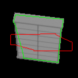
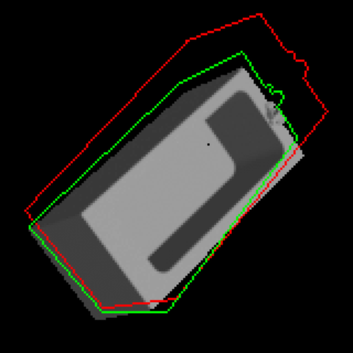
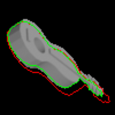
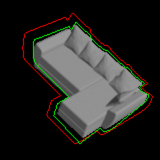
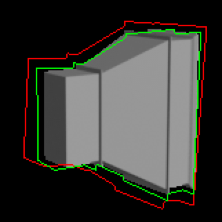
Figure 6: Qualitative results on ModelNet. We show the target image with an initial perturbed pose in a red wireframe and our pose prediction with a green wireframes. The object wireframes are used only for visualization.

Method	CAD	Depth	Translation (mm)				Rotation (deg)
			Occlusion				Occlusion
			$0\%$	$15\%$	$30\%$	$45\%$	$0\%$	$15\%$	$30\%$	$45\%$
Laval  [16]	✓	✓	6.7	11.1	18.9	25.9	5.3	8.4	16.1	26.8
MoveIt [8]	✓		14.5	13.9	25.1	22.5	33.3	31.8	34.1	28.86
Ours 2F			16.18	14.92	15.38	15.44	19.83	20.78	20.16	20.33
Ours MF			9.82	10.27	9.97	10.16	16.41	16.13	16.21	17.76

Table 4: Comparison with 3D tracking methods Laval generic [16] and MoveIt [8] on the Laval dataset. Laval generic uses the object’s 3D model and depth maps; MoveIt uses the 3D model. We use neither of these extra inputs. Our method is more robust to occlusion compared to other methods and achieves better superior performance on videos with severe occlusion.

4.2 Evaluation on Synthetic Datasets

4.2.1 Results on ModelNet

We compare the performance of our method with DeepIM [27], MultiPath Learning (MP) [42] and LatentFusion [33] on the unseen classes of ModelNet [55]. Both DeepIM and MP require the object’s CAD model for prediction while LatentFusion relies on depth images during testing. Our method takes only RGB images as input during testing. As shown in Table 2, our method can achieve comparable performance for the ADD metric while requiring much less information. Our method even achieves better results than DeepIM for the $(5^{\circ},5cm)$ and ADD metrics. Furthermore, our method estimates directly the relative pose without any iterative refinement adopted in DeepIM and MP, which demonstrates the effectiveness of our method on unseen classes. We show the output of our method on the ModelNet dataset in Fig. 12.

4.2.2 Results on ShapeNet

We compare the performance of our two-frame architecture network which takes two frames as input with our multi-frame Transformer based network in the ShapeNet setting. As shown in Table 3, our multi-frame Transformer outperforms the two-frame architecture network on every unseen class, which validates the benefit of taking multiple frames as input and demonstrates the effectiveness of our multi-frame Transformer network.

4.3 Evaluation on Real-World Datasets

4.3.1 Results on Laval

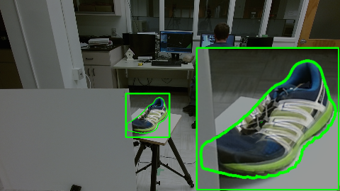
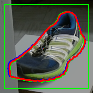
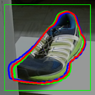
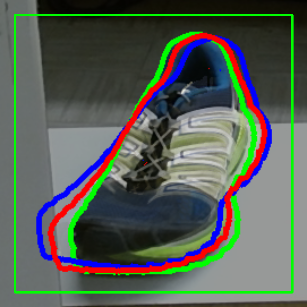
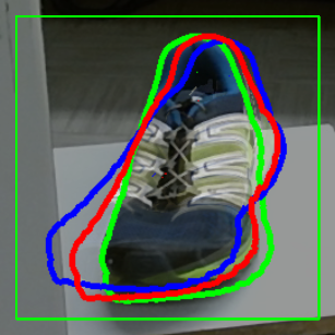
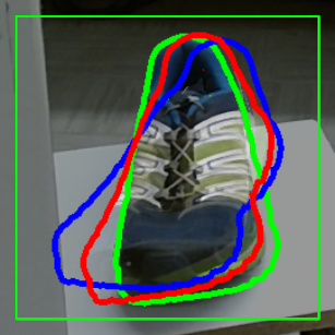
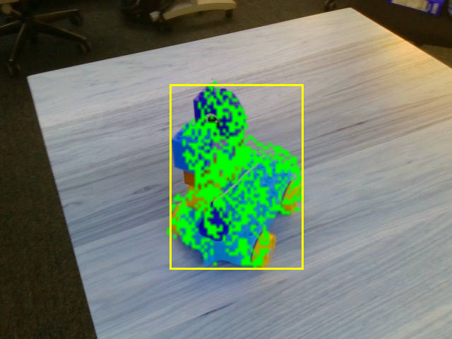
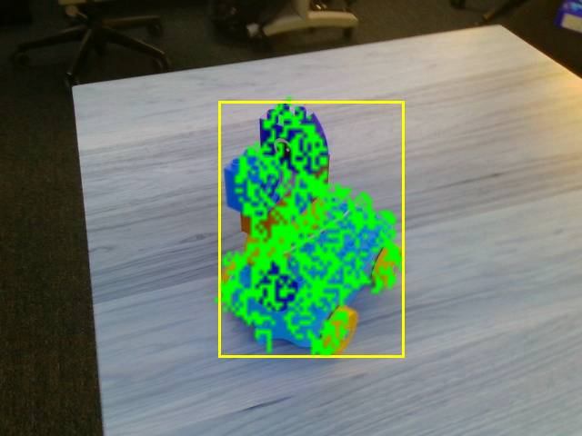
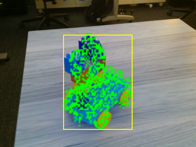
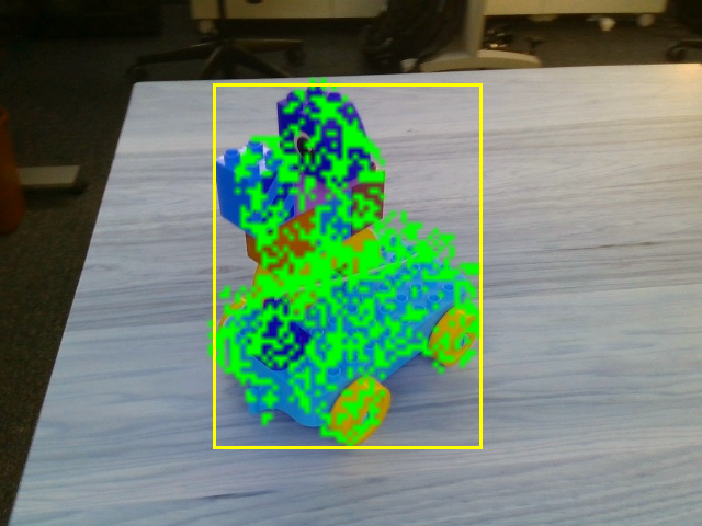
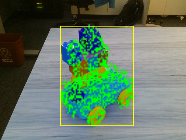
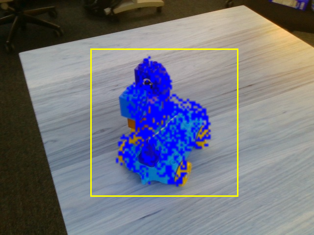
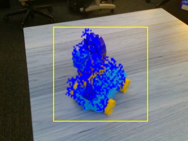
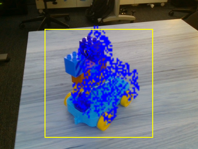
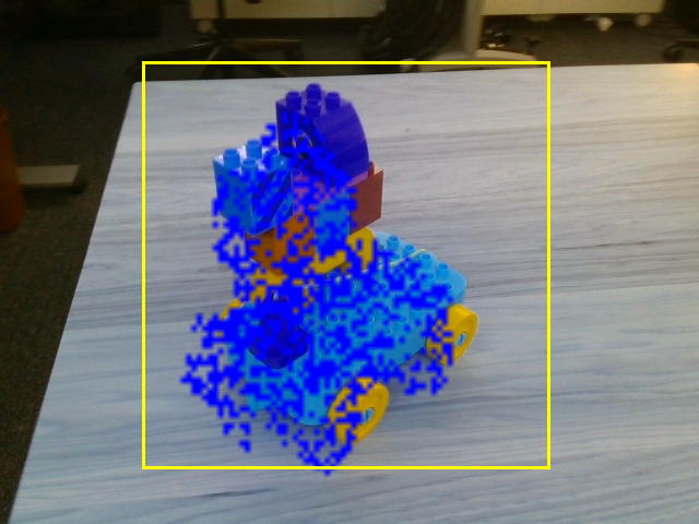
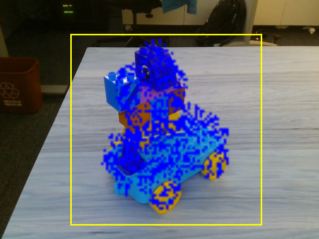
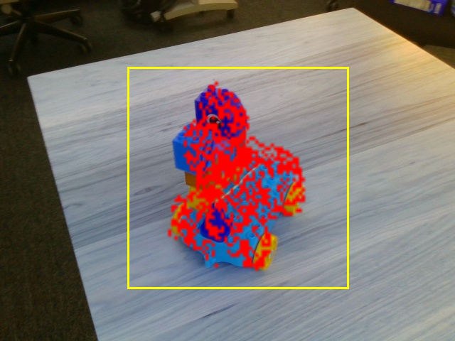
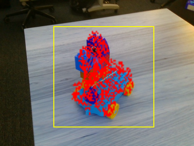
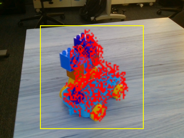
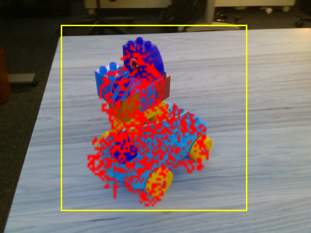
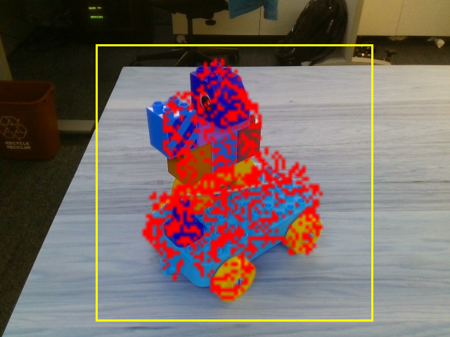
Figure 7: Qualitative results on real-world datasets. We show in each image the ground-truth in green, the prediction with Ours two-frame in blue and the prediction with Ours multi-frame in red. First row shows our results on a sequence images of object “shoe” of the Laval dataset [16]. The three last rows show our results on a sequence of images on Object “duplo_dude” of the Moped dataset [33].

We compare our method with two recent methods: Laval-generic [16] and MoveIt [8]. Following their evaluation protocol, the ground truth pose is given every 15 frames. Table 4 reports the results. Our two-frame architecture network is comparable to other methods without using the CAD models or depth images. Our multi-frame Transformer network further boosts the performance. Our method achieves superior results especially on sequences with severe occlusion, and our method degrades very little compared with other methods when increasing the occlusion rate. Thus, our method is more robust to occlusion. Our two models, especially the multi-frame version, achieve very good results and even often outperform the two other methods despite a clear disadvantage. The multi-frame version achieves the best overall performance on 3D relative translation, and much better results for 3D relative rotation estimation than MoveIt that uses CAD models. Fig. 7 provides some qualitative results.

4.3.2 Results on Moped

We also compare our methods with LatentFusion [33], which relies on RGB-D images, on the Moped dataset. The performance of our method is comparable with LatentFusion when LatentFusion uses 1 reference image. It still has a 20% gap with LatentFusion, when LatentFusion uses 8 reference images. We show some outputs of our method on the Moped dataset in Fig. 7.

4.4 Limitations

	AUC (ADD)$\uparrow$				AUC (ADD-S)$\uparrow$
Methods	Latent	Latent	Ours 2F	Ours MF	Latent	Latent	Ours 2F	Ours MF
Depth	✓	✓			✓	✓
# R. views	1	8	1	1	1	8	1	1
black_drill	-	89.4	44.6	45.6	-	95.1	62.4	68.9
cheezit	-	24.6	44.9	42.0	-	92.2	72.4	74.4
duplo_dude	-	88.9	38.4	39.1	-	94.7	62.7	69.7
duster	-	47.2	55.0	57.2	-	87.9	78.5	84.3
graphic_card	-	73.0	45.5	47.9	-	79.2	70.3	77.7
orange_drill	-	78.3	49.1	52.2	-	93.5	64.7	72.7
pouch	-	54.8	26.7	23.9	-	91.7	41.5	42.8
remote	-	60.0	64.1	64.4	-	91.9	73.9	79.8
rinse_aid	-	67.4	70.2	72.0	-	93.3	83.2	90.7
toy_plane	-	82.9	21.4	22.3	-	92.2	43.9	50.1
vim_mug	-	40.0	61.9	60.4	-	91.7	79.0	83.5
Mean	23.9	68.3	47.5	47.9	78.7	90.9	66.6	72.2

Table 5: Comparison to LatentFusion (Latent) [33] on the Moped dataset. We report the Area Under Curve (AUC) for each metric as done in [33]. Note that our method does not require any reference image. Our method is comparable with LatentFusion when LatentFusion uses one reference image.

Our method comes with some limitations:

• Estimation of $\Delta T_{z}$: We show in the supplementary material that the translation error along the $Z$ axis is much larger than the errors along the other two axes. This is a common problem in 6D pose estimation: Estimating motion along the $Z$ axis is very challenging for RGB-based methods, as relatively large $\Delta T_{z}$ can occur even with minimal appearance change between two frames.

• Our method may fail when our segmentation model fails to segment the target object. However, our experience is that this model is surprisingly robust, and that our pose estimation model is robust to incorrect segments.

5 Conclusion

In this paper, we explored what can be done for 3D object tracking in the absence of 3D model, depth data, registered images, and even knowledge about the object class. The accuracy we obtain is surprisingly good, as it is on par with previous methods that have access to much more information. Beyond downstream possible applications such as robotics and Man-Machine-Interaction, we hope our approach will encourage more research on the “Zero-shot Zero-CAD” topic.

Acknowledgments. We thank Xi Shen and Mathis Petrovich for helpful discussions. This research was produced within the framework of Energy4Climate Interdisciplinary Center (E4C) of IP Paris and Ecole des Ponts ParisTech, and was supported by the 3rd Programme d’Investissements d’Avenir [ANR-18-EUR-0006-02], the support of the Chair “Challenging Technology for Responsible Energy” led by l’X – Ecole polytechnique and the Fondation de l’Ecole polytechnique, sponsored by TOTAL, and the ChistEra IPALM project. This work was performed using HPC resources from GENCI–IDRIS 2021-AD011012294.

Supplementary Material

6 Rotation representation

Figure 8 shows our ablation study on different representations of rotation on synthetic images created from CAD models of ShapeNet [9]: Euler angles, axis-angles, a quaternion and the rotation 6D method from [2]. While the rotation 6D method has been shown recently to be better than the other representations in absolute pose estimation [26], our ablation study shows that we do not gain the performance when the motion is small such as in objet tracking.

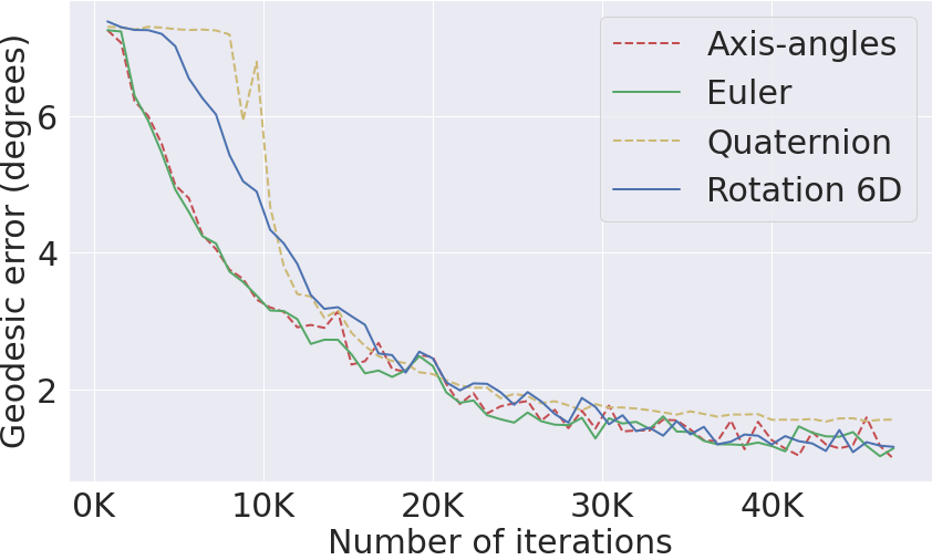
Figure 8: Ablation study on synthetic images created from CAD models of ShapeNet [9] with Our two-frames. The average of the rotational motion equal to 7.25 degrees. We show that the performance is almost the same when using different types of representation for the rotation.

7 Architecture details

Transformer.

Our Transformer $\mathcal{T}$ is implemented with the TransformerEncoder layer of Pytorch [36] with only one encoder layer with 12 heads and an MLP containing 512 hidden neurons. We do not use dropout in the encoder layer.

Pose Regressor.

Our pose regression module $\Psi(\cdot)$ is composed of two MLPs, one for translation and one for rotation. Each MLP is made of three layers with 800, 400, 200 hidden neurons respectively. The middle layers are followed by a batch normalization and a ReLU activation.

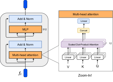
Figure 9: Architecture of our Transformer Encoder $\mathcal{T}$.

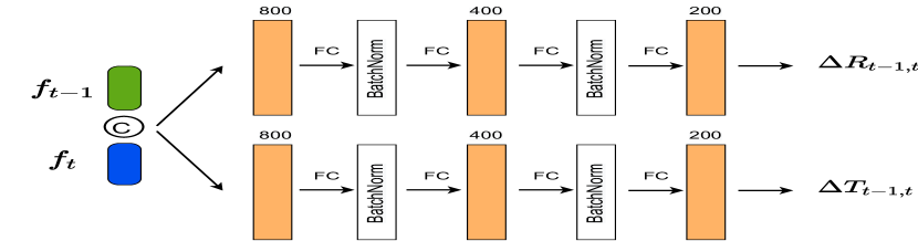
Figure 10: Architecture of our Pose Regressor $\Psi$. Given two global features $\mathbf{f}_{t-1}$ and $\mathbf{f}_{t}$ at the output of $\Phi$ in Our two-frame or of $\mathcal{T}$ in Our multi-frame, we concatenate them and predict relative pose change $\Delta{\bf R}_{t-1,t}$ and $\Delta{\bf T}_{t-1,t}$

8 Additional results

8.1 Evaluation on Synthetic Datasets

Mitigating Error Accumulation.

Tracking methods are prone to drift with time since they can accumulate of errors between each pair of consecutive frames. Figure 11 shows the average of rotation and translation errors over time on the test set of our ShapeNet dataset. As can be seen from the graphs, the multi-frame Transformer-based architecture. accumulates significantly less errors, making it a good candidate for tracking applications.

Tracking translation in Z axis.

As discussed in Section 4.3 of the main paper, most translation errors come from the Z camera axis for both methods when the tracking duration is small. This is because estimating motion along this axis is notoriously very challenging for RGB-based methods, as relatively large $\Delta T_{z}$ can occur even with minimal appearance change between two frames.

We show additional qualitative results on the ModelNet dataset in Figure 12.

8.2 Evaluation on Real-world Datasets

Failure cases of unseen object segmentation.

We show in Figure 13 some failure cases of the segmentation model [13] on unseen objects of Laval [16] and Moped [33].

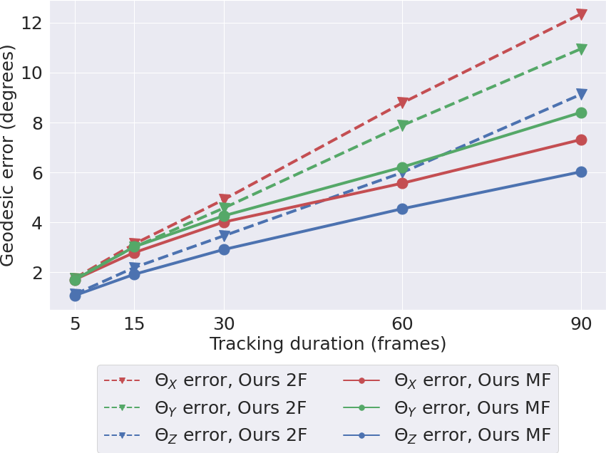
Figure 11: Error accumulation over time for our two architectures. Left: Rotation error over the 3 axes measured with Euler angles $(\theta_{X},\theta_{Y},\theta_{Z})$; Right: Translation error over the 3 axes. Interestingly, the translation error along the X and Y axes increases much slower with the multi-frame architecture than with the two-frame architecture.

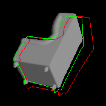
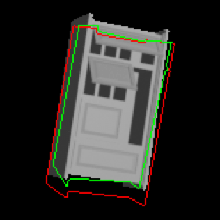
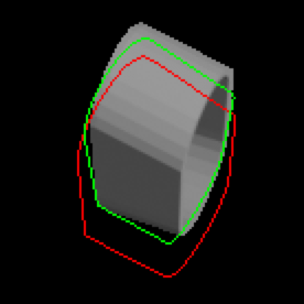
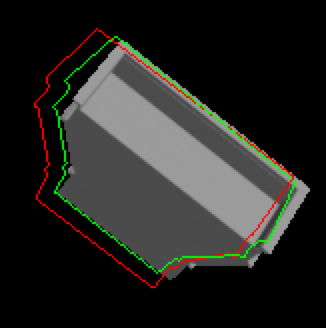
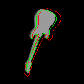
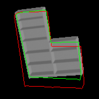
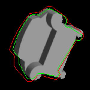
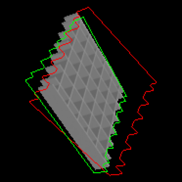
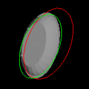
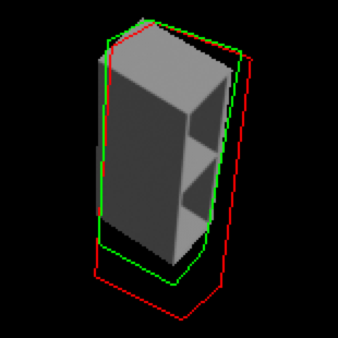
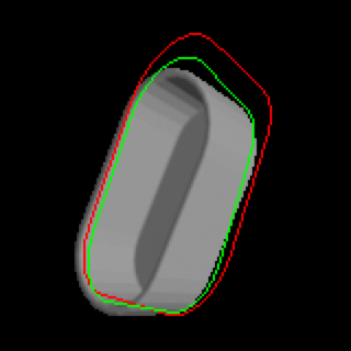
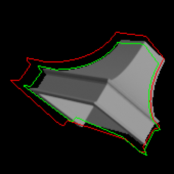
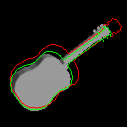
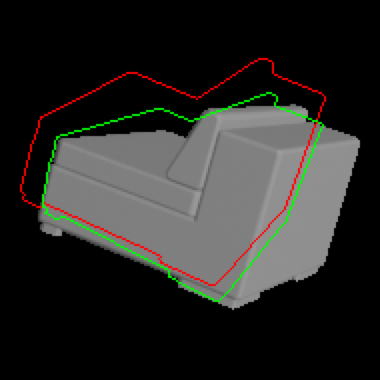
Figure 12: Qualitative results on ModelNet. We show the target image with an initial perturbed pose in a red wireframe and our pose prediction with a green wireframes. The object wireframes are used only for visualization.

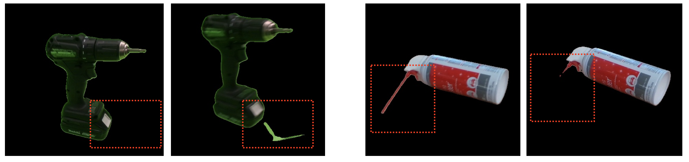
Figure 13: Failure case of segmentation model [13] in the highlight region in red color which creates “motion ambiguities” as the appearance changes are explained by other motions than correct ones.

Training objects from BOP [21].

We train our approach on a dataset made only of synthetic data created from rendering CAD models from BOP challenges [21] including: LINEMOD [19], HB [3], HOPE, RU-APC [4] datasets with BlenderProc [1]. We visually compare the training and testing objects in Figure 14.

We show additional qualitative results on Moped [33] and Laval [16] datasets in Figure 15 and Figure 16.

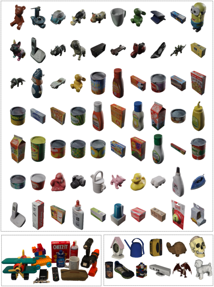
Figure 14: Visual comparison between training objects from BOP challenges [21] (top) and testing objects of Moped [33] (bottom left) and Laval [16] datasets (bottom right). The bottom images are taken from [33, 16].

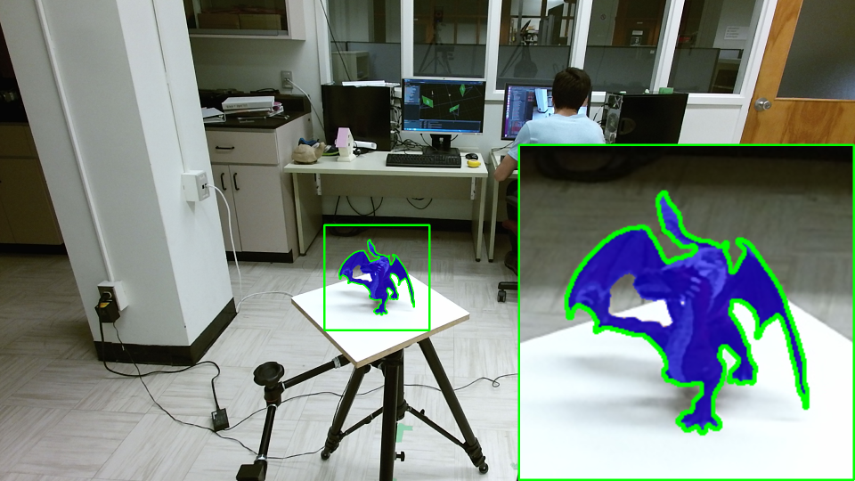
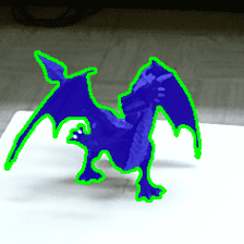
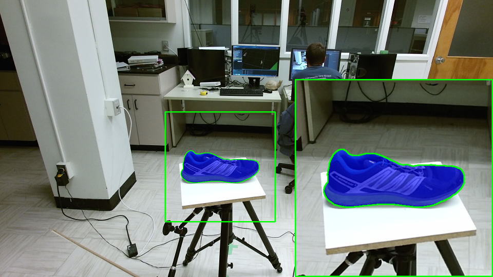
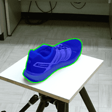
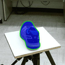
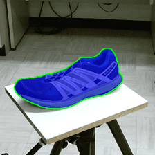
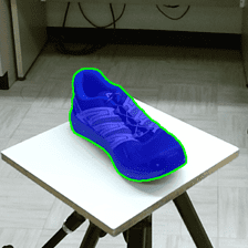
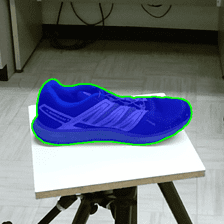
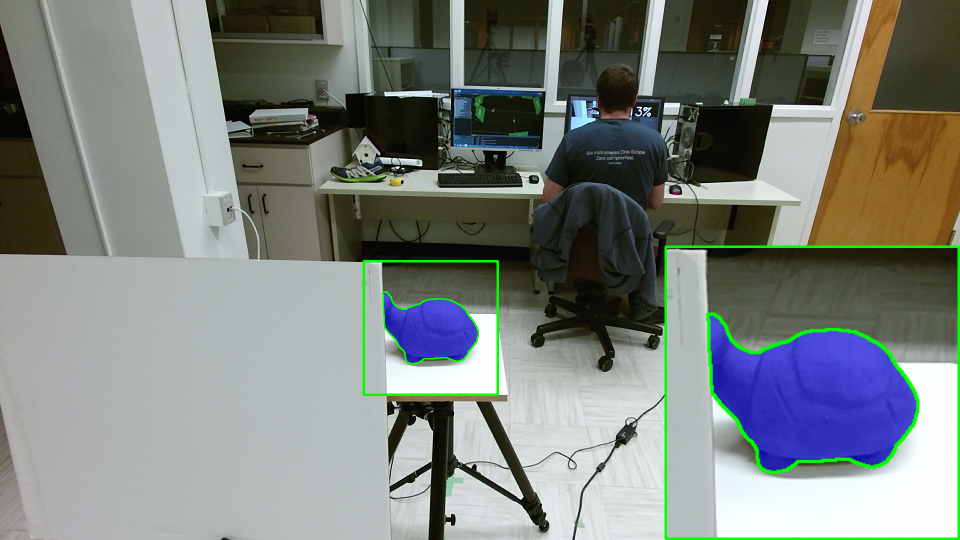
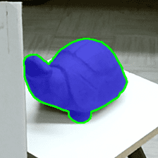
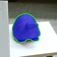
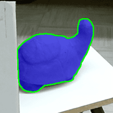
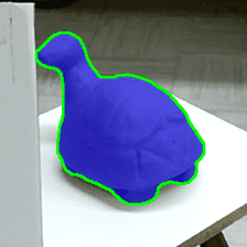
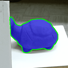
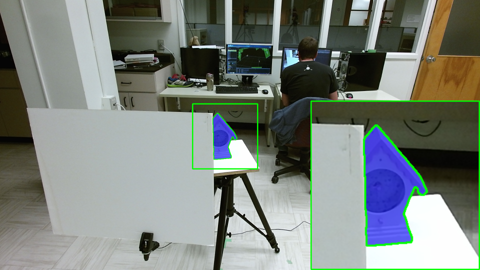
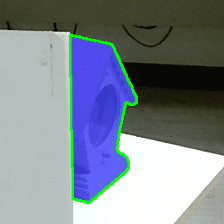
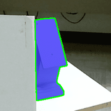
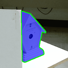
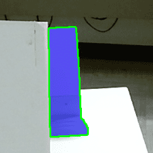
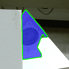
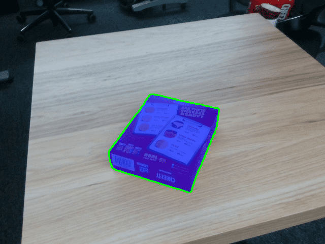
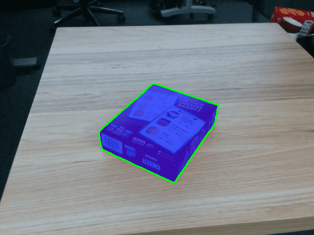
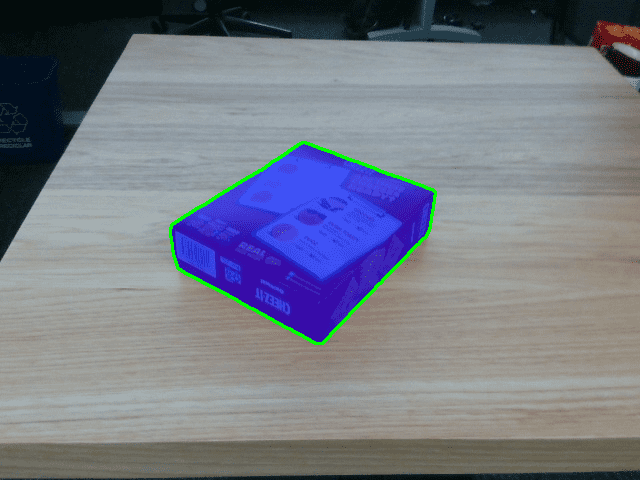
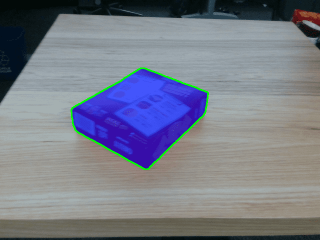
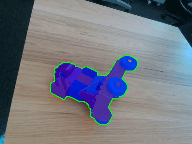
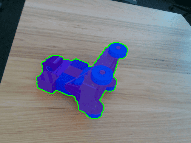
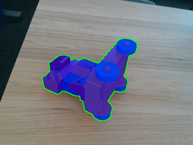
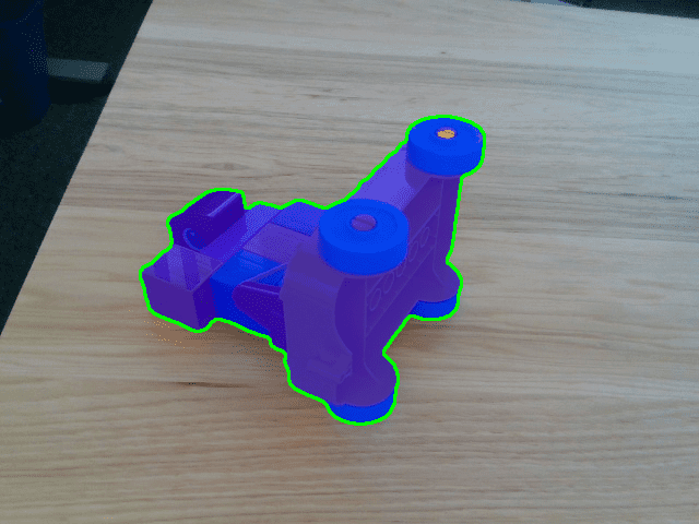
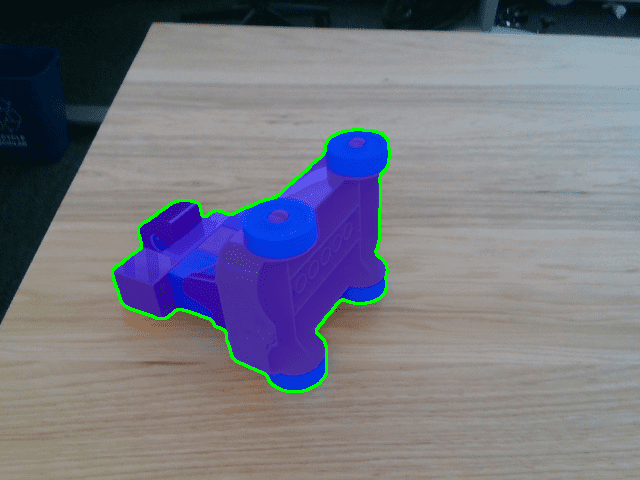
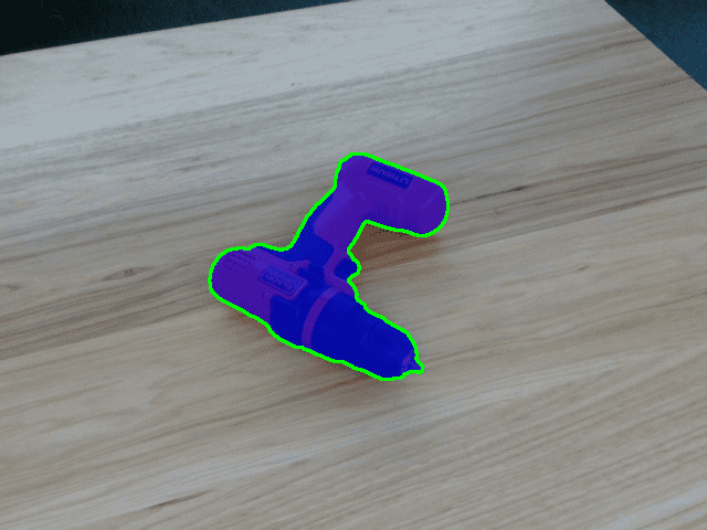
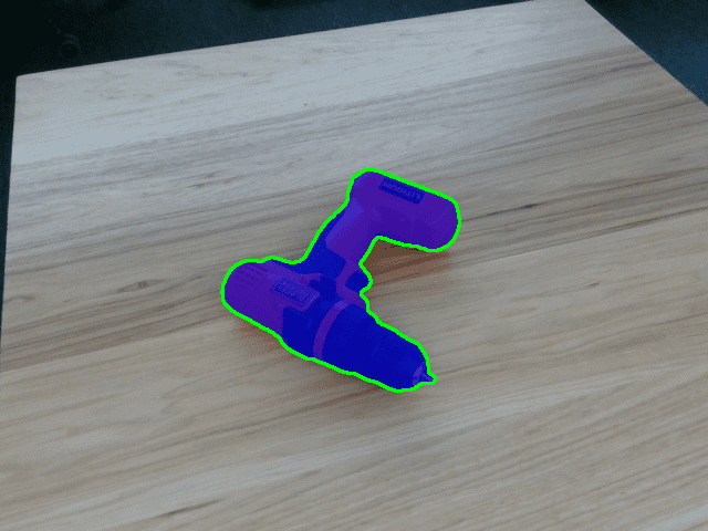
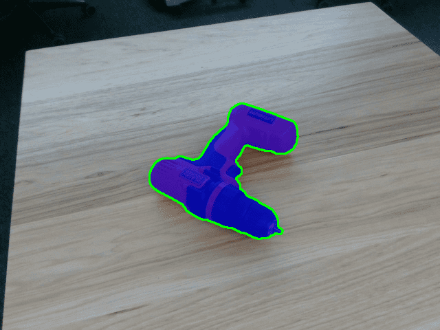
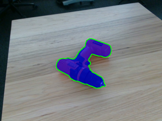
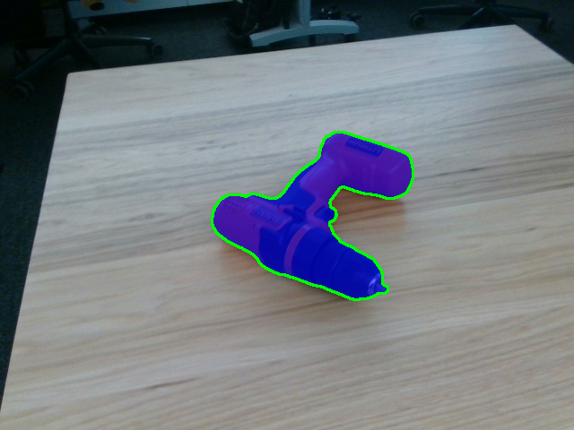
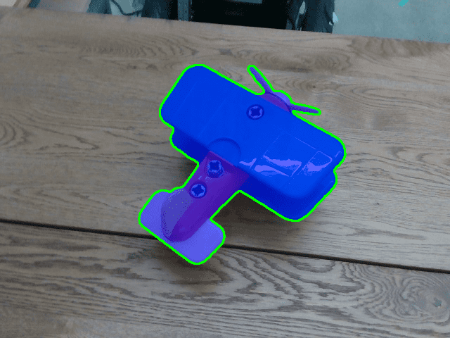
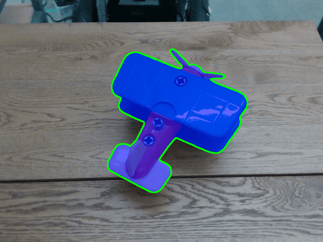
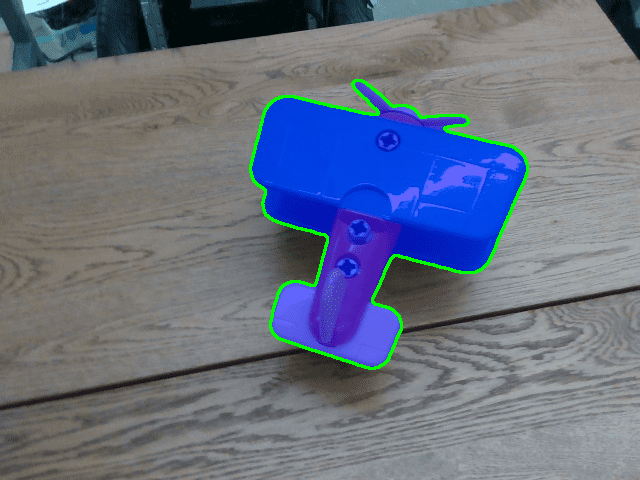
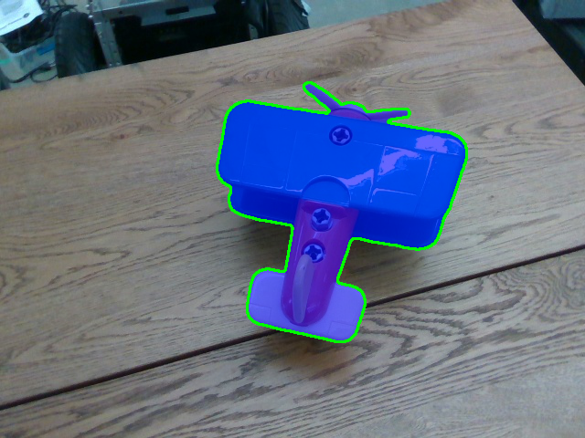
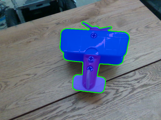
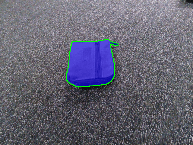
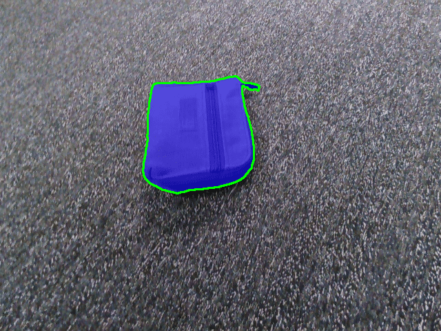
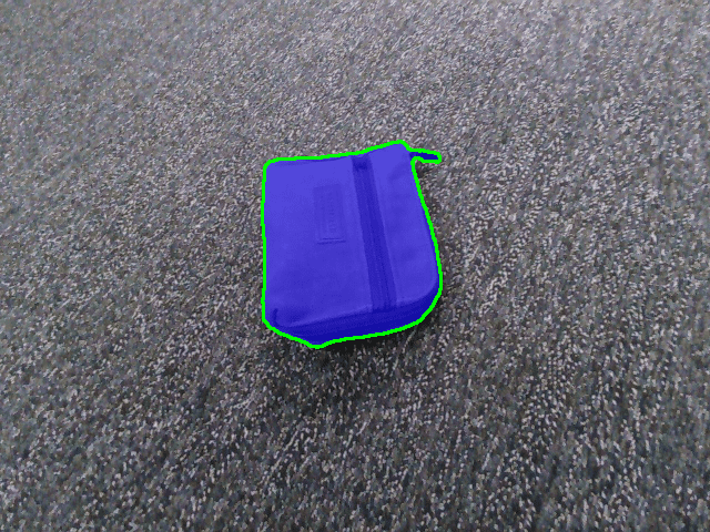
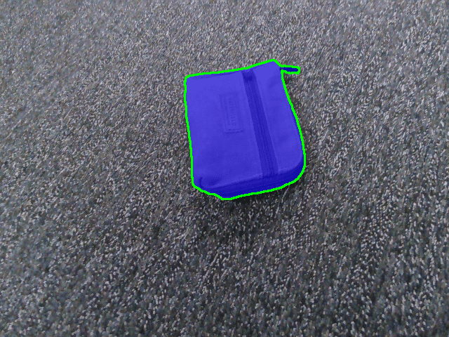
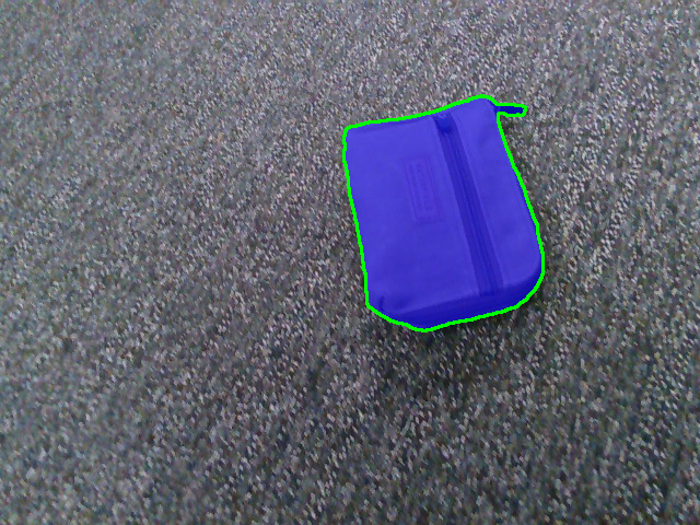
Figure 15: The segmentation model of [13] works surprisingly well on unseen objects. Results on Laval and Moped images.

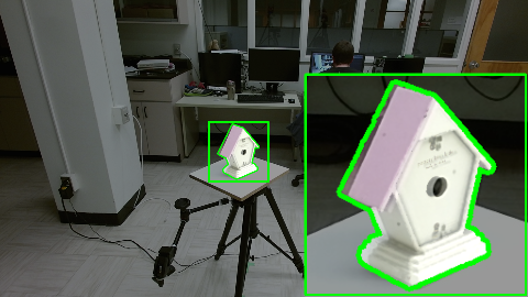
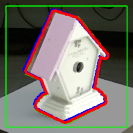
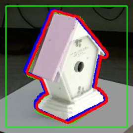
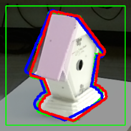
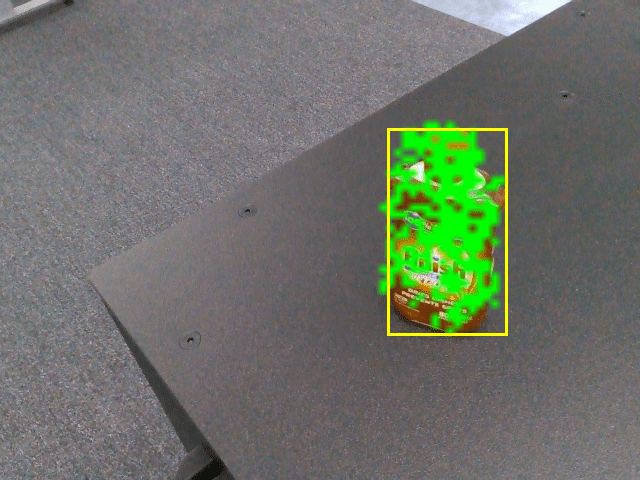
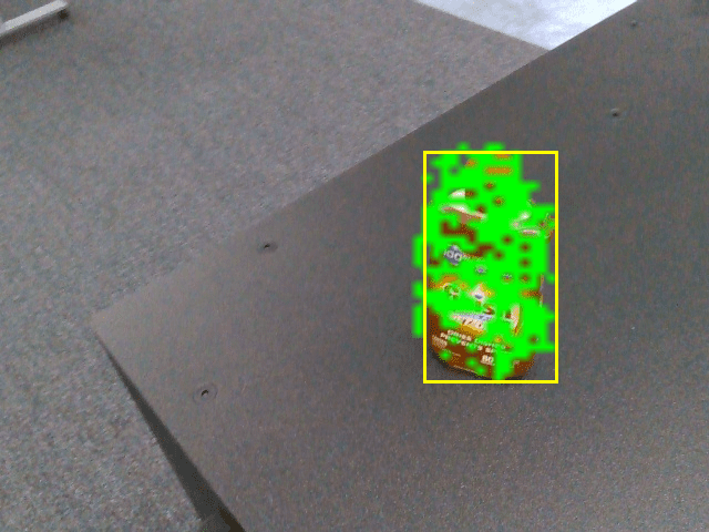
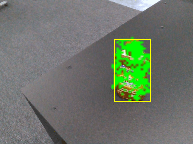
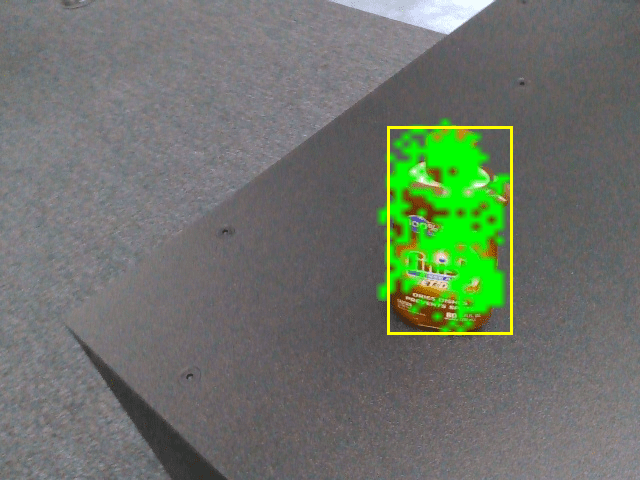
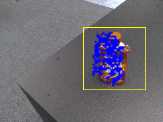
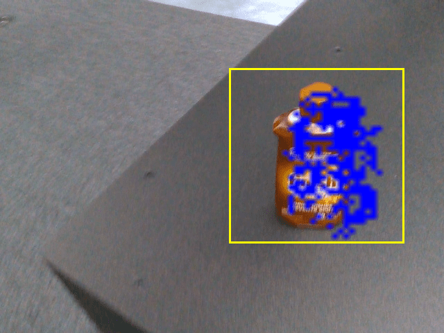
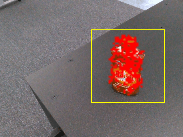
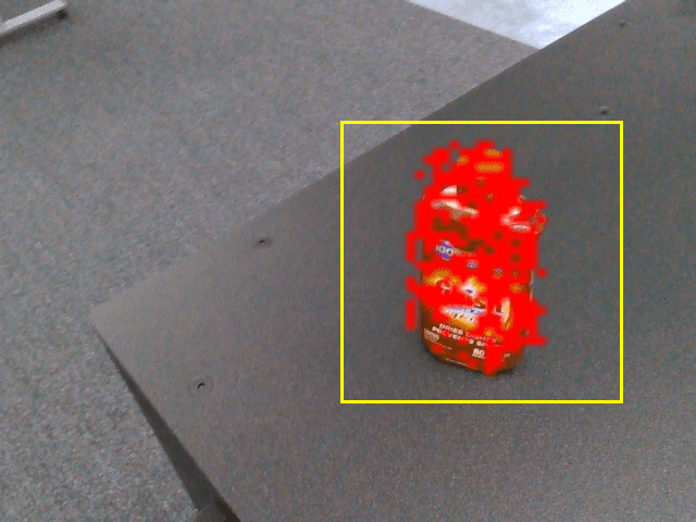
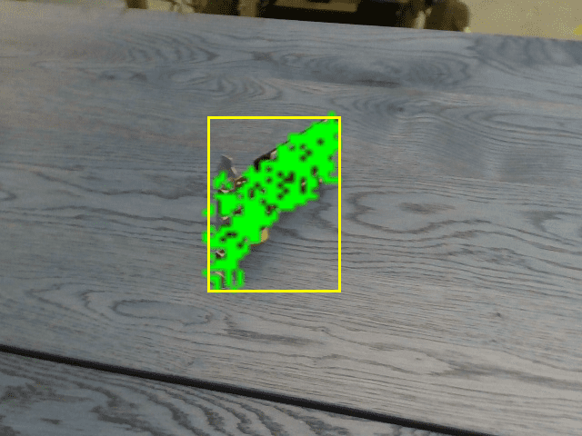
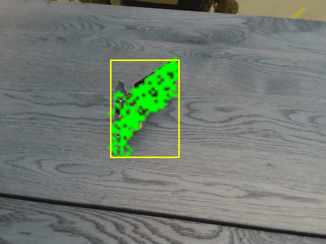
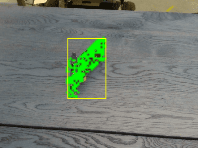
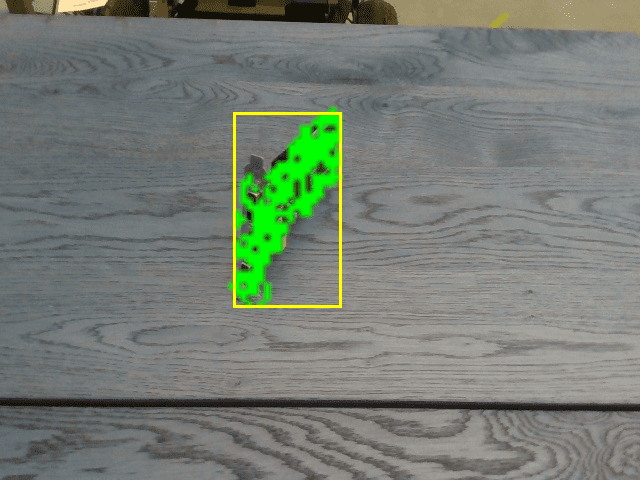
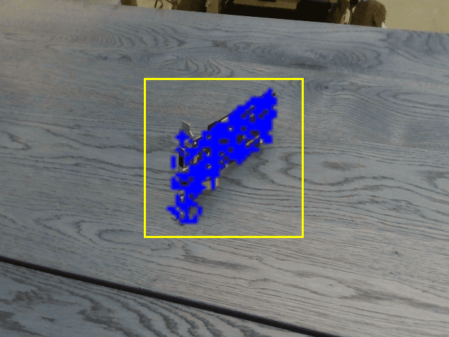
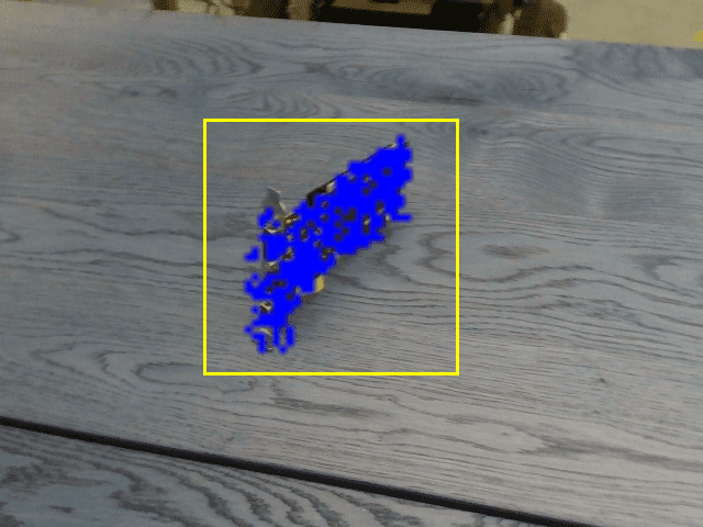
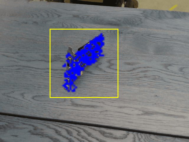
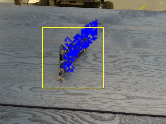
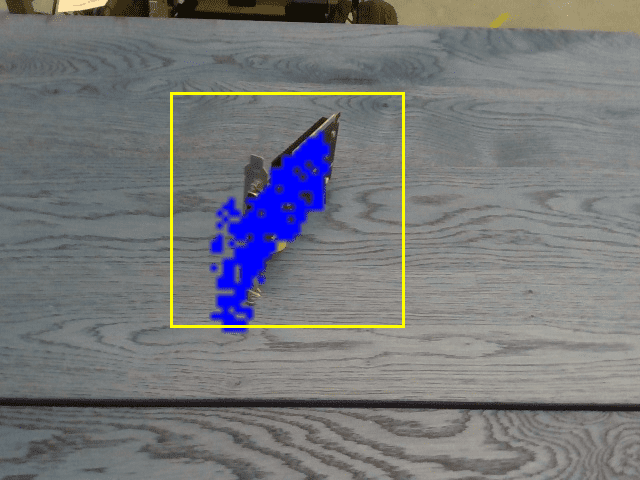
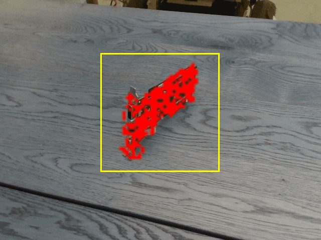
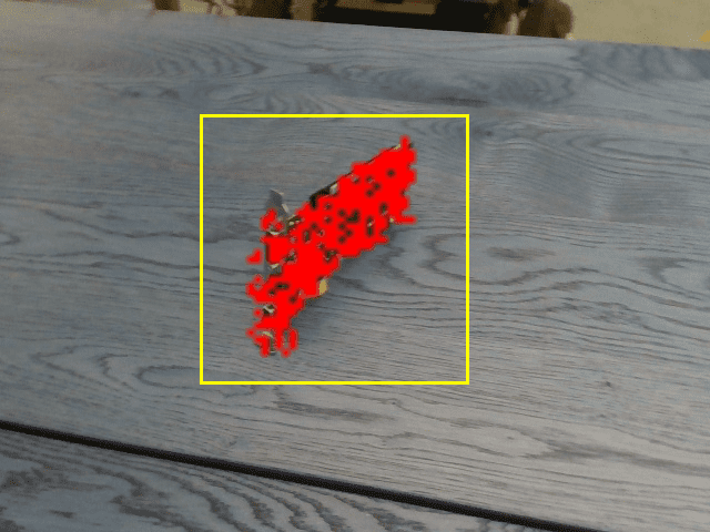
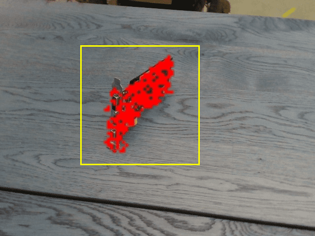
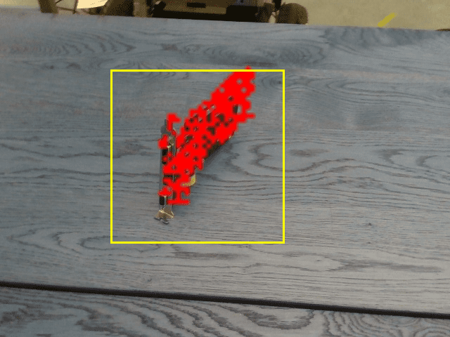
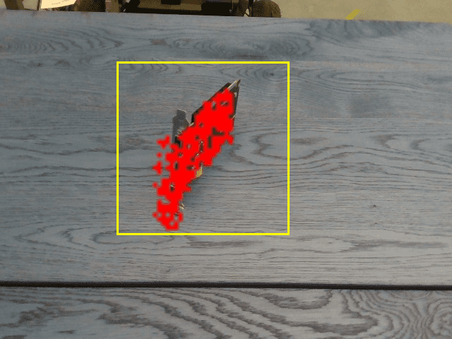
Figure 16: Qualitative results on real-world datasets. We show in each image the ground-truth in green, the prediction with Ours two-frame in blue and the prediction with Ours multi-frame in red. Two first rows show our results on two sequences of object “clock” and “kinect” of Laval dataset [16]. The six last rows show our results on two sequences of object “rinse_aid” and “graphic_card” of Moped dataset [33].

References

- [1] Denninger, Maximilian and Sundermeyer, Martin and Winkelbauer, Dominik and Zidan, Youssef and Olefir, Dmitry and Elbadrawy, Mohamad and Lodhi, Ahsan and Katam, Harinandan BlenderProc. In arXiv Preprint, 2019.
- [2] Zhou, Yi and Barnes, Connelly and Jingwan, Lu and Jimei, Yang and Hao, Li On the Continuity of Rotation Representations in Neural Networks. In IEEE Conference on Computer Vision and Pattern Recognition, 2019.
- [3] Kaskman, Roman and Zakharov, Sergey and Shugurov, Ivan and Ilic, Slobodan Homebreweddb: Rgb-D Dataset for 6D Pose Estimation of 3D Objects. In Proceedings of the IEEE/CVF International Conference on Computer Vision Workshops, 2019.
- [4] Rennie, Colin and Shome, Rahul and Bekris, Kostas E. and De Souza, Alberto F. A Dataset for Improved Rgbd-Based Object Detection and Pose Estimation for Warehouse Pick-And-Place. In IEEE Robotics and Automation Letters, 2016.
- [5] Aitor Aldoma, Federico Tombari, Johan Prankl, Andreas Richtsfeld, Luigi Di Stefano, and Markus Vincze. Multimodal Cue Integration through Hypotheses Verification for RGB-D Object Recognition and 6DOF Pose Estimation. In International Conference on Robotics and Automation, 2013.
- [6] Vassileios Balntas, Andreas Doumanoglou, Caner Sahin, Juil Sock, Rigas Kouskouridas, and Tae-Kyun Kim. Pose Guided RGBD Feature Learning for 3D Object Pose Estimation. In International Conference on Computer Vision, 2017.
- [7] Eric Brachmann, Alexander Krull, Frank Michel, Stefan Gumhold, Jamie Shotton, and Carsten Rother. Learning 6D Object Pose Estimation Using 3D Object Coordinates. In European Conference on Computer Vision, 2014.
- [8] Benjamin Busam, Hyun Jun Jung, and Nassir Navab. I Like to Move It: 6D Pose Estimation as an Action Decision Process. In arXiv Preprint, 2020.
- [9] Angel X. Chang, Thomas Funkhouser, Leonidas Guibas, Pat Hanrahan, Qixing Huang, Zimo Li, Silvio Savarese, Manolis Savva, Shuran Song, Hao Su, and Others. ShapeNet: An information-Rich 3D Model Repository. In arXiv Preprint, 2015.
- [10] Xu Chen, Zijian Dong, Jie Song, Andreas Geiger, and Otmar Hilliges. Category Level Object Pose Estimation via Neural Analysis-by-Synthesis. In European Conference on Computer Vision, 2020.
- [11] Changhyun Choi and Henrik I. Christensen. RGB-D Object Tracking: A Particle Filter Approach on GPU. In International Conference on Intelligent Robots and Systems, 2013.
- [12] Xinke Deng, Arsalan Mousavian, Yu Xiang, Fei Xia, Timothy Bretl, and Dieter Fox. PoseRBPF: A Rao-Blackwellized Particle Filter for 6D Object Pose Tracking. In Robotics: Science and Systems Conference, 2019.
- [13] Yuming Du, Wen Guo, Yang Xiao, and Vincent Lepetit. 1st Place Solution for the UVO Challenge on Video-Based Open-World Segmentation 2021. In arXiv Preprint, 2021.
- [14] Yuming Du, Yang Xiao, and Vincent Lepetit. Learning to Better Segment Objects from Unseen Classes with Unlabeled Videos. In International Conference on Computer Vision, 2021.
- [15] Mathieu Garon and Jean-François Lalonde. Deep 6-DOF Tracking. IEEE Transactions on Visualization and Computer Graphics, 23(11), 2017.
- [16] Mathieu Garon, Denis Laurendeau, and Jean-François Lalonde. A Framework for Evaluating 6DOF Object Trackers. In European Conference on Computer Vision, 2018.
- [17] Alexander Grabner, Peter Roth, and Vincent Lepetit. Location Field Descriptor: Single Image 3D Model Retrieval in the Wild. In International Conference on 3D Vision, 2019.
- [18] Kaiming He, Xiangyu Zhang, Shaoqing Ren, and Jian Sun. Deep Residual Learning for Image Recognition. In IEEE Conference on Computer Vision and Pattern Recognition, 2016.
- [19] Stefan Hinterstoißer, Vincent Lepetit, Slobodan Ilic, Stefan Holzer, Gary R. Bradski, Kurt Konolige, and Nassir Navab. Model Based Training, Detection and Pose Estimation of Texture-Less 3D Objects in Heavily Cluttered Scenes. In Asian Conference on Computer Vision, 2012.
- [20] Tomás Hodan, Pavel Haluza, Stepán Obdrzálek, Jiri Matas, Manolis I. A. Lourakis, and Xenophon Zabulis. T-LESS: An RGB-D Dataset for 6D Pose Estimation of Texture-Less Objects. In IEEE Winter Conference on Applications of Computer Vision, 2017.
- [21] Tomas Hodan, Frank Michel, Eric Brachmann, Wadim Kehl, Anders Glentbuch, Dirk Kraft, Bertram Drost, Joel Vidal, Stephan Ihrke, Xenophon Zabulis, and Others. Bop: Benchmark for 6D Object Pose Estimation. In European Conference on Computer Vision, 2018.
- [22] Yinlin Hu, Joachim Hugonot, Pascal Fua, and Mathieu Salzmann. Segmentation-Driven 6D Object Pose Estimation. In IEEE Conference on Computer Vision and Pattern Recognition, 2019.
- [23] Wadim Kehl, Fabian Manhardt, Federico Tombari, Slobodan Ilic, and Nassir Navab. SSD-6D: Making RGB-Based 3D Detection and 6D Pose Estimation Great Again. In International Conference on Computer Vision, 2017.
- [24] Alexander Krull, F. Michel, Eric Brachmann, S. Gumhold, Stephan Ihrke, and C. Rother. 6DOF Model Based Tracking via Object Coordinate Regression. In Asian Conference on Computer Vision, 2014.
- [25] Junghyun Kwon, Minseok Choi, Frank Park, and Changmook Chun. Particle Filtering on the Euclidean Group: Framework and Applications. Robotica, 25, 2007.
- [26] Yann Labbé, Justin Carpentier, Mathieu Aubry, and Josef Sivic. CosyPose: Consistent Multi-View Multi-Object 6D Pose Estimation. In European Conference on Computer Vision, 2020.
- [27] Yi Li, Gu Wang, Xiangyang Ji, Yu Xiang, and Dieter Fox. DeepIM: Deep Iterative Matching for 6D Pose Estimation. In European Conference on Computer Vision, 2018.
- [28] Zhigang Li, Gu Wang, and Xiangyang Ji. CDPN: Coordinates-Based Disentangled Pose Network for Real-Time RGB-Based 6DoF Object Pose Estimation. In International Conference on Computer Vision, 2019.
- [29] Yuan Liu, Yilin Wen, Sida Peng, Cheng Lin, Xiaoxiao Long, Taku Komura, and Wenping Wang. Gen6D: Generalizable Model-Free 6DoF Object Pose Estimation from RGB Images. In arXiv Preprint, 2022.
- [30] Ze Liu, Yutong Lin, Yue Cao, Han Hu, Yixuan Wei, Zheng Zhang, Stephen Lin, and Baining Guo. Swin Transformer: Hierarchical Vision Transformer Using Shifted Windows. In International Conference on Computer Vision, 2021.
- [31] Fabian Manhardt, Gu Wang, Benjamin Busam, M. Nickel, Sven Meier, Luca Minciullo, Xiangyang Ji, and N. Navab. CPS++: Improving Class-Level 6D Pose and Shape Estimation from Monocular Images with Self-Supervised Learning. In arXiv Preprint, 2020.
- [32] Van Nguyen Nguyen, Yinlin Hu, Yang Xiao, Mathieu Salzmann, and Vincent Lepetit. Templates for 3d object pose estimation revisited: Generalization to new objects and robustness to occlusions. In IEEE Conference on Computer Vision and Pattern Recognition, 2022.
- [33] Keunhong Park, Arsalan Mousavian, Yu Xiang, and Dieter Fox. LatentFusion: End-to-End Differentiable Reconstruction and Rendering for Unseen Object Pose Estimation. In IEEE Conference on Computer Vision and Pattern Recognition, 2020.
- [34] Kiru Park, Tim Patten, and Markus Vincze. Pix2Pose: Pixel-Wise Coordinate Regression of Objects for 6D Pose Estimation. In International Conference on Computer Vision, 2019.
- [35] Kiru Park, Timothy Patten, and Markus Vincze. Neural Object Learning for 6D Pose Estimation Using a Few Cluttered Images. In European Conference on Computer Vision, 2020.
- [36] Adam Paszke, Sam Gross, Soumith Chintala, Gregory Chanan, Edward Yang, Zachary DeVito, Zeming Lin, Alban Desmaison, Luca Antiga, and Adam Lerer. Automatic Differentiation in Pytorch. In NIPS Workshop, 2017.
- [37] Sida Peng, Yuan Liu, Qixing Huang, Xiaowei Zhou, and Hujun Bao. PVNet: Pixel-Wise Voting Network for 6DoF Pose Estimation. In IEEE Conference on Computer Vision and Pattern Recognition, 2019.
- [38] Giorgia Pitteri, Aurélie Bugeau, Slobodan Ilic, and Vincent Lepetit. 3D Object Detection and Pose Estimation of Unseen Objects in Color Images with Local Surface EMbeddings. In Asian Conference on Computer Vision, 2020.
- [39] Mahdi Rad and Vincent Lepetit. BB8: A Scalable, Accurate, Robust to Partial Occlusion Method for Predicting the 3D Poses of Challenging Objects Without Using Depth. In International Conference on Computer Vision, 2017.
- [40] Ivan Shugurov, Fu Li, Benjamin Busam, and Slobodan Ilic. Osop: A multi-stage one shot object pose estimation framework. In IEEE Conference on Computer Vision and Pattern Recognition, 2022.
- [41] Jiaming Sun, Zihao Wang, Siyu Zhang, Xingyi He, Hongcheng Zhao, Guofeng Zhang, and Xiaowei Zhou. OnePose: One-Shot Object Pose Estimation Without CAD Models. In arXiv Preprint, 2022.
- [42] Martin Sundermeyer, Maximilian Durner, En Yen Puang, Zoltán-Csaba Márton, and Rudolph Triebel. Multi-Path Learning for Object Pose Estimation Across Domains. In IEEE Conference on Computer Vision and Pattern Recognition, 2020.
- [43] Martin Sundermeyer, Zoltan-Csaba Marton, Maximilian Durner, Manuel Brucker, and Rudolph Triebel. Implicit 3D Orientation Learning for 6D Object Detection from RGB Images. In European Conference on Computer Vision, 2018.
- [44] David J. Tan and Slobodan Ilic. Multi-Forest Tracker: A Chameleon in Tracking. In IEEE Conference on Computer Vision and Pattern Recognition, 2014.
- [45] David J. Tan, Federico Tombari, Slobodan Ilic, and Nassir Navab. A Versatile Learning-Based 3D Temporal Tracker: Scalable, Robust, Online. In International Conference on Computer Vision, 2015.
- [46] Jim Taylor, Jamie Shotton, Tony Sharp, and Aandrew Fitzgibbon. The Vitruvian Manifold: Inferring Dense Correspondences for One-Shot Human Pose Estimation. In IEEE Conference on Computer Vision and Pattern Recognition, 2012.
- [47] Zachary Teed and Jia Deng. Raft: Recurrent All-Pairs Field Transforms for Optical Flow. In European Conference on Computer Vision, 2020.
- [48] Bugra Tekin, Sudipta N. Sinha, and Pascal Fua. Real-Time Seamless Single Shot 6D Object Pose Prediction. In IEEE Conference on Computer Vision and Pattern Recognition, 2018.
- [49] Hung-Yu Tseng, Shalini De Mello, Jonathan Tremblay, Sifei Liu, Stan Birchfield, Ming-Hsuan Yang, and Jan Kautz. Few-Shot Viewpoint Estimation. In British Machine Vision Conference, 2019.
- [50] Chen Wang, Roberto Martín-Martín, Danfei Xu, Jun Lv, Cewu Lu, Li Fei-Fei, Silvio Savarese, and Yuke Zhu. 6-PACK: Category-Level 6D Pose Tracker with Anchor-Based Keypoints. In International Conference on Robotics and Automation, 2020.
- [51] He Wang, Srinath Sridhar, Jingwei Huang, Julien Valentin, Shuran Song, and Leonidas J. Guibas. Normalized Object Coordinate Space for Category-Level 6D Object Pose and Size Estimation. In IEEE Conference on Computer Vision and Pattern Recognition, 2019.
- [52] Weiyao Wang, Matt Feiszli, Heng Wang, and Du Tran. Unidentified Video Objects: A Benchmark for Dense, Open-World Segmentation. In International Conference on Computer Vision, 2021.
- [53] Bowen Wen and Kostas Bekris. Bundletrack: 6D Pose Tracking for Novel Objects Without Instance or Category-Level 3D Models. In International Conference on Intelligent Robots and Systems, 2021.
- [54] Paul Wohlhart and Vincent Lepetit. Learning Descriptors for Object Recognition and 3D Pose Estimation. In IEEE Conference on Computer Vision and Pattern Recognition, 2015.
- [55] Zhirong Wu, Shuran Song, Aditya Khosla, Fisher Yu, Linguang Zhang, Xiaoou Tang, and Jianxiong Xiao. 3D Shapenets: A Deep Representation for Volumetric Shapes. In IEEE Conference on Computer Vision and Pattern Recognition, 2015.
- [56] Yu Xiang, Tanner Schmidt, Venkatraman Narayanan, and Dieter Fox. PoseCNN: A Convolutional Neural Network for 6D Object Pose Estimation in Cluttered Scenes. In Robotics: Science and Systems Conference, 2018.
- [57] Tete Xiao, Yingcheng Liu, Bolei Zhou, Yuning Jiang, and Jian Sun. Unified Perceptual Parsing for Scene Understanding. In European Conference on Computer Vision, 2018.
- [58] Sergey Zakharov, Ivan S. Shugurov, and Slobodan Ilic. DPOD: 6D Pose Object Detector and Refiner. In International Conference on Computer Vision, 2019.
- [59] Huizhong Zhou, Benjamin Ummenhofer, and Thomas Brox. DeepTAM: Deep Tracking and Mapping. In European Conference on Computer Vision, 2018.