Combinatorial geometry of neural codes, neural data analysis, and neural networks

Mathematics August 2022 for a baccalaureate degree
in Engineering Science
with honors in Engineering Science Dissertation The Graduate School 4 Honors P. Advisor Associate Professor of Engineering Science and Mechanics Honors P. Advisor, Jr. Professor of Engineering Science and Mechanics Second T. Supervisor Mark Levi Professor of Mathematics [Dissertation Advisor][Chair of Committee] Carina Curto Professor of Mathematics Vladimir Itskov Associate Professor of Mathematics Jason Morton Associate Professor of Mathematics Réka Albert Distinguished Professor of Physics and Biology Alexei Novikov Professor of Mathematics, Associate Head for Graduate Studies

SupplementaryMaterial/Abstract

SupplementaryMaterial/Acknowledgments

Preliminaries

Introduction

Neural activity both encodes information about the outside world and arises from the activity of interacting neurons. Here, we will explore how both of these things happen. Which features of the world can be recovered from neural activity alone? What is the relationship between the structure of neural connectivity and the dynamics of neural activity? Answering these questions presents mathematical challenges, which we consider here. Quantitative data is often hidden not just by noise, but by nonlinear distortion or missing information that makes traditional data analysis and modeling techniques less useful. When quantitative details are lost, combinatorial information remains. With tools from discrete geometry, we can use this combinatorial information to constrain the underlying geometry. Using nonlinear dynamics, we show how the graph structure of a neural circuit constrains its dynamics.

The first problem we consider, in Chapters Introduction to Convex Neural Codes, Order Forcing in Neural Codes, and Oriented Matroids and Convex Neural Codes, concerns convex neural codes. One common way neurons encode information about the world is via receptive field coding: each neuron has a set of stimuli, known as its receptive field, and fires when the animal receives a stimulus within this receptive field. In 2014, John O’Keefe won the Nobel prize for the 1976 discovery of place cells, neurons whose receptive fields, termed place fields, are regions of the environment [1]. When an animal is located within the place field of a given neuron, that place cell fires at an increased rate. Though receptive field coding occurs in many other contexts, we will focus on place cells as our primary example of receptive field coding.

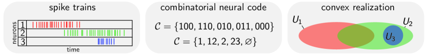
Figure 1: Convex neural codes arise from the activity of neurons with convex receptive fields. Spike trains (left) can be proccessed into a combinatorial neural code (center), which records which sets of neurons fire at the same time. This code is convex if it is the intersection pattern of a family of convex open sets (right). Convex sets correspond to receptive fields, regions of the stimulus space to which the neurons respond.

Notice that it is in principle possible to recover from neural activity alone which place fields overlap: a set of place fields has a nonempty intersection if the corresponding place cells are active at the same time. We formalize this using a simplified model of place cells in which each neuron’s receptive field is a subset of Euclidean space $U_{i}\subseteq\mathbb{R}^{d}$. Each neuron is active if and only if the animal is located which this neuron’s place field. We refer to the set of active neurons corresponding to each point in space as a codeword $\sigma\subseteq[n]:=\{1,\ldots,n\}$. We can describe the set of codewords arising from a family of place fields $U_{1},\ldots,U_{n}$ by

$$\operatorname{code}(U_{1},\ldots,U_{n}):=\{\sigma\mid\bigcap_{i\in\sigma}U_{i}\setminus\bigcup_{j\notin\sigma}U_{j}\neq\varnothing\},$$

as illustrated in Figure 1.

Within small environments, place fields are roughly convex sets. A growing body of work [2, 3, 4, 5, 6, 7, 8, 9, 10, 11, 12, 13, 14, 15, 16, 17, 18, 19] explores what consequences this constraint on receptive field geometry has for combinatorial neural codes: which combinatorial neural codes arise from neurons with convex receptive fields? Given a combinatorial neural code $\mathcal{C}\subseteq 2^{[n]}$, when do there exist convex open sets $U_{1},\ldots,U_{n}$ such that $\mathcal{C}=\operatorname{code}(U_{1},\ldots,U_{n})$? This question turns out to be mathematically rich: it has connections to classic problems in discrete geometry which ask when a simplicial complex is representable as the nerve of a family of convex sets in $\mathbb{R}^{d}$ [20, 21, 22, 23] or when an oriented matroid is representable as a hyperplane arrangement [24, 25, 26]. In Chapter Order Forcing in Neural Codes, we introduce order-forcing as a technique for proving that codes are not convex. Our main result in this section is Theorem 0.7, which gives conditions for when a list of codewords must correspond to a straight line in every convex realization of a code. We use this result to construct several new examples of non-convex codes. Material in this paper is taken from [27]. In Chapter Oriented Matroids and Convex Neural Codes, we make the connection between convex codes and oriented matroids explicit. Our main results in this section are Theorem 0.1, which relates convex codes to oriented matroids via the code morphisms of [10], and Theorem 0.4, which states that recognizing convex codes is computationally intractable. Material in this chapter is taken from [11].

Next in Chapters A Novel Notion of Rank for Neural Data Analysis and The Geometry of Underlying Rank, we investigate a different aspect of the neural code, its dimensionality. The dimensionality of neural activity varies across experimental conditions, but is often observed to be low relative to the number of neurons recorded [28]. Low-dimensional activity can reflect the low-dimensional input or low-dimensional intrinsic dynamics [29, 30, 31, 32]. The optimal dimensionality of neural activity is subject to computational trade-offs: higher-dimensional neural representations allow more complex readouts by downstream networks, while lower-dimensional representations have better generalization properties [33, 34].

However, common measurement techniques such as calcium imaging can distort firing rates in a nonlinear way, which can cause problems for typical methods of estimating dimensionality [35, 36]. However, we do expect this distortion to roughly monotone, and thus to preserve the ordering between measurements. Can we use this information to estimate dimensionality?

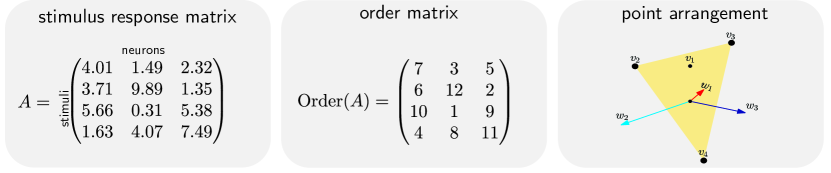
Figure 2: The underlying rank of a matrix is the lowest rank consistent with the ordering of entries. The only reliable information contained in neural data (left) after an unknown monotone transformation is the ordering of entries (center). We introduce techniques for estimating underlying rank by using the order matrix to infer information about an underlying point arrangement (right).

Motivated by this problem, we introduce the underlying rank of a matrix $A$ as the minimal value of $d$ such that there is a rank $d$ matrix whose entries are in the same order as those of $A$. The general idea of using the order of entries in a matrix to determine information about geometric structure is introduced in [37], and is approached topologically in that paper and in [38]. See Figure 2 for an overview of the underlying rank? We show that matrices with underlying rank $d$ correspond to point arrangements in $\mathbb{R}^{d}$, and that it is possible to recover information about this point arrangement using the ordering of entries in $A$. Much like the convex neural codes problem, underlying rank has natural connections to the theory of allowable sequences [39] and oriented matroids [40]. In Chapter A Novel Notion of Rank for Neural Data Analysis, we introduce the underlying rank and some tools for estimating it. Our main contributions in this chapter are as follows: We define minimal nodes, and prove Propositions 0.10, 0.11, and 0.12, which relate the expected number of minimal nodes to the rank of a random matrix. We also define the Radon rank of a matrix and prove that it is a lower bound for underlying rank in Proposition 0.16. In Chapter The Geometry of Underlying Rank, we explore underlying rank in greater mathematical detail. The main results of this chapter are Examples 0.8 and 0.10, matrices whose underlying rank exceeds their Radon rank. Example 0.8 arises from the relationship between underlying rank and oriented matroid theory which we describe in Theorem 0.2. Example 0.10 arises from the relationship between underlying rank and allowable sequences, which we describe in Observation 0.2. We also exploit this relationship between allowable sequences and underlying rank to prove that computing underlying rank is computationally intractable in Corollary 0.3.

Finally, in Chapters LABEL:chapter:TLNs1, LABEL:chapter:nullclines, and LABEL:chapter:TLNs2, we turn to the relationship between the connectivity of a neural circuit and its dynamics. See Figure 3 for an overview of this relationship. Different computational tasks require different patterns of network activity: for instance, central pattern generators are networks which generate the periodic activity needed for walking, breathing, and other rhythmic activities. Viewed as dynamical systems, these networks need to have limit cycles. On the other hand, networks whose activity always converges to a stable fixed point, such as the Hopfield model, are used to model pattern completion in memory. How do different patterns of network connectivity contribute to these different types of activity?

In general, this question is difficult because neural circuits have nonlinear dynamics. We thus consider a simple, nonlinear model, threshold-linear networks (TLNs). In a TLN, the firing rate $x_{i}$ of neuron $i$ is determined by

$$\frac{dx_{i}}{dt} =-x_{i}+\left[\sum_{j=1}^{n}W_{ij}x_{j}+b_{i}\right]_{+},$$ (1)

where $\left[y\right]_{+}=\max\{y,0\}$. To isolate the role of connectivity, we consider a further restriction to combinatorial threshold-linear networks (CTLNs), whose dynamics are fully determined by a directed graph. A fair amount is known about how the stable and unstable fixed points of combinatorial threshold-linear networks are constrained by the graph, but less is known about their dynamic attractors more generally. In particular if a TLN is symmetric, then all trajectories approach stable fixed points by [41]. At the opposite extreme, if a graph has no bidirectional edges and no sinks, its CTLN has no stable fixed points, and thus must have a dynamic attractor.

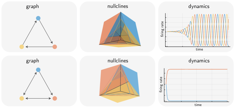
Figure 3: CTLNs are dynamical systems determined by directed graph. The directed graph of a CTLN (left) constrains the nullcline arrangement, which in turn constrains the dynamics.

Here, we begin to classify which CTLNs have dynamic attractors, which do not. In particular, we prove that the CTLN of a directed acyclic graph must have all trajectories converge to a fixed point. This result can be combined with the result about symmetric threshold-linear networks to prove that if a graph can be decomposed into a directed acyclic graph with edges onto a symmetric graph, all trajectories of its CTLN converge to a fixed point. Our results are sufficient to classify which three neuron graphs have dynamic attractors. Chapter LABEL:chapter:TLNs1 gives an introduction to CTLNs. Chapter LABEL:chapter:nullclines explores the nullcline arrangements of TLNs. The main result in this chapter is Theorem LABEL:thm:mixed_sign, which states that all trajectories of a competitive TLN approach in a small region defined by the nullclines. This results in Corollary LABEL:cor:total_pop, which bounds the total population activity of a TLN in terms of the weights. The bulk of our main results about CTLNs appear in Chapter LABEL:chapter:TLNs2. In particular, this chapter contains Theorems LABEL:thm:dag and LABEL:thm:dag_onto_symmetric, which give conditions which guarantee that all trajectories of a CTLN converge to a fixed point. Theorem LABEL:thm:dag covers the case of directed acyclic graphs, while Theorem LABEL:thm:dag_onto_symmetric strengthens this result to include graphs which contain a directed acyclic part and a symmetric part arranged in a particular way.

The structure of this dissertation is as follows: in Chapter Combinatorial Background, we give the common background on convex sets, hyperplane arrangements, point arrangements, and oriented matroids required for the subsequent chapters. In Part II, Chapters Introduction to Convex Neural Codes, Order Forcing in Neural Codes, and Oriented Matroids and Convex Neural Codes, we discuss convex neural codes. In Part III, Chapters A Novel Notion of Rank for Neural Data Analysis and The Geometry of Underlying Rank we discuss underlying rank. In Part IV, Chapters LABEL:chapter:TLNs1, LABEL:chapter:nullclines, and LABEL:chapter:TLNs2, we discuss threshold-linear networks.

My novel contributions are concentrated in Chapters 4, 5, 6, 7, 9, and 10. The results in Chapters 4 and 5 can be found in the papers Order Forcing in Neural Codes, written with Amzi Jeffs and Nora Youngs [27] and Oriented Matroids and Neural Codes, written with Alexander Kunin and Zvi Rosen [11]. The results on underlying rank in Chapters 6 and 7 and the results on TLNs in Chapters 9 and 10 are currently being written up for publication.

Combinatorial Background

In this chapter, we give background information on the combinatorial objects and theorems which are used here. In particular, we discuss convex neural codes, hyperplane arrangements, and oriented matroids. We use the notation $[n]:=\{1,\ldots,n\}$, and use $2^{[n]}:=\mathcal{P}([n])$ to denote the powerset of $[n]$.

Intersection patterns of convex sets

The nerve of a cover records the intersection pattern of a family of sets.

Definition 0.1.

Let $\mathcal{U}=\{U_{1},\ldots,U_{n}\}$ be a family of subsets of a set $X$. The nerve of $\mathcal{U}$, denoted $\operatorname{nerve}(\mathcal{U})$, is the simplicial complex

$$\operatorname{nerve}(\mathcal{U}):=\{\sigma\subseteq[n]\mid\bigcap_{i\in\sigma}U_{i}\neq\varnothing\}.$$

We use the notation $U_{\sigma}:=\bigcap_{i\in\sigma}U_{i}$, with $U_{\varnothing}=X$.

Notice that $\operatorname{nerve}(\mathcal{U})$ records less detail about a family of sets than $\operatorname{code}(\mathcal{U})$, defined in the previous section. Various versions of the nerve theorem, which relate the topology of the nerve to that of the underlying space, were proved in [42, 43, 44]. The version of the nerve theorem we use is [45, Corollary 4G.3], and holds when the members of $\mathcal{U}$ form a good cover.

Definition 0.2.

A family of sets $\mathcal{U}=\{U_{1},\ldots,U_{n}\}$ is a good cover if for all $\sigma\subseteq[n]$, $U_{\sigma}$ is either empty or contractible.

Notice that, since intersections of convex sets are convex, and convex sets are contractible, any collection of convex sets forms a good cover.

Theorem 0.1 (The Nerve Lemma [45]).

Let $\mathcal{U}=\{U_{1},\ldots,U_{n}\}$ be a good cover, with all sets open or all sets closed. Then $\operatorname{nerve}(U)$ is homotopy equivalent to $\bigcup_{i=1}^{n}U_{i}$.

Every simplicial complex arises as the nerve of a family of convex sets [23]. However, characterizing the dimension required is more complicated. A simplicial complex $\Delta$ is $d$-representable if $\Delta=\operatorname{nerve}(\mathcal{U})$ where $\mathcal{U}$ is a family of convex open sets in $\mathbb{R}^{d}$.

A classic theorem in the vein is Helly’s theorem, which constrains the intersection pattern of convex sets in $\mathbb{R}^{d}$.

Theorem 0.2 (Helly’s theorem [46]).

Let $\mathcal{U}=\{U_{1},\ldots,U_{n}\}$ be a family of convex sets in $\mathbb{R}^{d}$. Define $U_{\sigma}=\bigcap_{i\in\sigma}U_{i}$. Then if for each $\sigma\subseteq[n]$ with $|\sigma|=d+1$ has $U_{\sigma}\neq\varnothing$, then $U_{[n]}\neq\varnothing$.

Interpreted as a result about $d$-representability, Helly’s theorem states that if a $d$-representable simplicial complex contains every $d$-simplex, then it is a simplex. Helly’s theorem holds when the family of convex sets is replaced with a good cover, and is a consequence of the nerve theorem. More general results in this vein exist, characterizing $f$-vectors of $d$-representable complexes [20, 21, 47]. Other results characterize $d$-representable complexes topologically and combinatorially: $d$-representable complexes must be $d$-collapsible [48].

In particular, the problem of determining the minimal dimension $d$ such that $\Delta$ arises as the nerve of convex sets in $\mathbb{R}^{d}$ is is NP-hard [49]. Further, the minimal dimension $d$ for which $\Delta$ arises as the nerve of a good cover may be lower than that in which $\Delta$ arises as the nerve of a family of convex sets [50].

Note that if a combinatorial code $\mathcal{C}$ is a simplicial complex, then convexity in a certain dimension corresponds to $d$-representability. Thus, the theory of convex codes which we will discuss in Chapters Introduction to Convex Neural Codes, Order Forcing in Neural Codes, and Oriented Matroids and Convex Neural Codes strictly generalizes the theory of $d$-representability.

Hyperplane and point arrangements

Hyperplane arrangements and point arrangements are both ways of giving a geometric structure to the relationships between the columns of a matrix. We will make extensive use of hyperplane arrangements, via oriented matroid theory, in Chapter Oriented Matroids and Convex Neural Codes, and will use them to a lesser extent in Chapters LABEL:chapter:TLNs1, LABEL:chapter:nullclines, and LABEL:chapter:TLNs2. We will use point arrangements heavily in Chapters A Novel Notion of Rank for Neural Data Analysis and The Geometry of Underlying Rank.

Arrangements of hyperplanes, and the half-spaces they define, form an important special case of arrangements of convex sets. A vector $h\in\mathbb{R}^{d}$ defines a hyperplane $H$ and two open half-spaces $H^{+}$ and $H^{-}$ by

$$H:=\{x\mid h\cdot x=0\} H^{+}:=\{x\mid h\cdot x>0\} H^{-}:=\{x\mid h\cdot x<0\}.$$

$H^{+}$ and $H^{-}$ are referred to as the positive and negative sides of $H$, respectively. A set of hyperplanes is called a hyperplane arrangement. A hyperplane arrangement is essential if the matrix with columns $h_{1},\ldots,h_{n}$ has rank $d$. Notice that under this definition, all hyperplanes meet at the origin. We can also define affine hyperplane arrangements. An affine hyperplane is defined by

$$H:=\{x\mid h\cdot x+b=0\} H^{+}:=\{x\mid h\cdot x+b>0\} H^{-}:=\{x\mid h\cdot x+b<0\}.$$

An arrangement which is not affine as central. We can translate between central and affine hyperplane arrangements, embedding any affine arrangement in $\mathbb{R}^{d}$ as a central arrangement in $\mathbb{R}^{d+1}$. More specifically, let $h=(h_{1},\ldots,h_{d}),b$ define an affine hyperplane. Then $\hat{h}=(h_{1},\ldots,h_{d},b)$ defines a central hyperplane in $\mathbb{R}^{d+1}$. Restricting to the plane $x_{d+1}=1$ recovers our original affine hyperplane arrangement.

An arrangement of $n$ hyperplanes in $\mathbb{R}^{d}$ divides space into a union of at most $2^{n}$ full dimensional chambers. Each of these chambers corresponds to a facet of $\operatorname{nerve}(H_{1}^{+},H_{1}^{-},\ldots,H_{n}^{+},H_{n}^{-})$, a simplicial complex on the vertex set $\{1,\ldots,n\}\cup\{\bar{1},\ldots,\bar{n}\}$ known as the polar complex in [12]. A set $\sigma\cup\tau$, $\sigma\subseteq\{1,\ldots,n\},\tau\subseteq\{\bar{1},\ldots,\bar{n}\}$ is a face of $\operatorname{nerve}(H_{1}^{+},H_{1}^{-},\ldots,H_{n}^{+},H_{n}^{-})$ if and only if there is some point $p\in\mathbb{R}^{d}$ such that $h_{i}\cdot p>0$ for $i\in\sigma$, $h_{j}\cdot p<0$ for $\bar{j}\in\tau$. While every simplicial complex arises as the nerve of some arrangement of convex sets, this is not true when we replace “convex sets" with half spaces. In general, it is difficult to determine whether a simplicial complex is the nerve of an arrangement of half-spaces. On the other hand, it is possible to recover the dimension of an essential hyperplane arrangement from its nerve.

To see this, we notice that the half spaces $H_{1}^{+},H_{1}^{-},\ldots,H_{n}^{+},H_{n}^{-}$ cover all of $\mathbb{R}^{d}$, except for the point $\bigcap_{i=1}^{n}H_{i}$. Thus, the nerve of a central, essential arrangement in $\mathbb{R}^{d}$ has the homotopy type of a $d-1$ sphere, while the nerve of an affine arrangement is contractible. Notice that when the maximal value of $2^{n}$ chambers is achieved, $\operatorname{nerve}(H_{1}^{+},H_{1}^{-},\ldots,H_{n}^{+},H_{n}^{-})$ is a $n$-dimensional cross polytope. This means that the maximal value can be achieved only when $d=n$ and $H_{1},\ldots,H_{n}$ is an essential arrangement.

If $H_{1},\ldots,H_{n}$ are an essential hyperplane arrangement in $\mathbb{R}^{d}$, then there is some $\sigma\subseteq[n]$ such that the normal vectors to $\{H_{i}\}_{i\in\sigma}$ span $\mathbb{R}^{d}$. Then restricting the nerve to this subset produces a $d$-dimensional cross polytope, with $2^{d}$ facets. If we restrict to any larger set of hyperplanes, there must be some “missing facet". The complex $\operatorname{nerve}(H_{1}^{+},H_{1}^{-},\ldots,H_{n}^{+},H_{n}^{-})$ is studied in more detail in [12], in the context of convex neural codes.

The same numerical data used to define a hyperplane arrangement may also be taken to define a point arrangement $p_{1},\ldots,p_{n}\in\mathbb{R}^{d}$. We can describe the combinatorial structure of a point arrangement in terms of which sets of points can be separated with hyperplanes. In particular, there is an affine hyperplane separating the points $\{p_{i}\}_{i\in\sigma}$, $\{p_{j}\}_{i\in\tau}$ if and only if there is some vector $h\in\mathbb{R}^{d+1}$ such that $h\cdot(p_{i},1)>0$ for $i\in\tau$, $h\cdot(p_{j},1)<0$ for $j\in\sigma$. Notice that this is the same condition for $(\sigma,\tau)$ to be the chamber of a hyperplane arrangement. Thus, we can also determine dimension of a point arrangement from the partitions of points which can be achieved with a hyperplane–for any set of at $n$ points in $\mathbb{R}^{d}$, if $n\geq d+2$, there is some partition of the points which cannot be achieved with a hyperplane.

This observation is equivalent to Radon’s theorem. Notice that $\operatorname{conv}_{i\in\sigma}\{x_{i}\}\cap\operatorname{conv}_{j\notin\sigma}\{x_{j}\}=\varnothing$ if and only if there is an affine hyperplane $H$ which separates $\{x_{i}\}_{i\in\sigma}$ from $\{x_{j}\}_{j\notin\sigma}$.

Theorem 0.3 (Radon’s Theorem [51]).

If $p_{1},\ldots,x_{n}$ are points in $\mathbb{R}^{d}$, and $n\geq d+1$, then there exists a Radon partition $\sigma\cup\tau=[n]$ such that $\sigma\cup\tau=\varnothing$, but $\operatorname{conv}_{i\in\sigma}\{x_{i}\}\cap\operatorname{conv}_{j\notin\sigma}\{x_{j}\}\neq\varnothing$.

The bound provided by Radon’s theorem is tight: $d+1$ affinely independent points in $\mathbb{R}^{d}$ have no Radon partition. In Chapters A Novel Notion of Rank for Neural Data Analysis and The Geometry of Underlying Rank, we use Radon’s theorem as a method for estimating underlying rank.

Oriented Matroids

Oriented matroid theory is a powerful tool in discrete geometry which we use in Chapters Oriented Matroids and Convex Neural Codes and A Novel Notion of Rank for Neural Data Analysis. Oriented matroids abstract and generalize the properties of hyperplane arrangements and point arrangements. Here, we provide a short overview of oriented matroid theory. See [40] for a comprehensive reference.

Covector Axioms

Much like the code of a cover records the combinatorial information about how a family of convex sets overlap, an oriented matroid records combinatorial information about a hyperplane arrangement. In fact, we can see the oriented matroid of a hyperplane arrangement as a special case of a convex neural code, as illustrate in Figure 4.

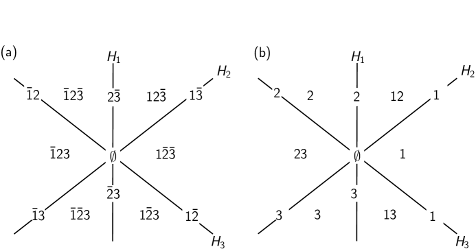
Figure 4: (a) The covectors of an oriented matroid arising from a central hyperplane arrangement. The topes are $\bar{1}2\bar{3},12\bar{3},1\bar{2}\bar{3},1\bar{2}3,\bar{1}\bar{2}3$ and $\bar{1}23$ (b) The combinatorial code of the cover given by the positive open half-spaces.

A central hyperplane arrangement $\mathcal{H}$ divides $\mathbb{R}^{d}$ into a set of polyhedral chambers. The natural labels assigned to these chambers form the covectors of a representable oriented matroid. These labels can be written as sign vectors, i.e. elements of $\{+,-,0\}^{n}$. We can assign each point $x\in\mathbb{R}^{d}$ to a sign vector by

$$X_{i}=\begin{cases}~{}+&\mbox{ if }h^{*}_{i}(x)>0\\ ~{}-&\mbox{ if }h^{*}_{i}(x)<0\\ ~{}0&\mbox{ if }h^{*}_{i}(x)=0.\end{cases}$$

The family $\mathcal{L}(\mathcal{H})$ of sign vectors which arise in this way is known as the set of covectors of the oriented matroid $\mathcal{M}(\mathcal{H})=([n],\mathcal{L}(\mathcal{H}))$. The covectors of top-dimensional cells are called topes of $\mathcal{M}$.

Notice that $\mathcal{L}(\mathcal{H})$ records the same information as $\operatorname{code}(H_{1}^{+},\ldots,H_{n}^{+},H_{1}^{-},\ldots,H_{n}^{-})$. We can clarify this with alternate notation for sign vectors: defining $\pm[n]=[n]\cup\bar{[}n]:=\{1,\ldots,n\}\cup\{\bar{1},\ldots,\bar{n}\}$, we can write the sign vector $X$ as the set $X:=\{i\mid X_{i}=+\}\cup\{\bar{i}\mid X_{i}=-\}$. In this notation,

$$\mathcal{L}(\mathcal{H})=\operatorname{code}(H_{1}^{+},\ldots,H_{n}^{+},H_{1}^{-},\ldots,H_{n}^{-})\subseteq 2^{\pm[n]}.$$

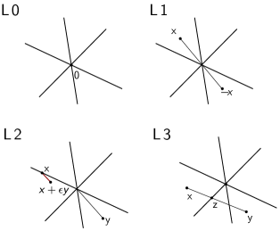
Figure 5: Geometric interpretation of the covector axioms.

The set $\mathcal{L}(\mathcal{H})$ satisfies a list of axioms know as the covector axioms for oriented matroids. Oriented matroids are defined in general via these axioms. In order to state them, we introduce some more notation. The support of a sign vector $X$ is the set $\underline{X}:=\{i\mid X_{i}\neq 0\}$. The positive part of $X$ is $X^{+}:=\{i\mid X_{i}=+\}$ and the negative part is $X^{-}:=\{i\mid X_{i}=-\}$. The composition of sign vectors $X$ and $Y$ is defined component-wise by

$$(X\circ Y)_{i}:=\begin{cases}X_{i}\mbox{ if }X_{i}\neq 0\\ Y_{i}\mbox{ otherwise}.\end{cases}$$

The separator of $X$ and $Y$ is the unsigned set $\operatorname{sep}(X,Y):=\{i\mid X_{i}=-Y_{i}\neq 0\}$.

Definition 0.3.

Let $E$ be a finite set, and $\mathcal{L}\subseteq 2^{\pm E}$ a collection of sign vectors satisfying the following covector axioms:

1. $\varnothing\in\mathcal{L}$

2. $X\in\mathcal{L}$ implies $-X\in\mathcal{L}$.

3. $X,Y\in\mathcal{L}$ implies $X\circ Y\in\mathcal{L}$.

4. If $X,Y\in\mathcal{L}$ and $e\in\operatorname{sep}(X,Y)$, then there exists $Z\in\mathcal{L}$ such that $Z_{e}=0$ and $Z_{f}=(X\circ Y)_{f}=(Y\circ X)_{f}$ for all $f\notin\operatorname{sep}(X,Y)$.

Then, the pair $\mathcal{M}=(E,\mathcal{L})$ is called an oriented matroid, and $\mathcal{L}$ its set of covectors.

For any hyperplane arrangement, $\mathcal{L}(\mathcal{H})$ must satisfy all of the covector axioms, thus the oriented matroid of a hyperplane arrangement is, in fact, an oriented matroid. We give a geometric interpretation of each covector axiom in Figure 5. An oriented matroid $\mathcal{M}$ is representable if there exists a hyperplane arrangement $\mathcal{H}$ such that $\mathcal{M}=\mathcal{M}(\mathcal{H})$. We discuss representability in more detail in Section Representability.

We can view $\mathcal{L}$ as a poset, with the covectors partially ordered by inclusion. By adjoining a top element $\hat{1}$ with $X\leq\hat{1}$ for all $X\in\mathcal{L}$, we can construct the face lattice of the oriented matroid, $\mathcal{L}\cup\{\hat{1}\}$. Notice that in the realizable case, traversing upwards in this face lattice corresponds to moving from a lower dimensional cell to an adjacent cell of one dimension higher. Thus, the height of this poset tracks the dimension of the space. This lets us define the rank of a matroid as

$$\operatorname{rank}(\mathcal{L})=\mathrm{height}\,(\mathcal{L}\cup\hat{1})-2.$$

In the realizable case, $\operatorname{rank}(\mathcal{L}(\mathcal{H}))$ recovers the rank of the matrix whose columns are the normal vectors to the hyperplanes in $\mathcal{H}$.

We can use oriented matroids to describe affine hyperplane arrangements as well. In particular, an affine oriented matroid $(\mathcal{M},g)$ is an oriented matroid together with a distinguished ground set element $g$. We can define the positive covectors of $(\mathcal{M},g)$ as the set $\mathcal{L}_{+}(\mathcal{M},g):=\{X\in\mathcal{L}(\mathcal{M})|X_{g}=+\}$. Notice that if $\mathcal{M}$ is the oriented matroid of $H_{1},\ldots,H_{n},H_{g}$ where $H_{g}$ is the hyperplane $x_{d+1}=0$, and $H_{1},\ldots,H_{n}$ are centralized versions of affine hyperplanes as above, then the positive covectors $\mathcal{L}_{+}(\mathcal{M},g)$ correspond to cells of the affine hyperplane arrangement.

Circuit axioms

There are many equivalent axiomatizations of oriented matroids. The two formulations we use most often throughout this work are the covector axioms (L1)-(L4), stated above, and the circuit axioms (C1)-(C4), which we state here. The circuit axioms most naturally arise when we consider the oriented matroid of a point arrangement, $p_{1},\ldots,p_{n}\in\mathbb{R}^{d}$.

Definition 0.4.

Let $\mathcal{P}=\{p_{1},\ldots,p_{n}\}$ be a point configuration in $\mathbb{R}^{d}$. The sign vector $X$ is a circuit of the oriented matroid $\mathcal{M}(\mathcal{P})$ of $\mathcal{P}$ if $X^{+}$, $X^{-}$ is a minimal Radon partition of $V$. That is,

$$\operatorname{conv}(\{p_{i}\mid i\in X^{+}\})\cap\operatorname{conv}(\{p_{j}\mid j\in X^{-}\})\neq\varnothing,$$

and for all $Y<X$,

$$\operatorname{conv}(\{p_{i}\mid i\in Y^{+}\})\cap\operatorname{conv}(\{p_{j}\mid j\in Y^{-}\})=\varnothing.$$

The minimal Radon partitions of a point arrangement follow a list of rules known as the circuit axioms for oriented matroids. Oriented matroids are defined via these axioms.

Definition 0.5.

Let $E$ be a finite set, and $\mathcal{C}\subseteq 2^{\pm E}$ a collection of signed subsets satisfying the following circuit axioms:

1. $\varnothing\notin\mathcal{C}$.

2. $X\in\mathcal{C}$ implies $-X\in\mathcal{C}$.

3. $X,Y\in\mathcal{C}$ and $\underline{X}\subseteq\underline{Y}$ implies $X=Y$ or $X=-Y$.

4. For all $X,Y\in\mathcal{C}$ with $X\neq-Y$ and an element $e\in X^{+}\cap Y^{-}$, there is a $Z\in\mathcal{C}$ such that $Z^{+}\subseteq(X^{+}\cup Y^{+})\setminus e$ and $Z^{-}\subseteq(X^{-}\cup Y^{-})\setminus e$.

Then the pair $\mathcal{M}=(E,\mathcal{C})$ is an oriented matroid, and $\mathcal{C}$ is its set of circuits.

Note that it is possible to recover the dimension of the affine span of the point arrangement of $\mathcal{C}(\mathcal{P})$ via Radon’s theorem.

In particular, if $\mathcal{C}(\mathcal{P})$ is a point configuration in $\mathbb{R}^{d}$, then every set of at least $d+2$ points contains the support of circuit. Further, as long as all points are not contained in a lower-dimensional subspace, there is at least one set of $d+1$ points which does not contain the support of circuit. Motivated by this, the rank of an oriented matroid is defined as the maximum size of a set $X$ which does not contain the support of a circuit. Note that this means a point arrangement in $\mathbb{R}^{d}$ corresponds to a rank $d+1$ matroid. An oriented matroid is uniform if all of its circuits have the same cardinality. Uniform oriented matroids correspond to point arrangements which are in general position.

Duality

We can translate between the circuit and covector descriptions of an oriented matroid, illustrated in the case of point arrangements in Figure 6. Circuits are related to covectors as follows: Two signed sets $X$ and $Y$ are called orthogonal if either $\underline{X}\cap\underline{Y}=\varnothing$ or if there exist $e,f\in\underline{X}\cap\underline{Y}$ such that $X_{e}X_{f}=-Y_{e}Y_{f}$. A signed set is called a vector of $\mathcal{M}$ if and only if it is orthogonal to every covector. Equivalently, a signed set is a vector of $\mathcal{M}$ if and only if it is orthogonal to every tope. The circuits are the minimal vectors of $\mathcal{M}$, while minimal covectors are called cocircuits. The vectors of an oriented matroid $\mathcal{M}$ are the covectors of its dual oriented matroid $\mathcal{M}^{*}$. Thus, vectors and covectors satisfy the same set of axioms, as do circuits and cocircuits.

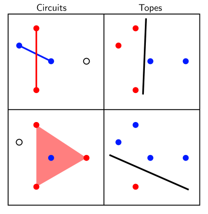
Figure 6: Circuits of an oriented matroid correspond to minimal Radon partitions, while topes correspond to maximal hyperplane partitions.

For a given oriented matroid $\mathcal{M}$, each one of the set of covectors $\mathcal{L}(\mathcal{M})$, the set of topes $\mathcal{W}(\mathcal{M})$, the set of vectors $\mathcal{V}(\mathcal{M})$, and the set of circuits $\mathcal{C}(\mathcal{M})$ is sufficient to recover all of the others.

We can build geometric intuition around duality by considering the oriented matroid of a point arrangement. Let $\mathcal{P}$ be a point arrangement, and note that a signed set $X$ with $\underline{X}=[n]$ is a tope of $\mathcal{M}$ if and only if it is orthogonal to every circuit of $\mathcal{M}$. Then there is no circuit $Y$ of $\mathcal{M}$ such that $Y\subseteq X$. Then $\operatorname{conv}(\{p_{i}\}_{X_{i}=+})\cap\operatorname{conv}(\{p_{j}\}_{X_{j}=-})=\varnothing$. Thus, the topes of the oriented matroid of a point arrangement correspond to the partitions of the set of points which can be achieved with a hyperplane. In general, $X$ is a covector of $\mathcal{M}(\mathcal{P})$ if there exists a hyperplane $H$ such that $X^{+}=\{i\mid p_{i}\in H^{+}\},X^{-}=\{j\mid p_{j}\in H^{-}\},X^{0}=\{k\mid p_{k}\in H\}$.

We can also see duality in the case of hyperplane arrangements through receptive field relationships, similar (but not identical) to those defined via the neural ring in [2]. In particular, suppose $X$ is a circuit of $\mathcal{C}(\mathcal{H})$. Then $X$ is orthogonal to each covector of $\mathcal{L}(\mathcal{H})$. For each point $p$, let $Y(p)$ be the sign vector at the point $p$. Then either $\underline{Y(p)}\cap\underline{X}=\varnothing$, or there exists $j\in Y(P)^{+}\cap X^{-}$, $k\in Y(P)^{-}\cap X^{+}$. In the first case, we have $p\in H_{i}$ for all $i\in\underline{Y}$. In the second case, we have $p\in H_{j}^{+}$ for some $j\in X^{-}$, $p\in H_{k}^{-}$ for some $k\in X^{+}$. Thus, the sets $\{\bar{H}_{j}^{+}\}_{j\in X^{-}}\cup\{\bar{H}_{k}^{-}\}_{j\in X^{+}}$ cover $\mathbb{R}^{d}$. Equivalently, $\bigcap_{j\in X^{+}}H_{j}^{+}\subseteq\bigcup_{k\in X-}\bar{H}_{k}^{+}$.

Representability

An oriented matroid $\mathcal{M}$ is representable if $\mathcal{M}=\mathcal{M}(\mathcal{H})$ for some hyperplane arrangement $\mathcal{H}$, or, equivalently, $\mathcal{M}=\mathcal{M}(\mathcal{P})$ for some point arrangement $\mathcal{P}$. Figure 18(a) illustrates an example in $\mathbb{R}^{2}$. Not every oriented matroid is representable–see Chapter 8 of [40] for more information on represnentability. However, we are able to take this hyperplane picture as paradigmatic. The topological representation theorem guarantees that every oriented matroid has a representation by a pseudosphere arrangement: a collection of centrally symmetric topological $d-2$ spheres embedded in $\mathbb{S}^{d-1}$ whose intersections are also spheres of the appropriate dimension [52]. See Chapter 5 of [40] for more information on the topological representation theorem. See Figure 7 for an illustration. For a representable oriented matroid, we can obtain a representation with a sphere arrangement by intersecting each hyperplane with a sphere containing the origin.

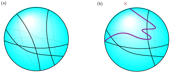
Figure 7: (a) A pseudosphere arrangement (b) Not a pseudosphere arrangement.

In general, it is difficult to determine whether an oriented matroid is representable. In particular, by [24, 25, 26] determining representability is NP-hard. In fact, something stronger is true: determining representability is complete for the existential theory of the reals. This is the complexity class of decision problems of the form

$$\exists(x_{1}\in\mathbb{R})\cdots\exists(x_{n}\in\mathbb{R})P(x_{1},\ldots,x_{n}),$$

where P is a quantifier-free formula whose atomic formulas are polynomial equations and inequalities in the $x_{i}$ [53]. Problems which are $\exists\mathbb{R}$-complete are not believed to be computationally tractable. In particular, they must be NP-hard. Many classic problems in computational geometry fall into $\exists\mathbb{R}$ [54]. In particular, in Chapter Oriented Matroids and Convex Neural Codes, we will show that determining whether a code is convex is $\exists\mathbb{R}$ complete. In Chapter The Geometry of Underlying Rank, we will show that determining the underlying rank of a matrix is $\exists\mathbb{R}$ complete.

There is likely no combinatorial characterization of representability. In particular, focusing on unoriented matroids but with results which apply to oriented matroids as well, a series of papers makes the claim that the “missing axiom of oriented matroid theory is lost forever" [55, 56, 57]. That is, there is no statement in the language of the original matroid axioms which characterizes representable matroids.

Convex Neural Codes

Introduction to Convex Neural Codes

How does the brain keep track of the body’s position in space? In 1948, based on observations that rats in mazes learn the broader geography of the maze, rather than just the correct sequence of turns to reach the goal, Tolman [58] speculated that the brains of rodents (and humans) create and maintain maps of their environments. In 1971 [59], O’Keefe and Dostrovsky recorded the activity of neurons in the hippocampus of a rat which they held on a platform, and found cells which appeared to form part of the cognitive map Tolman posited. In particular, they discovered some neurons which were more active when the rat was at one particular location on the platform, and other neurons which were more active when the rat was oriented in one particular direction. In [1], O’Keefe mapped the receptive fields of cells they named place cells, and found them to be contiguous, roughly convex subsets of the rat’s environment.

From subsequent work, we now know that place cells determine location by integrating input from multiple sensory systems, and by performing path integration based on the animal’s motion [60]. While place cells have one convex firing field within a small environment, place cells have multiple fields in larger environments, with no apparent relationship between the different fields [61]. Over time, place fields within one environment are remapped, i.e. some cells stop being active, others become active, and some have their place fields move. The relationships between place fields change over time. Place cells are part of a larger navigational system, involving grid cells and head direction cells.

Early on, it was observed that it is possible to decode location from the collective activity of place cells [1]. Once technology made it possible to record enough place cells to be possible, this was demonstrated in [62]. However, these decoding mechanisms make use of the encoding map: observations of the locations of the place fields. This is not information that the brain has access to.

In [63], Curto and Itskov asked to what information about the environment can be decoded from place cell activity alone, without information about the locations of place fields. In particular, they use the nerve theorem to show that it is possible to recover the topology of the environment using the sets of place cells which fire together, on the assumption that place cells have convex receptive fields.

A key observation of [63] is that if $U_{1},\ldots,U_{n}$ are interpreted as place fields, $\operatorname{nerve}(\mathcal{U})$ consists of the sets of place cells which fire together. Thus, we can use the nerve theorem to recover the topology of $\bigcup_{i=1}^{n}U_{i}$ from neural activity, even if all we know about the receptive fields is that they are convex.

Convex and non-convex codes

In [2], Curto, Itskov, Veliz-Cuba, and Youngs go beyond the nerve, studying the relationships between receptive fields which are implied by neural activity. In particular, they focus on the the combinatorial neural codes, which record more detail about how receptive fields interact than the nerve of a cover.

Definition 0.6.

A combinatorial neural code is a subset $\mathcal{C}\subseteq 2^{[n]}$. Elements of the code are called codewords.

We interpret the codewords as sets of neurons which fire at roughly the same time, and the neural code as the collection of all sets of neurons which are observed to fire together over some time. While codewords are often written as binary vectors, we use more compact subset notation. For instance, if at some time neuron 1 fires alone, at another time neurons 1 and 2 fire together, and at a third time, neurons 2 and 3 fire together, and at a fourth time no neurons fire, we denote this with the neural code $\mathcal{C}=\{\{1\},\{1,2\},\{2,3\},\varnothing\}$. For compactness, we will omit brackets and commas on the inner sets, abbreviating this as $\mathcal{C}=\{1,12,23,\varnothing\}$.

Given a family of sets $\mathcal{U}$, we can define a combinatorial neural code.

Definition 0.7.

Let $\mathcal{U}=\{U_{1},\ldots,U_{n}\}$ be a collection of subsets of a set $X$. The code of $\mathcal{U}$, written $\operatorname{code}(\mathcal{U})$, is the set

$$\operatorname{code}(\mathcal{U}):=\{\sigma\mid U_{\sigma}\setminus\bigcup_{j\notin\sigma}U_{j}\neq\varnothing\}.$$

We define the atom of a codeword as

$$\mathcal{U}^{\sigma}:=\{U_{\sigma}\setminus\bigcup_{j\notin\sigma}U_{j}\}$$

In cases where the universe $X$ is not clear from context, we will write $\operatorname{code}(\mathcal{U},X)$.

Equivalently, $\operatorname{code}(\mathcal{U})$ is the set of labels which arise when we label each point $p\in X$ with the set of $i$ such that $p\in U_{i}$. See Figure 1 for the relationship between neural activity, combinatorial neural codes, and receptive fields.

We can recover $\operatorname{nerve}(\mathcal{U})$ by completing $\operatorname{code}(\mathcal{U})$ to a simplicial complex.

Definition 0.8.

Let $\mathcal{C}$ be a combinatorial neural code. Define a simplicial complex $\Delta(\mathcal{C})$ as the smallest abstract simplicial complex containing $\mathcal{C}$, i.e. as

$$\Delta(\mathcal{C}):=\{\tau\mid\tau\subseteq\sigma\mbox{ for some }\sigma\in\mathcal{C}\}$$

Notice that

$$\Delta(\mathcal{C}(\mathcal{U}))=\operatorname{nerve}(\mathcal{U}).$$

To what extent does the constraint of having convex receptive fields show up in the structure of the combinatorial code itself? That is, can we characterize which combinatorial codes arise from the activity of neurons with convex receptive fields?

Definition 0.9.

A neural code $\mathcal{C}$ is convex open (resp. closed) if there exists a family of convex open (resp. closed) sets $\mathcal{U}=\{U_{1},\ldots,U_{n}\}$ in $\mathbb{R}^{d}$ such that $\mathcal{C}=\operatorname{code}(\mathcal{U})$. The if $\mathcal{C}$ is convex, the minimum value of $d$ for which this is possible is referred to as the minimal embedding dimension.

Question 0.1.

Can we give an intrinsic characterization of which neural codes are convex? Is there an algorithm to determine whether a code is convex? Can we compute or estimate the minimal embedding dimension of a code?

An answer to Question 0.1 would make it possible to search for convex receptive field geometry in regions of the brain where the receptive fields are less straightforward than those of hippocampal place cells. Additionally, such a characterization would help us to characterize the connectivity of neural circuits which give rise to neurons with convex receptive fields. Finally, Question 0.1 turns out to be mathematically rich, with connections to other work in discrete geometry.

Not every code is convex. For instance, the code $\mathcal{C}=\{12,13\}$ is neither convex open nor convex closed. To see this, suppose to the contrary that there are convex sets $U_{1},U_{2},U_{3}$, either all open or all closed, such that $\mathcal{C}=\operatorname{code}(U_{1},U_{2},U_{3})$. Since neuron $1$ never fires alone, we have $U_{1}=U_{2}\cup U_{3}$. However, neurons 2 and 3 never fire together, so $U_{2}\cap U_{3}=\varnothing$. Thus, $U_{2}$, $U_{3}$ gives a disconnection of $U_{1}$. Since convex sets must be connected, this is a contradiction. This is an example of a local obstruction. Without the assumption that our sets are all open or all closed, it is true that all codes are convex [5], though these constructions are often highly degenerate.

Giusti and Itskov make a first step towards answering Question 0.1 in [64], which characterizes non-convex codes via local obstructions. We use the characterization of local obstructions provided in [4, Theorem 1.3]. We first define the link of a simplex in a simplicial complex.

Definition 0.10.

Let $\Delta$ be a simplicial complex. Then the link of a simplex $\sigma\in\Delta$ is the set

$$\operatorname{link}_{\Delta}(\sigma)=\{\tau\in\Delta\mid\sigma\cap\tau=\varnothing,\sigma\cup\tau\in\Delta\}$$

Definition 0.11.

Let $\mathcal{C}$ be a combinatorial neural code. Then $\mathcal{C}$ has a local obstruction if there is a $\sigma\in\Delta(\mathcal{C})$ such that $\sigma\notin\mathcal{C}$ and $\operatorname{link}_{\Delta(\mathcal{C})}(\sigma)$ is not contractible.

Notice that for each simplicial complex $\Delta$, this defines a minimal code with no local obstructions

$$\mathcal{C}_{\min}(\Delta)=\{\sigma\in\Delta\mid\operatorname{link}_{\Delta(\mathcal{C})}(\sigma)\mbox{ is not contractible }\}$$

If $\sigma$ is not the intersection of facets of $\Delta(\mathcal{C})$, then $\operatorname{link}_{\Delta(\mathcal{C})}(\sigma)$ is automatically contractible. Thus, when checking for local obstructions, we can restrict to codewords $\sigma$ which are intersections of facets, also called maximal codewords. We often write the maximal codewords in bold.

Theorem 0.4 (Theorem 3, [64]).

If $\mathcal{C}$ is convex (either open or closed), it has no local obstructions.

To see this, notice that if $\sigma\in\Delta(\mathcal{C})\setminus\mathcal{C}$, then $U_{\sigma}=\bigcup_{j\notin\sigma}U_{\sigma}\cap U_{j}$. On the assumption that $U_{1},\ldots,U_{n}$ are convex and either all open or all closed, this is a good cover. Also notice that $\operatorname{nerve}(\{U_{\sigma}\cap U_{j}\}_{j\notin\sigma})=\operatorname{link}_{\sigma}(\Delta(\mathcal{C})$. Thus, $\operatorname{link}_{\Delta(\mathcal{C})}(\sigma)$ is homotopy equivalent to $\bigcap_{i\in\sigma}U_{i}$ by the nerve theorem. Thus, if $\mathcal{C}$ is convex, $\sigma\in\Delta(\mathcal{C})\setminus\mathcal{C}$, $\operatorname{link}_{\Delta(\mathcal{C})}(\sigma)$ must be contractible. Notice that we can weaken the requirement that $U_{1},\ldots,U_{n}$ be convex here to a requirement that $U_{1},\ldots,U_{n}$ forms a good cover.

One might hope that the converse of this theorem holds, that a code is convex if and only if it has no local obstructions. Unfortunately, while this is true for codes on at most four neurons, this is not the case in general. In particular, the code

$$\mathcal{C}_{1}=\{{\bf 2345},{\bf 123},{\bf 134},{\bf 145},13,14,23,34,45,3,4,\varnothing\}$$

has no local obstructions, and is closed-convex (Figure 8 (a)), but not open-convex [8]. On the other hand, the code

$$\mathcal{D}_{1}=\{{\bf 123},{\bf 234},{\bf 345},{\bf 145},{\bf 125},12,23,34,45,15,\varnothing\},$$

the has no local obstructions and is open convex (Figure 8 (b)), but is not closed convex. This code first appears in [18], and is a simplified version of a code introduced in [6]. We will give a proof that this code is not convex in Example 0.5 in Chapter Order Forcing in Neural Codes. By combining these two codes in a clever way, [13] gives an eight neuron code which has no local obstructions, but is neither open nor closed convex

$$\mathcal{C}=\{\mathbf{2345},\mathbf{123},\mathbf{124},\mathbf{145},12,14,23,24,45,2,4,\varnothing\}\cup\{\mathbf{237},\mathbf{238},\mathbf{367},\mathbf{678},\mathbf{26},37,67,6,8\}.$$

It is true, however, that $\mathcal{C}$ is a good cover code if and only if it has no local obstructions [7].

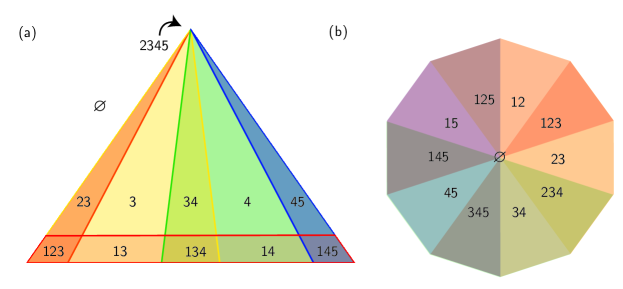
Figure 8: (a) A closed convex realization of $\mathcal{C}_{1}$. (b) An open convex realization of $\mathcal{D}_{1}$.

On the other hand, there are large families of codes which we can guarantee are convex. In particular, we say a code $\mathcal{C}$ is max-intersection complete if whenever $\sigma\in\Delta(\mathcal{C})$ is an intersection of maximal codewords, $\sigma\in\mathcal{C}$. By [6], all max-intersection complete codes are both open and closed convex. Thus, the codes where convexity is an interesting problem are the codes which are not max-intersection complete, but have no local obstructions. We can partially order the set of codes $\mathcal{C}$ with the same simplicial complex $\Delta(\mathcal{C})=\Delta$ by inclusion. Cruz et al. prove that open convexity is monotone increasing under this order [6]. On the other hand, closed convexity is not monotone increasing under this order [13].

On up to four neurons, a code has no local obstructions if and only if it is max intersection complete–thus on up to four neurons, a code is convex if and only if it has no local obstructions. A classification of all codes on at most three neurons appears in [2], while a classification of codes on four neurons appears in [4]. A complete classification of codes on five neurons appears in [18]. In particular, $\mathcal{C}_{1}$ is the only code on five neurons which has no local obstructions, but is not open convex. In addition to $\mathcal{D}_{1}$, there are two other five neurons which are closed, but not open convex:

$$\mathcal{C}_{6} =\{{\bf 125},{\bf 234},{\bf 145},{\bf 123},4,23,15,12,\varnothing\}$$

$$\mathcal{C}_{10} =\{{\bf 134},{\bf 245},{\bf 234},{\bf 135},12,1,5,34,13,2,24,\varnothing\}$$

Codes with at most three maximal codewords are convex if and only if they have no local obstructions, by [19].

By a stronger version of Theorem 0.4 proved in [7], if a code is convex, the simplicial complexes which occur as links of missing codewords must be collapsible, not just contractible. In fact, they must satisfy even stronger properties established in [17]. The complete classification of which simplicial complexes arise as links in convex codes remains open.

Embedding dimensions of open and closed convex codes

Beyond determining whether or not a code is convex, we can characterize its minimal embedding dimension. It turns out that we get different answers asking this question for open, closed, and non-degenerate convex codes.

Definition 0.12.

A collection $\mathcal{U}=\{U_{1},\ldots,U_{n}\}$ of open convex sets is non-degenerate if the collection of their closures $\operatorname{cl}(\mathcal{U})=\{\operatorname{cl}(U_{1}),\ldots,\operatorname{cl}(U_{n})\}$ has code $\operatorname{code}(\mathcal{U})=\operatorname{code}(\operatorname{cl}(\mathcal{U}))$. Likewise, a collection of closed sets $\mathcal{U}=\{U_{1},\ldots,U_{n}\}$ is non-degenerate if the collection of their interiors $\operatorname{int}(\mathcal{U})=\{\operatorname{int}(U_{1}),\ldots,\operatorname{int}(U_{n})\}$ has $\operatorname{code}(\mathcal{U})=\operatorname{code}(\operatorname{int}(\mathcal{U}))$.

The open, closed, and non-degenerate embedding dimensions of a code are defined as follows:

Definition 0.13.

Let $\mathcal{C}$ be a neural code. Then the open, closed, and non-degenerate embedding dimensions of $\mathcal{C}$ are defined, respectively, as

$$\operatorname{odim}(\mathcal{C}) =\min\{d\mid\mathcal{C}\mbox{ has an open realziation in }\mathbb{R}^{d}\}$$

$$\operatorname{cdim}(\mathcal{C}) =\min\{d\mid\mathcal{C}\mbox{ has an closed realziation in }\mathbb{R}^{d}\}$$

$$\operatorname{ndim}(\mathcal{C}) =\min\{d\mid\mathcal{C}\mbox{ has an non-degenerate realziation in }\mathbb{R}^{d}\}$$

First, we note that if $\mathcal{C}$ is convex, then $\operatorname{odim}(\mathcal{C})\leq|\mathcal{C}|-1$, since we can obtain a lower-dimensional realization of $\mathcal{C}$ by intersecting our realization of $\mathcal{C}$ with the affine hull of a set of points $\{p_{\sigma}\}_{\sigma\in\mathcal{C}}$, where $\{p_{\sigma}\}$ is taken to be in the atom of $\sigma$. This result holds for $\operatorname{cdim}(\mathcal{C})$ and $\operatorname{ndim}(\mathcal{C})$ as well. A slightly better bound exists when $\mathcal{C}$ is max-intersection complete: by Theorem 1.2 of [6], $\operatorname{odim}(\mathcal{C}),\operatorname{cdim}(\mathcal{C})\leq\max\{2,k-1\}$ where $k$ is the number of maximal codewords of $\mathcal{C}$. If $\mathcal{C}$ is intersection complete, then $\operatorname{cdim}(\mathcal{C})\leq\min\{2d+1,n-1\}$, where $d$ is the dimension of $\Delta(\mathcal{C})$.

These bounds allow for the possibility that the minimal embedding dimension is exponential in the number of neurons, even for max-intersection complete codes. In fact, this can occur, at least for open embedding dimension: Jeffs [16] gives an infinite family of intersection-complete codes $\mathcal{E}_{n}$, such that $\operatorname{odim}(\mathcal{E}_{n})$ grows as fast as $\frac{2^{n-1}}{n}$. These codes have closed embedding dimension at most $n$, since they are intersection complete. There are no know examples of closed-convex codes on $n$ neurons such that $n<\operatorname{cdim}(\mathcal{C})<\infty$.

As the previous example demonstrates, open and closed embedding dimension can be wildly different. In some cases, we can still control the relationship between $\operatorname{odim}(\mathcal{C}),\operatorname{cdim}(\mathcal{C})$, and $\operatorname{ndim}(\mathcal{C})$. For instance, if any one of $\operatorname{odim}(\mathcal{C}),\operatorname{cdim}(\mathcal{C})$,or $\operatorname{ndim}(\mathcal{C})$ is equal to 1, then the other two embedding dimensions must be 1. If $\mathcal{C}$ is a simplicial complex, then $\operatorname{odim}(\mathcal{C})=\operatorname{cdim}(\mathcal{C})$, and if $\mathcal{C}$ is intersection complete, then $\operatorname{cdim}(\mathcal{C})\leq\operatorname{odim}(\mathcal{C})$. Other than this, the only constraint on the open, closed, and non-degenerate embedding dimensions of a code is the clear constraint that the non-degenerate embedding dimension must be at least the maximum of the closed and open embedding dimensions. That is, any triple $(a,b,c)$ such that $a,b\leq c$ and $2\leq a,b,c$, there is a code $\mathcal{C}$ with $\operatorname{odim}(\mathcal{C})=a,\operatorname{cdim}(\mathcal{C})=b$, and $\operatorname{ndim}(\mathcal{C})=c$ [15].

Morphisms of neural codes

Across all of mathematics, objects make more sense when we can relate them to one another. Combinatorial codes are no exception. In order to describe the relationships between codes, Jeffs introduces neural code morphisms in [10]. These maps between codes allow us to relate the convexity of one code to the convexity of another, or even the convexity of one class of codes to another class of codes. In particular, they allow give us a formal way to talk about whether non-convex code is novel, rather than a trivial modification of a previous code.

Morphisms of neural codes are defined in terms of trunks.

Definition 0.14.

Let $\mathcal{C}$ be a neural code. The trunk of $\sigma\in\mathcal{C}$ is the set

$$\operatorname{trunk}_{\mathcal{C}}(\sigma):=\{\tau\in\mathcal{C}\mid\sigma\subseteq\tau\}$$

A subset of $\mathcal{C}$ is a trunk if it is empty, or if it is equal to $\operatorname{trunk}_{\mathcal{C}}(\sigma)$ for some $\sigma\subseteq[n]$.

Definition 0.15.

Let $\mathcal{C}$, $\mathcal{D}$ be combinatorial neural codes. A map $f:\mathcal{C}\to\mathcal{D}$ is a morphism of neural codes if the preimage of every trunk of $\mathcal{D}$ is a trunk of $\mathcal{C}$. Two codes $\mathcal{C}$ and $\mathcal{D}$ are isomorphic if there is a bijective code morphism $f:\mathcal{C}\to\mathcal{D}$ whose inverse is also a code morphism.

Note that while this definition feels reminiscent of the definition of a continuous map between topological spaces, the trunks of a code need not form the open sets of a topology on $\mathcal{C}$. In particular, the union of trunks need not be a trunk.

A key property of code morphisms is that the preserve convexity.

Theorem 0.5 (Theorem 1.3, [10]).

If $\mathcal{C}$ is a convex code, and $f:\mathcal{C}\to\mathcal{D}$ is a surjective map, then $\mathcal{D}$ is a convex code.

This fact motivates Jeffs to define a partial order on codes such that convex codes are a down-set. If there is a sequence of codes $\mathcal{C}=\mathcal{C}_{0},\mathcal{C}_{1},\dots,\mathcal{C}_{k}=\mathcal{D}$ such that each successive code is either the image of a morphism from or a trunk of the preceding code, we say $\mathcal{D}$ is a minor of $\mathcal{C}$. Codes are then quasi-ordered by setting $\mathcal{D}\leq\mathcal{C}$ if $\mathcal{D}$ is a minor of $\mathcal{C}$. The poset of isomorphism classes of codes induced by this order is denoted $P_{\operatorname{code}}$. We can then rephrase Theorem 0.5 as the statement that the set of convex codes in $P_{\operatorname{code}}$ is downward closed.

The proof of Theorem 0.5 is constructive, allowing us to build a realization of $\mathcal{D}$ out of the realization of $\mathcal{C}$. To see this, we first use Proposition 2.11 of [10], which says that all code morphisms take a certain form.

Proposition 0.1 (Proposition 2.11, [10]).

Let $\mathcal{C}$ be a neural code, $S=\{T_{1},\ldots,T_{m}\}$ a finite collection of trunks of $\mathcal{C}$. Define the function $f_{S}:\mathcal{C}\to 2^{[m]}$ by

$$f_{S}(\sigma)=\{i\mid\sigma\in T_{i}\}.$$

We say that $f_{S}$ is the morphism determined by the trunks in $S$. The map $f_{S}$ is indeed a code morphism. Further, every code morphism is of this form.

Jeffs uses this fact prove Theorem 1.3 constructively. In fact, the only property of convex sets his proof uses is that the intersection of convex sets is convex. Thus, in [11], Kunin, Rosen and I generalize this result to intersection-closed families, of which the family of open convex subsets of $\mathbb{R}^{d}$ is one example. In particular, this allows us to show that codes with no local obstructions form a down-set in $P_{\operatorname{code}}$. We include this argument here.

A family $\mathcal{F}$ of subsets of a topological space is called intersection-closed if it is closed under finite intersections and contains the empty set. We say that a neural code $\mathcal{C}$ is $\mathcal{F}$-realizable if $\mathcal{C}=\operatorname{code}(\mathcal{U},X)$ for some $\mathcal{U}\subseteq\mathcal{F}$ and $X\in\mathcal{F}$. For instance, a neural code is convex if and only if it is $\mathcal{F}$-realizable for the set $\mathcal{F}$ of convex open subsets of some $\mathbb{R}^{d}$.

Lemma 0.1.

For any intersection closed family $\mathcal{F}$, if $\mathcal{C}$ is $\mathcal{F}$-realizable and $\mathcal{D}\leq\mathcal{C}$, then $\mathcal{D}$ is $\mathcal{F}$-realizable.

Proof.

This closely follows the proof of Theorem 1.4 in [10], since the only property of convex sets this proof uses is that the family of open convex subsets of $\mathbb{R}^{d}$ is closed under finite intersection. . We repeat the details here. Let $\mathcal{C}\subseteq 2^{[n]}$, $\mathcal{D}\subseteq 2^{[m]}$. Since $\mathcal{D}\leq\mathcal{C}$, we have $\mathcal{D}=f(\mathcal{C})$. By Proposition 0.1, there are trunks $T_{1},\ldots,T_{m}$ in $\mathcal{C}$ that define the morphism $f:\mathcal{C}\to\mathcal{D}$. Let $\{U_{1},\ldots,U_{n}\}\subseteq\mathcal{F}$ be an $\mathcal{F}$-realization of $\mathcal{C}$.

If $T_{j}$ is nonempty, let $\sigma_{j}$ be the unique largest subset of $[n]$ such that $T_{j}=\operatorname{trunk}_{\mathcal{C}}(\sigma_{j})$. In particular, $\sigma_{j}$ will be the intersection of all elements of $T_{j}$. Then, for $j\in[m]$, define

$$V_{j}=\begin{cases}\varnothing&T_{j}=\varnothing\\ \bigcap_{i\in\sigma_{j}}U_{i}&T_{j}\neq\varnothing\end{cases}$$

Since $\mathcal{F}$ is closed under finite intersection and contains the empty set, $V_{j}\in\mathcal{F}$ for all $j\in[m]$. Thus, it suffices to show that the code $\mathcal{E}$ that they realize is $\mathcal{D}$. To see this, note that we can associate each point $p\in X$ to a codeword in $\mathcal{C}$ or $\mathcal{E}$ by $p\mapsto\{i\in[n]\mid p\in U_{i}\}$ and $p\mapsto\{j\in[m]\mid p\in V_{j}\}$. Then let $p\in X$ be arbitrary, and let $c$ and $e$ be the associated codewords in $\mathcal{C}$ and $\mathcal{E}$ respectively. Observe that by the definition of the $V_{j}$, we have that $c\in T_{j}$ if and only if $j\in e$. But this is equivalent to $e=f(c)$. Since $p$ was arbitrary and every codeword arises at some point, we conclude that $\mathcal{E}=f(\mathcal{C})=\mathcal{D}$, as desired.

An example of this construction is illustrated in Figure 9.

∎

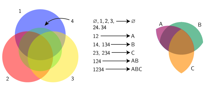
Figure 9: Example of construction from proof of Lemma 0.1.

To prove Theorem 0.5, we apply Lemma 0.1 to the intersection closed family of open or closed convex sets in $\mathbb{R}^{d}$. We also show that codes with no local obstructions form a down-set in $P_{\operatorname{code}}$. The only requirement to be an open set in some good cover is contractibility, and the family of contractible sets is not intersection-closed. Instead, we consider the sets $U_{1},\ldots,U_{n}$ in one particular good cover and their intersections as our intersection-closed family.

Corollary 0.1.

The set of codes with no local obstructions is a down-set in $P_{\operatorname{code}}$.

Proof.

Let $\mathcal{C}$ be a code with no local obstructions, $\mathcal{D}\leq\mathcal{C}$. By [7, Theorem 3.13], $\mathcal{C}$ is a good cover code. Fix a good cover $\mathcal{U}=\{U_{1},\ldots,U_{n}\}$ realizing $\mathcal{C}$. Let $\mathcal{F}_{\mathcal{U}}$ denote the family of sets obtained by arbitrary intersections of sets in $\mathcal{U}$, together with the empty set. This family still forms a good cover. $\mathcal{D}$ lies below $\mathcal{C}$ and is therefore $\mathcal{F}_{\mathcal{U}}$-realizable by 0.1; it is therefore a good cover code and thus has no local obstructions. ∎

Using the structure provided by $P_{\operatorname{code}}$, Jeffs defines minimally non-convex codes: a code $\mathcal{C}$ is minimally non-convex if it is not convex, but all codes $\mathcal{C}^{\prime}$ such that $\mathcal{C}^{\prime}\leq\mathcal{C}$ are convex. Using this framework, Jeffs constructs a minimally non-convex code $\mathcal{C}^{\prime}$ on six neurons by taking images of the code $\mathcal{C}_{1}$ from [8].

We can produce infinitely many distinct non-convex codes by (for instance) adding new neurons to the code $\mathcal{C}$ from [8]. A more interesting question is whether or not there are infinitely many minimal non-convex codes. In contrast to case for graphs, where any minor-closed family has finitely many excluded minors by the famous result of Robertson and Seymour, there are infinitely many minimally non-convex codes. In particular, there is a minimal non-convex code corresponding to each non-collapsible simplicial complex by Proposition 5.8 of [10].

A more explicit infinite family of minimally non-convex codes generalizing $\mathcal{C}_{1}$ is given in [9]. This family depends on the following fact about sunflowers of convex open sets, proved in the same paper. Say $\mathcal{U}=\{U_{1},\ldots,U_{n}\}$ is a sunflower if for any $i,j$, $U_{i}\cap U_{j}=\bigcap_{i=1}^{n}U_{i}$. The intersection $U=\bigcap_{i=1}^{n}U_{i}$ is referred to as the center of the sunflower.

Theorem 0.6 (Theorem 1.1, [9]).

Let $\mathcal{U}=\{U_{1},\ldots,U_{n},U_{d+1}\}$ be a sunflower of $d+1$ convex opens sets in $\mathbb{R}^{d}$. Then any hyperplane which intersects each $U_{i}$ must also intersect the center $\bigcap_{i=1}^{n}U_{i}$.

We can construct non-convex codes by forcing a hyperplane to intersect each of the $U_{i}$, but not the center. In Chapter Order Forcing in Neural Codes, we provide an alternate family of minimally non-convex codes with no local obstructions generalizing $\mathcal{C}_{1}$ which uses only the $n=3$ case of the sunflower theorem.

Order Forcing in Neural Codes

This chapter is adapted from the paper “Order Forcing in Neural Codes", which is joint work with Amzi Jeffs and Nora Youngs [27], and is included here with their permission.

Introduction

The arguments that the codes $\mathcal{C}_{1}$ and $\mathcal{D}_{1}$ in Section Convex and non-convex codes are not convex share a common feature: at some step, they derive a contradiction by showing that any convex realization would have a straight line path passing through a certain sequence of atoms in a certain order. In this chapter, we introduce a combinatorial concept that we call order-forcing which allows us to generalize these arguments. Order-forcing provides an elementary connection between the combinatorics of a code and the geometric arrangement of atoms in its open or closed realizations. In particular, our main result is the following:

Theorem 0.1.

Let $\sigma_{1},\sigma_{2},\ldots,\sigma_{k}$ be an order-forced sequence of codewords in a code $\mathcal{C}\subseteq 2^{[n]}$. Let $\mathcal{U}=\{U_{1},\ldots,U_{n}\}$ be a (closed or open) convex realization of $\mathcal{C}$, and let $x\in A^{\mathcal{U}}_{\sigma_{1}}$, and $y\in A^{\mathcal{U}}_{\sigma_{k}}$. Then the line segment $\overline{xy}$ must pass through the atoms of $\sigma_{1},\sigma_{2},\ldots,\sigma_{k}$, in this order.

We will use order-forcing to construct new examples of non-convex codes. In Section Order-Forcing, we define an order-forced sequence of codewords and prove Theorem 0.7. In Section New Examples of Non-Convex Codes we use order-forcing to describe new good cover codes that are not convex:

• We generalize a minimally non-convex code from [10] based on sunflowers of convex open sets to a family $\{\mathcal{L}_{n}\mid n\geq 0\}$ of minimally non-convex good cover codes (Proposition 0.2).

• We build a good cover code $\mathcal{R}$ that is neither open nor closed convex by using order-forcing to guarantee that two disjoint sets would cross one another in a convex realization of $\mathcal{R}$ (Proposition 0.3). This example is notable in that it relies on the order that codewords appear along line segments, rather than just certain codewords being “between" one another.

• We build a good cover code $\mathcal{T}$ that is neither open nor closed convex by using order-forcing to guarantee a non-convex “twisting" in every realization of $\mathcal{T}$ (Proposition 0.4).

These examples illustrate the utility of order-forcing. The codes $\mathcal{T}$ and $\mathcal{R}$ have the advantage that they require only elementary geometric techniques (i.e. order-forcing) to analyze. The codes $\mathcal{T}$ and $\mathcal{R}$ are also the first “natural" examples we know of of good cover codes which are not produced by combining a non-open-convex code and a non-closed-convex code.

Order-Forcing

When we constrain ourselves to realizations that use only open (or only closed) convex regions $U_{i}$, we restrict not only which codes may be realized, but how regions in these realizations can be arranged. In particular, when we move along continuous paths through realizations composed of open (or closed) sets $U_{i}$, we are limited in the transitions we can make from one atom to the next.

Lemma 0.2.

Suppose $\mathcal{C}\subseteq 2^{[n]}$ is a neural code with a good cover realization $\mathcal{U}$, and let $\sigma$ and $\tau$ be codewords of $\mathcal{C}$. If there are points $p_{\sigma}\in A^{\mathcal{U}}_{\sigma}$ and $p_{\tau}\in A^{\mathcal{U}}_{\tau}$ and a continuous path from $p_{\sigma}$ to $p_{\tau}$ that is contained in $A^{\mathcal{U}}_{\sigma}\cup A^{\mathcal{U}}_{\tau}$ (that is, if the atoms are adjacent in the realization), then either $\sigma\subseteq\tau$ or $\tau\subseteq\sigma$.

Proof.

Let $P$ be the image of a continuous path from $p_{\sigma}$ to $p_{\tau}$ with $P\subseteq A^{\mathcal{U}}_{\sigma}\cup A^{\mathcal{U}}_{\tau}$. Suppose for contradiction that $\sigma\not\subset\tau$ and $\tau\not\subset\sigma$. Then there exist elements $i\in\sigma\setminus\tau$ and $j\in\tau\setminus\sigma$. But then $U_{i}\cap P$ and $U_{j}\cap P$ partition $P$ (every point in $P$ is in exactly one of $A_{\sigma}^{\mathcal{U}}$ or $A_{\tau}^{\mathcal{U}}$ and thus in exactly one of $U_{i}$ or $U_{j}$). Since our good cover consists of sets that are all open or all closed, the sets $U_{i}\cap P$ and $U_{j}\cap P$ are both relatively open or both relatively closed in $P$. This contradicts the fact that $P$ is connected, so $\sigma\subseteq\tau$ or $\tau\subseteq\sigma$ as desired. ∎

Thus, as we move continuously through any good cover realization of a code, we are moving along edges in the following graph $G_{\mathcal{C}}$:

Definition 0.16.

Let $\mathcal{C}\subseteq 2^{[n]}$ be a neural code. The codeword containment graph of $\mathcal{C}$ is the graph $G_{\mathcal{C}}$ whose vertices are codewords of $\mathcal{C}$, with edges $\{\sigma,\tau\}$ when either $\sigma\subsetneq\tau$ or $\tau\subsetneq\sigma$. Note that this graph is also defined in [14].

Example 0.1.

Consider the code $\mathcal{C}=\{{\bf 1235},{\bf 1245},{\bf 1256},125,13,14,15,\varnothing\}$. The graph $G_{\mathcal{C}}$ for this code is shown in Figure 10.

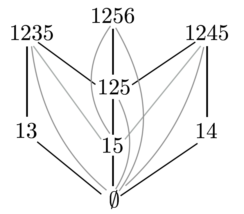
Figure 10: The codeword containment graph $G_{\mathcal{C}}$ for the code in Example 0.1.

Lemma 0.2 implies that any continuous path from one codeword region to another codeword region in an open (or closed) realization of the code $\mathcal{C}$ must correspond to a walk in the graph $G_{\mathcal{C}}$. For straight-line paths within a convex realization, this walk must respect convexity, a property we call feasibility (see Lemma 0.3).

Definition 0.17.

Let $\mathcal{C}$ be a neural code and $G_{\mathcal{C}}$ its codeword containment graph. A $\sigma,\tau$ walk $\sigma=v_{1},v_{2},...,v_{k}=\tau$ in $G_{\mathcal{C}}$ is called feasible if $v_{i}\cap v_{j}\subseteq v_{m}$ for all $1\leq i<m<j\leq k$.

In general, if there exists a feasible $\sigma,\tau$ walk, then by removing portions of the walk between repeated vertices, we can obtain a feasible $\sigma,\tau$ path. This does not, however, mean that there is a corresponding straight line path in the realization which would follow precisely this sequence of codewords. For example, one could form a closed realization of the code $\{\mathbf{1},\mathbf{2},\mathbf{3},\varnothing\}$ in which $U_{2}$ is a hyperplane, and $U_{1}$ and $U_{3}$ are contained in its positive and negative side respectively. Then any straight line from the atom of $1$ to the atom of $3$ must pass through the atom of 2, but the path $1,\varnothing,3$ is a feasible path in $G_{\mathcal{C}}$ regardless.

Example 0.2 (Example 0.1 continued).

Consider the codewords $\sigma=13$ and $\tau=14$ in $\mathcal{C}$ from the code in Example 0.1. There are many $\sigma,\tau$ walks; however, not all are feasible. For example, the walk $13,1235,15,1245,14$ would not be feasible; however, the walk $13,1235,125,1275,125,1245$ is a feasible $\sigma,\tau$ walk. This walk contains the feasible path $13,1235,125,1245,14$, which in this case is the unique feasible $\sigma,\tau$ path.

Lemma 0.3.

Suppose $\mathcal{C}\subseteq 2^{[n]}$ is a neural code with a convex realization $\mathcal{U}=\{U_{1},\ldots,U_{n}\}$, and let $\sigma$ and $\tau$ be codewords of $\mathcal{C}$. If there are points $p_{\sigma}\in A^{\mathcal{U}}_{\sigma}$ and $p_{\tau}\in A^{\mathcal{U}}_{\tau}$, then the sequence of atoms along the line $\overline{p_{\sigma}p_{\tau}}$ forms a feasible walk in $G_{\mathcal{C}}$.

Proof.

Select points $p_{\sigma}\in A^{\mathcal{U}}_{\sigma}$ and $p_{\tau}\in A^{\mathcal{U}}_{\tau}$, and let the sequence of atoms along the line be given by $\sigma=\tau_{1},\tau_{2},...,\tau_{\ell}=\tau$. By Lemma 0.2, if we cross directly from $A_{\tau_{i}}^{\mathcal{U}}$ to $A_{\tau_{i+1}}^{\mathcal{U}}$ along the path $\overline{xy}$, then either $\tau_{i}\subseteq\tau_{i+1}$ or $\tau_{i+1}\subseteq\tau_{i}$, thus $(\tau_{i},\tau_{i+1})$ is an edge of $G_{\mathcal{C}}$. Thus, $\tau_{1},\ldots,\tau_{\ell}$ is a walk in $G_{\mathcal{C}}$. To check feasibility, we need to show that for all $i\leq j\leq k$, $\tau_{i}\cap\tau_{k}\subseteq\tau_{j}$. We can choose points $x_{i},x_{j}$, and $x_{j}$ in this order along $\overline{p_{\sigma}p_{\tau}}$ such that $x_{i}\in A_{\tau_{i}}^{\mathcal{U}}$, $x_{j}\in A_{\tau_{j}}^{\mathcal{U}}$, $x_{k}\in A_{\tau_{k}}^{\mathcal{U}}$. Since $\{U_{1},\ldots,U_{n}\}$ is a convex realization and intersections of convex sets are convex, $U_{\tau_{i}\cap\tau_{k}}$ is a convex set. By the definition of a convex set, the line segment $\overline{x_{i}x_{k}}$ is contained in $U_{\tau_{i}\cap\tau_{k}}$. Thus, $x_{j}\in U_{\tau_{i}\cap\tau_{k}}$, so $\tau_{i}\cap\tau_{k}\subseteq\tau_{j}$. Thus, $\tau_{1},\ldots,\tau_{\ell}$ is a feasible walk.

∎

The idea of feasibility gives us a new tool for finding possible obstructions to convexity. In any convex realization of a code, straight line paths between points in the same set $U_{i}$ must correspond to feasible walks in the graph, and so codes where feasible walks are rare or nonexistent can force us into contradictions. To that end, we define a few particular restrictions we will encounter.

Definition 0.18.

Let $\mathcal{C}$ be a neural code and $G_{\mathcal{C}}$ its codeword containment graph. We say a vertex $v$ of $G_{\mathcal{C}}$ is forced between vertices $\sigma$ and $\tau$ if every feasible $\sigma,\tau$ path passes through $v$.

Example 0.3 (Example 0.1 continued).

In the codeword containment graph $G_{\mathcal{C}}$, we see that $1245$ is forced between $14$ and $15$. There are many possible feasible paths from $14$ to $15$ (for example (14, 1245, 15) or (14, 1245, 125, 15) or (14, 1245,125, 1235, 15), but all these paths must use $1245$.

In cases where there are multiple codewords forced between two vertices of our graph, we often find that these vertices are also forced into a particular order, a situation we call order-forcing.

Definition 0.19.

Let $\mathcal{C}$ be a neural code and $G_{\mathcal{C}}$ its corresponding graph. A sequence of codewords $\sigma_{1},...,\sigma_{k}$ is order-forced if every feasible $\sigma_{1},\sigma_{k}$ path contains these codewords as a subsequence.

Definition 0.20.

Let $\mathcal{C}$ be a neural code and $G_{\mathcal{C}}$ its corresponding graph. A feasible path $\sigma_{1},...,\sigma_{k}$ is strongly order-forced if $\sigma_{1},...,\sigma_{k}$ is the unique feasible $\sigma_{1},\sigma_{k}$ walk in $G_{\mathcal{C}}$.

Example 0.4.

Consider the code

$$\mathcal{C}=\{{\bf 2456},{\bf 123},{\bf 145},{\bf 437},{\bf 467},45,46,47,1,2,3,\varnothing\}$$

In this code, the sequence $145,45,2456,46,467,47,473$ is strongly order-forced. In order to have a path in $G_{\mathcal{C}}$ from $145$ to $437$ which is feasible, we can certainly only use codewords which contain $4$. If we restrict to the portion of $G_{\mathcal{C}}$ which contains $4$, we have that this subgraph is a path with endpoints $145$ and $437$. Thus, there is a unique path from $145$ to $437$, and we can check that this path is feasible.

Theorem 0.7.

Let $\sigma_{1},\sigma_{2},\ldots,\sigma_{k}$ be an order-forced sequence of codewords in a code $\mathcal{C}\subseteq 2^{[n]}$. Let $\mathcal{U}=\{U_{1},\ldots,U_{n}\}$ be a (closed or open) convex realization of $\mathcal{C}$, and let $x\in A^{\mathcal{U}}_{\sigma_{1}}$, and $y\in A^{\mathcal{U}}_{\sigma_{k}}$. Then the line segment $\overline{xy}$ must pass through the atoms of $\sigma_{1},\sigma_{2},\ldots,\sigma_{k}$, in this order.

Proof.

Let $\sigma_{1},\ldots,\sigma_{k}$ be an order-forced sequence in a code $\mathcal{C}.$ Let $\mathcal{U}=\{U_{1},\ldots,U_{n}\}$ be a (closed or open) convex realization of $\mathcal{C}$. Let $x\in A_{\sigma_{1}}^{\mathcal{U}}$ and $y\in A_{\sigma_{k}}^{\mathcal{U}},$ and let $\overline{xy}$ be the line segment from $x$ to $y$. Let $\tau_{1}=\sigma_{1},\tau_{2},\ldots,\tau_{\ell}=\sigma_{k}$ be the sequence of atoms along $\overline{xy}$. By Lemma 0.3, we have that $\tau_{1},\ldots,\tau_{\ell}$ is a feasible walk from $\sigma_{1}$ to $\sigma_{k}$ in $G_{\mathcal{C}}.$ Since every feasible walk from $\sigma_{1}$ to $\sigma_{k}$ contains a feasible path from $\sigma_{1}$ to $\sigma_{k}$, and every feasible path from $\sigma_{1}$ to $\sigma_{k}$ contains $\sigma_{1},\sigma_{2},\ldots,\sigma_{k}$ as a subsequence, this suffices to prove Theorem 0.7.

∎

The situation where a codeword $v$ is forced between $\sigma$ and $\tau$ is a special case of order-forcing, and in this case we obtain the following result. Once we know that a sequence is order-forced in a code $\mathcal{C}$, we are often able to obtain several instances of order-forcing.

Corollary 0.2.

Let $\mathcal{C}\subseteq 2^{[n]}$ and suppose $\mathcal{U}=\{U_{1},\ldots,U_{n}\}$ is a (closed or open) convex realization of a code $\mathcal{C}$. If $v\in\mathcal{C}$ is forced between $\sigma$ and $\tau$, then for any $x\in A^{\mathcal{U}}_{\sigma}$, and $y\in A^{\mathcal{U}}_{\tau}$, the line segment $\overline{xy}$ must pass through the atom of $v$.

In the following example, we illustrate the value of these ideas by showing a proof that a relatively small code is open-convex but not closed-convex.

Example 0.5.

We revisit the code $\mathcal{D}_{1}$ from Chapter Introduction to Convex Neural Codes, which was first introduced in [6]. This code is open convex, but not closed convex. This example (in particular the proof that it has no closed convex realization) is an instance of order-forcing, though it was not described by that name in [6]. A slightly smaller example of a similar code which is closed convex, but not open convex appears as code C15 in [18]. In this example, we give a proof of this result which resembles the proof in [6, Lemma 2.9], but is written to make the use of order-forcing explicit.

The code

$$\mathcal{D}_{1}=\{{\bf 123},{\bf 234},{\bf 345},{\bf 145},{\bf 125},12,23,34,45,15,\varnothing\}$$

has an open convex realization, but does not have a closed convex realization.

We have already provided an open-convex realization of $\mathcal{D}_{1}$ in Figure 8 (b).

To show that no closed convex realization may exist, we proceed by contradiction. Suppose that for some $d\geq 1$, there exists a closed convex realization $\{U_{1},\ldots,U_{5}\}$ of $\mathcal{C}$ in $\mathbb{R}^{d}$. Select points $p_{125}\in U_{125}$ and $p_{345}\in U_{345}$. Since both points are within the convex set $U_{5}$, the line segment $L_{1}$ from $p_{125}$ to $p_{345}$ is contained within $U_{5}$. Thus, it cannot pass through $U_{123}$. Note that $U_{123}$ is a closed set, as $123$ is a maximal codeword. Pick a point $p_{123}\in U_{123}$ which minimizes the distance to the set $L_{1}$; this is possible as these sets are disjoint and $L_{1}$ is compact.

Now, consider the line segment $L_{2}$ from $p_{125}$ to $p_{123}$; note that $L_{2}\subset U_{12}$. In this code, $12$ is forced between $125$ and $123$, so by Corollary 0.2 there exists a point $p_{12}$, between $p_{125}$ and $p_{123}$ along this line, which is in $A^{\mathcal{U}}_{12}$. Likewise, if we consider the line segment $L_{3}$ from $p_{123}$ to $p_{345}$, the order-forced sequence $123,23,234,34,345$ implies there is a point $p_{234}\in U_{234}$ on $L_{3}$ which is between $p_{123}$ and $p_{345}$.

Finally, consider the line segment $L_{4}$ between $p_{12}$ and $p_{234}$. $L_{4}$ must pass through $U_{123}$ somewhere between these points because $123$ is forced between $12$ and ${234}$. Select a point $q_{123}$ on this line and within $U_{123}$; then, $q_{123}$ will be closer to $L_{1}$ than $p_{123}$, a contradiction.

New Examples of Non-Convex Codes

In this section, we demonstrate the power of order-forcing by using order-forcing to construct a new infinite family of minimally non-convex codes and two new non-convex codes.

Stretching sunflowers

Early examples of good cover codes which are not convex come from the sunflower theorem, Theorem 0.6. The $d=2$ case of this theorem was used as a lemma to give the first example of a non-convex good cover code in [8, Theorem 3.1]. In this section, we give a new infinite family of non-convex codes generalizing this code. In order to produce further examples of non-convex codes, we need a notion of what it means for a new code to be genuinely different from an old one. For instance, it is easy to produce “new" non-convex codes by relabeling neurons, or by adding more neurons in some trivial way.

In this subsection, we introduce a family of codes $\{\mathcal{L}_{n}\mid n\geq 0\}$ which generalize $\mathcal{C}_{0}$ to an infinite family of minimally non-convex codes. Geometrically, each of these codes is only a small modification of the code $\mathcal{C}_{0}$, and has the same basic obstruction to convexity. This lies in contrast to [9, Theorem 4.2], which generalizes the non-convex code $\mathcal{C}_{0}$ in [10, Theorem 5.10] to an infinite family of minimally non-convex codes by using higher-dimensional versions of the sunflower theorem. Thus the family $\{\mathcal{L}_{n}\mid n\geq 0\}$ demonstrates that the intuition that each minimally non-convex code should result from a “new" obstruction to convexity does not hold.

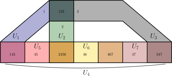
Figure 11: $\mathcal{L}_{1}=\{\mathbf{2456},\mathbf{123},\mathbf{145},\mathbf{437},\mathbf{467},45,46,47,1,2,3,\varnothing\}$

Definition 0.21.

For $n\geq 0$, define the code

$$\mathcal{L}_{n}=\{\varnothing,1,2,3,\mathbf{123},\mathbf{145},45,\mathbf{2456},46,\mathbf{467},47,\mathbf{478},\ldots,4(n+6),34(n+6)\}.$$

For instance, $\mathcal{L}_{1}=\{\mathbf{2456},\mathbf{123},\mathbf{145},\mathbf{437},\mathbf{467},45,46,47,1,2,3,\varnothing\}$. A good cover realization of $\mathcal{L}_{1}$ is given in Figure 11.

Notice below that $\mathcal{L}_{0}$ is equal to $\mathcal{C}_{0}$ under the permutation of the neurons $2\leftrightarrow 3$ and $4\leftrightarrow 5$. Thus, the family $\mathcal{L}_{n}$ generalizes $\mathcal{C}_{0}$. Even though each $\mathcal{L}_{n}$ is minimally non-convex, the non-convexity of $\mathcal{L}_{0}$ directly implies the non-convexity of each $\mathcal{L}_{n}$ for $n>0$.

Proposition 0.2.

For $n\geq 0$, the code $\mathcal{L}_{n}$ is a good cover code, but is minimally non-convex.

Proof.

We first show that $\mathcal{L}_{n}$ is non-convex by induction on $n$. The base case, that $\mathcal{L}_{0}$ is non-convex, is proven by [10, Theorem 5.10] since $\mathcal{L}_{0}$ is permutation equivalent to the code $\mathcal{C}_{0}$ in this paper. Now, we show that if $\mathcal{L}_{n-1}$ is not convex, then neither is $\mathcal{L}_{n}$. We do this by proving the contrapositive: in any convex realization of $\mathcal{L}_{n}$, we can merge the sets $U_{n+5}$ and $U_{n+6}$ in a convex realization of $\mathcal{L}_{n}$ to produce a convex realization of $\mathcal{L}_{n-1}$. That is, if $\{U_{1},\ldots,U_{n+5},U_{n+6}\}$ is a convex realization of $\mathcal{L}_{n}$, then $\{V_{1},\ldots,V_{n+5}\}$ is a convex realization of $\mathcal{L}_{n-1}$ where $V_{1}=U_{1},\ldots,V_{n+4}=U_{n+4},V_{n+5}=U_{n+5}\cup U_{n+6}$.

This gives us two things to check. First, we must check that $\operatorname{code}(\{V_{1},\ldots,V_{n+5}\})=\mathcal{L}_{n-1}$. If $\sigma$ is a codeword of $\mathcal{L}_{n}=\operatorname{code}(\{U_{1},\ldots,U_{n+6}\})$ which does not contain the neuron $n+6$, then $\sigma$ is still a codeword of $\operatorname{code}(\{V_{1},\ldots,V_{n+5}\})$. The three codewords of $\mathcal{L}_{n}$ which contain $n+6$ are $4(n+5)(n+6)$, $4(n+6)$, and $34(n+6)$. If we pick a point $p$ in the atom of $4(n+5)(n+6)$ or $4(n+6)$ with respect to $U_{1},\ldots,U_{n}$, it is now in the atom of $4(n+5)$. If we pick a point in the atom of $34(n+6)$ with respect to $U_{1},\ldots,U_{n+6}$, it is in the atom of $34(n+5)$ with respect to $\{V_{1},\ldots,V_{n+6}\}$.

Next, we must check that $V_{5}=U_{n+5}\cup U_{n+6}$ is convex. That is, we must check that for each pair of points $x,y\in U_{n+5}\cup U_{n+6}$, the line segment from $x$ to $y$ is contained in $U_{n+5}\cup U_{n+6}$. Without loss of generality, let $x\in U_{n+5}\setminus U_{n+6}$, $y\in U_{n+6}\setminus U_{n+5}$. The point $x$ must be contained in the atom of $4(n+5)$ or $4(n+5)(n+4)$. (If $n=1$, $4(n+5)(n+4)$ replaces with $24(n+5)(n+4)$.) The point $y$ must be contained in the atom of $4(n+6)$ or $34(n+6)$. In all of these cases, the only feasible path from $x$ to $y$ in $G_{\mathcal{L}_{n}}$ includes only codewords containing $n+5$ or $n+6$:

$$4(n+5)\leftrightarrow 4(n+5)(n+6)\leftrightarrow 4(n+6)\leftrightarrow 34(n+6).$$

Thus the line segment from $x$ to $y$ is contained in $U_{n+6}\cup U_{n+6}$. See Figure 12 for an illustration of this argument.

To show that $\mathcal{L}_{n}$ is minimally nonconvex, we must show that all codes covered by $\mathcal{L}_{n}$ in the poset $P_{\operatorname{code}}$ are convex. We give a proof of this in Appendix Constructions of Various Realizations, Construction 0.1. ∎

Our proof uses ideas similar to the idea of a rigid structure in Section 4 of [14]. In particular, our argument that $U_{n+5}\cup U_{n+6}$ must be convex is essentially an open-convex version of a rigid structure, which is a subset of neurons whose union must be convex in any closed-convex realization of a code.

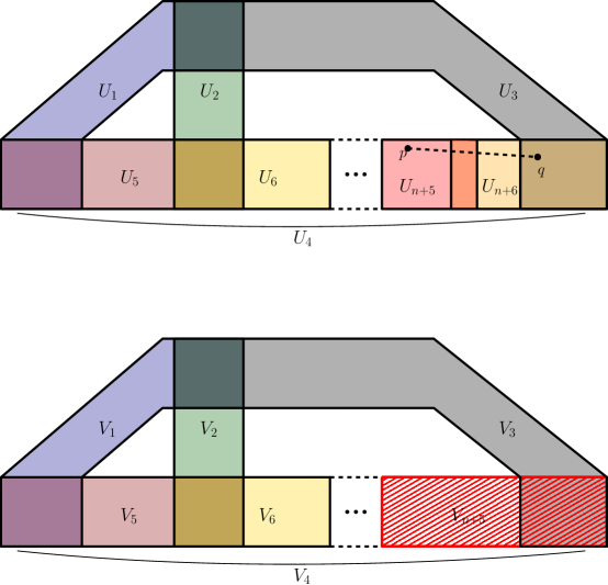
Figure 12: A sketch of the proof of Proposition 0.2. Since the union of $U_{n+5}$ and $U_{n+6}$ is forced to be convex, we can use a realization of $\mathcal{L}_{n}$ to construct a realization of $\mathcal{L}_{n-1}$.

Simple proofs of nonconvexity

In this section, we give two new examples of good cover codes which are neither open nor closed convex. The proofs that these codes are not convex depend only on order-forcing and elementary geometric arguments. Below, we use lowercase letters for neurons where it would be cumbersome to use only integers.

Figure 13: A good-cover realization of the non-convex code $\mathcal{R}$ in $\mathbb{R}^{3}$. The open sets $U_{a},U_{b},U_{c},U_{d},U_{e},U_{f},U_{g},U_{h},U_{i},U_{j}$ are not shown. Instead, maximal order-forced codewords are noted with vertices, and sets of order-forced vertices are indicated with dashed lines.

Proposition 0.3.

The code

$$\mathcal{R} =\{\mathbf{12ab},\mathbf{13ace},\mathbf{14ch},\mathbf{23bgd},\mathbf{24dj},\mathbf{35ef},\mathbf{36fg},\mathbf{46hi},\mathbf{45ij},$$

$$\quad\quad 1a,1c,2b,2d,3e,3f,3g,4i,4h,4j,5,6,\varnothing\}$$

is a good cover code, but is neither open nor closed convex.

Proof.

We first show that if $\mathcal{R}$ is convex, then it has a convex realization in the plane. We then show that it does not. Choose points $p_{12}\in A_{12ab}^{\mathcal{U}}$, $p_{14}\in A_{14ch}^{\mathcal{U}}$, and $p_{24}\in A_{24dj}^{\mathcal{U}}$. We will use order-forcing to show that each atom of any realization of $\mathcal{R}$ must have nonempty intersection with $A=\operatorname{conv}(p_{12},p_{14},p_{24})$, so that $\{U_{i}\cap A\mid i\in\{1,\ldots,6,a,\ldots,h\}\}$ is a convex realization of $\mathcal{R}$ in $\mathrm{aff}(p_{12},p_{14},p_{24})\cong\mathbb{R}^{2}$.

First, notice the following order-forced sequences:

1. the only feasible path from $12ab$ to $14ch$ is

   $$12ab\leftrightarrow 1a\leftrightarrow 13ace\leftrightarrow 1c\leftrightarrow 14ch$$

2. the only feasible path from $12ab$ to $24dj$ is

   $$12ab\leftrightarrow 2b\leftrightarrow 23bdg\leftrightarrow 2d\leftrightarrow 24dj$$

3. the only feasible path from $14ch$ to $24dj$is

   $$14ch\leftrightarrow 4h\leftrightarrow 46hi\leftrightarrow 45ij\leftrightarrow 4j\leftrightarrow 24dj$$

4. the only feasible path from $13ace$ to $23bgd$ is

   $$13ace\leftrightarrow 3e\leftrightarrow 35ef\leftrightarrow 3f\leftrightarrow 36fg\leftrightarrow 3g\leftrightarrow 23bgd$$

5. the only feasible path from $35ef$ to $45ij$ is

   $$35ef\leftrightarrow 5\leftrightarrow 45ij$$

6. the only feasible path from $36fg$ to $46hi$ is

   $$36fg\leftrightarrow 6\leftrightarrow 46hi.$$

Now, by Theorem 0.7 and order-forcings (1), (2), and (4), the atoms corresponding to codewords

$$\{12ab,1a,13ace,1c,14ch,2b,23bdg,2d,24dj,4h,46hi,45ij,4j\}$$

have nonempty intersection with $A$. Thus, we can pick $p_{13}\in A\cap A_{13ace}^{\mathcal{U}}$, $p_{23}\in A\cap A_{23bdg}^{\mathcal{U}}$, $p_{45}\in A\cap A_{45ij}^{\mathcal{U}}$, and $p_{46}\in A\cap A_{46hi}^{\mathcal{U}}$. Applying order-forcing (3) to $p_{13}$ and $p_{23}$, we deduce that the atoms corresponding to codewords

$$\{3e,35ef,3f,36fg,3g\}$$

have nonempty intersection with $A$. Thus, we can pick $p_{35}\in A\cap A_{35ef}^{\mathcal{U}}$ and $p_{36}\in A\cap A_{36fg}^{\mathcal{U}}$. Finally, applying order-forcings (5) and (6), we deduce that the atoms corresponding to codewords $\{5,6\}$ have nonempty intersection with $A$. This accounts for all codewords of $\mathcal{R}$.

Next, we show that $\mathcal{R}$ cannot have a realization in the plane. Note that by applying an appropriate affine transformation, we can assume that $p_{12}$ is above $p_{14}$ and $p_{24}$, with $p_{14}$ to the left of $p_{24}$, as pictured in Figure 13. Then by order-forcings (3) and (4), $p_{35}$ must be to the left of $p_{36}$, while $p_{45}$ must be to the right of $p_{46}$. This implies the line segments $\overline{p_{35}p_{45}}$ and $\overline{p_{36}p_{46}}$ must intersect. But if $p\in\overline{p_{35}p_{45}}\cap\overline{p_{36}p_{46}}$, then $p\in U_{5}\cap U_{6}$. But, since $U_{5}$ and $U_{6}$ must be disjoint in any realization of $\mathcal{R}$, this is not possible. ∎

Proposition 0.4.

The code

$$\mathcal{T}=\{\mathbf{14a},\mathbf{15ab},\mathbf{16bg},\mathbf{25c},\mathbf{24cd},\mathbf{26dgh},\mathbf{34e},\mathbf{35ef},\mathbf{36fh},$$

$$1a,1b,2c,2d,3e,3f,6g,6h,4,5,\varnothing\}$$

is a good cover code, but is neither closed nor open convex.

Figure 14: A good cover realization of the code $\mathcal{T}$.

Proof.

Suppose to the contrary that $\mathcal{T}$ has a convex realization $\{U_{1},\ldots,U_{6},U_{a},\ldots,U_{h}\}$. Since the sets $U_{4}$ and $U_{5}$ must be disjoint convex sets which are either both open or both closed, there exists a hyperplane $H$ separating them. In particular, if $U_{4}$ and $U_{5}$ are both open, then by the open-set version of the hyperplane separation theorem there is a hyperplane strictly separates them. That is, $H$ separates $\mathbb{R}^{n}$ into open half spaces $H^{+}$ and $H^{-}$ with $U_{4}\subseteq H^{+}$ and $U_{5}\subseteq H^{-}$. This also holds if $U_{4}$ and $U_{5}$ are both closed. In this case, then without loss of generality, we can choose both sets to be compact. Thus by the compact-set version of the separating hyperplane theorem, there exists a hyperplane $H$ strictly separating them. We will use order-forcing to exhibit a line segment which crosses $H$ twice, a contradiction.

We show that the triples of codewords corresponding to marked points in Figure 14 are order-forced. More specifically, we have that:

1. the only feasible path from $14a$ to $16bg$ is

   $$14a\leftrightarrow 1a\leftrightarrow 15ab\leftrightarrow 1b\leftrightarrow 16bg$$

2. the only feasible path from $25c$ to $26dgh$ is

   $$25c\leftrightarrow 2c\leftrightarrow 24cd\leftrightarrow 2d\leftrightarrow 26dgh$$

3. the only feasible path from $34e$ to $36fh$ is

   $$34e\leftrightarrow 3e\leftrightarrow 35ef\leftrightarrow 3f\leftrightarrow 36fh$$

4. the only feasible path from $16bg$ to $36fh$ is

   $$16bg\leftrightarrow 6g\leftrightarrow 26dgh\leftrightarrow 6h\leftrightarrow 36fh.$$

Choose points $p_{14}\in U_{14a}$, $p_{16}\in U_{16bg}$,$p_{25}\in U_{25c}$, $p_{34}\in U_{34e}$, and $p_{36}\in U_{36fh}$. Define line segments $L_{1}=\overline{p_{14}p_{16}}$ and $L_{3}=\overline{p_{34}p_{36}}$. Notice that by order-forcing (1) we may choose $p_{15}\in L_{1}\cap U_{15ab}$. Similarly by order-forcing (3) we may choose $p_{35}\in L_{3}\cap U_{35ef}$.

By ordering forcing (4) we may choose a point $p_{26}\in U_{26dgh}$ on the line segment $\overline{p_{16}p_{36}}$. Lastly, order-forcing (2) allows us to choose a point $p_{24}\in U_{24cd}$ on the line segment $L_{2}=\overline{p_{25}p_{26}}$.

Since each of $L_{1}$ and $L_{3}$ can only cross $H$ once, the fact that $p_{14}$ and $p_{34}$ are contained in $U_{4}$, and thus in $H^{+}$ implies that the points $p_{16}$ and $p_{36}$ are contained in $H^{-}$. Likewise, the fact that $L_{2}$ crosses $H$ only once and $p_{25}$ is contained in $U_{5}$, and thus in $H^{+}$, implies that the point $p_{26}$ is contained in $H^{-}$. Thus, the line from $p_{16}$ to $p_{36}$ crosses $H$ twice, a contradiction. ∎

Note that both of these codes can be used to generate infinite families of non-convex codes using the same trick we use to produce $\mathcal{L}_{n}$ from $\mathcal{L}_{0}$. The codes $\mathcal{T}$ and $\mathcal{R}$ do not lie above any previously known non-convex codes in $P_{\operatorname{code}}$, and in fact are minimally non-convex. This can be checked by exhaustive search of the codes that they cover in $P_{\operatorname{code}}$, as described in Definition 0.22.

Conclusion and Open Questions

Past work constructing non-convex codes has used notions that are similar to, but distinct from, order-forcing. For example, sunflower theorems such as [9, Theorem 1.1] and [16, Theorem 1.11] were used to show that the convex hull of points sampled from certain atoms in a convex realization must intersect another atom. Likewise, [17] used collapses of simplicial complexes to prove that in certain codes the convex hull of appropriately chosen points must intersect certain atoms.

Order-forcing brings a new perspective to this general approach: not only must certain atoms appear, but they must appear in a certain arrangement (i.e. in a particular order along a line segment). The order of points on a line may be generalized to higher dimensions by examining the “order type" of a point configuration [39]. We thus ask the following.

Question 0.2.

Does there exist a general result connecting the combinatorial structure of a code $\mathcal{C}$ to the order type of points chosen from certain atoms in any convex realization of $\mathcal{C}$? Can such a result be formulated so that the connections between convex codes and sunflower theorems [9, 16], convex union representable complexes [17], or oriented matroids [11] are special cases?

A cleanly formulated answer to Question 0.2 would allow us to create fundamentally new families of non-convex codes.

To connect the combinatorics of order-forcing with the geometry of convex realizations, we examined straight line segments between different atoms. One could try to replace convex realizations by good cover realizations, and straight lines by continuous paths, which leads to the following question.

Question 0.3.

If $\mathcal{C}$ is a good cover code, are there feasible paths between all pairs of codewords in $\mathcal{C}$?

Our examples have used order-forcing to prove that codes are not convex. However, even if a code is convex, one might hope to use order-forcing to bound its open or closed embedding dimension.

Question 0.4.

Can one use order-forcing to provide new lower bounds on the open or closed embedding dimension of codes?

Morphisms and minors of codes have played a role in characterizing “minimal" obstructions to convexity, contextualizing results, and systematizing the study of convex codes [10, 16]. It would be interesting to phrase our results in this framework.

Question 0.5.

How does order-forcing interact with code morphisms and minors? If $f:\mathcal{C}\to\mathcal{D}$ is a morphism, and $\sigma_{1},\sigma_{2},\ldots,\sigma_{k}$ is an order-forced sequence in $\mathcal{C}$, under what conditions is $f(\sigma_{1}),f(\sigma_{2}),\ldots,f(\sigma_{k})$ order-forced in $\mathcal{D}$? Similarly, if $f$ is surjective and $\tau_{1},\tau_{2},\ldots,\tau_{k}$ is order-forced in $\mathcal{D}$, when can we find $\sigma_{1},\ldots,\sigma_{k}$ order-forced in $\mathcal{C}$ with $f(\sigma_{i})=\tau_{i}$ (i.e., when can we “pull back" an order-forced sequence)?

Work in [11] used minors of codes to tie the study of convex codes to the study of oriented matroids, in particular showing that non-convex codes come in two types: those that are minors of non-representable oriented matroid codes, and those that are not minors of any oriented matroid code. Concretely, it would be useful to understand which of these classes our codes $\mathcal{T}$ and $\mathcal{R}$ fall into.

Question 0.6.

Are the codes $\mathcal{T}$ and $\mathcal{R}$ from Section New Examples of Non-Convex Codes minors of oriented matroid codes?

Constructions of Various Realizations

Construction 0.1.

In order to check that $\mathcal{L}_{n}$ is minimally non-convex for all $n$, we must show that all codes covered by $\mathcal{L}_{n}$ in $P_{\operatorname{code}}$ are convex. For this, we need the following characterization, from [9], of the covering relations in $P_{\operatorname{code}}$.

Definition 0.22 (Definition 3.9 of [9]).

Let $\mathcal{C}\subseteq 2^{[n]}$ be a code, let $i\in[n]$, and let $\sigma=[n]\setminus\{i\}$. Consider the morphism $f_{i}:\mathcal{C}\to 2^{\sigma\cup\overline{\sigma}}$ defined by

$$f(c)=\begin{cases}c\cap\sigma&i\notin c,\\ c\cap\sigma\cup(\overline{c\cap\sigma})&i\in c.\end{cases}$$

The $i$-th covered code of $\mathcal{C}$ is the image of $\mathcal{C}$ under $f_{i}$, and is denoted $\mathcal{C}^{(i)}$.

Importantly, if a code $\mathcal{D}$ is covered by $\mathcal{C}$ in $P_{\operatorname{code}}$, then $\mathcal{D}$ must be one of the covered codes described above. Thus to prove that a non-convex code $\mathcal{C}$ is minimally non-convex, it suffices to prove that all of its covered codes are convex.

A useful geometric interpretation of covered codes is as follows. Suppose that $\mathcal{U}=\{U_{1},\ldots,U_{n}\}$ is a (possibly not convex) realization of $\mathcal{C}$. Then we may obtain a realization of $\mathcal{C}^{(i)}$ by deleting $U_{i}$ from $\mathcal{U}$, and adding sets $U_{\overline{j}}=U_{i}\cap U_{j}$ for all $j\neq i$.

In some cases, there may be distinct neurons $j,k$ such that $U_{\bar{j}}=U_{\bar{k}}$. In this cases, one of the neurons $\bar{j},\bar{k}$ is redundant, and we can remove it from the code without discarding geometric information. More generally, a neuron $j$ is redundant to a set $\sigma\subseteq[n]\setminus\{j\}$ if $\operatorname{trunk}_{\mathcal{C}}(j)=\operatorname{trunk}_{\mathcal{C}}(\sigma)$, and a neuron is trivial if it does not appear in any codeword [10]. A code is reduced if it does not have any trivial or redundant neurons. Theorem 1.4 of [10] states that a code is always isomorphic to a reduced code. Thus, convexity of the reduced code is equivalent to convexity of the original code. Thus, we can “clean up" $\mathcal{C}^{(i)}$ by removing all trivial or redundant neurons. In what follows, we give realizations for reduced versions of all codes mentioned.

Thus, to show that $\mathcal{L}_{n}$ is minimal for all $n$, we need to construct realizations for each covered code $\mathcal{L}_{n}^{(i)}$. In Figure 15, we construct realizations of $\mathcal{L}_{n}^{(1)}$, $\mathcal{L}_{n}^{(2)}$, and $\mathcal{L}_{n}^{(3)}$ in $\mathbb{R}^{2}$. In Figure 16, we construct a realization of $\mathcal{L}_{n}^{(4)}$ in $\mathbb{R}^{3}$. Finally, in Figure 17, we construct a convex realization of $\mathcal{L}_{n}^{(7)}$ in $\mathbb{R}^{3}.$ An analogous process can be used to construct convex realizations of $\mathcal{L}_{n}^{(8)},\ldots,\mathcal{L}_{n}^{(n+6)}.$

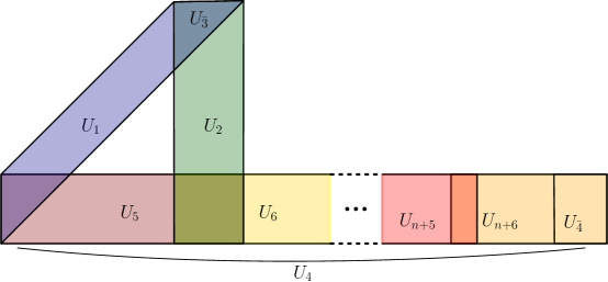
Figure 15: Convex realizations in $\mathbb{R}^{2}$ of the codes $\mathcal{L}_{n}^{(1)}$, $\mathcal{L}_{n}^{(2)}$, $\mathcal{L}_{n}^{(3)}$.

Figure 16: A convex realization in $\mathbb{R}^{3}$ of the code $\mathcal{L}_{n}^{(7)}$. An analogous construction can be used to construct convex realizations for $\mathcal{L}_{n}^{(5)}$, $\mathcal{L}_{n}^{(6)}$, and $\mathcal{L}_{n}^{(8)},\ldots,\mathcal{L}_{n}^{(n+6)}$ in $\mathbb{R}^{3}$.

Figure 17: A convex realization in $\mathbb{R}^{3}$ of the code $\mathcal{L}_{n}^{(7)}$. An analogous construction can be used to construct convex realizations for $\mathcal{L}_{n}^{(5)}$, $\mathcal{L}_{n}^{(6)}$, and $\mathcal{L}_{n}^{(8)},\ldots,\mathcal{L}_{n}^{(n+6)}$ in $\mathbb{R}^{3}$.

Oriented Matroids and Convex Neural Codes

This chapter is adapted from the paper “Oriented Matroids and Convex Neural Codes", which is joint work with Alexander Kunin and Zvi Rosen [11], and is included here with their permission.

Introduction

A convex neural code records the same information about the intersection pattern of a family of convex sets as a representable oriented matroid records about a hyperplane arrangement. For instance, the hyperplane arrangement in Figure 18 gives rise to the covectors illustrated in Figure 18(a), while the codewords of the associated combinatorial code of the positive half-spaces are shown in panel (b). In fact, as we noted in Section Oriented Matroids, the set of covectors of the oriented matroid of a hyperplane arrangement is the code of the positive and negative half-spaces. Thus, we can consider (representable) oriented matroids as a special case of convex neural codes. Because the study of oriented matroids long precedes the study of convex neural codes, making the connection between oriented matroids and convex codes explicit will allow us to leverage results about oriented matroids to prove new theorems about convex codes.

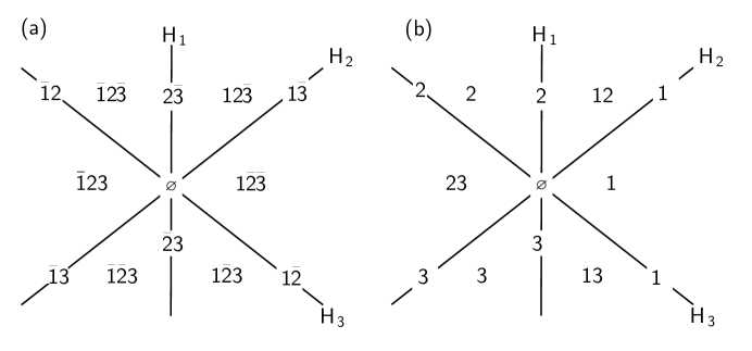
Figure 18: (a) The covectors of an oriented matroid arising from a central hyperplane arrangement. (b) The combinatorial code of the cover given by the positive open half-spaces.

We define a map $\mathsf{L}^{+}$ which takes an oriented matroid to the set of positive parts of its covectors. Using this map, the connection between oriented matroids and convex codes comes primarily through the following theorem, which roughly holds that oriented matroids form the “upper boundary" of the set of convex neural codes in the poset $P_{\operatorname{code}}$.

Theorem 0.1.

A code $\mathcal{C}$ has a realization with convex polytopes if and only if there is an oriented matroid $\mathcal{M}$ such that $\mathcal{C}$ lies below $\mathsf{L}^{+}(\mathcal{M})$ in the poset $P_{\operatorname{code}}$.

This allows us to categorize non-convex codes: if a code is not convex, then either it does not lie below any oriented matroid in $P_{\operatorname{code}}$, or it lies below non-representable matroids only. However, it is not yet known whether every convex code has a realization with convex polytopes. If this does hold, then Theorem 0.1 would give a full characterization of convex codes in terms of representable oriented matroids.

There are many known examples of non-convex codes [4, 8, 10, 9, 7], and we show that many of these fall into the first category: they are non-convex because they are not below any oriented matroids in $P_{\operatorname{code}}$. For instance, codes with topological local obstructions do not lie below oriented matroids. Furthermore, well known examples of non-convex codes with no local obstructions also do not lie below oriented matroids.

Theorem 0.2.

The non-convex codes with no local obstructions introduced in [10, 9] and [8] do not lie below the set of covectors of an oriented matroid in $P_{\operatorname{code}}$.

We are also able to generate an infinite family of non-convex codes of the second kind, those which lie below non-representable matroids only. In order to obtain this family, we establish a relationship between representability and convexity. We do this for the special case of uniform oriented matroids of rank 3, which correspond to non-degenerate pseudoline arrangements in the plane. This construction makes use of order-forcing results from the previous chapter.

Theorem 0.3.

Let $\mathcal{M}$ be a uniform, rank 3 oriented matroid. Then we can construct a code which is convex if and only if $\mathcal{M}$ is representable.

Using this last result, we are able to compare two fundamental decision problems: (1) is a given oriented matroid representable, and (2) is a given neural code realizable by convex sets. We demonstrate that deciding convexity for arbitrary neural codes is at least as hard as deciding representability of an oriented matroid. The latter problem is known to be NP-hard and $\exists\mathbb{R}$-hard, leading to the following theorem:

Theorem 0.4.

The convex code decision problem is NP-hard and $\exists\mathbb{R}$-hard.

The paper is organized as follows: In Section Relating convex codes to oriented matroids, we define the map $\mathsf{L}^{+}$ and prove Theorem 0.1. In Section Non-convex codes, we discuss classes of non-convex codes and their relationships to oriented matroids, proving Theorems 0.2, 0.3, and 0.4. Finally, in Section Open questions, we present open questions related to each area discussed in the paper.

Relating convex codes to oriented matroids

In this section, we establish the relationship between representable oriented matroids and convex neural codes, as well as between oriented matroids and good cover codes.

While the set of covectors of an oriented matroid, viewed as a subset of $2^{\pm[n]}$, is a combinatorial code, it often makes sense to consider a more compact code using only the positive parts of covectors. We define this code as

$$\mathsf{L}^{+}(\mathcal{M})=\{X^{+}\subseteq[n]\mid X\in\mathcal{L}(\mathcal{M})\}$$

In the case that $\mathcal{M}$ is realized by a hyperplane arrangement $H_{1},\ldots,H_{n}$, $\mathsf{L}^{+}(\mathcal{M})$ corresponds to the code of the positive open half-spaces $H_{1}^{+},\ldots,H_{n}^{+}$. Thus, we refer to $\mathsf{L}^{+}(\mathcal{M})$ as the open code of $\mathcal{M}$.

We can also define the closed code of $\mathcal{M}$ via the map $\mathsf{L}^{\geq}(\mathcal{M})$ which takes a representable oriented matroid to the code of its closed positive half-spaces. We do this by taking the complement of the negative part of each covector.

$$\mathsf{L}^{\geq}(\mathcal{M})=\{[n]\setminus X^{-}\mid X\in\mathcal{L}(\mathcal{M})\}$$

Notice that there is not a one-to-one relationship between covectors of an oriented matroid and codewords of $\mathsf{L}^{+}(\mathcal{M})$ or $\mathsf{L}^{\geq}(\mathcal{M})$: multiple covectors may have the same positive part or the same negative part. For instance, in Figure 18, the covectors $\bar{1}2\bar{3}$ and $\bar{1}2$ both have the same positive part, $2$. More significantly, neither $\mathsf{L}^{+}(\mathcal{M})$ nor $\mathsf{L}^{-}(\mathcal{M})$ is an injective map from the set of oriented matroids to the set of convex codes. For example, see Figure 19 for an example of two oriented matroids which map to the same code under $\mathsf{L}^{+}$.

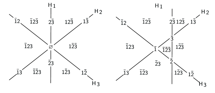
Figure 19: Affine pieces of two oriented matroids which map to the same code. These arrangement can be centralized by adding a fourth hyperplane.

We can also apply $\mathsf{L}^{+}$ and $\mathsf{L}^{\geq}$ to an affine oriented matroid $(\mathcal{M},g)$. In this case, we have

$$\mathsf{L}^{+}(\mathcal{M},g) =\{X^{+}\mid X\in\mathcal{L}_{+}(\mathcal{M},g)\}$$

$$\mathsf{L}^{\geq}(\mathcal{M},g) =\{[n]\setminus X^{-}\mid X\in\mathcal{L}_{+}(\mathcal{M},g)\}.$$

In the representable case, $\mathsf{L}^{+}(\mathcal{M},g)$ is the code of the open half spaces of the affine hyperplane arrangement realizing $(\mathcal{M},g)$ and $\mathsf{L}^{\geq}(\mathcal{M},g)$ is the code of the closed half spaces of the affine hyperplane arrangement realizing $(\mathcal{M},g)$.

We can relate the open code of an affine oriented matroid to the open code of its oriented matroid via trunks. Notice that

$$\mathsf{L}^{+}(\mathcal{M},g)=\operatorname{trunk}_{\mathsf{L}^{+}(\mathcal{M})}(g).$$

However, no such relationship holds in the closed case, since $\operatorname{trunk}_{\mathsf{L}^{\geq}(\mathcal{M})}(g)$ contains codewords whose atoms lie on $H_{g}$, while $\mathsf{L}^{\geq}(\mathcal{M},g)$ does not. In fact, notice that for any oriented matroid, $\mathsf{L}^{\geq}(\mathcal{M})$ contains the full support codeword $[n]$, which is contained in every trunk.

Using Theorem 0.1, we can prove relationships between open convex codes and codes of the form $\mathsf{L}^{+}(\mathcal{M})$, and between closed convex codes and codes of the form $\mathsf{L}^{\geq}(\mathcal{M},g)$. We say that a code $\mathcal{C}$ is open polytope convex if there exists a collection of interiors of convex polytopes $\mathcal{P}=\{P_{1},\ldots,P_{n}\}$ and a bounding convex polytope $X$ such that $\mathcal{C}=\operatorname{code}(\mathcal{P},X)$. Likewise, we say that a code is closed polytope convex if there exists a collection of closed of convex polytopes $\mathcal{P}=\{P_{1},\ldots,P_{n}\}$ and a bounding convex polytope $X$ such that $\mathcal{C}=\operatorname{code}(\mathcal{P},X)$.

Notice that both the set of interiors of convex polytopes and the set of convex closed polytopes are intersection-closed. Thus, Theorem 0.1 implies that the image of any open (closed) polytope code under a surjective morphism is also an open (closed) polytope code. Thus, a code $\mathcal{C}$ is open polytope convex if $\mathcal{C}\leq\mathsf{L}^{+}(\mathcal{M})$ and is closed polytope convex if $\mathcal{C}\leq\mathsf{L}^{\geq}(\mathcal{M},g)$ for some representable oriented matroid $\mathcal{M}$. We prove the converse, showing that every polytope code is itself the image of the code of an oriented matroid under some surjective morphism. This demonstrates that polytope codes are a down-set whose “upper boundary" is the set of representable oriented matroid codes.

Theorem 0.1.

A code $\mathcal{C}$ is open polytope convex if and only if there exists a representable oriented matroid $\mathcal{M}$ such that $\mathcal{C}\leq\mathsf{L}^{+}(\mathcal{M})$.

A code $\mathcal{C}$ is closed polytope convex if and only if there exists a representable affine oriented matroid $(\mathcal{M},g)$ such that $\mathcal{C}\leq\mathsf{L}^{\geq}(\mathcal{M},g)$.

Proof.

($\Rightarrow$) Note that if $\mathcal{M}$ is a representable (affine) oriented matroid, then $\mathsf{L}^{+}(\mathcal{M})$ and $\mathsf{L}^{+}(\mathcal{M},g)$ can be realized with open half-spaces, and $\mathsf{L}^{\geq}(\mathcal{M})$ and $\mathsf{L}^{\geq}(\mathcal{M},g)$ can be realized with closed half-spaces. Then by Theorem 0.1, any code $\mathcal{C}\leq\mathsf{L}^{+}(\mathcal{M})$ or $\mathcal{C}\leq\mathsf{L}^{+}(\mathcal{M},g)$ has a realization with intersections of open half-spaces, i.e. open convex polytopes, and any code $\mathcal{C}\leq\mathsf{L}^{\geq}(\mathcal{M})$ or $\mathcal{C}\leq\mathsf{L}^{\geq}(\mathcal{M},g)$ has a realization with intersections of closed half-spaces, i.e closed convex polytopes.

($\Leftarrow$) Let $\mathcal{C}$ be a polytope convex code with $(\mathcal{V},X)$ a realization of $\mathcal{C}$ with open (closed) convex polytopes $V_{i}$ and bounding convex set $X$. Without loss of generality, we can choose $X$ to be a convex polytope (the convex hull of one point in each atom). Then each $V_{i}$ is the intersection of a collection of open (closed) half spaces $H_{i1}^{+},\ldots,H_{ik_{i}}^{+}$, and $X$ is the intersection of open half spaces $K_{1}^{+},\ldots,K_{k}^{+}$. Now, let $\mathcal{H}=\operatorname{code}(H_{i1}^{+},\ldots,H_{ik_{i}}^{+},\ldots,K_{1}^{+},\ldots,K_{k}^{+}.\},\mathbb{R}^{d})$. Notice that in the open case, $\mathcal{H}=\mathsf{L}^{+}(\mathcal{M},g)$ and in the closed case, $\mathcal{H}=\mathsf{L}^{\geq}(\mathcal{M},g)$ for some representable affine oriented $(\mathcal{M},g)$. Let $\mathcal{H}^{\prime}$ be the trunk of the neurons associated to $K_{1}^{+},\ldots,K_{k}^{+}$.

Now, we define a surjective morphism $f:\mathcal{H}^{\prime}\to\mathcal{C}$ as follows. Choose trunks $T_{1},\ldots,T_{n}$ of $\mathcal{H}^{\prime}$ by $T_{i}=\operatorname{trunk}_{\mathcal{H}^{\prime}}(\{i1,\dots,ik_{i}\})$. Let $f$ be the morphism defined by the trunks $T_{1},\ldots,T_{n}$. We now show that its image is $\mathcal{C}$.

To do this, construct the realization of $f(\mathcal{H}^{\prime})$ given in the proof of 0.1. This construction gives the realization

$$V_{j}^{\prime}=\bigcap_{i=1}^{i=k_{j}}U_{ji}$$

relative to the convex set $X=\bigcap_{i=1}^{k}X_{i}$. Thus, $f(\mathcal{H}^{\prime})=\operatorname{code}(\{V_{1},\ldots,V_{n}\},X)=\mathcal{C}$. Thus, we have shown that any open (closed) polytope convex code lies below the open (closed) polytope convex code of an affine oriented matroid in $P_{\operatorname{code}}$. Further, in the open case, the code of an affine oriented matroid $(\mathcal{M},g)$ is a trunk of the code of the oriented matroid $\mathcal{M}$. Thus, any convex open polytope code lies below the open code of an oriented matroid in $P_{\operatorname{code}}$. ∎

For the remained of this chapter, we focus on open convex codes and $\mathsf{L}^{+}(\mathcal{M})$. We begin by noting that codes below oriented matroids have no local obstructions. This result appears in different language in [65]. We flesh this out.

Proposition 0.5.

Let $\mathcal{M}$ be an oriented matroid. If $\mathcal{C}\leq\mathsf{L}^{+}(\mathcal{M})$ in $P_{\operatorname{code}}$, $\mathcal{C}$ is a good cover code, and thus has no local obstructions.

Proof.

Edelman, Reiner, and Welkder define a simplicial complex $\Delta_{\mathrm{acyclic}}(\mathcal{M})$ which is identical to $\Delta(\mathsf{L}^{+}(\mathcal{M}))$ [65]. Proposition 11 and Lemma 13 of [65] establish that if $\sigma\in\Delta(\mathsf{L}^{+}(\mathcal{M}))\setminus\mathsf{L}^{+}(\mathcal{M})$, then $\operatorname{link}_{\sigma}\Delta(\mathsf{L}^{+}(\mathcal{M}))$ is contractible. Thus, $\mathsf{L}^{+}(\mathcal{M})$ has no local obstructions, and is thus a good cover code. By Theorem 0.1, good cover codes form a down-set in $P_{\operatorname{code}}$, so if $\mathcal{C}\leq\mathsf{L}^{+}(\mathcal{M})$ in $P_{\operatorname{code}}$, then $\mathcal{C}$ has no local obstructions. ∎

This result suggests an analogy: the relationship between good cover codes and convex codes mirrors that between oriented matroids and representable oriented matroids. This analogy suggests that any good cover code is the image of an oriented matroid. However, this is not true: in the next chapter, we give an example of non-convex good cover code which is not the image of any oriented matroid, representable or otherwise.

Non-convex codes

Though it is unknown whether every convex code has a realization with convex polytopes, the contrapositive to Theorem 0.1 helps us characterize non-convex codes. If $\mathcal{C}$ is not convex, one of two possibilities hold: either $\mathcal{C}$ does not lie below any oriented matroid, or $\mathcal{C}$ lies below only non-representable oriented matroids in $P_{\operatorname{code}}$. In this section, we prove that codes with local obstructions as well as “sunflower codes” do not lie below any oriented matroids. We also construct a new class of non-convex codes which lie below non-representable oriented matroids.

Sunflower codes do not lie below oriented matroids

Recall from Chapter Introduction to Convex Neural Codes the non convex code

$$\mathcal{C}_{1}=\{\varnothing,123,13,134,14,145,23,2345,3,34,4,45\}.$$

In [10], Jeffs uses this code to construct a smaller non-convex code $\mathcal{C}_{2}\leq\mathcal{C}_{1}$ with no local obstructions,

$$\mathcal{C}_{2}=\{\varnothing,1236,13,135,23,234,4,456,5,6\}.$$

This code is minimally non-convex, in the sense that any code $\mathcal{C}^{\prime}\leq\mathcal{C}_{2}$ in $P_{\operatorname{code}}$ is convex. In [9], Jeffs uses the sunflower theorem, our Theorem 0.6 to construct an infinite family $\{\mathcal{C}_{n}\}_{n\geq 2}$ of minimally non-convex codes with no local obstructions generalizing $\mathcal{C}_{2}$; we refer to these as “sunflower codes.” In the rest of this subsection, we define the code $\mathcal{C}_{n}$ for $n\geq 2$ and give a proof that for all $n\geq 2$, the code $\mathcal{C}_{n}$ does not lie below any oriented matroid, representable or otherwise.

Definition 0.23 ([9], Definition 4.1).

Let $n\geq 2$, $P=\{p_{1},\ldots,p_{n+1}\}$ and $S=\{s_{1},\ldots,s_{n+1}\}$ be sets of size $n+1$. Denote by $\mathcal{C}_{n}\subseteq 2^{P\cup S}$ the code that consists of the following codewords:

• $\varnothing$;

• $S\cup\{p_{n+1}\}$;

• $P$;

• the codeword $X\cup\{s_{n+1}\}$ for each $\varnothing\subsetneq X\subsetneq\{s_{1},\dots,s_{n}\}$;

• the codewords $\{p_{i}\}$ for each $1\leq i\leq n+1$;

• and $(S\setminus\{s_{i}\})\cup\{p_{i}\}$ for each $1\leq i\leq n$.

A good-cover realization of $\mathcal{C}_{2}$ is given in Figure 20.

We will refer to the regions indexed by $P$ as petals, and the regions indexed by $S$ as simplices.

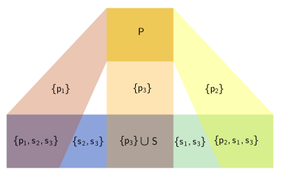
Figure 20: A good cover realization of $\mathcal{C}_{2}~{}=~{}\{\varnothing,23,13,4,5,6,234,135,1236,456\}.$ Here $P=\{1,2,3\}$ and $S=\{4,5,6\}$.

The proof of Theorem 0.2 depends on some basic facts about tope graphs of oriented matroids. The tope graph $\mathcal{T}$ of an oriented matroid $\mathcal{M}$ is a graph whose vertices are the topes of $\mathcal{M}$, and whose edges connect pairs of topes which differ by one sign. A subgraph $\mathcal{Q}\subseteq\mathcal{T}$ is called $T$-convex if it contains the shortest path between any two of its members. Any $e\in E$ divides the tope graph into two half-spaces $\mathcal{T}_{e}^{+}=\{W\in\mathcal{W}\mid e\in W^{+}\}$ and $\mathcal{T}_{e}^{-}=\{W\in\mathcal{W}\mid e\in W^{-}\}$. A subgraph $\mathcal{Q}\subseteq\mathcal{T}$ is $T$-convex if and only if it is an intersection of half-spaces [40, Proposition 4.2.6].

Theorem 0.2.

For each $n\geq 2$, the code $\mathcal{C}_{n}\not\leq\mathsf{L}^{+}(\mathcal{M})$ for any oriented matroid $\mathcal{M}$.

Proof.

Fix $n\geq 2$. Suppose to the contrary that there is an oriented matroid $\mathcal{M}$ such that $\mathcal{C}_{n}\leq\mathsf{L}^{+}(\mathcal{M})$. For ease of notation, let $\mathcal{M}$ denote the code $\mathsf{L}^{+}(\mathcal{M})$. Since $\varnothing\in\mathcal{C}_{n}$, we can assume without loss of generality that $\mathcal{C}_{n}=f(\mathcal{M})$ for some code morphism $f$.

Denote the ground set of $\mathcal{M}$ by $E$. The map $f$ must be defined by trunks

$$\operatorname{trunk}_{\mathcal{M}}(\pi_{1}),\dots,\operatorname{trunk}_{\mathcal{M}}(\pi_{n+1}),\operatorname{trunk}_{\mathcal{M}}(\sigma_{1}),\ldots,\operatorname{trunk}_{\mathcal{M}}(\sigma_{n+1}),$$

with $\pi_{i},\sigma_{i}\subseteq E$ corresponding to $p_{i}$ and $s_{i}$ respectively.

Claim 1: There is a tope $T$ of $\mathcal{M}$ such that $\left(\bigcup_{i=1}^{n+1}\sigma_{i}\right)\cup\left(\bigcap_{j=1}^{n}\pi_{j}\right)\cup\pi_{n+1}\subseteq T^{+}$.
Roughly speaking, we are producing a codeword in the intersection of the last petal and all simplices, which also lies in the convex hull of the other petals.

Define a morphism $g:\mathcal{M}\to 2^{[n+1]}$ by the trunks $T_{i}=\operatorname{trunk}_{\mathcal{M}}(\tau_{i})$, with $\tau_{i}=\sigma_{i}\cup\left(\,\,\bigcap_{j=1}^{n}{\pi_{j}}\,\right)$ for $i=1,\ldots,n+1$. Let $\mathcal{D}=g(\mathcal{M})$.

Since $(S\setminus\{s_{i}\})\cup\{p_{i}\}\in\mathcal{C}_{n}$ for each $i\in[n]$, we deduce that $[n+1]\setminus i$ is a codeword of $\mathcal{D}$ for each $i\in[n]$. Thus, $\operatorname{link}_{\{n+1\}}(\Delta(\mathcal{D}))$ is either a hollow $(n-1)$-simplex or a solid $(n-1)$- simplex. Since we have defined $\mathcal{D}$ as the image of an oriented matroid code, it cannot have local obstructions. The codeword $\{n+1\}$ is not in $\mathcal{D}$; if it were, then $f(g^{-1}(\{n+1\}))$ would be a codeword of $\mathcal{C}$ including $s_{n+1}$ without any other $s_{i}$. No such codeword exists in $\mathcal{C}$. Thus $\operatorname{link}_{\{n+1\}}(\Delta(\mathcal{D}))$ must be contractible. Because $\{n+1\}$ is not a codeword of $\mathcal{D}$, the $\operatorname{link}_{\{n+1\}}(\Delta(\mathcal{D}))$ must be a solid $(n-1)$-simplex; therefore, $[n+1]$ is a codeword of $\mathcal{D}$.

Based on the trunks defining $g$, we know that $\left(\bigcup_{i=1}^{n+1}\sigma_{i}\right)\cup\left(\bigcap_{j=1}^{n}\pi_{j}\right)\subseteq g^{-1}([n+1])$. By definition of $f$, we must also have $S\subseteq f(g^{-1}([n+1]))$; however, the only codeword of $\mathcal{C}_{n}$ which contains $S$ is $S\cup\{p_{n+1}\}$. Thus, there is a codeword of $\mathcal{M}$ containing $\left(\bigcup_{i=1}^{n+1}\sigma_{i}\right)\cup\left(\bigcap_{j=1}^{n}\pi_{j}\right)\cup\pi_{n+1}$. This implies that $\mathcal{M}$ has a covector $X$ such that $\left(\bigcup_{i=1}^{n+1}\sigma_{i}\right)\cup\left(\bigcap_{j=1}^{n}\pi_{j}\right)\cup\pi_{n+1}\subseteq X^{+}$. To produce a tope satisfying the condition, take $T=X\circ W$ for any tope $W$ of $\mathcal{M}$.

Claim 2: $\pi_{n+1}\cup\left(\,\,\bigcap_{j=1}^{n}\,\pi_{j}\right)\subseteq T^{+}$ implies $\,\,\bigcup_{j=1}^{n+1}\,\pi_{j}\subseteq T^{+}$ for any tope $T$ of $\mathcal{M}$.
The intuition here is that the last petal must intersect the convex hull of the other petals only in the common intersection of all petals, as illustrated in Figure 21.

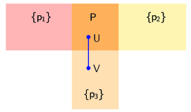
Figure 21: Any path from a tope $U$ with $\left(\bigcup_{j=1}^{n+1}\,\pi_{j}\right)\subseteq U^{+}$ to a tope $V$ with $\left(\bigcup_{j=1}^{n+1}\,\pi_{j}\right)\not\subseteq V^{+}$ must cross an edge in $\left(\bigcap_{j=1}^{n+1}\,\pi_{j}\right)$. Analogously, a path from a point in the atom $P=\{p_{1},p_{2},\ldots,p_{n+1}\}$ to the atom $\{p_{n+1}\}$ must cross the boundaries of $p_{1},p_{2},\ldots,p_{n}$ all at one time.

Let $U$ be a tope with $\left(\bigcup_{j=1}^{n+1}\,\pi_{j}\right)\subseteq U^{+}$. Such a tope must exist, since $P\in\mathcal{C}_{n}$. Suppose for the sake of contradiction that there exists a tope $V$ such that

$$\pi_{n+1}\cup\left(\,\,\bigcap_{j=1}^{n+1}\,\pi_{j}\right)\subseteq V^{+},\text{ but }\bigcup_{j=1}^{n+1}\,\pi_{j}\not\subseteq V^{+}.$$

Consider a shortest path from $U$ to $V$ in the tope graph of $\mathcal{M}$. Each edge of the tope graph is naturally labeled by the ground set element $e$ by which the two incident topes differ. By the $T$-convexity of intersections of half-spaces in the tope graph, each tope along this path has $\pi_{n+1}\cup\left(\,\bigcap_{j=1}^{n}\,\pi_{j}\right)$ in its positive part, so no edge is labeled with an element of $\bigcap_{j=1}^{n}\,\pi_{j}$.

Thus at some point along the path from $U$ to $V$, we must cross an edge $(T,W)$ labeled by a ground set element $e\in\left(\,\,\bigcup_{j=1}^{n+1}\,\pi_{j}\right)\setminus\left(\,\,\bigcap_{j=1}^{n+1}\,\pi_{j}\right)$. Choose the first such edge $(T,W)$ labeled with ground set element $e$. By our choice of $e$, there exist $k,\ell\in[n]$ such that $e\in\pi_{k}$, and $e\notin\pi_{\ell}$. This means $\pi_{k}\not\subseteq W^{+}$, whereas $\pi_{\ell}\subseteq W^{+}$. Then $\{p_{\ell},p_{n+1}\}\subseteq f(W^{+})$, but $f(W^{+})\neq P$. However, the only codeword of $\mathcal{C}_{n}$ containing $\{p_{\ell},p_{n+1}\}$ is $P$, so we have reached a contradiction. Therefore, no such tope $V$ may exist.

By Claim 1, $\mathcal{M}$ must have a tope $T$ which has $\left(\bigcup_{i=1}^{n+1}\sigma_{i}\right)\cup\left(\bigcup_{j=1}^{n}\pi_{1}\right)\cup\pi_{n+1}\subseteq T^{+}$. Because $T$ satisfies $\left(\bigcap_{i=1}^{n+1}\pi_{i}\right)\cup\pi_{n+1}\subseteq T^{+}$, Claim 2 implies that $\bigcup_{i=1}^{n+1}\pi_{i}\subseteq T^{+}$. Therefore, $\left(\bigcup_{i=1}^{n+1}\pi_{i}\right)\cup\left(\bigcup_{i=1}^{n+1}\sigma_{i}\right)\subseteq T^{+}$, but this implies $f(T)=P\cup S\in\mathcal{C}_{n}$, a contradiction. ∎

By showing that the family of codes $\{\mathcal{C}_{n}\}_{n\geq 2}$ do not lie below oriented matroids, we have given an alternate proof that these codes do not have realizations with interiors of convex polytopes. This proof is significantly different in structure than the original proof that these codes are not convex using Theorem 0.6, which is in turn proved by induction on dimension. In contrast, our proof makes no reference to rank or dimension, and does not use induction. While the codes $\{\mathcal{C}_{n}\}_{n}$ are not open convex, they do have realizations with closed convex sets, which can even be chosen to be (non-full dimensional) closed convex polytopes. Notice that Theorem 0.1 establishes that if $\mathcal{C}$ has a realization with interiors of convex polytopes, then $\mathcal{C}\leq\mathsf{L}^{+}(\mathcal{M})$. However, the fact that a code has a realization with closed convex polytopes does not guarantee this. Further, in showing that these codes do not lie below any oriented matroids at all, we have established that, even while these codes are good cover codes, their obstructions to convexity are somehow still topological in nature.

Representability and convexity

Having exhibited that many well-known non-convex codes do not lie below any oriented matroids at all, we now exhibit a family of non-convex codes which lie below non-representable oriented matroids. For each uniform, rank 3 affine oriented matroid $(\mathcal{M},g)$, we construct a code $\mathcal{C}(\mathcal{M},g)$ which is convex if and only if $\mathcal{M}$ is representable (recall a uniform oriented matroid is one in which all circuits have the same cardinality). Moreover, this code is always the image of an oriented matroid under a code morphism.

Consider a uniform, affine oriented matroid $(\mathcal{M},g)$ of rank 3. A pseudoline is a simple unbounded curve $L$ in $\mathbb{R}^{2}$, which partitions the plane into pieces $\mathbb{R}^{2}=L^{+}\sqcup L\sqcup L^{-}$. By the topological representation theorem ([40, Section 1.3],[52]), $(\mathcal{M},g)$ can be represented by a uniform arrangement of piecewise linear pseudolines, that is, a family $\mathcal{P}=\{L_{i}\}_{i\in[n]}$ of pseudolines such that each pair intersects exactly once and no more than two meet at any point. The sign vectors of this arrangement are the covectors of $(\mathcal{M},g)$. An example is illustrated in 22.

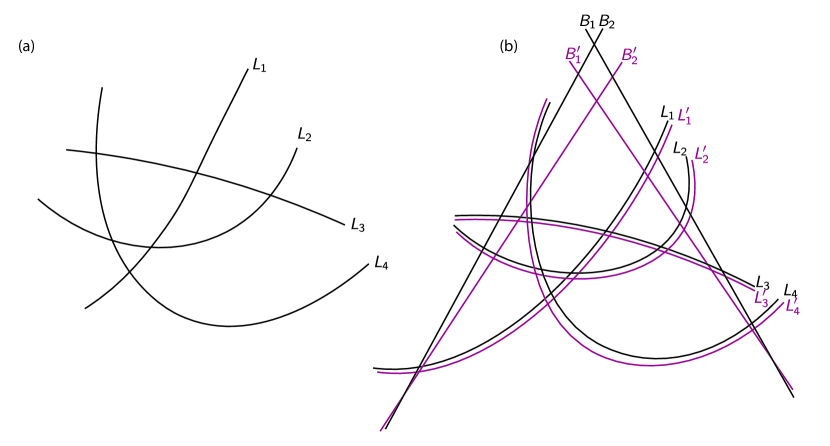
Figure 22: (a) An arrangement of four pseudolines corresponding to an affine oriented matroid $(\mathcal{M},g)$. (b) The augmented pseudoline arrangement $\mathcal{M}^{\prime}$ used in the proof of Proposition 0.6.

Note that the oriented matroid of a pseudoline arrangement is completely determined by the order in which each line meets all of the other lines. We can record this information as follows: Let $L_{1},\ldots,L_{n}$ be a pseudoline arrangement. For each pseudoline, fix one end of the pseudoline as the “head". Let $\pi_{i}(j)$ denote the index $k$ such that $L_{j}$ is the $k^{\mathrm{th}}$ pseudoline we encounter as we follow $L_{i}$ from the head to the tail.

We use this order to define a code $\mathcal{C}(\mathcal{M},g)$. We will then use the concept of order-forcing, introduced in the previous chapter, to prove that this code is convex if and only if $\mathcal{M}$ is representable.

Now, we construct the code $\mathcal{C}(\mathcal{M},g)$ so that a sequence of codewords along each pseudoline is order-forced.

Definition 0.24.

Let $(\mathcal{M},g)$ be a uniform, affine oriented matroid of rank 3 with pseudoline arrangement $L_{1},\ldots,L_{n}$. Relabel the pseudolines $L_{1},\ldots,L_{n}$, with their heads in clockwise order around the outside of the plane. An example is illustrated in Figure 22.

$\mathcal{C}(\mathcal{M},g)$ is a code on $n+2+n^{2}+2n=(n+1)(n+2)$ neurons, labeled:

$a_{1},\ldots,a_{n}$:	Strips corresponding to each pseudoline of $\mathcal{M}$.
$b_{\ell},b_{r}$:	Strips corresponding to two new “boundary” pseudolines whose positive quadrant includes all pseudoline intersections.
$c_{1,1},c_{1,2},\ldots,c_{n,n}$:	$n$ neurons along each $a_{i}$ to apply order-forcing.
$d_{\ell,1},d_{\ell,2},\ldots,d_{\ell,n},\ldots,d_{r,n}$:	$n$ neurons along $b_{r}$ and $b_{\ell}$ to apply order-forcing.

The codewords of $\mathcal{C}(\mathcal{M},g)$ are as follows:

$b_{\ell}b_{r}d_{\ell,1}d_{r,1}$:	Intersection of the two boundary strips.
$b_{s}d_{s,j}$:	Order-forcing along each boundary strip
	($s=\ell,r$, $j=1,\ldots,n$.)
$b_{r}a_{i}d_{r,i}d_{r,i+1}c_{i,1}$:	Intersection of each pseudoline with right boundary strip, with order-forcing neurons. ($i=1,\ldots,n-1$)
$b_{r}a_{n}d_{r,n}c_{n,1}$:	Intersection of final pseudoline with right boundary strip (one less order-forcing neuron is required.)
$b_{\ell}a_{n+1-i}d_{\ell,i}d_{\ell,i+1}c_{n+1-i,n}$:	Intersection of each pseudoline with left boundary strip plus order-forcing neurons. ($i=1,\ldots,n-1$.)
$b_{\ell}a_{1}d_{\ell,n}c_{1,n}$:	Intersection of first pseudoline with left boundary strip.
$a_{i}c_{ij}$:	Order-forcing along each pseudoline
	($i=1,\ldots,n$, $j=1,\ldots,n$)
$a_{i}a_{j}c_{i,\pi_{i}(j)}c_{i,\pi_{i}(j)+1}$	Pairwise intersections of pseudolines plus order-forcing
$c_{j,\pi_{j}(i)}c_{j,\pi_{j}(i)+1}$:	($i=1,\ldots,n$, $j=1,\ldots,n-1$.)

We include an example of a good cover realization of this code in Figure 23. Note that this code resembles the code $\mathcal{R}$ from the previous chapter.

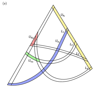
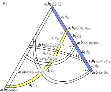
Figure 23: A good-cover realization of the code $\mathcal{C}(\mathcal{M},g)$ for the oriented matroid of the pseudoline arrangement $L_{1},L_{2},L_{3},L_{4}$. (a) The sets $U_{x}$ corresponding to neurons $x$ of $\mathcal{C}(\mathcal{M},g)$. (b) The codewords of $\mathcal{C}(\mathcal{M},g)$. For clarity, only the codewords arising from $U_{a_{1}}$ and $U_{b_{r}}$ are labeled.

Proposition 0.6.

For any uniform, rank 3 affine oriented matroid $(\mathcal{M},g)$, there exists a rank 3 oriented matroid $\widehat{\mathcal{M}}$ such that $\mathcal{C}(\mathcal{M},g)\leq\mathsf{L}^{+}\widehat{\mathcal{M}}$.

Proof.

We describe the pseudoline arrangement associated to $\widehat{\mathcal{M}}$. Fix a piecewise-linear pseudoline arrangement $L_{1},\ldots,L_{n}$ representing $(\mathcal{M},g)$ consistent with the labeling in $\mathcal{C}(\mathcal{M},g)$. Let $B_{r}$ be a line which meets $L_{1},L_{2},\ldots,L_{n}$ in the clockwise order consistent with the labeling. Let $B_{\ell}$ be a line which meets $B_{r}$ and then $L_{n},L_{n-1},\ldots,L_{1}$ in the opposite of this clockwise order. Orient $B_{r}$ and $B_{\ell}$ such that $B_{r}^{+}$ and $B_{\ell}^{+}$ are the half-spaces containing all bounded cells of the pseudoline arrangement. Orient each $L_{i}$ such that $B_{r}\cap B_{\ell}$ lies in $L_{i}^{-}$.

Now, for each $i\in[n]$, we define a pseudoline $L^{\prime}$ which acts as a translation of $L_{i}$ into its positive half-space. That is, we let $L_{i}^{\prime}$ be a pseudoline which intersects $B_{\ell},B_{r}$ each $L_{j},j\neq i$ in the same order as $L_{i}$, and such that for each other pseudoline $L$, the intersections of $L_{i}$ and $L_{i}^{\prime}$ are adjacent along $L$. Further, we ensure that $L_{i},L_{i}^{\prime}$ do not intersect. Orient $L_{i}^{\prime}$ so that $L_{i}\subseteq L_{i}^{\prime+}$. Define $B_{\ell}^{\prime},B_{r}^{\prime}$ and orient them analogously.

Finally, we produce an oriented matroid $\widehat{\mathcal{M}}$ from this pseudoline arrangement by fixing a ground set element $h$ such that the set of covectors of the pseudoline arrangement is the affine space of $(\widehat{\mathcal{M}},h)$. We claim the oriented matroid of this arrangement, $\widehat{\mathcal{M}}$, lies above $\mathcal{C}(\mathcal{M},g)$. The morphism $f$ such that $f(\operatorname{trunk}_{\mathsf{L}^{+}\widehat{\mathcal{M}}}(h))=\mathcal{C}(\mathcal{M},g)$ is defined by the the trunks

$$\{T_{a_{i}}\}_{i=1,\ldots,n}\cup\{T_{b_{r}},T_{b_{\ell}}\}\cup\{T_{c_{i,j}}\}_{i=1,\ldots,n,j=1,\ldots,n}\cup\{T_{d_{s,j}}\}_{s=r,\ell,j=1,\ldots,n}.$$

corresponding to the neurons of $\mathcal{C}(\mathcal{M},g)$. These trunks are defined as follows:

$$T_{a_{i}} :=\{i,i^{\prime},r,\ell\}\mbox{ for }i=1,\ldots,n$$

$$T_{b_{r}} :=\{r,r^{\prime},\ell,n^{\prime}\}$$

$$T_{b_{\ell}} :=\{\ell,\ell^{\prime},r,n^{\prime}\}$$

$$T_{d_{r,1}} :=\{r,r^{\prime},\ell,1^{\prime}\}$$

$$T_{d_{r,i}} :=\{r,r^{\prime},{i-1},{i}^{\prime}\}\mbox{ for }i=2,\ldots,n$$

$$T_{d_{\ell,1}} :=\{\ell,\ell^{\prime},r,n^{\prime}\}$$

$$T_{d_{\ell,i}} :=\{\ell,\ell^{\prime},{n-i+2},{n-i+1}^{\prime}\}\mbox{ for }i=2,\ldots,n.$$

In order to define $T_{c_{i,j}}$, we introduce some notation. Let

$$L_{1}(i,j)=\begin{cases}j\mbox{ if }j<i\\ j^{\prime}\mbox{ if }j>i\end{cases}\qquad L_{2}(i,j)=\begin{cases}j^{\prime}\mbox{ if }j<i\\ j\mbox{ if }j>i\\ \end{cases}.$$

That is, $L_{1}(i,j)$ is whichever of $j,j^{\prime}$ the line $L_{1}$ meets first as we follow it from its intersection with $B_{r}$ to its intersection with $B_{\ell}$, and $L_{2}(i,j)$ is whichever it hits second. Now, we define

$$T_{c_{i1}} :=\{i,i^{\prime},r,L_{2}(i,\pi(i,1))\}\mbox{ for }i=1,\ldots,n$$

$$T_{c_{ij}} :=\{i,i^{\prime},L_{1}(i,\pi(i,j-1)),L_{2}(i,\pi(i,j-1))\}\mbox{ for }i=1,\ldots,n,j=2,\ldots,n-1$$

$$T_{c_{in}} :=\{i,i^{\prime},L_{1}(i,\pi(i,n-1)),\ell\}\mbox{ for }i=1,\ldots,n,j=2,\ldots,n-1.$$

Finally, we verify that the map $f(\sigma)=\{s\mid\sigma\in T_{s}\}$ has image $\mathcal{C}(\mathcal{M},g)$. This follows from the fact that the good cover arising from $\{B_{s}^{+}\cap B_{s}^{\prime+}\}_{s=\ell,r}\cup\{L_{i}^{+}\cap L_{i}^{\prime+}\}_{i=1,\ldots,n}$ gives rise to a good cover realization of $\mathcal{C}(\mathcal{M},g)$. This completes the proof. ∎

Theorem 0.3.

Let $\mathcal{M}=(E,\mathcal{L})$ be a uniform, rank 3 oriented matroid. Then for $g\in E$, the code $\mathcal{C}(\mathcal{M},g)$ is convex if and only if $\mathcal{M}$ is representable.

Proof.

First, we show that if $\mathcal{M}$ is representable, $\mathcal{C}(\mathcal{M},g)$ is convex. Note that by Proposition 0.6, we have that $\mathcal{C}(\mathcal{M},g)\leq\mathsf{L}^{+}\widehat{\mathcal{M}}$. Also note that by construction, if $\mathcal{M}$ is representable, then so is $\widehat{\mathcal{M}}$. Therefore, by Theorem 0.1, if $\mathcal{M}$ is representable, $\mathcal{C}(\mathcal{M},g)$ is convex.

Next, we show that if $\mathcal{C}(\mathcal{M},g)$ is convex, then $\mathcal{M}$ is representable. Note that the following sequences are order-forced in $\mathcal{C}(\mathcal{M},g)$.

1. The only feasible path from $b_{r}b_{\ell}d_{r1}d_{\ell 1}$ to $b_{r}a_{n}d_{rn}$ in $G_{\mathcal{C}(\mathcal{M},g)}$ is

   $$b_{r}b_{\ell}d_{r1}d_{\ell 1}\leftrightarrow b_{r}d_{r1}\leftrightarrow b_{r}a_{1}d_{r1}d_{r2}\leftrightarrow b_{r}d_{r2}\leftrightarrow\cdots\leftrightarrow b_{r}d_{rn}\leftrightarrow b_{r}a_{n}d_{rn}$$

2. The only feasible path from $b_{r}b_{\ell}d_{r1}d_{\ell 1}$ to $b_{\ell}a_{1}d_{\ell n}$ in $G_{\mathcal{C}(\mathcal{M},g)}$ is

   $$b_{r}b_{\ell}d_{r1}d_{\ell 1}\leftrightarrow b_{\ell}d_{\ell 1}\leftrightarrow b_{\ell}a_{n}d_{\ell 1}d_{\ell 2}\leftrightarrow b_{r}d_{\ell 2}\leftrightarrow\cdots\leftrightarrow b_{\ell}d_{\ell n}\leftrightarrow b_{\ell}a_{1}d_{\ell n}$$

3. For each $i$, the only feasible path from $b_{r}a_{i}c_{i1}d_{ri}d_{ri+1}$ to $a_{i}b_{\ell}c_{in}d_{\ell(n-i+1)}$ in
   $G_{\mathcal{C}(\mathcal{M},g)}$ is

   $$b_{r}a_{i}c_{i1}d_{ri}d_{ri+1} \leftrightarrow a_{i}c_{i1}\leftrightarrow a_{i}a_{\pi^{-1}_{i}(1)}c_{i1}c_{i2}c_{\pi^{-1}_{i}(1),\pi_{\pi^{-1}_{i}(1)}(i)}c_{\pi^{-1}_{i}(1),\pi_{\pi^{-1}_{i}(1)}(i)+1}$$

   $$\cdots \leftrightarrow a_{i}c_{i2}\leftrightarrow a_{i}c_{i(n-1)}$$

   $$\cdots \leftrightarrow a_{i}a_{\pi^{-1}_{i}(n-1)}c_{i(n-1)}c_{in}c_{\pi^{-1}_{i}((n-1)),\pi_{\pi^{-1}_{i}(n-1)}(i)}c_{\pi^{-1}_{i}(1),\pi_{\pi^{-1}_{i}(n-1)}(i)+1}$$

   $$\cdots \leftrightarrow a_{i}c_{in}\leftrightarrow a_{i}b_{\ell}c_{in}d_{\ell(n-i+1)}$$

We claim if $\mathcal{C}(\mathcal{M},g)$ is convex, then it has a realization in the plane. Suppose that $\mathcal{C}(\mathcal{M},g)$ is convex, and fix a realization $\mathcal{U}$ in $\mathbb{R}^{d}$. Choose points $p_{1},p_{2},p_{3}$ in the atoms $A_{b_{r}b_{\ell}d_{r1}d_{\ell 1}}$, $A_{b_{r}a_{n}d_{rn}}$, and $A_{b_{\ell}a_{1}d_{\ell n}}$ respectively. We will show that each atom in this realization has a nonempty intersection with $\operatorname{conv}(p_{1},p_{2},p_{3})$. By order forcing (1), the line from $p_{1}$ to $p_{2}$ must pass through the atoms of all codewords containing $b_{r}$ in the listed order. Likewise, by order forcing (2), the line from $p_{1}$ to $p_{3}$ must pass through the atoms of all codewords containing $b_{\ell}$ in the listed order.

In particular, we have shown that for each $i$, the atoms of $\sigma=b_{r}a_{i}d_{ri}d_{r(i+1)}c_{i1}$ and $\tau=b_{\ell}a_{i}d_{\ell(n+1-i)}d_{\ell(n+2-i)}c_{i1}$ have a nonempty intersection with $\operatorname{conv}(p_{1},p_{2},p_{3})$. For each $i$, pick a point $q_{i}\in\operatorname{conv}(p_{1},p_{2},p_{3})\cap A_{\sigma}$ and a point $r_{i}\in\operatorname{conv}(p_{1},p_{2},p_{3})\cap A_{\tau}$. Applying order forcing (3) for each $i$, we have that the line from $r_{i}$ to $q_{i}$ passes through the atoms of all codewords containing $a_{i}$, in the listed order. This accounts for every codeword of $\mathcal{C}(\mathcal{M},g)$. Thus, intersecting the open sets in $\mathcal{U}$ with the plane $\mathrm{aff}(p_{1},p_{2},p_{3})$ produces a two-dimensional convex realization of $\mathcal{C}(\mathcal{M},g)$.

Now, we obtain a straight line arrangement for $(\mathcal{M},g)$ in this plane by extending the line segment from $q_{i}$ to $r_{i}$ to be a line. Notice that by order forcing (3), this line meets the sets $U_{a_{1}},\ldots,U_{a_{n}}$ in the order consistent with the pseudoline arrangement. Thus, if this code is convex, then the pseudoline arrangement is stretchable, and thus $\mathcal{M}$ is representable. ∎

Proposition 0.3 demonstrates that matroid representability and convex code realizability are intertwined. One consequence is that non-representable oriented matroids are a new source for constructing non-realizable codes:

Corollary 0.3.

There is an infinite family of non-convex codes which lie below oriented matroids in $P_{\operatorname{code}}$.

Proof.

There are infinitely many non-representable uniform oriented matroids of rank 3 [40, Proposition 8.3.1]. By Proposition 0.3, $\mathcal{C}(\mathcal{M},g)$ is non-convex for each of these. By Proposition 0.6, $\mathcal{C}(\mathcal{M},g)\leq\mathsf{L}^{+}\widehat{\mathcal{M}}$. ∎

Example 0.6.

Let $(\mathcal{M},g)$ be the uniform non-Pappus matroid from [26], whose pseudoline arrangement appears in Figure 24. This matroid is non-representable, since a realization of it would violate Pappus’s hexagon thoerem. Then $\mathcal{C}(\mathcal{M},g)$ is a non-convex code with no local obstructions.

Figure 24: The pseudoline arrangement for the uniform non-Pappus matroid.

The convex code decision problem is NP-hard

We now turn to the computational aspects of convex codes. Using the relationship between convex codes and representable oriented matroids (Theorem 0.3), we demonstrate the convex code decision problem is NP-hard and $\exists\mathbb{R}$-hard, though it remains open whether the convex code decision problem lies in either of these classes, or is even decidable. The complexity class $\exists\mathbb{R}$, read as the existential theory of the reals, is the class of decision problems of the form

$$\exists(x_{1}\in\mathbb{R})\ldots\exists(x_{n}\in\mathbb{R})P(x_{1},\ldots,x_{n}),$$

where $P$ is a quantifier-free formula whose atomic formulas are polynomial equations, inequations, and inequalities in the $x_{i}$. In other words, a problem in $\exists\mathbb{R}$ defines a semialgebraic set over the real numbers and asks whether or not it contains any points [broglia2011lectures]. Many well known problems in computational geometry lie in $\exists\mathbb{R}$, including some problems very similar to determining whether a code is convex. For instance, determining whether a graph is the intersection graph of convex sets in the plane is $\exists\mathbb{R}$ complete [54].

Theorem 0.3 implies the convex code decision problem is at least as difficult as deciding if an oriented matroid is representable. This decision problem is $\exists\mathbb{R}$-complete [25, 26, 24] and therefore the convex code decision problem is $\exists\mathbb{R}$-hard.

Theorem 0.4.

Any problem in $\exists\mathbb{R}$ can be reduced in polynomial time to the problem of determining whether a neural code is convex.

Proof.

By the Mnëv-Sturmfels universality theorem (see [25, 24, 26, 40]), determining whether a rank 3 uniform oriented matroid is representable is complete for the existential theory of the reals. By Proposition 0.3, a rank 3 uniform oriented matroid $\mathcal{M}$ is representable if and only if $\mathcal{C}(\mathcal{M},g)$ is a convex neural code. Further, the number of neurons in $\mathcal{C}(\mathcal{M},g)$ is quadratic in the size of the ground set of $\mathcal{M}$, and the number of codewords of $\mathcal{C}(\mathcal{M},g)$ is less than the number of covectors of $\mathcal{M}$. Any problem in $\exists\mathbb{R}$ can be reduced in polynomial time to deciding representability of a uniform oriented matroid and thus convexity of the corresponding code. ∎

Since any $\exists\mathbb{R}$ complete problem is also $\mathrm{NP}$-hard, we have as a corollary that determining whether a code is convex is $\mathrm{NP}$-hard.

Corollary 0.4.

The problem of determining whether a code is convex is $\mathrm{NP}$-hard, where the problem size is measured in the number of codewords.

Notice that because we can perform this reduction of a problem in $\exists\mathbb{R}$ to a neural code in polynomial time, this result holds even when we measure the problem size in terms of the number of codewords, which may be exponentially large in the number of neurons. Again, this NP hardness result is not surprising. For instance, it parallels the result that recognizing whether a simplicial complex is the nerve of convex sets in $\mathbb{R}^{d}$ is $\mathrm{NP}$-hard for $d\geq 2$ [49].

Open questions

The preceding sections have presented our case for employing oriented matroid theory in the study of neural codes. However, we stand at the very beginning of exploring this connection. In this section, we outline some directions for future work.

Concrete Examples

Question 0.7.

Are the non convex codes $\mathcal{T}$ and $\mathcal{R}$ from the previous chapter images of oriented matroids?

Is the missing axiom of convex codes also lost forever?

While general neural codes are not required to satisfy any axioms, the codes below oriented matroids may be more tractable to combinatorial description.

Question 0.8.

Can the class of neural codes below oriented matroids be characterized by a set of combinatorial axioms?

If this question is answered in the affirmative, then these codes can be thought of as “partial oriented matroids.” Suppose that $\mathcal{C}\subseteq 2^{[n]}$ is a code and $\mathcal{M}$ is an oriented matroid on ground set $[N]$ such that $\mathcal{C}=f(\mathsf{L}^{+}(\mathcal{M}))$; then, we obtain constraints on the set of covectors of $\mathcal{M}$. Each included codeword $\sigma\in\mathcal{C}$ implies existence of a preimage covector in $\mathcal{M}$, and each excluded codeword $\tau\notin\mathcal{C}$ implies a set of forbidden covectors which may not be in $\mathcal{M}$. The oriented matroids satisfying these constraints can then be said to be “completions” of the partial oriented matroid.

Just as we wish to characterize codes lying below oriented matroids with a set of combinatorial axioms, we might also wish to characterize convex codes using a set of combinatorial axioms. However, this is likely not possible. In [57], Mayhew, Newman, and Whittle show that “the missing axiom of matroid theory is lost forever." Slightly more formally, they show that there is no sentence characterizing representability in the monadic second order language $MS_{0}$, which is strong enough to state the standard matroid axioms. Roughly, this means that there is no “combinatorial" characterization of representability, or no characterization of representability in the language of the other matroid axioms.

Because we have found strong connections between representability and convexity, it is natural to ask whether a similar statement can be proven for convex codes.

Question 0.9.

Is there a natural language in which we can state “combinatorial" properties of neural codes, in analogy with the $MS_{0}$ for matroids? If so, is it possible to characterize convexity in this language?

Computational questions

While we have shown that the convex code decision problem is $\exists\mathbb{R}$-hard, we have not actually shown that the convex code decision problem lies in $\exists\mathbb{R}$, or is even algorithmically decidable. A similar problem, that of determining whether a code has a good cover realization, is undecidable by [7, Theorem 4.5]. Here, the distinction between codes with good cover realizations and convex realizations may be significant. For instance, while there is an algorithm to decide whether, for any given $d$, a simplicial complex is the nerve of convex open subsets of $\mathbb{R}^{d}$, for each $d\geq 5$, it is algorithmically undecidable whether a simplicial complex is the nerve of a good cover in $\mathbb{R}^{d}$ [66].

We outline a possible path towards resolving [7, Question 4.5], which asks whether there is an algorithm which decides whether a code is convex. Our approach hinges on 0.1: a code is polytope convex if and only if it lies below a representable oriented matroid. A first step towards solving the convex code decision problem is answering the following open question:

Question 0.10.

Can every convex code be realized with convex polytopes?

If this can be answered in the affirmative, then our Theorem 0.1 becomes strengthened to the following:

Conjecture 0.1.

A code $\mathcal{C}$ is convex if and only if $\mathcal{C}\leq\sf{L}^{+}\mathcal{M}$ for $\mathcal{M}$ a representable oriented matroid.

If this conjecture holds, then we can replace the problem of determining whether a code is convex with the problem of determining whether a code lies below a representable matroid. We only need to enumerate matroids above the code, and then check these matroids for representability.

Question 0.11.

Given a code $\mathcal{C}$, is there an algorithm to enumerate the set of oriented matroids $\mathcal{M}$ which lie above $\mathcal{C}$?

One way to find oriented matroids above a code $\mathcal{C}$ is to travel step-by-step up the poset $P_{\operatorname{code}}$. While there is a straightforward algorithm to enumerate the $O(n)$ codes which are covered by a code $\mathcal{C}\subseteq 2^{[n]}$ in $\mathbf{P}_{\mathbf{Code}}$ [9], we do not know of a straightforward way to characterize the codes which cover $\mathcal{C}$. If we can characterize these codes as well, we may be able to find a way to “climb up” towards an oriented matroid. Alternatively, we can use the “partial oriented matroid” perspective described above to obtain a set of constraints that must be obeyed by any oriented matroid above this code. Then we can look for a matroid satisfying these constraints.

Both of these approaches depend on the minimal size of the ground set of oriented matroids that lie above $\mathcal{C}$ in $P_{\operatorname{code}}$. Let

$$M(n)=\max_{\begin{subarray}{c}\mathcal{C}\subseteq 2^{[n]}\\ \mathcal{C}\mbox{ \scriptsize below an}\\ \mbox{ \scriptsize oriented matroid}\end{subarray}}\left[\min_{\mathcal{C}\leq\sf{L}^{+}(\mathcal{M})}|E(\mathcal{M})|\right]$$

be the smallest $N$ such that any code $\mathcal{C}$ on $n$ neurons which lies below an oriented matroid lies below an oriented matroid with ground set of size at most $N$. Similarly, let

$$H(n)=\max_{\begin{subarray}{c}\mathcal{C}\subseteq 2^{[n]}\\ \mathcal{C}\mbox{ \scriptsize below a representable}\\ \mbox{ \scriptsize oriented matroid}\end{subarray}}\left[\min_{\begin{subarray}{c}\mathcal{C}\leq\sf{L}^{+}\mathcal{M}\\ \mathcal{M}\mbox{ \scriptsize representable}\end{subarray}}|E(\mathcal{M})|\right]$$

be the smallest $N$ such that any code $\mathcal{C}$ on $n$ neurons below a representable oriented matroid lies below a representable oriented matroid with ground set of size at most $N$. Clearly, $M(n)\leq H(n)$, since any representable matroid is a matroid.

Question 0.12.

Describe the growth of $M(n)$ and $H(n)$ as functions of $n$. Are they equal?

Note that if $H(n)$ is a computable function of $n$, and Question 0.10 is answered in the affirmative, then the convex code decision problem is decidable.

Polyhedral approximation questions

The first part of this program is to prove Conjecture  0.10. Standard theorems about approximating convex bodies with convex polytopes suffice to prove that any simplicial complex is the nerve of a collection of interiors of convex polytopes. However, the code of a cover is a more delicate object than the nerve, so approximation techniques may fail.

Other questions in geometric combinatorics

Many classic theorems about convex sets, such as Helly’s theorem, Radon’s theorem, and Caratheodory’s theorem, have oriented matroid analogues. In some way, we can view our Theorem 0.2 as an oriented matroid version of Jeffs’ sunflower theorem [9, Theorem 1.1]. The fact that the non-convex codes constructed from the sunflower theorem do not lie below oriented matroids shows us that there is some fact about oriented matroids underlying the sunflower theorem.

Question 0.13.

Is there a natural oriented matroid version of Jeffs’ sunflower theorem?

Proposition 0.5 stated that if $\mathcal{M}$ is an oriented matroid, the code $\sf{L}^{+}\mathcal{M}$ has no local obstructions. That is, for any $\sigma\in\Delta(\sf{L}^{+}\mathcal{M})\setminus\sf{L}^{+}\mathcal{M}$, $\operatorname{link}_{\sigma}(\Delta(\sf{L}^{+}\mathcal{M}))$ is contractible. This result can also be found in [65], where is is phrased as a result about the simplicial complex $\Delta_{\mathrm{acyclic}}(\mathcal{M})$. Something stronger holds for representable oriented matroids: by [7, Theorem 5.10], if $\mathcal{M}$ is a representable oriented matroid, and $\sigma\in\Delta(\sf{L}^{+}\mathcal{M})\setminus\sf{L}^{+}\mathcal{M}$, then $\operatorname{link}_{\sigma}(\sf{L}^{+}\mathcal{M})$ must be collapsible. Expanding upon this work, [17] gives stronger conditions that the link of a missing codeword in a convex code must satisfy.

We ask whether this holds for all oriented matroids:

Question 0.14.

If $\mathcal{M}$ is an oriented matroid, and $\sigma\in\Delta(\sf{L}^{+}\mathcal{M})\setminus\sf{L}^{+}\mathcal{M}$, is $\operatorname{link}_{\sigma}(\Delta(\sf{L}^{+}\mathcal{M}))$ collapsible? More generally, which simplicial complexes can arise as $\operatorname{link}_{\sigma}(\Delta(\sf{L}^{+}\mathcal{M}))$ for $\sigma\in\Delta(\sf{L}^{+}\mathcal{M})\setminus\sf{L}^{+}\mathcal{M}$?

If not, then the non-collapsibility of $\operatorname{link}_{\sigma}(\Delta(\mathsf{L}^{+}(\mathcal{M})))$ gives a new “signature" of non-representability.

Underlying Rank

A Novel Notion of Rank for Neural Data Analysis

This chapter is adapted from an upcoming paper, which is joint work with Carina Curto, Juliana Londono Alvarez, and Hannah Rocio Santa Cruz [67].

Introduction

Monotone nonlinear transformations present challenges for data analysis in neuroscience and beyond. For instance, calcium imaging is a widely used tool for recording the activity of large populations of neurons. However, calcium fluorescence has a nonlinear, but monotone, relationship with underlying spiking activity [35, 68, 69]. This has consequences for analysis of population codes [36]. The nonlinear relationship between membrane potential and spiking activity also effects analysis of neural coding [70]. In psychology, signed difference analysis is used to evaluate models when there is an unknown monotone relationship between underlying psychological constructs and measured variables, such as task performance [71, 72]. In studies of gene interaction, there is often a monotone, nonlinear relationship between the trait genes directly act on and the trait we are are able to measure [73, 74, 75].

Here, we focus on estimating the dimensionality of neural activity in the presence of monotone nonlinear transformations. The dimensionality of neural activity has emerged as a key variable describing how populations of neurons encode stimuli and perform tasks [76, 77]. In many cases, neural activity has been observed to have dimensionality much lower than the number of neurons [78, 79, 80]. Standard linear methods for computing the dimensionality of neural activity rely on singular values, which are not stable under monotone nonlinear transformation. In Figure 25, we see the effect of the saturating monotone nonlinear transformation $f(x)=1-e^{-5x}$ on the singular vales of a $20\times 20$ matrix with rank 5. There is a sharp drop after the first five singular values, consistent with the low rank of the matrix. This drop does not appear in the transformed data: instead, singular values decay smoothly. How can we get around this to recover the original rank?

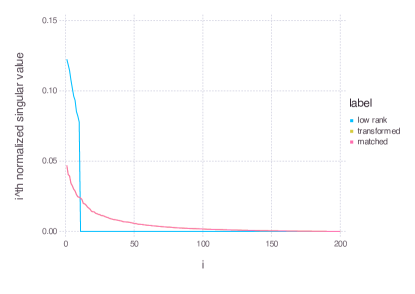
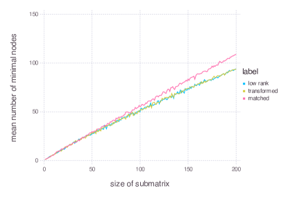
Figure 25: Left: We plot the normalized singular values for three $20\times 20$ matrices. The “low rank" matrix a random matrix with rank 5. The “transformed" matrix is the result of applying the saturating function $f(x)=1-e^{-5x}$ entrywise on the low rank matrix. Finally, the “matched" matrix is a random matrix generated to have the same singular values as the transformed matrix. The “transformed" and “matched" curve are indistinguishable, by construction. Right: We are able to distinguish the “transformed" and “matched" matrices using the technique of counting minimal nodes, introduced in Section Minimal nodes: a practical tool to estimate underlying rank of this paper. Because minimal modes are stable under monotone nonlinear transformations, the minimal node curves of the low-rank and transformed matrices overlap.

In this paper, we introduce the underlying rank of a matrix, a notion of rank which is stable under monotone nonlinear transformations. The underlying rank of a matrix $A$ is the minimal rank $d$ such that there exists a rank $d$ matrix $B$ and a monotone function $f$ such that $A_{ij}=f(B_{ij})$. In other words, the underlying rank of a matrix is the minimal rank consistent with the ordering of matrix entries. When we interpret the matrix $A$ as our data and our matrix $B$ as the unobserved underlying values, the underlying rank $d$ is a lower bound for the true dimensionality of our data. Our goal in this paper is to put the concept of underlying rank into mathematical context and to present techniques for estimating the underlying rank of a given matrix.

In Section The geometry of underlying rank, we show that we can associate a rank $d$ matrix to a pair of point configurations in $\mathbb{R}^{d}$. We show that it is possible to recover features of these point arrangements from the ordering of matrix entries. This makes it possible to bring toolset of discrete geometry in to estimate underlying rank. In Section Minimal nodes: a practical tool to estimate underlying rank, we introduce the minimal nodes of a matrix as a tool for estimating the underlying rank of a random matrix. In In Section Radon’s theorem: a lower bound for underlying rank, we apply Radon’s theorem to obtain lower bounds for underlying rank. Section Application: dimensionality of neural activity in the larval zebrafish optic tectum, we give a proof of concept by applying this analysis to calcium imaging data from the optic tectum in zebrafish larvae. Our discussion of underlying rank will continue into the next chapter, where we will relate underlying rank to oriented matroid theory and show that computing underlying rank is hard.

The geometry of underlying rank

We can decompose a rank $d$ matrix $A$ as a pair of point arrangements in $\mathbb{R}^{d}$. The order of entries of $A$ carries information about these point arrangements which can help us estimate the underlying rank of $A$.

In this section, we introduce the key idea of this paper, that which underlies all of our results: rank $d$ matrices correspond to point arrangements in $\mathbb{R}^{d}$ (Figure 26), and the ordering of matrix entries encodes geometric information about this point arrangement (Figure 27).

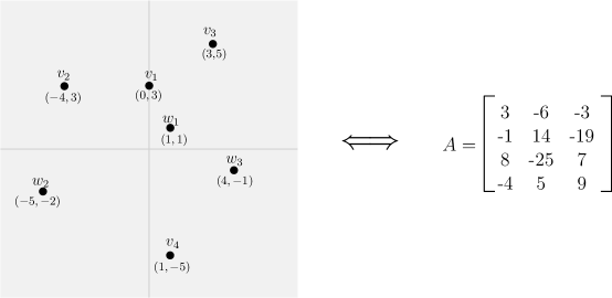
Figure 26: A point arrangement in $\mathbb{R}^{2}$ generating the matrix $A$.

Proposition 0.7.

Let $A$ be a $m\times n$ matrix of rank $d$ with real entries. Then there exist point arrangements $v_{1},v_{2},\ldots,v_{m}\in\mathbb{R}^{d}$, and $w_{1},w_{2},\ldots,w_{n}\in\mathbb{R}^{d}$ such that $A_{ij}=v_{i}\cdot w_{j}$. Further, if $A$ is positive semidefinite, then we can take these two point arrangements to be the same.

Proof.

Since $A$ is a $m\times n$ matrix of rank $d$, $A$ has a rank factorization $A=VW$ where $V$ is $m\times d$ and $W$ is $d\times n$. Further, if $A$ is positive semidefinite, we can take $W=V^{T}$. Let $v_{i}$ be the $i$-th row of $V$ and $w_{j}$ be the $j$-th column of W. By matrix multiplication, we have

$$\begin{pmatrix}A_{11}&A_{12}&\ldots&A_{1n}\\ A_{21}&A_{22}&\ldots&A_{2n}\\ \vdots&\vdots&\ddots&\vdots\\ A_{m1}&A_{m2}&\ldots&A_{mn}\end{pmatrix} =\begin{pmatrix}v_{1}\cdot w_{1}&v_{1}\cdot w_{2}&\ldots&v_{1}\cdot w_{n}\\ v_{2}\cdot w_{1}&v_{2}\cdot w_{2}&\ldots&v_{2}\cdot w_{n}\\ \vdots&\vdots&\ddots&\vdots\\ v_{m}\cdot w_{1}&v_{m}\cdot w_{2}&\ldots&v_{m}\cdot w_{n}\end{pmatrix}$$

∎

From this, we have a correspondence between matrices of underlying rank $d$ and point arrangements in $\mathbb{R}^{d}$. First, we restate the definition of underlying rank.

Definition 0.25.

The underlying rank $\operatorname{urank}(A)$ of $A$ is the minimum value of $d$ such that there exists a rank-$d$ matrix $B$ such that $A_{ij}\leq A_{kl}$ if and only if $B_{ij}\leq B_{kl}$:

$$\operatorname{urank}(A)=\min\{\operatorname{rank}(B)\mid A_{ij}\leq A_{kl}\Longleftrightarrow B_{ij}\leq B_{kl}\}$$

In other words, it is the minimum value of $d$ such that there exists a rank-$d$ matrix $B$ and a strictly increasing function $f$ such that $A_{ij}=f(B_{ij})$.

It is convenient to define a matrix with small integer entries which has the same order of $A$. Thus, we define the order matrix of $A$ to be a matrix entries

$$\operatorname{order}(A)_{ij}=|\{a_{kl}\mid a_{kl}\leq a_{ij}\}|.$$

Corollary 0.5.

If $A$ is a $m\times n$ matrix of underlying rank $d$ with real entries, then there exist points

$$v_{1},v_{2},\ldots,v_{m},w_{1},w_{2},\ldots,w_{n}\in\mathbb{R}^{d}$$

and a monotone function $f$ such that $A_{ij}=f(v_{i}\cdot w_{j})$. If $A$ is a positive semidefinite matrix, then we can choose the underlying point arrangements to be the same, with $v_{i}=w_{i}$.

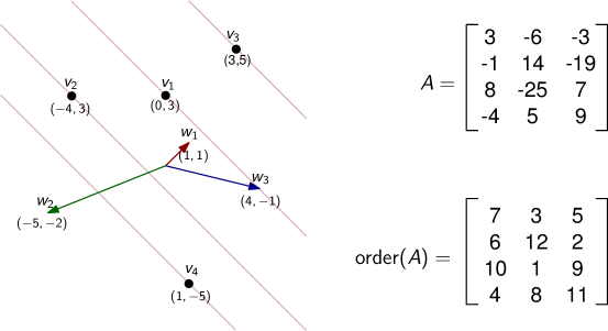
Figure 27: A rank-two representation of the matrix $A$. The points of $V$ are shown as black disks and the points of $W$ are shown as colored vectors. In light red, a hyperplane with normal vector $w_{1}$ is shown sweeping across space. It encounters the points of $V$ in the order $v_{4},v_{2},v_{1},v_{3}$.

Definition 0.26.

A rank-d representation of a matrix $A$ is a set of points

$$v_{1},v_{2},\ldots,v_{m},w_{1},w_{2},\ldots,w_{n}\in\mathbb{R}^{d}$$

and a monotone function $f$ such that $A_{ij}=f(v_{i}\cdot w_{j})$.

See Figure 27 for an example of a rank-2 representation of a matrix.

Example 0.7.

The matrix $A$ has underlying rank at most two.

$$A=\begin{pmatrix}7&3&5\\ 6&12&2\\ 10&1&9\\ 4&8&11\\ \end{pmatrix}$$

This is because the order of entries of $A$ is the same as the order of entries of $B$, which has rank two:

$$B=\begin{pmatrix}3&-6&-3\\ -1&14&-19\\ 8&-25&7\\ -4&5&9\\ \end{pmatrix}$$

A rank-two representation of $A$ is given in Figure 27. We have $w_{1},\ldots,w_{4}$ and $v_{1},\ldots,v_{4}$ given by the rows of the matrices

$$W=\begin{pmatrix}1&1\\ -5&-2\\ 4&-1\\ \end{pmatrix}\qquad V=\begin{pmatrix}0&3\\ -4&3\\ 3&5\\ 1&-5\\ \end{pmatrix}.$$

Notice that the order of entries within the first column corresponds to the order in which a hyperplane normal to the vector $w_{1}$ sweeps past the points $v_{1},v_{2},v_{3},v_{4}$. In Lemma 0.4, we will show that this is always true. Using this result, together with Corollary 0.6, we will show that this matrix has underlying rank exactly two.

As we saw in Example 0.7, we are able to recover a considerable amount of geometric information about the point arrangement $v_{1},\ldots,v_{m}$ using the order of entries of $A$. We can use this information to bound the underlying rank of $A$.

We first notice that the order of entries in each column of a matrix $A$ corresponds to the order in which a sequence of hyperplanes sweep past the points $v_{1},\ldots,v_{m}$ in any rank-$d$ representation of $A$. This is illustrated in Figure 27.

Lemma 0.4.

Let $v_{1},\ldots,v_{m},w_{1},\ldots,w_{n}$, $f$ be a rank-$d$ realization of $A$.

Let $r_{j}(t)$ be the hyperplane defined by $r_{j}(t)=\{w\mid v_{j}\cdot w=t\}$. The order of entries in the $j$-th row of $A$ is equal to the order in which the hyperplane $r_{j}(t)$ encounters the points $w_{1},\ldots,w_{m}$ as we increase $t$.

Likewise, let $c_{i}(t)$ be the hyperplane defined by $c_{i}(t)=\{v\mid w_{i}\cdot v=t\}$. The order of entries in the $i$-th column of $A$ is equal to the order in which the hyperplane $c_{i}(t)$ encounters the points $v_{1},\ldots,v_{m}$ as we increase $t$.

Proof.

Set $t_{ij}$ to be the “time" that $r_{j}(t)$ crosses the point $w_{i}$. That is, $t_{ij}$, $w_{i}\cdot v_{j}=t_{ij}$. The order in which the sweeping hyperplane $r_{i}(t)$ crosses the points $w_{1},\ldots,w_{n}$ is the order of the values of $t_{1j},\ldots,t_{nj}$.

Thus, $v_{j}$ is the $k^{th}$ point the hyperplane $h_{i}(t)$ hits if $t_{ij}$ is the $k^{th}$ smallest value among $t_{1j},\ldots,t_{nj}$. Now, by the definition of a rank $d$ realization, $A_{ij}=f(w_{i}\cdot v_{j})=f(t_{ij})$. Since $f$ is monotone, the values of $A_{ij}=f(t_{ij})$ are in the same order as the values of $t_{ij}$. Thus, the order within the $j^{th}$ row is the same as the order in which the hyperplane $r_{j}(t)$ encounters the points $w_{1},\ldots,w_{m}$ as we increase $t$.

By the same argument, we can show that the order of entries in the $i$-th column of $A$ is equal to the order in which the hyperplane $c_{i}(t)$ encounters the points $v_{1},\ldots,v_{m}$ as we increase $t$.

∎

Corollary 0.6.

If $A$ is a matrix of underlying rank one, then the order of entries in each row of $A$ is either the same as or the reverse of the order of entries in the first row of $A$. Likewise, the order of entries in each column of $A$ is either the same as or the reverse of the order of entries in the first column of $A$.

Proof.

Let $v_{1},\ldots,v_{n},w_{1},\ldots,w_{n},f$ be a rank-one realization of $A$. By Lemma 0.4, the order of entries in the $j$-th row of $A$ is the order in which the hyperplane perpendicular to $v_{j}$ sweeps past the points $w_{1},\ldots,w_{n}$. Since the points $w_{1},\ldots,w_{n}$ are on the real line, there are only two possible orders to sweep past them, one of which is the reverse of the other. ∎

Using Corollary 0.6, we can show that the matrix $A$ in Example 0.7 has underlying rank exactly two. We notice that the order in the second column is neither the same as nor reversed from the order in the first column, thus the underlying rank is greater than one. Since we have already demonstrated that it is as most two by providing a rank two representation, this shows that it is exactly two. As it turns out, $A$ has the highest possible underlying rank for a $3\times 3$ matrix.

Proposition 0.8.

If $A$ is a $n\times n$ matrix, then $\operatorname{urank}(A)\leq n-1$.

Proof.

By the matrix determinant lemma [81](Lemma 1.1), for any ${u},{v}\in\mathbb{R}^{n}$,

$${\displaystyle\det\left(A+{uv}^{\textsf{T}}\right)=\left(1+{v}^{\textsf{T}}A^{-1}{u}\right)\,\det\left(A\right)\,.}$$

Let $\mathbf{1}$ be the all ones vector. Let $\lambda=\mathbf{1}^{\textsf{T}}A^{-1}\mathbf{1}$. Notice that we can perturb $A$ without changing the order of entries so that $\lambda\neq 0$. Now, let $u=\mathbf{1}$, $v=\frac{-1}{\lambda}\mathbf{1}$, $B=A+uv^{\textsf{T}}$. Notice that since $uv^{\textsf{T}}$ is the matrix whose entries are all $-\lambda$, the order of entries in $B$ matches the order of entries in $A$. By the matrix determinant lemma,

$$\det(B)=\left(1+{v}^{\textsf{T}}A^{-1}{u}\right)\,\det\left(A\right)=0.$$

Thus, $B$ is a matrix of rank at most $n-1$ whose entries are in the same order as those of $A$.

∎

In small cases, it is possible for this bound to reach equality: for $n=2,3,4$, we can give examples of $n\times n$ matrices of rank $n-1$. In particular, any $2\times 2$ order matrix has underlying rank at least one, since the only rank-zero matrix is the all zeros matrix, which is not compatible with any strict ordering. In Example 0.7, we gave an example of a $3\times 3$ matrix with underlying rank two. In Example 0.10, we give an example of a $4\times 4$ matrix of underlying rank three. We do not know whether, for all $n$, it is possible for an $n\times n$ matrix to have rank $n-1$.

Minimal nodes: a practical tool to estimate underlying rank

In this section, we introduce the minimal, maximal, and extremal nodes of a matrix. These are the first practical tools we give for estimating the underlying rank.

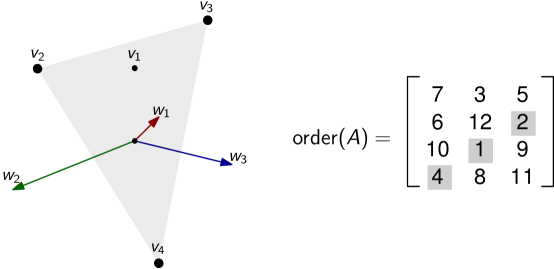
Figure 28: The indices 2, 3 and 4 are minimal for the matrix $A$. These vertices are on the boundary of $\operatorname{conv}(v_{1},v_{2},v_{3},v_{4})$.

Minimal nodes

Minimal, maximal, and extremal nodes are a useful feature for identifying low-rank matrices.

Definition 0.27.

Let $A$ be a $m\times n$ matrix. A row index $i\in[m]$ is a minimal node if $A$ has a column index $j\in[n]$ such that $A_{ij}<A_{kj}$ for all $k\in[m].$ That is, $i$ is minimal if there exists a column $j$ whose smallest entry is in the $i$-th row. An index $i\in[m]$ is a maximal node if $A$ has a column index $j\in[n]$ such that $A_{ij}>A_{kj}$ for all $k\in[m].$ We say $i$ is an extremal node if it is either maximal or minimal.

Extremal nodes capture a feature of the underlying point arrangement: in order to correspond to an extremal node, a point must be a vertex of the convex hull of the full set of points, illustrated in Figure 28.

Definition 0.28.

The convex hull of a set of points $v_{1},\ldots,v_{m}\subset\mathbb{R}^{d}$ is

$$\operatorname{conv}\left(\{v_{j}\}_{j\in[m]}\right)=\left\{\sum_{i=1}^{m}\lambda_{j}v_{j}\,\bigg{\rvert}\,\sum_{j=1}^{m}\lambda_{j}=1,\lambda_{j}\geq 0\right\}$$

Proposition 0.9.

If $i$ is an extremal node of $A$, then $v_{i}$ is a vertex of $\operatorname{conv}(\{v_{j}\}_{j\in[m]})$ for any $v_{1},v_{2},\ldots,v_{m}\in\mathbb{R}^{d}$ rank-$d$ representation of $A$.

Proof.

If $i$ is an extremal node of $A$, then the linear functional $f(x)=w_{j}\cdot x$ is either maximized or minimized on $v_{i}$ among the points $v_{1},\ldots,v_{m}.$ The maximum and minimum values of a linear function on the convex polytope $\operatorname{conv}(\{v_{j}\}_{j\in[m]})$ occur on vertices. Thus, both the maximum and minimum value of $f$ among $v_{1},\ldots,v_{m}$ must occur on a vertex. ∎

Expected numbers of minimal nodes

Because extremal nodes must correspond to vertices of $\operatorname{conv}(v_{1},\ldots,v_{m})$, the expected number of extremal nodes is bounded by the expected number of vertices of a random polytope. As dimension increases, the expected number of vertices increases. Thus, we can use the number of extremal nodes to estimate the underlying rank. One complication is that this expected number of vertices on the convex hull of $m$ random points in $\mathbb{R}^{d}$ depends on the probability distribution used to choose the points. Another complication is that not all vertices are minimal nodes: in particular, if a point arrangement is chosen within the positive orthant, many vertices are prohibited from being minimal nodes.

Expected numbers of vertices

Our first model for a random rank $d$ matrix chooses points $v_{1},\ldots,v_{m}$ uniformly in a unit cube centered at the origin.

Proposition 0.10.

Let $A=f(v_{i}\cdot w_{j})$ be an underlying rank-$d$ matrix whose underlying point arrangement $v_{1},\ldots,v_{m}$ is drawn uniformly at random from the unit cube in $\mathbb{R}^{d}$. Then the expected number $n_{e}$ of extremal nodes is bounded above by

$$\mathbb{E}(n_{e})\leq\frac{2^{d}d}{(d+1)^{d-1}}\log(m)^{d-1}+O(\log(m)^{d-2}\log\log(m))$$

Proof.

Let $\operatorname{Vert}P_{n}$ be the number of vertices of the convex hull of $n$ points samples from the convex polytope $P$. Let $T(P)$ count the number of maximal chains in the face lattice of the polytope. Equation 1.6 of [82] states that

$$\mathbb{E}(\operatorname{Vert}P_{n})=\frac{T(P)}{(d+1)^{d-1}(d-1)!}\log(m)^{d-1}+O(\log(m)^{d-2}\log\log(m))$$

Now, we can count maximal chains in the face lattice of the cube as follows. We an label each face $F$ of the $d$-dimensional cube with a string $X_{f}$ of $d$ zeros, ones, and stars. We define $X_{F}(i)=0$ if $x_{i}$ is constrained to be zero on $F$, $X_{F}(i)=1$ if $x_{i}$ is constrained to be one on $F$, and $X_{f}(i)=*$ if the value of $x_{i}$ varies on $F$. Each maximal chain starts with one of the $2^{d}$ vertices of the cube, which has a string $X_{v}$ with no stars. Now, a chain which starts at $v$ corresponds to an order in which we choose coordinates to replace with stars. Thus, there are $d!$ ways to do this. This comes out to a total of $2^{d}d!$ maximal chains.

Thus, for $d$-dimensional cube $C^{d}$,

$$\mathbb{E}(\operatorname{Vert}C^{d}_{n})=\frac{2^{d}d}{(d+1)^{d-1}}\log(m)^{d-1}+O(\log(m)^{d-2}\log\log(m))$$

Since each minimal node corresponds to a vertex, if $A$ is a random rank $d$ matrix generated from a point arrangement uniformly sampled from the unit cube, the expected number $n_{m}$ of minimal nodes is bounded above by

$$\mathbb{E}(n_{m})\leq\frac{2^{d}d}{(d+1)^{d-1}}\log(m)^{d-1}+O(\log(m)^{d-2}\log\log(m)).$$

∎

We can make similar estimates if the points $v_{1},\ldots,v_{m}$ are chosen according to a Gaussian distribution, using results from [83].

Proposition 0.11.

Let $A=f(v_{i}\cdot w_{j})$ be a random underlying rank-$d$ matrix whose underlying point arrangement $v_{1},\ldots,v_{m}$ is drawn from a Gaussian distribution in $\mathbb{R}^{d}$. Then the expected number $n_{e}$ of extremal nodes is bounded above by

$$\mathbb{E}(n_{e})\leq\beta_{d}\frac{2^{d}}{\sqrt{d}}(\pi\log m)^{(d-1)/2},$$

where $\beta_{d}$ is a constant depending on $d$.

Proof.

By [83], the expected number of vertices of the convex hull of $m$ points drawn from a Gaussian distribution in $\mathbb{R}^{d}$ is asymptotic to $\beta_{d}\frac{2^{d}}{\sqrt{d}}(\pi\log m)^{(d-1)/2},$ where $\beta$ is a constant depending on $d$. By Proposition 0.9, this is an upper bound on the number of minimal nodes. ∎

Proposition 0.12.

Let $A=f(v_{i}\cdot w_{j})$ be an underlying rank-$d$ matrix whose underlying point arrangement $v_{1},\ldots,v_{m}$ is drawn uniformly at random from the unit ball in $\mathbb{R}^{d}$. Then the expected number $n_{e}$ of extremal nodes is bounded above by

$$\mathbb{E}(n_{e})\leq O\left(m^{\frac{d-1}{d+1}}\right)$$

Proof.

By [84], the expected number of vertices of the convex hull of $m$ points sampled uniformly from the unit ball in $\mathbb{R}^{d}$ is $O\left(m^{\frac{d-1}{d+1}}\right)$. By Proposition 0.9, this is an upper bound on the number of minimal nodes. ∎

Notice that the exponent controlling the dependence on $n$ in the Gaussian case is half of that from the uniformly distributed case. Further, the function giving the expected number of vertices in the case of the uniform distribution on a ball is completely different from either of the other distributions. Further, these are just three possible ways of choosing a point arrangement–there is not a finite list of distributions to check. Finally, not all vertices are picked up as minimal nodes. This means that the expected number of vertices gives an upper bound on the number of minimal nodes, based on the dimension. Thus, without information about the underlying probability distribution, we cannot reliably estimate underlying rank from the number of extremal nodes alone. However, with an appropriately chosen family of control distributions, we can estimate the underlying rank by computing the number of minimal nodes and comparing to a control distribution. This control distribution can be chosen based off of the scientific context.

Sign constraints

While every extermal node of the matrix is a vertex of the convex hull, not every vertex of the convex hull actually is observed as an extremal node. This means that features of the distribution generating the underlying point arrangement which do not affect the expected number of vertices can nonetheless affect the number of minimal nodes. In particular, we consider sign constraints: what if we choose points within the positive orthant? We show that this can reduce the number of minimal nodes. More precisely, the number of minimal nodes of a point arrangement contained in the first quadrant is approximately $\frac{1}{2^{d}}$ that of a point arrangement centered at the origin, as exemplified in Figures 29 and 30

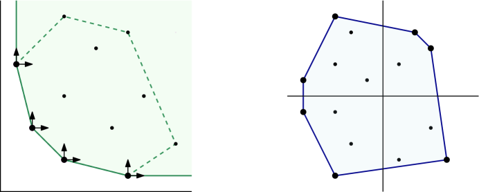
Figure 29: Potential minimal modes for positive (A) and mixed sign (B) point arrangements in $\mathbb{R}^{2}$. Potential minimal nodes are enlarged. On the left, the convex hull of the point arrangement is shown with a dashed line.

Definition 0.29.

A nonnegative rank-$d$ realization of a matrix $A$ is a rank $d$ representation of $A$ with all points in the positive orthant: $v_{1},\ldots,v_{m},w_{1},\ldots,w_{n}\in\mathbb{R}^{d}_{\geq 0}$. The nonnegative underlying rank of a matrix is the smallest value of $r$ for which a nonnegative rank $r$ realization exists.

The next result shows that the minimal and maximal nodes of a nonnegative rank-$d$ realization of a matrix $A$ must meet stricter conditions than merely being vertices. This implies that there are fewer extremal nodes in the mixed-sign case, and that the minimal and maximal nodes are (almost) disjoint. This fact can be used to determine whether a positive or mixed-sign model is more appropriate for a given dataset.

Definition 0.30.

Let $A,B\subset\mathbb{R}^{d}$. The Minkowski sum of $A$ and $B$ is the set

$$A+B=\{a+b\mid a\in A,b\in B\}.$$

Proposition 0.13.

If $i$ is a minimal node of $A$ and $v_{1},\ldots,v_{m},w_{1},\ldots,w_{n}\in\mathbb{R}^{d}$ is a nonnegative rank-$d$ representation of $A$, then $v_{i}$ is a vertex of the polytope

$$\operatorname{conv}(v_{1},\ldots,v_{m})+\mathbb{R}^{d}_{\geq},$$

where the $+$ denotes the Minkowski sum.

If $i$ is a maximal node of $A$ and $v_{1},\ldots,v_{m},w_{1},\ldots,w_{n}\in\mathbb{R}^{d}$ is a nonnegative rank-$d$ representation of $A$, then $v_{i}$ is a vertex of the polytope

$$\operatorname{conv}(v_{1},\ldots,v_{m})+\mathbb{R}^{d}_{\leq}.$$

Proof.

We prove this statement for minimal nodes. The proof of the statement for maximal nodes is analogous.

Let $i$ be a minimal node and $j\in[n]$ such that $A_{ij}<A_{kj}$ for all $k\in[m].$ Equivalently, $v_{i}$ is the point of $v_{1},\ldots,v_{m}$ that minimizes the inner product $v\cdot w_{j}$. On the other hand, by the definitions of convex hull and Minkowski sum, we can write

$$\operatorname{conv}(v_{1},\ldots,v_{m})+\mathbb{R}^{d}_{\geq}=\{\lambda_{1}v_{1}+\cdots+\lambda_{m}v_{m}+x\mid\lambda_{1},\ldots\lambda_{m}\geq 0,\lambda_{1}+\cdots+\lambda_{m}=1,x\in\mathbb{R}^{d}_{\geq 0}\}.$$

This tells us that $v_{i}$ is a vertex of $\operatorname{conv}(v_{1},\ldots,v_{m})$, and

$$w_{j}\cdot v_{i}\leq w_{j}\cdot(\lambda_{1}v_{1}+\cdots+\lambda_{m}v_{m}),$$

whenever $\lambda_{1},\ldots\lambda_{m}\geq 0,\lambda_{1}+\cdots+\lambda_{m}=1$ and that this inequality is strict whenever $\lambda_{i}<1$.

Because $w_{j}$ is in the positive orthant, $w_{j}\cdot x\geq 0$ for all $x$ in the positive orthant. Thus,

$$w_{j}\cdot v_{i}\leq w_{j}\cdot(\lambda_{1}v_{1}+\cdots+\lambda_{m}v_{m}+x),$$

for all $\lambda_{1},\ldots\lambda_{m}\geq 0,\lambda_{1}+\cdots+\lambda_{m}=1,x\in\mathbb{R}^{d}_{\geq 0},$ and this inequality is strict whenever $\lambda_{i}<1$. Thus, $v_{i}$ minimizes the inner product $w_{j}\cdot v$ for all $v\in\operatorname{conv}(v_{1},\ldots,v_{m})+\mathbb{R}^{d}_{\geq}$. Thus, $v_{i}$ is a vertex of $\operatorname{conv}(v_{1},\ldots,v_{m})+\mathbb{R}^{d}_{\geq}$. ∎

Figure 31 collects these calculations for varying $n$. Curves labeled “random full rank” correspond in both cases to randomly generated matrices (non-symmetric) with positive or mixed signed entries, respectively. Notice that in the mixed-sign case there is an overlap between the curves corresponding to (true) random full rank matrices and to the case $d=n$ (gold and aqua curves).

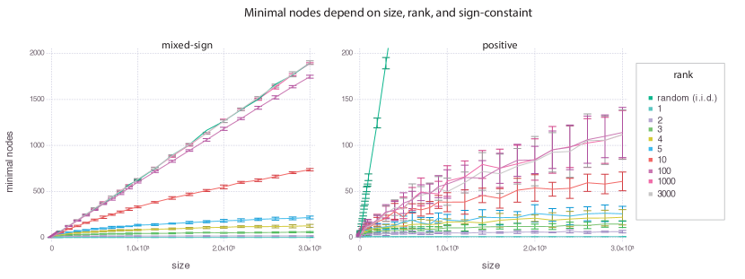
Figure 30: Average number of minimal nodes for samples of 5 matrices, obtained as $BB^{\prime}$, for $B$ an $n\times d$ matrix with random uniformly distributed entries in $[0,1]$ (left, positive) and $[-1/2,1/2]$ (right, mixed-sign). In both cases $d$ is the rank of the resulting matrix $BB^{\prime}$. Curves are color coded by rank. Error bars are given by standard deviations.

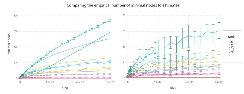
Figure 31: We compare the observed number of minimal nodes to the asymptotic upper bounds appearing in Proposition 0.10 and Conjecture 0.2. In particular, in the mixed sign case, we plot the quantity $\frac{2^{d}d}{(d+1)^{d-1}}\log(m)^{d-1}$ and in the positive case, we plot the quantity $\frac{d}{(d+1)^{d-1}}\log(m)^{d-1}$. We notice that for higher ranks, we underestimate the number of minimal nodes, as the $O(\log(m)^{d-2}\log\log(m))$ correction term matters more in this case.

If $A$ has low non-negative rank, it will have fewer minimal nodes. Roughly, if $A$ is a a random non-negative underlying rank-$d$ matrix whose underlying point arrangement $v_{1},\ldots,v_{m}$ is drawn uniformly at random from the unit cube in the positive orthant, the expected number of minimal nodes is bounded above by $\mathbb{E}(n_{v})/2^{d}$, which in the case of the unit cube is given by $\frac{d}{(d+1)^{d-1}}\log(n)^{d-1}.$ Observe in Figure 31 that this matches up with computational experiments with random matrices. We give a heuristic argument for why this should be the case: in order for $v_{i}$ to be a vertex of $\operatorname{conv}(v_{1},\ldots,v_{n})+\mathbb{R}^{d}_{\geq},$ $v_{i}$ must be a vertex of $\operatorname{conv}(v_{1},\ldots,v_{n})$ whose normal cone intersects the positive orthant. Since the positive orthant in $\mathbb{R}^{d}$ takes up $\frac{1}{2^{d}}$ the volume of the unit cube centered at the origin in $\mathbb{R}^{d}$, the probability that $v_{i}$ is a vertex of $\operatorname{conv}(v_{1},\ldots,v_{n})+\mathbb{R}^{d}_{\geq}$ is roughly $\frac{1}{2^{d}}$ the probability that $v_{i}$ is a vertex of $\operatorname{conv}(v_{1},\ldots,v_{n})$. Thus, the probability that $v_{i}$ is a minimal node of a random positive rank-$d$ matrix is roughly $\frac{1}{2^{d}}$ the probability that $v_{i}$ is a minimal node of a random mixed-sign rank-$d$ matrix. Note that this argument neglects the volume of the normal cone of $v_{i}$, making it a heuristic argument and not a proof. Thus, we leave this as a conjecture:

Conjecture 0.2.

If $v_{1},\ldots,v_{n}$ are drawn uniformly at random from the unit cube $[0,1]^{d}$, then the expected number of minimal nodes is

$$\mathbb{E}(n_{v})/2^{d}=\frac{d}{(d+1)^{d-1}}\log(n)^{d-1}+O(\log(m)^{d-2}\log\log(m)).$$

In Figure 31, we compare the quantity $\frac{d}{(d+1)^{d-1}}\log(n)^{d-1}$ to the observed number of minimal nodes for random matrices of various ranks. We see that for low ranks, the estimate holds, but for high ranks, it does not, likely due to the factor $O(\log(m)^{d-2}\log\log(m)).$

We can interpolate between the mixed-sign and positive case by constraining some, but not all, coordinates to be positive. We define the positivity of a point arrangement as the number of coordinates which are required to be positive. For example, Figure 32 shows how much the overlapping sets differ for $d=2$. As we increase the positivity, we decrease the number of minimal nodes. We also decrease the overlap between minimal and maximal nodes, the number of nodes which are both minimal and maximal. We can use the overlap and positivity together to estimate underlying rank, assuming a distribution for the underlying point arrangement.

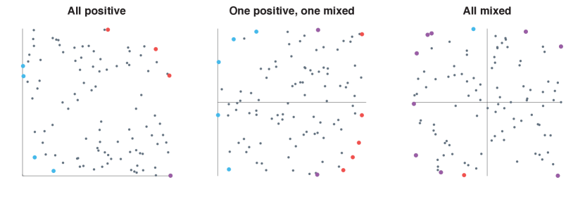
Figure 32: We show the effect of increasing positivity on the number of minimal, maximal, and overlap nodes. In each plot, the minimal nodes are colored blue, the maximal nodes red and the overlapping nodes (nodes that are both minimal and maximal) are colored purple. Notice that in the all-positive case and the one positive, one mixed case the overlap is minimal, whereas in the all-mixed case the overlap consists of most of the nodes.

Matrices with i.i.d entries.

The next proposition shows that we can characterize the expected number of minimal nodes for matrix with independent, identically distributed (i.i.d.) entries. In particular, we show that the expected number of minimal nodes of a square matrix with i.i.d. entries is linear in the matrix size. This allows us to distinguish matrices with some kind of low-rank structure (or other structure) from truly random matrices.

Proposition 0.14.

Let $A$ be a random $n\times n$ matrix with i.i.d. entries. Then

$$\lim_{n\to\infty}\frac{\mathbb{E}\left(|\min(A)|\right)}{n}=\left(1-\frac{1}{e}\right).$$

Proof.

Let $X_{i}$ be a random variable defined by

$$X_{i}=\begin{cases}1\qquad i\in\min(A)\\ 0\qquad\mbox{otherwise}\end{cases}$$

Note that

$$\mathbb{E}\left(|\min(A)|\right)=\mathbb{E}\left(\sum_{i=1}^{n}X_{i}\right)=\sum_{i=1}^{n}\mathbb{E}(X_{i}),$$

since the sum of expected values is always the expected value of the sum. Thus, it is sufficient to calculate $\mathbb{E}(X_{i})$. To do this, define another random variable

$$X_{ij}=\begin{cases}1\qquad i\mbox{ is \emph{not} minimal in row j}\\ 0\qquad\mbox{otherwise}\end{cases}$$

By the assumption that the matrix entries are $i.i.d$, $\mathbb{E}(X_{ij})=\frac{n-1}{n}$ for all $i,j$, since each entry in the $j^{th}$ row has an equal chance of being the smallest.

Now, note that $i$ is minimal if $X_{ij}=0$ for at least one $j$. Thus, $i$ is minimal if and only if $\prod_{j=1}^{n}X_{ij}=0$. Thus $X_{i}=1-\prod_{j=1}^{n}X_{ij}$,

$$\mathbb{E}(X_{i})=1-\mathbb{E}\left(\prod_{j=1}^{n}X_{ij}\right).$$

Again by assumption, $X_{ij}$ and $X_{ik}$ are independent for $j\neq k$. Thus $\mathbb{E}\left(\prod_{j=1}^{n}X_{ij}\right)=\prod_{j=1}^{n}\mathbb{E}(X_{ij})$, so

$$\mathbb{E}(X_{i})=1-\left(\frac{n-1}{n}\right)^{n}=1-\left(1-\frac{1}{n}\right)^{n}.$$

Thus,

$$\mathbb{E}\left(|\min(A)|\right)=\mathbb{E}\left(\sum_{i=1}^{n}X_{i}\right)=n\left(1-\left(1-\frac{1}{n}\right)^{n}\right).$$

By a standard result of calculus, $\lim_{n\to\infty}\left(1-\frac{1}{n}\right)^{n}=\frac{1}{e}$. Thus

$$\lim_{n\to\infty}\frac{\mathbb{E}\left(|\min(A)|\right)}{n}=\left(1-\frac{1}{e}\right).$$

∎

Notice that this proof does not hold for random symmetric matrices. Empirically, however, we have seen that it does hold in this case.

Conjecture 0.3.

Let $A$ be a random $n\times n$ symmetric matrix with the entries above the diagonal i.i.d. Then

$$\lim_{n\to\infty}\frac{\mathbb{E}\left(|\min(A)|\right)}{n}=\left(1-\frac{1}{e}\right).$$

Radon’s theorem: a lower bound for underlying rank

As we saw, extremal nodes can help us estimate the underlying rank of a matrix. However, since a polygon can have an unlimited number of vertices, we cannot use extremal nodes to prove that underlying rank is greater than two. Further, the minimal nodes only capture a very small part of the combinatorial structure of the point configuration $v_{1},\ldots,v_{n}$. In this section, we leverage more of this structure in order to establish lower bounds on underlying rank. We do so by introducing two simplicial complexes, the sweep complex and the shatter complex, whose dimensions give lower bounds for underlying rank that we establish via Radon’s theorem.

The Sweep and Shatter Complexes

In this section, we consider the geometric constraints the ordering of entries in the matrix $A$ place upon rank-$d$ representations of $A$. By Lemma 0.4, the order of entries in each row of $A$ corresponds to the order in which a sequence of hyperplanes sweeps past the points $v_{1},\ldots,v_{m}$. We will use this to build two combinatorial objects, the sweep complex and the shatter complex, which will help us bound the underlying rank. While these invariants are more computationally expensive than minimal nodes, they are able to provide stronger lower bounds.

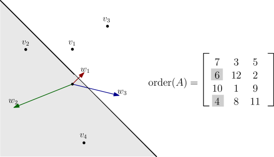
Figure 33: The set $\{2,4\}$ is swept by the first column of $\operatorname{order}(A)$. Consequently, we can deduce that there is a hyperplane separating $\{v_{2},v_{4}\}$ from $\{v_{1},v_{3}\}$.

Definition 0.31.

Let $A$ be a $m\times n$ matrix. A set of columns $\sigma\subseteq[m]$ is swept by $A$ if there is some row $i$ such that:

1. $A_{ij}<A_{ik}$ for all $j\in\sigma,k\notin\sigma$

2. $A_{ij}>A_{ik}$ for all $j\in\sigma,k\notin\sigma$

An example of a swept set appears in Figure 33.

Lemma 0.5.

If a set $\sigma\subseteq[m]$ is swept by $A$, then in any rank-$d$ realization of $A$, there is a hyperplane separating the points $\{v_{i}\}_{i\in\sigma}$ from the points $\{v_{j}\}_{j\notin\sigma}$.

Proof.

Suppose $\sigma$ is swept by the $k$-(th) column of $A$. By Lemma 0.4, the sweeping hyperplane $c_{k}(t)$ encounters all points $\{v_{i}\}_{i\in\sigma}$ before it encounters any of the points $\{v_{j}\}_{j\in[n]\setminus\sigma}$. Let $t_{i}$ be the time such that $v_{i}\in c_{k}(t_{i})$. Thus we can choose $t^{\prime}$ so that $\max_{i\in\sigma}{t_{i}}<t^{\prime}<\min_{j\in[n]\setminus}{t_{j}}$. The hyperplane $c_{k}(t^{\prime})$ separates the points $\{v_{i}\}_{i\in\sigma}$ from the points $\{v_{j}\}_{[n]\setminus\sigma}$.

∎

We now describe two ways to build a simplicial complex out of the set system

$$H_{A}:=\{\sigma\subseteq[m]\mid\sigma\mbox{ is swept by }A\}.$$

First, we define the sweep complex $\Delta_{sw}(A,L)$ with respect to a set of landmarks $L\subseteq[m]$. This is the largest simplicial complex contained in the set $H_{A}\cap L:=\{\sigma\cap L\mid\sigma\in H_{A}\}$. More explicitly,

$$\Delta_{sw}(A,L)=\{\sigma\mid\tau\in H_{A}\cap L\mbox{ for all }\tau\subseteq\sigma\}$$

Notice that the vertex set of $\Delta_{sw}(A,L)$ is the set of minimal nodes contained in $L$. More generally, we will see that the faces of $\Delta_{sw}(A,L)$ are faces of the convex polytope $\operatorname{conv}(\{v_{i}\mid i\in L\})$. In this sense, the sweep complex is the most natural way to give a structure to the set of minimal nodes. We typically choose $L$ to be a small, proper subset of the minimal nodes of $A$. Picking $L$ to be smaller not only speeds up computation, but also loosens the conditions required to include a simplex $\sigma\in\Delta_{sw}(A,L)$, increasing the rank we detect. The sweep complex is inspired by the witness complex of [85].

Next, we define the shatter complex $\Delta_{sh}(A)$. We say $\sigma\subseteq[m]$ is shattered by $H_{A}$ if for all $\tau\subseteq\sigma$, there exists $\omega\in H_{A}$ such that $\tau=\sigma\cap\omega$. The shatter complex is

$$\Delta_{sh}(A)=\{\sigma\mid\sigma\mbox{ is shattered by }H_{A}\}.$$

Notice that for any $L$, $\Delta_{sw}(A,L)\subseteq\Delta_{sh}(A)$. We will show that each simplex of the shatter complex corresponds to an affinely independent subset of the points $v_{1},\ldots,v_{m}$. We will establish this using a version of Radon’s theorem.

Notice that there is a hyperplane separating the points $\{v_{i}\mid i\in\sigma\}$ from the $\{v_{i}\mid j\in\tau\}$ if and only if $\operatorname{conv}(\{v_{i}\mid i\in\sigma\})\cap\operatorname{conv}(\{v_{i}\mid j\in\tau\})=\varnothing$.

Lemma 0.6.

(Radon’s theorem) A set of points is affinely independent if for every partition $\sigma,\tau$ of the points, they points in $\sigma$ and the points in $\tau$ can be separated by a hyperplane.

Proposition 0.15.

Let $A$ be a $m\times n$ matrix with underlying point arrangement $v_{1},\ldots,v_{m}$. Then if $\omega\in\Delta_{sh}(A)$, the set $\{v_{i}\mid i\in\omega\}$ is affinely independent.

Proof.

Suppose $\omega\in\Delta_{sh}(A)$. Then for each partition $\sigma\cup\tau=\omega$, $\sigma\cap\tau=\varnothing$, both $\sigma$ and $\tau$ are intersections $\sigma=h\cap\omega$, $\tau=h^{\prime}\cap\omega$ for some $h,h^{\prime}\in H_{A}$. Thus there is a hyperplane separating the points $\{v_{i}\mid i\in\sigma\}$ from the points $\{v_{j}\mid j\in\tau\}$. Thus, the set of points $\{v_{i}\mid i\in\sigma\}$ has no Radon partition. Thus, it is affinely independent. ∎

An affinely independent set in $\mathbb{R}^{d}$ has at most $d+1$ points. Thus, the dimension of the sweep complex is a lower bound on underlying rank. Inspired by Radon’s theorem, we term this the Radon rank $\operatorname{radrank}(A)$.

Proposition 0.16.

The Radon rank of a matrix is a lower bound on its underlying rank. That is,

$$\operatorname{radrank}(A)\leq\operatorname{urank}(A).$$

A similar bound can be derived from the sweep complex, however, this requires slightly more casework. Further, this cannot exceed the Radon rank.

The Radon rank closely resembles the concept of the Vapnik–Chervonenkis (VC) dimension from statistical learning theory [86]. The VC dimsnion of a set system $H$ is the size of the largest set shattered by $H$. Thus, Radon rank of a matrix $A$ is the VC dimension of the set system $H_{A}$, minus one. Similar ideas have been used to estimate the dimensionality of neural activity in [87].

How high can Radon rank be?

The Radon rank is not equal to either the underlying rank or the monotone rank in general. In particular, we see in the next proposition that the the size of the smallest matrix with Radon rank $d$ is exponential in $d$. This is due to a combinatorial explosion in the number of column orders needed to shatter a simplex.

Proposition 0.17.

The Radon rank $d=\operatorname{radrank}(A)$ of a $m\times n$ matrix $A$ satisfies

$$\frac{1}{2}\binom{d+1}{\lfloor(d+1)/2\rfloor}\leq n.$$

A plot of this bound appears in Figure 34.

Proof.

If $\operatorname{radrank}(A)=d$, $A$ shatters a set $\rho$ with $|\rho|=d+1$. Thus, for each $\sigma\subseteq\rho$, the set $\sigma$ is swept by $A$. Each column of $A$ sweeps two nested sequences of sets, $\varnothing\subseteq\sigma_{1}\subseteq\cdots\subseteq\\ sigma_{d}\subseteq\rho$ and $\varnothing\subseteq\tau_{1}\subseteq\cdots\subseteq\tau_{d}\subseteq\rho.$ These are chains in the Boolean lattice, the partially ordered set whose elements are subsets of $\rho$ ordered by set-inclusion. In order to induce every partition of $\rho$, these chains must cover the Boolean lattice on $\rho$. Dilworth’s theorem [88] states that the minimal number of chains needed to cover a poset $P$ is exactly equal to the length of the longest antichain of $P$. Sperner’s theorem [89] states that the longest antichain of the Boolean lattice on $k$ elements has length $\binom{k}{\lfloor k/2\rfloor}$. Thus, the number of permutations needed to induce all partitions of $\rho$ is $\binom{d+1}{\lfloor(d+1)/2\rfloor}$. Since each column induces two permutations, we have $\frac{1}{2}\binom{d+1}{\lfloor(d+1)/2\rfloor}\leq n$, as desired. ∎

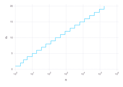
Figure 34: The maximum underlying rank $d$ detectable by an $n\times n$ matrix, plotted as a function of $n$. Note that the scale for $n$ is logarithmic.

Application: dimensionality of neural activity in the larval zebrafish optic tectum

As a proof of concept, we apply the techniques developed here to estimate the underlying rank of a neural dataset. The data consists of calcium imaging of $N=2042$ neurons in the optic tectum of a larval zebrafish obtained from the Sumbre lab at École Normale Supérieure. The recording is one hour long. The zebrafish is in the dark for the duration of the recording, thus the recorded activity is spontaneous, rather than stimulus driven. The sampling rate is 15 Hz. This means the dataset is a $54000\times 2042$ matrix $A$. To reduce noise, we smoothed the data by averaging the activity of each neuron over a sliding window of 2 seconds (30 time bins), producing a matrix $A_{smooth}$.

To get an estimate of the linear dimensionality of our data, we compute the singular values of $A$ and $A_{smooth}$, plotted in Figure 35. Notice that for both $A$ and $A_{smooth}$, the singular values decay smoothly with dimension, following a roughly power law relationship between singular value and dimension. The singular values of $A_{smooth}$ decay faster.

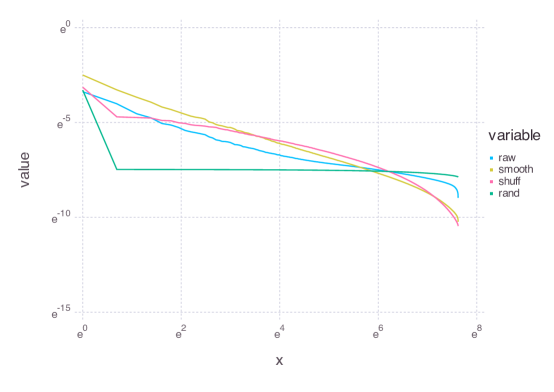
Figure 35: Singular values of the data matrix, before and after smoothing.

However, the monotone nonlinear relationship between firing rate and calcium fluorescence may affect this measure of dimensionality. Thus, we use the concepts we have introduced in this paper to determine whether the ordering of the entries of this matrix is consistent with the estimate of underlying rank based on singular values, or whether it is consistent with a lower rank.

Because differences between low values of calcium fluorescence do not reflect anything meaningful, while differences between high values does, we focus on maximal nodes, rather than minimal nodes. We sample square submatrices of $A_{smooth}$ and count the number of maximal nodes that each one has. We then repeat this process with random matrices of ranks 1, 5, and 10. We plot the results of this in 36. Notice that, in the real data, there is a distinction between maximal rows and maximal columns. In particular, a maximal row corresponds to a time point $t$ where some neuron $i$ achieves its maximal value. On the other hand, a maximal column correspond to a neuron $i$ which is the most active neuron at some time point $t$.

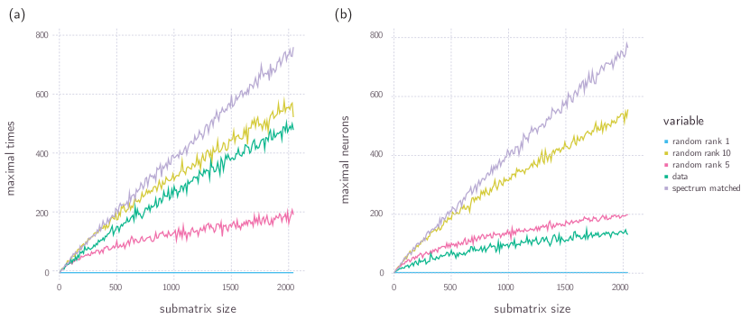
Figure 36: (a) maximal timepoints (b) maximal neurons

Notice in Figure 36, based on the maximal rows (maximal times), the data is most consistent with underlying rank 10, while based on maximal columns (maximal neurons), the data is most consistent with underlying rank 5.

Next, in Figure 37, we use the concept of Radon rank to estimate the underlying rank of $A_{smooth}$. The exact Radon rank of a matrix of this size is prohibitively inefficient to compute, and subject to localized noise, since one set of size $k+1$ being shattered is enough to ensure Radon rank is at least $k$. Therefore, we estimate Radon rank through random sampling and comparison. Since there are more time points than neurons, it is possible to estimate Radon rank over a higher range by sampling sets of $k+1$ neurons and checking whether each possible partition of the neurons is achieved by a row. With the size of the matrix, the highest possible Radon rank which can be detected is 18. Therefore, for each $k=2,3,\ldots,19$, we sampled 100 sets of $k$ neurons and checked which subsets were shattered. For the data matrix, as well as low-rank controls, we plot the fraction of sets which were shattered for each $k$ in Figure 37.

In contrast with minimal nodes, this result is consistent with the singular values of the matrix, and is not consistent with a lower rank. In particular, the data shatters some sets of 13 neurons, establishing a Radon rank of at least 12. The fraction of sets shattered as a function of $k$ most closely resembles a random rank 20 matrix, and is also very similar to that of a singular value-matched control.

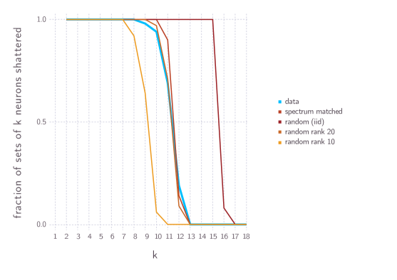
Figure 37: Fraction of sets of size $k$ shattered as a function of $k$.

Conclusion and Open Questions

In Section Minimal nodes: a practical tool to estimate underlying rank, we show that the number of minimal nodes of a random matrix increases as we increase rank, thus that the number of minimal nodes can be used as an order invariant for estimating underlying rank. However, the precise dependence of the number of minimal nodes on rank depends on the probability distribution used to choose our random matrix. Thus, in order to obtain reliable estimates of the underlying rank of a matrix arising from neural data using minimal nodes, we need a biologically realistic way to simulate neural activity with a specified rank.

Question 0.15.

Give a biologically plausible model for random matrices of each rank, and characterize the relationship between rank and minimal nodes from this model.

Further, often data does not have an idealized low rank + noise structure. Instead, singular values decay more smoothly, but it is still often reasonable to regard the data as low rank.

Question 0.16.

Characterize the minimal nodes of matrices with a wider variety of spectra.

The Geometry of Underlying Rank

Introduction

In the previous chapter, we introduced the concept of underlying rank and introduced two tools for estimating it, minimal nodes and Radon rank. In this chapter, we explore the concept of underlying rank in more mathematical detail, show that underlying rank may exceed these estimates, and show that it is difficult to compute exactly. Each of these examples and results arises from the connection between underlying rank and oriented matroid theory.

We begin by describing the relationship underlying rank and three closely related concepts: monotone rank, sign rank, and convex sensing. In particular, the connection to sign rank gives us the following result:

Theorem 0.5.

For each $N=2^{n}$, $O(H_{n})$ is a $N\times N$ order matrix with

$$\operatorname{urank}(O(H_{n}))\geq\sqrt{N}-1.$$

Combined with Proposition 0.17, this implies that underlying rank can exceed Radon rank. Motivated by this, we give three explicit, small examples of matrices whose underlying rank exceeds their Radon rank. These appear in Example 0.8, Proposition 0.19, and Example 0.10. In particular, Proposition 0.19 demonstrates that the set of potential Radon partitions must have a certain structure. In order to generalize this, we relate underlying rank to oriented matroid theory via the following result.

Theorem 0.6.

Suppose $A$ has underlying rank $d$. Then the potential radon partitions of rank $d+1$ of $A$ contain the circuits of a representable oriented matroid of rank $d+1$.

Next, in Example 0.10, we give an example of a matrix for which the detailed column orders contain information beyond the set of Radon partitions. This example arises from a connection underlying rank and allowable sequences. In particular, we note in Observation 0.2 that if a matrix has underlying rank 2, then its columns are contained in a subsequence of an allowable sequence. We use this connection to give an approximate algorithm for determining whether a matrix has underlying rank 2, whose correctness is proven in Proposition 0.21. Further, we exploit the connection between underlying rank and allowable sequences to prove that computing underlying rank is hard.

Theorem 0.7.

Checking whether a matrix has underlying rank two is $\exists\mathbb{R}$-complete and thus NP-hard.

This chapter is organized as follows: First, in Section Mathematical context, we introduce the underlying rank in a mathematical context, comparing it to other similar notions. Next, in Section Improving upon Radon rank using the structure of Radon partitions, we give an explicit example of a matrix whose underlying rank exceeds its Radon rank because the set of possible Radon partitions is not consistent. In Section The combinatorial geometry of underlying rank, we generalize this example using oriented matroid theory.

Mathematical context

In this section, we place the concept of underlying rank in its mathematical context though comparison to three related problems: monotone rank, convex sensing, and sign rank.

Monotone rank

In Lemma 0.4, we proved that the order of entries in the $j$-th column of a matrix $A$ corresponds to the order in which a hyperplane swept perpendicular to $w_{j}$ sweeps past the points $v_{1},\ldots,v_{m}$ in a rank $d$ realization of $A$. Notice that this proof does not depend on the monotone function $f$ being the same for each column. That is, we can replace the global function $f$ with functions $f_{1},\ldots,f_{n}$ such that $A_{ij}=f_{j}(v_{i}\cdot w_{j})$. This fact is used in [90] to define the monotone rank of a matrix. Like underlying rank, monotone rank was introduced in the context of mathematical neuroscience. It makes sense to consider the monotone rank, rather than the underlying rank when the biological context means that each column is distorted in a different way.

Definition 0.32.

The monotone rank of $A$, written $\operatorname{mrank}(A)$, is the smallest value of $d$ such that there exists a rank-$d$ matrix $B$ and a set of monotone functions $f_{1},\ldots,f_{n}$ such that $A_{ij}=f_{j}(B_{ij})$.

Notice that the monotone rank depends only on the ordering of entries within columns of the matrix, while the underlying rank depends on the complete ordering of matrix entries. Further, notice that monotone rank of both $A$ and $A^{T}$ is a lower bound on underlying rank: for any matrix $A$, $\operatorname{mrank}(A)\leq\operatorname{urank}(A)$ and $\operatorname{mrank}(A^{T})\leq\operatorname{urank}(A)$. However, we will see in Example 0.8 that monotone rank of a matrix can be strictly lower than its underlying rank. To develop this example, we use a simple characterization of matrices which have monotone rank one noted in [90]: a matrix $A$ has monotone rank one if and only if there is some order such that every column is either in this order or the reverse order.

Example 0.8.

Consider the matrix

$$A=\begin{pmatrix}1&3&4\\ 2&5&8\\ 6&7&9\\ \end{pmatrix}$$

We first note that $\operatorname{mrank}(A)=1$ because each column of $A$ is in the same order, increasing from top to bottom. However, we prove that $\operatorname{urank}(A)=2$.

Suppose to the contrary that $\operatorname{urank}(A)=1$. Then there exists a rank-one matrix $B$ whose entries are in the same order as the entries of $A$. In rank one, the inner product reduces to scalar multiplication, and thus $B$ is rank one if and only if there exist real numbers $v_{1},v_{2},v_{3}$ and $w_{1},w_{2},w_{3}$ such that $B_{ij}=w_{i}v_{j}$

We can choose these real numbers to be positive. To see this, first notice that because all rows are in the same order, the points $w_{1},w_{2},$ and $w_{3}$ must all have the same sign. We can choose this sign to be positive, flipping the signs on $v_{1},v_{2},v_{3}$ to compensate if necessary. Now, once we have fixed $w_{1},w_{2},w_{3}>0$, we notice that adding a constant shift to the $v_{1},v_{2},v_{3}$ to ensure that $v_{1},v_{2},v_{3}>0$ does not change the ordering among the products $v_{i}w_{j}$. Thus, without loss of generality, we can choose $v_{1},v_{2},v_{3}>0$.

This allows us to replace each entry with its logarithm. Since the logarithm is a monotone increasing function, this does not change the ordering of matrix entries. Thus, the matrix $C$ defined by $C_{ij}=\log(w_{i}v_{j})=\log(w_{i})+\log(v_{j})$ has the same ordering as the original matrix $A$ and the rank-one matrix $B$. To simplify notation, denote $w_{i}^{\prime}=\log(w_{i})$, $v_{i}^{\prime}=\log(v_{i})$. Now, we derive some additional inequalities from the inequalities in the matrix:

From $A_{21}<A_{12}$ and $A_{31}>A_{22}$, we have

$$w_{2}^{\prime}+v_{1}^{\prime}<w_{1}^{\prime}+v_{2}^{\prime}$$

$$w_{3}^{\prime}+v_{1}^{\prime}>w_{2}^{\prime}+v_{2}^{\prime}$$

Subtracting, we have the inequality

$$w_{2}^{\prime}-w_{3}^{\prime}<w_{1}^{\prime}-w_{2}^{\prime}.$$

On the other hand, from $A_{13}<A_{22}$ and $A_{23}>A_{32}$, we have

$$w_{1}^{\prime}+v_{3}^{\prime}<w_{2}^{\prime}+v_{2}^{\prime}$$

$$w_{2}^{\prime}+v_{3}^{\prime}>w_{3}^{\prime}+v_{2}^{\prime}$$

Subtracting, we have the inequality.

$$w_{1}^{\prime}-w_{2}^{\prime}<w_{2}^{\prime}-w_{3}^{\prime}.$$

Thus, we have arrived at a contradiction.

Thus, the underlying rank of $A$ is at least two, even though the monotone rank is one. This means $\operatorname{urank}(A)>\operatorname{mrank}(A)$. This argument can be generalized using Farkas lemma from linear programming. There is a general characterization of matrices of underlying rank one using this idea [91].

Despite the simple characterization of matrices of monotone rank one, we show in Section The combinatorial geometry of underlying rank that characterizing matrices of monotone rank two or higher exactly is computationally intractable. On the other hand, if the rows of $A$ contain the complete set sweeping orders of $v_{1},\ldots,v_{m}$, and we know that this is indeed the complete set, then it is in principle easy to recover the monotone rank of $A$. See [92] for an in depth exploration of this set of sweeping orders as a combinatorial object.

However, we do not expect our data sets to contain this complete set of permutations. The authors of [90] consider the problem of determining monotone rank in this more limited condition. They show that techniques using directed complexes are effective at estimating monotone rank when the number of sweep orders $n$ is much greater than $d$ and techniques using the Dowker complexes are effective at estimating monotone rank when the number of points being swept past $m$ is much greater than $d$.

Sign rank

Finally, underlying rank is closely related to the concept of sign rank, used in theoretical computer science [93, 94, 95]. The relationship between sign rank and underlying rank is illustrated in Figure 38.

Definition 0.33.

The sign rank of a matrix $A$ is the minimum rank of a matrix with the same sign-pattern as $A$:

$$\mathrm{sign\,rank}(A)=\min\{\operatorname{rank}(B):\operatorname{sign}(A_{ij})=\operatorname{sign}(B_{ij})\mbox{ for all }i,j\}$$

Since the only information the sign rank preserves about a matrix is its sign pattern, we typically consider the sign ranks of matrices with entries $\pm 1$, which we term sign matrices. We can relate each order matrix to a family of sign matrices. This will allow us to bound underlying rank of a matrix in terms of the sign rank. In particular, this allows us to show that there is a family of $N\times N$ matrices with underlying rank on the order of $\sqrt{N}$ for all $N=2^{n}$. For large enough $n$, this exceeds all other bounds we give for underlying rank in this paper.

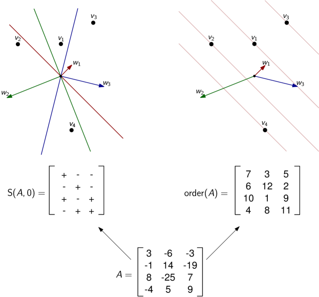
Figure 38: The information carried by the signs of a matrix as compared to the order. On the left, $S(A,0)_{ij}$ indicates which side of the hyperplane perpendicular to $w_{i}$ through the origin the point $v_{j}$ falls on.

Definition 0.34.

Let $A$ be an $m\times n$ matrix, $\theta\in\mathbb{R}$. Then define the sign matrix of $A$ at threshold $\theta$ to be the matrix

$$S(A,{\theta})_{ij}=\operatorname{sign}(A_{ij}-\theta).$$

We use the convention that if $A_{ij}-\theta=0,$ then $S(A,{\theta})_{ij}=-1$.

Notice that the matrix $S(A,{\theta})$ can only change when $\theta$ passes through some $A_{ij}$. Thus for each matrix $A$ there are at most $mn$ sign matrices which arise as $S(A,{\theta})$. We can put all of these matrices together into one matrix.

Definition 0.35.

Define the matrix

$$S(A)=\begin{pmatrix}\operatorname{sign}(A,A_{11})\\ \operatorname{sign}(A,A_{12})\\ \vdots\\ \operatorname{sign}(A,A_{nn})\end{pmatrix}$$

That is, $S(A)$ is the matrix obtained by vertically stacking all of the matrices $\operatorname{sign}(A,A_{ij})$.

We show that sign rank is bounded in terms of underlying rank.

Proposition 0.18.

For all matrixes $A$, $\theta\in\mathbb{R}$, $\operatorname{sign}\operatorname{rank}(S(A,\theta))\leq\operatorname{sign}\operatorname{rank}(S(A))\leq\operatorname{urank}(A)+1$

Proof.

We prove the first inequality, $\operatorname{sign}\operatorname{rank}(S(A,\theta))\leq\operatorname{sign}\operatorname{rank}(S(A)).$
First we look at the case where $\theta>\max_{i,j}A_{ij}$. Here, $S(A,\theta)$ is the all ones matrix, which has sign-rank one. Thus, because $S(A)$ has at least sign rank one, we have $\operatorname{sign}\operatorname{rank}(S(A,\theta))\leq\operatorname{sign}\operatorname{rank}(S(A)).$ Now, for all $\theta\leq\max_{i,j}A_{ij}$, $S(A,\theta)$ is a submatrix of $S(A)$, hence $\operatorname{sign}\operatorname{rank}(S(A,\theta))\leq\operatorname{sign}\operatorname{rank}(S(A)).$

Now, we show the second inequality, $\operatorname{sign}\operatorname{rank}(S(A))\leq\operatorname{urank}(A)+1.$ Let the underlying rank of $A$ be $r$. Let $B$ be a rank-$r$ matrix and $f$ be a monotone function such that

$$A_{ij}=f(B_{ij}).$$

Now, for each $\theta$, observe that $B_{\theta}:=B-f^{-1}(\theta)J$, where $J$ is the all-ones matrix, matches the sign pattern of $S(A,\theta)$. Thus, the matrix

$$\begin{pmatrix}B_{A_{11}}\\ B_{A_{12}}\\ \vdots\\ B_{A_{nn}}\end{pmatrix}=\begin{pmatrix}B\\ B\\ \vdots\\ B\end{pmatrix}-\begin{pmatrix}f^{-1}(A_{11})J\\ f^{-1}(A_{12})J\\ \vdots\\ f^{-1}(A_{nn})J\end{pmatrix}$$

matches the sign pattern of $S(A).$ The matrix $[B\enspace B\enspace\cdots\enspace B]$ is rank $R$, and can thus be written as a sum of $r$ rank one matrices. The matrix $[f^{-1}(A_{11})J\enspace f^{-1}(A_{12})J\enspace\cdots\enspace f^{-1}(A_{nn})J]$ is rank one. Thus we have shown that $B_{\theta}$ can be written as a sum of $r+1$ rank-$r$ matrices, and thus has rank at most $r+1$. Thus, $\operatorname{sign}\operatorname{rank}(S(A))\leq\operatorname{urank}(A)+1.$ ∎

Thus we can apply known results about sign rank to establish lower bounds on underlying rank. We focus on results which bound the sign rank of a sign matrix $M$ in terms of $||M||$. Recall that for any matrix $M$, $||M||=\sigma_{1}(M)$, where $\sigma_{1}(M)$ is the greatest singular value of $M$. This is equal to the square root of the top eigenvalue of $M^{T}M.$

Theorem 0.8.

[94] Let $M\in\{\pm 1\}^{m\times n}$ be a sign matrix of sign rank $d$. Then

$$d\geq\frac{mn}{||M||}.$$

Using this together with Proposition 0.18, we can bound the underlying rank of $A$ in terms of the singular values of $S(A,\theta)$.

Corollary 0.7.

Let $A\in\mathbb{R}^{m\times n}$. Then

$$\operatorname{urank}(A)\geq\frac{mn}{||S(A)||}-1.$$

The cited theorem, and related results, make it possible to construct explicit examples of matrices with high sign rank relative to their size. The primary example given in [94] is the family of Hadamard matrices $H_{n}$. The Hadamard matrices are a family of symmetric matrices with entries $\pm 1$ whose rows are pairwise orthogonal. They are defined recursively, with

$$H_{0}=(1),$$

and

$$H_{n+1}=\begin{pmatrix}H_{n}&H_{n}\\ H_{n}&-H_{n}\end{pmatrix}.$$

Notice that $H_{n}$ is $2^{n}\times 2^{n}$. Let $N:=2^{n}$, so that $H_{n}$ is $N\times N$. Now, we find $||H_{n}||$. Now, because the columns of $H_{n}$ are pairwise orthogonal and the entries are $\pm 1$, we note that

$$H_{n}^{T}H_{n}=NI.$$

This has eigenvalues $N,\ldots,N$. Thus, $||H_{n}||=\sqrt{N}$. Thus, we have

$$\operatorname{sign}\operatorname{rank}(H_{n})\geq\frac{N}{\sqrt{N}}=\sqrt{N}.$$

We can also use the Hadamard matrices to construct examples of matrices with high underlying rank. To do this, we notice that given any sign matrix $S$, we can produce an order matrix $O(S)$, such that $\operatorname{sign}\operatorname{rank}(S)\leq\operatorname{urank}(O(S))+1$. Let $S$ be a $m\times n$ matrix with $N$ negative entries. To produce $O(S)$, we loop through the entries of $S$. If $S_{ij}=-1$, we set $O(S)_{ij}$ to be an element of $1,\ldots,N$. If $S_{ij}=1$, we set $O(S)_{ij}$ to be an element of $N+1,\ldots,mn$. We make sure each value is only used once. Notice that $S=\operatorname{sign}(O(S),N)$, thus $\operatorname{sign}\operatorname{rank}(S)\leq\operatorname{urank}(O(S))+1$. Using this construction, we have

Theorem 0.1.

For each $N=2^{n}$, $O(H_{n})$ is a $N\times N$ order matrix with

$$\operatorname{urank}(O(H_{n}))\geq\sqrt{N}-1.$$

In general, sign rank is difficult to compute: it is complete for the existential theory of the reals, written $\exists\mathbb{R}$. This is the complexity class of decision problems of the form

$$\exists(x_{1}\in\mathbb{R})\cdots\exists(x_{n}\in\mathbb{R})P(x_{1},\ldots,x_{n}),$$

where P is a quantifier-free formula whose atomic formulas are polynomial equations and inequalities in the $x_{i}$ [53]. Many classic problems in computational geometry fall into $\exists\mathbb{R}$ [54]. Problems which are $\exists\mathbb{R}$-complete are not believed to be computationally tractable. In particular, they must be NP-hard. The fact that sign rank is $\exists\mathbb{R}$ complete is established in [95] and independently in [96]. More precisely, for $r\geq 3$, the decision problem of determining whether a matrix $A$ has sign rank $r$ is $\exists\mathbb{R}$-complete.

Note that the fact that computing sign rank is $\exists\mathbb{R}$ complete does not immediately establish that underlying rank is $\exists\mathbb{R}$ complete. However, we will show in Section The combinatorial geometry of underlying rank that underlying rank and monotone rank are also $\exists\mathbb{R}$ complete problems.

Convex sensing

Another related problem is the convex sensing problem introduced in [97]. This problem considers a point arrangement $w_{1},\ldots,w_{n}\subseteq\mathbb{R}^{d}$. The only information we have about this point arrangement is the matrix

$$M_{ij}=f_{i}(w_{j}),$$

where each $f_{i}$ is a quasi-convex function. That is, $f_{i}$ is a function which has convex sublevel sets, i.e. for each threshold $\theta$, $f^{-1}(-\infty,\theta)$ is either convex or empty.

In essence, in the monotone rank and underlying rank problems, we learn about a point configuration by sweeping hyperplanes past it and noticing when the hyperplane passes each point. In the convex sensing problem, we learn about a point configuration by growing convex sets and noticing the order in which each set envelops each point. To obtain the monotone rank problem from the convex sensing problem, we restrict from quasi-convex functions to “quasi-linear functions": functions whose sublevel sets are half-spaces.

This restriction fundamentally changes the problem: while we will show that there exist matrices with arbitrarily high underlying rank, by Corollary 1.5 of [97], any convex sensing problem has a degenerate solution in $\mathbb{R}^{2}$. Thus, [97] takes a probabilistic perspective, focusing on estimating dimension under assumptions about the probability distribution generating the points $w_{1},\ldots,w_{n}$. Some techniques introduced in this paper apply to the convex sensing problem as well. In particular, since a quasi-convex function takes its maximum value on a convex set on the boundary, the maximal nodes we introduced in Section Minimal nodes: a practical tool to estimate underlying rank are also respected by quasi-convex functions. This means that the estimation techniques introduced in this section apply to this problem as well.

Improving upon Radon rank using the structure of Radon partitions

Combining Proposition 0.17 with Theorem 0.1, we see that underlying rank can exceed the Radon rank. Theorem 0.1 gives a family of matrices whose underlying rank scales with the square root of their size, while Proposition 0.17 shows that Radon rank cannot grow this fast. We next consider an explicit example where underlying rank exceeds Radon rank because the possible Radon partitions are not consistent with one another.

A matrix $A$ has Radon rank $d$ if there is a set of size $d+1$ with no possible Radon partition, i.e. partition $(\sigma,\tau)$ not induced by $A$. However, it is possible for every set of size $d+2$ to have a possible Radon partition, but for the underlying rank to still be greater than $d$.

Proposition 0.19.

The inequality in Proposition 0.16 may be strict. In particular, the order matrix

$$A=\begin{pmatrix}12&13&3&10&6\\ 13&14&4&9&5\\ 3&4&15&11&1\\ 10&9&11&8&2\\ 6&5&1&2&7\\ \end{pmatrix}$$

has Radon rank two and monotone rank three.

Proof.

To see this, we first compute the shatter complex of $A$:

$$\Delta_{\mathrm{sh}}(A)=\Delta(123,124,125,134,135,145,234,235,245,345).$$

Since the largest sets of points we can shatter have size $3$, $\operatorname{radrank}(A)=2$. Now, we show that the monotone rank is, in fact, 3.

We suppose for the sake of contradiction that $\operatorname{urank}(A)=2$. Let $v_{1},\ldots,v_{m},w_{1},\ldots,w_{n}\subset\mathbb{R}^{2}$ be a rank-2 representation of $A$. By Radon’s theorem, every subset of $v_{1},\ldots,v_{m},$ of size 4 must has a Radon partition. If $(\sigma,\tau)$ is a Radon partition of $\rho$, then there is no hyperplane separating the sets $\{v_{i}\}_{i\in\sigma}$ and $\{v_{j}\}_{j\in\tau}$. Thus, the partition $(\sigma,\tau)$ must not be induced by $A$.

For each subset of size 4, we compute the set of potential Radon partitions, which are the sets $\sigma,\tau$ such that $\sigma$ and $\tau$ are not swept by $A$. We find that there is exactly one potential Radon partition for each subset:

$$1234:(14,23)$$

$$1235:(1,235)$$

$$1425:(14,25)$$

$$1345:(135,4)$$

$$2345:(235,4)$$

Now, suppose $V$ is an arrangement of points with these Radon partitions, as illustrated in Figure 39. Then the partition $(1,235)$ implies that $v_{1}\in\operatorname{conv}(v_{2},v_{3},v_{5})$. The partition $(14,25)$ implies that the line segment from $v_{1}$ to $v_{4}$ crosses out of the triangle $\operatorname{conv}(v_{2},v_{3},v_{5})$ by crossing the line segment from $v_{2}$ to $v_{5}$. However, the partition $(14,23)$ implies that the line segment from $v_{1}$ to $v_{4}$ crosses out of the triangle $\operatorname{conv}(v_{2},v_{3},v_{5})$ by crossing the line segment from $v_{2}$ to $v_{3}$. Thus, we have reached a contradiction.

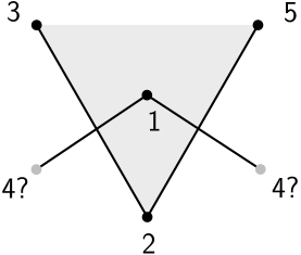
Figure 39: We reach a contradiction when we try to construct a rank two realization of $A$.

In the next section, we generalize this obstruction by exploring the connection between underlying rank and oriented matroid theory.

∎

The combinatorial geometry of underlying rank

In this section, we see how two combinatorial abstractions of point arrangements, oriented matroids and allowable sequences, can inform our understanding of underlying rank. This will get us three main benefits: first, we will generalize the argument made in Proposition 0.19 by describing the structure the minimal Radon partitions of a set of points must have. Second, we will show that for $d\geq 2$, deciding whether a matrix has monotone rank $d$ is complete for the existential theory of the reals, and is therefore NP-hard. Contrary to this, we give a necessary condition for a matrix to have monotone rank 2 which can be checked in $O(mn^{2})$ for a $m\times n$ matrix.

Oriented matroids

We can recast the example in the proof of Proposition 0.19 in terms of oriented matroids, introduced in Combinatorial Background. In order to do so, we introduce known topes and potential circuits.

Definition 0.36.

Let $A$ be a $m\times n$ matrix. A sign vector $X$ is a known tope of $A$ if the sets $X^{+}$ and $X^{-}$ are swept by a column of $A$. A sign vector $Y$ is a potential circuit of rank $d+1$ of $A$ if $|\underline{Y}|=d+2$ and $Y$ is orthogonal to every known tope.

In other words, the known topes of $A$ are the sign vectors which we know to be topes of $A$, and the potential circuits are the sign vectors of a particular size which we have not ruled out as circuits.

Theorem 0.2.

Suppose $A$ has underlying rank $d$. Then the potential radon partitions of rank $d+1$ of $A$ contain the circuits of a representable oriented matroid of rank $d+1$.

Proof.

Let $\mathcal{T}$ be the set of known topes of $A$. Let $v_{1},\ldots,v_{m}\subseteq\mathbb{R}^{d}$ be a point arrangement realizing $A$. Since each $X\in\mathcal{T}$ corresponds to a hyperplane which properly separates the points indexed by its positive and negative parts, we can perturb $v_{1},\ldots,v_{m}$ to be in general position without changing the set of known topes. Then the set of known topes $\mathcal{T}$ is contained in the set of covectors $\mathcal{L}$ of a uniform oriented matroid of rank $d+1$. We consider the set of circuits $\mathcal{C}$ of this oriented matroid. Since each circuit $Y\in\mathcal{C}$ is orthogonal to every tope, the set $\mathcal{C}$ is contained in the set of potential circuits of rank $d$ of $A$. ∎

We reexamine Example 0.8 in light of this result. The matrix

$$A=\begin{pmatrix}12&13&3&10&6\\ 13&14&4&9&5\\ 3&4&15&11&1\\ 10&9&11&8&2\\ 6&5&1&2&7\\ \end{pmatrix}$$

has known topes

$$\mathcal{T}=\{ +++++,++-++,++-+-,++---,-+---,$$

$$-----,++++-,-+++-,--++-,--+--,$$

$$+++--,+-+--,++--+,+---+,----+\}.$$

This allows us to compute the potential circuits of rank $2$ as

$$\mathcal{C}=\{ +--+0,-++-0,+--0-,-++0+,+-0+-,$$

$$-+0-+,+0+-+,-0-+-,0++-+,0--+-\}.$$

Notice that there is exactly one pair of potential circuits on each support. Thus, any set of circuits contained in this set of potential circuits must actually be the full set of potential circuits. Thus, if $A$ has underlying rank 2, $\mathcal{C}$ must follow the circuit axioms. We apply axiom $C3$ to $X=+--0-$, $Y=-+0-+$, $e=5$. Then there must exist $Z\in\mathcal{C}$ with $Z^{+}\subseteq X^{+}\cup Y^{+}\setminus\{e\}=\{1,2\}$, $Z^{-}\subseteq X^{-}\cup Y^{-}\setminus\{e\}=\{1,2,3,4\}$. No such potential circuit is present: the potential circuits on support $\{1,2,3,4\}$ are $+--+0$ and $-++-0$, which do not conform to this pattern. Thus, by Theorem 0.2, the underlying rank of $A$ is at least 3.

In fact, Example 0.8 was generated using Theorem 0.2: we generated $A$ by generating random matrices of rank 3, computing the potential circuits of rank 2, and checking whether the potential circuits had a subset which satisfied the circuit axioms for oriented matroids.

Allowable Sequences

While the oriented matroid of a point configuration describes a point configuration in terms of its minimal Radon partitions, it does not capture all combinatorial information about the point configuration. Allowable sequences fill in some of this further information for point configurations in $\mathbb{R}^{2}$. In this section, we discuss allowable sequences, and how they can be used to determine whether or not matrices have underling rank two.

Let $v_{1},\ldots,v_{n}\in\mathbb{R}^{2}$ be a point arrangement in the plane. As discussed in Section The geometry of underlying rank, sweeping a sequence of hyperplanes normal to a vector $w$ produces a permutation of $[n]$ resulting from the order in which the hyperplane encounters the points. As we rotate the normal vector to $w$ around the circle and record each permutation we encounter, we obtain a sequence of permutations. This sequence must be an allowable sequence:

Definition 0.37.

Define $-\pi$ to be the permutation in the reverse order, i.e. if $\pi=1342,-\pi=2413.$

An allowable sequence is a circular sequence of permutations $S=\pi_{1},\pi_{2},\ldots,\pi_{2m}$ of $[n]$ such that:

1. $\pi\in S\Leftrightarrow-\pi\in S$

2. $\pi_{i+1}$ is obtained from $\pi_{i}$ by reversing the order of one or more substrings of $\pi_{i}$

3. The order of each pair $i,j$ is reversed exactly once between each $\pi_{k},-\pi_{k}$

An allowable sequence is called simple if each pair $\pi_{i},\pi_{i+1}$ differ by reversing a pair of adjacent entries. We are primarily concerned with simple allowable sequences because they correspond to point arrangements in general position.

Example 0.9.

We return to the point arrangement $v_{1},v_{2},v_{3},v_{4}$ from our running example, illustrated in Figure 40. The allowable sequence associated to this point configuration is 2134, 2143, 2413, 4213, 4123, 4132, 4312, 3412, 3412, 3142, 3142, 3124. These are the orders in which a hyperplane swept perpendicular to the vector $w$ sweeps past $v_{1},v_{2},v_{3},v_{4}$ as we rotate it counterclockwise.

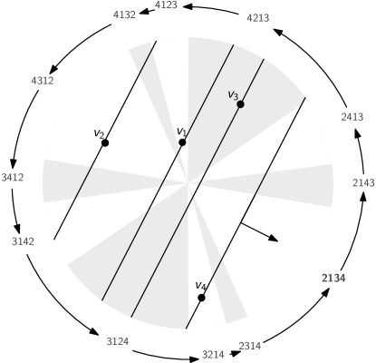
Figure 40: The allowable sequence arising from the point configuration $v_{1},v_{2},v_{3},v_{4}$. Alternating shaded and un-shaded regions correspond to cones of sweep directions which yield particular orders.

An allowable sequence is realizable if it arises from a planar point configuration. As with oriented matroids, not every allowable sequence is realizable, and realizablity is difficult to determine. By [98], checking whether an allowable sequence is realizable is complete for the existential theory of the reals.

Using allowable sequences to estimate underlying rank

Now, we notice the connection between monotone rank and allowable sequences. If $A$ is a matrix of monotone rank two, each column of $A$ corresponds to a sweep order a point arrangement in the plane. This means that there is a realizable allowable sequence which contains the column permutations of $A$ in some order. In order to translate notation between notation used for allowable sequences and notation used for monotone rank, we introduce the sort permutation of a list of numbers.

Definition 0.38.

Let $a=[a_{1},\ldots,a_{n}]$ be a vector with real entries. The sort permutation $\pi(a)$ of $a$ is the order of entries in $a$: that is, $\pi(a)_{i}$ lists the index of thesm $i$-th smallest entry of $a$.

Observation 0.1.

A matrix $A$ has monotone rank two if and only if the set of sort permutations of its columns can be ordered such that they form a subsequence of a realizable allowable sequence.

Because realizability is difficult to check, a weaker version of this observation is more useful.

Observation 0.2.

If a matrix $A$ has monotone rank two, then the sort permutations of its columns can be ordered such that they form a subsequence of an allowable sequence.

Notice this condition is also satisfied if a matrix has underlying rank two. We show that this condition is relatively easy to check.

Proposition 0.20.

A circular sequence of permutations $S=\pi_{1},\pi_{2},\ldots,\pi_{2m}$ such that $\pi\in S\Leftrightarrow-\pi\in S$ is a subsequence of an allowable sequence if and only if satisfies condition (3) to be an allowable sequence: the order of each pair $i,j$ is reversed exactly once between each $\pi_{k},-\pi_{k}=\pi_{k+m}$

Proof.

To prove the “only if" part of this proposition, we note that if we fail to meet condition (3), we cannot fix it by adding more permutations. To prove the other direction, we construct a simple allowable sequence $\sigma_{1},\ldots,\sigma_{2M}$ containing $\pi_{1},\pi_{2},\ldots,\pi_{2m}$ as a subsequence. We need to show that for each $\pi_{i},\pi_{i+1}$, we can fill in

$$\pi_{i}=\sigma_{j},\sigma_{j+1},\ldots,\sigma_{j+k}=\pi_{i+1}$$

such that each ${\sigma_{j}},\sigma_{j+1}$ differs by reversing a pair of adjacent entries.

We are able to do this iteratively for each pair: to produce $\sigma_{j+1}$ from $\sigma_{j}$, we look for a pair of adjacent elements of $\sigma_{j}$ which are in the reverse order of their order in $\pi_{i+1}.$ We reverse this pair to produce $\sigma_{j+1}$ from $\sigma_{j}.$ Once there is nothing left to reverse, we have arrived at $\pi_{i+1}$.

We do this for each pair $\pi_{i},\pi_{i+1}$ until we reach $\sigma_{k}=-\pi_{i}$. From here, we fill in the rest of the allowable sequence using the rule $\sigma_{i+k}=-\sigma_{i}$. By construction, we have clearly satisfied conditions (1) and (2) to be an allowable sequence. Now, notice that since we only reverse a pair of elements between $\sigma_{j},\sigma_{j+1}$ if $i$ and $j$ were reversed between some $\pi_{i}$ and $\pi_{i+1}$, we do not introduce any extra swaps of each pair between any $\pi_{i}$, $-\pi_{i}$. Thus, each pair $i,j$ is reversed exactly once between each $\sigma_{i},-\sigma_{i}=\sigma_{i+k}$. Thus, $\sigma_{1},\sigma_{2},\ldots,\sigma_{2k}$ is an allowable sequence. ∎

Example 0.10.

The matrix

$$A=\begin{pmatrix}1&2&1&1\\ 2&1&3&2\\ 3&3&2&4\\ 4&4&4&3\end{pmatrix}$$

has Radon rank two and monotone rank three. To see that the Radon rank is two, note that no column of the matrix induces the partition $(14,23)$. To see that the monotone rank is three, we consider its set of column permutations and reversed column permutations

$$1234,2134,1324,1243,4321,4312,4213,3412$$

By brute force, we can see that there is no ordering which satisfies Proposition 0.20. Thus, by Observation 0.2,

$$\operatorname{urank}(A)\geq\operatorname{mrank}(A)\geq 3.$$

We will later show how to determine this much more efficiently.

Next, we give an $O(mn^{2})$ algorithm to determine whether the column permutations of a matrix can be placed in an order which satisfies the conditions of Proposition 0.20. This algorithm makes use of a definition of distance between two permutations.

Definition 0.39.

Given two permutations $\pi,\sigma$, define their distance by

$$d(\pi,\sigma)=|\{\{i,j\}\mid i\mbox{ and }j\mbox{ are swapped between }\pi\mbox{ and }\sigma\}|.$$

Lemma 0.7.

Let $\pi_{i},\pi_{j},\pi_{k}$ be permutations of $[n]$. Then $\pi_{j}$ is allowed between $\pi_{i}$ and $\pi_{k}$ if and only if $d(\pi_{i},\pi_{j})+d(\pi_{j},\pi_{k})=d(\pi_{i},\pi_{k})$.

Algorithm
Input: A sequence of permutations $\pi_{1},\ldots,\pi_{2n}$
Output: The same sequence of permutations, sorted in an order which satisfies Proposition 0.20, if possible. Otherwise, the algorithm will report failure.

Step one: For each $j\geq 1$ compute and record $d(\pi_{i},\pi_{j})$. Sort the permutations in the order of increasing $d(\pi_{i},\pi_{j})$, resolving ties arbitrarily. From here on out, we will assume that $\pi_{1},\ldots,\pi_{n}$ is written in this order.
Step two: Now, we begin placing the permutations into a new order satisfying Proposition 0.20. We first construct only the first half of this order, between $\pi_{1}$ and $-\pi_{1}$, placing $\pi_{1}$ at the first spot in this order and $-\pi_{1}$ at the last spot. Now, beginning with $\pi_{2}$ and continuing in our sorted order until we reach $\pi_{2n}$, we check whether each new entry to be added $\pi_{i}$ is allowed between the last permutation added to the list, $\pi_{j}$, and $-\pi_{1}.$ If yes, we insert it there. If not, we do not.
Step three: Now, we check whether, for each pair $\pi_{i},-\pi_{i}$, we have inserted at least one member of the pair into the sequence. If we have not, we report failure. If we have, we then complete the rest of the sequence using the rule $\pi_{i+n}=-\pi_{i}$. We return this sequence.

Example 0.11.

We apply our algorithm to the matrix

$$A=\begin{pmatrix}1&2&1&1\\ 2&1&3&2\\ 3&3&2&4\\ 4&4&4&3\end{pmatrix}$$

from Example 0.10, trying to fit the set of column permutations and their reverses

$$1234,2134,1324,1243,4321,4312,4231,3421$$

into a sequence satisfying Proposition 0.20.
Step one: Sorting by distance from $1234$, we have

$$1234,2134,1324,1243,4312,4231,3421,4321$$

Step two: Now, we begin a new sequence with

$$1234,4321$$

• Now, we check whether $2134$ is allowed between $1234$ and $4321$. It is, so we insert it

  $$1234,2134,4321$$

• Next, we check whether $1324$ is allowed between $2134$ and $4321$. It is not, because the pair $12$ gets reversed twice along the sequence.

• Next, we check whether $1243$ is allowed between $2134$ and $4321$. Again, it is not, because the pair $12$ gets reversed twice along the sequence.

• Next, we check whether $4312$ is allowed between $2134$ and $4321$. Again, it is not, because the pair $12$ gets reversed twice along the sequence.

• Next, we check whether $4231$ is allowed between $2134$ and $4321$. It is, so we insert it

  $$1234,2134,4231,4321$$

• Finally, we check whether $3421$ is allowed between $4231$ and $4321.$ It is not, because the pair $34$ is reversed twice along the sequence.

Thus, the final sequence we have constructed is

$$1234,2134,4231,4321$$

Step three We report failure because we have not inserted either member of the pair $1243,3412$.

Proposition 0.21.

The sequence of permutations returned by this algorithm is a subsequence of an allowable sequence. If the algorithm reports failure, then these is no way to reorder $\pi_{1},\cdots,\pi_{n}$ so that they form a subsequence of an allowable sequence. The worst case runtime of this algorithm is $O(mn^{2})$.

Proof.

We first prove that any sequence of permutations returned by this algorithm is a subsequence of an allowable sequence using Proposition 0.20. By construction, we have that $\pi\in S\Leftrightarrow-\pi\in S$. Now, we check that each pair of points is reversed exactly along the sequence between $\pi_{1}$ and $-\pi_{1}$. Note that this property is present at the beginning of Step 2, when the sequence is $\pi_{1},\pi_{2},-\pi_{1}$. Now, we show that it is maintained every time we insert a permutation. Every time we insert a permutation $\pi_{i}$ between $\pi_{j}$ and $-\pi_{1}$, we check whether $\pi_{i}$ is allowed between $\pi_{j}$ and $-\pi_{1}$. This means that if a pair of points is reversed between $\pi_{1}$ and $\pi_{j}$, then it is not reversed again between $\pi_{j}$ and $\pi_{i}$. Thus, we satisfy condition (3) as well.

Now, we prove that if the algorithm reports failure, then there is no allowable sequence containing all of the permutations. Suppose there exists such an allowable sequence. Without loss of generality, we can assume that the permutation $\pi_{2}$ comes after $\pi_{1}$ and before $-\pi_{1}$ in this sequence, since otherwise we can reverse the order of the sequence to get another allowable sequence. Now, notice that as we move along the sequence from $\pi_{1}$ to $\pi_{n}$, the distance of each permutation from $\pi_{1}$ must increase monotonically. Thus, a permutation $\pi_{j}$ must be inserted into the sequence at the position chosen by the algorithm if it can be inserted into the sequence at all. Further, since every pair is reversed between permutations $\pi_{i}$ and $-\pi_{i}$, for all $i\neq 1$, exactly one of $\pi_{i}$ and $-\pi_{i}$ appears between $\pi_{1}$ and $-\pi_{1}$ in a sequence. Thus, if we apply this algorithm to a set of permutations which can be arranged to form a subsequence of an allowable sequence, for each $i$, we can fit either $\pi_{i}$ or $-\pi_{i}$ into the sequence, so we do not report failure.

Finally, we prove that the running time is $O(mn^{2})$ for a set of $m$ sequences of $n$ points. In step one, we can compute the distance between two permutations in time $O(n^{2})$. Thus, we can compute all of the distances from $\pi_{1}$ to $\pi_{i}$ in time $O(mn^{2})$. Next, we can sort the sequences by distance in time $O(m\log m).$ Asymptotically, we must have $\log m<n^{2}$, thus the overall runtime scales as $O(mn^{s})$. In step two, we look at each permutation $\pi_{j}$ once and compute two distances $d(\pi_{i},\pi_{j})$ and $d(\pi_{j},-\pi_{1})$ to determine whether $\pi_{j}$ can be placed into the sequence. Thus, we can do step two in time $O(mn^{2})$ as well. Finally, we check whether for each $\pi_{i}$, we have placed either $\pi_{i}$ or $-\pi_{i}$ into the sequence in time $O(n)$, since the fact that the list is sorted by distance from $\pi_{1}$ means that we know where to look for $-\pi_{i}$ given $\pi_{i}$.

∎

Computing underlying rank is hard

Now, we apply the result of [98] that the problem of checking realizability for allowable sequences is complete in the existential theory of the reals $(\exists\mathbb{R})$ in order to prove that determining whether a matrix has monotone rank two is $\exists\mathbb{R}$-complete. We then apply this result to show that determining whether a matrix has underlying rank two is $\exists\mathbb{R}$-complete as well.

Proposition 0.22.

Checking whether a matrix has monotone rank two is complete $\exists\mathbb{R}$-complete and therefore NP-hard.

Proof.

We can reduce the problem of determining whether an allowable sequence is realizable to the problem of determining whether a matrix has monotone rank two. Given an allowable sequence $\pi_{1},\ldots,\pi_{m}$, we can construct a matrix $A$ whose columns have sort permutations $\pi_{1},\ldots,\pi_{m}$. By Observation 0.2, $A$ has monotone rank two if and only if $\pi_{1},\ldots,\pi_{m}$ form a subsequence of a realizable allowable sequence. ∎

Thus, we have shown that the problem of computing monotone rank is computationally intractable.

Finally, we show that computing underlying rank is intractable. We do this by reducing the problem of determining whether an allowable sequence is realizable to the problem of determining whether a matrix has underlying rank two.

To to this, we construct a matrix $A(\pi_{1},\ldots,\pi_{2n})$ which has rank two if and only if $\pi_{1},\ldots,\pi_{2n}$ is realizable. Ensure that the $i^{th}$ column of $A$ has the sort permutation $\pi_{i}$. Now, scale each column that $A_{ij}>A_{k\ell}$ whenever $j>\ell$. We prove the following:

Lemma 0.8.

The matrix $A(\pi_{1},\ldots,\pi_{2n})$ has underlying rank two if and only if $\pi_{1},\ldots,\pi_{2n}$ is realizable.

Proof.

First, notice that if $A$ has underlying rank two, then it also has monotone rank two. Thus by Observation 0.2, $\pi_{1},\ldots,\pi_{2n}$ is realizable.

Now, suppose $\pi_{1},\ldots,\pi_{2n}$ is realizable by the point configuration $v_{1},\ldots,v_{m}$. Let $i,j$ be the pair of indices whose order is switched between $\pi_{2n}$ and $\pi_{1}$. Let $x_{ij}$ be the vector which points from $v_{i}$ to $v_{j}$. We produce a new point configuration $v_{1},\ldots,v_{m}$ by letting $v^{\prime}_{k}=v_{k}+Cx_{ij}$ for some constant $C$. We can chose the constant $C$ and sweep vectors $w_{1},\ldots,w_{m}$ such that the matrix $B_{ij}=w_{i}v_{j}$ is a rank two realization of $A$.

Notice that for any $\epsilon>0$, we can choose a value of $C$ such that the angle between the vectors $v_{k}^{\prime}$ and $v_{j}^{\prime}-v_{i}^{\prime}=v_{j}-v_{i}$ is less than $\epsilon.$ Thus, we choose $C$ such that the angle between $v_{j}^{\prime}-v_{i}^{\prime}$ and $v_{k}^{\prime}$ is smaller than the angle between $v_{j}^{\prime}-v_{i}^{\prime}$ and any $v_{\ell}^{\prime}-v_{p}^{\prime}$.

Thus when we cyclically order the vectors $\{v_{k}^{\prime}\}_{k\in[m]}\cup\{v_{k}^{\prime}-v_{\ell}^{\prime}\}_{k,\ell\in[m]}$, all of the vectors $v_{k}^{\prime}$ are closer to $v_{j}-v_{i}$ then they are to any other $v_{k}^{\prime}-v_{\ell}^{\prime}$. This means that when we consider the allowable sequence of the larger point arrangement $\{v_{k}^{\prime}\}_{k\in[m]}\cup\{\mathbf{0}\}$, each permutation which has $i$ before $j$ occurs with $\mathbf{0}$ at the beginning, and each permutation with $j$ before $i$ occurs with $\mathbf{0}$ at the end.

Thus for each permutation $\pi_{k}$ in the allowable sequence, we can choose a sweep direction $w_{k}$ which sweeps past $v_{1},\ldots,v_{m}$ in the order $\pi_{k}$, with $v_{\ell}\cdot w_{k}>0$ for all permutations with $i$ before $j$ and $v_{\ell}\cdot w_{k}<0$ for all permutations with $j$ before $i$. Now, we rescale each $w_{k}$ to get a new vector $w_{k}^{\prime}$ so as to satisfy the condition that $A_{ij}>A_{k\ell}$ whenever $j>\ell$. For the first $n$ permutations, $i$ comes before $j$, so $v_{\ell}\cdot w_{k}^{\prime}>0$. As we increase $k$ we can shrink the magnitude of $w_{k}^{\prime}$ to satisfy $v_{i}^{\prime}\cdot w_{j}^{\prime}\leq v_{k}^{\prime}w_{k+1}^{\prime}$. Once we pass permutation $\pi_{n+1}$, $j$ comes before $i$, and so the inner products satisfy $v_{\ell}\cdot w_{k}<0$. Now, as we increase $k$, we can increase the magnitude of $w_{k}^{\prime}$ as we increase $k$ in order to satisfy $v_{i}^{\prime}\cdot w_{j}^{\prime}\leq v_{k}^{\prime}w_{k+1}^{\prime}$.

Thus, $v_{1},\ldots,v_{m},w_{1},\ldots,w_{2n}$ is a rank two representation of $A$.

∎

Theorem 0.3.

Checking whether a matrix has underlying rank two is $\exists\mathbb{R}$-complete and thus NP-hard.

Proof.

We show that there is a reduction from the problem of determining whether an allowable sequence is realizable to the problem of determining whether a matrix has underlying rank two. Let $\pi_{1},\ldots,\pi_{2n}$ be an allowable sequence. Then by Lemma 0.8, the matrix $A(\pi_{1},\ldots,\pi_{2n})$ has underlying rank two if and only if $\pi_{1},\ldots,\pi_{2n}$ is realizable. Thus, there is a polynomial time reduction from the problem of determining whether an allowable sequence is representable to the problem of determining whether a matrix has underlying rank two. Thus, checking whether a matrix has underlying rank two is $\exists\mathbb{R}$-complete and thus NP-hard. ∎

Conclusion and Open Questions

In this chapter, we introduced the concept of the underlying rank of a matrix, and introduced a set of techniques for estimating it. Many open questions, of both biological and mathematical interest, remain. We highlight some here.

In Section Radon’s theorem: a lower bound for underlying rank, we introduce the Radon rank of a matrix as a lower bound for its underlying rank. However, the Radon rank is not stable under localized noise: shattering even one set of size $d+1$ is enough to raise the Radon rank to $d$, while only involving $d+1$ rows of the matrix.

In Section The combinatorial geometry of underlying rank, we use the theory of oriented matroids and allowable sequences to give lower bounds on underlying rank. Our work in this section leaves open interesting questions in oriented matroid theory. In particular, our Theorem 0.2 states that if a matrix has underlying rank $d$ if its potential circuits of rank $d$ contain the circuits of an oriented matroid of rank $d+1$. This serves as a “combinatorial relaxation" of the underlying rank problem. While computing the underlying rank problem is not computationally tractable, this relaxed version may be.

Question 0.17.

Is there a combinatorial characterization of the when a given set of potential circuits contain the circuits of an oriented matroid? Is there an efficient algorithm to determine whether this is the case?

These questions suggest building a more general theory of “partial oriented matroids" which asks when a given set of sign vectors can be extended to be the set of topes or circuits of an oriented matroid. Progress in this area would also be helpful towards answering Question 0.8, since knowing an oriented matroid lives above a certain code also provides partial information about the matroid.

Threshold-Linear Networks

SupplementaryMaterial/Vita

References

- [1] O’Keefe, J. (1976) “Place units in the hippocampus of the freely moving rat,” Experimental neurology, 51(1), pp. 78–109.
- [2] Curto, C., V. Itskov, A. Veliz-Cuba, and N. Youngs (2013) “The neural ring: an algebraic tool for analyzing the intrinsic structure of neural codes,” Bulletin of mathematical biology, 75(9), pp. 1571–1611.
- [3] Curto, C. (2017) “What can topology tell us about the neural code?” Bulletin of the American Mathematical Society, 54(1), pp. 63–78.
- [4] Curto, C., E. Gross, J. Jeffries, K. Morrison, M. Omar, Z. Rosen, A. Shiu, and N. Youngs (2017) “What makes a neural code convex?” SIAM Journal on Applied Algebra and Geometry, 1(1), pp. 222–238.
- [5] Franke, M. K. and S. Muthiah (2017) “Every neural code can be realized by convex sets,” Preprint.
- [6] Cruz, J., C. Giusti, V. Itskov, and B. Kronholm (2019) “On open and closed convex codes,” Discrete & computational geometry, 61(2), pp. 247–270.
- [7] Chen, A., F. Frick, and A. Shiu (2019) “Neural codes, decidability, and a new local obstruction to convexity,” SIAM Journal on Applied Algebra and Geometry, 3(1), pp. 44–66.
- [8] Lienkaemper, C., A. Shiu, and Z. Woodstock (2017) “Obstructions to convexity in neural codes,” Advances in Applied Mathematics, 85, pp. 31–59.
- [9] Jeffs, R. A. (2019) “Sunflowers of convex open sets,” Advances in Applied Mathematics, 111, p. 101935.
- [10] ——— (2020) “Morphisms of neural codes,” SIAM Journal on Applied Algebra and Geometry, 4(1), pp. 99–122.
- [11] Kunin, A., C. Lienkaemper, and Z. Rosen (2020) “Oriented matroids and combinatorial neural codes,” arXiv preprint arXiv:2002.03542.
- [12] Itskov, V., A. Kunin, and Z. Rosen (2020) “Hyperplane neural codes and the polar complex,” in Topological Data Analysis, Springer, pp. 343–369.
- [13] Gambacini, B., R. A. Jeffs, S. Macdonald, and A. Shiu (2021) “Non-monotonicity of closed convexity in neural codes,” Vietnam Journal of Mathematics, pp. 1–15.
- [14] Chan, P., K. Johnston, J. Lent, A. R. de Perez, and A. Shiu (2020) “Nondegenerate neural codes and obstructions to closed-convexity,” arXiv preprint arXiv:2011.04565.
- [15] Jeffs, R. A. (2021) “Open, closed, and non-degenerate embedding dimensions of neural codes,” arXiv preprint arXiv:2111.01010.
- [16] ——— (2022) “Embedding dimension phenomena in intersection complete codes,” Selecta Mathematica, 28(1), pp. 1–37.
- [17] Jeffs, R. A. and I. Novik (2021) “Convex union representability and convex codes,” International Mathematics Research Notices, 2021(9), pp. 7132–7158.
- [18] Goldrup, S. A. and K. Phillipson (2020) “Classification of open and closed convex codes on five neurons,” Advances in Applied Mathematics, 112, p. 101948.
- [19] Johnston, K., A. Shiu, and C. Spinner (2020) “Neural codes with three maximal codewords: Convexity and minimal embedding dimension,” arXiv preprint arXiv:2008.13192.
- [20] Kalai, G. (1984) “Characterization of f-vectors of families of convex sets inR d Part I: Necessity of Eckhoff’s conditions,” Israel Journal of Mathematics, 48(2), pp. 175–195.
- [21] ——— (1986) “Characterization of f-vectors of families of convex sets in Rd part II: Sufficiency of Eckhoff’s conditions,” Journal of Combinatorial Theory, Series A, 41(2), pp. 167–188.
- [22] Matoušek, J. and M. Tancer (2009) “Dimension gaps between representability and collapsibility,” Discrete & Computational Geometry, 42(4), pp. 631–639.
- [23] Tancer, M. (2013) “Intersection patterns of convex sets via simplicial complexes: a survey,” in Thirty essays on geometric graph theory, Springer, pp. 521–540.
- [24] Sturmfels, B. (1987) “On the decidability of Diophantine problems in combinatorial geometry,” Bulletin (New series) of the American Mathematical Society, 17(1), pp. 121–124.
- [25] Mnëv, N. E. (1988) “The universality theorems on the classification problem of configuration varieties and convex polytopes varieties,” in Topology and geometry—Rohlin seminar, Springer, pp. 527–543.
- [26] Shor, P. (1991) “Stretchability of pseudolines is NP-hard,” Applied Geometry and Discrete Mathematics-The Victor Klee Festschrift.
- [27] Jeffs, R. A., C. Lienkaemper, and N. Youngs (2020) “Order-forcing in neural codes,” arXiv preprint arXiv:2011.03572.
- [28] Gao, P. and S. Ganguli (2015) “On simplicity and complexity in the brave new world of large-scale neuroscience,” Current opinion in neurobiology, 32, pp. 148–155.
- [29] Cowley, B. R., M. A. Smith, A. Kohn, and B. M. Yu (2016) “Stimulus-driven population activity patterns in macaque primary visual cortex,” PLoS computational biology, 12(12), p. e1005185.
- [30] Pang, R., B. J. Lansdell, and A. L. Fairhall (2016) “Dimensionality reduction in neuroscience,” Current Biology, 26(14), pp. R656–R660.
- [31] Chaudhuri, R., B. Gercek, B. Pandey, A. Peyrache, and I. Fiete (2019) “The intrinsic attractor manifold and population dynamics of a canonical cognitive circuit across waking and sleep,” Nature neuroscience, 22(9), pp. 1512–1520.
- [32] Zhou, Y., B. H. Smith, and T. O. Sharpee (2018) “Hyperbolic geometry of the olfactory space,” Science advances, 4(8), p. eaaq1458.
- [33] Fusi, S., E. K. Miller, and M. Rigotti (2016) “Why neurons mix: high dimensionality for higher cognition,” Current opinion in neurobiology, 37, pp. 66–74.
- [34] Farrell, M., S. Recanatesi, G. Lajoie, and E. Shea-Brown (2019) “Dynamic compression and expansion in a classifying recurrent network,” bioRxiv, p. 564476.
- [35] Akerboom, J., T.-W. Chen, T. J. Wardill, L. Tian, J. S. Marvin, S. Mutlu, N. C. Calderón, F. Esposti, B. G. Borghuis, X. R. Sun, et al. (2012) “Optimization of a GCaMP calcium indicator for neural activity imaging,” Journal of neuroscience, 32(40), pp. 13819–13840.
- [36] Nauhaus, I., K. J. Nielsen, and E. M. Callaway (2012) “Nonlinearity of two-photon Ca2+ imaging yields distorted measurements of tuning for V1 neuronal populations,” Journal of Neurophysiology, 107(3), pp. 923–936.
- [37] Giusti, C., E. Pastalkova, C. Curto, and V. Itskov (2015) “Clique topology reveals intrinsic geometric structure in neural correlations,” Proceedings of the National Academy of Sciences, 112(44), pp. 13455–13460.
- [38] Curto, C., J. Paik, and I. Rivin (2021) “Betti Curves of Rank One Symmetric Matrices,” arXiv preprint arXiv:2103.00761.
- [39] Goodman, J. E. and R. Pollack (1991) “The complexity of point configurations,” Discrete Applied Mathematics, 31(2), pp. 167–180.
- [40] Björner, A., M. Las Vergnas, B. Sturmfels, N. White, and G. M. Ziegler (1999) Oriented matroids, 46, Cambridge University Press.
- [41] Hahnloser, R. and H. S. Seung (2000) “Permitted and forbidden sets in symmetric threshold-linear networks,” Advances in neural information processing systems, 13.
- [42] Borsuk, K. (1948) “On the imbedding of systems of compacta in simplicial complexes,” Fundamenta Mathematicae, 35(1), pp. 217–234.
- [43] Leray, J. (1950) “L’anneau spectral et l’anneau filtré d’homologie d’un espace localement compact et d’une application continue,” J. Math. Pures Appl, 29(9), pp. 1–139.
- [44] Weil, A. (1952) “Sur les théorèmes de de Rham,” Commentarii Mathematici Helvetici, 26(1), pp. 119–145.
- [45] Hatcher, A. (2001) Algebraic topology, Cambridge University Press;.
- [46] Helly, E. (1923) “Über Mengen konvexer Körper mit gemeinschaftlichen Punkte.” Jahresbericht der Deutschen Mathematiker-Vereinigung, 32, pp. 175–176.
- [47] Kalai, G. (1984) “Intersection patterns of convex sets,” Israel Journal of Mathematics, 48(2), pp. 161–174.
- [48] Wegner, G. (1975) “d-Collapsing and nerves of families of convex sets,” Archiv der Mathematik, 26(1), pp. 317–321.
- [49] Tancer, M. (2010) “d-collapsibility is NP-complete for d greater than or equal to 4,” Chicago Journal of Theoretical Computer Science.
- [50] ——— (2010) “A counterexample to Wegner’s conjecture on good covers,” arXiv preprint arXiv:1008.1895.
- [51] Radon, J. (1921) “Mengen konvexer Körper, die einen gemeinsamen Punkt enthalten,” Mathematische Annalen, 83(1), pp. 113–115.
- [52] Folkman, J. and J. Lawrence (1978) “Oriented matroids,” Journal of Combinatorial Theory, Series B, 25(2), pp. 199–236.
- [53] Broglia, F. (1996) Lectures in real geometry, de Gruyter.
- [54] Schaefer, M. (2009) “Complexity of some geometric and topological problems,” in International Symposium on Graph Drawing, Springer, pp. 334–344.
- [55] Vámos, P. (1978) “The missing axiom of matroid theory is lost forever,” Journal of the London Mathematical Society, 2(3), pp. 403–408.
- [56] Mayhew, D., G. Whittle, and M. Newman (2014) “Is the missing axiom of matroid theory lost forever?” Quarterly Journal of Mathematics, 65(4), pp. 1397–1415.
- [57] Mayhew, D., M. Newman, and G. Whittle (2018) “Yes, the “missing axiom” of matroid theory is lost forever,” Transactions of the American Mathematical Society, 370(8), pp. 5907–5929.
- [58] Tolman, E. C. (1948) “Cognitive maps in rats and men.” Psychological review, 55(4), p. 189.
- [59] O’Keefe, J. and J. Dostrovsky (1971) “The hippocampus as a spatial map: Preliminary evidence from unit activity in the freely-moving rat.” Brain research.
- [60] Knierim, J. J., H. S. Kudrimoti, and B. L. McNaughton (1995) “Place cells, head direction cells, and the learning of landmark stability,” Journal of Neuroscience, 15(3), pp. 1648–1659.
- [61] Yim, M. Y., L. A. Sadun, I. R. Fiete, and T. Taillefumier (2021) “Place-cell capacity and volatility with grid-like inputs,” Elife, 10, p. e62702.
- [62] Brown, E. N., L. M. Frank, D. Tang, M. C. Quirk, and M. A. Wilson (1998) “A statistical paradigm for neural spike train decoding applied to position prediction from ensemble firing patterns of rat hippocampal place cells,” Journal of Neuroscience, 18(18), pp. 7411–7425.
- [63] Curto, C. and V. Itskov (2008) “Cell groups reveal structure of stimulus space,” PLoS computational biology, 4(10), p. e1000205.
- [64] Giusti, C. and V. Itskov (2014) “A no-go theorem for one-layer feedforward networks,” Neural computation, 26(11), pp. 2527–2540.
- [65] Edelman, P. H., V. Reiner, and V. Welker (2002) “Convex, acyclic, and free sets of an oriented matroid,” Discrete & Computational Geometry, 27(1), pp. 99–116.
- [66] Tancer, M. and D. Tonkonog (2013) “Nerves of good covers are algorithmically unrecognizable,” SIAM Journal on Computing, 42(4), pp. 1697–1719.
- [67] Curto, C., C. Lienkaemper, J. L. Alvarez, and H. R. S. Cruz “A novel notion of rank for neural data analysis,” In preparation.
- [68] Huang, L., P. Ledochowitsch, U. Knoblich, J. Lecoq, G. J. Murphy, R. C. Reid, S. E. de Vries, C. Koch, H. Zeng, M. A. Buice, et al. (2021) “Relationship between simultaneously recorded spiking activity and fluorescence signal in GCaMP6 transgenic mice,” Elife, 10, p. 51675.
- [69] Siegle, J. H., P. Ledochowitsch, X. Jia, D. J. Millman, G. K. Ocker, S. Caldejon, L. Casal, A. Cho, D. J. Denman, S. Durand, et al. (2021) “Reconciling functional differences in populations of neurons recorded with two-photon imaging and electrophysiology,” Elife, 10, p. 69068.
- [70] Hansel, D. and C. Van Vreeswijk (2002) “How noise contributes to contrast invariance of orientation tuning in cat visual cortex,” Journal of Neuroscience, 22(12), pp. 5118–5128.
- [71] Dunn, J. C. and L. Anderson (2018) “Signed difference analysis: Testing for structure under monotonicity,” Journal of Mathematical Psychology, 85, pp. 36–54.
- [72] Dunn, J. C. and R. N. James (2003) “Signed difference analysis: Theory and application,” Journal of Mathematical Psychology, 47(4), pp. 389–416.
- [73] Weinreich, D. M., N. F. Delaney, M. A. DePristo, and D. L. Hartl (2006) “Darwinian evolution can follow only very few mutational paths to fitter proteins,” science, 312(5770), pp. 111–114.
-
[74]
Husain, K. and A. Murugan (2020) “Physical
Constraints on Epistasis,” Molecular Biology and Evolution, cvaa128,
https://academic.oup.com/mbe/advance-article-pdf/doi/10.1093/molbev/msaa124/33427979/msaa124.pdf.
URL https://doi.org/10.1093/molbev/msaa124 - [75] Otwinowski, J. (2018) “Biophysical inference of epistasis and the effects of mutations on protein stability and function,” Molecular biology and evolution, 35(10), pp. 2345–2354.
- [76] Cunningham, J. P. and M. Y. Byron (2014) “Dimensionality reduction for large-scale neural recordings,” Nature neuroscience, 17(11), pp. 1500–1509.
- [77] Stringer, C., M. Pachitariu, N. Steinmetz, M. Carandini, and K. D. Harris (2019) “High-dimensional geometry of population responses in visual cortex,” Nature, 571(7765), pp. 361–365.
- [78] Machens, C. K., R. Romo, and C. D. Brody (2010) “Functional, but not anatomical, separation of “what” and “when” in prefrontal cortex,” Journal of Neuroscience, 30(1), pp. 350–360.
- [79] Chapin, J. K. and M. A. Nicolelis (1999) “Principal component analysis of neuronal ensemble activity reveals multidimensional somatosensory representations,” Journal of neuroscience methods, 94(1), pp. 121–140.
- [80] Churchland, M. M., J. P. Cunningham, M. T. Kaufman, J. D. Foster, P. Nuyujukian, S. I. Ryu, and K. V. Shenoy (2012) “Neural population dynamics during reaching,” Nature, 487(7405), pp. 51–56.
- [81] Ding, J. and A. Zhou (2007) “Eigenvalues of rank-one updated matrices with some applications,” Applied Mathematics Letters, 20(12), pp. 1223–1226.
- [82] Barany, I. and C. Buchta (1993) “Random polytopes in a convex polytope, independence of shape, and concentration of vertices,” Mathematische Annalen, 297(1), pp. 467–497.
- [83] Baryshnikov, Y. M. and R. A. Vitale (1994) “Regular simplices and Gaussian samples,” Discrete & Computational Geometry, 11(2), pp. 141–147.
- [84] Raynaud, H. (1970) “Sur l’enveloppe convexe des nuages de points aléatoires dans Rn. I,” Journal of Applied Probability, 7(1), pp. 35–48.
- [85] De Silva, V. and G. E. Carlsson (2004) “Topological estimation using witness complexes.” SPBG, 4, pp. 157–166.
- [86] Vapnik, V. N. and A. Y. Chervonenkis (1971) “On the Uniform Convergence of Relative Frequencies of Events to Their Probabilities,” Theory of Probability & Its Applications, 16(2), p. 264?280.
- [87] Rigotti, M., O. Barak, M. R. Warden, X.-J. Wang, N. D. Daw, E. K. Miller, and S. Fusi (2013) “The importance of mixed selectivity in complex cognitive tasks,” Nature, 497(7451), pp. 585–590.
- [88] Dilworth, R. P. (1950) “A decomposition theorem for partially ordered sets,” in Annals of Mathematics, Mathematics Department, Princeton University, pp. 161–166.
- [89] Sperner, E. (1928) “Ein satz über untermengen einer endlichen menge,” Mathematische Zeitschrift, 27(1), pp. 544–548.
- [90] Egger, P., V. Itskov, M.-C. Wu, and A. Yarosh “Topological detection of monotone rank,” In preparation.
- [91] Anderson, L.
- [92] Padrol, A. and E. Philippe (2021) “Sweeps, polytopes, oriented matroids, and allowable graphs of permutations,” arXiv preprint arXiv:2102.06134.
- [93] Alon, N., S. Moran, and A. Yehudayoff (2014) “Sign rank, VC dimension and spectral gaps.” in Electronic Colloquium on Computational Complexity (ECCC), vol. 21, p. 10.
- [94] Forster, J. (2002) “A linear lower bound on the unbounded error probabilistic communication complexity,” Journal of Computer and System Sciences, 65(4), pp. 612–625.
- [95] Basri, R., P. F. Felzenszwalb, R. B. Girshick, D. W. Jacobs, and C. J. Klivans (2009) “Visibility constraints on features of 3D objects,” in 2009 IEEE Conference on Computer Vision and Pattern Recognition, IEEE, pp. 1231–1238.
- [96] Bhangale, A. and S. Kopparty (2015) “The complexity of computing the minimum rank of a sign pattern matrix,” arXiv preprint arXiv:1503.04486.
- [97] Wu, M.-C. and V. Itskov (2021) “A topological approach to inferring the intrinsic dimension of convex sensing data,” Journal of Applied and Computational Topology, pp. 1–50.
- [98] Hoffmann, U. and K. Merckx (2018) “A universality theorem for allowable sequences with applications,” arXiv preprint arXiv:1801.05992.
- [99] Hartline, H. K. and F. Ratliff (1957) “Inhibitory interaction of receptor units in the eye of Limulus,” The Journal of general physiology, 40(3), pp. 357–376.
- [100] Von der Malsburg, C. (1973) “Self-organization of orientation sensitive cells in the striate cortex,” Kybernetik, 14(2), pp. 85–100.
- [101] McCulloch, W. S. and W. Pitts (1943) “A logical calculus of the ideas immanent in nervous activity,” The bulletin of mathematical biophysics, 5(4), pp. 115–133.
- [102] Hopfield, J. J. (1982) “Neural networks and physical systems with emergent collective computational abilities,” Proceedings of the national academy of sciences, 79(8), pp. 2554–2558.
- [103] Miller, K. D. and F. Fumarola (2012) “Mathematical equivalence of two common forms of firing rate models of neural networks,” Neural computation, 24(1), pp. 25–31.
- [104] Beer, R. D. (2006) “Parameter space structure of continuous-time recurrent neural networks,” Neural computation, 18(12), pp. 3009–3051.
- [105] Hahnloser, R. L. (1998) “On the piecewise analysis of networks of linear threshold neurons,” Neural Networks, 11(4), pp. 691–697.
- [106] Feng, J. and K. Hadeler (1996) “Qualitative behaviour of some simple networks,” Journal of Physics A: Mathematical and General, 29(16), p. 5019.
- [107] Curto, C. and K. Morrison (2016) “Pattern completion in symmetric threshold-linear networks,” Neural computation, 28(12), pp. 2825–2852.
- [108] Moon, J. W. and L. Moser (1965) “On cliques in graphs,” Israel journal of Mathematics, 3(1), pp. 23–28.
- [109] Curto, C., J. Geneson, and K. Morrison (2019) “Fixed points of competitive threshold-linear networks,” Neural computation, 31(1), pp. 94–155.
- [110] Curto, C., C. Langdon, and K. Morrison (2020) “Combinatorial Geometry of Threshold-Linear Networks,” arXiv preprint arXiv:2008.01032.
- [111] ——— (2019) “Robust motifs of threshold-linear networks,” arXiv preprint arXiv:1902.10270.
- [112] Morrison, K., A. Degeratu, V. Itskov, and C. Curto (2016) “Diversity of emergent dynamics in competitive threshold-linear networks: a preliminary report,” arXiv preprint arXiv:1605.04463.
- [113] Bel, A., R. Cobiaga, W. Reartes, and H. G. Rotstein (2021) “Periodic solutions in threshold-linear networks and their entrainment,” SIAM Journal on Applied Dynamical Systems, 20(3), pp. 1177–1208.
- [114] Parmelee, C., S. Moore, K. Morrison, and C. Curto (2022) “Core motifs predict dynamic attractors in combinatorial threshold-linear networks,” PloS one, 17(3), p. e0264456.
- [115] Parmelee, C., J. L. Alvarez, C. Curto, and K. Morrison (2021) “Sequential attractors in combinatorial threshold-linear networks,” arXiv preprint arXiv:2107.10244.
- [116] Tang, H., K. C. Tan, and W. Zhang (2005) “Analysis of cyclic dynamics for networks of linear threshold neurons,” Neural computation, 17(1), pp. 97–114.