The Development of Spatial Attention U-Net for The Recovery of Ionospheric Measurements and The Extraction of Ionospheric Parameters
Abstract
We train a deep learning artificial neural network model, Spatial Attention U-Net to recover useful ionospheric signals from noisy ionogram data measured by Hualien’s Vertical Incidence Pulsed Ionospheric Radar. Our results show that the model can well identify F2 layer ordinary and extraordinary modes (F2o, F2x) and the combined signals of the E layer (ordinary and extraordinary modes and sporadic Es). The model is also capable of identifying some signals that were not labeled. The performance of the model can be significantly degraded by insufficient number of samples in the data set. From the recovered signals, we determine the critical frequencies of F2o and F2x and the intersection frequency between the two signals. The difference between the two critical frequencies is peaking at 0.63 MHz, with the uncertainty being 0.18 MHz.
Radio Science Department of Space Science and Engineering, National Central University, Taoyuan City 320317, Taiwan Skobeltsyn Institute of Nuclear Physics, Lomonosov Moscow State University, 119899 Moscow, Russia Department of Computer Science and Information Engineering, National Central University, Taoyuan City 320317, Taiwan Center for Space and Remote Sensing Research, National Central University, Taoyuan City 320317, Taiwan AI Research Center, Hon Hai Research Institute, Taipei 114699, Taiwan
Guan-Han Huangenter468@g.ncu.edu.tw
A deep learning model is applied to the ionogram recovery.
The model can well identify the combined signals of the sporadic E layer and the ordinary and extraordinary modes of the F2 layer signal.
Critical frequencies of the modes, and the intersection frequency between them are derived.
Plain Language Summary
A large amount of images are retrieved by a specialized instrument designed to make observations in the ionosphere. These images are contaminated by instrumental noises. In order to recover useful signals from these noises, we train a deep learning model. A dataset containing the labeled signals are used for both training and validating the model performance. The desired signals are manually labeled using a labelling software. By comparing the model predictions with the labels, the results show that the model can well-identify the elongated, overlapping, or compact signals. The model is also capable of correcting some missing and incorrect labels. The performance of the model is sensitive to the data number of the corresponding labels fed to the model during training. The recovered useful signals are then used to estimate physical quantities which are important for the study of ionospheric physics.
1 Introduction
The ionosphere is a region of ionized gases, plasmas, populating the upper atmosphere and thermosphere [Kelley (\APACyear1989)]. The ionosphere consists of layers concentrated at specific heights. Radio waves propagate through the ionospheric layers at different group velocities and, hence, split into different wave modes according to the electron density, the magnetic field, etc. An experimental ground-based technique of ionosondes has been used for a long time to investigate the vertical profile of the ionospheric ionization represented by the density of free electrons, so-called electron content (EC).
The data product of ionosonde measurements are ionograms, which exhibit signals deflected by the ionosphere at various virtual heights as a function of the sounding frequency. The virtual height of the deflection is obtained by assuming that the wave beams are propagating at the speed of light. The sounding frequency at which the virtual height rapidly increases is called the critical frequency, which also corresponds to the local maximum of the EC. In addition, the splitting in the sounding frequency between the signals of different wave modes is related to the local magnetic field. These ionogram parameters can be used for the true height analysis [Titheridge (\APACyear1988), Tsai \BOthers. (\APACyear1995)], estimating the magnetic field strength [Piggott \BBA Rawer (\APACyear1978)], and modelling the electron density higher than the deflection height by the Chapman function [X. Huang \BBA Reinisch (\APACyear2001)]. Furthermore, the stability of some ionogram interpretation algorithms [Pulinets (\APACyear1995), Hui \BOthers. (\APACyear2018)] rely on the intersection point of the ordinary mode and the extraordinary mode signals.
The ionograms from Hualien’s Vertical Incidence Pulsed Ionospheric Radar (VIPIR) are featured by small and compact signals or thin and elongated signals. These ionograms are contaminated by stripe noises appearing in many frequency bands. \citeAsnr showed that the Hualien dataset has stronger noise signals compared with the Jicarmaca dataset [Jara \BBA Olivares (\APACyear2021)].
Thousands of measurements are produced by VIPIR per day. It is hard work and time-consuming for skilled researchers to recover ionospheric signals from such immense dataset. Therefore an automated method based on fuzzy logic [Tsai \BBA Berkey (\APACyear2000)] has been applied. In recent years, there are also deep learning techniques applied to the ionogram recovery [Mochalov \BBA Mochalova (\APACyear2019), Xiao \BOthers. (\APACyear2020), Jara \BBA Olivares (\APACyear2021)].
In this research, we implement a deep learning model to the Hualien VIPIR ionograms, and recover different ionogram signals. The data and the preprocessing of the dataset are presented in Section 2. The deep learning model and the validation of the model are described in Section 3. In Section 4, we evaluate the performance of signal recovery (in 4.1), and derive the ionogram parameters from the recovered ionograms (in 4.2). The results are discussed in Section 5 and summarized in Section 6.
2 Data
We use the ionograms acquired from the Hualien VIPIR digisonde operated at Hualien, Taiwan (N, E). The dataset contains ionograms spanning from 2013/11/08 to 2014/06/29. Each ionogram covers a virtual height range up to 800km, and sounding frequency range from 1MHz to 22MHz, and the signal amplitude range up to 100 decibels (dB).
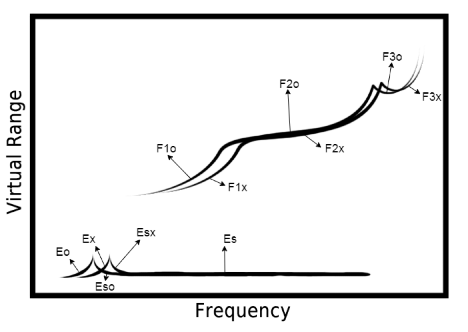
To reduce the data size and remove the calibration signals, we reduce the size of ionograms to virtual height range from 66 to 600km, and sounding frequency from 1.58 to 20.25MHz. Different useful signals in each ionogram are manually identified and labeled into polygons using labelme [Wada (\APACyear2016)]. The polygons are rasterized into a binary array of dimension 800x1600x11, which correspond, respectively, to frequency, height and the label. The eleven labels of useful signals are defined as follows (see Figure 1):
-
1.
Eo: Ordinary signal of the E-layer, with the virtual height increasing as the sounding frequency increased.
-
2.
Ex: Extra-ordinary signal of the E-layer, with the virtual height increasing as the sounding frequency increased.
-
3.
Eso: Ordinary signal of the sporadic E-layer, with the virtual height decreasing as the sounding frequency increased.
-
4.
Esx: Extra-ordinary signal of the sporadic E-layer, with the virtual height decreasing as the sounding frequency increased.
-
5.
Es: Signal of the sporadic E-layer, with the virtual height constant as the sounding frequency increased.
-
6.
F1o: Ordinary signal of the F1-layer, with the virtual height increasing as the sounding frequency increased.
-
7.
F1x: Extra-ordinary signal of the F1-layer, with the virtual height increasing as the sounding frequency increased.
-
8.
F2o: Ordinary signal of the F2-layer.
-
9.
F2x: Extra-ordinary signal of the F2-layer.
-
10.
F3o: Ordinary signal of the F3-layer, with the virtual height increasing as the sounding frequency increased.
-
11.
F3x: Extra-ordinary signal of the F3-layer, with the virtual height increasing as the sounding frequency increased.
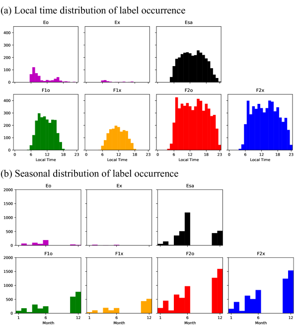
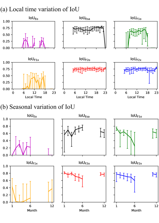
The signals shown in Figure 1 usually do not appear simultaneously in all ionograms, and some signals can be too faint to be labeled. The percentages of different labeled signals in our data set are 7.89% for Eo, 0.99% for Ex, 39.81% for Es, 13.34% for Eso, 10.59% for Esx, 39.19% for F1o, 26.06% for F1x, 94.65% for F2o, 88.90% for F2x, 0.13% for F3o and 0.16% for F3x. Eso, Esx, F3o, and F3x have very poor statistics. Therefore, we discarded F3o and F3x to increase the statistics of E layer, and combine Eso, Esx, and Es labels into the Esa label. As a result, we reduce labels into labels. The panels in Figure 2a show the local time distribution of the occurrence of the labels in the bulge of the equatorial ionoization anomaly at Taiwan. During the studied time in Taiwan, Esa, F2o, and F2x labels have the highest occurrence rate, and Eo and Ex the lowest. Sporadic Esa and F2 (F2o and F2x) layers occur at all dayside local time hours. F1 layer (F1o and F1x) does not occur in the evening. The E layer (Eo and Ex) occurs mainly in the morning. The panels in Figure 2b show the seasonal distribution of the occurrence of the layers. F2o and F2x as well as F1o and F1x appear in all seasons and have similar distributions. The sporadic layer Esa has the highest occurrence rate during the summer [Shinagawa \BOthers. (\APACyear2021)]. Our focus is to recover the Esa, F2o, and F2x labels since the radio wave propagation in the Taiwan region is mostly affected by these layers, due to their high occurrence rate.
Finally, the dataset was split into ratios of 64%, 16% and 20%, respectively, for the training set, the validation set and the test set, resulting in 3925, 981, 1226 ionograms in each set. The coverage ratios of the seven labels in each set are shown in Table 1.
| Eo | Ex | Esa | F1o | F1x | F2o | F2x | |
|---|---|---|---|---|---|---|---|
| Train (%) | 8.13 | 0.97 | 52.60 | 39.22 | 26.45 | 94.37 | 88.10 |
| Validation (%) | 8.36 | 1.33 | 53.31 | 38.12 | 22.53 | 95.82 | 87.77 |
| Test (%) | 6.77 | 0.82 | 52.04 | 39.97 | 27.65 | 94.62 | 88.34 |
3 Methodology
3.1 Deep Learning Model
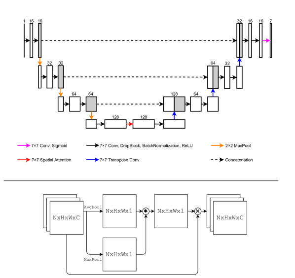
The model employed for this study is Spatial-Attention U-Net (SA-UNet), developed by \citeASDUNet,SAUNet. The SA-UNet is featured by a U-Net [Ronneberger \BOthers. (\APACyear2015)] architecture with a spatial attention module at the bottle-neck of the model structure. U-Net has been successful in classifying an image into different labels. With modifications to the U-Net, SA-UNet has been shown that it is capable of identifying vessels from the eyeball images [Guo \BOthers. (\APACyear2020)]. The model implementation is also available on Github (https://github.com/clguo/SA-UNet). Since vessels and ionogram traces are both tiny or elongated features, we consider that SA-UNet is suitable for the ionogram recovery.
The architecture of the SA-UNet is shown in Figure 3. When an ionogram is sent through the model, the convolution block extracts the features, and the pooling layer reduce the image size. The DropBlock [Ghiasi \BOthers. (\APACyear2018)] randomly drops the image pixels to virtually increase the sample size, which can potentially reduce the overfitting. The spatial attention module rescales the features, so that the model can put more emphasis on important features. The features extracted are assembled and localized in the transpose convolution blocks. The skip-connections return the image size back to the original size. The last convolution layer outputs the probability of the seven signal labels at each pixel. The probability of each label is rounded to a binary value. Since the activation in the last layer is a sigmoid function, which does not normalize the output probability, the model retains the capability of predicting multiple labels for a same pixel. The drop rate of the DropBlock in the original SA-UNet is calculated as follows:
| (1) |
where is the drop rate, is the kernel size, is the height of the image, is the width of the image, and is the probability to keep the kernel. To reduce the computational complexity, we slightly modified the above formula of drop rate to the following:
| (2) |
3.2 Model Training, Evaluation and Optimization
In each training epoch, a mini-batch is fed into the model, and the loss is obtained by calculating the binary crossentropy between the ground truth and the prediction. The model weights are then updated by backpropagating the gradients obtained by the AMSGrad optimizer [Reddi \BOthers. (\APACyear2019)]. An epoch is completed after all mini-batches are used up. The learning rate is set to initially, and is halved until it reaches a minimum rate of if no improvement of the loss of the validation data is found from the previous epochs. A final model is selected from all the epochs by manually checking the performance of the validation set. We found no significant improvement after epochs.
We measure the model performance by the intersection over union (IoU). We modify the definition of IoU in order to apply this to labels. The IoU of each label in an individual ionogram , is computed as the ratio of the total number of intersecting pixels of the ground truth and the prediction () over the total number of union pixels of ground truth and prediction (). The mean IoU of each label , , is computed as the sum of the intersecting pixels over the sum of the union pixels of all ionograms. The equations for IoUn,k and mean IoUk are as follows:
| (3) | |||||
| (4) | |||||
The mean IoU is calculated in such a way that we do not encounter zero-division for labels with both and . An example of application of this technique is shown in Figure 5 (see Section 4.1).
The model is optimized by tuning the hyperparameters. In this study, the hyperparameter includes the size of the convolution kernel, the keep probability of DropBlock, the size of the mini-batch. The default hyperparameters are kernel size of , keep probability of , and batch-size of . To prevent a large searching grid, the hyperparameter is tuned individually while the others are fixed to their default values. The size of the convolution kernel varies between , , and ; the keep probability varies between , , and ; the size of the mini-batch varies between , , , and . This results in different combinations of hyperparameters. By manually comparing the IoUs of the validation data from the combinations of hyperparameters, we determine the optimal hyperparameters as kernel sizes of , and the batch size of . We found the optimal performance occurs at the th epoch.
4 Result
4.1 Recovery of Ionogram Signals
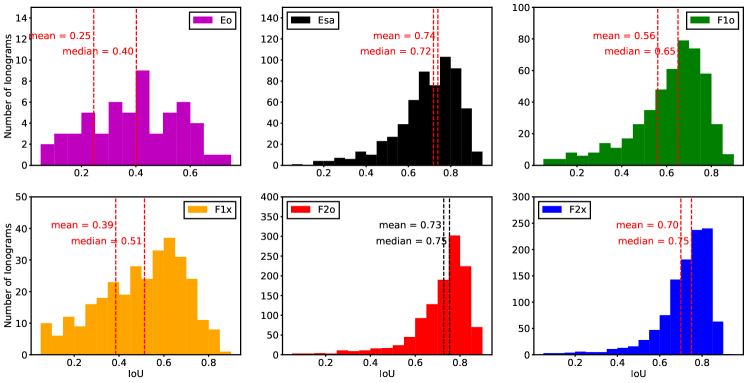
The distribution of IoUs of each label in the test set is plotted in Figure 4 with the mean IoU printed in the corresponding panels. The figure shows that the most accurately recovered signals by SA-UNet are Esa, F2o, and F2x, with mean IoUs reaching approximately . F1o and F1x are less well recovered, with mean IoU equal to and , respectively. The near-zero mean IoU of Eo and Ex indicates that the model cannot identify these two signals. Comparing the mean IoUs of different labels and their coverage ratio in the training set (Table 1) indicates that the two are highly related: The labels with coverage ratio over are the best recovered labels, and the two labels, Eo and Ex, with the lowest coverage ratios are the worst recovered.
A notable amount of zero IoUs are observed. We divide these zero IoUs into three different types (see Table 2).
| Eo | Ex | Esa | F1o | F1x | F2o | F2x | |
|---|---|---|---|---|---|---|---|
| Test set | 83 | 10 | 638 | 490 | 339 | 1160 | 1083 |
| Zero IoUs | 52 | 10 | 36 | 114 | 209 | 22 | 88 |
| FN | 28 | 10 | 14 | 3 | 11 | 3 | 1 |
| FFP | 17 | 0 | 9 | 16 | 95 | 9 | 52 |
| FP | 7 | 0 | 13 | 95 | 103 | 10 | 35 |
-
1.
Model fails to identify correctly labeled signals (false negative, FN): This happens when the model either fails to identify the signal or incorrectly identities it as other labels. Such situation commonly occurs for the signals with low coverage ratio, which can result in model being undertrained. In fact, all Ex instances in ionograms are identified as Eo label.
-
2.
Model correctly identifies the signals that are not labeled (false false-positive, FFP): This happens when the model correctly identifies the signals that were not labeled or incorrectly labeled. The signals that are overlapping with other signals or are contaminated by strong noise are difficult for human to accurately label them. The correct identification of such signals by our model indicates its superior capability over human eye. One such example can be seen in Figure 5a: there is a tiny Eo signal in the ionogram that was incorrectly labeled as Esa due to strong noise. The model correctly separates the signal into increasing (Eo) and the decreasing (Esa) part, resulting in zero IoU for Eo and lower IoU for Esa.
-
3.
Model incorrectly identifies the signals that do not exist (false positive; FP): Such situation occurs when the model is overtrained to a specific label, thus trying to identify too many unrelated pixels as the label. For example, in panel (b) of Figure 5, there are only F2o and F2x signals labeled in the ground truth data, but the model divides the beginning parts of F2o and F2x as F1o and F1x signals.
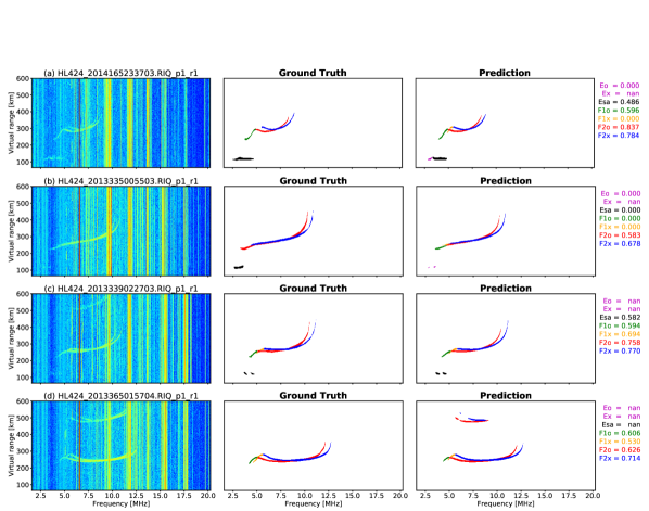
In addition to different types of zero IoUs, mean IoU can also be decreased by echo signals being identified as the primary ones. Echo signals are the signals bouncing between the ground and the ionosphere. In the ionograms, they have similar shapes as the main signals, but appear at higher altitudes with weaker amplitudes. As shown in panel (c) of Figure 5, the model correctly identifies the signals from the ionosonde measurement. However, in panel (d), the echo signals at higher altitude are also identified by the model as F2o and F2x labels, lowering their IoUs as a result.
To investigate the local time and the seasonal dependency of the model performance, we consider the median value of IoU, and use the first and the third quartiles as the error bar. The panels in Figure 6a show the local time variation of IoUs of Eo, Esa, F1o, F1x, F2o, and F2x of the test. Apart from 23:00, the median value of IoU of Esa, F2o, and F2x labels in general are independent of the local time. The panels in Figure 6b show the seasonal variation of the IoUs. The IoUs of F1 (F2o) and F2 (F2o and F2x) layers have a tendency to decrease in the summer, while the IoU of Esa label increases. This could be caused by non-uniform statistics of the layers. Namely, sporadic Es has higher occurrence and intensity during summer months. Strong Es layer very often hide the F2 layer such that the statistics of those labels decrease in summer [Mendoza \BOthers. (\APACyear2021)].
4.2 Examination of Ionogram Parameters
From the ionograms recovered by the deep learning model, we extract the virtual heights, the critical frequencies and the intersection frequencies by an automated procedure. In this study, we only present the parameters for F2 signals, because our model performs the best on F2 signals. The same analysis can also be applied to other signals. For a signal X in the -th recovered ionogram, at frequency and virtual height is defined as:
| (5) |
The virtual height of the F2 signal is defined as the minimum of where F2o is non-zero:
| (6) |
and the critical frequencies foF2 and fxF2 are defined as the maximum of at which F2o and F2x are non-zero:
| (8) | |||||
| (9) |
and the intersection frequency between the F2o and the F2x signals, is defined as the first intersection point from the high frequency.
| (10) |
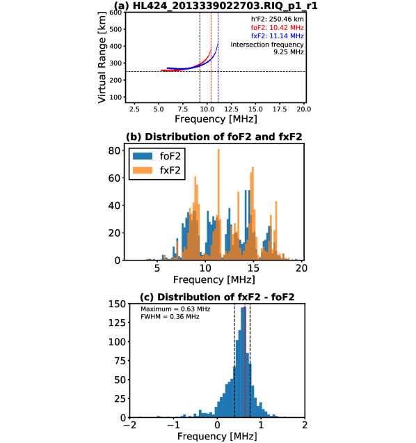
For F2o and F2x signals with large overlapping area, the extracted intersection frequency is not reliable and cannot be used. We consider the overlapping area greater than of their combined area as highly overlapped. Out of ionograms recovered from the test set, are below the threshold. One example is shown in Figure 7a. The corresponding original ionogram is measured at 2013/12/05 02:27:03, the same timestamp as the ionogram in Figure 5c. For this timestamp, the virtual height of F2 is km, the critical frequencies foF2 and fxF2 are MHz, and MHz, respectively, and the intersection frequency between the F2o signal and the F2x signal is MHz.
The distributions of foF2 and fxF2 are plotted in Figure 7b. It shows that the extracted foF2 varies from MHz to MHz. The distribution of the difference between fxF2 and foF2 (fxF2foF2) is shown in Figure 7c. It shows a distribution close to a Gaussian profile, with a tail on the left-hand side. The peak of the distribution is MHz, and the full-width half-maximum (FWHM) is MHz, making the uncertainty of the difference (FWHM) to be MHz.
5 Discussion
Studies have shown that the deep learning models are able to scale the ionograms automatically. The reported performance of the deep learning models are summarized and compared with our result in Table 3. \citeAaeperu applied the Autoencoder model (denoted by the superscript a) to extract F region signals from Peru’s ionograms, and obtained IoU for the combined F layer signals (F1 F2), after fine-tuning the model parameters. The Fully Convolutional DenseNet model (denoted by the superscript b) used in \citeAsnr to recover the ionospheric signals obtained an IoU of nearly for Esa and F2o layers. \citeAunetseg used multiple U-Net models (denoted by the superscript c) to scale E, F1, F2 layers, and obtained the dice-coefficient loss (DCL) of , , and for E, F1 and F2 layers, respectively, in the ionograms of 64x48 pixels, and , , and in the ionograms of 192x144 pixels. Note that a smaller DCL indicates a better performance. Our SA-UNet model, applied to highly noisy ionograms of 800x1600 pixels, achieves an IoU and DCL score for Esa and F2 layers. To provide additional information for interested readers, we also list the recall rates and precision rates achieved by our model, which are calculated by counting the pixel number of true positives, false positives, and false negatives. It should be noted that the ionograms used by \citeAaeperu and \citeAunetseg have been obtained either at middle latitudes or/and in the remote regions with low man-made signals. In short, our study shows that the SA-UNet can improve the performance to IoU and reduce DCL to below 0.18.
| Size (HxW) | Metric | Eo | Ex | Esa | F1o | F1x | F2o | F2x | |
| Autoencodera | 256x208 | IoU | N/A | N/A | N/A | 0.60 | |||
| FC-DenseNetb | 800x1600 | IoU | 0.00 | 0.00 | 0.56 | 0.47 | 0.33 | 0.59 | 0.48 |
| U-Netc | 64x48 | DCL | 0.16 | 0.17 | 0.11 | ||||
| 192x144 | DCL | 0.22 | 0.23 | 0.19 | |||||
| SA-UNet | 800x1600 | IoU | 0.25 | 0.00 | 0.74 | 0.56 | 0.39 | 0.73 | 0.70 |
| Recall | 0.28 | 0.00 | 0.85 | 0.73 | 0.51 | 0.83 | 0.83 | ||
| Precision | 0.68 | N/A | 0.85 | 0.71 | 0.61 | 0.86 | 0.82 | ||
| DCL | 0.61 | 1.00 | 0.15 | 0.28 | 0.44 | 0.16 | 0.18 | ||
The critical frequency foF2 is directly related to the maximum number density of electrons in F2 layer, and the difference between fxF2 and foF2 can provide an estimation of the local geomagnetic field [Piggott \BBA Rawer (\APACyear1978)]:
| (11) | |||||
| (12) |
Our results show that the derived electron number density ranges from m-3 to m-3, and the magnetic field is G. Since the local variation of the geomagnetic field is usually small, the large uncertainty of the magnetic field is likely caused by strong noises in the ionograms. We also find 76 recovered ionograms with foF2 fxF2. They are caused by both false positive and false negative predictions.
The existence of echoes does not affect the extraction of critical frequencies. However, cares should be taken for extracting the critical virtual heights. In addition to the local geomagnetic field, the difference between foF2 and fxF2 can also be used to estimate foF2 (i.e. ) in the case when fxF2 is obtained but F2o cannot be accurately recovered.
The intersection frequency can be used for the verification of the ordinary and extra-ordinary signals from the F2 layer. Namely, the ascending branch of the ordinary signal should be situated at lower frequencies than the extra-ordinary one. This technique can provide a robust correction of inaccurate model predictions of the signals from the F2 layer and, thus, more accurate determination of the critical frequencies foF2 and fxF2.
The low percentages of Eo and Ex labels in the training, validation and the test set could bias the model performance. In order to generalize the data representation, an k-fold or a leave-one-out cross validation may be applied [Love \BOthers. (\APACyear2020), Nishizuka \BOthers. (\APACyear2021)]. Moreover, there are a few techniques which may reduce the class imbalance problem, such as undersampling/oversampling to the training set [Lemaître \BOthers. (\APACyear2017)], loss weighted according to the amount of the labels [Raptis \BOthers. (\APACyear2020), Aminalragia-Giamini \BOthers. (\APACyear2021)], transfer learning from a larger dataset, or ensemble learning of multiple models, to name a few.
It is important to note that the present dataset spans less than one year, and includes only ionospheric statistics at low latitudes under very dynamic region of the bulge of equatorial ionization anomaly. The ionosphere dynamics depends on latitude and varies with solar and geomagnetic activity. Hence, to enable the application of our model to other datasets, the model should be trained on the combination of different data set. Alternatively, the transfer learning technique can be applied to reduce the training time and improve the model performance on a different data set.
6 Conclusions
In this study, we show that SA-UNet is capable of recovering F2o and F2x signals, and the Esa label (which is a combination of Eso, Esx, and Es signals) from the highly contaminated Hualien VIPIR measurements. While the performance of identifying Eo and Ex is poor due to the class imbalance, their low percentage in the statistics suggests that they have little effect on the ionosphere in the Taiwan region. By comparing the input ionogram, ground truth labeling, and the model prediction, our results show that the model is capable of recovering signals that are not labeled, due to contamination by strong noise or overlapping with another signal. The recovered ionograms can be further used in extracting the virtual height, the critical frequency and the intersection frequency of different labels, which are important in the determination of the electron density profile and the magnetic field of the ionosphere overhead.
7 Open Research
The ionogram data and the model used in this study can be openly accessed on Kaggle. The link for the data is provided as follows: https://www.kaggle.com/changyuchi/ncu-ai-group-data-set-fcdensenet24. The link for the model is provided as follows: https://www.kaggle.com/guanhanhuang/ncu-ai [G\BHBIH. Huang \BOthers. (\APACyear2022)]. The model is constructed using Tensorflow 2.3 [Abadi \BOthers. (\APACyear2015)] and its Keras packages, and is trained on Kaggle under the GPU computation environment.
Acknowledgements.
This work is funded by the Ministry of Science and Technology of Taiwan under the grant number 109-2923-M-008-001-MY2 and 109-2111-M-008-002. The figures are made by using the Matplotlib package [Hunter (\APACyear2007)].References
- Abadi \BOthers. (\APACyear2015) \APACinsertmetastartensorflow{APACrefauthors}Abadi, M., Agarwal, A., Barham, P., Brevdo, E., Chen, Z., Citro, C.\BDBLZheng, X. \APACrefYearMonthDay2015. \APACrefbtitleTensorFlow: Large-Scale Machine Learning on Heterogeneous Systems. TensorFlow: Large-scale machine learning on heterogeneous systems. {APACrefURL} https://tensorflow.org/ \APACrefnoteAccessed on 1 June 2022 \PrintBackRefs\CurrentBib
- Aminalragia-Giamini \BOthers. (\APACyear2021) \APACinsertmetastarwtloss2{APACrefauthors}Aminalragia-Giamini, S., Raptis, S., Anastasiadis, A., Tsigkanos, A., Sandberg, I., Papaioannou, A.\BDBLDaglis, I\BPBIA. \APACrefYearMonthDay2021\APACmonth11. \BBOQ\APACrefatitleSolar Energetic Particle Event occurrence prediction using Solar Flare Soft X-ray measurements and Machine Learning Solar Energetic Particle Event occurrence prediction using Solar Flare Soft X-ray measurements and Machine Learning.\BBCQ \APACjournalVolNumPagesJournal of Space Weather and Space Climate1159. {APACrefDOI} 10.1051/swsc/2021043 \PrintBackRefs\CurrentBib
- Ghiasi \BOthers. (\APACyear2018) \APACinsertmetastarDropBlock1{APACrefauthors}Ghiasi, G., Lin, T\BHBIY.\BCBL \BBA Le, Q\BPBIV. \APACrefYearMonthDay2018. \APACrefbtitleDropBlock: A regularization method for convolutional networks. Dropblock: A regularization method for convolutional networks. \APACaddressPublisherarXiv. {APACrefURL} https://arxiv.org/abs/1810.12890 {APACrefDOI} 10.48550/ARXIV.1810.12890 \PrintBackRefs\CurrentBib
- Guo \BOthers. (\APACyear2019) \APACinsertmetastarSDUNet{APACrefauthors}Guo, C., Szemenyei, M., Pei, Y., Yi, Y.\BCBL \BBA Zhou, W. \APACrefYearMonthDay2019. \BBOQ\APACrefatitleSD-Unet: A Structured Dropout U-Net for Retinal Vessel Segmentation Sd-unet: A structured dropout u-net for retinal vessel segmentation.\BBCQ \BIn \APACrefbtitle2019 IEEE 19th International Conference on Bioinformatics and Bioengineering (BIBE) 2019 ieee 19th international conference on bioinformatics and bioengineering (bibe) (\BPG 439-444). \PrintBackRefs\CurrentBib
- Guo \BOthers. (\APACyear2020) \APACinsertmetastarSAUNet{APACrefauthors}Guo, C., Szemenyei, M., Yi, Y., Wang, W., Chen, B.\BCBL \BBA Fan, C. \APACrefYearMonthDay2020. \BBOQ\APACrefatitleSA-UNet: Spatial Attention U-Net for Retinal Vessel Segmentation Sa-unet: Spatial attention u-net for retinal vessel segmentation.\BBCQ \APACjournalVolNumPagesArXivabs/2004.03696. \PrintBackRefs\CurrentBib
- G\BHBIH. Huang \BOthers. (\APACyear2022) \APACinsertmetastarncuai{APACrefauthors}Huang, G\BHBIH., Dmitriev, A\BPBIV., Tsai, L\BHBIC., Tsogtbaatar, E., Chang, Y\BHBIC., Hsieh, M\BHBIC.\BDBLLin, C\BHBIH. \APACrefYearMonthDay2022. \APACrefbtitleSA-UNet for The Recovery of Ionograms. Sa-unet for the recovery of ionograms. \APACaddressPublisherKaggle. {APACrefURL} https://www.kaggle.com/ds/1933301 \APACrefnoteAccessed on 1 June 2022 {APACrefDOI} 10.34740/KAGGLE/DS/1933301 \PrintBackRefs\CurrentBib
- X. Huang \BBA Reinisch (\APACyear2001) \APACinsertmetastartopside{APACrefauthors}Huang, X.\BCBT \BBA Reinisch, B. \APACrefYearMonthDay2001. \BBOQ\APACrefatitleVertical electron content from ionograms in real time Vertical electron content from ionograms in real time.\BBCQ \APACjournalVolNumPagesRadio Science - RADIO SCI36335-342. {APACrefDOI} 10.1029/1999RS002409 \PrintBackRefs\CurrentBib
- Hui \BOthers. (\APACyear2018) \APACinsertmetastaroxpoint_b{APACrefauthors}Hui, H., Chen, Z., Jiang, C\BHBIH., Yang, G\BHBIB.\BCBL \BBA Zhao, Z\BHBIY. \APACrefYearMonthDay2018. \BBOQ\APACrefatitleMethod for automatic scaling of O wave traces from ionograms Method for automatic scaling of o wave traces from ionograms.\BBCQ \APACjournalVolNumPagesProgress in Geophysics331351-1357. {APACrefDOI} 10.6038/pg2018BB0355 \PrintBackRefs\CurrentBib
- Hunter (\APACyear2007) \APACinsertmetastarmatplotlib{APACrefauthors}Hunter, J\BPBID. \APACrefYearMonthDay2007. \BBOQ\APACrefatitleMatplotlib: A 2D graphics environment Matplotlib: A 2d graphics environment.\BBCQ \APACjournalVolNumPagesComputing in Science & Engineering9390–95. {APACrefDOI} 10.1109/MCSE.2007.55 \PrintBackRefs\CurrentBib
- Jara \BBA Olivares (\APACyear2021) \APACinsertmetastaraeperu{APACrefauthors}Jara, C.\BCBT \BBA Olivares, C. \APACrefYearMonthDay2021. \BBOQ\APACrefatitleIonospheric Echo Detection in Digital Ionograms Using Convolutional Neural Networks Ionospheric echo detection in digital ionograms using convolutional neural networks.\BBCQ \APACjournalVolNumPagesRadio Science56. {APACrefDOI} 10.1029/2020RS007258 \PrintBackRefs\CurrentBib
- Kelley (\APACyear1989) \APACinsertmetastarintro{APACrefauthors}Kelley, M\BPBIC. \APACrefYearMonthDay1989. \BBOQ\APACrefatitleChapter 1 - Introductory and Background Material Chapter 1 - introductory and background material.\BBCQ \BIn M\BPBIC. Kelley (\BED), \APACrefbtitleThe Earth’s Ionosphere The earth’s ionosphere (\BPG 1-22). \APACaddressPublisherAcademic Press. {APACrefURL} https://www.sciencedirect.com/science/article/pii/B978012404013750006X {APACrefDOI} https://doi.org/10.1016/B978-0-12-404013-7.50006-X \PrintBackRefs\CurrentBib
- Lemaître \BOthers. (\APACyear2017) \APACinsertmetastarousampling{APACrefauthors}Lemaître, G., Nogueira, F.\BCBL \BBA Aridas, C\BPBIK. \APACrefYearMonthDay2017jan. \BBOQ\APACrefatitleImbalanced-Learn: A Python Toolbox to Tackle the Curse of Imbalanced Datasets in Machine Learning Imbalanced-learn: A python toolbox to tackle the curse of imbalanced datasets in machine learning.\BBCQ \APACjournalVolNumPagesJ. Mach. Learn. Res.181559–563. \PrintBackRefs\CurrentBib
- Love \BOthers. (\APACyear2020) \APACinsertmetastarcv1{APACrefauthors}Love, T., Neukirch, T.\BCBL \BBA Parnell, C\BPBIE. \APACrefYearMonthDay2020\APACmonth06. \BBOQ\APACrefatitleAnalysing AIA Flare Observations using Convolutional Neural Networks Analysing AIA Flare Observations using Convolutional Neural Networks.\BBCQ \APACjournalVolNumPagesFrontiers in Astronomy and Space Sciences734. {APACrefDOI} 10.3389/fspas.2020.00034 \PrintBackRefs\CurrentBib
- Mendoza \BOthers. (\APACyear2021) \APACinsertmetastarsnr{APACrefauthors}Mendoza, M\BPBIM., Chang, Y\BHBIC., Dmitriev, A\BPBIV., Lin, C\BHBIH., Tsai, L\BHBIC., Li, Y\BHBIH.\BDBLTsogtbaatar, E. \APACrefYearMonthDay2021. \BBOQ\APACrefatitleRecovery of Ionospheric Signals Using Fully Convolutional DenseNet and Its Challenges Recovery of ionospheric signals using fully convolutional densenet and its challenges.\BBCQ \APACjournalVolNumPagesSensors2119. {APACrefURL} https://www.mdpi.com/1424-8220/21/19/6482 {APACrefDOI} 10.3390/s21196482 \PrintBackRefs\CurrentBib
- Mochalov \BBA Mochalova (\APACyear2019) \APACinsertmetastarunetseg{APACrefauthors}Mochalov, V.\BCBT \BBA Mochalova, A. \APACrefYearMonthDay2019. \BBOQ\APACrefatitleExtraction of ionosphere parameters in ionograms using deep learning Extraction of ionosphere parameters in ionograms using deep learning.\BBCQ \APACjournalVolNumPagesE3S Web Conf.12701004. {APACrefDOI} 10.1051/e3sconf/201912701004 \PrintBackRefs\CurrentBib
- Nishizuka \BOthers. (\APACyear2021) \APACinsertmetastarcv2{APACrefauthors}Nishizuka, N., Kubo, Y., Sugiura, K., Den, M.\BCBL \BBA Ishii, M. \APACrefYearMonthDay2021\APACmonth12. \BBOQ\APACrefatitleOperational solar flare prediction model using Deep Flare Net Operational solar flare prediction model using Deep Flare Net.\BBCQ \APACjournalVolNumPagesEarth, Planets and Space73164. {APACrefDOI} 10.1186/s40623-021-01381-9 \PrintBackRefs\CurrentBib
- Piggott \BBA Rawer (\APACyear1978) \APACinsertmetastarhandbook{APACrefauthors}Piggott, W\BPBIR.\BCBT \BBA Rawer, K. \APACrefYear1978. \APACrefbtitleU.R.S.I. Handbook of Ionogram Interpretation and Reduction U.r.s.i. handbook of ionogram interpretation and reduction (\PrintOrdinal2 \BEd). \APACaddressPublisherNatl. Geophys. Data Cent. Boulder, Colo.World Data Cent. A for Sol.-Terr. Phys. {APACrefURL} https://repository.library.noaa.gov/view/noaa/10404 \PrintBackRefs\CurrentBib
- Pulinets (\APACyear1995) \APACinsertmetastaroxpoint_a{APACrefauthors}Pulinets, S\BPBIA. \APACrefYearMonthDay1995. \BBOQ\APACrefatitleAutomatic vertical ionogram collection, processing and interpretation Automatic vertical ionogram collection, processing and interpretation.\BBCQ \BIn \APACrefbtitleIonosonde network and stations Ionosonde network and stations (\BPG 37-43). \APACaddressPublisherBoulder, Colo.World Data Cent. \PrintBackRefs\CurrentBib
- Raptis \BOthers. (\APACyear2020) \APACinsertmetastarwtloss1{APACrefauthors}Raptis, S., Aminalragia-Giamini, S., Karlsson, T.\BCBL \BBA Lindberg, M. \APACrefYearMonthDay2020\APACmonth06. \BBOQ\APACrefatitleClassification of Magnetosheath Jets UsingNeural Networks and High Resolution OMNI(HRO) Data Classification of Magnetosheath Jets UsingNeural Networks and High Resolution OMNI(HRO) Data.\BBCQ \APACjournalVolNumPagesFrontiers in Astronomy and Space Sciences724. {APACrefDOI} 10.3389/fspas.2020.00024 \PrintBackRefs\CurrentBib
- Reddi \BOthers. (\APACyear2019) \APACinsertmetastaramsgrad{APACrefauthors}Reddi, S\BPBIJ., Kale, S.\BCBL \BBA Kumar, S. \APACrefYearMonthDay201904. \APACrefbtitleOn the Convergence of Adam and Beyond. On the convergence of adam and beyond. \PrintBackRefs\CurrentBib
- Ronneberger \BOthers. (\APACyear2015) \APACinsertmetastarunet{APACrefauthors}Ronneberger, O., Fischer, P.\BCBL \BBA Brox, T. \APACrefYearMonthDay2015. \APACrefbtitleU-Net: Convolutional Networks for Biomedical Image Segmentation. U-net: Convolutional networks for biomedical image segmentation. \PrintBackRefs\CurrentBib
- Shinagawa \BOthers. (\APACyear2021) \APACinsertmetastare_summer{APACrefauthors}Shinagawa, H., Tao, C., Jin, H., Miyoshi, Y.\BCBL \BBA Fujiwara, H. \APACrefYearMonthDay2021\APACmonth12. \BBOQ\APACrefatitleNumerical prediction of sporadic E layer occurrence using GAIA Numerical prediction of sporadic E layer occurrence using GAIA.\BBCQ \APACjournalVolNumPagesEarth, Planets and Space73128. {APACrefDOI} 10.1186/s40623-020-01330-y \PrintBackRefs\CurrentBib
- Titheridge (\APACyear1988) \APACinsertmetastartrue_height_1{APACrefauthors}Titheridge, J\BPBIE. \APACrefYearMonthDay1988. \BBOQ\APACrefatitleThe real height analysis of ionograms: A generalized formulation The real height analysis of ionograms: A generalized formulation.\BBCQ \APACjournalVolNumPagesRadio Science235831-849. {APACrefURL} https://agupubs.onlinelibrary.wiley.com/doi/abs/10.1029/RS023i005p00831 {APACrefDOI} https://doi.org/10.1029/RS023i005p00831 \PrintBackRefs\CurrentBib
- Tsai \BBA Berkey (\APACyear2000) \APACinsertmetastarfuzzy{APACrefauthors}Tsai, L\BHBIC.\BCBT \BBA Berkey, F\BPBIT. \APACrefYearMonthDay2000. \BBOQ\APACrefatitleIonogram analysis using fuzzy segmentation and connectedness techniques Ionogram analysis using fuzzy segmentation and connectedness techniques.\BBCQ \APACjournalVolNumPagesRadio Science3551173-1186. {APACrefDOI} 10.1029/1999RS002170 \PrintBackRefs\CurrentBib
- Tsai \BOthers. (\APACyear1995) \APACinsertmetastartrue_height_2{APACrefauthors}Tsai, L\BHBIC., Berkey, F\BPBIT.\BCBL \BBA Stiles, G\BPBIS. \APACrefYearMonthDay1995. \BBOQ\APACrefatitleThe true-height analysis of ionograms using simplified numerical procedures The true-height analysis of ionograms using simplified numerical procedures.\BBCQ \APACjournalVolNumPagesRadio Science304949-959. {APACrefDOI} 10.1029/95RS00936 \PrintBackRefs\CurrentBib
- Wada (\APACyear2016) \APACinsertmetastarlabelme{APACrefauthors}Wada, K. \APACrefYearMonthDay2016. \APACrefbtitlelabelme: Image Polygonal Annotation with Python. labelme: Image Polygonal Annotation with Python. \APAChowpublishedhttps://github.com/wkentaro/labelme. \PrintBackRefs\CurrentBib
- Xiao \BOthers. (\APACyear2020) \APACinsertmetastardias{APACrefauthors}Xiao, Z., Wang, J., Li, J., Zhao, B., Hu, L.\BCBL \BBA Liu, L. \APACrefYearMonthDay2020. \BBOQ\APACrefatitleDeep-learning for ionogram automatic scaling Deep-learning for ionogram automatic scaling.\BBCQ \APACjournalVolNumPagesAdvances in Space Research664942-950. {APACrefURL} https://www.sciencedirect.com/science/article/pii/S027311772030332X {APACrefDOI} https://doi.org/10.1016/j.asr.2020.05.009 \PrintBackRefs\CurrentBib