Gravitational Contact Interactions —
— Does the Jordan Frame Exist?
In Honor of Graham G. Ross

Abstract

Scalar–tensor theories, with Einstein Hilbert and non-minimal interactions, $\sim M^{2}R/2-\alpha\phi^{2}R/12$, have graviton exchange induced contact interactions. These always pull the theory back into a formal Einstein frame in which $\alpha$ does not exist. In the Einstein frame, contact terms are induced, that are then absorbed back into other couplings to define the effective potential (or equivalently, the renormalization group). We show how these effects manifest themselves in a simple model by computing the effective potential in both frames displaying the discrepancy.

I Introduction

Today we are here to honor the life and career of our colleague, Graham Ross. I’ve known Graham for nearly 50 years, beginning at Caltech when I was a graduate student in the mid-1970’s and he was a Research Scientist. He became a mentor and good friend.

Back then, we worked on the new theory, QCD, exploring the photon structure functions, photon , and nonleptonic weak interactions, nonleptonic , with renormalization group (RG) methods. In the latter we followed the pioneering work of Shifman , where I was first introduced to “contact interactions” via the so-called “penguin diagrams” (so named in ref.penguins ). Contact interactions will play a central role in my talk today.

In 1981, I visited Oxford where Graham had joined the faculty. There we discussed the possibility that the top quark would be very heavy. He had some ideas based upon the RG equation for the top quark Yukawa coupling, $g_{top}$. He proposed that $g_{top}/g_{QCD}$ would flow into the infra-red to a fixed ratio (a tracker solution), which predicted a top quark mass of about 110 GeV (with Brian Pendleton PR ). Note that at this time the experimental limit on the top quark mass was of order $\sim 10$ GeV, and most people believed it would appear at about $\sim 3\times m_{b}\sim 15$ GeV.

Inspired by the Pendleton-Ross idea, I studied the RG equations and found the predicted top quark mass would most probably be near an “infrared quasi-fixed point,” or “focus point,” $\sim 220$ GeV fixed assuming standard model running to the high scales. People were quite skeptical, however, about a heavy top quark (some people promised to “eat their hats” if the top mass exceeded $\sim 40-90$ GeV but I don’t recall beholding any such feasts). In the late 1980’s Graham and I overlapped at CERN for a year and we worked on various generalizations of axions schiz , which, particularly in the neutrino sector, proved to have potentially interesting cosmological implications late .

In the 1990’s it was becoming clear that the top quark was surprisingly heavy. Bardeen, Lindner and I considered a composite Higgs boson as a boundstate of top and anti-top quarks BHL . We found that the composite solution implied that $g_{top}$ should be near the RG quasi–fixed point value, inspired from the work of Pendleton and Ross a decade earlier. The top quark finally weighed in at the Tevatron in 1995 at $175$ GeV, shy of fixed point prediction by about 20%. I remain of the opinion that this is suggesting an intimate dynamical relationship between the top quark and Higgs boson, though we may not yet have the full theory (see CTH3 for a sketch of some new ideas).

Graham Ross was a universal physicist, able to move from phenomenology to theory comfortably. Above all, he paid close attention to experimental results. He was a key player in developing many ideas surrounding the MSSM in the ‘80’s and ‘90’s. However, circa 2014 he became increasingly interested in alternatives, such as the Weyl invariant gravity theories which had become an active arena of research Weyl ; authors ; HillRoss ; staro . We then renewed our collaboration, and that carried us to his untimely passing.

I feel a great loss, of a dear friend and colleague, an amiable person of the highest integrity, an energetic researcher with a deep passion for real world physics and its essential interface with experiment, and someone I’ve known for much of my life. We leave a half dozen unfinished papers on our laptops.

I would like to talk today about one of my more recent works with Graham Ross, because I feel it is foundational to quantum field theory and model independent. This work came out of the Covid pandemic, and we had daily multiple email exhanges, sometime skype calls, during this time.

The subject of my talk is the field theoretic structure of non-minimal gravitationally coupled scalars in the regime in which the Planck mass is present (as opposed to any putative pre-Planckian era). The question that emerges from this is: “Does the Jordan frame really exist?” You’ll see what I think as the story unfolds. All of this is described in the paper HillRoss , and some of the implications are tackled in staro . A follow-on paper with one of Graham’s former students, Dumitru Ghilencea, is nearing completion Ghil .

II Non-Minimal Couplings of Scalars to Curvature

Over the years there has been considerable interest in Brans-Dicke, scalar-tensor, and scale or Weyl invariant theories. These have in common fundamental scalar fields, $\phi_{i}$, that couple to gravity through non-minimal interactions, $\sim M^{2}R+F(\phi_{i})R$. The Planck mass, $M$ can co-exist with these non-minimal couplings, or the scalars may acquire VEV’s that dynamically generate it authors . When the theory is proscribed with non–minimal interactions we say it is given in a “Jordan frame.”

A key tool in the analysis of these models is the Weyl transformation, Weyl . This involves a redefinition of the metric, $g^{\prime}=\Omega(\phi_{i})g$, in which $g$ comingles with the scalars. $\Omega$ can be chosen to lead to a new effective theory, typically one that has a pure Einstein-Hilbert action, $\sim M^{2}R$, in which the non-mimimal interactions have been removed. This is called the “Einstein frame.” Alternatively, one might use a Weyl transformation to partially remove a subset of scalars from the non-minimal interactions $\sim M^{2}R+F^{\prime}(\phi_{i})R$, where $F^{\prime}$ is optimized for some particular application.

It is a priori unclear, however, how or whether the original Jordan frame theory can be physically equivalent to the Einstein frame form and how the Weyl transformation is compatible with a full quantum theory Duff Ruf . Nonetheless, many authors consider this to be a valid transformation and a symmetry of Weyl invariant theories, and many loop calculations permeate the literature which attempt to exploit apparent simplifications offered by the Jordan frame.

Graham Ross and I showed that any theory with non-minimal couplings contains contact terms HillRoss . These are generated by the graviton exchange amplitudes in tree approximation and they are therefore ${\cal{O}}(\hbar^{0})$ and therefore classical. The contact terms occur because emission vertices from the non-minimal interaction are proportional to $q^{2}$ of the graviton, while the Feynman propagator is proportional to $1/q^{2}$. The cancellation of $q^{2}\times 1/q^{2}$ therefore leads to point-like interactions that must be included into the effective action of the theory at any given order of perturbation theory. The result is that the non-minimal interactions disappear from the theory and Planck suppressed higher dimension operators appear with modified couplings.

The structural form of the theory when the contact term interactions are included corresponds formally to a Weyl transformation of the metric that takes the theory to the pure Einstein frame with higher dimension, Planck suppressed, interactions. In the pure Einstein-Hilbert action there are no classical contact terms, but at loop level they can be generated, and must be removed as part of the renormalization group. However, by virtue of the contact terms, nowhere is a metric redefinition performed (hence the issue of a Jacobian in the measure of the gravitational path integral in going to the Einstein frame becomes moot).

This means that, provided we are interested in the theory on mass scales below $M$, the Jordan frame is an illusion and doesn’t really exist physically. In the Jordan frame the contact terms are hidden, but they are always present, ergo, even though the action superficially appears to be Jordan, it isn’t, and remains always in an Einstein frame.

Efforts to compute quantities, such as effective potentials (or equivalently, $\beta$-functions), in the Jordan frame, while ignoring the contact terms, will yield incorrect results. Nonetheless, though the non-minimal interactions are not present in the classical Einstein frame, they are regenerated by loops and the potentials and RG equations are modified by this effect.

In a simple theory in the Jordan frame, where the nonminimal coupling is $-\alpha\phi^{2}R/12$, this raises the question of how to understand the fate of $\alpha$? With a single scalar with quartic and other interactions, $\lambda_{i}$, the usual “naive” calculation of a $\beta$-function in the Jordan frame (“naive” means ignoring contact terms) yields the form:

$$\frac{\partial\alpha(\mu)}{\partial\ln(\mu)}=\beta_{\alpha}(\lambda_{i})\equiv(1-\alpha)\gamma_{\alpha}(\lambda_{i})$$ (1)

where the factor $(1-\alpha)$ reflects the fact that when $M^{2}=0$ and $\alpha=1$ (conformal limit) the kinetic term of $\phi$ disappers and $\phi$ becomes static parameter).

However, the contact terms (or a Weyl tranformation) remove $\alpha$ and leave an Einstein frame with only the Einstein-Hilbert term, $M^{2}R$ and the $\phi$ couplings $\lambda_{i}^{\prime}$ (in what follows primed couplings refer the Einstein frame and un-primed to Jordan frame). This means that $N$ couplings, $(\alpha,\lambda_{i})$, in the Jordan frame have become $N-1$ couplings, $(\lambda_{i}^{\prime})$, in the Einstein frame. Therefore any physical meaning ascribed to $\alpha$ or the $\beta_{\alpha}$ function is apparantly lost.

Three Feynman diagrams (shown below as D1, D2, D3, in Figs.(2,3,4)) contribute to $\beta_{\alpha}$ in the Jordan frame. One of them multiplies $\alpha$ in the Jordan frame (D3) and yields the $(1-\alpha)$ factor in eq.(1). But even with $\alpha=0$ in the Einstein frame, two diagrams (D1 and D2) exist and reintroduce a perturbative $\delta\alpha$, for a small step in scale $\delta\mu/\mu$. This is then removed by the contact terms, but leads to correction terms in the renormalization of the $\lambda_{i}^{\prime}$. We are therefore sensitive to the same scale breaking information in the Einstein frame that one has in the Jordan frame, which is encoded into $\gamma_{\alpha}$. This does not, however, imply that the resulting calculations in the Jordan and Einstein frames are then consistent! I will explicitly demonstrate the inconsistency through calculation pf effective potentials (the RG equations of the couplings can always be read off from the effective potentials).

If we stayed in the Jordan frame, with nonzero $\alpha$, and naively computed the same effective potential (“naively” means ignoring contact terms), into an Einstein frame, we would obtain a different result. The difference is a term proportional to $\alpha$ in the Jordan frame. Equivalently, going initially to the Einstein frame and running with the RG, does not commute with running initially in the Jordan frame and subsequently going to the Einstein frame!

We turn presently to a brief discussion of contact terms in general and review a simple toy model from HillRoss that is structurally similar to the gravitational case. We then summarize gravitational contact terms (and refer the reader to HillRoss for details). We then exemplify the Einstein frame renormalization group compared to the naive Jordan frame result, which ignores contact terms, and illustrate the discrepancy.

III Contact Interactions

Generally speaking “contact interactions” are point-like operators that are generated in the effective action of the theory in perturbation theory. They may arise in the UV from ultra-heavy fields that are integrated out, such as the Fermi weak interaction that arises from integrating out the heavy $W$-boson. They may also arise in the IR when a vertex in the theory is proportional to $q^{2}$ and cancels against a $1/q^{2}$ propagator. The gravitational contact term we discuss presently is of the IR form.

III.1 Contact Terms in Non-gravitational Physics

Contact terms arise in a number of phenomena. Diagrammatically they can arise in the IR when a vertex for the emission of, e.g., a massless quantum, of momentum $q_{\mu}$, is proportional to $q^{2}$. This vertex then cancels the $1/q^{2}$ from a massless propagator when the quantum is exchanged. This $q^{2}/q^{2}$ cancellation leads to an effective pointlike operator from an otherwise single-particle reducible diagram.

For example, in electroweak physics a vertex correction by a $W$-boson to a massless gluon emission induces a quark flavor changing operator, e.g., describing $s\rightarrow d$+gluon, where $s(d)$ is a strange (down) quark. This has the form of a local operator:

$$g\kappa\overline{s}\gamma_{\mu}T^{A}d_{L}D_{\nu}G^{A\mu\nu}$$ (2)

where $G^{A\mu\nu}$ is the color octet gluon field strength and $\kappa\propto G_{Fermi}$.

This implies a vertex for an emitted gluon of 4-momentum $q$ and polarization and color, $\epsilon^{A\mu}$, of the form $g\kappa\overline{s}\gamma_{\mu}T^{A}d_{L}\epsilon^{A\mu}\times q^{2}+...$. However, the gluon propagates, $\sim 1/q^{2}$, and couples to a quark current $\sim g\epsilon^{A\mu}\overline{q}\gamma_{\mu}T^{A}q$. This results in a contact term:

$$g^{2}\kappa\left(\frac{q^{2}}{q^{2}}\right)\overline{s}\gamma^{\mu}T^{A}d_{L}\overline{q}\gamma_{\mu}T^{A}q\;=\;g^{2}\kappa\overline{s}\gamma^{\mu}T^{A}d_{L}\overline{q}\gamma_{\mu}T^{A}q$$

The result is a 4-body local operator which mediates electroweak transitions between, e.g., kaons and pions Shifman , also known as “penguin diagrams” penguins . Note the we can rigorously obtain the contact term result by use of the gluon field equation within the operator of eq.(2),

$$D_{\nu}G^{A\mu\nu}=g\overline{q}\gamma^{\mu}T^{A}q.$$ (4)

This is justified as operators that vanish by equations of motion, known as “null operators,” will generally have gauge noninvariant anomalous dimensions and are unphysical Deans .

Another example occurs in the case of a cosmic axion, described by an oscillating classical field, $\theta(t)=\theta_{0}\cos(m_{a}t)$, interacting with a magnetic moment, $\vec{\mu}(x)\cdot\vec{B}$, through the electromagnetic anomaly $\kappa\theta(t)\vec{E}\cdot\vec{B}$. A static magnetic moment emits a virtual spacelike photon of momentum $(0,\vec{q})$. The anomaly absorbs the virtual photon and emits an on-shell photon of polarization $\vec{\epsilon}$, inheriting energy $\sim m_{a}$ from the cosmic axion. The Feynman diagram, with the exchanged virtual photon, yields an amplitude, $\propto(\theta_{0}\mu^{i}\epsilon_{ijk}q^{j})(1/\vec{q}^{\;2})(\kappa\epsilon^{k\ell h}q_{\ell}m_{a}\epsilon_{h})\sim(\kappa\theta_{0}m_{a}\vec{q}^{\;2}/\vec{q}^{\;2})\vec{\mu}\cdot\vec{\epsilon}$. The $\vec{q}^{\;2}$ factor then cancels the $1/\vec{q}^{\;2}$ in the photon propagator, resulting in a contact term which is an induced, parity violating, oscillating electric dipole interaction: $\sim\kappa\theta(t)\vec{\mu}\cdot\vec{E}$. This results in cosmic axion induced electric dipole radiation from any magnet, including an electron CTHa .

III.2 Illustrative Toy Model of Contact Terms

To illustrate the general IR contact term phenomenon, consider a single massless real scalar field $\phi$ and operators $A$ and $B,$ which can be functions of other fields, with the action given by:

$$S=\int\frac{1}{2}\partial\phi\partial\phi-A\partial^{2}\phi-B\phi$$ (5)

Here $\phi$ has a propagator ${i}/{q^{2}}$, but the vertex of a diagram involving $A$ has a factor of $\partial^{2}\sim-q^{2}$. This yields a pointlike interaction, $\sim q^{2}\times({i}/q^{2})$, in a single particle exchange of $\phi$, and therefore implies contact terms.

At lowest order in perturbation theory consider the diagram with $\phi$ exchange in Fig.(1). This involves two time-ordered products of interaction operators:

$${T}\;\;i\!\!\int\!A\partial^{2}\phi\times i\!\!\int\!B\phi\rightarrow\frac{iq^{2}}{q^{2}}\ AB\;\;\;=\;i\int\!AB$$

$$\frac{1}{2}{T}\;\;i\!\!\int\!A\partial^{2}\phi\times i\!\!\int\!A\partial^{2}\phi\rightarrow\frac{i(q^{2})^{2}}{2q^{2}}A^{2}\!=\!\frac{i}{2}\int\!A\partial^{2}A.$$

where $d^{4}x$ is understood in the integrals amd the $\frac{1}{2}$ factor in the $A\partial^{2}A$ term comes from the second order in the expansion of the path integral $\exp(i\int A\partial^{2}\phi)$. Note that we also produce a nonlocal interaction $-{i}B^{2}/{2q^{2}}.$

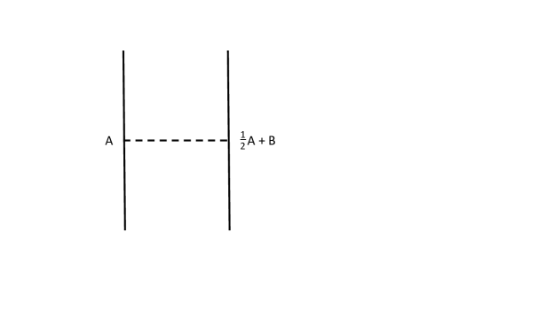
Figure 1: Contact terms in the toy model are generated by diagrams with exchange of $\phi$ (dashed). In gravity, with non-minimal term $\sim\int\!\sqrt{-g}F\left(\phi\right)R$ and matter field Lagrangian $\sim\int\!\sqrt{-g}L\left(\phi\right)$ then $A$ is replaced by $F(\phi)$ and $B$ is replaced by $L(\phi)$, and the dashed line is a graviton propagator.

We thus see that we have diagrammatically obtained a local effective action:

$$S=\int\frac{1}{2}\partial\phi\partial\phi+\frac{1}{2}A\partial^{2}A+AB+\makebox{ {long distance}}$$ (7)

Of course, we can see this straightforwardly by “solving the theory,” by defining a shifted field:

$$\phi=\phi^{\prime}-\frac{1}{\partial^{2}}\left(\partial^{2}A+B\right)$$ (8)

Substituting this into the action $S$ and integrating by parts yields:

$$S=\int\frac{1}{2}\partial\phi^{\prime}\partial\phi^{\prime}+\frac{1}{2}A\partial^{2}A+AB+\frac{1}{2}B\frac{1}{\partial^{2}}B$$ (9)

An equivalent effective local action that describes both short and large distance is then,

$$S=\int\frac{1}{2}\partial\phi\partial\phi+\frac{1}{2}A\partial^{2}A+AB-{B\phi}$$ (10)

The contact terms have become pointlike components of the effective action, while the remaining long distance effects are produced by the usual massless $\phi$ exchange. Note that the derivatively coupled operator $A$ has no long distance interactions due to $\phi$ exchange. Moreover, in the effective action of eq.(10) we have implicitly “integrated out” the $A\partial^{2}\phi$, which is no longer part of the action and is replaced by new operators $\frac{1}{2}A\partial^{2}A+AB$. We will see that this is exactly what happens with gravity, where the $A\partial^{2}\phi$ term is schematically the nonminimal $F(\phi)R(g)\sim F(\phi)\partial^{2}h$ term in a weak field expansion of gravity $g=\eta+h$.

One can also adapt the use of equations of motion to obtain eq.(10) from the action eq.(5) but this requires care. For example, the insertion of the $\phi$ equation of motion, into $A\partial^{2}\phi$ correctly gives the $AB$ term but misses the factor of $1/2$ in the $A\partial^{2}A$ term. We can therefore do a trick of defining a “modified equation of motion,” where we supply a factor of $1/2$ on the term $A\partial^{2}A$, e.g. substitute:

$$\partial^{2}\phi=-\partial^{2}A-B\rightarrow-\frac{1}{2}\partial^{2}A-B$$ (11)

in place of the $\partial^{2}\phi$ in the second term of eq.((5)) to obtain eq.(10).

IV Gravitational Contact Terms

Consider a general theory involving scalar fields $\phi_{i},$ an Einstein-Hilbert term and a non-minimal interaction:

$$\!\!\!\!\!\!\!\!\!\!\;\;S=\int\sqrt{-g}\left(\frac{1}{2}M^{2}R\left(g_{\mu\nu}\right)+\frac{1}{2}F\left(\phi_{i}\right)R\left(g_{\mu\nu}\right)+L\left(\phi_{i}\right)\right)$$

$$=S_{1}+S_{2}+S_{3}$$ (12)

where we use the metric signature and curvature tensor conventions of CCJ . $S_{1}$ is the kinetic term of gravitons

$$S_{1} = \frac{1}{2}M^{2}\int\sqrt{-g}R$$ (13)

and becomes the Fierz-Pauli action in a weak field expansion.

$S_{2}$ is the non-minimal interaction, and takes the form:

$$S_{2}=\frac{1}{2}\int\sqrt{-g}F\left(\phi_{i}\right)R\left(g_{\mu\nu}\right)$$ (14)

$S_{3}$ is the matter action with couplings to the gravitational weak field:

$$S_{3}=\int\sqrt{-g}\;L\left(\phi_{i}\right)$$ (15)

The Lagrangian takes the form

$$L\left(\phi_{i}\right)=\frac{1}{2}g^{\mu\nu}\partial_{\mu}\phi_{i}\partial_{\nu}\phi_{i}-W(\phi_{i})$$ (16)

with potential $W(\phi_{i})$. The matter lagrangian has stress tensor and stress tensor trace:

$$T_{\mu\nu} = \partial_{\mu}\phi_{i}\partial_{\nu}\phi_{i}-g_{\mu\nu}\left(\frac{1}{2}g^{\rho\sigma}\partial_{\rho}\phi_{i}\partial_{\sigma}\phi_{i}-W(\phi_{i})\right).$$

$$T = -\partial^{\sigma}\phi_{i}\partial_{\sigma}\phi_{i}+4W(\phi_{i})$$ (17)

There are then three ways to obtain the contact term:

(1) GRAVITON EXCHANGE CONTACT TERM

In reference HillRoss the corresponding Feynman diagrams of Figure 1 with are evaluated arising from single graviton exchange between the interaction terms.

We treat the theory perturbatively, expanding around flat space. Hence we linearize gravity with a weak field $h_{\mu\upsilon}$:

$$g_{\mu\upsilon}\approx\eta_{\mu\upsilon}+\frac{h_{\mu\upsilon}}{M}.$$ (18)

The scalar curvature is then:

$$R = R_{1}+R_{2}$$

$$MR_{1} = \biggl{(}\partial^{2}h\ -\partial^{\mu}\partial^{\nu}h_{\mu\nu}\biggr{)}$$

$$M^{2}R_{2} = -\frac{3}{4}\partial^{\rho}h^{\mu\nu}\partial_{\rho}h_{\mu\nu}-\frac{1}{2}h^{\mu\nu}\partial^{2}h_{\mu\nu}+...$$ (19)

(see HillRoss for the complete expression for $R_{2}$). $S_{1}$ then becomes:

$$S_{1}=\frac{1}{2}M^{2}\int\sqrt{-g}R=\frac{1}{2}M^{2}\int\!\!\left(R_{1}+R_{2}+\frac{1}{2}\frac{h}{M}R_{1}\right)$$

$$=\frac{1}{2}\int h^{\mu\nu}\biggl{(}\frac{1}{4}\partial^{2}\eta_{\mu\nu}\eta_{\rho\sigma}-\frac{1}{4}\partial^{2}\eta_{\mu\rho}\eta_{\nu\sigma}$$

$$\qquad\qquad-\frac{1}{2}\partial_{\rho}\partial_{\sigma}\eta_{\mu\nu}+\frac{1}{2}\partial_{\mu}\partial_{\rho}\eta_{\nu\sigma}\biggr{)}h^{\rho\sigma}.$$ (20)

Note that the leading term, $\int R_{1}$, is a total divergence and is therefore zero in the Einstein-Hilbert action, and what remains of eq.(IV) is the Fierz-Pauli action. This is key to the origin of the contact terms. The non-minimal interaction, $S_{2}$, then takes the leading form:

$$S_{2}=\frac{1}{2}\int\!\!\sqrt{-g}\;F\left(\phi\right)R\left(g\right)\rightarrow\frac{1}{2}\int\!\!F\left(\phi\right)R_{1}\left(g\right)$$

$$\qquad=\int\frac{1}{2M}F\left(\phi\right)\Pi^{\mu\nu}h_{\mu\nu}$$ (21)

where it is useful to introduce the transverse derivative,

$$\Pi^{\mu\nu}=\partial^{2}\eta^{\mu\nu}\ -\partial^{\mu}\partial^{\nu}.$$ (22)

$S_{2}$ involves derivatives, and is the analogue of the $A\partial^{2}\phi$ term in eq.(5). It will therefore generate contact terms in the gravitational potential due to single graviton exchange. $S_{3}$ is the analogue of the $B\phi$ term in eq.(5), and this situation will closely parallel the toy model.

In HillRoss we developed the graviton propagator, following the nice lecture notes of Donoghue et. al., Donoghue . We remark that we found a particularly useful gauge choice,

$$\partial_{\mu}h^{\mu\nu}=w\partial^{\nu}h$$ (23)

where $w$ defines a single parameter family of gauges. The familiar De Donder gauge corresponds to $w=\frac{1}{2}$, while the choice $w=\frac{1}{4}$ is particularly natural in this application, and the gauge invariance of the result is verified by the $w$-independence (we verify the Newtonian potential from graviton exchange between static masses in $w$ gauge; see HillRoss ).

We can the compute single graviton exchange between the interaction terms of the theory. A diagram with a single $S_{2}$ vertex and single $S_{3}$ vertex is the analogue of $AB$ in the toy model and yields:

$$-i\left\langle T\;S_{2}S_{3}\right\rangle=\int d^{4}x\;\frac{F\left(\phi_{i}\right)}{2M^{2}}T(\phi_{i})$$ (24)

Also we have the pair $\left\langle S_{2}S_{2}\right\rangle$ which corresponds to $\frac{1}{2}A\partial^{2}A$ in the toy model and yields:

$$-i{\left\langle T\;S_{2}S_{2}\right\rangle} = -\int d^{4}x\;\frac{3}{4M^{2}}\;F\left(\phi_{i}\right)\!\partial^{2}F\left(\phi_{i}\right)$$

Hence, the action becomes

$$S=S_{1}+S_{3}+S_{CT}$$ (26)

where

$$S_{CT}=\int d^{4}x\biggl{(}-\frac{3}{4M^{2}}F\partial^{2}F+\frac{1}{2M^{2}}FT\biggr{)}$$ (27)

Note the sign of the $F\partial^{2}F$ is opposite (repulsive) to that of the toy model $A\partial^{2}A$. Since this is a tree diagram effect, it is classical.

(2) WEYL TRANSFORMATION

In eq.(IV) we define:

$$\Omega^{2}=\left(1+\frac{F\left(\phi_{i}\right)}{M^{2}}\right)$$ (28)

and perform a Weyl transformation on the metric:

$$g_{\mu\nu}(x)\rightarrow\Omega^{-2}g_{\mu\nu}(x)\qquad g^{\mu\nu}(x)\rightarrow\Omega^{2}g^{\mu\nu}(x)$$

$$\sqrt{-g}\rightarrow\sqrt{-g}\Omega^{-4}$$

$$R(g)\rightarrow\Omega^{2}R(g^{\prime})+6\Omega^{3}D\partial\Omega^{-1}$$ (29)

and the action of eq.(V) becomes:

$$S\rightarrow\int\sqrt{-g}\biggl{(}\frac{1}{2}M^{2}R\left(g\right)$$

$$-3M^{2}\partial_{\mu}\left(1+\frac{F}{M^{2}}\right)^{1/2}\!\!\partial^{\mu}\left(1+\frac{F}{M^{2}}\right)^{-1/2}$$

$$+\frac{1}{2}\left(1+\frac{F}{M^{2}}\right)^{-1}\!\!\!\partial_{\mu}\phi_{i}\partial^{\nu}\phi^{i}-\left(1+\frac{F}{M^{2}}\right)^{-2}\!\!\!W(\phi_{i})\biggr{)}$$

Keeping terms to $O({1\over M^{2}})$ and integrating by parts we have:

$$\!\!\!\!\!\!\!\!\!\!S=S_{1}+S_{3}$$

$$\!\!\!\!\!\!\!\!\!\!+\int d^{4}x\bigg{(}-\frac{3F\left(\phi_{i}\right)\partial^{2}F\left(\phi_{i}\right)}{4M^{2}}+\frac{F\left(\phi_{i}\right)T\left(\phi_{i}\right)}{2M^{2}}\bigg{)}$$ (31)

The Weyl transformed action is identically consistent with the contact terms of eq.(27) above, to first order in $1/M^{2}$.

Hence, contact terms arise in gravity with non-minimal couplings to scalar fields due to graviton exchange and their form is equivalent to a Weyl redefinition of the theory to the Einstein frame. However we emphasie that the contact terms are not a Weyl tranformation since they do not involve a rescaling of the metric, and there would therefore be no Jacobian ghost terms introduced into the path integral. Hence any theory with a non-minimal interaction $\sim F(\phi)R$ will lead to contact terms at order $1/M^{2}$. What we say presently only applies on scales below $M$, hence the Jordan frame would, at best, apply only in a UV completion of the theory to pre-Planckian scales.

(3) USE OF $R$ (MODIFIED) EQUATION OF MOTION

The Einstein equation with the nonminimal term is:

$$M^{2}G_{\alpha\beta}=-T_{\alpha\beta}-D_{\mu}(D_{\nu}F(\phi_{i}))+g_{\mu\nu}D^{2}F(\phi_{i})$$

$$M^{2}R=T-3D^{2}F(\phi_{i})$$ (32)

We can use a simple trick to obtain the contact term via a modified the equation of motion for $R$. We supply a factor of $1/2$ in the last term which is the analogue of the $\partial^{2}A$ term as in eq.(11):

$$R^{\prime}=\frac{1}{M^{2}}\biggl{(}T-\frac{3}{2}D^{2}F(\phi_{i})\biggr{)}$$ (33)

Then substitute $R^{\prime}$ for $R$ in the non-minimal term $FR$ of the action of eq.(V)

$$\!\!\!\!\!\!\!\!\!\!\;\;S\rightarrow\int\sqrt{-g}\left(\frac{1}{2}M^{2}R\left(g_{\mu\nu}\right)+\frac{1}{2}F\left(\phi_{i}\right)R^{\prime}\left(g_{\mu\nu}\right)+L\left(\phi_{i}\right)\right)$$

$$\qquad=S_{1}+S_{3}$$

$$\qquad+\int d^{4}x\bigg{(}-\frac{3F\left(\phi_{i}\right)\partial^{2}F\left(\phi_{i}\right)}{4M^{2}}+\frac{F\left(\phi_{i}\right)T\left(\phi_{i}\right)}{2M^{2}}\bigg{)}$$

In the RG calculation we will only need the exact equation of motion for $R$ in the Einstein frame (without the pseudo $-3D^{2}F/2$ term), so this ambiguity does not arise.

V Effective Potetial in a Simple Model

Consider the following action:

$$\!\!\!\!\!\!\!\!\!\!S_{Jordan}=\int\sqrt{-g}\biggl{(}\frac{1}{2}\partial\phi\partial\phi-\frac{\lambda_{1}}{4}\phi^{4}-\frac{\lambda_{2}\phi^{6}}{12M^{2}}$$

$$-\frac{\gamma}{12}\frac{\phi^{2}}{M^{2}}\partial\phi\partial\phi-\frac{\alpha}{12}\phi^{2}R+\frac{1}{2}M^{2}R\biggr{)}$$ (35)

This is the most general action for a real scalar field with a $Z_{2}$ symmetry $\phi\rightarrow-\phi$ valid to O($M^{-2}$) with Einstein gravity and assuming $\phi$ is massless, $m^{2}=0$. Here we do not include a term $\phi^{4}R/M^{2}$ since, after use of equations of motion, $R\sim M^{-2}$ such a term would enter the physics at O($M^{-4}$).

We can go to the Einstein frame by implementing the CT. We find that the effect of single graviton exchange to eq.(V) yields a new action to order $M^{-2}$:

$$\!\!\!\!\!\!\!\!\!\!S_{Einstein}=\!\int\!\sqrt{-g}\biggl{(}\frac{1}{2}\partial\phi\partial\phi-\frac{\lambda^{\prime}_{1}}{4}\phi^{4}-\frac{\lambda^{\prime}_{2}\phi^{6}}{12M^{2}}$$

$$-\frac{\gamma^{\prime}\phi^{2}}{12M^{2}}\partial\phi\partial\phi+\frac{1}{2}M^{2}R\biggr{)}$$ (36)

where:

$$\gamma^{\prime}=\gamma-\alpha-\alpha^{2}$$

$$\lambda_{1}^{\prime}=\lambda_{1}$$

$$\lambda_{2}^{\prime}=\lambda_{2}+\alpha\lambda_{1}$$ (37)

We see that to first order in $M^{-2}$ in $S_{Einstein}$ we have three interaction terms, though the original action $S_{Jordan}$ displayed four interaction terms. In the Einstein frame action we see that $\alpha$ has disappeared having been absorbed into redefining the other coupling constants. This indicates that the nonminimal term in $S_{Jordan}$ with coupling $\alpha$ is unphysical. Moreover, if we are careful to incorporate the effects of the contact term, then $S_{Einstein}$ will “close” under renormalization.

We define,

$$Z=1-\frac{\gamma^{\prime}\phi^{2}}{6M^{2}}$$ (38)

and the Einstein action becomes:

$$S_{Einstein}=\!\int\!\sqrt{-g}\biggl{(}\frac{1}{2}Z\partial\phi\partial\phi-\frac{\lambda^{\prime}_{1}}{4}\phi^{4}-\frac{\lambda^{\prime}_{2}\phi^{6}}{12M^{2}}$$

$$+\frac{1}{2}M^{2}R\biggr{)}$$ (39)

We do a background field calculation where we shift $\phi\rightarrow\phi_{0}+\sqrt{\hbar}Z_{0}^{-1/2}\hat{\phi}$, where we define

$$Z_{0}=1-\frac{\gamma^{\prime}\phi_{0}^{2}}{6M^{2}}$$ (40)

We will treat $\phi\rightarrow\phi_{0}$ as a constant and compute the one loop, $\cal{O(\hbar)}$ effective potential in $\phi_{0}$ integrating out the quantum fluctuations $\hat{\phi}$ . Expand the action with the shifted field to O$(\hat{\phi}^{2})$, dropping terms odd in $\hat{\phi}$ for constant $\phi_{0}$.

$$\!\!\!\!\!\!\!\!\!\!S_{Einstein}=$$

$$\!\!\!\!\!\!\!\!\!\!\int\sqrt{-g}\biggl{(}\frac{1}{2}\partial\hat{\phi}\partial\hat{\phi}-\frac{1}{2}B\hat{\phi}^{2}-V_{0}(\phi_{0})+\frac{1}{2}M^{2}R\biggr{)}$$

where,

$$Z_{0}=1-\frac{\gamma^{\prime}\phi_{0}^{2}}{6M^{2}}$$

$$B=Z_{0}^{-1}\biggl{(}{3\lambda^{\prime}_{1}}\phi_{0}^{2}+\frac{5\lambda^{\prime}_{2}}{2M^{2}}\phi_{0}^{4}\biggr{)}$$

$$={3\lambda^{\prime}_{1}}\phi_{0}^{2}+\frac{5\lambda^{\prime}_{2}+\gamma^{\prime}\lambda^{\prime}_{1}}{2M^{2}}\phi_{0}^{4}$$

$$V_{0}(\phi_{0})=\frac{\lambda^{\prime}_{1}}{4}\phi_{0}^{4}+\frac{\lambda^{\prime}_{2}}{12}\frac{\phi_{0}^{6}}{M^{2}}$$

First we consider the non-curvature terms, with flat Minkowsky space metric $g_{\mu\nu}=\eta_{\mu\nu}$. We obtain the effective potential from the log of the path integral described briefly in the Appendix, eq.(71), obtained by integrating out $\hat{\phi}^{2}$. Presently we plug $m^{2}\rightarrow B$ into the path integral expression of eq.(71),

$$\Gamma_{0} = -\frac{1}{2}B^{2}L+O\biggl{(}\frac{B^{3}}{\Lambda^{2}}\biggr{)}$$ (43)

and we define the log as:

$$L=\frac{1}{16\pi^{2}}\ln\frac{\Lambda}{\mu}$$ (44)

with a generic infrared cut-off mass scale $\mu$. Hence, squaring $B$ to O($\hbar$), the resulting potential is to ${\cal{O}}(\phi_{0}^{6})$:

$$\!\!\!\!\!\!\!\!\!\!\!\!\Gamma_{0}=-\biggl{(}\frac{9\lambda^{\prime 2}_{1}}{2}\phi_{0}^{4}+\frac{(15\lambda^{\prime}_{2}\lambda^{\prime}_{1}+3\gamma^{\prime}\lambda^{\prime}_{1}{}^{2})}{2}\frac{\phi_{0}^{6}}{M^{2}}\biggr{)}L$$ (45)

Note that $\mu\rightarrow\phi_{0}$ in the logarithm this is essentialy a Coleman-Weinberg potential CW .

V.1 Inclusion of Gravitational Effects

Consider the weak field approximation to gravity. We choose $w$-gauge of eq.(23) and obtain

$$\partial_{\alpha}h^{\alpha\beta}=w\partial^{\beta}h,\qquad R=(1-w)\partial^{2}h/M$$ (46)

Up to linear terms in $h_{\mu\nu}\hat{\phi}^{2}/M$ we have,

$$S_{Einstein}\rightarrow\int\Biggl{(}\frac{1}{2}\partial_{\mu}\hat{\phi}\partial^{\mu}\hat{\phi}+\frac{1}{4}\frac{h}{M}\partial_{\mu}\hat{\phi}\partial^{\mu}\hat{\phi}+\frac{1}{2}M^{2}R$$

$$-\frac{h^{\mu\upsilon}}{2M}\partial_{\mu}\hat{\phi}\partial_{\nu}\hat{\phi}-\frac{1}{2}\biggl{(}1+\frac{1}{2}\frac{h}{M}\biggr{)}B\hat{\phi}^{2}-V_{0}(\phi_{0})\Biggr{)}$$ (47)

The contributions to the potential from the Feynman diagrams of Figs.(1,2) are then,

$$\!\!\!\!\!\!\!\!\!\!\!\!\!\!\!\!\!\!\!\!\Gamma_{D1}=-\frac{\bigl{(}1+2w\bigr{)}}{12M}B\partial^{2}hL$$

$$\!\!\!\!\!\!\!\!\!\!\!\!\!\!\!\!\!\!\!\!\Gamma_{D2}=\frac{B}{4M}\partial^{2}hL$$ (48)

Full details will be given in Ghil . Noting that,

$$\frac{1}{4M}\partial^{2}h-\frac{(1+2w)}{12M}\partial^{2}h=\frac{(1-w)}{6M}\partial^{2}h=\frac{1}{6M}R$$

Hence we have the net contribution to the potential,

$$\Gamma_{\alpha}\equiv\Gamma_{D1}+\Gamma_{D2}=\frac{1}{6}BR\;L=\frac{\lambda_{1}\phi_{0}^{2}}{2}RL$$ (50)

We thus see that there is a $\delta\alpha\phi_{0}^{2}R/12$ term generated from the $3\lambda^{\prime}_{1}\phi_{0}^{2}$ term in B:

$$\delta\alpha=6\lambda^{\prime}_{1}L+O(1/M^{2})$$ (51)

Note that there are other terms proportional to $R$, but we only keep leading terms in $1/M^{2}$ in $\delta\alpha$, since $R\sim 1/M^{2}$.

To implement the contact term we use, in eq.(50), the leading order $R$ equation of motion in the Einstein frame,

$$R=\frac{1}{M^{2}}T=\frac{1}{M^{2}}4\times\biggl{(}\frac{\lambda_{1}}{4}\phi_{0}^{4}-\frac{9\lambda^{2}_{1}}{2}\phi_{0}^{4}L\biggr{)}+{\cal{O}}\biggl{(}\frac{1}{M^{4}}\biggr{)}$$

$$\rightarrow\lambda_{1}\frac{\phi_{0}^{4}}{M^{2}}+{\cal{O}}(\hbar)$$ (52)

We then have

$$\Gamma_{\alpha}=\frac{1}{2}\lambda^{\prime}_{1}\phi^{2}_{0}R\;L\rightarrow\frac{\lambda^{\prime 2}_{1}\phi_{0}^{6}}{2M^{2}}L+{\cal{O}}\frac{1}{M^{4}}$$ (53)

Therefore, combining all effects

$$\Gamma_{Einstein}\equiv V_{0}+\Gamma_{0}+\Gamma_{\alpha}=$$

$$\frac{\lambda_{1}}{4}\phi_{0}^{4}+\frac{\lambda_{2}}{12}\frac{\phi_{0}^{6}}{M^{2}}$$

$$-\frac{1}{2}\biggl{(}9\lambda^{2}_{1}\phi_{0}^{4}+(15{\lambda_{1}\lambda_{2}}+3\lambda^{2}_{1}\gamma-[\lambda_{1}^{2}])\frac{\phi_{0}^{6}}{M^{2}}\biggr{)}L$$ (54)

where the term in $[..]$ comes from the gravitational effects of D1 and D2.

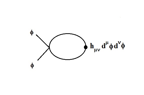
Figure 2: Diagram D1.

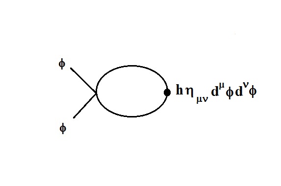
Figure 3: Diagram D2.

From eq.(V.1) we can extract the $\beta$-functions for $\lambda_{1}$ and $\lambda_{2}$. Define $D=16\pi^{2}\partial/\partial\ln\mu$, and we have:

$$D\lambda_{1}=18\lambda_{1}^{2}$$

$$D\lambda_{2}=90\lambda_{1}\lambda_{2}-6\lambda_{1}^{2}+18\lambda^{2}\gamma^{\prime}$$ (55)

In Ghil we obtain the RG equation for $\gamma^{\prime}$, but this requires an effective action for non-constant $\phi_{0}$.

V.2 Comparison to a Conventional Calculation of $\beta_{\alpha}$
in Jordan Frame Neglecting Contact Terms

We now compute the potential in the Jordan frame where we neglect the contact term, as is conventionally done. Here we again use the background field method.

Return to $S_{Jordan}$, and begin by shifting $\phi\rightarrow\phi_{0}+\sqrt{\hbar}\hat{\phi}$ and expanding to O$\hat{\phi}^{2}$ where $\phi_{0}$ is a constant classical background field and $\sqrt{\hbar}\hat{\phi}$ is a quantum fluctuation. Henceforth we will suppress the factor of $\sqrt{\hbar}$ but we will compute loops to order $\hbar$. The shifted action where we drop the linear terms in $\hat{\phi}$ becomes to order $\hbar$:

$$S_{Jordan}=\int\sqrt{-g}\biggl{(}\frac{1}{2}g^{\mu\upsilon}\partial_{\mu}\hat{\phi}\partial_{\nu}\hat{\phi}$$

$$-\frac{1}{2}Z_{0}^{-1}A\hat{\phi}^{2}R-\frac{1}{2}B\hat{\phi}^{2}-V_{0}(\phi_{0})+\frac{1}{2}M^{2}R\biggr{)}$$ (56)

where, we have the relations of eq.(V), but with unprimed couplings replacing the primed ones, and

$$A=\frac{\alpha}{6}$$ (57)

Expanding to linear terms in $h_{\mu\nu}/M$ in weak field gravity the action eq.(V.2) becomes

$$S\rightarrow\int\Biggl{(}\frac{1}{2}\partial_{\mu}\hat{\phi}\partial^{\mu}\hat{\phi}+\frac{h}{4M}\eta^{\mu\nu}\partial_{\mu}\hat{\phi}\partial_{\nu}\hat{\phi}-\frac{h^{\mu\upsilon}}{2M}\partial_{\mu}\hat{\phi}\partial_{\nu}\hat{\phi}$$

$$-\frac{1}{2}Z_{0}^{-1}AR{\hat{\phi}^{2}}-\frac{1}{2}B\hat{\phi}^{2}-B\frac{h}{4M}\hat{\phi}^{2}-V_{0}(\phi_{0})+\frac{1}{2}M^{2}R\Biggr{)}$$

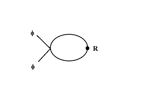
Figure 4: Diagram D2.

Neglecting the contact terms we see, in addition to the non-curvature potential obtained previously in eq.(45), the action eq.(V.2) now (naively) generates three diagrams linear in the curvature, D1, D2, and D3 of Figs(2,3,4). The additional D3 diagram (which is absent in the Einsteain frame) is:

$$\!\!\!\!\!\!\!\!\!\!\!\!\!\!\!\!\!\!\!\!\Gamma_{D3}=-Z_{0}^{-1}ABRL=-\frac{\alpha}{6}BRL+O\frac{1}{M^{2}}R$$ (59)

Hence we have from eqs.(50,59) for (D1+D2+D3):

$$\Gamma_{D3}+\Gamma_{\alpha}=-\frac{1}{6}(\alpha-1)BR\;L$$

$$=-\frac{1}{6}(\alpha-1)\biggl{(}{3\lambda_{1}}\phi_{0}^{2}+\frac{5\lambda_{2}+\gamma\lambda_{1}}{2M^{2}}\phi_{0}^{4}\biggr{)}RL$$ (60)

Therefore, combining all effects:

$$\Gamma_{Jordan}=$$

$$\frac{\lambda_{1}}{4}\phi_{0}^{4}+\frac{\lambda_{2}}{12}\frac{\phi_{0}^{6}}{M^{2}}+\frac{\alpha}{12}\phi_{0}^{2}R+\frac{\gamma}{12M^{2}}\phi_{0}^{2}R$$

$$-\frac{1}{2}L\biggl{(}9\lambda^{2}_{1}\phi_{0}^{4}+(15{\lambda_{1}\lambda_{2}}+3\lambda^{2}_{1}\gamma)\frac{\phi_{0}^{6}}{M^{2}}\biggr{)}$$

$$-\frac{1}{6}(\alpha-1)\biggl{(}{3\lambda_{1}}\phi_{0}^{2}+\frac{5\lambda_{2}+\gamma\lambda_{1}}{2M^{2}}\phi_{0}^{4}\biggr{)}RL$$ (61)

This contains the conventional radiative correction and renormaliztion group running of $\alpha$

$$\alpha\rightarrow\alpha+6\lambda_{1}(1-\alpha)L$$ (62)

We again use the leading order $R$ equation of motion in the Einstein frame as in eq.(V.1) to implement the contact term, but must now keep the $\lambda^{2}_{1}L$ term,

$$R\rightarrow(\lambda_{1}-18\lambda^{2}_{1}L)\frac{\phi_{0}^{4}}{M^{2}}+{\cal{O}}(\hbar)$$ (63)

hence

$$\Gamma_{Jordan}\equiv V_{0}+\Gamma_{0}+\Gamma_{\alpha}+\Gamma_{D3}$$

$$=\frac{\lambda_{1}}{4}\phi_{0}^{4}+\frac{\lambda_{2}+\alpha\lambda_{1}}{12}\frac{\phi_{0}^{6}}{M^{2}}-\frac{2\lambda^{2}_{1}\alpha\phi_{0}^{6}}{M^{2}}L$$

$$-\frac{1}{2}L\biggl{(}9\lambda^{2}_{1}\phi_{0}^{4}+(15{\lambda_{1}\lambda_{2}}+3\lambda^{2}_{1}\gamma-[\lambda_{1}^{2}])\frac{\phi_{0}^{6}}{M^{2}}\biggr{)}$$

$$=$$

$$\frac{\lambda^{\prime}_{1}}{4}\phi_{0}^{4}+\frac{\lambda^{\prime}_{2}}{12}\frac{\phi_{0}^{6}}{M^{2}}+\frac{\lambda^{\prime 2}_{1}\alpha\phi_{0}^{6}}{2M^{2}}L\biggl{(}8-{3}\alpha\biggr{)}$$

$$-\frac{1}{2}L\biggl{(}9\lambda^{\prime 2}_{1}\phi_{0}^{4}+(15{\lambda^{\prime}_{1}\lambda^{\prime}_{2}}+3\lambda^{\prime 2}_{1}\gamma^{\prime}-[\lambda^{\prime}_{1}{}^{2}])\frac{\phi_{0}^{6}}{M^{2}}\biggr{)}$$

where we’ve converted to the Einstein frame primed variables via eqs.(V). Comparing to eq.(V.1) we therefore see an inconsistency between the potentials $\Gamma_{Einstein}$ and $\Gamma_{Jordan}$ at O($\hbar$):

$$\!\!\!\!\!\!\!\!\!\!\Gamma_{Einstein}-\Gamma_{Jordan}=\frac{(8-3\alpha)\alpha\lambda^{\prime 2}_{1}\phi_{0}^{6}}{2M^{2}}\hbar L$$ (65)

The fault lies in the Jordan frame calculation which does not implement the contact term.

One might attempt to interpret this as a quantum “frame anomaly.” We see some vague parallels with the axial anomaly here, but we think the issue is more of an error that one is making in computing naively. Such an anomaly interpretation would require identifying an operator that plays a special roll in the Weyl tranformation and that has matrix elements given by the rhs of eq,(65). Perhaps this can be related to the Weyl current, but we have not yet explored this possibility.

VI CONCLUSIONS

The Weyl transformation acting on the Jordan frame, to remove non-minimal interactions leading to the minimal Einstein frame, is identical to implementing the contact terms HillRoss . If one didn’t know about the Weyl transformation one would discover it in the induced contact terms in the single graviton exchange potential involving non-minimal couplings. The Weyl transformation is powerful as it is fully non-perturbative. Technically it can provide a useful check on the normalization and implementation of the graviton propagators in various gauges. But the contact term stipulates that the mapping to the Einstein frame is dynamical and inevitable, and does not involve field redefinitions.

In a model with non-minimal coupling $-\alpha\phi^{2}R/12$ this implies that the parameter $\alpha$ doesn’t really exist physically. Computing $\beta$-functions in a Jordan frame without implementing the contact term will yield incorrect results. Implementing the contact term yields the Einstein frame and results computed there will have no contact term ambiguities.

However, the Einstein frame has a loop induced contact term which is then absorbed back into the potential terms by the contact terms (equivalently, a mini-Weyl transformation, or use of the $R$ equation of motion). The use of the $R$ equation of motion on the non-minimal term is analogous to the use of the gluon field equation for the electroweak penguin. It is likely the Deans and Dixon Deans constraints on null operators applies to gravity as well. This implies generally that there are pitfalls in directly interpreting any physics in the Jordan frame.

We emphasize that our analysis applies strictly to a theory with a Planck mass term. A Weyl invariant theory, where $M=0$, is nonperturbative and our analysis is then inapplicable, and the Jordan frame may then be physically relevant. Indeed, there is no conventional gravity in this limit since the usual $M^{2}R$ (Fierz-Pauli) graviton kinetic term does not then exist. Hence in this limit one would have to appeal to a UV completion, e.g., string theory or $R^{2}$ gravity, etc.

In the case of an $R^{2}$ UV completion theory we view the formation of the Planck mass by, e.g., inertial symmetry breaking, i.e., as a dynamical phase transition, similar to a disorder-order phase transition in a material medium FHR . An intriguing point to note is that if we have an $R^{2}$ UV completion, then the graviton propagator is $\propto 1/q^{4}$. But then the $AR\sim Ahq^{2}$ vertex implies a $1/q^{2}$ graviton exchange amplitude, which means an inverse square law “pseudo-gravitational force” exists even above the Planck scale to fields that couple non-minimally. This is remarkable to us and one of many issues to develop further in this context.

Acknowledgements

Part of this work was done at Fermilab, operated by Fermi Research Alliance, LLC under Contract No. DE-AC02-07CH11359 with the United States Department of Energy.

Appendix A Projection-Regulated Feynman Loops

The loop induced effective potential for $\phi_{0}$ provides a useful way to extract all of the $\beta$-functions of the various coupling constants. The potential $\Gamma(\phi_{0})$ is the log of the path integral: $\Gamma=i\ln P$. In the case of a real scalar field with mass term we consider the free action,

$$\frac{1}{2}\int d^{4}x\biggl{(}\partial\phi\partial\phi-m^{2}\phi^{2}\biggr{)}$$ (66)

we have for the path integral:

$$P=\underset{k}{\prod}\biggl{(}k^{2}-m^{2}\biggr{)}^{-1/2}=\det\biggl{(}k^{2}-m^{2}\biggr{)}^{-1/2}$$ (67)

whre $k=(k_{0},\vec{k})$ is the $4$-momentum hence, we have:

$$\Gamma=i\ln P=-\frac{i}{2}\int\frac{d^{4}k}{(2\pi)^{4}}\ln\biggl{(}k^{2}-m^{2}+i\epsilon\biggr{)}$$ (68)

This can be evaluated with a Wick rotation to a Euclidean momentum, $k\rightarrow k_{E}=(ik_{0},\vec{k})$, and a Euclidean momentum space cut off $\Lambda$:

$$\Gamma = \frac{1}{2}\int_{0}^{\Lambda}\frac{d^{4}k_{E}}{(2\pi)^{4}}\ln\biggl{(}\frac{k_{E}^{2}+m^{2}}{\Lambda^{2}}\biggr{)}$$ (69)

$$\!\!\!\!\!\!\!\!\!\!=\frac{1}{64\pi^{2}}\biggl{(}\Lambda^{4}\ln\frac{\Lambda^{2}+m^{2}}{\Lambda^{2}}-m^{4}\ln\frac{\Lambda^{2}+m^{2}}{m^{2}}$$

$$\!\!\!\!\!\!\!\!\!\!\!\!\!\!\!\!\!\!\!\!\qquad-\frac{1}{2}\Lambda^{4}+\Lambda^{2}m^{2}\biggr{)}+(\makebox{irrelevant constants})$$

The cutoff can be viewed is a spurious parameter, introduced to make the integral finite and arguments of logs dimensionless, but and not part of the defining action. The only physically meaningful dependence upon $\Lambda$ is contained in the logarithm, where it reflects scale symmetry breaking by the quantum trace anomaly. Powers of $\Lambda$, e.g., $\Lambda^{4},\Lambda^{2}m^{2}$, spuriously break scale symmetry and are not part of the classical action Bardeen .

It is therefore conceptually useful to have a definition of the loops in which the spurious powers of $\Lambda$ do not arise. This can be done by defining the loops applying projection operators on the integrals. The projection operator

$$P_{n}=\biggl{(}1-\frac{\Lambda}{n}\frac{\partial}{\partial\Lambda}\biggr{)}$$ (70)

removes any terms proportional to $\Lambda^{n}.$ Since the defining classical Lagrangian has mass dimension 4 and involves no terms with $\Lambda^{2}m^{2}$ or $\Lambda^{4},$ we define the regularized loop integrals as:

$$\Gamma \rightarrow \frac{1}{2}P_{2}P_{4}\int_{0}^{\Lambda}\frac{d^{4}k_{E}}{(2\pi)^{4}}\ln\biggl{(}\frac{k_{E}^{2}+m^{2}}{\Lambda^{2}}\biggr{)}$$ (71)

$$= -\frac{1}{64\pi^{2}}m^{4}\biggl{(}\ln\frac{\Lambda^{2}}{m^{2}}\biggr{)}+O\biggl{(}\frac{m^{6}}{\Lambda^{2}}\biggr{)}$$

where we take the limit $\Lambda>>m$ to suppress $O(m^{6}/{\Lambda^{2}})$ terms and we are interested only in the log term (not additive constants) This means that the additive, non-log terms, e.g. $c^{\prime}m^{2}$, are undetermined, and the only physically meaningful result is the $\ln(\Lambda^{2}/m^{2})$ term. $\Lambda$ can be swapped for a renormalization scale $\mu$. Interestingly, if we define the integral as $\int\rightarrow P_{1}P_{2}P_{3}...P_{\infty}\int$, the action on the logs will lead to the Euler constant that arises in dimensional regularization, hinting at a mapping to the dimensionally regularized result.

References

- (1) C. T. Hill and G. G. Ross, Nucl. Phys. B 148, 373-399 (1979)
- (2) C. T. Hill and G. G. Ross, Nucl. Phys. B 171, 141-153 (1980); ibid., Phys. Lett. B 94, 234 (1980) doi:10.1016/0370-2693(80)90866-7
- (3) M. A. Shifman, A. I. Vainshtein and V. I. Zakharov, Nucl. Phys. B 120, 316-324 (1977).
- (4) J. R. Ellis, M. K. Gaillard, D. V. Nanopoulos and S. Rudaz, Nucl. Phys. B 131 (1977), 285 [erratum: Nucl. Phys. B 132 (1978), 541].
- (5) B. Pendleton and G. G. Ross, Phys. Lett. B 98, 291-294 (1981)
- (6) C. T. Hill, Phys. Rev. D 24, 691 (1981);
- (7) C. T. Hill and G. G. Ross, Phys. Lett. B 203, 125-131 (1988); ibid., Nucl. Phys. B 311, 253-297 (1988)
-
(8)
C. T. Hill, D. N. Schramm and J. N. Fry,
Comments Nucl. Part. Phys. 19, no.1, 25-39 (1989)
J. A. Frieman, C. T. Hill, A. Stebbins and I. Waga, Phys. Rev. Lett. 75, 2077-2080 (1995) -
(9)
Y. Nambu,
“Bootstrap Symmetry Breaking in Electroweak Interactions,”
EFI-89-08.
V. A. Miransky, M. Tanabashi and K. Yamawaki, Mod. Phys. Lett. A 4, 1043 (1989) - (10) W. A. Bardeen, C. T. Hill and M. Lindner, Phys. Rev. D 41, 1647 (1990)
- (11) C. T. Hill, “Naturally Self-Tuned Low Mass Composite Scalars,” [arXiv:2201.04478 [hep-ph]].
- (12) Hermann Weyl, Raum, Zeit, Materie (Space, Time, Matter), “Lectures on General Relativity,” (in German) Berlin, Springer (1921).
-
(13)
a partial list:
C. Brans and R. H. Dicke, Phys. Rev. 124, 925-935 (1961); S. W. Hawking, Commun. Math. Phys. 25, 167-171 (1972); Y. Fujii, Phys. Rev. D 9, 874-876 (1974);
G. W. Horndeski, Int. J. Theor. Phys. 10, 363-384 (1974);
K. A. Bronnikov, Acta Phys. Polon. B 4, 251-266 (1973);
M. Reuter and H. Weyer, Phys. Rev. D 69, 104022 (2004);
For a recent review of Weyl invariant theories, see: C. Wetterich, “Quantum scale symmetry,” [arXiv:1901.04741 [hep-th]],
A partial list of relevant papers to Weyl theories:
C. Wetterich, Nucl. Phys. B 302, 668 (1988);
M. Shaposhnikov and D. Zenhausern, Phys. Lett. B 671, 162 (2009);
D. Blas, M. Shaposhnikov and D. Zenhausern, Phys. Rev. D 84, 044001 (2011).
J. Garcia-Bellido, J. Rubio, M. Shaposhnikov and D. Zenhausern, Phys. Rev. D 84, 123504 (2011).
I. Quiros, arXiv:1405.6668 [gr-qc]; arXiv:1401.2643 [gr-qc];
A. Strumia, JHEP 1505, 065 (2015)
P. G. Ferreira, C. T. Hill and G. G. Ross, Phys. Lett. B 763, 174-178 (2016)
G. K. Karananas and J. Rubio, Phys. Lett. B 761, 223-228 (2016)
D. M. Ghilencea, Phys. Rev. D 93, no. 10, 105006 (2016); arXiv:1605.05632 [hep-ph].
D. M. Ghilencea, Z. Lalak and P. Olszewski, arXiv:1608.05336 [hep-th].
P. G. Ferreira, C. T. Hill and G. G. Ross, Phys. Rev. D 95, no.4, 043507 (2017)
K. Kannike, M. Raidal, C. Spethmann and H. Veermae, JHEP 1704 (2017) 026
A. Karam, T. Pappas and K. Tamvakis, Phys. Rev. D 96, no. 6, 064036 (2017);
J. Rubio and C. Wetterich, Phys. Rev. D 96, no. 6, 063509 (2017);
E. Guendelman, E. Nissimov and S. Pacheva, arXiv:1709.03786 [gr-qc];
J. Kubo, M. Lindner, K. Schmitz and M. Yamada, Phys. Rev. D 100, no.1, 015037 (2019)
T. Katsuragawa, S. Matsuzaki and E. Senaha, Chin. Phys. C 43, no.10, 105101 (2019)
D. Benisty and E. I. Guendelman, Class. Quant. Grav. 36, no.9, 095001 (2019)
D. M. Ghilencea and H. M. Lee, Phys. Rev. D 99, no.11, 115007 (2019)
D. M. Ghilencea, JHEP 10, 209 (2019); Phys. Rev. D 101, no.4, 045010 (2020). - (14) C. T. Hill and G. G. Ross, Phys. Rev. D 102, 125014 (2020).
- (15) C. T. Hill and G. G. Ross, Phys. Rev. D 104, no.2, 025002 (2021).
- (16) C. T. Hill and D. Ghilencea, work in progress, FERMILAB-PUB-22-645-T.
- (17) See, e.g., M. J. Duff and P. van Nieuwenhuizen, Phys. Lett. B 94, 179-182 (1980); M. J. Duff, “Inconsistency of Quantum Field Theory in Curved Space-time, ICTP/79-80/38; R. Jackiw, private communication.
- (18) M. S. Ruf and C. F. Steinwachs, Phys. Rev. D 97, no.4, 044050 (2018)
- (19) W. S. Deans and J. A. Dixon, Phys. Rev. D 18, 1113-1126 (1978); an explicit example is given in: C. T. Hill, Nucl. Phys. B 156, 417-426 (1979).
- (20) C. T. Hill, Phys. Rev. D 91, no.11, 111702 (2015); Phys. Rev. D 93, no.2, 025007 (2016); “Theorem: A Static Magnetic N-pole Becomes an Oscillating Electric N-pole in a Cosmic Axion Field,” [arXiv:1606.04957 [hep-ph]].
- (21) S. R. Coleman and E. J. Weinberg, Phys. Rev. D 7, 1888-1910 (1973) doi:10.1103/PhysRevD.7.1888
-
(22)
J. F. Donoghue,
“Introduction to the effective field theory description of gravity,”
[arXiv:gr-qc/9512024 [gr-qc]]; see also [arXiv:2009.00728 [hep-th]];
J. F. Donoghue, M. M. Ivanov and A. Shkerin, “EPFL Lectures on General Relativity as a Quantum Field Theory,” [arXiv:1702.00319 [hep-th]]. - (23) C. G. Callan, Jr., S. R. Coleman and R. Jackiw, Annals Phys. 59, 42-73 (1970).
- (24) P. G. Ferreira, C. T. Hill and G. G. Ross, Phys. Lett. B 763, 174 (2016). ibid Phys. Rev. D 95, no. 4, 043507 (2017); Phys. Rev. D 98, no.11, 116012 (2018); C. T. Hill, [arXiv:1803.06994 [hep-th]].
- (25) W. A. Bardeen, “On naturalness in the standard model,” FERMILAB-CONF-95-391-T.