Robust Locomotion on Legged Robots through Planning on
Motion Primitive Graphs

Abstract

The functional demands of robotic systems often require completing various tasks or behaviors under the effect of disturbances or uncertain environments. Of increasing interest is the autonomy for dynamic robots, such as multirotors, motor vehicles, and legged platforms. Here, disturbances and environmental conditions can have significant impact on the successful performance of the individual dynamic behaviors, referred to as “motion primitives”. Despite this, robustness can be achieved by switching to and transitioning through suitable motion primitives. This paper contributes such a method by presenting an abstraction of the motion primitive dynamics and a corresponding “motion primitive transfer function”. From this, a mixed discrete and continuous “motion primitive graph” is constructed, and an algorithm capable of online search of this graph is detailed. The result is a framework capable of realizing holistic robustness on dynamic systems. This is experimentally demonstrated for a set of motion primitives on a quadrupedal robot, subject to various environmental and intentional disturbances.

I Introduction

There is a wealth of research and applications of functional autonomy and demonstrations on robotic systems that range from highly structured manufacturing applications [2] to exploring the alien environments on other planets [3, 4]. This autonomy is often realized by sequences [5, 6], state-machines [7], or graph-search [8] autonomy to chain behaviors together to perform complex objectives. In many applications, including autonomous vehicles, human-robot interactions, and dynamic legged robots, robustness to uncertainties and disturbances is critical to successful function.

Figure 1: A quadrupedal robot demonstrating robustness to falling off a ledge by continuously recomputing motion primitive transitions as disturbances interrupt nominal operation.

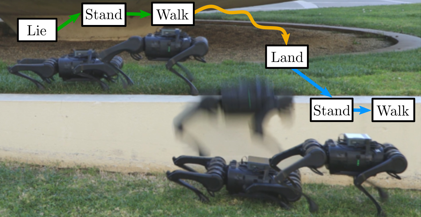
There are extensive studies of robust autonomy on dynamic systems [9, 10, 11, 12]. However, success typically relies on transition-specific analysis or heuristic conditions to determine switching behavior between dynamic primitive behaviors (commonly referred to as motion primitives [13, 14, 15, 16]). There is significant active work developing individual motion primitives for various dynamic systems [17, 18, 19], and capability is rapidly increasing in both volume and complexity. If we are to effectively incorporate increasingly complex behaviors into a dynamic autonomous system, we require a more formal method to determine appropriate transitions, both in nominal operation and in response to disturbances.

With this motivation, we build upon previous work on motion primitive transitions [16] where only discrete motion primitives and offline search were considered, and is limited in usefulness in regards to robustness. This manuscript extends the definition of motion primitives to include continuous arguments, develops a method for online search, and provides a methodology to manage the resulting complexity. We rely on notions of stability and regions of attraction to determine transition conditions [20, 21] and construct an abstraction of the dynamics that captures the mapping of dynamic state across the application of a motion primitive. This leads to a natural mixed discrete and continuous motion primitive graph that scales in complexity with number of primitives and associated arguments rather than the system dynamics. Inspired by the success of probabilistic search on similar problems, [22, 23], we propose a motion primitive graph search algorithm capable of continuous planning towards a desired motion primitive in both nominal and disturbed conditions. This summary represents the main contribution of this paper – a method to plan through motion primitive transitions despite underlying dynamics and complexity.

This procedure is applied to a quadrupedal robot with a set of motion primitives. Several experiments across a variety of environmental and antagonistic disturbances are successfully performed, and the results and accompanying video highlight the contributions of this work.

II Preliminaries

For the duration of this manuscript, we consider a nonlinear system in control affine form. We have system dynamics

$$\dot{x}=f(x)+g(x)u$$ (1)

with state $x\in\mathcal{X}\subset\mathbb{R}^{n}$ and control inputs $u\in\mathcal{U}\subset\mathbb{R}^{n}$. The functions ${f:\mathcal{X}\to\mathbb{R}^{n}}$ and ${g:\mathcal{X}\to\mathbb{R}^{n\times m}}$ are assumed to be locally Lipschitz continuous. The flow of this system, $\phi_{t}(x_{0})$, is solution to the initial value problem with $x(0)=x_{0}$. The Lipschitz assumptions give that $\phi_{t}(x_{0})$ is unique and, assuming forward completeness, exists for all $t\geq 0$.

II-A Motion Primitives

While the idea of motion primitives is not new, we introduce our own definition specifically suited for our purposes. This definition is generalization of the definition from previous work [16] to a larger class of motion primitives.

Definition 1.

A motion primitive is a dynamic behavior of (1) defined by the 6-tuple $\mathcal{P}={(\Xi,x^{*},k,\Omega,\mathcal{C},\mathcal{S})}$ with the following attributes:

• The valid arguments, $\Xi\subset\mathbb{R}^{a}$. This is the bounded set of continuous arguments that specifies the motion primitive’s behavior.

• The setpoint, ${x^{*}(x_{0},\xi,t):\mathcal{X}\times\Xi\times\mathbb{R}\to\mathcal{X}}$, that describes the desired state as a function of initial state, arguments, and time. It satisfies (1) and hence ${x^{*}(x_{0},\xi,t+t_{0})=\phi_{t}(x^{*}(x_{0},\xi,t_{0}),\xi)}$, ${\forall t\geq 0,t_{0}\in\mathbb{R}}$. It may be executed with a selected initial time $t_{0}$. $x^{*}$ must be differentiable with respect to $\xi$ and $t$ over the safe region of attraction ($\mathcal{S}(x^{*}(\cdot),\xi)$, as defined below).

• The control law, ${k:\mathcal{X}\times\Xi\times\mathbb{R}\to\mathcal{U}}$, that determines the control input ${u=k(x,\xi,t)}$. It is assumed to render the setpoint locally exponentially stable on the region of attraction ($\Omega(x^{*}(\cdot),\xi)$, as below). For constants $M,\alpha>0\in\mathbb{R},$ all $t>t_{0}$ and $x_{0}\in\Omega(x^{*}(\cdot),\xi_{0})$ implies:

  $$||\phi_{t-t_{0}}(x_{0})-x^{*}(\cdot)||\leq Me^{-\alpha(t-t_{0})}||x_{0}-x^{*}(\cdot)||$$ (2)

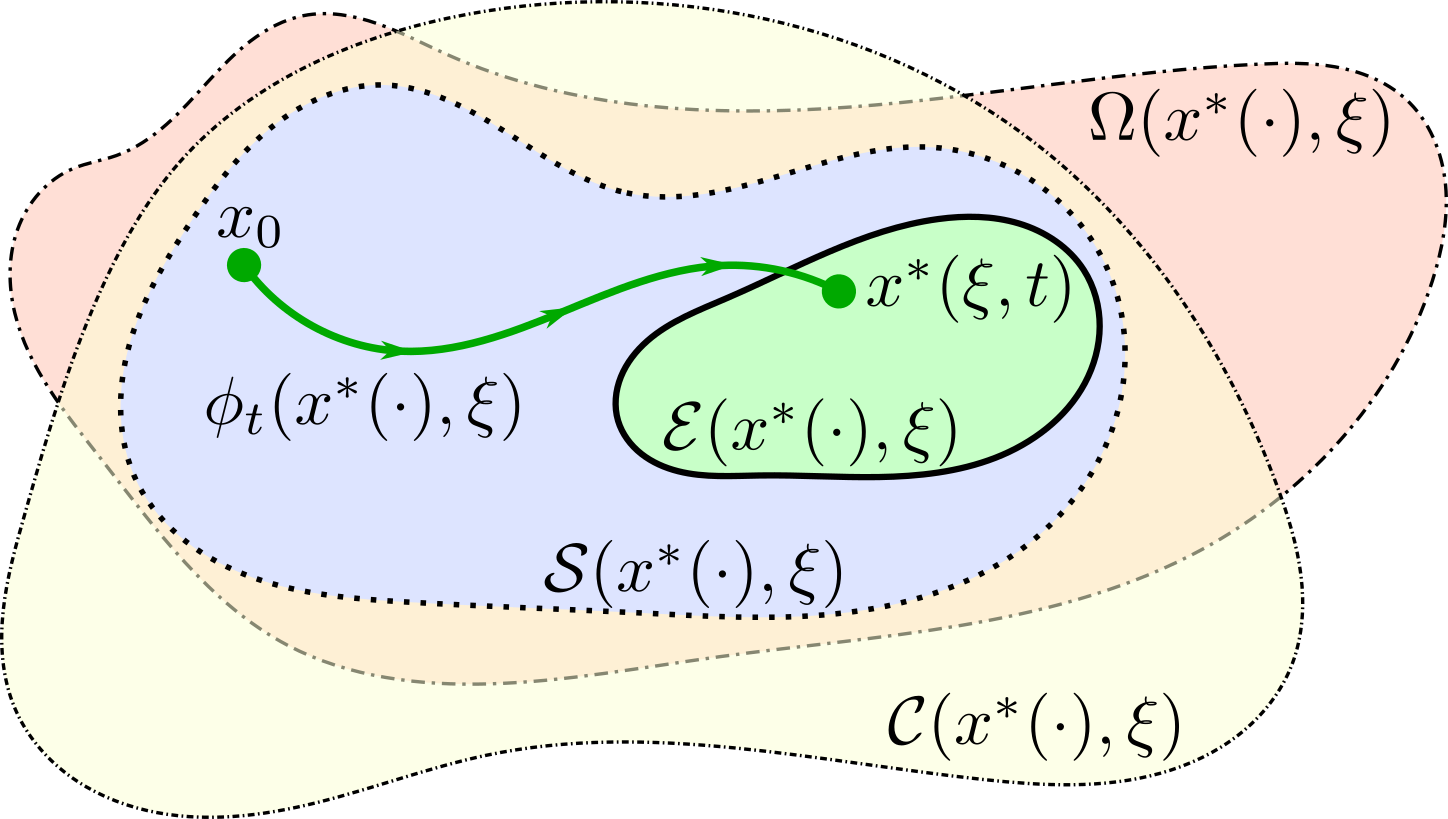
• The region of attraction (RoA) of the setpoint, ${\Omega:\mathcal{X}\times\Xi\to\mathscr{P}(\mathcal{X})}$, given by ${\Omega(x^{*}(\cdot),\xi)\subseteq\mathcal{X}}$:

  $$\Omega(x^{*}(\cdot),\xi)=\{ x_{0}\in\mathcal{X}:$$

  $$\lim_{t\to\infty}\phi_{t}(x_{0})\!-\!x^{*}(x_{0},\xi,t\!+\!t_{0})=0\}.$$

• The safe set, ${\mathcal{C}:\mathcal{X}\times\Xi\to\mathscr{P}(\mathcal{X})}$, that indicates the states of safe operation by the set ${\mathcal{C}(x^{*}(\cdot),\xi)\subset\mathcal{X}}$. It is assumed that ${x^{*}(x_{0},\xi,t+t_{0})\in\mathcal{C}(t)}$, ${\forall t\geq 0,t_{0}\in\mathbb{R}}$. This is designer-specified, and it is important to note that ${x\in\mathcal{C}(x^{*}(\cdot),\xi)\centernot\Longleftrightarrow x\in\Omega(x^{*}(\cdot),\xi)}$.

• The safe region of attraction, ${\mathcal{S}:\mathcal{X}\times\Xi\to\mathscr{P}(\mathcal{X})}$, that defines the set of states from which the flow converges to the setpoint while being safe for all time:

  $$\mathcal{S}(x^{*}(\cdot),\xi)=\{ x_{0}\in\Omega(x^{*}(\cdot),\xi):$$

  $$\phi_{t}(x_{0},\xi,t)\in\mathcal{C}(x^{*}(\cdot),\xi),\forall t\geq 0\}.$$

A illustration of the relationship between motion primitive attributes can be seen in Figure 2 and elucidating examples can be found in Section IV-B.

Figure 2: Depiction of motion primitive attributes and their relationships. Note the dependence on $\xi$ and $x^{*}(x_{0},\xi,t)$.

II-B Motion Primitive Transfer Function

Proposition 1.

Consider a motion primitive with argument $\xi_{0}\in\Xi$, initial condition $x_{0}\in\mathcal{X}$ and setpoint $x^{*}(x_{0},\xi_{0},t)$. If $x_{0}\in\mathcal{S}(x^{*},\xi_{0})$. There exists a duration $\Delta t_{min}\geq 0,\Delta t_{min}\in\mathbb{R}$ for any small constant $\epsilon>0,\epsilon\in\mathbb{R}$ such that:

$$||\phi_{\Delta t_{min}}(x_{0})-x^{*}(x_{0},\xi_{0},t_{0}+\Delta t_{min})||<\epsilon$$ (3)

Proof.

Consider the control law for the primitive $k(x,\xi_{0},t)$. This control law is assumed to render $x^{*}(x_{0},\xi_{0},t)$ exponentially stable over $\Omega(x^{*}(\cdot),\xi_{0})$. Take constants $M,\alpha>0\in\mathbb{R}$ satisfying Inequality 2 and $\epsilon>0,\epsilon\in\mathbb{R}$. Consider:

$$Me^{-\alpha(t-t_{0})} ||x_{0}-x^{*}(\cdot)||<\epsilon$$

$$\Rightarrow t-t_{0} >\underbrace{-\frac{1}{\alpha}\log\left(\frac{\epsilon}{M||x_{0}-x^{*}(\cdot)||}\right)}_{\Delta t_{min}}$$

As $x_{0}\in\mathcal{S}(x^{*},\xi_{0})\subseteq\Omega(x^{*},\xi_{0})$, Inequality 2 $\Rightarrow$ Inequality 3 and we have the existence of $\Delta t_{min}$ as desired. ∎

Choosing $\epsilon$ so that the deviation is negligible (in practice, within the accuracy of sensing), allows us to build an abstraction of the motion primitive dynamics that we call the motion primitive transfer function.

Figure 3: Dynamics of and relationships between motion primitives are abstracted via the motion primitive transfer function, implicitly producing a mixed discrete and continuous graph.

Definition 2.

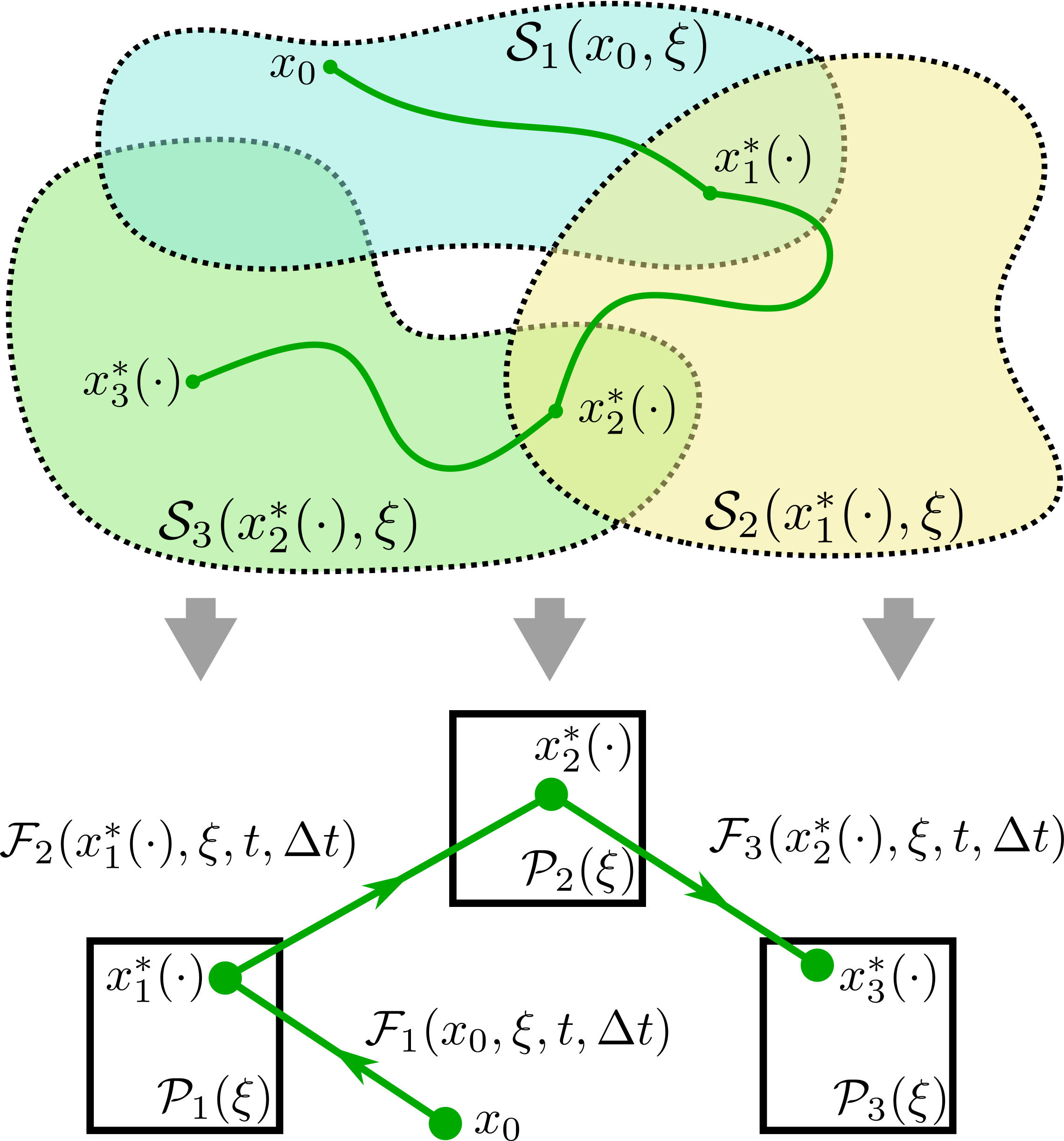
A motion primitive transfer function is a map $\mathcal{F}:\mathcal{X}\times\Xi\times\mathbb{R}\times\mathbb{R}\to\mathcal{X}$ that abstracts the dynamics of a motion primitive from input system state, arguments, initial time, and duration to an output system state:

$$\mathcal{F}(x_{0},\xi,t_{0},\Delta t)=\begin{cases}x^{*}(x_{0},\xi,t_{0}+\Delta t)&\text{if }x_{0}\in\mathcal{S}(x^{*}),\\ &\Delta t\geq\Delta t_{min}\\ x_{0}&\text{otherwise}\end{cases}$$ (4)

If the motion primitive is safe to use and our abstraction is valid, then this function returns the setpoint of the primitive. If it is unsafe or the duration is too short to ignore transient behavior, then the motion primitive cannot be applied, and the map simply returns the state unchanged.

Remark 1.

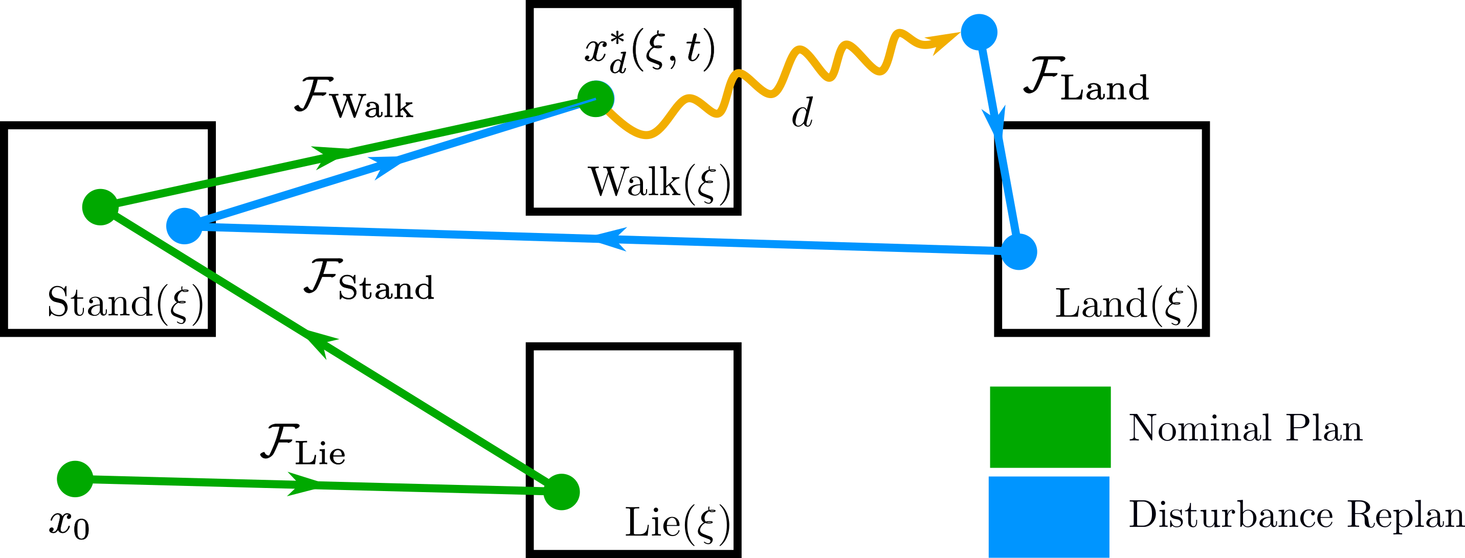
The motion primitive transfer function is composable in $x$, and a transition to a specific motion primitive from a arbitrary state can be found by chaining together motion primitive transfer functions, e.g. a sequence of transfer functions such that:

$$x^{*}_{1}(x_{0},\xi_{1},t_{1}) =\mathcal{F}_{1}(x_{0},\xi_{1},t_{1},\Delta t_{1})$$

$$x^{*}_{2}(x^{*}_{1},\xi_{2},t_{2}) =\mathcal{F}_{2}(x^{*}_{1},\xi_{2},t_{2},\Delta t_{2})$$

$$\;\;\vdots$$

$$x^{*}_{n}(x^{*}_{n-1},\xi_{n},t_{n}) =\mathcal{F}_{n}(x^{*}_{n-1},\xi_{n},t_{n},\Delta t_{n})$$

This construction builds a natural motion primitive graph structure in the state space of our system and the transition from an arbitrary state to a specific motion primitive is reduced to finding an appropriate path of motion primitive transfers. Namely, $\mathcal{R}=\{\mathcal{F}_{i}(\cdot,\xi_{i},t_{i},\Delta t_{i})$, $i=0,\ldots,n\}$ where $n$ corresponds to the desired motion primitive.

III Searching Mixed Discrete and Continuous Graph

In order to achieve robustness via motion primitive transitions, valid motion primitive transition paths used to react to disturbances and environmental uncertainties must be found in real time. Despite our abstraction of the motion primitive dynamics, searching quickly still poses a challenge. Typical methods, such as discrete search and pruning-based methods, scale unfavorably with the number motion primitives, size of the argument sets, and the dimensionality of the state space. Additionally, there is no expectation of convexity in the motion primitive transfer functions, posing difficulty for optimization-based methods.

There has been demonstrable success solving this class of search by using randomized search algorithms, including Rapidly-exploring Random Trees (RRT) [22], and variants. This class of algorithm can effectively search high-dimensional, nonconvex space, and is a natural choice for searching our motion primitive graph. We leverage this with an RRT-based search to discover feasible paths in the motion primitive graph, followed by constrained gradient descent and node-pruning post-processing.

III-A RRT-based Feasible Path Search Algorithm

Algorithm 1 FeasiblePathSearch

1:Node := {state, action, parent, cost to come, est. cost to go}

2:function FeasiblePathSearch ($\mathcal{P}_{d}(\xi_{d}),x_{0}$)

3:    $\mathcal{R}=\{\}$

4:    $n_{d}=\textsc{Node}(\emptyset)$

5:    $J_{\text{g}}=\textsc{Cost}(x^{*}_{d}(\cdot),x_{0}$)

6:    $n_{0}=\textsc{Node}(x_{0},\emptyset,\emptyset,0,J_{\text{g}})$

7:    $\mathcal{N}=\{n_{0}\}$

8:    $(n_{c},c)=(n_{0},J_{\text{g}})$

9:    while Node$(x^{*}_{d}(\cdot),\mathcal{F}_{d}(\cdot,\xi_{d},\cdot),\cdot)\not\in\mathcal{N}$ do

10:         $n_{s}=\textsc{Node}(\emptyset)$

11:         $u\thicksim U([0,1])$

12:         if $u<p$ then $\triangleright$ Sample the cheapest node

13:             $n_{s}=n_{c}$

14:         else$\triangleright$ Draw uniformly from existing nodes

15:             $n_{s}\thicksim U(\mathcal{N})$          

16:         $\mathcal{F}_{s}\thicksim U(\mathcal{F})$ $\triangleright$ Draw uniformly from transfer functions

17:         $\xi_{s}\thicksim U(\Xi_{s})$

18:         $t_{s}\thicksim U([t_{s_{min}},t_{s_{max}}])$

19:         $\Delta t_{s}\thicksim U([\Delta t_{s_{min}},\Delta t_{s_{min}}+t_{s_{max}}])$

20:         $x^{*}_{s}=\mathcal{F}_{s}(n_{s}.x,\xi_{s},t_{s},\Delta t_{s})$

21:         if $n_{s}.x\neq x^{*}_{s}$ then $\triangleright$ Add new node if $\mathcal{F}_{s}$ progresses

22:             $J_{\text{g}}=\textsc{Cost}(x^{*}_{d}(\cdot),x^{*}_{s}$)

23:             $J_{\text{c}}=\textsc{Cost}(x^{*}_{s},n_{s}.state)+n_{s}.{cost\_to\_come}$

24:             $\mathcal{N}.\text{push}(\textsc{Node}(x^{*}_{s},\mathcal{F}_{s},n_{s},J_{\text{c}},J_{\text{g}}))$

25:             if $J_{\text{g}}+J_{\text{c}}<c\ \textbf{then}$ $\triangleright$ Update cheapest node

26:                 $c=J_{\text{g}}+J_{\text{c}}$

27:                 $n_{c}=n_{s}$              

28:             if $x^{*}_{d}(\cdot)=\mathcal{F}_{d}(x^{*}_{s},\xi_{d},\cdot)$ then $\triangleright$ Check for goal

29:                 $J_{\text{c}}=\textsc{Cost}(x^{*}_{d},n_{s}.state)+n_{s}.{cost\_to\_come}$

30:                 $n_{d}=\textsc{Node}(x^{*}_{d},\mathcal{F}_{d},n_{s},J_{\text{c}},0))$

31:                 $\mathcal{R}=\{n_{d}\}$

32:                 break;                           

33:    $n=n_{d}$

34:    while $n.\text{parent}\neq\emptyset$ do $\triangleright$ Build final path

35:         $\mathcal{R}.\text{push\_front}(n)$

36:         $n=n.\text{parent}$     

37:    return $\mathcal{R}$

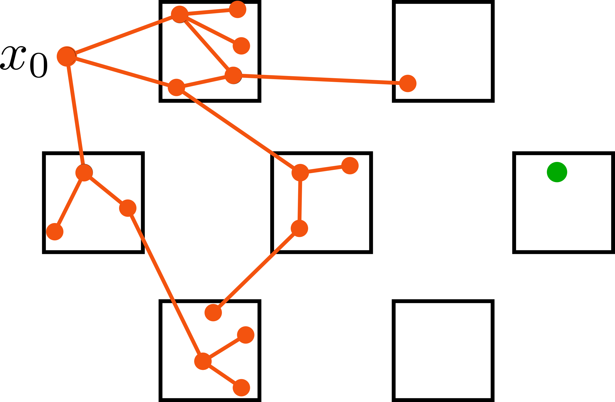
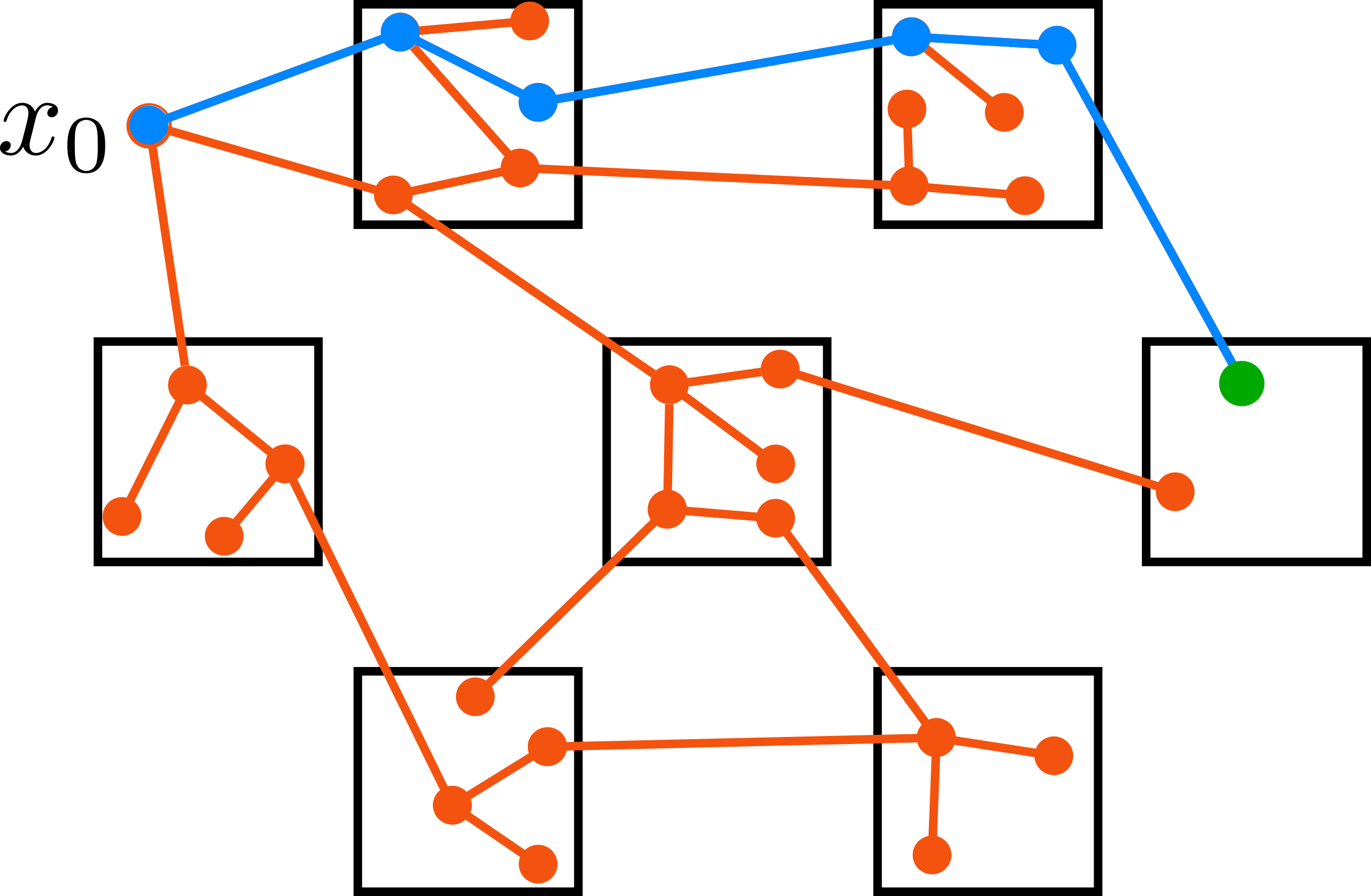
The first planning step, an RRT-inspired search, randomly expands a tree structure of nodes from an initial state ($x_{0}$), exploring the graph space until a feasible path to the desired primitive ($\mathcal{P}_{p}(\xi)$) is reached.

At each iteration, a node from the set of explored nodes is sampled. With probability $p$, this node is selected to be the cheapest node to encourage exploration towards the goal, otherwise the sampled node is taken uniformly. Next, a random motion primitive transfer function, corresponding arguments, and times are selected uniformly from their respective domains. If the sampled motion primitive transfer function makes progress, a new node is added as a child of the sampled node. As each new node is added, the cheapest node is updated, and one-step reachability of the goal is checked via $\mathcal{F}_{d}$, the transfer function associated with the desired motion primitive, $\mathcal{P}_{d}(\xi_{d})$.

Once the goal can be reached, the main iteration loop terminates, and the feasible path is returned. This is elucidated in Algorithm 1.

III-B Feasible Path Post-Processing

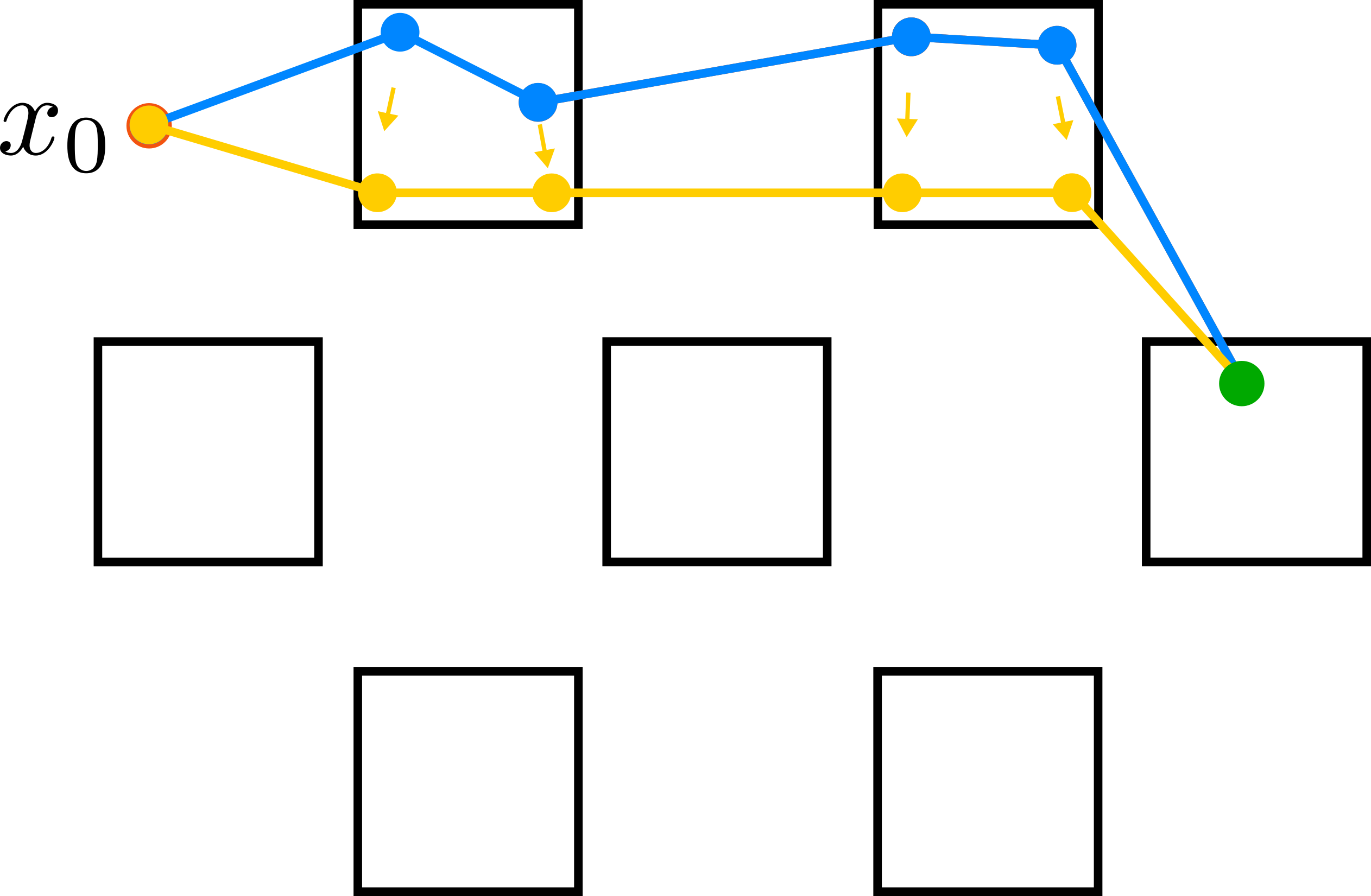
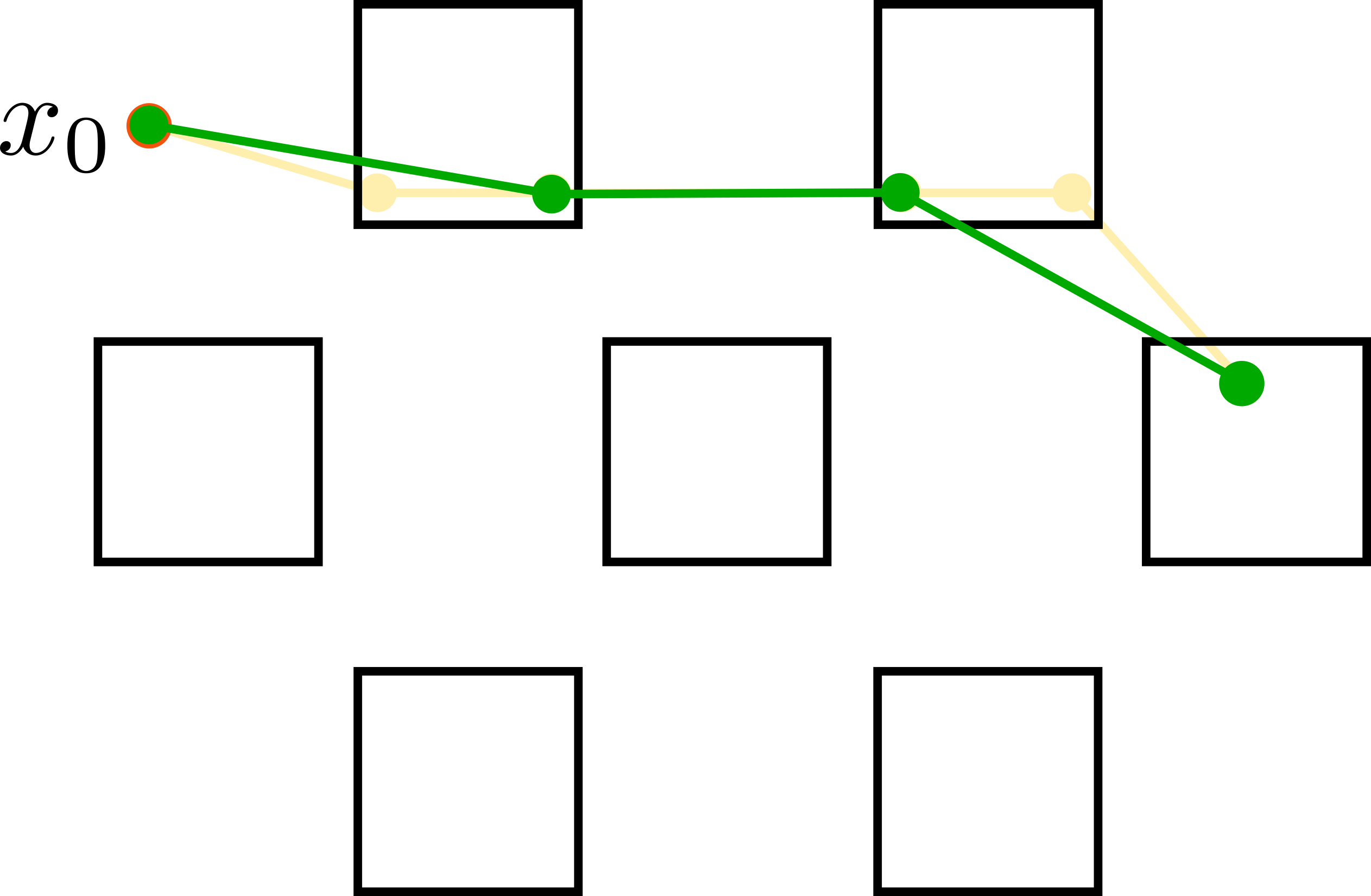
The feasible trajectory is then post-processed via two components: a constrained gradient descent and node-pruning. The constrained gradient descent intends to select the locally optimal $\xi,t_{0}$, and $\Delta t$ to minimize cost between nodes. Consider node $n_{i}$ with parent $n_{i-1}$ and child $n_{i+1}$. For differentiable cost function $J:\mathcal{X}\times\mathcal{X}\rightarrow\mathbb{R}$, we have local cost of $J_{i}\in\mathbb{R}$ as:

$$J_{i}=J(x^{*}_{i-1},x^{*}_{i})+J(x^{*}_{i},x^{*}_{i+1})$$ (5)

and cost gradient as:

$$\nabla J_{i} =\frac{\partial J_{i}}{\partial(\xi_{i},t_{i},\Delta t_{i})}=\frac{\partial J_{i}}{\partial x^{*}_{i}}\frac{\partial x^{*}_{i}}{\partial(\xi_{i},t_{i},\Delta t_{i})}$$

$$=\left(\frac{\partial J(x^{*}_{i-1},x^{*}_{i})}{\partial x^{*}_{i}}+\frac{\partial J(x^{*}_{i},x^{*}_{i+1})}{\partial x^{*}_{i}}\right)\frac{\partial x^{*}_{i}}{\partial(\xi_{i},t_{i},\Delta t_{i})}$$

As $J$ is differentiable and $x^{*}$ is differentiable in $\xi,t,\Delta t$, this gradient exists and is well-defined. Constraining $x^{*}_{i}\in\mathcal{S}_{i+i}$, we can apply constrained gradient descent [24] to find the locally optimal choice for $\xi_{i},t_{i}$, and $\Delta t_{i}$ for each node.

In node-pruning, unnecessary nodes in the feasible path are removed. That is, for candidate unnecessary node $i$ in path $\mathcal{R}$, if:

$$x^{*}_{1}(x_{0},\xi_{1},t_{1}) =\mathcal{F}_{1}(x_{0},\xi_{1},t_{1},\Delta t_{1})$$

$$\;\;\vdots$$

$$x^{*}_{i+1}(x^{*}_{i-1},\xi_{i+1},t_{i+1}) =\mathcal{F}_{i+1}(x^{*}_{i-1},\xi_{i+1},t_{i+1},\Delta t_{i+1})$$

$$\;\;\vdots$$

$$x^{*}_{n}(x^{*}_{n-1},\xi_{n},t_{n}) =\mathcal{F}_{n}(x^{*}_{n-1},\xi_{n},t_{n},\Delta t_{n})$$

is still a feasible path, then node $n_{i}$ can be bypassed and should be removed from $\mathcal{R}$. Each node in $\mathcal{R}$ is checked sequentially for this condition and removed as necessary.

Note that the constrained gradient descent and path pruning post-processing steps are coupled, and thus are intermingled iteratively to complete the post-processing of the feasible path. The entirety of this process is depicted in Figure 4. In practice, many paths can be computed in parallel, and the lowest cost among the paths taken as the result.

(a) Motion Primitive Graph with initial state $x_{0}$ and goal primitive $\mathcal{P}_{d}(\xi)$

(b) Feasible Path Search

(c) Feasible Path Found

(d) Constrained Gradient Descent in $\xi$

(e) Prune unnecessary nodes,
Final path found

Figure 4: Depiction of the search algorithm for the mixed discrete and continuous motion primitive transition graph. Boxes represent motion primitives and their continuous domain of arguments. Step (d) and (e) are iterated together.

IV Application to Quadrupeds

To investigate this work in a real-world application, the presented concepts are applied to the Unitree A1 quadrupedal robot with a experimental set of motion primitives. Here, we have configuration space $q\in\mathcal{Q}\subset\mathbb{R}^{n}$ with state space $x=(q,\dot{q})\in\mathcal{X}=T\mathcal{Q}\subset\mathbb{R}^{2n}$ with $n=18$. We have $m=12$ actuated degrees of freedom for control input $u\in\mathcal{U}\subset\mathbb{R}^{m}$. The hybrid-dynamic nature of the system leads to several domains of operation to be considered. These domains are marked by the contact state of each foot, denoted by a contact vector $c\in\{0,1\}^{|\mathcal{N}_{c}|}$ where $\mathcal{N}_{c}=\{1,2,3,4\}$ the set of considered contacts, in this case the quadruped’s feet. We consider and model no-slip via holonomic constraints $\psi(q)\equiv 0,\psi(q)\in\mathbb{R}^{h}$, where $h$ depends on the number of active contacts, i.e. the hybrid domain. We have our system dynamics for a specific domain in control affine form as:

$$\dot{x}=\underbrace{\begin{bmatrix}\dot{q}\\ -D(q)^{-1}(H(q,\dot{q})-J(q)^{\top}\lambda)\end{bmatrix}}_{f(x)}+\underbrace{\begin{bmatrix}0\\ D(q)^{-1}B\end{bmatrix}}_{g(x)}u,$$

where $D(q)\in\mathbb{R}^{n\times n}$ is the mass-inertia matrix, $H(q,\dot{q})\in\mathbb{R}^{n}$ accounts for the Coriolis and gravity terms, $B\in\mathbb{R}^{n\times m}$ is the actuation matrix, $J(q)=\frac{\partial c(q)}{\partial q}\in\mathbb{R}^{h}$ is the Jacobian of the holonomic constraints, and $\lambda\in\mathbb{R}^{h}$ is the constraint wrench. ${f:\mathcal{X}\to\mathcal{X}}$ and ${g:\mathcal{X}\to\mathbb{R}^{{2n}\times m}}$ are assumed to be locally Lipschitz continuous.

IV-A Quadruped Motion Primitives Preliminaries

Our experiments include several experimental motion primitives that utilize various control techniques to achieve their desired behavior. Though our method is agnostic to these implementation details and only requires that Definition 1 be satisfied, a brief discussion provides valuable context for realizing our method on a real system. We will begin by addressing some commonality between our test motion primitives.

Position and Velocity Safe Sets.

For all primitives, we can define the safe set for joint position and velocity limits as:

$$\mathcal{C}_{q,\dot{q}}=\{x\in\mathcal{X}:\; q_{\rm min}\leq q\leq q_{\rm max}, \dot{q}_{\rm min}\leq\dot{q}\leq\dot{q}_{\rm max}\}.$$

Computing Safe Regions of Attraction.

We consider an estimate $\mathcal{E}\subseteq\mathcal{S}$. There are several methods available to build $\mathcal{E}$, include Lyapunov-based methods [25, 26, 27], and backwards reachability analysis [28]. We employ a conservative construction from Lyapunov analysis of the linearization of the controller [29] and expand this region via hardware testing until the states of nominal operation are encompassed to produce conservative, but useful, formulations for $\mathcal{E}$.

IV-B Quadruped Motion Primitives in Experiments

Lie.

Lie is a motion primitive that rests the quadruped on the ground with the legs in a prescribed position. The feedback controller is a joint-space PD controller where $x^{*}(x_{0},t)$ is a cubic spline motion profile from the initial pose to the goal pose, $x^{*}_{\rm Lie}$. There are no continuous arguments, $\Xi=\emptyset$. In addition to the common safe set, the safe set for Lie requires at least one foot in contact with the ground, i.e.

$$\mathcal{C}_{\rm Lie}=\mathcal{C}_{q,\dot{q}}\cap\{x\in\mathcal{X}\;|\;\exists n_{c}\in\mathcal{N}_{c}\text{ where }c\{n_{c}\}=1\}$$

Stand.

The Stand motion primitive has setpoint $x^{*}_{\rm Stand}(\xi,t)$ to drive the body to specified height and orientation and center of mass to be above the centroid of the support polygon. Its trajectory is determined by a cubic spline in center of mass task-space. $\Xi=\{h,\theta_{x},\theta_{y},\theta_{z}\}$ with domain between bounds $\xi_{\rm min},\xi_{\rm max}$ derived from kinematic limits.

The control law is an Inverse-Dynamics Quadratic Program (ID-QP) including no-slip constraints on the feet. $\ddot{q}(x,t)$ in the objective function is specified by a task-space PD control law. Since this controller assumes ground contact of all feet, we require it via the safe set:

$$\mathcal{C}_{\rm Stand}=\mathcal{C}_{q,\dot{q}}\cap\{x\in\mathcal{X}\;|\;c\{n_{c}\}=1\quad\forall n_{c}\in\mathcal{N}_{c}\}$$

Walk.

The Walk primitive is a diagonal-gait walking trot, with arguments $\Xi=\{h,v_{x},v_{y},v_{\theta_{z}}\}$ and associated bounds corresponding to linear velocity in $x$ and $y$, angular velocity about the $z$ axis, and body height. As with Stand, walk uses an ID-QP based controller to track $x_{\rm walk}^{*}(\xi,t)$ in center of mass space, but in this case there is an additional component for a Raibert-style swing leg trajectory [30].

This controller assumes contact of the diagonal stance legs, so we have safe set as:

$$\mathcal{C}_{\rm Walk}(t)=\mathcal{C}_{q,\dot{q}}\cap\{x\in\mathcal{X}\;|\; c\{n_{c}\}=1\quad\forall n_{c}\in\mathcal{N}_{\rm stance}(t)\}$$

where $\mathcal{N}_{\rm stance}(t)\subset\mathcal{N}_{c}$ are the stance contacts at time $t$.

Land.

The Land primitive is a high-damping task-space PD control law on the position of the feet while the quadruped is airborne. The goal position of the feet is specified to maintain a constant support polygon, but the relative position of the center of the support polygon with respect to the center of mass is modulated according to a spring-loaded inverted pendulum model (SLIP) to remove all body velocity during the contact phase. The setpoint $x^{*}(x_{0},t)$ is derived from a ballistic trajectory given by the initial position and velocity and kinematics for the desired foot pose. The safe set for Land is simply the joint position and velocity safe set, $\mathcal{C}_{\rm Land}=\mathcal{C}_{q,\dot{q}}$.

IV-C Implementation and Experimental Results

Implementations for each experimental motion primitive and the algorithms described in Section III were built in our C++ motion primitive control framework. Here, the main control loop process runs 1kHz, and the motion primitive graph search runs in a separate thread asynchronously, with typical computation time less than 50 ms. The computation is done on a onboard Intel NUC with an i7-10710U CPU and 16GB of RAM.

(a) Kick During Stand: Differing magnitudes of disturbance elicit different responses.

(b) Leg Pull while Walking: Robustness to intentional disturbance while walking.

(c) Walking on Loose, Uneven Stones: Robustness to challenging walking environment

(d) Ledge Toss: Combination of disturbance and large environmental uncertainty

Figure 5: The experimental results of our proposed method exhibiting robustness across a variety of disturbances and conditions. Video of these results can be seen in the supplemental video [1].

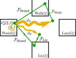
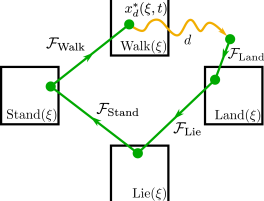
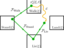
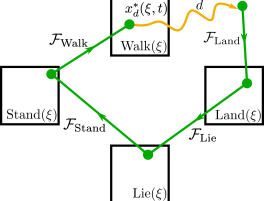
The specifics and results of each experiment are discussed below with details in Figure 5 and supplementary video [1]. Motion primitive commands are truncated for brevity when arguments are equal to zero, i.e. Stand($h=0.2$ m, $\theta_{x}=0$ rad, $\theta_{y}=0$ rad, $\theta_{z}=0$ rad) is shown as Stand($h=0.2$ m).

Nominal Transition to Walk.

Though emphasis in this work is achieving robustness via motion primitive transitions, it is implied that a nominal transition should be successful. In this experiment, the initial pose of the robot is at rest on the ground, with the motors unactuated. The commanded motion primitive is Walk$(h=0.25\textrm{ m},v_{x}=0.2\textrm{ m/s})$. From this position, the algorithm computes a sequence from the initial state to Lie(), Stand($h=0.2$ m), and then the goal, Walk$(h=0.25\textrm{ m},v_{x}=0.2\textrm{ m/s})$.

Kick During Stand.

The command motion primitive is Stand($h=0.25$ m), and subject to kick disturbances of varying magnitude. The Stand primitive has some inherent robustness, and when a small kick is applied, the state remains within the safe region of attraction and the system is stable to the setpoint without any transition. With a moderate kick, this is not the case, and the algorithm transitions through Lie before returning to standing at the desired height. With an even larger kick, a different plan is computed, transitioning to walking in place with Walk($h=0.25$) before returning to Stand($h=0.25$ m).

Leg Pull while Walking.

In this test, the desired primitive is Walk($h=0.25$ m, $v_{x}=0.2$ m/s). During the walk, the operator grabs a rear leg of the quadruped, providing some initial disturbance and preventing forward motion during the leg’s swing phase. In response, the sequence Land(), Stand($h=0.2$ m), Walk($h=0.25$ m, $v_{x}=0.2$ m/s) is computed. However, the continued disturbance prevents Lie() from being executed, and the system stays in the Land() primitive until the leg is released. At this point the recomputed plan can be finished and the quadruped resumes walking.

Walking on Loose, Uneven Stones.

The robot is commanded Walk($h=0.25$ m, $v_{x}=0.2$ m/s), but with a challenging environment consisting of loose, uneven stones. The stones cause the footfall height to vary across steps, and can be move when stepped on causing further deviation from the expected conditions. There is no perception involved and the walking primitive assumes flat terrain. In this test, the quadruped is able to progress slowly, taking steps and planning through the disturbances as they are encountered. Replans include transitioning through Lie() and Stand($\xi$) back to Walk, a single Stand($\xi$) to Walk, and in some cases, Land(), Lie(), Stand($\xi$), Walk($h=0.25$ m, $v_{x}=0.2$ m/s).

Ledge Toss.

In this experiment, the quadruped is tossed off an $\sim 0.5$ m high ledge while being commanded to Walk($h=0.25$ m, $v_{x}=0.2$ m/s). As the feet leave contact with the ground, the Land() primitive begins executing, and continues to execute until the state allows the transition to continue through Lie, Stand, and back to the desired Walk command.

V CONCLUSIONS

Motivated by the desire to achieve robust autonomy on dynamic robots, this paper has established a definition of motion primitives and used these attributes to construct an abstraction of the dynamics through the motion primitive transfer function. This formulation leads to a mixed discrete and continuous graph structure and we presented a probabilistic search algorithm with constrained gradient descent and node pruning post-processing to search this space for transition paths. The performance of this procedure allows for online replanning of paths through the motion primitive graph and can be used to reach the goal primitive in both nominal and disturbed scenarios. This was demonstrated on a quadrupedal robot for several experimental motion primitives subject to a variety of environmental and antagonistic disturbances.

While this represents a significant contribution to robust autonomy on dynamic systems, there are a number of extensions the authors would like to pursue. While a probabilistic approach is widely used in high-dimensional search problems and represents a natural starting point, there is additional structure to the problem ignored in this approach. As such, we intend to investigate how this structure may be incorporated into search to improve results. We would also like to extend this framework to the contexts with perception, and consider obstacles and varying environments explicitly. Future work intends address these avenues in the context of motion primitives and dynamic autonomy.

References

- [1] Supplemental Video, https://youtu.be/K3-xVWL08nk.
- [2] M. R. Pedersen et al., “Robot skills for manufacturing: From concept to industrial deployment,” Robotics and Computer-Integrated Manufacturing, vol. 37, pp. 282–291, 2016.
- [3] K. Edelberg et al., “Software system for the Mars 2020 mission sampling and caching testbeds,” in 2018 IEEE Aerospace Conference, 2018, pp. 1–11. [Online]. Available: https://app.dimensions.ai/details/publication/pub.1105216968
- [4] J. Bowkett et al., “Functional autonomy challenges in sampling for an Europa lander mission,” in 2021 IEEE Aerospace Conference (50100), 2021, pp. 1–8. [Online]. Available: https://app.dimensions.ai/details/publication/pub.1138696452
- [5] S. Karumanchi et al., “Team RoboSimian: Semi-autonomous mobile manipulation at the 2015 DARPA robotics challenge finals,” Journal of Field Robotics, vol. 34, pp. 305–332, 3 2017.
- [6] K. Edelberg et al., “Software system for the Mars 2020 mission sampling and caching testbeds,” in 2018 IEEE Aerospace Conference, 2018, pp. 1–11.
- [7] P. Backes et al., “The intelligent robotics system architecture applied to robotics testbeds and research platforms,” in 2018 IEEE Aerospace Conference, 2018, pp. 1–8.
- [8] P. Kim, B. C. Williams, and M. Abramson, “Executing reactive, model-based programs through graph-based temporal planning,” in International Joint Conference on Artificial Intelligence. Citeseer, 2001, pp. 487–493.
- [9] Boston Dynamics, “Atlas, The Next Generation,” accessed 2022-02-01. [Online]. Available: https://www.youtube.com/watch?v=rVlhMGQgDkY
- [10] H.-W. Park, A. Ramezani, and J. W. Grizzle, “A finite-state machine for accommodating unexpected large ground-height variations in bipedal robot walking,” IEEE Transactions on Robotics, vol. 29, no. 2, pp. 331–345, 2013.
- [11] D. O. Sales, D. O. Correa, L. C. Fernandes, D. F. Wolf, and F. S. Osório, “Adaptive finite state machine based visual autonomous navigation system,” Engineering Applications of Artificial Intelligence, vol. 29, pp. 152–162, 2014.
- [12] A. Singletary, T. Gurriet, P. Nilsson, and A. D. Ames, “Safety-critical rapid aerial exploration of unknown environments,” in 2020 IEEE International Conference on Robotics and Automation (ICRA). IEEE, 2020, pp. 10 270–10 276.
- [13] H. Zhao, M. J. Powell, and A. D. Ames, “Human-inspired motion primitives and transitions for bipedal robotic locomotion in diverse terrain,” Optimal Control Applications and Methods, vol. 35, pp. 730–755, 11 2014.
- [14] A. A. Paranjape, K. C. Meier, X. Shi, S.-J. Chung, and S. Hutchinson, “Motion primitives and 3D path planning for fast flight through a forest,” The International Journal of Robotics Research, vol. 34, no. 3, pp. 357–377, 2015.
- [15] A. Singla, S. Bhattacharya, D. Dholakiya, S. Bhatnagar, A. Ghosal, B. Amrutur, and S. Kolathaya, “Realizing learned quadruped locomotion behaviors through kinematic motion primitives,” in 2019 International Conference on Robotics and Automation (ICRA), 2019, pp. 7434–7440.
- [16] W. Ubellacker, N. Csomay-Shanklin, T. G. Molnar, and A. D. Ames, “Verifying safe transitions between dynamic motion primitives on legged robots,” in 2021 IEEE/RSJ International Conference on Intelligent Robots and Systems (IROS), 2021, pp. 8477–8484.
- [17] D. Kim, J. Di Carlo, B. Katz, G. Bledt, and S. Kim, “Highly dynamic quadruped locomotion via whole-body impulse control and model predictive control,” arXiv preprint arXiv:1909.06586, 2019.
- [18] F. Gómez-Bravo, F. Cuesta, and A. Ollero, “Parallel and diagonal parking in nonholonomic autonomous vehicles,” Engineering Applications of Artificial Intelligence, vol. 14, no. 4, pp. 419–434, 2001.
- [19] D. Falanga, A. Zanchettin, A. Simovic, J. Delmerico, and D. Scaramuzza, “Vision-based autonomous quadrotor landing on a moving platform,” in 2017 IEEE International Symposium on Safety, Security and Rescue Robotics (SSRR). IEEE, 2017, pp. 200–207.
- [20] R. Tedrake, “LQR-Trees: Feedback motion planning on sparse randomized trees,” 2009.
- [21] Á. Sousa, L. Silva, W. Lucia, and V. Leite, “Command governor strategy based on region of attraction control switching,” in Congresso Brasileiro de Automática-2020. SBA, 2020.
- [22] S. M. Lavalle, “Rapidly-exploring random trees: A new tool for path planning,” Tech. Rep., 1998.
- [23] L. Kavraki, P. Svestka, J.-C. Latombe, and M. Overmars, “Probabilistic roadmaps for path planning in high-dimensional configuration spaces,” IEEE Transactions on Robotics and Automation, vol. 12, no. 4, pp. 566–580, 1996.
- [24] S. Boyd, L. Xiao, and A. Mutapcic, “Subgradient methods,” lecture notes of EE392o, Stanford University, Autumn Quarter, vol. 2004, pp. 2004–2005, 2003.
- [25] E. Davison and E. Kurak, “A computational method for determining quadratic Lyapunov functions for non-linear systems,” Automatica, vol. 7, no. 5, pp. 627–636, 1971.
- [26] T. A. Johansen, “Computation of Lyapunov functions for smooth nonlinear systems using convex optimization,” Automatica, vol. 36, no. 11, pp. 1617–1626, 2000.
- [27] A. Polanski, “Lyapunov function construction by linear programming,” IEEE Transactions on Automatic Control, vol. 42, no. 7, pp. 1013–1016, 1997.
- [28] G. Yuan and Y. Li, “Estimation of the regions of attraction for autonomous nonlinear systems,” Transactions of the Institute of Measurement and Control, vol. 41, no. 1, pp. 97–106, 2019.
- [29] H. K. Khalil, “Nonlinear systems,” 2002.
- [30] M. H. Raibert, Legged robots that balance. MIT press, 1986.