DiP-GNN: Discriminative Pre-Training of
Graph Neural Networks

Abstract

Graph neural network (GNN) pre-training methods have been proposed to enhance the power of GNNs. Specifically, a GNN is first pre-trained on a large-scale unlabeled graph and then fine-tuned on a separate small labeled graph for downstream applications, such as node classification. One popular pre-training method is to mask out a proportion of the edges, and a GNN is trained to recover them. However, such a generative method suffers from graph mismatch. That is, the masked graph inputted to the GNN deviates from the original graph. To alleviate this issue, we propose DiP-GNN (Discriminative Pre-training of Graph Neural Networks). Specifically, we train a generator to recover identities of the masked edges, and simultaneously, we train a discriminator to distinguish the generated edges from the original graph’s edges. In our framework, the graph seen by the discriminator better matches the original graph because the generator can recover a proportion of the masked edges. Extensive experiments on large-scale homogeneous and heterogeneous graphs demonstrate the effectiveness of the proposed framework.

1 Introduction

Graph neural networks (GNNs) have achieved superior performance in various applications, such as node classification (Kipf & Welling, 2017), knowledge graph modeling (Schlichtkrull et al., 2018) and recommendation systems (Ying et al., 2018). To enhance the power of GNNs, generative pre-training methods are developed (Hu et al., 2020b). During the pre-training stage, a GNN incorporates topological information by training on a large-scale unlabeled graph in a self-supervised manner. Then, the pre-trained model is fine-tuned on a separate small labeled graph for downstream applications. Generative GNN pre-training is akin to masked language modeling in language model pre-training (Devlin et al., 2019). That is, for an input graph, we first randomly mask out a proportion of the edges, and then a GNN is trained to recover the original identity of the masked edges.

One major drawback with the abovementioned approach is graph mismatch. That is, the input graph to the GNN deviates from the original one since a considerable amount of edges are dropped. This causes changes in topological information, e.g., node connectivity. Consequently, the learned node embeddings may not be desirable.

To mitigate the above issues, we propose DiP-GNN, short for Discriminative Pre-training of Graph Neural Networks. In DiP-GNN, we simultaneously train a generator and a discriminator. The generator is trained in a similar way as existing generative pre-training approaches, where the model seeks to recover the masked edges and outputs a reconstructed graph. Subsequently, the reconstructed graph is fed to the discriminator, which predicts whether each edge resides in the original graph (i.e., a true edge) or is constructed by the generator (i.e., a fake edge). Figure 1 illustrates our training framework. Note that our work is related to Generative Adversarial Nets (GAN, Goodfellow et al. 2014), and detailed discussions are presented in Section 3.5. We remark that similar approaches have been used in natural language processing (Clark et al., 2020). However, we identify the graph mismatch problem (see Section 4.4), which is specific to graph-related applications and is not observed in natural language processing.

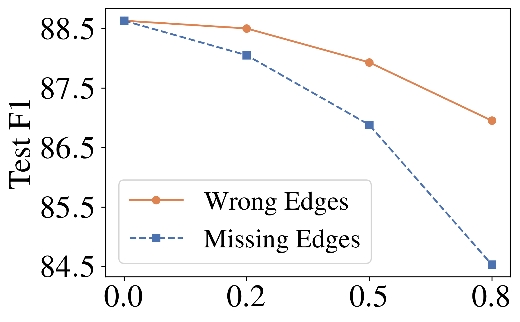
The proposed framework is more advantageous than generative pre-training. This is because the reconstructed graph fed to the discriminator better matches the original graph compared with the masked graph fed to the generator. Consequently, the discriminator can learn better node embeddings. Such a better alignment is because the generator recovers the masked edges during pre-training, i.e., we observe that nearly 40% of the missing edges can be recovered. We remark that in our framework, the graph fed to the generator has missing edges, while the graph fed to the discriminator contains wrong edges since the generator may make erroneous predictions. However, empirically we find that missing edges hurt more than wrong ones, making discriminative pre-training more desirable (see Section 4.4 in the experiments).

Figure 1: Illustration of DiP-GNN. From left to right: Original graph; Graph with two masked edges (dashed lines); Reconstructed graph created by the generator (generated edges are the dashed red lines); Discriminator labels each edge as [G] (generated) or [O] (original), where there are two wrong labels (shown in red).

We demonstrate effectiveness of DiP-GNN on large-scale homogeneous and heterogeneous graphs. Results show that the proposed method significantly outperforms existing generative pre-training and self-supervised learning approaches. For example, on the homogeneous Reddit dataset (Hamilton et al., 2017) that contains 230k nodes, we obtain an improvement of 1.1 in terms of F1 score; and on the heterogeneous OAG-CS graph (Tang et al., 2008) that contains 1.1M nodes, we obtain an improvement of 2.8 in terms of MRR score in the paper field prediction task.

2 Background

$\diamond$ Graph Neural Networks. Graph neural networks compute a node’s representation by aggregating information from the node’s neighbors. Concretely, for a multi-layer GNN, the feature vector $h_{v}^{(k)}$ of node $v$ at the $k$-th layer is

$$a_{v}^{(k)}=\mathrm{Aggregate}\left(\left\{h_{u}^{(k-1)}\ \forall u\in\mathrm{Neighbor}(v)\right\}\right),\ h_{v}^{(k)}=\mathrm{Combine}\left(a_{v}^{(k)},h_{v}^{(k-1)}\right),$$

where $\mathrm{Neighbor}(v)$ denotes all the neighbor nodes of $v$. Various implementations of $\mathrm{Aggregate}(\cdot)$ and $\mathrm{Combine}(\cdot)$ are proposed for both homogeneous (Defferrard et al., 2016; Kipf & Welling, 2017; Velickovic et al., 2018; Xu et al., 2019) and heterogeneous graphs (Schlichtkrull et al., 2018; Wang et al., 2019; Zhang et al., 2019; Hu et al., 2020c).

$\diamond$ Graph Neural Network Pre-Training. Previous unsupervised learning methods leverage the graph’s proximity (Tang et al., 2015) or information gathered by random walks (Perozzi et al., 2014; Grover & Leskovec, 2016; Dong et al., 2017; Qiu et al., 2018). However, the learned embeddings cannot be transferred to unseen nodes, limiting the methods’ applicability. Other unsupervised learning algorithms adopt contrastive learning (Hassani & Ahmadi, 2020; Qiu et al., 2020; Zhu et al., 2020; 2021; You et al., 2020; 2021). That is, we generate two views of the same graph, and then maximize agreement of node presentations in the two views. However, our experiments reveal that these methods do not scale well to extremely large graphs with millions of nodes.

Many GNN pre-training methods focus on generative objectives. For example, GAE (Graph Auto-Encoder, Kipf & Welling 2016) proposes to reconstruct the graph structure; GraphSAGE (Hamilton et al., 2017) optimizes an unsupervised loss derived from a random-walk-based metric; and DGI (Deep Graph Infomax, Velickovic et al. 2019) maximizes the mutual information between node representations and a graph summary representation.

There are also pre-training methods that extract graph-level representations, i.e., models are trained on a large amount of small graphs instead of a single large graph. For example, Hu et al. 2020a propose pre-training methods that operate on both graph and node level; and InfoGraph (Sun et al., 2020) proposes to maximize the mutual information between graph representations and representations of the graphs’ sub-structures. In this work, we focus on pre-training GNNs on a single large graph instead of multiple small graphs.

3 Method

We formally introduce the proposed discriminative GNN pre-training framework DiP-GNN. The algorithm contains two ingredients: edge generation/discrimination and feature generation/discrimination.

3.1 Edge Generation and Discrimination

Suppose we have a graph $\mathcal{G}=(\mathcal{N},\mathcal{E})$, where $\mathcal{N}$ denotes all the nodes and $\mathcal{E}$ denotes all the edges. We randomly mask out a proportion of the edges, such that $\mathcal{E}=\mathcal{E}_{u}\cup\mathcal{E}_{m}$, where $\mathcal{E}_{u}$ is the unmasked set of edges and $\mathcal{E}_{m}$ is the set of edges that are masked out.

For a masked edge $e=(n_{1},n_{2})\in\mathcal{E}_{m}$, where $n_{1}$ and $n_{2}$ are the two nodes connected by $e$, the generator’s goal is to predict $n_{1}$ given $n_{2}$ and the unmasked edges $\mathcal{E}_{u}$. For each node $n$, we compute its representation $h_{g}(n)=f^{e}_{g}(n,\theta_{g}^{e})$ using the generator $f^{e}_{g}(\cdot,\theta_{g}^{e})$, which is parameterized by $\theta_{g}^{e}$. We remark that the computation of $h_{g}(\cdot)$ only relies on the unmasked edges $\mathcal{E}_{u}$. We assume that the generation process of each edge is independent. Then, we have the following generation process

$$p(n_{1}|n_{2},\mathcal{E}_{u})=\frac{\exp\left(d(h_{g}(n_{1}),h_{g}(n_{2}))\right)}{\sum_{n^{\prime}\in\mathcal{C}}\exp\left(d(h_{g}(n^{\prime}),h_{g}(n_{2}))\right)},\quad\widehat{n}_{1}=\underset{n^{\prime}\in\mathcal{C}}{\mathrm{argmax}}\ p(n^{\prime}|n_{2},\mathcal{E}_{u}).$$ (1)

In the above equations, $\mathcal{C}$ is the candidate set for $n_{1}$ obtained by negative sampling (see Section 3.4 for details). Moreover, the distance function $d(\cdot,\cdot)$ is chosen as a trainable cosine similarity, i.e.,

$$d(u,v)=\frac{(W^{\mathrm{cos}}u)^{\top}v}{||W^{\mathrm{cos}}u||\cdot||v||},$$ (2)

where $W^{\mathrm{cos}}$ is a trainable weight. We repeat this generation process for every masked edge in $\mathcal{E}_{m}$, after which we obtain a set of generated edges $\mathcal{E}_{g}=\{(\widehat{n}_{1},n_{2})\}_{(n_{1},n_{2})\in\mathcal{E}_{m}}$. The training loss for the generator is defined as

$$\mathcal{L}^{e}_{g}(\theta_{g}^{e})=\sum_{(n_{1},n_{2})\in\mathcal{E}_{m}}-\log p(n_{1}|n_{2},\mathcal{E}_{u}).$$

The discriminator is trained to distinguish edges that are from the original graph and edges that are generated. Specifically, given the unmasked edges $\mathcal{E}_{u}$ and the generated ones $\mathcal{E}_{g}$, we first compute $h_{d}(n)=f^{e}_{d}(n,\theta_{d}^{e})$ for every node $n\in\mathcal{N}$, where $f^{e}_{d}(\cdot,\theta_{d}^{e})$ is the discriminator model parameterized by $\theta_{d}^{e}$. We highlight that different from computing $h_{g}(\cdot)$, the computation of $h_{d}(\cdot)$ relies on both $\mathcal{E}_{u}$ and $\mathcal{E}_{g}$, such that the discriminator can separate a generated edge from an original one. Then, for each edge $e=(n_{1},n_{2})\in\mathcal{E}_{u}\cup\mathcal{E}_{g}$, the discriminator outputs

$$p(e\in\mathcal{E}_{g}|\mathcal{E}_{u},\mathcal{E}_{g})=\mathrm{sigmoid}\left(d(h_{d}(n_{1}),h_{d}(n_{2}))\right),$$

where $d(\cdot,\cdot)$ is the distance function in Eq. 2. The training loss for the discriminator is

$$\mathcal{L}^{e}_{d}(\theta_{d}^{e})=\sum_{e\in\mathcal{E}_{u}\cup\mathcal{E}_{g}}-\mathbf{1}\{e\in\mathcal{E}_{g}\}\log p(e\in\mathcal{E}_{g}|\mathcal{E}_{u},\mathcal{E}_{g})-\mathbf{1}\{e\in\mathcal{E}_{u}\}\log(1-p(e\in\mathcal{E}_{g}|\mathcal{E}_{u},\mathcal{E}_{g})),$$

where $\mathbf{1}\{\cdot\}$ is the indicator function.

The edge loss is the weighted sum of the generator’s and the discriminator’s loss

$$\mathcal{L}^{e}(\theta_{g}^{e},\theta_{d}^{e})=\mathcal{L}_{g}^{e}(\theta_{g}^{e})+\lambda\mathcal{L}_{d}^{e}(\theta_{d}^{e}),$$

where $\lambda$ is a hyper-parameter. Note that structures of the generator $f_{g}$ and the discriminator $f_{d}$ are flexible, e.g., they can be graph convolutional networks (GCN) or graph attention networks (GAT).

3.2 Feature Generation and Discrimination

In real-world applications, a node in a graph is often associated with features. For example, in the Reddit dataset (Hamilton et al., 2017), a node’s feature is a vectorized representation of the post corresponding to the node. As another example, in citation networks (Tang et al., 2008), a paper’s title can be treated as a node’s feature. Previous work (Hu et al., 2020b) has demonstrated that generating features and edges simultaneously can improve the GNN’s representation power.

Node features can be either texts (e.g., in citation networks) or vectors (e.g., in recommendation systems). In this section, we develop feature generation and discrimination procedures for texts. Vector features are akin to encoded text features, and we can use linear layers to generate and discriminate them. Details about vector features are deferred to Appendix B.

For text features, we parameterize both the feature generator and the feature discriminator using bi-directional Transformer models (Vaswani et al., 2017), similar to BERT (Devlin et al., 2019). Denote $f^{f}_{g}(\cdot,\theta_{g}^{f})=\mathrm{trm}_{g}\circ\mathrm{emb}_{g}(\cdot)$ the generator parameterized by $\theta_{g}^{f}$, where $\mathrm{emb}_{g}$ is the word embedding function and $\mathrm{trm}_{g}$ denotes subsequent Transformer layers. For an input text feature $\mathbf{x}=[x_{1},\cdots,x_{L}]$ where $L$ is the sequence length, we randomly select indices to mask out, i.e., we randomly select an index set $\mathcal{M}\subset\{1,\cdots,L\}$. For a masked position $i\in\mathcal{M}$, the generation probability is given by

$$p(x_{i}|\mathbf{x})=\frac{\exp\left(\mathrm{emb}_{g}(x_{i})^{\top}v_{g}(x_{i})\right)}{\sum_{x^{\prime}\in\mathrm{vocab}}\exp\left(\mathrm{emb}_{g}(x^{\prime})^{\top}v_{g}(x^{\prime})\right)},\quad v_{g}(x_{i})=\mathrm{trm}_{g}\left(W_{g}^{\mathrm{proj}}\left[h_{g}(n_{\mathbf{x}}),\mathrm{emb}_{g}(x_{i})\right]\right).$$

Here $W_{g}^{\mathrm{proj}}$ is a trainable weight and $h_{g}(n_{\mathbf{x}})$ is the representation of the node corresponding to $\mathbf{x}$ computed by the edge generation GNN. Note that we concatenate the text embedding $\mathrm{emb}_{g}(x_{i})$ and the feature node’s embedding $h_{g}(n_{\mathbf{x}})$, such that the feature generator can aggregate information from the graph structure. Then, the generator generates

$$\widehat{x}_{i}=\underset{x_{i}\in\mathrm{vocab}}{\mathrm{argmax}}\ p(x_{i}|\mathbf{x}).$$

This generation procedure is repeated for all the masked tokens, after which we obtain a new text feature $\mathbf{x}^{\text{corr}}$, where we set $x^{\text{corr}}_{i}=x_{i}$ for $i\notin\mathcal{M}$ and $x_{i}^{\text{corr}}=\widehat{x}_{i}$ for $i\in\mathcal{M}$. The training loss for the generator is

$$\mathcal{L}^{f}_{g}(\theta_{g}^{e},\theta_{g}^{f})=\sum_{\mathbf{x}}\sum_{i\in\mathcal{M}}-\log p(x_{i}|\mathbf{x}).$$

The discriminator is trained to distinguish the generated tokens from the original ones in $\mathbf{x}^{\text{corr}}$. Similar to the generator, we denote $f_{d}^{f}(\cdot,\theta_{d}^{f})=\mathrm{trm}_{d}\circ\mathrm{emb}_{d}(\cdot)$ as the discriminator parameterized by $\theta_{d}^{f}$. For each position $i$, the discriminator’s prediction probability is defined as

$$p(x^{\text{corr}}_{i}=x_{i})=\mathrm{sigmoid}\left(w^{\top}v_{d}(x^{\text{corr}}_{i})\right),\text{ where }v_{d}(x^{\text{corr}}_{i})=\mathrm{trm}_{d}\left(W_{d}^{\mathrm{proj}}\left[h_{d}(n_{\mathbf{x}}),\mathrm{emb}_{d}(x^{\text{corr}}_{i})\right]\right).$$

Here $w$ and $W_{d}^{\mathrm{proj}}$ are trainable weights and $h_{d}(n_{\mathbf{x}})$ is the representation of the node corresponding to $\mathbf{x}$ computed by the edge discriminator GNN. The training loss for the discriminator is

$$\mathcal{L}_{d}^{f}(\theta_{d}^{e},\theta_{d}^{f})=\sum_{\mathbf{x}}\sum_{i=1}^{L}-\mathbf{1}\{x^{\text{corr}}_{i}=x_{i}\}\log p(x^{\text{corr}}_{i}=x_{i})-\mathbf{1}\{x^{\text{corr}}_{i}\neq x_{i}\}\log(1-p(x^{\text{corr}}_{i}=x_{i})).$$

The text feature loss is defined as

$$\mathcal{L}^{f}(\theta_{g}^{e},\theta_{g}^{f},\theta_{d}^{e},\theta_{d}^{f})=\mathcal{L}_{g}^{f}(\theta_{g}^{e},\theta_{g}^{f})+\lambda\mathcal{L}_{d}^{f}(\theta_{d}^{e},\theta_{d}^{f}),$$

where $\lambda$ is a hyper-parameter.

3.3 Model Training

We jointly minimize the edge loss and the feature loss, where the loss function is

$$\mathcal{L}(\theta_{g}^{e},\theta_{g}^{f},\theta_{d}^{e},\theta_{d}^{f}) =\mathcal{L}^{e}(\theta_{g}^{e},\theta_{d}^{e})+\mathcal{L}^{f}(\theta_{g}^{e},\theta_{g}^{f},\theta_{d}^{e},\theta_{d}^{f})$$

$$=\left(\mathcal{L}_{g}^{e}(\theta_{g}^{e})+\mathcal{L}_{g}^{f}(\theta_{g}^{e},\theta_{g}^{f})\right)+\lambda\left(\mathcal{L}_{d}^{e}(\theta_{d}^{e})+\mathcal{L}_{d}^{f}(\theta_{d}^{e},\theta_{d}^{f})\right).$$ (3)

Here, $\lambda$ is the weight of the discriminator’s loss. We remark that our framework is flexible because the generator’s loss ($\mathcal{L}_{g}^{e}$ and $\mathcal{L}_{g}^{f}$) is decoupled from the discriminator’s ($\mathcal{L}_{d}^{e}$ and $\mathcal{L}_{d}^{f}$). As such, existing generative pre-training methods can be applied to train the generator. After pre-training, we discard the generator and fine-tune the discriminator on downstream tasks. A detailed training pipeline is presented in Appendix A.

3.4 Implementation Details

$\diamond$ Graph subsampling. In practice, graphs are often too large to fit in the hardware, e.g., the Reddit dataset (Hamilton et al., 2017) contains over 230k nodes. Therefore, we sample a dense subgraph from the large-scale graph in each training iteration. For homogeneous graphs, we apply the LADIES algorithm (Zou et al., 2019), which theoretically guarantees that the sampled nodes are highly inter-connected with each other and can maximally preserve the graph structure. For heterogeneous graphs, we use the HGSampling algorithm (Hu et al., 2020b), which is a heterogeneous version of LADIES.

$\diamond$ Node sampling for the edge generator. In the edge generator, for a masked edge $(s,t)$, we fix the node $t$ and seek to identify the other node $s$. One approach is to identify $s$ from all the graph nodes, i.e., by setting $\mathcal{C}=\mathcal{N}$ in Eq. 1. However, this task is computationally intractable when the number of nodes is large, i.e., the model needs to find $s$ out of hundreds of thousands of nodes. Therefore, we sample some negative nodes $\{s^{g}_{i}\}_{i=1}^{n_{\text{neg}}}$ such that $(s_{i}^{g},t)\notin\mathcal{E}$. Then, the candidate set to generate the source node becomes $\{s,s_{1}^{g},\cdots,s_{n_{\text{neg}}}^{g}\}$ instead of all the graph nodes $\mathcal{N}$. We remark that such a sampling approach is standard for GNN pre-training and link prediction (Hamilton et al., 2017; Sun et al., 2020; Hu et al., 2020b).

$\diamond$ Edge sampling for the edge discriminator. In computing the loss for the discriminator, the number of edges in $\mathcal{E}_{u}$ is significantly larger than those in $\mathcal{E}_{g}$, i.e., we only mask a small proportion of the edges. To avoid the discriminator from outputting trivial predictions (i.e., all the edges belong to $\mathcal{E}_{u}$), we balance the two loss terms in $\mathcal{L}_{d}^{e}$. Specifically, we sample $\mathcal{E}_{u}^{d}\subset\mathcal{E}_{u}$ such that $|\mathcal{E}_{u}^{d}|=\alpha|\mathcal{E}_{g}|$, where $\alpha$ is a hyper-parameter. Then, we compute $\mathcal{L}_{d}^{e}$ on $\mathcal{E}_{g}$ and $\mathcal{E}_{u}^{d}$. Note that the node representations $h_{d}$ are still computed using all the generated and unmasked edges $\mathcal{E}_{g}$ and $\mathcal{E}_{u}$.

3.5 Comparison with GAN

We remark that our framework is different from Generative Adversarial Nets (GAN, Goodfellow et al. 2014). In GAN, the generator-discriminator training framework is formulated as a min-max game, where the generator is trained adversarially to fool the discriminator. The two models are updated using alternating gradient descent/ascent.

However, the min-max game formulation of GAN is not applicable to our framework. This is because in GNN pre-trianing, the generator generates discrete edges, unlike continuous pixel values in the image domain. Such a property prohibits back-propagation from the discriminator to the generator. Existing works (Wang et al., 2018) use reinforcement learning (specifically policy gradient) to circumvent the non-differentiability issue. However, reinforcement learning introduces extensive hyper-parameter tuning and suffers from scalability issues. For example, the largest graph used in Wang et al. 2018 only contains 18k nodes, whereas the smallest graph used in our experiments has about 233k nodes.

Additionally, the goal of GAN is to train good-quality generators, which is different from our focus. In our discriminative pre-training framework, we focus on the discriminator because of better graph alignments. In practice, we find that accuracy of the generator is already high even without the discriminator, e.g., the accuracy is higher than 40% with 255 negative samples. And we observe that further improving the generator does not benefit downstream tasks.

4 Experiments

We implement all the algorithms using PyTorch (Paszke et al., 2019) and PyTorch Geometric (Fey & Lenssen, 2019). Experiments are conducted on NVIDIA A100 GPUs. By default, we use Heterogeneous Graph Transformer (HGT, Hu et al. 2020c) as the backbone GNN. We also discuss other choices in the experiments. Training and implementation details are deferred to Appendix C.

4.1 Settings and Datasets

$\diamond$ Settings. We consider a node transfer setting in the experiments. In practice we often work with a single large-scale graph, on which labels are sparse. In this case, we can use the large amount of unlabeled data as the pre-training dataset, and the rest are treated as labeled fine-tuning nodes. Correspondingly, edges between pre-training nodes are added to the pre-training data, and edges between fine-tuning nodes are added to the fine-tuning data. In this way, the model cannot see the fine-tuning data during pre-training, and vice versa.

We remark that our setting is different from conventional self-supervised learning settings, namely we pre-train and fine-tune on two separate graphs. This meets the practical need of transfer learning, e.g., a trained GNN needs to transfer across locales and time spans in recommendation systems.

$\diamond$ Homogeneous Graph. We use the Reddit dataset (Hamilton et al., 2017), which is a publicly available large-scale graph. In this graph, each node corresponds to a post, and is labeled with a “subreddit”. Each node has a 603-dimensional feature vector constructed from the corresponding post. Two nodes (posts) are connected if the same user commented on both. The dataset contains posts from 50 subreddits sampled from posts initiated in September 2014. In total, there are 232,965 posts with an average node degree of 492. We use 70% of the data as the pre-training data, and the rest as the fine-tuning data, which are further split into training, validation, and test sets equally. We consider node classification as the downstream fine-tuning task.

$\diamond$ Product Recommendation Graph. We collect in-house product recommendation data from an e-commerce website. We build a bi-partite graph with two node types: search queries and product ids. The dataset contains about 633k query nodes, 2.71M product nodes, and 228M edges. We sample 70% of the nodes (and corresponding edges) for pre-training, and the rest are evenly split for fine-tuning training, validation and testing. We consider link prediction as the downstream task, where for each validation and test query node, we randomly mask out 20% of its edges to recover. For each masked edge that corresponds to a query node and a positive product node, we randomly sample 255 negative products. The task is to find the positive product out of the total 256 products.

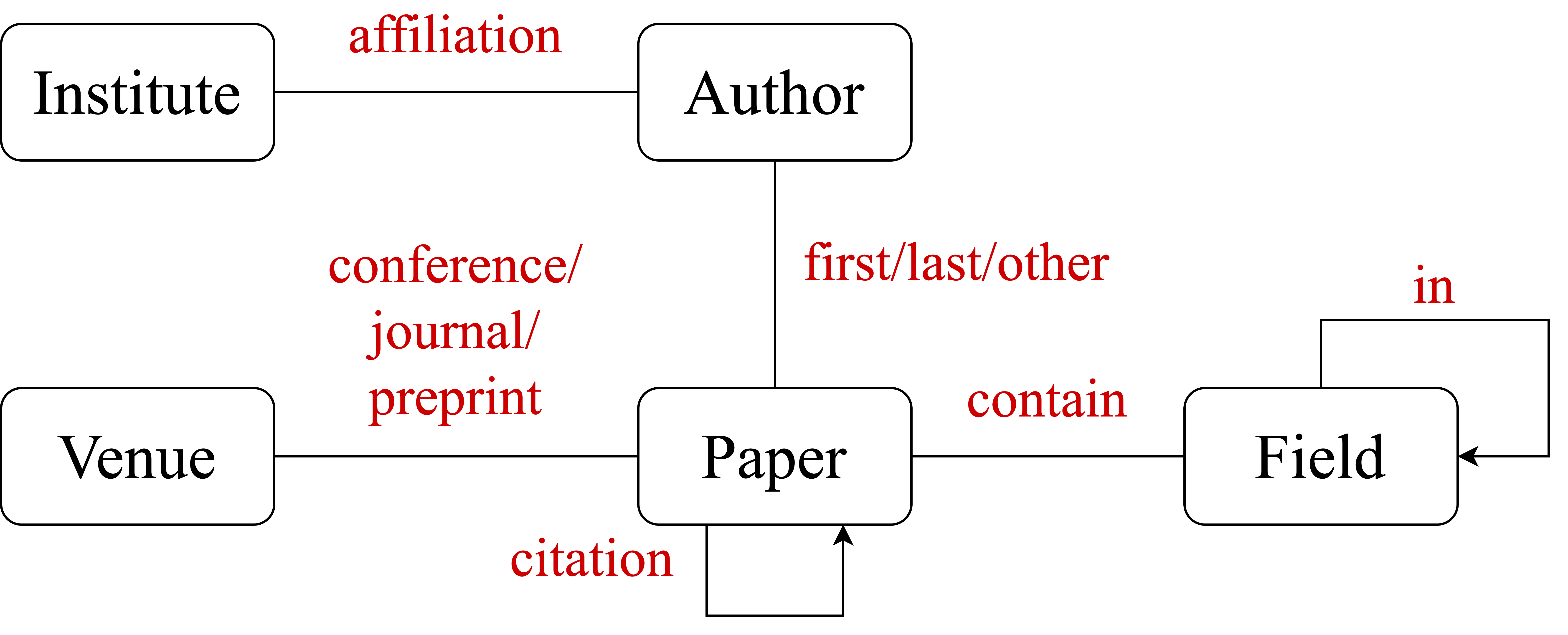
$\diamond$ Heterogeneous Graph. We use the OAG-CS dataset (Tang et al., 2008; Sinha et al., 2015), which is a publicly available heterogeneous graph containing computer science papers. The dataset contains over 1.1M nodes and 28.4M edges. In this graph, there are five node types (institute, author, venue, paper and field) and ten edge types. The “field” nodes are further categorized into six levels from L0 to L5, which are organized using a hierarchical tree. Details are shown in Figure 2.

Figure 2: Details of OAG-CS. There are 5 node types (in black) and 10 edge types (in red).

We use papers published before 2014 as the pre-training dataset (63%), papers published between 2014 (inclusive) and 2016 (inclusive) as the fine-tuning training set (20%), papers published in 2017 as the fine-tuning validation set (7%), and papers published after 2017 as the fine-tuning test set (10%). During fine-tuning, by default we only use 10% of the fine-tuning training data (i.e., 2% of the overall data) because in practice labeled data are often scarce. We consider three tasks for fine-tuning: author name disambiguation (AD), paper field classification (PF) and paper venue classification (PV). For paper field classification, we only consider L2 fields. In the experiments, we use the pre-processed graph from Hu et al. 2020b.

4.2 Baselines

We compare our method with several baselines in the experiments. For fair comparison, all the methods are trained for the same number of GPU hours.

$\diamond$ GAE (Graph Auto-Encoder, Kipf & Welling 2016) adopts an auto-encoder for unsupervised learning on graphs. In GAE, node embeddings are learnt using a GNN, and we minimize the discrepancy between the original and the reconstructed adjacency matrix.

$\diamond$ GraphSAGE (Hamilton et al., 2017) encourages embeddings of neighboring nodes to be similar. For each node, the method learns a function that generates embeddings by sampling and aggregating features from the node’s neighbors.

$\diamond$ DGI (Deep Graph Infomax, Velickovic et al. 2019) maximizes mutual information between node representations and corresponding high-level summaries of graphs. Thus, a node’s embedding summarizes a sub-graph centered around it.

$\diamond$ GPT-GNN (Hu et al., 2020b) adopts a generative pre-training objective. The method generates edges by minimizing a link prediction objective, and incorporates node features in the framework.

$\diamond$ GRACE (Graph Contrastive Representation, Zhu et al. 2020) leverages a contrastive objective. The algorithm generates two views of the same graph through node and feature corruption, and then maximize agreement of node representations in the two views.

$\diamond$ GraphCL (You et al., 2020) is another graph contrastive learning approach that adopts node and edge augmentation techniques, such as node dropping and edge perturbation.

$\diamond$ JOAO (Joint Augmentation Optimization, You et al. 2021) improves GraphCL by deigning a bi-level optimization objective to automatically and dynamically selects augmentation methods.

Table 1: Experimental results on homogeneous graphs. We report F1 averaged over 10 runs for the Reddit data and MRR over 10 runs for the product recommendation data. The best results are shown in bold.

	Reddit	Recomm.
w/o pre-train	87.3	46.3
GAE	88.5	56.7
GraphSAGE	88.0	53.0
DGI	87.7	53.3
GPT-GNN	89.6	58.6
GRACE	89.0	51.5
GraphCL	88.6	—
JOAOv2	89.1	—
DiP-GNN	90.7	60.1

Table 2: Experimental results on OAG-CS (heterogeneous). Left to right: paper-field, paper-venue, author-name-disambiguation. We report MRR over 10 runs. The best results are shown in bold.

	PF	PV	AD
w/o pre-train	32.7	19.6	60.0
GAE	40.3	24.5	62.5
GraphSAGE	37.8	22.1	62.9
DGI	38.1	22.5	63.0
GPT-GNN	41.6	25.6	63.1
GRACE	38.0	21.5	62.0
GraphCL	38.0	22.0	61.5
JOAOv2	38.6	23.5	62.8
DiP-GNN	44.1	27.7	65.6

(a) Author name disambiguation.

(b) Paper field classification.

(c) Paper venue classification.

Figure 3: Model performance vs. amount of labeled data on OAG-CS.

4.3 Main Results

In Table 1 and Table 2, w/o pre-train means direct training on the fine-tuning dataset without pre-training. Results on the Reddit dataset are F1 scores averaged over 10 runs, and results on the product recommendation graph are MRR scores averaged over 10 runs. All the performance gain have passed a hypothesis test with p-value $<0.05$.

Table 1 summarizes experimental results on the homogeneous graphs: Reddit and Recommendation. We see that pre-training indeed benefits downstream tasks. For example, performance of GNN improves by at $\geq 0.4$ F1 on Reddit (DGI) and $\geq 5.2$ MRR on Recommendation (GRACE). Also, notice that among the baselines, generative approaches (GAE and GPT-GNN) yield promising performance. On the other hand, the contrastive method (GRACE, GraphCL and JOAO) does not scale well to large graphs, e.g., the OAG-CS graph which contains 1.1M nodes and 28.4M edges. By using the proposed discriminative pre-training framework, our method significantly outperforms all the baseline approaches. For example, DiP-GNN outperforms GPT-GNN by 1.1 on Reddit and 1.5 on Recommendation.

Experimental results on the heterogeneous OAG-CS dataset are summarized in Table 2. Similar to the homogeneous graphs, notice that pre-training improves model performance by large margins. For example, pre-training improves MRR by at least 5.1, 2.5 and 2.5 on the PF, PV and AD tasks, respectively. Moreover, by using the proposed training framework, models can learn better node embeddings and yield consistently better performance compared with all the baselines.

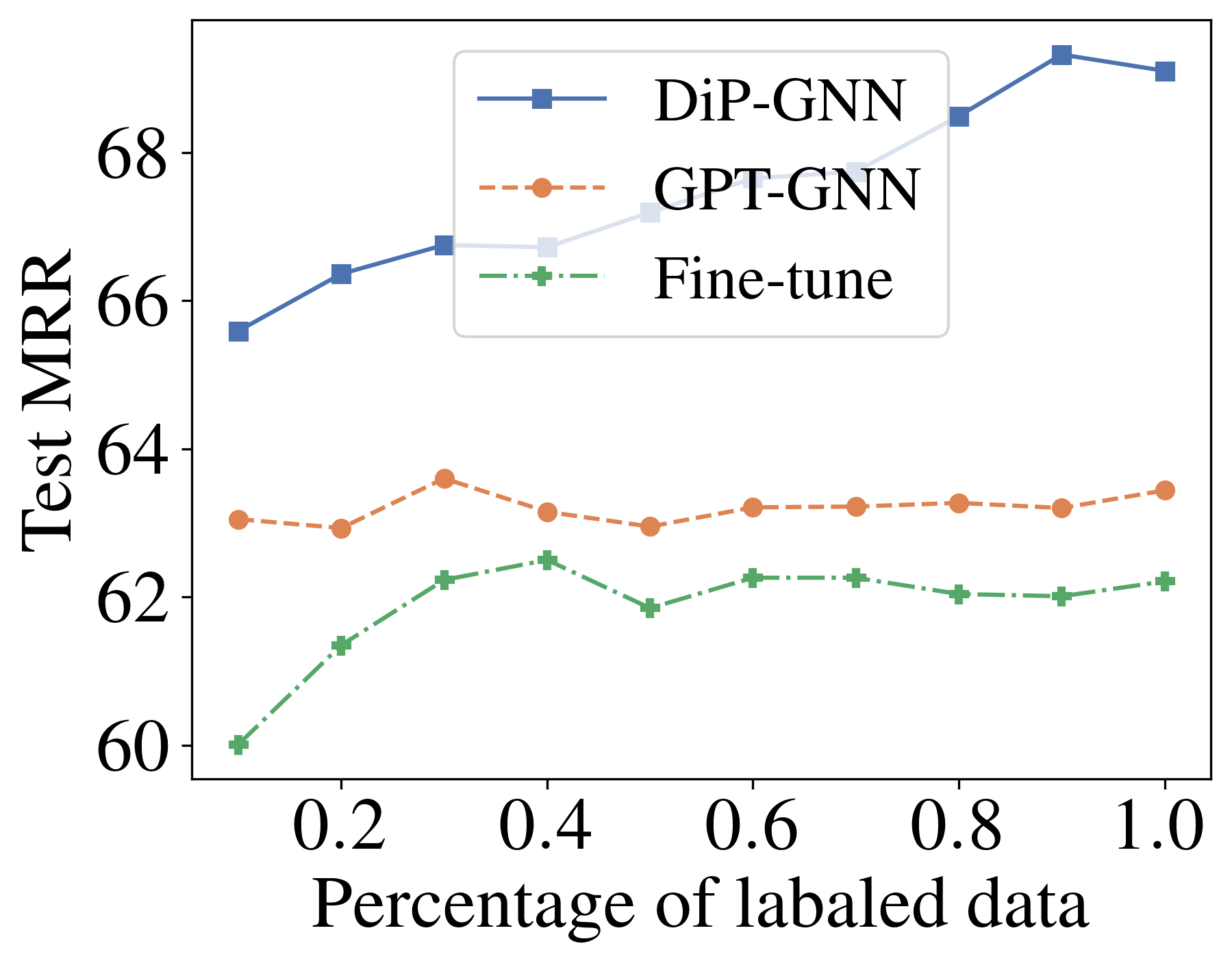
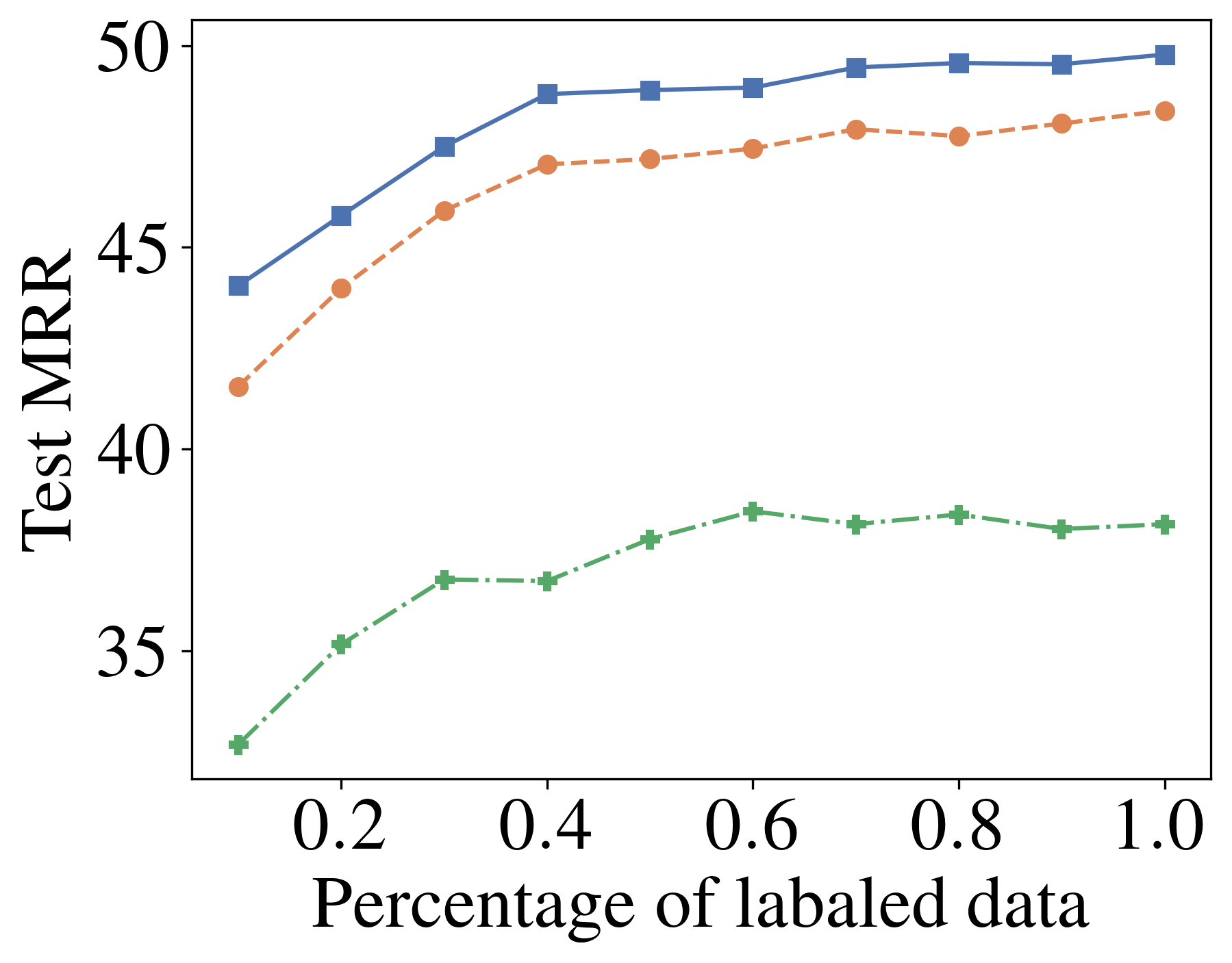
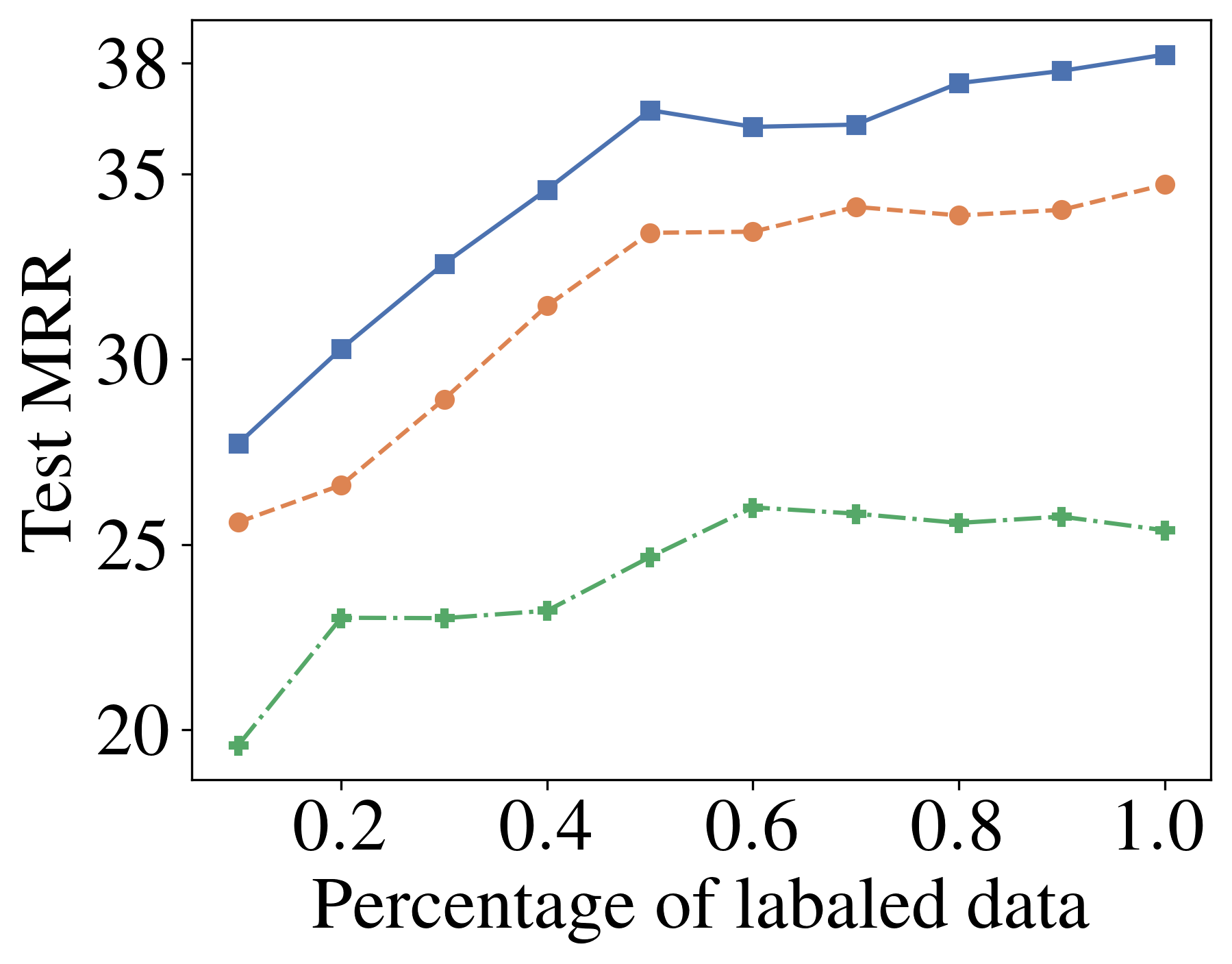
Recall that during fine-tuning on OAG-CS, we only use 10% of the labeled fine-tuning data (about 2% of the overall data). In Figure 3, we examine the effect of the amount of labeled data. We see that model performance improves when we increase the amount of labeled data. Also, notice that DiP-GNN consistently outperforms GPT-GNN in all the three tasks under all the settings.

4.4 Analysis

(a) Neg. nodes for generation.

(b) Pos. edges for discrimination.

(c) Weight of discriminator’s loss.

Figure 4: Ablation experiments on Reddit. By default, we set the number of negative nodes to 256, the factor of positive edges to 1.0, and weight of the discriminator’s loss to 20.

Table 3: Test F1 score of model variants on Reddit.

Model	F1
Edges+Features	90.7
Edges	90.4
Features	90.2
RandomEdges	89.8

Table 4: Test F1 of models with different backbone graph neural networks on Reddit.

Model	HGT	GAT
w/o pretrain	87.3	86.4
GPT-GNN	89.6	87.5
Ours	90.7	88.5

Figure 5: F1 vs. proportion of manipulated edges on Reddit.

Figure 6: Test F1 on Reddit.

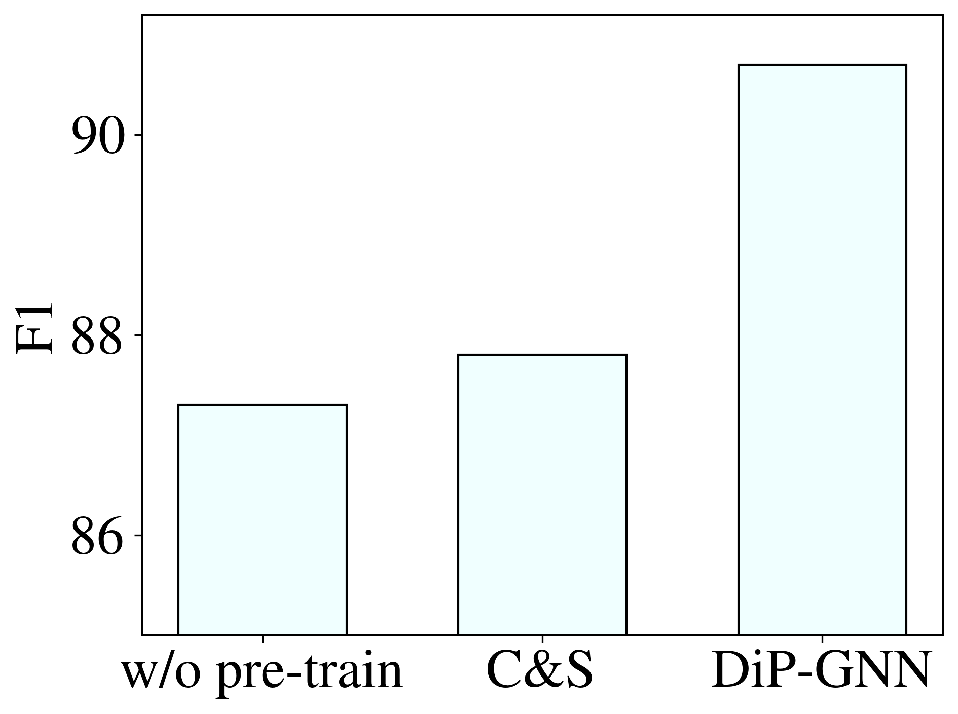
$\diamond$ Comparison with semi-supervised learning. We compare DiP-GNN with a semi-supervised learning method: C&S (Correct&Smooth, Huang et al. 2020). Figure 6 summarizes the results. We see that C&S yields a 0.5 improvement compared with the supervised learning method (i.e., w/o pre-train). However, performance of C&S is significantly lower than both DiP-GNN and other pre-training methods such as GPT-GNN.

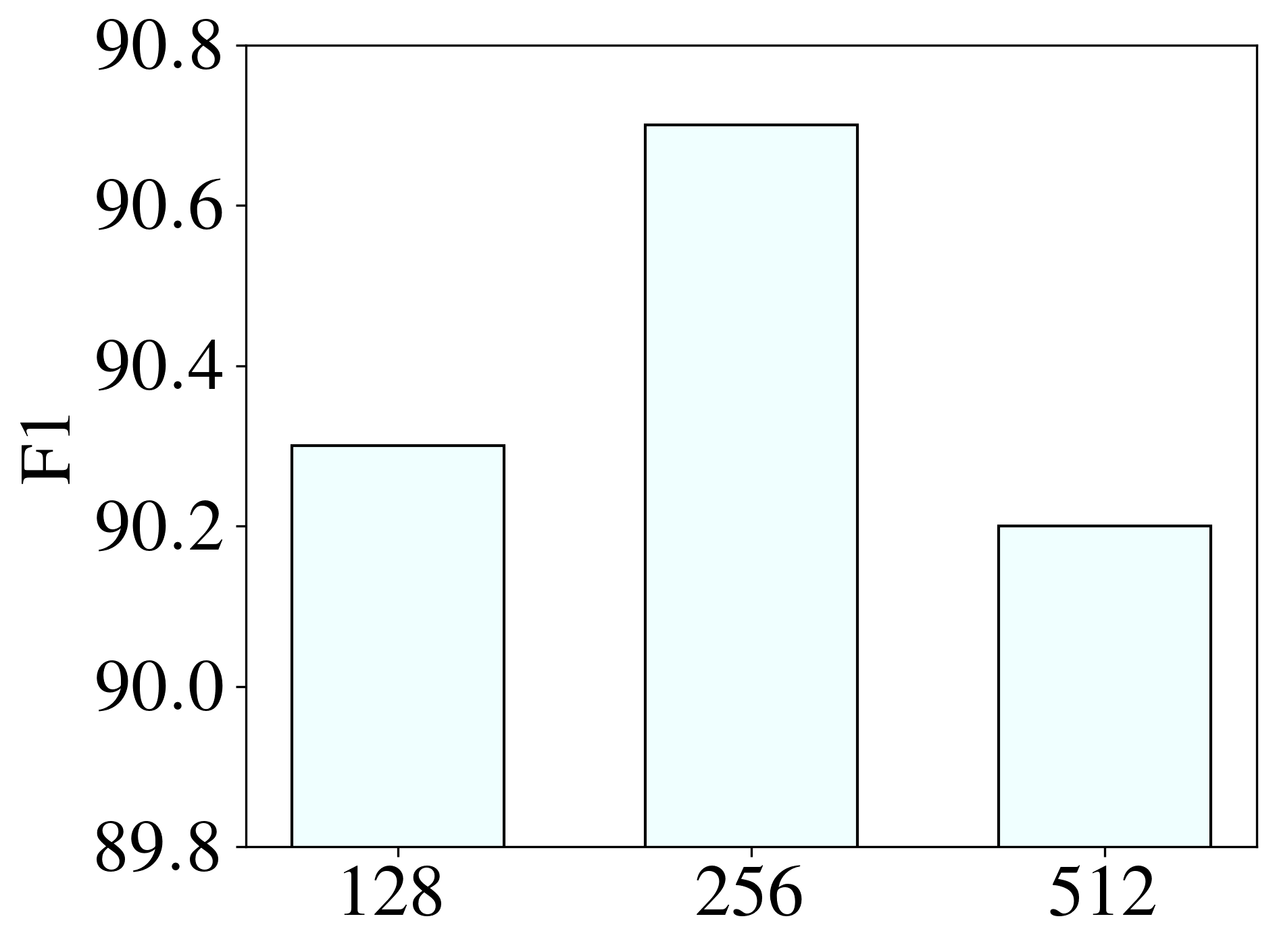
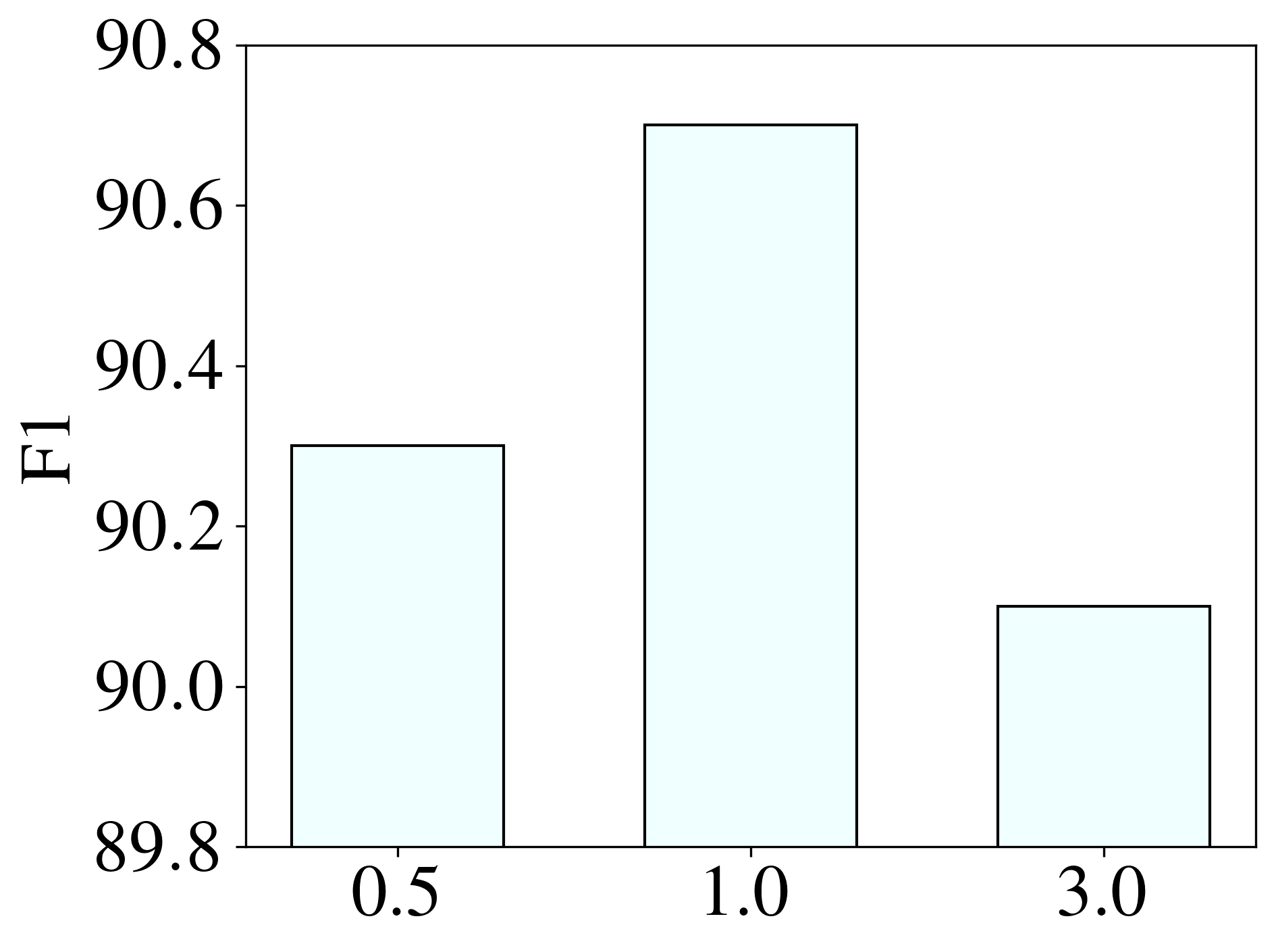
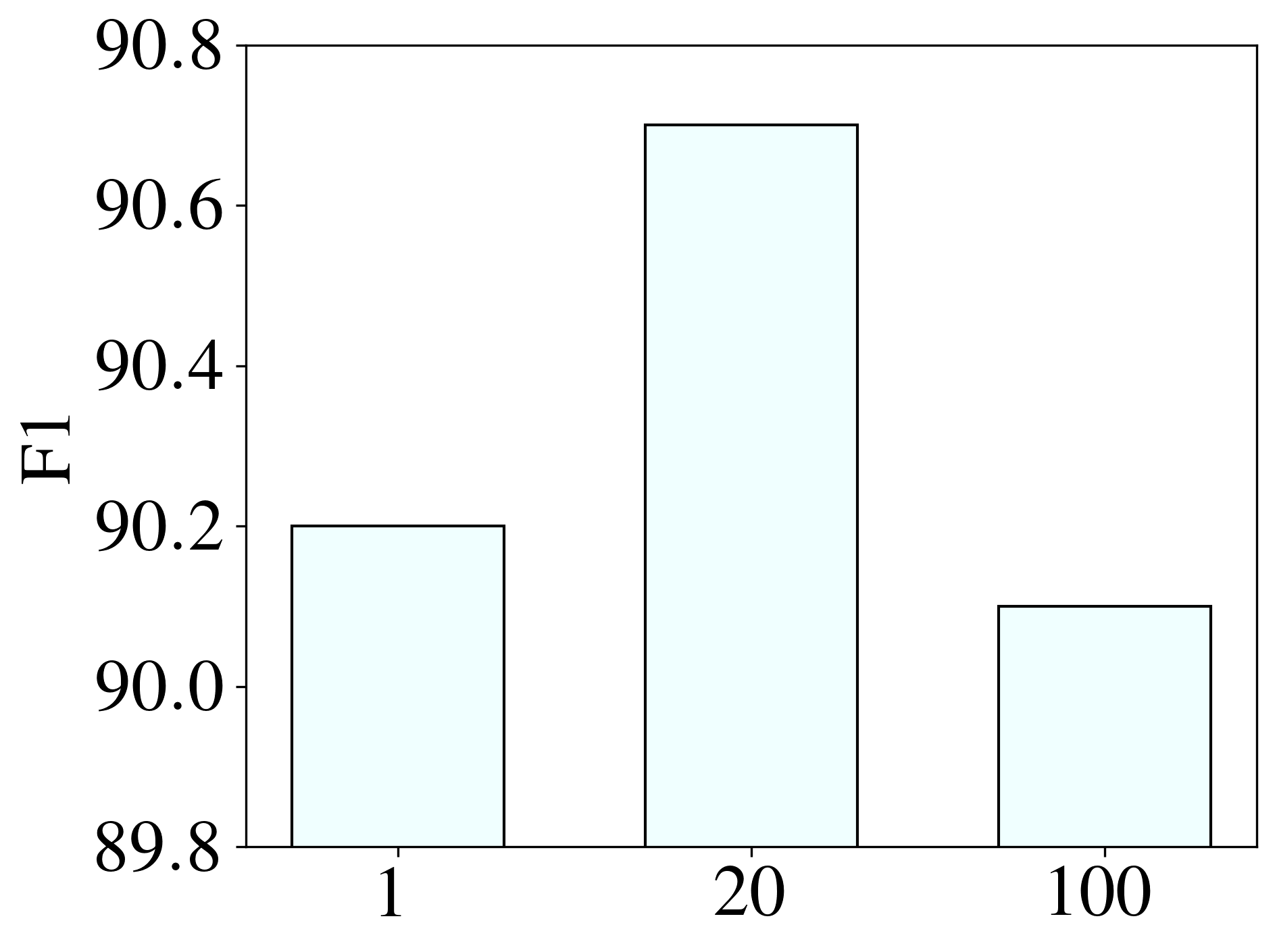
$\diamond$ Hyper-parameters. There are several hyper-parameters that we introduce in DiP-GNN: the number of negative nodes that are sampled for generating edges (Section 3.4); the number of positive edges that are sampled for the discriminator’s task (Section 3.4); and the weight of the discriminator’s loss (Eq. 3.3). Figure 4 illustrate ablation experimental results on the Reddit dataset. From the results, we see that DiP-GNN is robust to these hyper-parameters. We remark that under all the settings, ours model behaves better than the best-performing baseline (89.6 for GPT-GNN).

$\diamond$ Model variants. We also examine variants of DiP-GNN. Recall that the generator and the discriminator operate on both edges and node features. We first check the contribution of these two factors. We also investigate the scenario where edges are randomly generated, and the discriminator still seeks to find the generated edges. Table 3 summarizes results on the Reddit dataset.

We see that by only using edges, model performance drops by 0.3; and by only using node features, performance drops by 0.5. This indicates that the graph structure plays a more important role in the proposed framework than the features. Also notice that performance of RandomEdges is unsatisfactory. This is because implausible edges are generated when using a random generator, making the discriminator’s task significantly easier. We remark that performance of all the model variants is better than the best-performing baseline (89.6 for GPT-GNN).

Table 4 examines performance of our method and GPT-GNN using different backbone GNNs. Recall that by default, we use HGT (Hu et al., 2020c) as the backbone. We see that when GAT (Velickovic et al., 2018) is used, performance of DiP-GNN is still significantly better than GPT-GNN.

$\diamond$ Missing edges hurt more than wrong edges. In our pre-training framework, the generator is trained to reconstruct the masked graph, after which the reconstructed graph is fed to the discriminator. During this procedure, the graph inputted to the generator has missing edges, and the graph inputted to the discriminator has wrong edges. From Figure 5, we see that wrong edges hurt less than missing ones. For example, model performance drops by 0.7% when 50% of wrong edges are added to the original graph, and performance decreases by 1.8% when 50% of original edges are missing. This indicates that performance relies on the amount of original edges seen by the models.

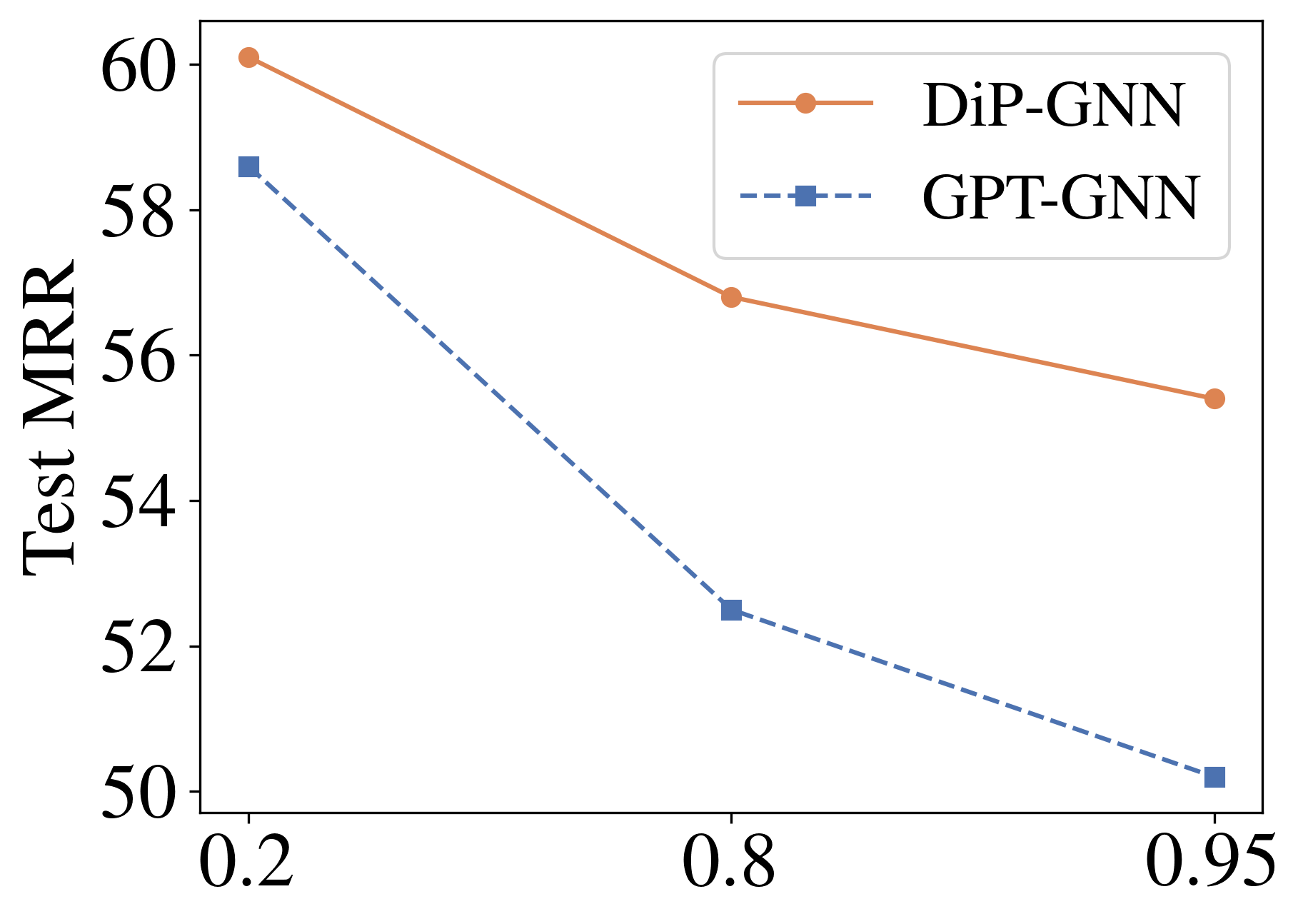
$\diamond$ Why is discriminative pre-training better? Figure 7 illustrates effect of the proportion of masked edges during pre-training. We see that when we increase the proportion from 0.2 to 0.8, performance of GPT-GNN drops by 6.1, whereas performance of DiP-GNN only drops by 3.3. This indicates that the generative pre-training method is more sensitive to the masking proportion.

Table 5 summarizes pre-training quality. First, the generative task (i.e., the generator) is more difficult than the discriminative task (i.e., the discriminator). For example, when we increase the proportion of masked edges from 20% to 80%, accuracy of the generator drops by 17% while accuracy of the discriminator only decreases by 3%. Second, the graph inputted to the discriminator better aligns with the original graph. For example, when 80% of the edges are masked, the discriminator sees 2.3 times more original edges than the generator. Therefore, the discriminative task is more advantageous because model quality relies on the number of observed original edges (Figure 5).

Figure 7: Performance vs. proportion of masked edges on product recommendation.

Table 5: Generator and discriminator performance vs. proportion of masked edges during pre-training. Coverage is the proportion of true edges inputted to the models.

Masked%	Acc		Coverage
	Gen.	Dis.	Gen.	Dis.	Ratio
20	0.50	0.87	0.80	0.90	$\times$1.13
80	0.33	0.84	0.20	0.46	$\times$2.30
95	0.20	0.80	0.05	0.24	$\times$4.80

5 Conclusion and Discussions

We propose Discriminative Pre-Training of Graph Neural Networks (DiP-GNN), where we simultaneously train a generator and a discriminator. During pre-training, we mask out some edges in the graph, and a generator is trained to recover the masked edges. Subsequently, a discriminator seeks to distinguish the generated edges from the original ones. Our framework is more advantageous than generative pre-training for two reasons: the graph inputted to the discriminator better matches the original graph; and the discriminative pre-training task better aligns with downstream node classification. We conduct extensive experiments to validate the effectiveness of DiP-GNN.

Appendix A Detailed Algorithm

Algorithm 1 is a detailed training pipeline of DiP-GNN. For graphs with vector features instead of text features, we can substitute the feature generation and discrimination modules with equations in Appendix B.

Input: Graph $\mathcal{G}_{\mathrm{full}}$; edge masking ratio; feature masking ratio; number of negative samples for edge generator; proportion of positive samples for edge discriminator $\alpha$; weight of the discriminator’s loss $\lambda$; number of training steps $T$.

for $t=0,\cdots,T-1$ do

       // Graph subsampling.

       Sample a subgraph $\mathcal{G}=(\mathcal{N},\mathcal{E})$ from $\mathcal{G}_{\mathrm{full}}$;

       // Edge generation.

       Initialize the generated edge set $\mathcal{E}_{g}=\{\}$ and the edge generation loss $\mathcal{L}_{g}^{e}=0$;

       Construct the unmasked set of edges $\mathcal{E}_{u}$ and the masked set $\mathcal{E}_{m}$ such that $\mathcal{E}=\mathcal{E}_{u}\cup\mathcal{E}_{m}$;

       Compute node embeddings using $\mathcal{E}_{u}$;

       for $e=(n_{1},n_{2})\in\mathcal{E}_{m}$ do

             Construct candidate set $\mathcal{C}$ for $n_{1}$ ($n_{2}$ is given during generation) via negative sampling;

             Generate $\widehat{e}=(\widehat{n}_{1},n_{2})$ where $\widehat{n}_{1}\in\mathcal{C}$;

             Update the generated edge set $\mathcal{E}_{g}\leftarrow\mathcal{E}_{g}\cup\{\widehat{e}\}$;

             Update the edge generation loss $\mathcal{L}_{g}^{e}$;

            

      // Text Feature generation.

       Initialize the feature generation loss $\mathcal{L}_{g}^{f}=0$;

       for $n\in\mathcal{N}$ do

             For the node’s text feature $\mathbf{x}_{n}$, mask out some of its tokens;

             Construct the generated text feature $\mathbf{x}_{n}^{\mathrm{corr}}$ using the embedding of node $n$ (computed during edge generation) and the feature generation Transformer model;

             Update the feature generation loss $\mathcal{L}_{g}^{f}$;

            

      // Edge discrimination.

       Initialize the edge discrimination loss $\mathcal{L}_{d}^{e}=0$;

       Compute node embeddings using $\mathcal{E}_{g}\cup\mathcal{E}_{u}$;

       Sample $\mathcal{E}_{u}^{d}\subset\mathcal{E}_{u}$ such that $|\mathcal{E}_{u}^{d}|=\alpha|\mathcal{E}_{g}|$;

       for $e=(n_{1},n_{2})\in\mathcal{E}_{g}\cup\mathcal{E}_{u}^{d}$ do

             Determine if $e$ is generated using the embedding of $n_{1}$ and $n_{2}$;

             Update the edge discrimination loss $\mathcal{L}_{d}^{e}$;

            

      // Text feature discrimination.

       Initialize the feature discrimination loss $\mathcal{L}_{d}^{f}=0$;

       for $n\in\mathcal{N}$ do

             For the node’s generated text feature $\mathbf{x}_{n}^{\mathrm{corr}}$, determine whether each token is generated using the embedding of node $n$ (computed during edge discrimination) and the feature discrimination Transformer model;

             Update the feature discrimination loss $\mathcal{L}_{d}^{f}$;

            

      // Model updates.

       Compute $\mathcal{L}=(\mathcal{L}_{g}^{e}+\mathcal{L}_{g}^{f})+\lambda(\mathcal{L}_{d}^{e}+\mathcal{L}_{d}^{f})$ and update the model;

      

Output: Trained discriminator ready for fine-tuning.

Algorithm 1 DiP-GNN: Discriminative Pre-training of Graph Neural Networks.

Appendix B Generation and Discrimination of Vector Features

Node features can be vectors instead of texts, e.g., the feature vector can contain topological information such as connectivity information. In this case both the generator and the discriminator are parameterized by a linear layer.

To generate feature vectors, we first randomly select some nodes $\mathcal{N}_{g}\subset\mathcal{N}$. For a node $n\in\mathcal{N}$, denote its feature vector $\mathbf{v}_{n}$, then the feature generation loss is

$$\mathcal{L}^{f}_{g}(W_{g})=\sum_{n\in N_{g}}\left|\left|\widehat{\mathbf{v}}_{n}-\mathbf{v}_{n}\right|\right|_{2}^{2},\text{ where }\widehat{\mathbf{v}}_{n}=W_{g}^{f}h_{g}(n).$$

Here $h_{g}(n)$ is the representation of node $n$ and $W_{g}^{f}$ is a trainable weight. For a node $n\in\mathcal{N}$, we construct its corred feature $\mathbf{v}^{\text{corr}}_{n}=\widehat{\mathbf{v}}_{n}$ if $n\in\mathcal{N}_{g}$ and $\mathbf{v}^{\text{corr}}_{n}=\mathbf{v}_{n}$ if $n\in\mathcal{N}\setminus\mathcal{N}_{g}$.

The discriminator’s goal is to differentiate the generated features from the original ones. Specifically, the prediction probability is

$$p(n\in\mathcal{N}_{g})=\mathrm{sigmoid}\left(W_{d}^{d}h_{d}(n)\right),$$

where $W_{d}^{f}$ is a trainable weight. We remark that the node representation $h_{d}(n)$ is computed based on the corred feature $\mathbf{v}^{\text{corr}}_{n}$. Correspondingly, the discriminator’s loss is

$$\mathcal{L}_{d}^{f}(W_{d})=\sum_{n\in\mathcal{N}}-\mathbf{1}\{n\in\mathcal{N}_{g}\}\log p(n\in\mathcal{N}_{g})-\mathbf{1}\{n\in\mathcal{N}\setminus\mathcal{N}_{g}\}\log(1-p(n\in\mathcal{N}_{g})).$$

The vector feature loss $\mathcal{L}^{f}(\theta_{g}^{e},W_{g}^{f},\theta_{d}^{e},W_{d}^{f})=\mathcal{L}_{g}^{f}(\theta_{g}^{e},W_{g}^{f})+\mathcal{L}_{d}^{f}(\theta_{d}^{e},W_{d}^{f})$ is computed similar to the text feature loss.

Appendix C Implementation and Training Details

By default, we use Heterogeneous Graph Transformer (HGT, Hu et al. 2020c) as the backbone GNN. In the experiments, the edge generator and discriminator have the same architecture, where we set the hidden dimension to 400, the number of layers to 3, and the number of attention heads to 8. For the OAG dataset which contains text features, the feature generator and discriminator employs the same architecture: a 4 layer bi-directional Transformer model, similar to BERT (Devlin et al., 2019), where we set the embedding dimension to 128 and the hidden dimension of the feed-forward neural network to 512.

For pre-training, we mask out 20% of the edges and 20% of the features (for text features we mask out 20% of the tokens). We use AdamW (Loshchilov & Hutter, 2019) as the optimizer, where we set $\beta=(0.9,0.999)$, $\epsilon=10^{-8}$, the learning rate to 0.001 and the weight decay to 0.01. We adopt a dropout ratio of 0.2 and gradient norm clipping of 0.5. For graph subsampling, we set the depth to 6 and width to 128, the same setting as Hu et al. 2020b.

For fine-tuning, we use AdamW (Loshchilov & Hutter, 2019) as the optimizer, where we set $\beta=(0.9,0.999)$, $\epsilon=10^{-6}$, and we do not use weight decay. We use the same graph subsampling setting as pre-training. The other hyper-parameters are detailed in Table 6.

Table 6: Hyper-parameters for fine-tuning tasks.

Dataset	Task	Steps	Dropout	Learning rate	Gradient clipping
Reddit	—	2400	0.3	0.0015	0.5
Recomm.	—	1600	0.1	0.0010	0.5
OAG-CS	PF	1600	0.2	0.0010	0.5
	PV	1600	0.2	0.0005	0.5
	AD	1600	0.2	0.0005	0.5

References

- Clark et al. (2020) Kevin Clark, Minh-Thang Luong, Quoc V. Le, and Christopher D. Manning. ELECTRA: pre-training text encoders as discriminators rather than generators. In 8th International Conference on Learning Representations, ICLR 2020, Addis Ababa, Ethiopia, April 26-30, 2020. OpenReview.net, 2020.
- Defferrard et al. (2016) Michaël Defferrard, Xavier Bresson, and Pierre Vandergheynst. Convolutional neural networks on graphs with fast localized spectral filtering. In Daniel D. Lee, Masashi Sugiyama, Ulrike von Luxburg, Isabelle Guyon, and Roman Garnett (eds.), Advances in Neural Information Processing Systems 29: Annual Conference on Neural Information Processing Systems 2016, December 5-10, 2016, Barcelona, Spain, pp. 3837–3845, 2016.
- Devlin et al. (2019) Jacob Devlin, Ming-Wei Chang, Kenton Lee, and Kristina Toutanova. BERT: Pre-training of deep bidirectional transformers for language understanding. In Proceedings of the 2019 Conference of the North American Chapter of the Association for Computational Linguistics: Human Language Technologies, Volume 1 (Long and Short Papers), pp. 4171–4186, Minneapolis, Minnesota, 2019. Association for Computational Linguistics. doi: 10.18653/v1/N19-1423.
- Dong et al. (2017) Yuxiao Dong, Nitesh V. Chawla, and Ananthram Swami. metapath2vec: Scalable representation learning for heterogeneous networks. In Proceedings of the 23rd ACM SIGKDD International Conference on Knowledge Discovery and Data Mining, Halifax, NS, Canada, August 13 - 17, 2017, pp. 135–144. ACM, 2017. doi: 10.1145/3097983.3098036.
- Fey & Lenssen (2019) Matthias Fey and Jan E. Lenssen. Fast graph representation learning with PyTorch Geometric. In ICLR Workshop on Representation Learning on Graphs and Manifolds, 2019.
- Goodfellow et al. (2014) Ian J. Goodfellow, Jean Pouget-Abadie, Mehdi Mirza, Bing Xu, David Warde-Farley, Sherjil Ozair, Aaron C. Courville, and Yoshua Bengio. Generative adversarial nets. In Zoubin Ghahramani, Max Welling, Corinna Cortes, Neil D. Lawrence, and Kilian Q. Weinberger (eds.), Advances in Neural Information Processing Systems 27: Annual Conference on Neural Information Processing Systems 2014, December 8-13 2014, Montreal, Quebec, Canada, pp. 2672–2680, 2014.
- Grover & Leskovec (2016) Aditya Grover and Jure Leskovec. node2vec: Scalable feature learning for networks. In Balaji Krishnapuram, Mohak Shah, Alexander J. Smola, Charu C. Aggarwal, Dou Shen, and Rajeev Rastogi (eds.), Proceedings of the 22nd ACM SIGKDD International Conference on Knowledge Discovery and Data Mining, San Francisco, CA, USA, August 13-17, 2016, pp. 855–864. ACM, 2016. doi: 10.1145/2939672.2939754.
- Hamilton et al. (2017) William L. Hamilton, Zhitao Ying, and Jure Leskovec. Inductive representation learning on large graphs. In Isabelle Guyon, Ulrike von Luxburg, Samy Bengio, Hanna M. Wallach, Rob Fergus, S. V. N. Vishwanathan, and Roman Garnett (eds.), Advances in Neural Information Processing Systems 30: Annual Conference on Neural Information Processing Systems 2017, December 4-9, 2017, Long Beach, CA, USA, pp. 1024–1034, 2017.
- Hassani & Ahmadi (2020) Kaveh Hassani and Amir Hosein Khas Ahmadi. Contrastive multi-view representation learning on graphs. In Proceedings of the 37th International Conference on Machine Learning, ICML 2020, 13-18 July 2020, Virtual Event, volume 119 of Proceedings of Machine Learning Research, pp. 4116–4126. PMLR, 2020.
- Hu et al. (2020a) Weihua Hu, Bowen Liu, Joseph Gomes, Marinka Zitnik, Percy Liang, Vijay S. Pande, and Jure Leskovec. Strategies for pre-training graph neural networks. In 8th International Conference on Learning Representations, ICLR 2020, Addis Ababa, Ethiopia, April 26-30, 2020. OpenReview.net, 2020a.
- Hu et al. (2020b) Ziniu Hu, Yuxiao Dong, Kuansan Wang, Kai-Wei Chang, and Yizhou Sun. GPT-GNN: generative pre-training of graph neural networks. In Rajesh Gupta, Yan Liu, Jiliang Tang, and B. Aditya Prakash (eds.), KDD ’20: The 26th ACM SIGKDD Conference on Knowledge Discovery and Data Mining, Virtual Event, CA, USA, August 23-27, 2020, pp. 1857–1867. ACM, 2020b.
- Hu et al. (2020c) Ziniu Hu, Yuxiao Dong, Kuansan Wang, and Yizhou Sun. Heterogeneous graph transformer. In Yennun Huang, Irwin King, Tie-Yan Liu, and Maarten van Steen (eds.), WWW ’20: The Web Conference 2020, Taipei, Taiwan, April 20-24, 2020, pp. 2704–2710. ACM / IW3C2, 2020c. doi: 10.1145/3366423.3380027.
- Huang et al. (2020) Qian Huang, Horace He, Abhay Singh, Ser-Nam Lim, and Austin R Benson. Combining label propagation and simple models out-performs graph neural networks. arXiv preprint arXiv:2010.13993, 2020.
- Kipf & Welling (2016) Thomas N Kipf and Max Welling. Variational graph auto-encoders. arXiv preprint arXiv:1611.07308, 2016.
- Kipf & Welling (2017) Thomas N. Kipf and Max Welling. Semi-supervised classification with graph convolutional networks. In 5th International Conference on Learning Representations, ICLR 2017, Toulon, France, April 24-26, 2017, Conference Track Proceedings. OpenReview.net, 2017.
- Loshchilov & Hutter (2019) Ilya Loshchilov and Frank Hutter. Decoupled weight decay regularization. In 7th International Conference on Learning Representations, ICLR 2019, New Orleans, LA, USA, May 6-9, 2019. OpenReview.net, 2019.
- Paszke et al. (2019) Adam Paszke, Sam Gross, Francisco Massa, Adam Lerer, James Bradbury, Gregory Chanan, Trevor Killeen, Zeming Lin, Natalia Gimelshein, Luca Antiga, Alban Desmaison, Andreas Köpf, Edward Yang, Zachary DeVito, Martin Raison, Alykhan Tejani, Sasank Chilamkurthy, Benoit Steiner, Lu Fang, Junjie Bai, and Soumith Chintala. Pytorch: An imperative style, high-performance deep learning library. In Hanna M. Wallach, Hugo Larochelle, Alina Beygelzimer, Florence d’Alché-Buc, Emily B. Fox, and Roman Garnett (eds.), Advances in Neural Information Processing Systems 32: Annual Conference on Neural Information Processing Systems 2019, NeurIPS 2019, December 8-14, 2019, Vancouver, BC, Canada, pp. 8024–8035, 2019.
- Perozzi et al. (2014) Bryan Perozzi, Rami Al-Rfou, and Steven Skiena. Deepwalk: online learning of social representations. In Sofus A. Macskassy, Claudia Perlich, Jure Leskovec, Wei Wang, and Rayid Ghani (eds.), The 20th ACM SIGKDD International Conference on Knowledge Discovery and Data Mining, KDD ’14, New York, NY, USA - August 24 - 27, 2014, pp. 701–710. ACM, 2014. doi: 10.1145/2623330.2623732.
- Qiu et al. (2018) Jiezhong Qiu, Yuxiao Dong, Hao Ma, Jian Li, Kuansan Wang, and Jie Tang. Network embedding as matrix factorization: Unifying deepwalk, line, pte, and node2vec. In Yi Chang, Chengxiang Zhai, Yan Liu, and Yoelle Maarek (eds.), Proceedings of the Eleventh ACM International Conference on Web Search and Data Mining, WSDM 2018, Marina Del Rey, CA, USA, February 5-9, 2018, pp. 459–467. ACM, 2018. doi: 10.1145/3159652.3159706.
- Qiu et al. (2020) Jiezhong Qiu, Qibin Chen, Yuxiao Dong, Jing Zhang, Hongxia Yang, Ming Ding, Kuansan Wang, and Jie Tang. GCC: graph contrastive coding for graph neural network pre-training. In Rajesh Gupta, Yan Liu, Jiliang Tang, and B. Aditya Prakash (eds.), KDD ’20: The 26th ACM SIGKDD Conference on Knowledge Discovery and Data Mining, Virtual Event, CA, USA, August 23-27, 2020, pp. 1150–1160. ACM, 2020.
- Schlichtkrull et al. (2018) Michael Schlichtkrull, Thomas N Kipf, Peter Bloem, Rianne van den Berg, Ivan Titov, and Max Welling. Modeling relational data with graph convolutional networks. In European semantic web conference, pp. 593–607. Springer, 2018.
- Sinha et al. (2015) Arnab Sinha, Zhihong Shen, Yang Song, Hao Ma, Darrin Eide, Bo-June Hsu, and Kuansan Wang. An overview of microsoft academic service (mas) and applications. In Proceedings of the 24th international conference on world wide web, pp. 243–246, 2015.
- Sun et al. (2020) Fan-Yun Sun, Jordan Hoffmann, Vikas Verma, and Jian Tang. Infograph: Unsupervised and semi-supervised graph-level representation learning via mutual information maximization. In 8th International Conference on Learning Representations, ICLR 2020, Addis Ababa, Ethiopia, April 26-30, 2020. OpenReview.net, 2020.
- Tang et al. (2015) Jian Tang, Meng Qu, Mingzhe Wang, Ming Zhang, Jun Yan, and Qiaozhu Mei. LINE: large-scale information network embedding. In Aldo Gangemi, Stefano Leonardi, and Alessandro Panconesi (eds.), Proceedings of the 24th International Conference on World Wide Web, WWW 2015, Florence, Italy, May 18-22, 2015, pp. 1067–1077. ACM, 2015. doi: 10.1145/2736277.2741093.
- Tang et al. (2008) Jie Tang, Jing Zhang, Limin Yao, Juanzi Li, Li Zhang, and Zhong Su. Arnetminer: extraction and mining of academic social networks. In Proceedings of the 14th ACM SIGKDD international conference on Knowledge discovery and data mining, pp. 990–998, 2008.
- Vaswani et al. (2017) Ashish Vaswani, Noam Shazeer, Niki Parmar, Jakob Uszkoreit, Llion Jones, Aidan N. Gomez, Lukasz Kaiser, and Illia Polosukhin. Attention is all you need. In Isabelle Guyon, Ulrike von Luxburg, Samy Bengio, Hanna M. Wallach, Rob Fergus, S. V. N. Vishwanathan, and Roman Garnett (eds.), Advances in Neural Information Processing Systems 30: Annual Conference on Neural Information Processing Systems 2017, December 4-9, 2017, Long Beach, CA, USA, pp. 5998–6008, 2017.
- Velickovic et al. (2018) Petar Velickovic, Guillem Cucurull, Arantxa Casanova, Adriana Romero, Pietro Liò, and Yoshua Bengio. Graph attention networks. In 6th International Conference on Learning Representations, ICLR 2018, Vancouver, BC, Canada, April 30 - May 3, 2018, Conference Track Proceedings. OpenReview.net, 2018.
- Velickovic et al. (2019) Petar Velickovic, William Fedus, William L. Hamilton, Pietro Liò, Yoshua Bengio, and R. Devon Hjelm. Deep graph infomax. In 7th International Conference on Learning Representations, ICLR 2019, New Orleans, LA, USA, May 6-9, 2019. OpenReview.net, 2019.
- Wang et al. (2018) Hongwei Wang, Jia Wang, Jialin Wang, Miao Zhao, Weinan Zhang, Fuzheng Zhang, Xing Xie, and Minyi Guo. Graphgan: Graph representation learning with generative adversarial nets. In Sheila A. McIlraith and Kilian Q. Weinberger (eds.), Proceedings of the Thirty-Second AAAI Conference on Artificial Intelligence, (AAAI-18), the 30th innovative Applications of Artificial Intelligence (IAAI-18), and the 8th AAAI Symposium on Educational Advances in Artificial Intelligence (EAAI-18), New Orleans, Louisiana, USA, February 2-7, 2018, pp. 2508–2515. AAAI Press, 2018.
- Wang et al. (2019) Xiao Wang, Houye Ji, Chuan Shi, Bai Wang, Yanfang Ye, Peng Cui, and Philip S. Yu. Heterogeneous graph attention network. In Ling Liu, Ryen W. White, Amin Mantrach, Fabrizio Silvestri, Julian J. McAuley, Ricardo Baeza-Yates, and Leila Zia (eds.), The World Wide Web Conference, WWW 2019, San Francisco, CA, USA, May 13-17, 2019, pp. 2022–2032. ACM, 2019. doi: 10.1145/3308558.3313562.
- Xu et al. (2019) Keyulu Xu, Weihua Hu, Jure Leskovec, and Stefanie Jegelka. How powerful are graph neural networks? In 7th International Conference on Learning Representations, ICLR 2019, New Orleans, LA, USA, May 6-9, 2019. OpenReview.net, 2019.
- Ying et al. (2018) Rex Ying, Ruining He, Kaifeng Chen, Pong Eksombatchai, William L. Hamilton, and Jure Leskovec. Graph convolutional neural networks for web-scale recommender systems. In Yike Guo and Faisal Farooq (eds.), Proceedings of the 24th ACM SIGKDD International Conference on Knowledge Discovery & Data Mining, KDD 2018, London, UK, August 19-23, 2018, pp. 974–983. ACM, 2018. doi: 10.1145/3219819.3219890.
- You et al. (2020) Yuning You, Tianlong Chen, Yongduo Sui, Ting Chen, Zhangyang Wang, and Yang Shen. Graph contrastive learning with augmentations. Advances in Neural Information Processing Systems, 33:5812–5823, 2020.
- You et al. (2021) Yuning You, Tianlong Chen, Yang Shen, and Zhangyang Wang. Graph contrastive learning automated. In International Conference on Machine Learning, pp. 12121–12132. PMLR, 2021.
- Zhang et al. (2019) Chuxu Zhang, Dongjin Song, Chao Huang, Ananthram Swami, and Nitesh V. Chawla. Heterogeneous graph neural network. In Ankur Teredesai, Vipin Kumar, Ying Li, Rómer Rosales, Evimaria Terzi, and George Karypis (eds.), Proceedings of the 25th ACM SIGKDD International Conference on Knowledge Discovery & Data Mining, KDD 2019, Anchorage, AK, USA, August 4-8, 2019, pp. 793–803. ACM, 2019. doi: 10.1145/3292500.3330961.
- Zhu et al. (2020) Yanqiao Zhu, Yichen Xu, Feng Yu, Qiang Liu, Shu Wu, and Liang Wang. Deep graph contrastive representation learning. arXiv preprint arXiv:2006.04131, 2020.
- Zhu et al. (2021) Yanqiao Zhu, Yichen Xu, Feng Yu, Qiang Liu, Shu Wu, and Liang Wang. Graph contrastive learning with adaptive augmentation. In Proceedings of the Web Conference 2021, pp. 2069–2080, 2021.
- Zou et al. (2019) Difan Zou, Ziniu Hu, Yewen Wang, Song Jiang, Yizhou Sun, and Quanquan Gu. Layer-dependent importance sampling for training deep and large graph convolutional networks. In Hanna M. Wallach, Hugo Larochelle, Alina Beygelzimer, Florence d’Alché-Buc, Emily B. Fox, and Roman Garnett (eds.), Advances in Neural Information Processing Systems 32: Annual Conference on Neural Information Processing Systems 2019, NeurIPS 2019, December 8-14, 2019, Vancouver, BC, Canada, pp. 11247–11256, 2019.