Euler scheme for approximation of solution of nonlinear ODEs under inexact information

Abstract.

We investigate error of the Euler scheme in the case when the right-hand side function of the underlying ODE satisfies nonstandard assumptions such as local one-sided Lipschitz condition and local Hölder continuity. Moreover, we assume two cases in regards to information availability: exact and noisy with respect to the right-hand side function. Optimality analysis of the Euler scheme is also provided. Finally, we present the results of some numerical experiments.

Mathematics Subject Classification: 65L05, 65L70

1. Introduction

In this paper we investigate error of the Euler scheme for the following initial-value problems

$$\left\{\begin{array}[]{ll}z^{\prime}(t)=g(t,z(t)),&t\in[a,b],\\ z(a)=\xi,\end{array}\right.$$ (1.3)

where $-\infty<a<b<+\infty$, $\xi\in\mathbb{R}^{d}$ and a right-hand side function $g:[a,b]\times\mathbb{R}^{d}\to\mathbb{R}^{d}$, $d\in\mathbb{Z}_{+}$. Comparing to the classical assumptions such as global Lipschitz condition we assume that the right-hand side function $g$ is continuous and of at most linear growth, but it satisfies the one-sided Lipschitz condition together with the Hölder condition only locally.

The numerical approximation of solutions of ordinary differential equations (ODEs) has drawn the attention of numerous scientists [4, 5, 8, 10, 11, 13]. Furthermore, solving ODE problems with noisy information was studied in [2, 3, 14, 16, 17, 25, 26, 29, 31, 32]. Also, approximation of the solutions of partial differential equations or stochastic differential equations with both exact and inexact information was a subject of extensive study, [1, 21, 22, 33, 35, 36] and [20, 24, 19, 27, 28] respectively. Nevertheless, when it comes to the nonstandard assumptions about the right-hand side function of the initial-value problem, only the existence and uniqueness of the solutions were examined, see [9]. There is a gap in the literature about numerical methods for such cases under nonstandard assumptions.

If we take a closer look at the computation on a digital computer, we quickly conclude that the computer uses only a finite set of numbers because of the finite memory. So all computer calculations are burdened with errors, e.g., from rounding. Also, the novel CPUs and GPUs have an option to speed up the computations when there is lower precision of the processed numbers. From the mathematical point of view, lowering the precision can be interpreted as adding noisy information with the control for the relative error of the noise. Hence, all the applied numerical methods should have a strict error analysis with noisy information setting.

In this paper, we deal with nonstandard assumptions about the right-hand side function $g$, and we allow both exact and inexact information about the initial value $\xi$ and values of the right-hand side function $g$. We changed a bit of assumptions from the auxiliary ordinary differential equation in [7] where we assume locally Hölder continuity and global one-sided Lipschitz conditions. Now we locally consider Hölder continuity and one-sided Lipschitz condition only in a certain neighborhood. This weakening of the assumptions was caused by the necessity that came from a phase change model of metallic materials [6, 7].

According to our best knowledge, there is a lack of literature on numerical methods of initial-value problems under nonstandard assumptions with noisy information. We focus on the most basic explicit Euler scheme. We believe that this paper might be helpful for further research on implicit numerical methods, higher-order methods, or even numerical methods for delay differential equations with noisy information under nonstandard assumptions on the right-hand side function.

To do so, we start with an error analysis for the classical explicit Euler scheme under nonstandard assumptions for the right-hand side function $g$ mentioned before, i.e., local Hölder continuity and one-sided Lipschitz condition (Theorem 3.1). Next, we introduce a corruption for the right-hand side function and then we perform an error analysis for the Euler scheme (Theorem 4.1). In both cases, we show the dependence of the error on Hölder exponents of the right-hand side function. Furthermore, we establish lower bounds for all algorithms based on exact and inexact information in the certain class of right-hand side functions (Proposition 5.1 and Proposition 5.2 respectively). Consequently, we can provide a result concerning the optimality of the Euler scheme in a particular case (Theorem 5.3). The final contribution is performing numerical experiments to confirm our theoretical results.

The paper is organized as follows. The problem posing with the nonstandard assumptions is given in Section 2. Section 3 on exact information includes a definition of the Euler scheme and a result on the upper bound of the error of this scheme under mentioned nonstandard assumptions. The detailed meaning of the noise, which corrupts values of right-hand side function as well as initial value, is explained in Section 4, along with the definition of the Euler scheme in case of inexact information and the upper bound of the Euler scheme’s error with available only noisy standard information about the right-hand side function. Finally, Section 5 contains the definition of the setting in the spirit of information-based complexity (see [34]), the lower bounds of the Euler scheme, and the optimality of this scheme as the main result of this paper. Section 6 is dedicated to numerical experiments performed using our implementation of the Euler scheme. Last but not least, we put all the auxiliary results (including, a proof of the existence and uniqueness of the solutions of (1.3)) in the Appendix.

2. Preliminaries

For $x,y\in\mathbb{R}^{d}$ we take $\displaystyle{\langle x,y\rangle=\sum\limits_{k=1}^{d}x_{k}y_{k}}$ and $\|x\|=\langle x,x\rangle^{1/2}$. For $R\in[0,+\infty]$ and $x\in\mathbb{R}^{d}$, we denote by $B_{x}(R)=\{y\in\mathbb{R}^{d}\ |\ \|y-x\|\leq R\}$. Of course $B_{x}(+\infty)=\mathbb{R}^{d}$. Moreover, for $H\in\mathbb{R}$ we denote by $H^{+}=\max\{0,H\}$. Additionally, by $U\in\textrm{comp}(\mathbb{R}^{d})$ we mean that $U\subset\mathbb{R}^{d}$ is a compact set.

We assume that the right-hand side function $g:[a,b]\times\mathbb{R}^{d}\to\mathbb{R}^{d}$ satisfies the following conditions:

• $g\in C([a,b]\times\mathbb{R}^{d};\mathbb{R}^{d})$.

• There exists $K\in(0,+\infty)$ such that for all $(t,y)\in[a,b]\times\mathbb{R}^{d}$

  $$\|g(t,y)\|\leq K(1+\|y\|).$$

• For every $U\in\textrm{comp}(\mathbb{R}^{d})$ there exists $H_{U}\in\mathbb{R}$ such that for all $t\in[a,b]$, $y_{1},y_{2}\in U$

  $$\langle y_{1}-y_{2},g(t,y_{1})-g(t,y_{2})\rangle\leq H_{U}\|y_{1}-y_{2}\|^{2}.$$

• There exist $\alpha,\beta\in(0,1]$ such that for every $U\in\textrm{comp}(\mathbb{R}^{d})$ there exists $L_{U}\in(0,\infty)$ such that for all $t_{1},t_{2}\in[a,b]$, $y_{1},y_{2}\in U$

  $$\|g(t_{1},y_{1})-g(t_{2},y_{2})\|\leq L_{U}\Bigl{(}|t_{1}-t_{2}|^{\alpha}+\|y_{1}-y_{2}\|^{\beta}\Bigr{)}.$$

The assumption (G2) is the classical global linear growth condition. However, instead of a global Lipschitz condition, we assume that the right-hand side function $g$ locally satisfies one-sided Lipschiz assumption (G3). It follows from Lemma 7.2 that under the assumptions (G1)-(G3) the equation (1.3) has a unique solution $z\in C^{1}([a,b];\mathbb{R}^{d})$. The additional assumption (G4), called the $(\alpha,\beta)$-local Hölder condition, is needed to obtain an upper error bound for the Euler scheme that depends on $(\alpha,\beta)$. We stress that under the assumptions (G1)-(G4) the right-hand side function might be highly nonlinear, see, for example, Section  6.

In the next section, we investigate the error of the classical Euler scheme under such nonstandard assumptions. Furthermore, we consider the cases where exact and inexact information about the right-hand side function $g$ is available.

3. Euler scheme under exact information

Let $n\in\mathbb{Z}_{+}$, $t_{k}=a+kh$ for $k=0,1,\dots,n$ where $h=\frac{b-a}{n}$. The Euler scheme is defined as follows

$$\left\{\begin{array}[]{ll}y_{0}=\xi,\\ y_{k+1}=y_{k}+h\cdot g(t_{k},y_{k})\quad\hbox{for}&k=0,1,\dots,n-1,\end{array}\right.$$ (3.3)

The approximation of $z=z(t)$ in $[a,b]$ is given by a piecewise linear function $l_{n}:[a,b]\to\mathbb{R}^{d}$, defined in the following way

$$l_{n}(t)=l_{k,n}(t)\ \hbox{for}\ t\in[t_{k},t_{k+1}],\ k=0,1,\ldots,n-1,$$ (3.4)

where

$$l_{k,n}(t)=y_{k}+(t-t_{k})\cdot g(t_{k},y_{k}).$$ (3.5)

The aim of this section is to prove the following result.

Theorem 3.1.

Let $\xi\in\mathbb{R}^{d}$ and let us assume that $g$ satisfies (G1)-(G4). Then there exists $\bar{C}_{1}\in[0,\infty)$ such that for all $n\in\mathbb{N}$

$$\sup\limits_{a\leq t\leq b}\|z(t)-l_{n}(t)\|\leq\bar{C}_{1}(1+\|\xi\|)(h^{\alpha}+h^{\beta}).$$ (3.6)

Proof.

By the assumption (G2) we have that for all $k=0,1,\ldots,n-1$

$$\|y_{k+1}\|\leq\|y_{k}\|+h\|g(t_{k},y_{k})\|\leq(1+hK)\|y_{k}\|+hK.$$

Hence, by the discrete version of Gronwall’s lemma we get that for all $k=0,1,\ldots,n$ that

$$\|y_{k}\|\leq(1+Kh)^{k}\|\xi\|+(1+Kh)^{k}-1\leq e^{K(b-a)}(1+\|\xi\|),$$ (3.7)

and therefore

$$\max_{n\in\mathbb{Z}_{+}}\max_{0\leq k\leq n}\|y_{k}\|\leq C_{1}(1+\|\xi\|),$$ (3.8)

where $C_{1}=C_{1}(a,b,K)=e^{K(b-a)}$. Note that $C_{1}\leq C_{0}$, where $C_{0}$ is defined in Lemma 7.2. Now for $k=0,1,\ldots,n-1$ we consider the following local ODE

$$z_{k}^{\prime}(t)=g(t,z_{k}(t)),\quad t\in[t_{k},t_{k+1}],\quad z_{k}(t_{k})=y_{k}.$$ (3.9)

By Lemma 7.2 there exists a unique solution $z_{k}:[t_{k},t_{k+1}]\to\mathbb{R}^{d}$ of (3.9). From the assumption (G2) and by (3.8) we get for all $t\in[t_{k},t_{k+1}]$, $k=0,1,\ldots,n-1$ that

$$\|z_{k}(t)\|\leq e^{K(b-a)}(1+\|\xi\|)+K(b-a)+K\int\limits_{t_{k}}^{t}\|z_{k}(s)\|ds,$$ (3.10)

and, by the Gronwall’s lemma,

$$\max_{n\in\mathbb{Z}_{+}}\max_{k=0,1,\dots,n-1}\sup_{t_{k}\leq t\leq t_{k+1}}\|z_{k}(t)\|\leq C_{2}(\|\xi\|+1),$$ (3.11)

where $C_{2}=C_{2}(a,b,K)=e^{K(b-a)}[e^{K(b-a)}+K(b-a)]$. We have $C_{0}\leq C_{2}$. Moreover, by (G2) and (3.11) we have for $t\in[t_{k},t_{k+1}]$, $k=0,1,\ldots,n-1$

$$\|z_{k}(t)-y_{k}\|\leq hK\Bigl{(}1+\sup\limits_{t_{k}\leq t\leq t_{k+1}}\|z_{k}(t)\|\Bigr{)}\leq hC_{3}(1+\|\xi\|),$$ (3.12)

where $C_{3}=C_{3}(a,b,K)=K(1+C_{2})=K(1+e^{K(b-a)}[e^{K(b-a)}+K(b-a)])$. Therefore, by (3.8), (3.11), (7.1) we have

$$y_{k},z_{k}(t),z(t)\in B_{0}(C_{2}(1+\|\xi\|))$$ (3.13)

for all $t\in[t_{k},t_{k+1}]$, $k=0,1,\ldots,n-1$, $n\in\mathbb{N}$. This and (G4) imply that for $U=B_{0}(C_{2}(1+\|\xi\|))$ there exists $L_{1}\in(0,+\infty)$ such that for all $k=0,1,\ldots,n-1$, $n\in\mathbb{N}$

$$\|z_{k}(t_{k+1})-y_{k+1}\|\leq\int_{t_{k}}^{t_{k+1}}\|g(s,z_{k}(s))-g(t_{k},y_{k})\|ds$$

$$\leq L_{1}\int_{t_{k}}^{t_{k+1}}(|s-t_{k}|^{\alpha}+\|z_{k}(s)-y_{k}\|^{\beta})ds\leq L_{1}C_{4}(1+\|\xi\|)h(h^{\alpha}+h^{\beta}),$$ (3.14)

where $C_{4}=C_{4}(a,b,K,\beta)=\max\{1,2C_{3}^{\beta}\}$. (We have also used the fact that $(1+x)^{\beta}\leq 2+x\leq 2(1+x)$ for all $x\geq 0$, $\beta\in(0,1]$.) Furthermore, for $k=0,1,\dots,n-1$ we have

$$\|z(t_{k+1})-y_{k+1}\|\leq\|z(t_{k+1})-z_{k}(t_{k+1})\|+\|z_{k}(t_{k+1})-y_{k+1}\|,$$ (3.15)

and for $t\in[t_{k},t_{k+1}]$, $k=0,1,\ldots,n-1$ it holds that

$$\frac{d}{dt}\|z(t)-z_{k}(t)\|^{2}=2\langle z(t)-z_{k}(t),g(t,z(t))-g(t,z_{k}(t))\rangle.$$ (3.16)

Therefore, by (G3) applied to $U=B_{0}(C_{2}(1+\|\xi\|))$ we receive that there exists $H_{1}\in\mathbb{R}$ such that

$$\frac{d}{dt}\|z(t)-z_{k}(t)\|^{2}\leq 2H_{1}\|z(t)-z_{k}(t)\|^{2}\\ \leq 2H_{1}^{+}\|z(t)-z_{k}(t)\|^{2}$$

for all $t\in[t_{k},t_{k+1}]$, $k=0,1,\ldots,n-1$, $n\in\mathbb{N}$. Since $z_{k}(t_{k})=y_{k}$, we get

$$\|z(t)-z_{k}(t)\|^{2}\leq\|z(t_{k})-y_{k}\|^{2}+2H^{+}_{1}\int\limits_{t_{k}}^{t}\|z(s)-z_{k}(s)\|^{2}ds,$$ (3.17)

for $t\in[t_{k},t_{k+1}]$ and, by the Gronwall’s lemma,

$$\|z(t)-z_{k}(t)\|\leq e^{H_{1}^{+}(t-t_{k})}\|z(t_{k})-y_{k}\|.$$ (3.18)

Combining (3), (3.15), (3.18) we receive for $k=0,1,\ldots,n-1$

$$\|z(t_{k+1})-y_{k+1}\|\leq e^{H_{1}^{+}h}\|z(t_{k})-y_{k}\|+L_{1}C_{4}(1+\|\xi\|)h(h^{\alpha}+h^{\beta}).$$ (3.19)

Denoting by $e_{k}=z(t_{k})-y_{k}$ we arrive at

$$\|e_{k+1}\|\leq e^{H_{1}^{+}h}\|e_{k}\|+L_{1}C_{4}(1+\|\xi\|)h(h^{\alpha}+h^{\beta}),$$

with $e_{0}=z(a)-y_{0}=0$. If $H_{1}^{+}>0$ then by Gronwall’s lemma we obtain

$$\|e_{k}\|\leq\frac{e^{H_{1}^{+}(b-a)}-1}{H_{1}^{+}}L_{1}C_{4}(1+\|\xi\|)(h^{\alpha}+h^{\beta}),$$ (3.20)

for $k=0,1,\ldots,n$, where $C_{4}=C_{4}(a,b,K,\beta)$. In the particular case, when $H_{1}^{+}=0$ we simply have that for $k=0,1,\ldots,n$

$$\|e_{k}\|\leq kL_{1}C_{4}(1+\|\xi\|)(h^{\alpha}+h^{\beta})\leq(b-a)L_{1}C_{4}(1+\|\xi\|)(h^{\alpha}+h^{\beta}).$$ (3.21)

For $t\in[t_{k},t_{k+1}]$, $k=0,1,\ldots,n$ we have by (3.18) that

$$\|z(t)-l_{n}(t)\|=\|z(t)-l_{k,n}(t)\|\leq\|z(t)-z_{k}(t)\|+\|z_{k}(t)-l_{k,n}(t)\|$$

$$\leq e^{H_{1}^{+}h}\|e_{k}\|+\|z_{k}(t)-l_{k,n}(t)\|,$$ (3.22)

where by (3)

$$\|z_{k}(t)-l_{k,n}(t)\|\leq\int\limits_{t_{k}}^{t_{k+1}}\|g(s,z_{k}(s))-g(t_{k},y_{k})\|ds\leq L_{1}C_{4}(1+\|\xi\|)h(h^{\alpha}+h^{\beta}).$$ (3.23)

Combining (3), (3.23), (3.20), (3.21) we get the thesis. ∎

4. Euler scheme under noisy information

In this section we show the upper bound for the error of the Euler scheme in the case of inexact information. Namely, we consider the corrupted right-hand side functions of the following form

$$\tilde{g}(t,y)=g(t,y)+\delta_{g}(t,y),\quad(t,y)\in[a,b]\times\mathbb{R}^{d},$$ (4.1)

where $\delta_{g}:[a,b]\times\mathbb{R}^{d}\rightarrow\mathbb{R}^{d}$ is a corrupting function that is Borel measurable and

$$\|\delta_{g}(t,y)\|\leq\delta(1+\|y\|)$$ (4.2)

for all $(t,y)\in[a,b]\times\mathbb{R}^{d}$ and $\delta\in[0,1]$. We refer to $\delta$ as to precision parameter.

In the case of inexact evaluations of $g$, the Euler scheme has the following form

$$\left\{\begin{array}[]{ll}\tilde{y}_{0}=\tilde{\xi},\\ \tilde{y}_{k+1}=\tilde{y}_{k}+h\cdot\tilde{g}(t_{k},\tilde{y}_{k}),&k=0,1,\dots,n-1,\end{array}\right.$$ (4.5)

where $\tilde{\xi}\in B_{\xi}(\delta)$. The approximation of $z=z(t)$ in $[a,b]$ is given by a piecewise linear function $\tilde{l}_{n}:[a,b]\to\mathbb{R}^{d}$, defined as

$$\tilde{l}_{n}(t)=\tilde{l}_{k,n}(t)\ \hbox{for}\ t\in[t_{k},t_{k+1}],\ k=0,1,\ldots,n-1,$$ (4.6)

where

$$\tilde{l}_{k,n}(t)=\tilde{y}_{k}+(t-t_{k})\cdot\tilde{g}(t_{k},\tilde{y}_{k}).$$ (4.7)

Of course when the information is exact (i.e., $\delta=0$) then $\tilde{y}_{k}=y_{k}$ for $k=0,1,\ldots,n$, and $l_{n}\equiv\tilde{l}_{n}$. Moreover, the Euler algorithm $\tilde{l}_{n}$ uses $n$ (noisy) evaluations of $\tilde{g}$.

In the theorem below we show the upper error bound for the Euler scheme in the case of inexact information about the function $g$. We stress that we have different bounds in the local Lipschitz case ($\beta=1$) and in the local Hölder case ($\beta\in(0,1)$). This is due to the fact that locally Lipschitz continuous function (i.e. $\beta=1$ in (G4)) satisfies also locally one-sided Lipschitz condition (G3). This is not the case when $g$ is only locally Hölder continuous. We stress that the condition (G3) is crucial for obtaining the upper error bound in the case when $\beta\in(0,1)$, see also Remark 4.2.

Theorem 4.1.

Let $\xi\in\mathbb{R}^{d}$, let $g$ satisfy (G1)-(G4), and let $\delta_{g}$ be a Borel measurable corrupting function satisfying (4.2). Then there exists $\bar{C}_{2}\in[0,\infty)$ such that for all $n\in\mathbb{N}$, $n\geq\lceil 2(b-a)\rceil+1$, $\delta\in[0,1]$, $\tilde{\xi}\in B_{\xi}(\delta)$ the following holds:

• if $\beta=1$ then

  $$\sup\limits_{a\leq t\leq b}\|z(t)-\tilde{l}_{n}(t)\|\leq\bar{C}_{2}(1+\|\xi\|)(h^{\alpha}+\delta),$$ (4.8)

• if $\beta\in(0,1)$ then

  $$\sup\limits_{a\leq t\leq b}\|z(t)-\tilde{l}_{n}(t)\|\leq\bar{C}_{2}(1+\|\xi\|)\Bigl{(}h^{\alpha}+h^{\beta}+\mathbf{1}_{(0,1]}(\delta)(h^{1/2}+\delta)\Bigr{)}.$$ (4.9)

Proof.

By (G2) we have for all $k=0,1,\dots,n-1$ that

$$\|\tilde{y}_{k+1}\|\leq\|\tilde{y}_{k}\|+h(K+1)(1+\|\tilde{y}_{k}\|)\\ \leq(1+h(K+1))\|\tilde{y}_{k}\|+h(K+1).$$

Therefore, by a discrete version of Gronwall’s lemma we get for $k=0,1,\ldots,n-1$, $n\in\mathbb{N}$, $\delta\in[0,1]$ that

$$\|\tilde{y}_{k}\|\leq(1+h(K+1))^{k}\|\tilde{y}_{0}\|+(1+h(K+1))^{k}-1$$

$$\leq e^{(b-a)(K+1)}(\|\tilde{\xi}\|+1)\leq K_{2}(1+\|\xi\|)$$ (4.10)

where $K_{2}=K_{2}(a,b,K)=2e^{(b-a)(K+1)}$. Since $K_{2}\geq C_{1}$, by (3.8),(4) we have

$$y_{k},\tilde{y}_{k}\in B_{0}(K_{2}(1+\|\xi\|))$$ (4.11)

for all $k=0,1,\ldots,n-1$, $n\in\mathbb{N}$, $\delta\in[0,1]$. Let us denote $e_{k}=\tilde{y}_{k}-y_{k}$ for $k=0,1,\dots,n$. Then we have that $\|e_{0}\|=\|\tilde{y}_{0}-y_{0}\|=\|\tilde{\xi}-\xi\|\leq\delta$ and for $k=0,1,\dots,n-1$

$$e_{k+1}=e_{k}+h\left[g(t_{k},\tilde{y}_{k})-g(t_{k},y_{k})\right]+h\delta_{g}(t_{k},\tilde{y}_{k}).$$ (4.12)

We consider two cases, when $\beta=1$ and $\beta\in(0,1)$.

If $\underline{\beta=1}$ then (G4) implies that for $U=B_{0}(K_{2}(1+\|\xi\|))$ there exist $L_{2}\in(0,+\infty)$ such that for $k=0,1,\ldots,n-1$, $n\in\mathbb{N}$, $\delta\in[0,1]$

$$\|e_{k+1}\|\leq(1+hL_{2})\|e_{k}\|+h\delta(1+\|\xi\|)(1+K_{2}).$$ (4.13)

By the discrete version of the Gronwall’s lemma we get for all $n\in\mathbb{N}$, $\delta\in[0,1]$

$$\max\limits_{0\leq k\leq n}\|y_{k}-\tilde{y}_{k}\|\leq(1+\|\xi\|)\Bigl{(}e^{L_{2}(b-a)}+\frac{e^{L_{2}(b-a)}-1}{L_{2}}(1+K_{2})\Bigr{)}\delta.$$ (4.14)

Hence, by Theorem 3.1 we get that there exists $\tilde{C}_{1}\in[0,+\infty)$ such that for all $t\in[t_{k},t_{k+1}]$, $k=0,1,\ldots,n$, $n\in\mathbb{N}$, $\delta\in[0,1]$

$$\|z(t)-\tilde{l}_{n}(t)\|\leq\tilde{C}_{1}(1+\|\xi\|)h^{\alpha}+\|\tilde{l}_{k,n}(t)-l_{k,n}(t)\|,$$ (4.15)

and, by (4.14),

$$\|\tilde{l}_{k,n}(t)-l_{k,n}(t)\|\leq(1+hL_{2})\|y_{k}-\tilde{y}_{k}\|+h\delta(1+\|\tilde{y}_{k}\|)$$

$$\leq\tilde{C}_{1}(1+\|\xi\|)\delta+h\delta(1+\|\xi\|)(1+K_{2}).$$ (4.16)

From (4.15), (4.16) we get (4.8).

If $\underline{\beta\in(0,1)}$ then we have to proceed in a different way, see also Remark 4.2. From (4.12) we have for $k=0,1,\ldots,n-1$ that

$$\|e_{k+1}-h\delta_{g}(t_{k},\tilde{y}_{k})\|^{2}=\|e_{k}+h\left[g(t_{k},\tilde{y}_{k})-g(t_{k},y_{k})\right]\|^{2}.$$ (4.17)

We have

$$\|e_{k+1}-h\delta_{g}(t_{k},\tilde{y}_{k})\|^{2}=\|e_{k+1}\|^{2}-2h\langle e_{k+1},\delta_{g}(t_{k},\tilde{y}_{k})\rangle+h^{2}\|\delta_{g}(t_{k},\tilde{y}_{k})\|^{2}$$

$$\geq\|e_{k+1}\|^{2}-2h\langle e_{k+1},\delta_{g}(t_{k},\tilde{y}_{k})\rangle.$$ (4.18)

On the other hand, (4.11) and (G3), (G4) imply that for $U=B_{0}(K_{2}(1+\|\xi\|))$ there exist $L_{2}\in(0,+\infty)$, $H_{2}\in\mathbb{R}$ such that for $k=0,1,\ldots,n-1$, $n\in\mathbb{N}$, $\delta\in[0,1]$

$$\|e_{k}+h\left[g(t_{k},\tilde{y}_{k})-g(t_{k},y_{k})\right]\|^{2}$$

$$=\|e_{k}\|^{2}+2h\left\langle e_{k},g(t_{k},\tilde{y}_{k})-g(t_{k},y_{k})\right\rangle+h^{2}\|g(t_{k},\tilde{y}_{k})-g(t_{k},y_{k})\|^{2}$$

$$\leq\|e_{k}\|^{2}+2hH_{2}^{+}\|e_{k}\|^{2}+h^{2}L_{2}^{2}\|e_{k}\|^{2\beta}\leq(1+2hH_{2}^{+})\|e_{k}\|^{2}+h^{2}L_{2}^{2}(1+\|e_{k}\|^{2})$$

$$\leq(1+K_{3}h)\|e_{k}\|^{2}+h^{2}L^{2},$$ (4.19)

where $K_{3}=(2H_{2}^{+}+L_{2}^{2})$. (We have also used the fact that $x^{2\beta}=(x^{2})^{\beta}\leq 1+x^{2}$ for all $x\in\mathbb{R}$, $\beta\in(0,1]$.) Combining (4.17), (4.18) and (4.19) we get

$$\|e_{k+1}\|^{2}\leq(1+K_{3}h)\|e_{k}\|^{2}+h^{2}L_{2}^{2}+2h\langle e_{k+1},\delta_{g}(t_{k},\tilde{y}_{k})\rangle.$$ (4.20)

Moreover,

$$\langle e_{k+1},\delta_{g}(t_{k},\tilde{y}_{k})\rangle\leq\|e_{k+1}\|\cdot\|\delta_{g}(t_{k},\tilde{y}_{k})\|\leq\frac{1}{2}\|e_{k+1}\|^{2}+\delta^{2}(1+K_{2}^{2})(1+\|\xi\|)^{2}.$$ (4.21)

Combining (4.20) with (4.21) we end up with

$$\|e_{k+1}\|^{2}\leq(1+K_{3}h)\|e_{k}\|^{2}+h^{2}L_{2}^{2}+h\|e_{k+1}\|^{2}+2h\delta^{2}(1+K_{2}^{2})(1+\|\xi\|)^{2}.$$ (4.22)

Since $h\in(0,\frac{1}{2})$, we have $0<\frac{1}{1-h}\leq 1+2h\leq 2$ and for all $k=0,1,\dots,n-1$

$$\|e_{k+1}\|^{2}\leq(1+2h)(1+K_{3}h)\|e_{k}\|^{2}+K_{4}(1+\|\xi\|)^{2}h(h+\delta^{2})$$

$$\leq(1+K_{5}h)\|e_{k}\|^{2}+K_{4}(1+\|\xi\|)^{2}h(h+\delta^{2}),$$ (4.23)

where $K_{4}=2\max\{L_{2}^{2},1+K_{2}^{2}\}$, $K_{5}=2+3K_{3}>0$. By the discrete version of the Gronwall’s lemma we obtain for all $k=0,1,\dots,n$

$$\|e_{k}\|^{2}\leq(1+K_{5}h)^{k}\|e_{0}\|^{2}+\frac{(1+K_{5}h)^{k}-1}{K_{5}}K_{4}(1+\|\xi\|)^{2}(h+\delta^{2})$$

$$\leq e^{K_{5}(b-a)}\delta^{2}+\frac{e^{K_{5}(b-a)}-1}{K_{5}}K_{4}(1+\|\xi\|)^{2}(h+\delta^{2})$$

$$\leq K_{6}(1+\|\xi\|)^{2}(h+\delta^{2}),$$ (4.24)

where $K_{6}=2\max\{e^{K_{5}(b-a)},\frac{e^{K_{5}(b-a)}-1}{K_{5}}K_{4}\}$. Therefore, for all $n\in\mathbb{N}$, $\delta\in[0,1]$

$$\max_{k=0,1,\dots,n}\|y_{k}-\tilde{y}_{k}\|\leq K_{7}(1+\|\xi\|)(h^{\frac{1}{2}}+\delta),$$ (4.25)

with $K_{7}=K_{6}^{1/2}$. Again, by Theorem 3.1 we get that there exists $\tilde{C}_{2},\tilde{C}_{3}\in[0,+\infty)$ such that for all $t\in[t_{k},t_{k+1}]$, $k=0,1,\ldots,n$, $n\in\mathbb{N}$, $\delta\in[0,1]$

$$\|z(t)-\tilde{l}_{n}(t)\|\leq\bar{C}_{1}(1+\|\xi\|)(h^{\alpha}+h^{\beta})+\|\tilde{l}_{k,n}(t)-l_{k,n}(t)\|,$$ (4.26)

and, by (4.25),

$$\|\tilde{l}_{k,n}(t)-l_{k,n}(t)\|\leq\|y_{k}-\tilde{y}_{k}\|+hL_{2}\|y_{k}-\tilde{y}_{k}\|^{\beta}+h\delta(1+\|\tilde{y}_{k}\|)$$

$$\leq\tilde{C}_{2}(1+\|\xi\|)(h^{1/2}+\delta+h^{1+\frac{\beta}{2}}+h\delta^{\beta})+h\delta(1+\|\xi\|)(1+K_{2})$$

$$\leq\tilde{C}_{3}(1+\|\xi\|)(h^{1/2}+\delta).$$ (4.27)

Finally, from (4.26), (4) we get (4.9). ∎

Remark 4.2.

Note that if $\beta\in(0,1)$ then we can only get that

$$\|e_{k+1}\|\leq\|e_{k}\|+hL_{2}\|e_{k}\|^{\beta}+h\delta(1+\|\xi\|)(1+K_{2})$$ (4.28)

for $k=0,1,\ldots,n-1$. Since $\|e_{k}\|^{\beta}\leq 1+\|e_{k}\|$, it holds

$$\|e_{k+1}\|\leq(1+hL_{2})\|e_{k}\|+hL_{2}+h\delta(1+\|\xi\|)(1+K_{2}),$$ (4.29)

which in turns implies that

$$\max\limits_{0\leq k\leq n}\|e_{k}\|\leq e^{L_{2}(b-a)}\delta+\frac{e^{L_{2}(b-a)}-1}{L_{2}}(L_{2}+\delta)(1+\|\xi\|)(1+K_{2})=O(1),$$ (4.30)

as $\delta\to 0^{+}$. This estimate is obviously too rough.

5. Lower bounds and optimality of the Euler scheme in the worst-case setting

In this section we provide optimality analysis of the Euler algorithm in the case of inexact information about the right-hand side function. We settle our problem in the worst-case model of error (see [34]), which, in particular, allows us to investigate lower error bounds.

Let $\alpha,\beta\in(0,1]$, $K,L\in(0,+\infty)$, $H\in\mathbb{R}$, $R\in[0,+\infty]$. We consider the class $F_{R}^{\alpha,\beta}=F^{\alpha,\beta}_{R}(a,b,d,K,H,L)$ of pairs $(\xi,g)$ that satisfy the following conditions:

• $\|\xi\|\leq K$,

• $g\in C([a,b]\times\mathbb{R}^{d};\mathbb{R}^{d})$,

• $\|g(t,y)\|\leq K(1+\|y\|)$ for all $(t,y)\in[a,b]\times\mathbb{R}^{d}$,

• $\langle y_{1}-y_{2},g(t,y_{1})-g(t,y_{2})\rangle\leq H\|y_{1}-y_{2}\|^{2}$ for all $t\in[a,b]$, $y_{1},y_{2}\in B_{0}(R)$,

• $\|g(t_{1},y_{1})-g(t_{2},y_{2})\|\leq L\Bigl{(}|t_{1}-t_{2}|^{\alpha}+\|y_{1}-y_{2}\|^{\beta}\Bigr{)}$ for all $t_{1},t_{2}\in[a,b]$, $y_{1},y_{2}\in B_{0}(R)$.

We refer to $\alpha,\beta\in(0,1]$, $-\infty<a<b<+\infty$, $d\in\mathbb{Z}_{+}$, $K,L\in[0,\infty)$, $H\in\mathbb{R}$, $R\in[0,+\infty]$ as to the parameters of the class. Except for $a,b,d$ the parameters are not known and will not be used by the defined algorithms.

The class $F^{\alpha,\beta}_{\infty}$ consists of functions $g$ that satisfy conditions (A3), (A4) globally on the whole domain $[a,b]\times\mathbb{R}^{d}$, while functions from $F^{\alpha,\beta}_{0}$ might not satisfy the one-sided Lipschitz condition and the $(\alpha,\beta)$-Hölder condition even locally. We have that $F_{\infty}^{\alpha,\beta}\subset F_{R_{1}}^{\alpha,\beta}\subset F_{R_{2}}^{\alpha,\beta}\subset F_{0}^{\alpha,\beta}$ for all $0\leq R_{2}\leq R_{1}\leq+\infty$.

We assume that an algorithm may use exact or noisy evaluations of the function $g$. Consequently, we can have access to the function $g$ through its possibly perturbed values $\tilde{g}$ at given points $(t,y)$. To be more precise we consider the following set of corrupting functions

$$\mathcal{K}(\delta)=\{\tilde{\delta}:[a,b]\times\mathbb{R}^{d}\to\mathbb{R}^{d}\ :\ \tilde{\delta}-\hbox{Borel measurable},\ \|\tilde{\delta}(t,y)\|\leq\delta(1+\|y\|)$$

$$\quad\quad\quad\quad\quad\hbox{for all}\ t\in[a,b],y\in\mathbb{R}^{d}\}.$$ (5.1)

Of course $\mathcal{K}(\delta_{1})\subset\mathcal{K}(\delta_{2})$ for all $0\leq\delta_{1}\leq\delta_{2}\leq 1$. We also set

$$V_{(\xi,g)}(\delta)=B_{\xi}(\delta)\times V_{g}(\delta),$$ (5.2)

where

$$V_{g}(\delta)=\bigcup_{\tilde{\delta}\in\mathcal{K}(\delta)}\{g+\tilde{\delta}\}.$$ (5.3)

For $0\leq\delta_{1}\leq\delta_{2}\leq 1$ we have $V_{(\xi,g)}(\delta_{1})\subset V_{(\xi,g)}(\delta_{2})$ and $V_{(\xi,g)}(0)=\{(\xi,g)\}$.

Let $(\xi,g)\in F_{0}^{\alpha,\beta}$ and $(\tilde{\xi},\tilde{g})\in V_{(\xi,g)}(\delta)$. A vector of noisy information about $(\xi,g)$ is of the following form

$$\mathcal{N}(\tilde{\xi},\tilde{g})=[\tilde{g}(t_{0},y_{0}),\tilde{g}(t_{1},y_{1}),\dots,\tilde{g}(t_{i-1},y_{i-1}),\tilde{\xi}]$$

where $i\in\mathbb{N}$ is a total number of noisy evaluations of $g$. The evaluation points $(t_{k},y_{k})$ can be chosen in adaptive way. This means that there exist functions $\psi_{j}$ such that

$$(t_{0},y_{0})=\psi_{0}(\tilde{\xi}),$$ (5.4)

and for $j=1,2,\ldots,i-1$

$$(t_{j},y_{j})=\psi_{j}\Bigl{(}\tilde{g}(t_{0},y_{0}),\ldots,\tilde{g}(t_{j-1},y_{j-1}),\tilde{\xi}\Bigr{)}.$$ (5.5)

An algorithm that approximates $z$ and uses the vector of (noisy) information $\mathcal{N}$ is defined as

$$\mathcal{A}(\tilde{\xi},\tilde{g})=\varphi(\mathcal{N}(\tilde{\xi},\tilde{g})),$$ (5.6)

for some function

$$\varphi:\mathbb{R}^{(i+1)d}\to B([a,b];\mathbb{R}^{d}),$$ (5.7)

where $B([a,b];\mathbb{R}^{d})$ is the linear space of all functions $l:[a,b]\to\mathbb{R}^{d}$ bounded in the supremum norm. For a given $n\in\mathbb{N}$ we define $\Phi_{n}$ as a class of all algorithms of the form (5.6) for which the total number of evaluations $i$ is at most $n$. For example, $\tilde{l}_{n}\in\Phi_{n}$.

For a fixed $(\xi,g)\in F^{\alpha,\beta}_{0}$ the error of $\mathcal{A}\in\Phi_{n}$ is defined as follows

$$e(\mathcal{A},\xi,g,\delta)=\sup\limits_{(\tilde{\xi},\tilde{g})\in V_{(\xi,g)}(\delta)}\sup\limits_{a\leq t\leq b}\|z(\xi,g)(t)-\mathcal{A}(\tilde{\xi},\tilde{g})(t)\|,$$ (5.8)

while the worst-case error of the algorithm $\mathcal{A}$ in a subclass $\mathcal{G}\subset F^{\alpha,\beta}_{0}$

$$e(\mathcal{A},\mathcal{G},\delta)=\sup\limits_{(\xi,g)\in\mathcal{G}}e(\mathcal{A},\xi,g,\delta).$$ (5.9)

We investigate behavior of the $n$th minimal error defined as below

$$e_{n}(\mathcal{G},\delta)=\inf_{\mathcal{A}\in\Phi_{n}}e(\mathcal{A},\mathcal{G},\delta).$$ (5.10)

The following worst-case results in the class $F^{\alpha,\beta}_{R}$ (with suitable $R$’s) for the Euler algorithm $\tilde{l}_{n}$, follow from the proofs of Theorems 3.1, 4.1. Note that the error bounds in the Theorems 3.1, 4.1 are shown for a fixed $(\xi,g)$, while now we are considering the worst-case error in the class $F^{\alpha,\beta}_{R}$. For the clarity we present upper bounds on the error of the Euler algorithm in the case of exact and inexact information separately.

Proposition 5.1.

(The case of exact information) Let $R_{1}=e^{K(b-a)}(1+K)\left(e^{K(b-a)}+K(b-a)\right)$. Then there exists $C\in(0,+\infty)$, depending only on the parameters of the class $F^{\alpha,\beta}_{R_{1}}$, such for all $(\xi,g)\in F_{R_{1}}^{\alpha,\beta}$, $n\in\mathbb{N}$ it holds

$$\sup\limits_{a\leq t\leq b}\|z(t)-l_{n}(t)\|\leq C(h^{\alpha}+h^{\beta}).$$ (5.11)

Proposition 5.2.

(The case of inexact information) Let $R_{2}=\max\{R_{1},K_{2}(1+K)\}=e^{K(b-a)}(1+K)\max\{e^{K(b-a)}+K(b-a),2\}$. Then there exists $C\in(0,+\infty)$, depending only on the parameters of the class $F^{\alpha,\beta}_{R_{2}}$, such that for all $n\geq\lceil 2(b-a)\rceil+1$, $\delta\in[0,1]$, $(\xi,g)\in F^{\alpha,\beta}_{R_{2}}$, $(\tilde{\xi},\tilde{g})\in V_{(\xi,g)}(\delta)$ the following holds

• if $\beta=1$ then

  $$\sup\limits_{a\leq t\leq b}\|z(t)-\tilde{l}_{n}(t)\|\leq C(h^{\alpha}+\delta).$$ (5.12)

• if $\beta\in(0,1)$ then

  $$\sup\limits_{a\leq t\leq b}\|z(t)-\tilde{l}_{n}(t)\|\leq C\Bigl{(}h^{\alpha}+h^{\beta}+\mathbf{1}_{(0,1]}(\delta)\cdot(h^{1/2}+\delta)\Bigr{)}.$$ (5.13)

In the special case when $\beta=1$ we get the following sharp bounds on the $n$th minimal error in the class $F^{\alpha,1}_{R_{2}}$.

Theorem 5.3.

Let $\alpha\in(0,1]$, $\beta=1$ and $R_{2}$ defined as in Proposition 5.2. Then it holds

$$e_{n}(F^{\alpha,1}_{R_{2}},\delta)=\Theta(n^{-\alpha}+\delta),$$ (5.14)

as $n\to+\infty$, $\delta\to 0^{+}$. The Euler algorithm $\tilde{l}_{n}$ is the optimal one.

Proof.

The upper bound follows from (5.12) in Proposition 5.2 and the fact that $\tilde{l}_{n}\in\Phi_{n}$.

Now we turn to the lower bound. We consider the following class

$$\mathcal{G}^{\alpha,1}_{R_{2}}=\{(0,g)\in F^{\alpha,1}_{R_{2}}\ |\ g(t,y)=g(t,0)\textrm{ for all }(t,y)\in[a,b]\times\mathbb{R}^{d}\},$$

which is a subclass of $F^{\alpha,1}_{R_{2}}$. Moreover, for $(\xi,g)\in\mathcal{G}^{\alpha}_{R_{2}}$ we have that $\displaystyle{z(\xi,g)(t)=\int\limits_{a}^{t}g(s,0)ds}$, $t\in[a,b]$. Hence,

$$e_{n}(F^{\alpha,1}_{R_{2}},\delta)\geq e_{n}(\mathcal{G}^{\alpha,1}_{R_{2}},0)\geq\inf_{\mathcal{A}\in\Phi_{n}}\sup\limits_{(0,g)\in\mathcal{G}^{\alpha,1}_{R_{2}}}\|z(0,g)(b)-\mathcal{A}(0,g)(b)\|=\Omega(n^{-\alpha}),$$ (5.15)

which follows from the result on lower bound for a Riemann integration problem of Hölder continuous functions under exact information, see Proposition 1.3.9, page 34 in [29]. Moreover, using analogous argumentation as in the proof of Theorem 3 in [2] we get, in the case of inexact information, that

$$e_{n}(F^{\alpha,1}_{R_{2}},\delta)\geq(b-a)\delta.$$ (5.16)

From (5.15) and (5.16) we get the lower bound in (5.14). ∎

Remark 5.4.

By considering the autonomous problem $z^{\prime}(t)=g(z(t))$, $z(a)=\xi$, $t\in[a,b]$, with globally Lipschitz continuous function $g$ we know, from the results of [14], that we can only get the lower bound $\Omega(h)$. Hence, under our assumptions there is a gap between the upper bound $O(h^{\beta})$ and the lower bound $\Omega(h)$ - we conjecture that the optimal error bound is $\Theta(h^{\beta})$.

6. Numerical results

We have conducted various numerical tests to further prove (5.11). The exact solutions for the analyzed problems are unknown, so we proceeded as follows to estimate the empirical rate of convergence. In parallel, we computed the approximated solution and a numerical reference solution with a smaller step size $h$ (1000 times smaller than in an approximated solution). Then we computed an error as a difference between those two solutions.

The theoretical convergence rate is known. We presented the test results in the log-log plots to test a numerical convergence rate. On the y axis there is $-\log_{10}\textrm{(err)}$ and on the x axis the $\log_{10}n$, where err and $n$ are given. Then, the linear regression slope corresponds to the empirical convergence rate and is presented for the case with exact information.

We computed only one approximated solution to get the numerical convergence rate for the case without noise. To gain the numerical convergence rate for a noisy case, we conducted 200 Monte Carlo tries, and then we took the biggest value of the error to present in the plot to mimic the worst-case setting behavior.

6.1. Additive example

For all $(t,x)\in[a,b]\times\mathbb{R}$ let us consider the function

$$g(t,x)=A|t|^{\alpha}x\sin(x^{2}+1)+B_{1}\textrm{sgn}(x)|x|^{\varrho_{1}}+B_{2}\textrm{sgn}(x)|x|^{\varrho_{2}},$$ (6.1)

where $A\in\mathbb{R}$, $B_{1},B_{2}\in(-\infty,0]$, $\alpha,\varrho_{1},\varrho_{2}\in(0,1]$. Note that the function (6.1) satisfies assumptions (G1)-(G4), see Fact 7.4.

In the first experiment, we take the following values of the parameters $a=0$, $b=10$, $A=2$, $B_{1}=-2$, $B_{2}=-0.5$, $\alpha=1$ and $\varrho_{1}=1$. We manipulate with $\varrho_{2}$ and noise level $\delta$.

In Figure 1 we have several reference solutions for $\varrho_{2}\in\{1.0,0.75,0.5,0.25\}$ and $\delta=0.0$. In Figure 2 we have test results for $\delta=0$ (exact information) and $\delta\in\{0.1,0.01,0.001\}$ (noisy information).

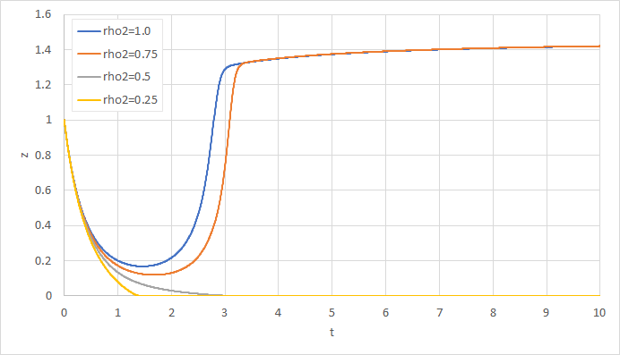
Figure 1. An approximated solution computed on the dense mesh, treated as the reference solution of the model (6.1) with: $\varrho_{2}=1$, $\varrho_{2}=0.75$, $\varrho_{2}=0.5$, and $\varrho_{2}=0.25$.

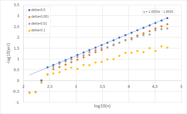
i $-\log_{10}\textrm{(err)}$ vs. $\log_{10}n$ for $\varrho_{2}=1$.

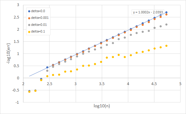
ii $-\log_{10}\textrm{(err)}$ vs. $\log_{10}n$ for $\varrho_{2}=0.75$.

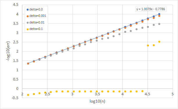
iii $-\log_{10}\textrm{(err)}$ vs. $\log_{10}n$ for $\varrho_{2}=0.5$.

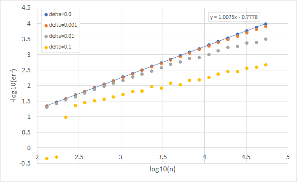
iv $-\log_{10}\textrm{(err)}$ vs. $\log_{10}n$ for $\varrho_{2}=0.25$.

Figure 2. $-\log_{10}\textrm{(err)}$ vs. $\log_{10}n$ for the model (6.1).

In the next experiment we take the following values of the parameters: $a=0$, $b=10$, $A=2$, $B_{1}=-2$, $B_{2}=-0.5$, $\varrho_{1}=1$, $\varrho_{2}=0.75$ but $\alpha=0.4$. In Figure 3 we compare reference solutions for $\alpha\in\{0.4,1.0\}$ with $\delta=0$. In Figure 4 we have test results for $\delta=0$ and $\delta\in\{0.1,0.01,0.001\}$.

From Proposition 5.1 and Fact 7.4 we have the theoretical convergence rate is $O\Bigl{(}h^{\alpha}+h^{\min\{\varrho_{1},\varrho_{2}\}}+\mathbf{1}_{(0,1]}(\delta)\cdot(h^{1/2}+\delta)\Bigr{)}$. As we see in Figure 2 and Figure 4 the bigger $\delta$, the less steep are the empirical convergence rates.

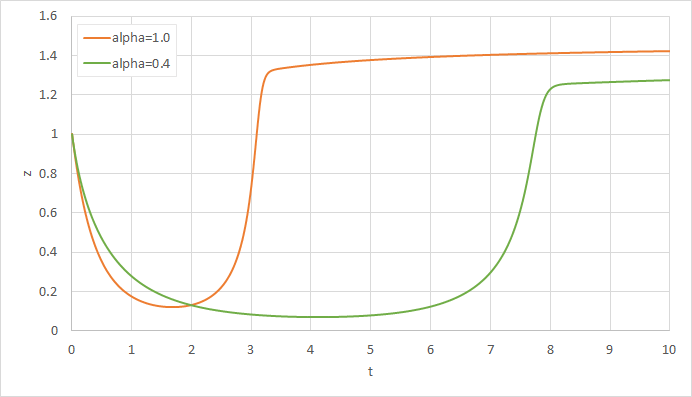
Figure 3. An approximated solution computed on the dense mesh, treated as the reference solution of the model (6.1) with: $\alpha=0.4$, $\alpha=1.0$.

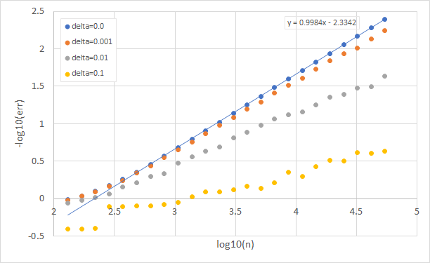
Figure 4. $-\log_{10}\textrm{(err)}$ vs. $\log_{10}n$ for the model (6.1) with $\alpha=0.4$.

6.2. Multiplicative example

Let us consider a family of the following functions

$$g(t,x)=\gamma(t)h(x)f(x),\quad(t,x)\in[a,b]\times\mathbb{R}$$ (6.2)

where $h(x)=-\textrm{sgn}(x)|x|^{\varrho}$, $\varrho\in(0,1]$, and for $\gamma:[a,b]\to\mathbb{R}$, $f:\mathbb{R}\to\mathbb{R}$ the following conditions are satisfied:

• there exists $L_{\gamma}\geq 0$, $\alpha\in(0,1]$ such that for all $t,s\in[a,b]$

  $$|\gamma(t)-\gamma(s)|\leq L_{\gamma}|t-s|^{\alpha},$$ (6.3)

• for all $t\in[a,b]$

  $$\gamma(t)\geq 0,$$ (6.4)

• there exists $D\geq 0$ such that for all $x\in\mathbb{R}$

  $$0\leq f(x)\leq D,$$ (6.5)

• there exists $L_{f}\geq 0$ such that for all $x,y\in\mathbb{R}$

  $$|f(x)-f(y)|\leq L_{f}|x-y|.$$ (6.6)

It turns out that the function (6.2) satisfies the assumptions (G1)-(G4), see Fact 7.5.

For the testing purpose we take the following particular function

$$g(t,x)=-0.3\cdot|\sin(\pi\cdot t+1)|^{2/3}\cdot\textrm{sgn}(x)|x|^{2/3}\cdot|\cos(x)|,$$ (6.7)

with $\varrho=\frac{2}{3}$, $a=-3.5$, $b=3.5$, and with the initial-condition $\xi=3$.

In Figure 5 we show a reference solution for exact information ($\delta=0$). In Figure 6 we present the test results for $\delta=0$ and $\delta\in\{0.1,0.01,0.001\}$.

The reference solution in Figure 5 is a little bit bumpy, therefore we can expect that the bigger noise, the more bumpy is the solution and the more approximation steps must be made to obtain a satisfactory approximated solution, see Figure 6.

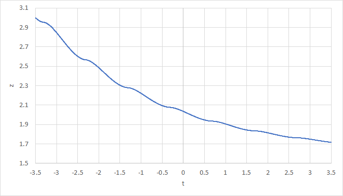
Figure 5. A reference solution of the model (6.2).

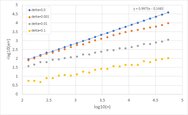
Figure 6. $-\log_{10}\textrm{(err)}$ vs. $\log_{10}n$ for the model (6.2).

Acknowledgments We would like to thank two anonymous reviewers for valuable comments and suggestions that allowed us to improve the quality of the paper.

7. Appendix

In this section we give some auxiliary facts about solution $z$ of the ODE (1.3) and properties of the right-hand side function (6.1). We use the following version of Peano’s theorem.

Theorem 7.1 (Peano’s theorem; [9], page 292., Theorem 70.4).

If the function $g$ satisfies the assumptions (G1) and (G2), then the initial value problem (1.3) has at least one solution that belongs to $C^{1}([a,b]\times\mathbb{R}^{d};\mathbb{R}^{d})$.

Lemma 7.2.

Let $\xi\in\mathbb{R}^{d}$ and let us assume that $g$ satisfies the assumptions (G1), (G2) and (G3). Then there exists a unique solution $z=z(\xi,g)\in C^{1}([a,b];\mathbb{R}^{d})$ of (1.3) and

$$\sup_{a\leq t\leq b}\|z(t)\|\leq K_{0},$$ (7.1)

where $K_{0}=K_{0}(a,b,K,\xi)=(\|\xi\|+K(b-a))e^{K(b-a)}\leq C_{0}(1+\|\xi\|)$ and $C_{0}=C_{0}(a,b,K)=\max\{1,K(b-a)\}e^{K(b-a)}$.

Proof.

By (G1), (G2) and from Theorem 7.1 the equation (1.3) has at least one solution $z=z(\xi,g)\in C^{1}([a,b];\mathbb{R}^{d})$. Hence, by (G2) we get for all $t\in[a,b]$

$$\|z(t)\|\leq\|\xi\|+K(b-a)+K\int\limits_{a}^{t}\|z(s)\|ds,$$ (7.2)

and from the Gronwall’s lemma we obtain that

$$\sup_{a\leq t\leq b}\|z(t)\|\leq K_{0},$$ (7.3)

where $K_{0}=K_{0}(a,b,K,\xi)=(\|\xi\|+K(b-a))e^{K(b-a)}$. Hence, $z(t)\in B_{0}(K_{0})$ for all $t\in[a,b]$.

Let us consider two solutions $z=z(\xi,g)$ and $\tilde{z}=\tilde{z}(\xi,g)$ of (1.3). We have that $z(t),\tilde{z}(t)\in B_{0}(K_{0})$ for all $t\in[a,b]$. By (G3) applied to $U=B_{0}(K_{0})$ we have that there exists $H_{U}\in\mathbb{R}$ such that for all $t\in[a,b]$

$$\frac{d}{dt}\|z(t)-\tilde{z}(t)\|^{2} = \frac{d}{dt}\left\|\int_{a}^{t}(g(s,z(s))-g(s,\tilde{z}(s)))ds\right\|^{2}$$ (7.4)

$$\leq 2\langle z(t)-\tilde{z}(t),g(t,z(t))-g(t,\tilde{z}(t))\rangle$$

$$\leq 2H_{U}\|z(t)-\tilde{z}(t)\|^{2}\leq 2H_{U}^{+}\|z(t)-\tilde{z}(t)\|^{2}.$$

Hence, the $C^{1}$-function $[a,b]\ni t\to\varphi(t)=\|z(t)-\tilde{z}(t)\|^{2}\in[0,+\infty)$, where $\varphi(a)=0$, satisfies the following integral inequality

$$\varphi(t)\leq 2H_{U}^{+}\int_{a}^{t}\varphi(s)ds.$$

From the Gronwall’s lemma we therefore get that $\varphi(t)=0$ for all $t\in[a,b]$, which in turn implies that $z(t)=\tilde{z}(t)$ for all $t\in[a,b]$. ∎

Remark 7.3.

An existence and a uniqueness of the solution of (1.3) assuming (G1)-(G3) follow also from Theorem 3.27. page 182 in [30].

Fact 7.4.

The function (6.1) satisfies the assumptions (G1)-(G4) with $\alpha=\alpha$ and $\beta=\min\{\varrho_{1},\varrho_{2}\}$.

Proof.

We have that $g(t,x)=\sum\limits_{i=1}^{3}h_{i}(t,x)$ where $h_{1}(t,x)=A|t|^{\alpha}x\sin(x^{2}+1)$ and $h_{i}(t,x)=B_{i}\textrm{sgn}(x)|x|^{\varrho_{i}}$ for $i=2,3$, $(t,x)\in[a,b]\times\mathbb{R}$. Of course $h_{i}\in C([a,b]\times\mathbb{R};\mathbb{R})$ for $i=1,2,3$ and therefore $g$ satisfies (G1). Moreover, for all $(t,x)\in[a,b]\times\mathbb{R}$

$$|g(t,x)|\leq|A|D_{1}|x|+(|B_{1}|+|B_{2}|)(1+|x|)\leq\Bigl{(}|A|D_{1}+|B_{1}|+|B_{2}|\Bigr{)}(1+|x|),$$ (7.5)

where $D_{1}=\max\limits_{a\leq t\leq b}|t|^{\alpha}$. Therefore, the function $g$ satisfies (G2). Next, for all $t_{1},t_{2}\in[a,b]$, $x_{1},x_{2}\in\mathbb{R}$ we have that

$$|h_{1}(t_{1},x_{1})-h_{1}(t_{2},x_{2})|\leq|h_{1}(t_{1},x_{1})-h_{1}(t_{1},x_{2})|+|h_{1}(t_{1},x_{2})-h_{1}(t_{2},x_{2})|,$$ (7.6)

where

$$|h_{1}(t_{1},x_{1})-h_{1}(t_{1},x_{2})|\leq\frac{3}{2}|A|\cdot D_{1}\cdot(1+x_{1}^{2}+x_{2}^{2})\cdot|x_{1}-x_{2}|,$$ (7.7)

and, by Lemma A1.3 in [7],

$$|h_{1}(t_{1},x_{2})-h_{1}(t_{2},x_{2})|\leq|A|\cdot|x_{2}|\cdot|t_{1}-t_{2}|^{\alpha}.$$ (7.8)

This implies, in particular, that for all $t\in[a,b]$, $x_{1},x_{2}\in\mathbb{R}$

$$(x_{1}-x_{2})(h_{1}(t,x_{1})-h_{1}(t,x_{2}))\leq|(x_{1}-x_{2})(h_{1}(t,x_{1})-h_{1}(t,x_{2}))|$$

$$=|x_{1}-x_{2}|\cdot|h_{1}(t,x_{1})-h_{1}(t,x_{2})|\leq\frac{3}{2}|A|\cdot D_{1}\cdot(1+x_{1}^{2}+x_{2}^{2})\cdot|x_{1}-x_{2}|^{2}.$$ (7.9)

Since $B_{1},B_{2}\leq 0$, from the proof of Fact A.4 in [7] we have that for all $t\in[a,b]$, $x_{1},x_{2}\in\mathbb{R}$, $i=2,3$

$$(x_{1}-x_{2})(h_{i}(t,x_{1})-h_{i}(t,x_{2}))\leq 0,$$ (7.10)

and for all $t_{1},t_{2}\in[a,b]$, $x_{1},x_{2}\in\mathbb{R}$, $i=2,3$

$$|h_{i}(t_{1},x_{1})-h_{i}(t_{2},x_{2})|\leq 2|B_{i}|\cdot|x_{1}-x_{2}|^{\varrho_{i}}.$$ (7.11)

Hence, by (7), (7.10) we get for all $t\in[a,b]$, $x_{1},x_{2}\in\mathbb{R}$

$$(x_{1}-x_{2})(g(t,x_{1})-g(t,x_{2}))=(x_{1}-x_{2})\cdot\sum\limits_{i=1}^{3}(h_{i}(t,x_{1})-h_{i}(t,x_{2}))$$

$$\leq(x_{1}-x_{2})(h_{1}(t,x_{1})-h_{1}(t,x_{2}))\leq\frac{3}{2}|A|\cdot D_{1}\cdot(1+x_{1}^{2}+x_{2}^{2})\cdot|x_{1}-x_{2}|^{2}.$$ (7.12)

Since for every $U\in\textrm{comp}(\mathbb{R})$ there exists a ball $B_{0}(R)$, with the radius $R\in(0,+\infty)$, such that $U\subset B_{0}(R)$, for all $t\in[a,b]$, $x_{1},x_{2}\in U$ we have

$$(x_{1}-x_{2})(g(t,x_{1})-g(t,x_{2}))\leq\frac{3}{2}|A|\cdot D_{1}\cdot(1+2R^{2})\cdot|x_{1}-x_{2}|^{2},$$ (7.13)

and, by (7.7),(7.8), (7.11), for all $t_{1},t_{2}\in[a,b]$, $x_{1},x_{2}\in\mathbb{R}$

$$|g(t_{1},x_{1})-g(t_{2},x_{2})|\leq\sum\limits_{i=1}^{3}|h_{i}(t_{1},x_{1})-h_{i}(t_{2},x_{2})|$$

$$\leq|A|\cdot R\cdot|t_{1}-t_{2}|^{\alpha}+\max\Bigl{\{}\frac{3}{2}|A|D_{1}(1+2R^{2}),2|B_{1}|,2|B_{2}|\Bigr{\}}\cdot 3(1+2R)\cdot|x_{1}-x_{2}|^{\min\{\varrho_{1},\varrho_{2}\}}.$$

Hence, $g$ satisfies also (G3), (G4), and this ends the proof. ∎

Fact 7.5.

The function (6.2) satisfies the assumptions (G1)-(G4) with $\alpha=\alpha$ and $\beta=\varrho$.

Proof.

Of course, $g\in C([a,b]\times\mathbb{R};\mathbb{R})$ and therefore $g$ satisfies (G1). Furthermore, for all $(t,x)\in[a,b]\times\mathbb{R}$

$$|g(t,x)| \leq D\sup_{t\in[a,b]}|\gamma(t)|(1+|x|),$$

hence $g$ satisfies (G2) with $K=D\sup\limits_{t\in[a,b]}|\gamma(t)|$. Moreover, $h$ is monotonically decreasing, thus for all $t\in[a,b]$ and $x,y\in\mathbb{R}$

$$(x-y)\Bigl{(}g(t,x)-g(t,y)\Bigr{)} =\gamma(t)(x-y)\Bigl{(}h(x)f(x)-h(y)f(y)\Bigr{)}$$

$$=\gamma(t)f(x)(x-y)(h(x)-h(y))+\gamma(t)(x-y)h(y)(f(x)-f(y))$$

$$\leq\gamma(t)(x-y)h(y)(f(x)-f(y))\leq|\gamma(t)(x-y)h(y)(f(x)-f(y))|$$

$$\leq L_{f}\sup_{t\in[a,b]}|\gamma(t)|\cdot(1+|y|)\cdot|x-y|^{2}.$$

For all $U\in\textrm{comp}(\mathbb{R})$ there exists a ball $B_{0}(R)$, $R>0$, such that $U\subset B_{0}(R)$ and for all $t\in[a,b]$, $x,y\in U$ we have

$$(x-y)\Bigl{(}g(t,x)-g(t,y)\Bigr{)}\leq L_{f}\sup_{t\in[a,b]}|\gamma(t)|\cdot(1+R)\cdot|x-y|^{2}.$$

Hence, $g$ satisfies the assumption (G3). Furthermore, for all $t_{1},t_{2}\in[a,b]$ and $y_{1},y_{2}\in\mathbb{R}$ we have

$$|g(t_{1},y_{1})-g(t_{2},y_{2})|\leq|g(t_{1},y_{1})-g(t_{2},y_{1})|+|g(t_{2},y_{1})-g(t_{2},y_{2})|,$$

where

$$|g(t_{1},y_{1})-g(t_{2},y_{1})|\leq L_{\gamma}D\cdot(1+|y_{1}|)\cdot|t_{1}-t_{2}|^{\alpha},$$ (7.14)

and

$$|g(t_{2},y_{1})-g(t_{2},y_{2})| \leq L_{f}\sup_{t\in[a,b]}|\gamma(t)|\cdot(1+|y_{1}|)\cdot|y_{1}-y_{2}|+2D\sup_{t\in[a,b]}|\gamma(t)|\cdot|y_{1}-y_{2}|^{\varrho}$$

$$\leq\sup_{t\in[a,b]}|\gamma(t)|\cdot\max\{L_{f},D\}\cdot\Bigl{[}(1+|y_{1}|)\cdot(1+|y_{1}|+|y_{2}|)+2\Bigr{]}\cdot|y_{1}-y_{2}|^{\varrho}.$$

Thus, since for all $U\in\textrm{comp}(\mathbb{R})$ there exists a ball $B_{0}(R)$, $R>0$, such that $U\subset B_{0}(R)$, for all $t_{1},t_{2}\in[a,b]$, $y_{1},y_{2}\in U$ we have

$$|g(t_{1},y_{1}) - g(t_{2},y_{2})|\leq L_{\gamma}D(1+R)|t_{1}-t_{2}|^{\alpha}$$

$$+\sup_{t\in[a,b]}|\gamma(t)|\cdot\max\{L_{f},D\}\Bigl{[}(1+R)(1+2R)+2\Bigr{]}|y_{1}-y_{2}|^{\varrho}.$$

This implies that $g$ satisfies (G4) with $\alpha=\alpha$ and $\beta=\varrho$, and the proof is completed. ∎

References

• [1] W. F. Ames, Numerical methods for partial differential equations. 3rd ed., Academic Press, San Diego, 1992.
• [2] T. Bochacik, P. Przybyłowicz, On the randomized Euler schemes for ODEs under inexact information, Numer. Algor., 91(3) (2022), 1205–1229.
• [3] T. Bochacik, M. Goćwin, P. M. Morkisz, P. Przybyłowicz, Randomized Runge–Kutta method—Stability and convergence under inexact information, J. Complexity 65 (2021), 101554.
• [4] J. C. Butcher, Numerical methods for ordinary differential equations. 3rd ed., Wiley, Chichester, 2016.
• [5] E. W. Cheney, D. R. Kincaid, Numerical Mathematics and Computing, 7th ed., Brooks/Cole Cengage Learning, Boston, 2012.
• [6] N. Czyżewska, J. Kusiak, P. Morkisz, P. Oprocha, M. Pietrzyk, P. Przybyłowicz, Ł. Rauch, D. Szeliga, On mathematical aspects of evolution of dislocation density in metallic materials, IEEE Access 10 (2022), 86793–86812.
• [7] N. Czyżewska, P. M. Morkisz, P. Przybyłowicz, Approximation of solutions of DDEs under nonstandard assumptions via Euler scheme, Numer. Algor., 91(3) (2022), 1829–1854.
• [8] R. D. Driver, Ordinary and delay differential equations. Springer-Verlag, New York, 1977.
• [9] L. Górniewicz, R. S. Ingarden, Mathematical Analysis for Physicists (in Polish). Wydawnictwo Naukowe UMK, 2012.
• [10] Griffiths D. F., Higham D. J., Numerical Methods for Ordinary Differential Equations. Initial Value Problems. Springer-Verlag, London, 2010.
• [11] E. Hairer and G. Wanner, Solving Ordinary Differential Equations II. Stiff and Differential-Algebraic Problems, 2nd rev. ed., Springer-Verlag, Heidelberg, New York, 2010.
• [12] S. Heinrich, Complexity of initial value problems in Banach spaces, Zh. Mat. Fiz. Anal. Geom. 9 (2013), 73–101.
• [13] Z. Jackiewicz, General linear methods for ordinary differential equations. Wiley, Hoboken, New Jersey, 2009.
• [14] B. Kacewicz, Optimal solution of ordinary differential equations, J. Complex. 3 (1987), 451–465.
• [15] B. Kacewicz, M. Milanese, A. Vicino, Conditionally optimal algorithms and estimation of reduced order models, J. Complex. 4 (1988), 73–85.
• [16] B. Kacewicz, L. Plaskota, On the minimal cost of approximating linear problems based on information with deterministic noise, Numer. Funct. Anal. and Optimiz. 11 (1990), 511-528.
• [17] B. Kacewicz, P. Przybyłowicz, On the optimal robust solution of IVPs with noisy information, Numer. Algor. 71 (2016), 505–518.
• [18] B. Kacewicz, P. Przybyłowicz, Efficient finite-dimensional solution of initial value problems in infinite-dimensional Banach spaces, J. Math. Anal. Appl. 471 (2019), 322-341.
• [19] A. Kałuża, P. M. Morkisz, P. Przybyłowicz, Optimal approximation of stochastic integrals in analytic noise model, Appl. Math. and Comput. 356 (2019), 74–91.
• [20] P. E. Kloeden, E. Platen, Numerical Solution of Stochastic Differential Equations. Springer-Verlag, Berlin, 3rd ed., 1999.
• [21] S. Larsson, V. Thomée, Partial differential equations with numerical methods. Springer-Verlag, Berlin, 2003.
• [22] S. Mazumder, Numerical methods for partial differential equations. Finite difference and finite volume methods. Academmic Press, London, 2016.
• [23] M. Milanese, A. Vicino, Optimal estimation theory for dynamic systems with set membership uncertainty: an overview, Automatica 27 (1991), 997–1009.
• [24] G. N. Milstein, M. V. Tretyakov, Stochastic Numerics for Mathematical Physics. Springer-Verlag, Berlin, 2004.
• [25] P. M. Morkisz, L. Plaskota, Approximation of piecewise Hölder functions from inexact information, J. Complex. 32 (2016), 122–136.
• [26] P. M. Morkisz, L. Plaskota, Complexity of approximating Hölder classes from information with varying Gaussian noise, to appear in J. Complex. 60 (2020), ID 101497.
• [27] P. M. Morkisz, P. Przybyłowicz, Optimal pointwise approximation of SDE’s from inexact information, J. Comput. Appl. Math. 324 (2017), 85–100.
• [28] P. M. Morkisz, P. Przybyłowicz, Randomized derivative-free Milstein algorithm for efficient approximation of solutions of SDEs under noisy information, J. Comput. Appl. Math. 383 (2021), ID 113112.
• [29] E. Novak, Deterministic and Stochastic Error Bounds in Numerical Analysis, Lecture Notes in Mathematics, vol. 1349, New York, Springer–Verlag, 1988.
• [30] E. Pardoux, A. Rascanu, Stochastic Differential Equations, Backward SDEs, Partial Differential Equations, Stochastic Modelling and Applied Probability, Springer International Publishing Switzerland, 2014.
• [31] L. Plaskota, Noisy Information and Computational Complexity, Cambridge Univ. Press, Cambridge, 1996.
• [32] L. Plaskota, Noisy information: optimality, complexity, tractability, in Monte Carlo and quasi-Monte Carlo Methods 2012, J. Dick, F.Y. Kuo, G.W. Peters, I.H. Sloan (Eds.), Springer 2013, 173–209.
• [33] A.A. Samarskii, The Theory of Difference Schemes. Marcel Dekker, New York, 2001.
• [34] J.F. Traub, G.W. Wasilkowski, H. Woźniakowski, Information-Based Complexity, Academic Press, New York, 1988.
• [35] A.G. Werschulz, The complexity of definite elliptic problems with noisy data. J. Complex. 12 (1996), 440-473.
• [36] A.G. Werschulz, The complexity of indefinite elliptic problems with noisy data. J. Complex. 13 (1997), 457-479.