Neural Networks Reduction via Lumping

Abstract

The increasing size of recently proposed Neural Networks makes it hard to implement them on embedded devices, where memory, battery and computational power are a non-trivial bottleneck. For this reason during the last years network compression literature has been thriving and a large number of solutions has been been published to reduce both the number of operations and the parameters involved with the models. Unfortunately, most of these reducing techniques are actually heuristic methods and usually require at least one re-training step to recover the accuracy.

The need of procedures for model reduction is well-known also in the fields of Verification and Performances Evaluation, where large efforts have been devoted to the definition of quotients that preserve the observable underlying behaviour.

In this paper we try to bridge the gap between the most popular and very effective network reduction strategies and formal notions, such as lumpability, introduced for verification and evaluation of Markov Chains. Elaborating on lumpability we propose a pruning approach that reduces the number of neurons in a network without using any data or fine-tuning, while completely preserving the exact behaviour. Relaxing the constraints on the exact definition of the quotienting method we can give a formal explanation of some of the most common reduction techniques.

1 Introduction

Since 2012, when AlexNet [26] won the famous ImageNet Large Scale Visual Recognition Challenge (ILSVRC), the number of proposed Artificial Neural Network (ANN or NN) architectures has increased exponentially. Their intrinsic flexibility, together with the superior performance they can achieve, made neural networks the tool of choice to solve a wide variety of tasks. As these models have evolved to process large amount of data or to solve complicated tasks, their complexity has also increased at same pace [10]. Such elaborate and deep networks are the foundation of Deep Learning (DL) and they stand out both for the large number of layers they are made of and for the higher level of accuracy they can reach on difficult tasks [53].

While the academic community mostly focused their efforts in training large and deep models [25, 8, 54], being able to adopt such networks in embedded devices resulted to be a problem. Physical constraints such as battery, memory and computational power greatly limit both the number of parameters used to the define the architecture and the number of Floating Point Operations (FLOPs) required to be computed at inference time. A commonly used strategy to address this problem is called Network Compression. Compression literature has had a substantial growth during the last years, and for this reason there are many different ways to group together methods reducing a model in similar ways.

Methods focusing on finding the best possible structure to solve a particular tasks can be grouped together as Architecture-related strategies. These kind of methods usually require to train the network from scratch each time the structure is modified. In particular, Neural Architecture Search (NAS) techniques aim to find the best possible architecture for a certain task with minimal human intervention [41, 12, 32]. This is usually made possible by modelling the search as an optimization problem and applying Reinforcement Learning (LR)-based methods to find the best architecture [57, 3]. In this group we can also find Tensor Decomposition, where matrix decomposition/factorization principles are applied to the $d$-dimensional tensors in neural networks. Tensor decomposition generalizes the widely used Principal Component Analysis (PCA) and Singular Value Decomposition (SVD) to an arbitrary number of dimensions [6, 16, 51]. The goal of these techniques is to reduce the rank of tensors in order to efficiently decompose them into smaller ones and drastically reduce the number of operations [10]. As the rank of a tensor is usually far from being small, the most common solutions are to either to force the network to learn filters with small rank either to use an approximated decomposition [11].

Using a similar approach Lightweight or Compact Networks focus on modifying the design of the architecture such that it performs less operations while maintaining the same capability. It is the case of the MobileNet series [21, 43, 20], ShuffleNet series [56, 34], and EfficientNet series [49, 50]. They exploit the idea of using 1$\times$1 filters introduced by Network in Network [29] and GoogLeNet [46, 47] in their inception modules. A similar concept is explored by the SqueezeNet [23] architecture in their Fire module, where they substitute the classical convolutional layers such that they can achieve the same accuracy of AlexNet on ImageNet dataset but with a model 510 times smaller.

A different methodology consists in training a big model from the start, and then Pruning superfluous parameters. In particular, Weight Pruning consists in zeroing connections or parameters already close to zero [27], but more elaborated methods can also take into consideration the impact of the single weights on the final results [15]. Even if weight pruning is a very powerful tool to reduce the network parameters [13], its major drawback is that it does not actually reduce the number of FLOPs at inference time.

A more effective solution consists instead in skipping completely some of the operations. It is the case of Filter Pruning, where whole nodes or filters (in case of convolutional layers) are removed from the architecture. Pruning usually requires some degree of re-training to recover the lost accuracy due to the reduced network capability, but an interesting phenomena that happens in the early stages of pruning is that most of the times the test accuracy actually increases, due to the regularization effect that pruning unnecessary parameters has on the network. While weight pruning allows more control on what parameters to remove, filter pruning is usually the best solution compression-wise as it allows to drastically reduce the network parameters such that the models can be actually implemented in small embedded devices [42].

Another technique often used in conjunction with pruning is called quantization [14]. While pruning aims to reduce the number of parameters, quantization instead targets their precision. As the weights are usually represented by floating point numbers, it is possible to reduce the bits used for the number representation down to single bits [40], without affecting the network accuracy.

In the context of performance evaluation of computer systems, stochastic models whose underlying stochastic processes are Markov chains, play a key role providing a sound high-level framework for the analysis of software and hardware architectures. Although the use of high-level modelling formalism greatly simplifies the specification of quantitative models (e.g., by exploiting the compositionality properties [18]), the stochastic process underlying even a very compact model may have a number of states that makes its analysis a difficult, sometimes computationally impossible, task. In order to study models with a large state space without using approximations or resorting to simulations, one can attempt to reduce the state space of the underlying Markov chain by aggregating states with equivalent behaviours. Lumpability is an aggregation technique used to cope with the state space explosion problem inherent to the computation of the stationary performance indices of large stochastic models. The lumpability method turns out to be useful on Markov chains exhibiting some structural regularity. Moreover, it allows one to efficiently compute the exact values of the performance indices when the model is actually lumpable. In the literature, several notions of lumping have been introduced: ordinary and weak lumping [24], exact lumping [44], and strict lumping [5].

With this paper we aim to link together the work of two different communities, the first one focusing on machine learning and network compression and the second one focusing on lumping-based aggregation techniques for performance evaluation. Even if a large number of possible efficient compression techniques has already been published, we aim instead to give a formal demonstration on how it is possible to deterministically remove some of the network parameters to obtain a smaller network with the same performance. Our method condenses many different concepts together, such as some of the ideas exploited by tensor decomposition methods, filter pruning and the lumpability used to evaluate the performance of complex systems.

The paper is structured as follows. In Section 2 we provide a literature review. Section 3 gives the necessary background. Section 4 formally describes our technique exploiting exact lumpability for quotienting NN. Section 5 presents some experimental results. Finally, Section 6 concludes the paper.

2 Related Work

To the best of our knowledge, the only paper similar to our work is [39], where the authors introduce the classical notion of equivalence between systems in Process Algebra to reduce a neural network into another one semantically equivalent. They propose a filter pruning technique based on some properties of the network that does not need any data to perform the compression. They also define an approximated version of their algorithm to relax some of the strong constraints they pose on the weights of the network.

While data free pruning algorithms are convenient when a dataset is incomplete, unbalanced or missing, they usually achieve poorer results compared to data-based compression solutions. Indeed, most pruning techniques usually require at least one stage of fine-tuning of the model. The recovery is often performed in an iterative fashion after removing a single parameter, but there are also techniques that re-train the model only after a certain level of compression has been carried out [4].

As defined in [30] filter pruning techniques can be divided according to property importance or adaptive importance. In the first group we find pruning methods that look at intrinsic properties of the networks, and do not modify the training loss, such as [39, 22, 28, 17, 42, 7]. Adaptive importance pruning algorithms like [33, 31] usually drastically change the loss function, requiring a heavy retrain step and to look for a new proper set of hyper-parameters, despite the fact that they often achieve better performances with respect to property importance methods. Avoiding to re-train the network at each pruning step as in [30, 52] is usually faster than other solutions, but there is a higher risk to not being able to recover the performances.

Another option consists in deciding which parameters to remove according to the impact they have on the rest of the network [37, 55]. Finally, while most of the already mentioned methods focus on removing whole filters or kernels from convolutional layers, some other methods actually target only fully connected layers, or are made to compress classical neural networks [48, 2].

3 Preliminaries

In this section we formally introduce the notion of neural network in the style of [39]. Moreover, we recall the concept of exact lumpabibility as it has been defined in the context of continuous time Markov chains.

Neural Networks

A neural network is formed by a layered set of nodes or neurons, consisting of an input layer, an output layer and one or more hidden layers. Each node that does not belong to the input layer is annotated with a bias and an activation function. Moreover, there are weighted edges between nodes of adjacent layers. We use the following formal definition of neural network.

For $k\in\mathbb{N}$, we denote by $[k]$ the set $\{0,1,\ldots,k\}$, by $(k]$ the set $\{1,\ldots,k\}$, by $[k)$ the set $\{0,\ldots,k-1\}$, and by $(k)$ the set $\{1,\ldots,k-1\}$.

Definition 1 (Neural Network)

A Neural Network (NN) is a tuple $\mathcal{N}=(k,\mathcal{A}ct,\{\mathcal{S}_{\ell}\}_{\ell\in[k]},\{W_{\ell}\}_{\ell\in(k]},\{b_{\ell}\}_{\ell\in(k]},\{A_{\ell}\}_{\ell\in(k]})$ where:

• $k$ is the number of layers (except the input layer);

• $\mathcal{A}ct$ is the set of activation functions;

• for $\ell\in[k]$, $\mathcal{S}_{\ell}$ is the set of nodes of layer $\ell$ with $\mathcal{S}_{\ell}\cap\mathcal{S}_{\ell^{\prime}}=\emptyset$ for $\ell\neq\ell^{\prime}$;

• for $\ell\in(k]$, $W_{\ell}:\mathcal{S}_{\ell-1}\times\mathcal{S}_{\ell}\rightarrow\mathbb{R}$ is the weight function that associates a weight with edges between nodes at layer $\ell-1$ and $\ell$;

• for $\ell\in(k]$, $b_{\ell}:\mathcal{S}_{\ell}\rightarrow\mathbb{R}$ is the bias function that associates a bias with nodes at layer $\ell$;

• for $\ell\in(k]$, $A_{\ell}:\mathcal{S}_{\ell}\rightarrow\mathcal{A}ct$ is the activation association function that associates an activation function with nodes of layer $\ell$.

$\mathcal{S}_{0}$ and $\mathcal{S}_{k}$ denote the nodes in the input and output layers, respectively.

In the rest of the paper we will refer to NNs in which all the activation association function are constant, i.e., all the neurons of a layer share the same activation function. Moreover, such activation functions are either ReLU (Rectified Linear Unit) or LeakyReLU, i.e., they are combinations of linear functions. So, from now on we omit the set $\mathcal{A}ct$ from the definition of the NNs.

Figure 1: Node $v$ behaviour on input $x_{1},x_{2},\dots,x_{m}$

Example 1

Figure 1 shows the behaviour of node $v$ in Layer $\ell$. The input values $x_{1},x_{2},\dots x_{m}$ are propagated by nodes $u_{1},u_{2},\dots u_{m}$ respectively. Node $v$ computes the $ReLU$ of the weighted sum of the inputs plus the bias. The result of this application is the output of $v$ and it is propagated to $z$.

The operational semantics of a neural network is as follows. Let $v:\mathcal{S}_{\ell}\rightarrow\mathbb{R}$ be a valuation for the $\ell$-th layer of $\mathcal{N}$ and $Val(\mathcal{S}_{\ell})$ be the set of all valuations for the $\ell$-th layer of $\mathcal{N}$. The operational semantics of $\mathcal{N}$, denoted by $[\![\mathcal{N}]\!]$, is defined in terms of the semantics of its layers $[\![\mathcal{N}]\!]_{\ell}$, where each $[\![\mathcal{N}]\!]_{\ell}$ associates with any valuation $v$ for layer $\ell-1$ the corresponding valuation for layer $\ell$ according to the definition of $\mathcal{N}$. The valuation for the output layer of $\mathcal{N}$ is then obtained by the composition of functions $[\![\mathcal{N}]\!]_{\ell}$.

Definition 2

The semantics of the $\ell$-th layer is the function $[\![\mathcal{N}]\!]_{\ell}:Val(\mathcal{S}_{\ell-1})\rightarrow Val(\mathcal{S}_{\ell})$ where for all $v\in Val(\mathcal{S}_{\ell-1})$, $[\![\mathcal{N}]\!]_{\ell}(v)=v^{\prime}$ and for all $s^{\prime}\in\mathcal{S}_{\ell}$,

$$v^{\prime}(s^{\prime})=A_{\ell}(s^{\prime})\big{(}\sum_{s\in\mathcal{S}_{\ell-1}}W_{\ell}(s,s^{\prime})v(s)+b_{\ell}(s^{\prime})\big{)}\,.$$

The input-output semantics of $\mathcal{N}$ is obtained by composing these one layer semantics. More precisely, we denote by $[\![\mathcal{N}]\!]^{\ell}$ the composition of the first $\ell$ layers so that $[\![\mathcal{N}]\!]^{\ell}(v)$ provides the valuation of the $\ell$-th layer given $v\in Val(\mathcal{S}_{0})$ as input. Formally, $[\![\mathcal{N}]\!]^{\ell}$ is inductively defined by:

$$[\![\mathcal{N}]\!]^{1}=[\![\mathcal{N}]\!]_{1}$$

$$[\![\mathcal{N}]\!]^{\ell}=[\![\mathcal{N}]\!]_{\ell}\circ[\![\mathcal{N}]\!]^{\ell-1}\ \forall\ell\in(k]$$

where $\circ$ denotes the function composition.

We are now in position to define the semantics of $\mathcal{N}$ as the input-output semantic function $[\![\mathcal{N}]\!]$ defined below.

Definition 3

The input-output semantic function $[\![\mathcal{N}]\!]:Val(\mathcal{S}_{0})\rightarrow Val(\mathcal{S}_{k})$ is defined as

$$[\![\mathcal{N}]\!]=[\![\mathcal{N}]\!]^{k}\,.$$

Lumpability

The notion of lumpability has been introduced in the context of performance and reliability analysis. It provides a model aggregation technique that can be used for generating a Markov chain that is smaller than the original one while allowing one to determine exact results for the original process.

The concept of lumpability can be formalized in terms of equivalence relations over the state space of the Markov chain. Any such equivalence induces a partition on the state space of the Markov chain and aggregation is achieved by clustering equivalent states into macro-states, reducing the overall state space.

Let $\mathcal{S}$ be a finite state space. A (time-homogeneous) Continuous-Time Markov Chain (CTMC) over $\mathcal{S}$ is defined by a function

$$Q:\mathcal{S}\times\mathcal{S}\rightarrow\mathbb{R}$$

such that for all $u,v\in\mathcal{S}$ with $u\neq v$ it holds that:

• $Q(u,v)\geq 0$ and

• $\sum_{v\in\mathcal{S},v\neq u}Q(u,v)=-Q(u,u)\,.$

A CTMC defined over $\mathcal{S}$ by $Q$ models a stochastic process where a transition from $u$ to $v$ can occur according to an exponential distribution with rate $Q(u,v)$.

Given an initial probability distribution $p$ over the states of a CTMC, one can consider the problem of computing the probability distribution to which $p$ converges when the time tends to infinity. This is the stationary distribution and it exists only when the chain satisfies additional constraints. The stationary distribution reveals the limit behaviour of a CTMC. Many other performance indexes and temporal logic properties can be defined for studying both the transient and limit behaviour of the chain.

Different notions of lumpability have been introduced with the aim of reducing the number of states of the chain, while preserving its behaviour [1, 5, 19, 24, 35, 36, 44]. In particular, we consider here the notion of exact lumpability [5, 44].

Definition 4 (Exact Lumpability)

Let $(\mathcal{S},Q)$ be a CTMC and $\mathcal{R}$ be an equivalence relation over $\mathcal{S}$. $\mathcal{R}$ is an exact lumpability if for all $S,S^{\prime}\in\mathcal{R}/\mathcal{S}$, for all $v,t\in S$ it holds that:

$$\sum_{u\in S^{\prime}}Q(u,v)=\sum_{u\in S^{\prime}}Q(u,t)\,.$$

There exists always a unique maximum exact lumpability relation which allows to quotient the chain by taking one state for each equivalence class and replacing the rates of the incoming edges with the sum of the rates from equivalent states.

The notion of exact lumpability is in many applicative domains too demanding, thus providing poor reductions. This issue is well-known for all lumpability notions that do not allow any form of approximation. With the aim of obtaining smaller quotients, still avoiding rough approximations, the notion of proportional lumpability has been presented in [35, 36, 38] as a relaxation of ordinary lumpability. In this paper instead we introduce to proportional exact lumpability which is defined as follows.

Definition 5 (Proportional Exact Lumpability)

Let $(\mathcal{S},Q)$ be a CTMC and $\mathcal{R}$ be an equivalence relation over $\mathcal{S}$. $\mathcal{R}$ is a proportional exact lumpability if there exists a function $\rho:\mathcal{S}\rightarrow\mathbb{R}_{>0}$ such that for all $S,S^{\prime}\in\mathcal{R}/\mathcal{S}$, for all $v,t\in S$ it holds that:

$$\rho(v)\sum_{u\in S^{\prime}}Q(u,v)=\rho(t)\sum_{u\in S^{\prime}}Q(u,t)\,.$$

It can be proved that there exists a unique maximum proportional exact lumpability which can be computed in polynomial time. This is true also if $(\mathcal{S},Q)$ is a Labelled Graph instead of a CTMC, i.e., no constraints are imposed on $Q$.

Figure 2: Proportionally exact lumpable CTMC.

Example 2

Figure 2 shows a proportionally exact lumpable Markov chain with respect to the function $\rho$ defined as: $\rho(1)=1,\rho(2)=1,\rho(3)=2,\rho(4)=1,\rho(5)=1,\rho(6)=2,\rho(7)=1,\rho(8)=1$ and the equivalence classes $S_{1}=\{1\},S_{2}=\{2,3,4\},S_{3}=\{5,6,7\},S_{4}=\{8\}$.

4 Lumping Neural Networks

The idea of exploiting exact lumpability for quotienting NN has been proposed in [39] where a notion of pre-sum preserving backward bisimulation has been considered. It can be easily observed that such a notion coincides with that of exact lumpability. The term (probabilistic) bisimulation is standard in the area of Model Checking, where (probabilistic) temporal logical properties are used for both specifying and synthesizing systems having a desired behaviour (see, e.g., [9]). Since such logics usually formalize the behaviours in terms of forward temporal operators, the bisimulation notions tend to preserve the rates of the outgoing edges [45]. However, as proved in [39], in order to preserve the behaviour of a NN it is necessary to refer to the rates/weights of the incoming edges. This is referred to as backward probabilistic bisimulation and coincides with the well-known notion of exact lumpability used in the area of performances evaluation.

In this paper we extend the proposal of [39]. We prove that in the case of ReLU and LeakyReLU activations, proportional exact lumpability preserves the behaviour of the network allowing to obtain smaller quotients. It does not require any retraining step and it ensures the same behaviour on all possible inputs. Moreover, since the neural networks we refer to are acyclic it can be computed in linear time.

Definition 6 (Proportional Exact Lumpability over a NN)

Let $\mathcal{N}$ be a NN. Let $\mathcal{R}=\cup_{\ell\in[k)}\mathcal{R}_{\ell}$ be such that $\mathcal{R}_{\ell}$ is an equivalence relation over $\mathcal{S}_{\ell}$, for all $\ell\in(k)$ and $\mathcal{R}_{0}$ is the identity relation over $\mathcal{S}_{0}$. We say that $\mathcal{R}$ is a proportional exact lumpability over $\mathcal{N}$ if for each $\ell\in(k)$ there exists $\rho_{\ell}:\mathcal{S}_{\ell}\rightarrow\mathcal{R}_{>0}$ such that for all $S\in\mathcal{S}_{\ell}$, for all $S^{\prime}\in\mathcal{S}_{\ell-1}$, for all $v,t\in S$ it holds that:

$$\begin{array}[]{c}\rho_{\ell}(v)b_{\ell}(v)=\rho_{\ell}(t)b_{\ell}(t)\,,\\[5.69046pt] \rho_{\ell}(v)\sum_{u\in S^{\prime}}W_{\ell}(u,v)=\rho_{\ell}(t)\sum_{u\in S^{\prime}}W_{\ell}(u,t)\,.\end{array}$$

There are some differences with respect to the definition of proportional exact lumpability over CTMCs. First, we impose that two equivalent neurons have to belong to the same layer. However, we could have omitted such restriction from the definition and proved that neurons from different layers are never equivalent. This is an immediate consequence of the fact that we refer to acyclic NNs. Moreover, we demand that on input and output nodes the only admissible relation is the identity. This is a substantial difference. Since the nodes in the input layer have no incoming edges the definition of proportional lumpability given over CTMCs allows to collapse them. However, the input nodes in NNs hold the input values that have to be propagated, so they cannot be collapsed. This is true also for the output nodes, since they represent the result of the computation.

It can be proved that there always exists a unique maximum proportional exact lumpability over a NN. If we use proportional exact lumpability for reducing the dimension of a NN by collapsing the equivalent neurons, we have to modify the topology and the weights of the NN as formalized below.

Definition 7 (Proportional Reduced NN)

Let $\mathcal{N}=(k,\{\mathcal{S}_{\ell}\}_{\ell\in[k]},$ $\{W_{\ell}\}_{\ell\in(k]},$ $\{b_{\ell}\}_{\ell\in(k]},\{A_{\ell}\}_{\ell\in(k]})$ be a NN. Let $\mathcal{R}$ be a proportional exact lumpability over $\mathcal{N}$. The NN $\mathcal{N}/\mathcal{R}=(k,\{\mathcal{S}^{\prime}_{\ell}\}_{\ell\in[k]},\{W^{\prime}_{\ell}\}_{\ell\in(k]},\{b^{\prime}_{\ell}\}_{\ell\in(k]},\{A^{\prime}_{\ell}\}_{\ell\in(k]})$ is defined by:

• $\mathcal{S}^{\prime}_{\ell}=\{[v]\>|\>[v]\in\mathcal{S}_{\ell}/\mathcal{R}\}$, where $v$ is an arbitrarily chosen representative for the class;

• $W_{\ell}^{\prime}([u],[v])=\rho_{\ell-1}(u)\sum_{w\in[u]}\frac{W_{\ell}(w,v)}{\rho_{\ell-1}(w)}$;

• $b_{\ell}^{\prime}([v])=b_{\ell}(v)$;

• $A^{\prime}_{\ell}([v])=A_{\ell}(v)$.

Despite the arbitrary choice of the representative, we can prove that the reduced NN’s behaviour coincides with that of the initial one over all the inputs.

Theorem 4.1

Let $\mathcal{N}$ be a NN and $\mathcal{R}$ be a proportional exact lumpability over $\mathcal{N}$. It holds that

$$[\![\mathcal{N}/\mathcal{R}]\!]=[\![\mathcal{N}]\!]\,.$$

Proof

Sketch. Let us focus on two neurons $v$ and $t$ belonging to layer $1$ that are equivalent in $\mathcal{R}_{1}$. Let $ReLU$ be the activation function for both of them.

On input $x_{1},x_{2},\dots x_{m}$ for the nodes $u_{1},u_{2},\dots,u_{m}$ of layer $0$ the nodes $v$ and $t$ take values $Val(v)=ReLU(\sum_{j=1}^{m}W_{1}(u_{j},v)x_{j}+b_{1}(v))$ and $Val(t)=ReLU(\sum_{j=1}^{m}W_{1}(u_{j},t)x_{j}+b_{1}(t))$, respectively. However, since $v$ and $t$ are equivalent, it holds that:

$$\sum_{j=1}^{m}W_{1}(u_{j},t)x_{j}+b_{1}(t)=\frac{\rho_{1}(v)}{\rho_{1}(t)}\sum_{j=1}^{m}W_{1}(u_{j},v)x_{j}+b_{1}(v)$$

Since $\rho_{1}(v)$ and $\rho_{1}(t)$ are positive numbers, we get that:

$$\begin{array}[]{lcl}Val(t)&=&ReLU(\sum_{j=1}^{m}W_{1}(u_{j},t)x_{j}+b_{1}(t))\\ &=&\frac{\rho_{1}(v)}{\rho_{1}(t)}ReLU(\sum_{j=1}^{m}W_{1}(u_{j},v)x_{j}+b_{1}(v))=\frac{\rho_{1}(v)}{\rho_{1}(t)}Val(v)\,.\end{array}$$

Let now $z$ be a neuron of layer $2$. The value of $z$ depends on

$$W_{2}(v,z)Val(v)+W_{2}(t,z)Val(t)=(W_{2}(v,z)+\frac{\rho_{1}(v)}{\rho_{1}(t)}W_{2}(t,z))Val(v)$$

So, the definition of $W_{2}^{\prime}$ takes care of the fact that in the reduced network $v$ represents the equivalence class, while $t$ has been “eliminated”. Such definition ensures that the value of neuron $z$ is unchanged.

A formal proof can be obtained generalizing the above arguments. ∎

Figure 3: Pruning one node and updating the network.

Example 3

Figure 3 shows how the pruning technique works on two nodes $v,t$. In particular, $t$ input weights are proportionals to $v$’s. The algorithm proceeds in two steps. Firstly, $t$ is deleted together with all its input and output edges. Secondly, the weight from $v$ to $z$ is modified by adding $W_{\ell+1}(t,z)/\rho$.

The maximum proportional exact lumpability over $\mathcal{N}$ together with the reduced network can be efficiently computed by proceeding top-down from layer $1$ to $k-1$. Since the network is acyclic, each layer is influenced only by the previous one. Hence, the computation is linear with respect to the number of edges of the network.

Theorem 4.2

Let $\mathcal{N}$ be a NN. There exists a unique maximum proportional exact lumpability $\mathcal{R}$ over $\mathcal{N}$. Moreover, $\mathcal{R}$ and $\mathcal{N}/\mathcal{R}$ can be computed in linear time with respect to the size of $\mathcal{N}$, i.e., in time $\Theta(\sum_{\ell\in(k]}|\mathcal{S}_{\ell-1}\times\mathcal{S}_{\ell}|)$.

Intuitively, Theorem 4.1 exploits the following property of ReLU (LeakyReLU):

$$\forall y\in\mathbb{R}\>\forall r\in\mathbb{R}_{>0}\>\>ReLU(r*y)=r*ReLU(y)\,.$$

This allows us to remove some neurons exploiting the proportionality relation with others. In order to guarantee the correctness of the removal on all possible inputs, as stated in Theorem 4.1, it is not possible to exploit less restrictive relationships than proportionality. This fact can also be formally proved, under the hypothesis that the input set is sufficiently rich. However, one could ask what happens if we move from a simple proportionality relation to a linear dependence. For instance, what happens if in Definition 6 we relax the two equations by considering that $t$ is a linear combination of $v_{1}$ and $v_{2}$, i.e.:

$$\begin{array}[]{c}\rho_{\ell}(t)b_{\ell}(t)=\rho_{\ell}(v_{1})b_{\ell}(v_{1})+\rho_{\ell}(v_{2})b_{\ell}(v_{2})\,,\\[5.69046pt] \rho_{\ell}(t)\sum_{u\in S^{\prime}}W_{\ell}(u,t)=\rho_{\ell}(v_{1})\sum_{u\in S^{\prime}}W_{\ell}(u,v_{1})+\rho_{\ell}(v_{2})\sum_{u\in S^{\prime}}W_{\ell}(u,v_{2})\,.\end{array}$$

In this case we could eliminate $t$ by including its contribution on the outgoing edges of both $v_{1}$ and $v_{2}$. Unfortunately, the behaviour of the network is preserved only for those input values $x_{1},x_{2},\dots,x_{m}$ which ensure that $\sum_{j=1}^{m}W_{\ell}(u_{j},v_{1})x_{j}+b_{\ell}(v_{1})$ and $\sum_{j=1}^{m}W_{\ell}(u_{j},v_{2})x_{j}+b_{\ell}(v_{2})$ have the same sign, since

$$\forall y_{1},y_{2}\in\mathbb{R},\ \>\forall r_{1},r_{2}\in\mathbb{R}_{>0},$$

$$ReLU(r_{1}*y_{1}+r_{2}*y_{2})=r_{1}*ReLU(y_{1})+r_{2}*ReLU(y_{2})\mbox{ iff }y_{1}*y_{2}\geq 0\,.$$

In other terms our analysis points out that reduction techniques based on linear combinations of neurons can be exploited without retraining the network only when strong hypothesis on the sign of the neurons hold.

More sophisticated methods that exploit Principal Component Analysis can be seen as a further shift versus approximation, since they do not only involve linear combinations of neurons, but also a base change and the elimination of the less significant dimensions.

5 Experimental Results

To assess the robustness of our method we set up some simple experiments where we implemented the neural network pruning by lumping. In particular, we want to show how the accuracy is affected when the weights of the node to prune are not simply proportional to the weights of another node in the same layer, but they are instead a linear combination of the weights of two or more other nodes.

We designed and trained a simple Convolutional Neural Network(CNN) made of two convolutional blocks (32 3 $\times$ 3 filters each, both followed by a maxpooling layer) and after a simple flatten we add three fully connected layers (fc), with 16, 128 and 10 nodes each, where the last one is the softmax layer. As required by our method, we use only ReLU activations, except for the output layer. We used the benchmark MNIST dataset, consisting of 7000 28$\times$28 greyscale images of handwritten digits divided into 10 classes.

After a fast training of the model we focused on the second last fully connected layer for our pruning method. We randomly selected a subset of nodes in this layer and then manually overwrote the weights of the rest of the nodes in the same layer as linear combinations of the fixed ones. We then froze this synthetic layer and retrained the network to recover the lost accuracy. The resulting model presents a fully connected layer with 2176 (2048 weight + 128 bias) parameters that can be the target of our pruning method.

During the first round of experiments we confirmed that if the weights in the fixed subset have all the same sign, then our method prunes the linearly dependant vectors and the updating step does not introduce any performance loss. Differently, as illustrated in Figure 4, when the weights in the subset have different sign, the updating step can introduce some loss. This happens only in the case that the weights are a linear combination of two or more of the weights incoming to the other nodes in the synthetic layer. In particular, the accuracy drops faster as the number of nodes involved in the linear combination increases.

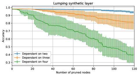
Figure 4: Accuracy loss when pruning nodes which incoming weights are linear combination of two, three and four other nodes’ weights in the same layer.

6 Conclusion

In this paper we present a data free filter pruning compression method based on the notion of lumpability. Even though we impose rigid constraints on the weights in order to obtain a reduced network, in doing so we also demonstrate how the resulting model exhibits the same exact behaviour. Regardless the limitations of our method, this work opens the door to a new research field where the aggregation techniques typical of performance evaluation are adopted in network compression, usually explored only by the machine learning community. In the future, we would like to further analyze how our algorithm works for different study cases, and in particular to test how an approximation of the linear dependence would affect the accuracy under different conditions. Another interesting experiment would be to use SVD on the fully connected layers to estimate how many vectors are linearly independent and therefore compute the reduction potentially achieved by our method, especially for quantized networks.

Acknowledgements.

This work has been partially supported by the Project PRIN 2020 “Nirvana - Noninterference and Reversibility Analysis in Private Blockchains” and by the Project GNCS 2022 “Proprietà qualitative e quantitative di sistemi reversibili”.

References

- [1] Alzetta, G., Marin, A., Piazza, C., Rossi, S.: Lumping-based equivalences in Markovian automata: Algorithms and applications to product-form analyses. Information and Computation 260, 99–125 (2018)
- [2] Ashiquzzaman, A., Van Ma, L., Kim, S., Lee, D., Um, T.W., Kim, J.: Compacting deep neural networks for light weight iot & scada based applications with node pruning. In: 2019 International Conference on Artificial Intelligence in Information and Communication (ICAIIC). pp. 082–085. IEEE (2019)
- [3] Baker, B., Gupta, O., Naik, N., Raskar, R.: Designing neural network architectures using reinforcement learning. arXiv preprint arXiv:1611.02167 (2016)
- [4] Blalock, D., Gonzalez Ortiz, J.J., Frankle, J., Guttag, J.: What is the state of neural network pruning? Proceedings of machine learning and systems 2, 129–146 (2020)
- [5] Buchholz, P.: Exact and ordinary lumpability in finite Markov chains. Journal of Applied Probability 31, 59–75 (1994)
- [6] Carroll, J.D., Chang, J.J.: Analysis of individual differences in multidimensional scaling via an n-way generalization of “eckart-young” decomposition. Psychometrika 35(3), 283–319 (1970)
- [7] Castellano, G., Fanelli, A.M., Pelillo, M.: An iterative pruning algorithm for feedforward neural networks. IEEE transactions on Neural networks 8(3), 519–531 (1997)
- [8] Dai, Z., Liu, H., Le, Q.V., Tan, M.: Coatnet: Marrying convolution and attention for all data sizes. Advances in Neural Information Processing Systems 34, 3965–3977 (2021)
- [9] Dang, T., Dreossi, T., Piazza, C.: Parameter synthesis through temporal logic specifications. In: International Symposium on Formal Methods. pp. 213–230. Springer (2015)
- [10] Deng, L., Li, G., Han, S., Shi, L., Xie, Y.: Model compression and hardware acceleration for neural networks: A comprehensive survey. Proceedings of the IEEE 108(4), 485–532 (2020)
- [11] Denton, E.L., Zaremba, W., Bruna, J., LeCun, Y., Fergus, R.: Exploiting linear structure within convolutional networks for efficient evaluation. In: Advances in neural information processing systems. pp. 1269–1277 (2014)
- [12] Elsken, T., Metzen, J.H., Hutter, F.: Neural architecture search: A survey. The Journal of Machine Learning Research 20(1), 1997–2017 (2019)
- [13] Frankle, J., Carbin, M.: The lottery ticket hypothesis: Finding sparse, trainable neural networks. arXiv preprint arXiv:1803.03635 (2018)
- [14] Han, S., Mao, H., Dally, W.J.: Deep compression: Compressing deep neural networks with pruning, trained quantization and huffman coding. arXiv preprint arXiv:1510.00149 (2015)
- [15] Han, S., Pool, J., Tran, J., Dally, W.J.: Learning both weights and connections for efficient neural networks. arXiv preprint arXiv:1506.02626 (2015)
- [16] Harshman, R.A., et al.: Foundations of the parafac procedure: Models and conditions for an” explanatory” multimodal factor analysis (1970)
- [17] He, Y., Liu, P., Wang, Z., Hu, Z., Yang, Y.: Filter pruning via geometric median for deep convolutional neural networks acceleration. In: Proceedings of the IEEE/CVF Conference on Computer Vision and Pattern Recognition. pp. 4340–4349 (2019)
- [18] Hillston, J.: A Compositional Approach to Performance Modelling. Ph.D. thesis, Department of Computer Science, University of Edinburgh (1994)
- [19] Hillston, J., Marin, A., Piazza, C., Rossi, S.: Contextual lumpability. In: Proc. of Valuetools 2013 Conf. pp. 194–203. ACM Press (2013)
- [20] Howard, A., Sandler, M., Chu, G., Chen, L.C., Chen, B., Tan, M., Wang, W., Zhu, Y., Pang, R., Vasudevan, V., et al.: Searching for mobilenetv3. In: Proceedings of the IEEE/CVF International Conference on Computer Vision. pp. 1314–1324 (2019)
- [21] Howard, A.G., Zhu, M., Chen, B., Kalenichenko, D., Wang, W., Weyand, T., Andreetto, M., Adam, H.: Mobilenets: Efficient convolutional neural networks for mobile vision applications. arXiv preprint arXiv:1704.04861 (2017)
- [22] Hu, H., Peng, R., Tai, Y.W., Tang, C.K.: Network trimming: A data-driven neuron pruning approach towards efficient deep architectures. arXiv preprint arXiv:1607.03250 (2016)
- [23] Iandola, F.N., Han, S., Moskewicz, M.W., Ashraf, K., Dally, W.J., Keutzer, K.: Squeezenet: Alexnet-level accuracy with 50x fewer parameters and¡ 0.5 mb model size. arXiv preprint arXiv:1602.07360 (2016)
- [24] Kemeny, J.G., Snell, J.L.: Finite Markov Chains. Springer (1976)
- [25] Kolesnikov, A., Beyer, L., Zhai, X., Puigcerver, J., Yung, J., Gelly, S., Houlsby, N.: Big transfer (bit): General visual representation learning. In: European conference on computer vision. pp. 491–507. Springer (2020)
- [26] Krizhevsky, A., Sutskever, I., Hinton, G.E.: Imagenet classification with deep convolutional neural networks. Advances in neural information processing systems 25 (2012)
- [27] LeCun, Y., Denker, J.S., Solla, S.A.: Optimal brain damage. In: Advances in neural information processing systems. pp. 598–605 (1990)
- [28] Li, H., Kadav, A., Durdanovic, I., Samet, H., Graf, H.P.: Pruning filters for efficient convnets. arXiv preprint arXiv:1608.08710 (2016)
- [29] Lin, M., Chen, Q., Yan, S.: Network in network. arXiv preprint arXiv:1312.4400 (2013)
- [30] Lin, M., Ji, R., Wang, Y., Zhang, Y., Zhang, B., Tian, Y., Shao, L.: Hrank: Filter pruning using high-rank feature map. In: Proceedings of the IEEE/CVF Conference on Computer Vision and Pattern Recognition. pp. 1529–1538 (2020)
- [31] Lin, S., Ji, R., Yan, C., Zhang, B., Cao, L., Ye, Q., Huang, F., Doermann, D.: Towards optimal structured cnn pruning via generative adversarial learning. In: Proceedings of the IEEE/CVF Conference on Computer Vision and Pattern Recognition. pp. 2790–2799 (2019)
- [32] Liu, Y., Sun, Y., Xue, B., Zhang, M., Yen, G.G., Tan, K.C.: A survey on evolutionary neural architecture search. IEEE transactions on neural networks and learning systems (2021)
- [33] Liu, Z., Li, J., Shen, Z., Huang, G., Yan, S., Zhang, C.: Learning efficient convolutional networks through network slimming. In: Proceedings of the IEEE international conference on computer vision. pp. 2736–2744 (2017)
- [34] Ma, N., Zhang, X., Zheng, H.T., Sun, J.: Shufflenet v2: Practical guidelines for efficient cnn architecture design. In: Proceedings of the European conference on computer vision (ECCV). pp. 116–131 (2018)
- [35] Marin, A., Piazza, C., Rossi, S.: Proportional lumpability. In: Formal Modeling and Analysis of Timed Systems - 17th International Conference, FORMATS 2019, Proceedings. Lecture Notes in Computer Science, vol. 11750, pp. 265–281. Springer (2019)
- [36] Marin, A., Piazza, C., Rossi, S.: Proportional lumpability and proportional bisimilarity. Acta Informatica 59(2), 211–244 (2022)
- [37] Molchanov, P., Mallya, A., Tyree, S., Frosio, I., Kautz, J.: Importance estimation for neural network pruning. In: Proceedings of the IEEE/CVF Conference on Computer Vision and Pattern Recognition. pp. 11264–11272 (2019)
- [38] Piazza, C., Rossi, S.: Reasoning about proportional lumpability. In: QEST. Lecture Notes in Computer Science, vol. 12846, pp. 372–390. Springer (2021)
- [39] Prabhakar, P.: Bisimulations for neural network reduction. In: International Conference on Verification, Model Checking, and Abstract Interpretation. pp. 285–300. Springer (2022)
- [40] Rastegari, M., Ordonez, V., Redmon, J., Farhadi, A.: Xnor-net: Imagenet classification using binary convolutional neural networks. In: European conference on computer vision. pp. 525–542. Springer (2016)
- [41] Ren, P., Xiao, Y., Chang, X., Huang, P.Y., Li, Z., Chen, X., Wang, X.: A comprehensive survey of neural architecture search: Challenges and solutions. ACM Computing Surveys (CSUR) 54(4), 1–34 (2021)
- [42] Ressi, D., Pistellato, M., Albarelli, A., Bergamasco, F.: A relevance-based cnn trimming method for low-resources embedded vision. In: International Conference of the Italian Association for Artificial Intelligence. pp. 297–309. Springer (2022)
- [43] Sandler, M., Howard, A., Zhu, M., Zhmoginov, A., Chen, L.C.: Mobilenetv2: Inverted residuals and linear bottlenecks. In: Proceedings of the IEEE conference on computer vision and pattern recognition. pp. 4510–4520 (2018)
- [44] Schweitzer, P.: Aggregation methods for large Markov chains. In: Proc. of the International Workshop on Computer Performance and Reliability. pp. 275–286. North Holland (1984)
- [45] Sproston, J., Donatelli, S.: Backward stochastic bisimulation in csl model checking. In: First International Conference on the Quantitative Evaluation of Systems, 2004. QEST 2004. Proceedings. pp. 220–229. IEEE (2004)
- [46] Szegedy, C., Liu, W., Jia, Y., Sermanet, P., Reed, S., Anguelov, D., Erhan, D., Vanhoucke, V., Rabinovich, A.: Going deeper with convolutions. In: Proceedings of the IEEE conference on computer vision and pattern recognition. pp. 1–9 (2015)
- [47] Szegedy, C., Vanhoucke, V., Ioffe, S., Shlens, J., Wojna, Z.: Rethinking the inception architecture for computer vision. In: Proceedings of the IEEE conference on computer vision and pattern recognition. pp. 2818–2826 (2016)
- [48] Tan, C.M.J., Motani, M.: Dropnet: Reducing neural network complexity via iterative pruning. In: International Conference on Machine Learning. pp. 9356–9366. PMLR (2020)
- [49] Tan, M., Le, Q.: Efficientnet: Rethinking model scaling for convolutional neural networks. In: International conference on machine learning. pp. 6105–6114. PMLR (2019)
- [50] Tan, M., Le, Q.V.: Efficientnetv2: Smaller models and faster training. arXiv preprint arXiv:2104.00298 (2021)
- [51] Tucker, L.R.: Some mathematical notes on three-mode factor analysis. Psychometrika 31(3), 279–311 (1966)
- [52] Wang, Z., Xie, X., Shi, G.: Rfpruning: A retraining-free pruning method for accelerating convolutional neural networks. Applied Soft Computing 113, 107860 (2021)
- [53] Xiao, L., Bahri, Y., Sohl-Dickstein, J., Schoenholz, S., Pennington, J.: Dynamical isometry and a mean field theory of cnns: How to train 10,000-layer vanilla convolutional neural networks. In: International Conference on Machine Learning. pp. 5393–5402. PMLR (2018)
- [54] Yu, J., Wang, Z., Vasudevan, V., Yeung, L., Seyedhosseini, M., Wu, Y.: Coca: Contrastive captioners are image-text foundation models. arXiv preprint arXiv:2205.01917 (2022)
- [55] Yu, R., Li, A., Chen, C.F., Lai, J.H., Morariu, V.I., Han, X., Gao, M., Lin, C.Y., Davis, L.S.: Nisp: Pruning networks using neuron importance score propagation. In: Proceedings of the IEEE conference on computer vision and pattern recognition. pp. 9194–9203 (2018)
- [56] Zhang, X., Zhou, X., Lin, M., Sun, J.: Shufflenet: An extremely efficient convolutional neural network for mobile devices. In: Proceedings of the IEEE conference on computer vision and pattern recognition. pp. 6848–6856 (2018)
- [57] Zoph, B., Le, Q.V.: Neural architecture search with reinforcement learning. arXiv preprint arXiv:1611.01578 (2016)