Phenomenological formula for Quantum Hall resistivity
based on the Riemann zeta function

Abstract

We propose a formula constructed out of elementary functions that captures many of the detailed features of the transverse resistivity $\rho_{xy}$ for the integer quantum Hall effect. It is merely a phenomenological formula in the sense that it is not based on any transport calculation for a specific class of physical models involving electrons in a disordered landscape, thus, whether a physical model exists which realizes this resistivity remains an open question. Nevertheless, since the formula involves the Riemann zeta function and its non-trivial zeros play a central role, it is amusing to consider the implications of the Riemann Hypothesis in light of it.

I Introduction

The integer quantum Hall effect (IQHE) refers to the remarkable properties of a non-interacting electron gas in two spatial dimensions in the presence of a magnetic field $B$ and a disordered potential. These properties are only observed under the extreme conditions of strong magnetic field and very low temperature which explains why it was discovered relatively late vonKlitzing . Figure 1 shows some typical experimental data. The most striking feature is the exact quantization of the transverse resistivity on the “plateaux”:

$$\rho_{xy}=\dfrac{1}{n}\,\dfrac{h}{e^{2}},~{}~{}~{}~{}n=1,2,3,\ldots$$ (1)

where $h$ is Planck’s constant and $e$ the electron charge.

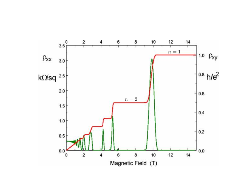
Figure 1: Experimental data on the Hall resistivity $\rho_{xy}$ as a function of magnetic field at very low temperatures (red curve, the green curve is the longitudinal $\rho_{xx}$.)

The theoretical understanding of the IQHE is by now well-developed and there are many excellent reviews and books Girvin . Some early pioneering works were by Laughlin and Halperin Laughlin ; Halperin . Let us review some of the very basics. The pure problem of a single electron in a magnetic field was solved long ago by Landau. The eigenstates fall into Laudau levels with energy $E_{L}(n)=(n+\tfrac{1}{2})\hbar eB/m$ where $m$ is the electron mass. Each Landau level has a large degeneracy of states $N_{{\rm states}}=\Phi/\Phi_{0}$ where $\Phi$ is the magnetic flux and $\Phi_{0}=hc/e$. These are all de-localized states. The IQHE is instead a many body problem, namely a finite density electron gas at finite temperature with non-zero $B$, in the presence of disorder, such as various kinds of random impurities or defects. The plateaux would not exist without this disorder and a complete understanding involves Anderson localization. Since we will not be considering any detailed physically motivated hamiltonian, let us just give a rough and brief picture of the phenomenon. At energies approximately in the gap between the pure Landau levels the states are localized due to disorder and thus don’t contribute to the conductivity and it remains constant on the plateaux. At certain critical energies $E^{c}_{n}$ near the original Landau levels, where by definition $E^{c}_{n+1}>E^{c}_{n}$, there is a quantum phase transition where some states are delocalized and contribute to a change of the conductivity. Let us write this in terms of the Fermi energy $E_{F}$:

$${\rm If}~{}~{}E^{c}_{n}>E_{F}>E^{c}_{n-1}~{}~{}~{}~{}{\rm then}~{}~{}\rho_{xy}=\dfrac{1}{n}\,\dfrac{h}{e^{2}}$$ (2)

For the experiments it is easier to control the magnetic field, thus we define critical $B^{c}_{n}$ where $B^{c}_{n+1}<B^{c}_{n}$ and:

$${\rm If}~{}~{}B^{c}_{n}<B<B^{c}_{n-1}~{}~{}~{}~{}{\rm then}~{}~{}\rho_{xy}=\dfrac{1}{n}\,\dfrac{h}{e^{2}}.$$ (3)

It will also be important to point out that the integer $n$ in the quantization of $\rho_{xy}$ was eventually understood as a topological invariant, sometimes referred to as a Chern number Thouless . This fact explains the robustness of the quantized plateaux in spite of variable details of the sample, in particular the realization of disorder, which varies from sample to sample. It is also known that the transitions between plateaux are infinitely sharp at zero temperature, and for the most part we assume we are in this situation. We wish to also mention that the IQHE also exists in models without Landau levels Haldane .

Although the theory of the IQHE is well-developed, the explicit calculation of $\rho_{xy}$ is a difficult problem since it is a transport property in the presence of disorder. One can attempt disorder averaging, however this is also notoriously difficult, especially at the critical transitions. In fact, the precise nature of the quantum critical points at the transitions remains unknown; even the delocalization exponent is only known numerically. We will consider this exponent in Section IV. Inspection of Figure 1 indicates many complicated details, such as the following. The widths of the plateaux vary considerably for a single sample, becoming smaller as $B$ is decreased. Apart from this, the critical values $B^{c}_{n}$ appear random, and certainly depend on the realization of the disorder, of which there are infinite possibilities. The resistivity vanishes at $B=0$, where it is approximately linear.

In this paper, we will merely present an explicit mathematical function that has many of the same properties as the measured $\rho_{xy}$. It is not such a simple matter to conjure up such a function, since the measured $\rho_{xy}$ has many detailed features. Our proposed formula is relatively simple, being constructed from the gamma and zeta functions, and captures many of these salient features. Hence our terminology “phenomenological”, since we don’t attempt to compute the resistivity for any specific many-body hamiltonian, which in any case is a very difficult problem due to the disorder. For these reasons, it will be left as an open question as to whether any specific model hamiltonian for the IQHE has the transport properties that correspond to our formula, even approximately. We wish to point out however that the zeta function has an integral representation involving the Fermi-Dirac distribution $1/(e^{\varepsilon}+1)$ which we recall in the Appendix (28), and this provides some encouragement that our formula may eventually be understood as a resistivity for a gas of fermions. Clearly some guesswork is involved and this exercise will not necessarily prove to be fruitful since it is not based on methods used to compute transport, such as a Kubo formula. However we wish to point out that this kind of guesswork has been proven to be successful for some well-known problems. For instance, let us just mention Veneziano’s guess of a scattering amplitude expressed only in terms of ratios of gamma functions led to the development of the huge field of string theoryVeneziano . Of course we cannot promise such success here, however we feel it is still worth pursuing.

For our proposed formula, the non-trivial zeros of the zeta function play a crucial role, and thus can perhaps provide some new insights on the Riemann Hypothesis (RH). As emphasized above, we do not know if any microscopic quantum many body model leads to a resistivity that corresponds to our phenomenological formula. Nevertheless, if we hypothesize such a connection, then the RH can be interpreted in light of it. There are very few approaches to the RH based essentially on physics, and this may be new one. We should mention approaches based on the Hilbert-Pòlya idea that perhaps there exists a single particle quantum hamiltonian whose eigenvalues are equal to the ordinates of zeros on the critical line. This has been pursued by Berry, Keating, Sierra and others BerryK ; BerryK2 ; Sierra . A very different approach is based on ideas in statistical mechanics, in particular properties of random walks, where the randomness arises from the pseudo-randomness of the prime numbers. See in particular the most recent work Mussardo and references therein. To our knowledge a possible connection between the IQHE and the RH has not been explored before, and our hope is that this short work may shed some light on at least one of them. We wish to mention though that a relation between the pure Landau problem and the Riemann zeros was proposed in SierraTownsend , however without disorder this is not the same physics as the IQHE which involves transport rather than energy eigenvalues.

II A phenomenological formula for $\rho_{xy}$

Let us straightaway present our formula. Let $s=\sigma+it$ be a complex variable and first define the real function:

$$\theta(\sigma,t)=\Im\log\Gamma(s/2)-t\,\log\sqrt{\pi}+{\rm arg}\,\zeta(s),~{}~{}~{}~{}~{}(s=\sigma+it).$$ (4)

First a few words about the components of this function, which can in fact be interpreted as an angle, as we will explain. $\Im\log\Gamma\left(\tfrac{1}{2}(\sigma+it)\right)$ should be understood as ${\rm arg}\,\Gamma(s/2)$. It is important here and elsewhere that in the above equation it is ${\rm arg}$ and not ${\rm Arg}$, where the latter by definition is the principal branch. Remind that for any meromorphic function $f(s)$, away from a zero or pole one can always calculate ${\rm Arg}\,f(s)=\arctan\,\Im f(s)/\Re f(s)$ on the principal branch $-\pi<{\rm Arg}<\pi$. On the other hand, ${\rm arg}$ keeps track of branches and needs to be defined differently, typically using piecewise integration of $f^{\prime}(s)/f(s)$ from some known point. (${\rm arg}(e^{i\alpha})=\alpha$ for $-\infty<\alpha<\infty$.) For instance for ${\rm arg}\,\zeta(\tfrac{1}{2}+it)$ one standard definition is via the contour ${\cal C}^{\prime}$ in Figure 5. In summary, if $s$ is neither a zero nor a pole, then

$${\rm arg}\,f(s)={\rm Arg}\,f(s)~{}~{}~{}{\rm mod}~{}2\pi,~{}~{}~{}~{}~{}~{}-\pi<{\rm Arg}\,f(s)<\pi,$$ (5)

however in the present context, the ${\rm mod}~{}2\pi$ will be important. The contribution from ${\rm arg}\,\Gamma$ is a smooth function that grows with $t$. Using the Stirling formula and its corrections one can easily show for large $t$:

$$\Im\log\Gamma\left(\tfrac{1}{2}(\sigma+it)\right)-t\,\log\sqrt{\pi}=\dfrac{t}{2}\log\left(\dfrac{t}{2\pi e}\right)+\dfrac{\pi(\sigma-1)}{4}-\dfrac{(3\sigma^{2}-6\sigma+2)}{12t}+{\cal O}(1/t^{3}).$$ (6)

On the other hand, ${\rm arg}\,\zeta(s)$ is a much more complicated quantity and where all the action is. Some basic facts we need about the zeta function are collected in the Appendix. There is no analog of Stirling’s formula that would lead to anything as simple as (6). An important role will be played by $S(t)={\rm arg}\,\zeta(\tfrac{1}{2}+it)/\pi$, and there is a large mathematical literature concerning it. Here let us just mention Selberg’s central limit theorem Selberg : $S(t)$ satisfies a normal distribution with zero mean and standard deviation equal to$\tfrac{1}{\sqrt{2}\pi}\sqrt{\log\log t}$ in the limit $t\to\infty$. Thus it grows very, very slowly with $t$ compared to the first terms in (4). Thus to a high probability, ${\rm arg}\,(\tfrac{1}{2}+it)$ is nearly always on the principal branch. Nevertheless it can attain infinitely large values, though very rarely, due to the tail of the normal distribution.

With these preliminaries, we present the phenomenological function we advertised. Henceforth we work in units where $h=c=1$, we set $m=e=1$, and $B$ is expressed in dimensionless units, such as $B/B_{0}$ where $B_{0}$ is a reference magnetic field strength. We first present the simplest version, and defer presenting some deformations to Section IV:

$$\rho_{xy}(B)=\dfrac{\pi}{\theta(\tfrac{1}{2},1/B)+2\pi}.$$ (7)

In Figure 2 we plot the above function, and it certainly shows some resemblance to the data in Figure 1.

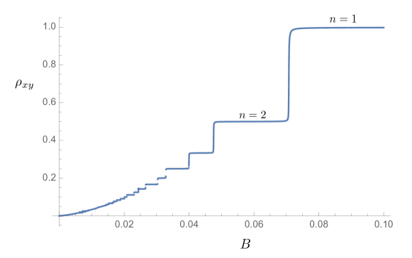
Figure 2: Plot of the function (1). We have shifted $\sigma=\tfrac{1}{2}\to\tfrac{1}{2}+\delta$ with very small positive $\delta$ in order to smooth out the transitions. At $\sigma=\tfrac{1}{2}$, the transitions are infinitely sharp as expected at zero temperature.

For fixed $B$, the Fermi energy is a function of the number density of electrons. If the density is fixed, as in a specific sample, then the Fermi energy depends on $B$, thus one can observe the plateaux by either varying $E_{F}$ or $B$. The relation between these quantities can be complicated. Note however that since the degeneracy of each pure Landau level is proportional to $B$, we roughly expect that $E_{F}\propto 1/B$. Since we will not deal with any specific material, and we are not experts, as an oversimplification we will simply define for now

$$E^{c}_{n}\equiv 1/B^{c}_{n}$$ (8)

in appropriate units. Variations of the above formula will be considered in Section IV.

Let us list some of the main features of (7):

$\bullet$    The values of the resistivity are exactly quantized as $\rho_{xy}=1/n$ on the plateaux. If one assumes the RH, and all the non-trivial zeros are simple, then this is explained by the well-known result that the number of zeros of $\zeta(s)$ inside the critical strip $0<\sigma<1$ with $0<t<T$ is given by

$$N(T)=\theta(\tfrac{1}{2},T)/\pi+1.$$ (9)

This is a consequence of Cauchy’s argument principle, and is reviewed in the Appendix.

$\bullet$    Let $\rho_{n}=\tfrac{1}{2}+it_{n}$ denote the $n$-th zero of $\zeta$ on the upper critical line, where by convention $n=1,2,\ldots$ and the first few are $t_{1}=14.134..,~{}t_{2}=21.022....$. Again assuming the RH, the critical values are given precisely by these zeros:

$$B^{c}_{n}=1/t_{n}~{}~{}\Longrightarrow~{}~{}E^{c}_{n}=t_{n}.$$ (10)

$\bullet$    The widths of the plateaux, $B^{c}_{n}-B^{c}_{n+1}$, become smaller and smaller as $B$ is decreased, which resembles the experimental data. Although we did not attempt a fit to the data in Figure 1, one can check that the ratios $B^{c}_{n+1}/B^{c}_{n}$ are roughly equal to $t_{n}/t_{n+1}$.

$\bullet$    The resistivity vanishes at $B=0$ nearly linearly:

$$\lim_{B\to 0}\rho_{xy}(B)\approx\dfrac{2\pi B}{\log(1/B)}.$$ (11)

By replacing $B$ with $B|\log(B)|$ in (7), $\rho_{xy}(B)$ is linear near $B=0$ up to much smaller $\log\log B$ corrections. We will consider other kinds of deformations in Section IV.

III Interpretation in connection with the Riemann Hypothesis

The RH is the conjecture that all zeros inside the critical strip $0<\sigma<1$ are on the critical line $\sigma=\tfrac{1}{2}$. Whether these zeros are simple or not also remains a difficult open problem. In the last section we already commented that our phenomenological formula (7) can only describe the IQHE if the RH is true and all zeros are simple. Let us elaborate. Suppose the RH is false such that there are zeros $\rho_{\bullet}$ off the line, which necessarily come in pairs $\rho_{\bullet}=\sigma_{\bullet}+it_{\bullet},1-\sigma_{\bullet}+it_{\bullet}$. These zeros contribute to $N(T)$ with multiplicity $2$ or more. This would imply that the transverse conductivity $1/\rho_{xy}$ does not always jump by $1$ at the transitions, but rather sometimes jumps by $2$, or more depending on their multiplicity. In other words not all integers $n$ in (1) would be physically realized. Furthermore, assuming the RH, if the zeros were not simple, then $n$ would not always jump by exactly $1$, but rather by the order of the zero, and again some $n$ would be absent.

In our simplified physical picture thus far, the critical energies $E^{c}_{n}$ are identified as the Riemann zeros $t_{n}$ based on (8). Whereas the quantization $n$ in (1) is robust, i.e. sample independent due to its relation to the Chern topological number, the values at the transition $E^{c}_{n}$ are not universal. They depend in particular on the realization of the disorder, i.e. details of the disorder, among other properties of the sample. A famous conjecture is that the differences between Riemann zeros $t_{n}$ satisfies the GUE statistics of random hamiltonians Montgomery ; Odlyzko . In the present context this randomness is naturally explained as arising from the random disorder. In fact random matrix theory has already been applied to quantum transport in disordered systems Beenakker . The actual Riemann zeros must then correspond to a special realization of disorder, just as the Hilbert-Pólya idea involves some as yet unknown hamiltonian. It is important then that our formula (7) can be deformed in order to accommodate for variable $E^{c}_{n}\neq t_{n}$, and other variations such as finite temperature. This will be explored in Section IV. It is interesting to note that extreme values of $|\zeta(\tfrac{1}{2}+it)|$ were studied from the perspective of the so-called freezing transition in disordered landscapes Fyodorov1 ; Fyodorov2 , and the latter is an important component of the physics of the IQHE.

Returning to pure mathematics, the angle $\theta(\sigma,t)$ contains all the information about the zeros although in a not so transparent way. This was developed in a precise manner in Gui . Referring to the completed zeta function $\chi(s)$ in (29), it is known that inside the critical strip $\chi(s)$ and $\zeta(s)$ have the same zeros. Obviously at a zero $\rho_{n}$, the modulus $|\chi(\rho_{n})|=0$, however such a formula is not very useful in enumerating the zeros. Assuming the RH, one can in fact extract the actual exact zeros $t_{n}$ from $\theta(\sigma,t)$ in the following way. First it is important that even though $|\chi(s)|=0$ at a zero, its argument $\theta(\sigma,t)$ is still well defined once one specifies a contour indicating the direction of approach to the zero. Let us provide a slightly different argument than the one presented in Gui . On the critical line $\sigma=\tfrac{1}{2}$, by the functional equation (30), $\chi(s)$ is real. If the RH is true and the zeros are simple, it must simply change sign at each zero. Thus, assuming the RH and the simplicity of the zeros, $\theta(\tfrac{1}{2},t)$ must jump by $\pi$ at each zero. Approaching zeros along the critical line from below, one finds

$$\lim_{\epsilon\to 0^{+}}\,\theta(\tfrac{1}{2},t_{n}-\epsilon)=\pi(n-1).$$ (12)

Rotating counterclockwise by $\pi/2$, one deduces

$$\lim_{\delta\to 0^{+}}\,\theta(\tfrac{1}{2}+\delta,t_{n})=\pi(n-\tfrac{3}{2}).$$ (13)

The above equation was used in Gui to calculate zeros to very high accuracy. It fact it was proven that if there is a unique solution to (13) for every $n$, then the RH is true and all zeros are simple. The importance of approaching the zeros from the right of the critical line is two-fold. For so-called $L$-functions based on non-principal Dirichlet characters, there are strong arguments that the Euler product formula (EPF) converges for $\sigma>\tfrac{1}{2}$ (See LM1 ). For zeta itself, the Euler product formula is

$$\zeta(s)=\prod_{p}\left(1-\dfrac{1}{p^{s}}\right)^{-1}$$ (14)

where $p$ is a prime, and the EPF converges only for $\sigma>1$, unlike what is expected for $L$-functions based on non-principal Dirichlet characters. To the left of the critical line, ${\rm arg}\,\zeta(s)$ behaves quite differently than from the right: from equation (33) one sees that to the left there are many more changes of branch compared with to the right. In conjunction with the EPF, one can use the latter to approximate ${\rm arg}\,\zeta(\tfrac{1}{2}+it)$ and thereby compute the zeros $t_{n}$ directly from the prime numbers with a truncation of the EPF, at least approximately ALzeta .

IV Deformations of the formula for $\rho_{xy}$: variable $B^{c}_{n}$ and modeling finite temperature

As explained above, we interpreted the critical $E^{c}_{n}$ as equal to the exact Riemann zeros on the critical line. In reality, for a specific experimental sample, these $E^{c}_{n}$ are not equal to the exact Riemann zeros $t_{n}$. It is thus important for our proposal that the $E^{c}_{n}$ can be deformed away from the exact and known $t_{n}$ without spoiling the exact quantization of $n$ in (1). One expects this is possible since $n$ is topological. This can be done in many ways, and in this section we explore a few.

$\bullet$    Deforming the functional dependence on $B$.    The most straightforward deformation is to change the function of $B$ inside $\theta(\tfrac{1}{2},1/B)$ in (7), i.e. to replace $1/B$ by a function $f(B)$. The resistivity remains quantized on the plateaux, i.e. equation (1) still holds. However this modifies the critical values $B^{c}_{n}$ to solutions of $f(B^{c}_{n})=t_{n}$. For instance, changing $1/B$ by a constant $\alpha/B$ simply rescales the $B^{c}_{n}$. More importantly, replacing $1/B$ with $f(B)=1/B|\log B|$ makes the small $B$ behavior much more linear near $B=0$ as previously stated.

$\bullet$    Deforming the relation between $E_{F}$ and $B$.    The proposed relation $\eqref{EBprop}$ was an over simplification of the physics, and was simply taken as a definition of $E^{c}_{n}$. Clearly the relation $E^{c}_{n}=1/B^{c}_{n}$ can be deformed, which again does not spoil the quantization on the plateaux but modifies $E^{c}_{n}$.

$\bullet$    Modeling the effect of finite temperature.    At zero temperature ${\bf T}$ the jumps at the transitions in $\rho_{xy}$ are known to be infinitely sharp, i.e. are close to step functions. At finite temperature these sharp transitions are broadened smoothly and have a finite width. It is known experimentally that the jumps are still centered around the zero temperature $B^{c}_{n}$ but deformed in a smooth way that is symmetric about $B^{c}_{n}$. This behavior can be incorporated in a relatively simple way that we now describe. In finding this deformation we were motivated by a deformation of an integral representation of the zeta function that closely resembles adding a chemical potential to the Fermi-Dirac distribution. Namely:

$$-\Gamma(s)\,{\rm Li}_{s}(-e^{-\mu})=\int_{0}^{\infty}d\varepsilon\,\varepsilon^{s-1}\dfrac{1}{e^{\varepsilon+\mu}+1},~{}~{}~{}~{}~{}~{}~{}\Re(s)>0,$$ (15)

where ${\rm Li}_{s}(z)$ is the polylogarithm:

$${\rm Li}_{s}(z)=\sum_{n=1}^{\infty}\dfrac{z^{n}}{n^{s}}$$ (16)

(analytically continued). In the above formula $\varepsilon^{s-2}$ can perhaps be viewed as a kind of density of states. The above formula applied to a free gas of fermions would identify $\mu$ as minus the chemical potential divided by the temperature, however this does not necessarily correspond to the physical situation here. It does however suggest to replace $\zeta(s)$ in (4) by the polylogarithm

$$\theta_{\mu}(\sigma,t)=\Im\log\Gamma(s/2)-t\,\log\sqrt{\pi}+{\rm arg}\,{\rm Li}_{s}(e^{-\mu}).$$ (17)

($s=\sigma+it$). Note that ${\rm Li}_{s}(1)=\zeta(s)$. Let us thus consider the deformation:

$$\rho_{xy}(B,\mu)=\dfrac{\pi}{\theta_{\mu}(\tfrac{1}{2},1/B)+2\pi}.$$ (18)

The resulting resistivity closely captures the broadening of the transitions found in the experimental data, as seen in Figure 3.

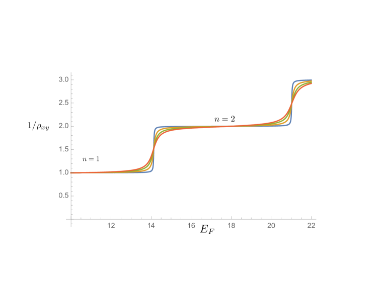
Figure 3: The conductivity $1/\rho_{xy}$ in (18) with $\mu=0.01,0.05,0.10,0.15$.

It is then interesting to see what (18) implies for the de-localization exponent $\nu$. At the transition the correlation length diverges $\xi_{c}\sim|x-x_{c}|^{-\nu}$ where $x$ could be the magnetic field for instance. The broadening of the transition at finite temperature depends on $\nu$. At zero temperature ${\bf T}$ the transition is sharp, thus $d\rho_{xy}/dB$ diverges. It is known from the physics that (see for instance RIMS ):

$$\dfrac{\partial\rho_{xy}}{\partial B}\Big{|}_{B=B^{c}_{n}}\sim{\bf T}^{-\kappa}$$ (19)

where $\kappa=1/(\nu\,z)$. Here $z$ is the dynamical exponent that relates temperature and phase coherence length $\ell_{\phi}\sim T^{-1/z}$. For relativistic systems $z=1$ and it is known that for the IQHE $z\approx 1$. From the formula (18) one sees that the sharpness of the transition is controlled by $\mu$, where the derivative in (19) is infinite when $\mu=0$. At the $n$-th transition around $\mu=0$, from the formula (18) the simple exponent $\kappa=1$ is obtained:

$$\dfrac{\partial\rho_{xy}}{\partial B}\Big{|}_{B=B^{c}_{n}}=C_{n}\,\mu^{-\kappa},~{}~{}~{}~{}~{}\kappa=1.$$ (20)

The exponent $\kappa$ is the same for all $n$ but $C_{n}$ varies, for instance $C_{1}=17.46,C_{2}=11.59$. Experimentally $\nu\approx 2.38$ whereas relatively recent analysis of the Chalker-Coddington network model gives $\nu=2.59$ RIMS . Based on the formula (18) we can obtain non-trivial $\kappa\neq 1$ by simply replacing $\mu$ by $\mu^{\kappa}$.

$\bullet$    A deformation of the actual Riemann zeros.    There is another interesting deformation which is rather different than the above which involves deforming the $\tfrac{1}{2}$ in $\theta(\tfrac{1}{2},1/B)$ in (7), as we now explain. From $\overline{\chi(s)}=\chi(\overline{s})$ one has $\theta(\sigma,-t)=-\theta(\sigma,t)$  ${\rm mod}~{}2\pi$. Combined with the functional equation (32), one has

$$\theta(\sigma,t)+\theta(1-\sigma,t)=0,~{}~{}~{}~{}~{}{\rm mod}~{}2\pi.$$ (21)

Let us then define

$$\theta_{S}(\sigma,t)\equiv\tfrac{1}{2}\left(\theta(\sigma,t)+\theta(1-\sigma,t)\right).$$ (22)

We can thus define what is necessarily an integer $\mathfrak{n}(\sigma,t)$ for all $\sigma,t$:

$$\mathfrak{n}(\sigma,t)=\theta_{S}(\sigma,t)/\pi+1.$$ (23)

Let us then deform $\rho_{xy}$ as follows:

$$\rho_{xy}(B,\sigma)=\dfrac{\pi}{\theta_{S}(\sigma,1/B)+2\pi}.$$ (24)

When $\sigma=\tfrac{1}{2}$,  $\mathfrak{n}(\tfrac{1}{2},T)$ equals the number of zeros along the critical line $N(T)$ in eq. (9) (assuming RH). We have observed an interesting mathematical property: $\mathfrak{n}(\sigma,T)$ is also equal to $N(T)$ for continuous $\sigma\neq\tfrac{1}{2}$ but with small deformations of the transition values $t_{n}\to\widehat{t}_{n}$ that depend on $\sigma$ and $n$. The deformed $\widehat{t}_{n}$ are clearly no longer zeros of $\zeta$. One explanation for this property is that small deformations from $\sigma=\tfrac{1}{2}$ should not change $N(t)$ as long as one is on a plateaux and not too close to the transition, however we have no proof of this. More precisely $\mathfrak{n}(\sigma,T)=N(T)$ for $T$ deep inside the plateaux away from the transitions. We have verified this for $n$ up to $1000$. In other words this deformation of $\sigma$ from $\tfrac{1}{2}$ does not change the topological number $n$ on the plateaux, however the critical values $E^{c}_{n}$ are slightly deformed from $t_{n}$ in a non-trivial manner. This is only true for $\sigma$ not very large, otherwise the counting is affected by the poles of $\chi(s)$ at the poles of $\Gamma(s/2)$. Thus in such a deformation one should limit $-1<\sigma<2$, which includes values outside the critical strip. We show this numerically in Figure 4 around the first zero $t_{1}=14.1347..$ for the extreme deformation $\sigma=2$. One sees that $t_{1}$ is deformed to approximately $\widehat{t}_{1}=14.42$. It is somewhat remarkable that the function $\theta_{S}(\sigma,t)$ knows about $N(T)$ on the plateaux even though it can be computed from $\zeta$ for values completely outside the critical strip $\sigma>1$. This perhaps has some interesting implications in analytic number theory.

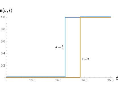
Figure 4: $N(t)=\mathfrak{n}(\sigma=\tfrac{1}{2},t)$ (blue line) verses $\mathfrak{n}(\sigma=2,t)$ (yellow line) as a function of $t$ around the first zero $t_{1}=14.1347..$. For $\mathfrak{n}(2,t)$ one sees that the plateaux values have not changed, i.e. are still $0$ or $1$, however the transition is deformed away from the actual Riemann zero $t_{1}=14.13..$ to $14.42..$.

$\bullet$    Deformations based on other $L$-functions.   On the more exotic side, in analytic number theory there are an infinite number of known $L$-functions that are expected to satisfy the so-called Grand Riemann Hypothesis, in particular those based on Dirichlet characters or on modular forms Apostol . Replacing $\theta$ in (7) with the argument of the completion of such an $L$-function analogous to (29), which is known to also involve the gamma function Apostol , one still has a robust quantization for $\rho_{xy}$, however the $t_{n}$ and thus the $B^{c}_{n}$ and $E^{c}_{n}$ are different in a non-smooth way.

V Closing remarks

We have proposed a phenomenological formula for the transverse resistivity for the IQHE built from the gamma and zeta functions which appear to capture the main physical properties at least qualitatively. The physics is very speculative: we emphasize once again that we have not performed any computation of the resistivity in any specific quantum many-body problem whatsoever, thus the main open question is whether a physical model exists that has a resistivity corresponding to our proposed formula. If we simply assume the formula we proposed for $\rho_{xy}$, then the non-trivial Riemann zeros play an essential role, and this perhaps offers a new perspective on the Riemann Hypothesis which we have partially explored. For instance, if the RH were false, then not all integers $n$ in the quantization (1) would be physically realized. All of the pure mathematics we have used is well-known, except for the discussion surrounding (24).

A common link between the IQHE and the Riemann zeros perhaps comes from random matrix theory, since the latter has been applied to both the Riemann zeros and to disordered systems. This is an appealing connection, to be contrasted to the hamiltonians proposed toward a realization of the Hilbert-Pólya idea. Proposals such as $H=xp$ and variations are not random hamiltonians; instead the randomness of the zeros is attributed to the chaotic behavior of such hamiltonians BerryK , which is very different than a particle moving in a random landscape, such as in the IQHE. In fact, relatively recently, random matrix theory was applied to a study of the extreme values of the zeta function on the critical line by making an analogy with the so-called freezing transition in disordered landscapes Fyodorov1 ; Fyodorov2 , and such a freezing transition is expected to play a role in the IQHE in order to understand its multi-fractal properties.

VI Acknowledgements

We wish to thank Giuseppe Mussardo and Germàn Sierra for discussions.

Appendix A Some basic properties of the Riemann zeta function

In this Appendix we summarize some of the fundamental properties of the zeta function that we need Edwards . Adopting standard notations in analytic number theory, throughout $s=\sigma+it$ is a complex variable.

The zeta function was originally defined by the series

$$\zeta(s)=\sum_{n=1}^{\infty}\dfrac{1}{n^{s}},~{}~{}~{}~{}~{}~{}\sigma>1$$ (25)

which converges for $\sigma>1$. It can be analytically continued to the entire complex plane where it has a simple pole at $s=1$. It has trivial zeros at $s=-2m$, $m=0,1,2,\ldots$. It is known to have an infinite number of zeros inside the “critical strip” $0<\sigma<1$. It is also known there are an infinite number of zeros along the “critical line” $\sigma=\tfrac{1}{2}$. The Riemann Hypothesis is the statement that the latter are the only zeros inside the critical strip. We label those on the upper critical line as $\rho_{n}=\tfrac{1}{2}+i\,t_{n}$, $t_{n}>0$:

$$\zeta(\rho_{n})=0,~{}~{}~{}\rho_{n}=\tfrac{1}{2}+i\,t_{n},~{}~{}~{}~{}n=1,2,3,\ldots$$ (26)

The property $\overline{\zeta(s)}=\zeta(\overline{s})$ implies $\overline{\rho_{n}}=\tfrac{1}{2}-it_{n}$ is also a zero.

It is perhaps worth pointing out that Riemann first performed the analytic continuation based on an integral representation for $\sigma>1$ involving the Bose-Einstein distribution:

$$\Gamma(s)\,\zeta(s)=\int_{0}^{\infty}\,d\varepsilon\,\varepsilon^{s-2}\,\left(\dfrac{\varepsilon}{e^{\varepsilon}-1}\right),~{}~{}~{}~{}~{}\Re(s)>1.$$ (27)

The integration contour can be deformed such that $\zeta(s)$ is defined everywhere in the complex plane, except at the pole at $s=1$. There exists another integral representation involving the Fermi-Dirac distribution:

$$\left(1-2^{1-s}\right)\,\Gamma(s)\,\zeta(s)=\int_{0}^{\infty}\,d\varepsilon\,\varepsilon^{s-2}\,\left(\dfrac{\varepsilon}{e^{\varepsilon}+1}\right),~{}~{}~{}~{}~{}\Re(s)>0,$$ (28)

which motivated some results in Section IV.

Let us define a completed zeta function as follows:

$$\chi(s)\equiv\pi^{-s/2}\,\Gamma(s/2)\,\zeta(s).$$ (29)

It satisfies the important functional equation:

$$\chi(s)=\chi(1-s).$$ (30)

This implies that zeros off the critical line necessarily come in pairs symmetric about $\tfrac{1}{2}$; namely if $\rho_{\bullet}=\sigma_{\bullet}+it_{\bullet}$ is a zero, then so is $\rho_{\bullet}=1-\sigma_{\bullet}+it_{\bullet}$.

The angle $\theta(\sigma,t)$ defined in (4) is simply its argument:

$$\theta(\sigma,t)={\rm arg}\,\chi(\sigma+it).$$ (31)

One property we will need is

$$\theta(\sigma,t)=\theta(1-\sigma,-t)$$ (32)

which follows from the functional equation. From this, one can see that ${\rm arg}\,\zeta(s)$ behaves very differently to the right verses to the left of the critical line. Using the Stirling formula, in the limit of large $t$ one has

$${\rm arg}\,\zeta(1-\sigma+it)=-{\rm arg}\,\zeta(\sigma+it)-t\log\left(t/2\pi e\right)+\dfrac{\pi}{4}+\dfrac{(6\sigma^{2}-6\sigma+1)}{12t}+{\cal O}(1/t^{3})$$ (33)

(${\rm mod}~{}2\pi$).

Cauchy’s argument principle determines the number of zeros in the critical strip with ordinate $0<t<T$, commonly referred to as $N(T)$ in the mathematics literature. Recall

$$\dfrac{1}{2\pi i}\oint_{\cal C}\dfrac{\chi^{\prime}(s)}{\chi(s)}\,ds=N_{{\rm zeros}}-N_{{\rm poles}}$$ (34)

where the number of zeros $N_{{\rm zeros}}$ includes their multiplicity, and the number of zeros $N_{{\rm poles}}$ includes their order. One has

$$\dfrac{1}{2\pi i}\oint_{\cal C}\dfrac{\chi^{\prime}(s)}{\chi(s)}\,ds=\dfrac{1}{2\pi}\oint_{\cal C}\,d\theta(s).$$ (35)

The contour ${\cal C}$ chosen is shown in Figure 5. One need only consider the part of the contour ${\cal C}^{\prime}$ to the right of the critical line by virtue of (32). In this way one obtains the formula (9) for $N(T)$. The shift by $1$ is due to the simple pole at $s=1$. This formula is only valid if $T$ is not the ordinate of a zero.

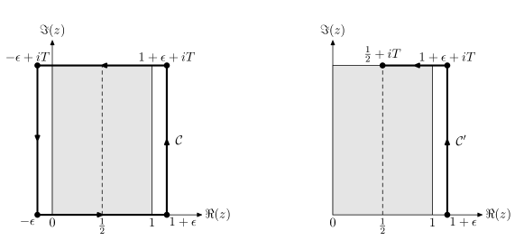
Figure 5: Left:. The contour ${\cal C}$ for the argument principle used to determine the number of zeros in the critical strip with $0<t<T$ referred to as $N(T)$ in (9). (In this figure, the complex variable $s$ is denoted as $z$.) The critical line $\sigma=\tfrac{1}{2}$ splits the rectangle in half. Right: It is sufficient to double the result for the contour ${\cal C}^{\prime}$ due to (21).

References

- (1) K. v. Klitzing, G. Dorda, and M. Pepper, New method for high-accuracy determination of the fine-structure constant based on quantized Hall resistance, Phys. Rev. Lett. 45 (6): 494 (1980).
- (2) R.E.Prange and S.M. Girvin, The Quantum Hall Effect, 1987.
- (3) R. B. Laughlin, Quantized Hall conductivity in two dimensions, Phys. Rev. B. 23 (10): 5632. (1981).
- (4) B. Halperin, Quantized Hall conductance, current-carrying edge states, and the existence of extended states in a two-dimensional disordered potential, Phys. Rev. B 25, 2185 (1982).
- (5) D. J. Thouless, M. Kohmoto, P. Nightingale, and M. den Nijs, Quantized Hall conductance in a two-dimensional periodic potential, Phys. Rev. Lett. 49 405 (1982).
- (6) F.D.M. Haldane, Model for a Quantum Hall Effect without Landau Levels: Condensed-Matter Realization of the “Parity Anomaly”, Phys. Rev. Lett. 61 (18) (1988) 2015.
- (7) G. Veneziano, Construction of a crossing-symmetric, Regge behaved amplitude for linearly rising trajectories, Nuovo Cim. A 57 (1968) 190.
- (8) D. Schumayer and D.A.W. Hutchinson, Physics of the Riemann Hypothesis, Rev. Mod. Phys. 83, 307 (2011), arXiv:1101.3116 [math-ph], and references therein.
- (9) M. V. Berry and J. P. Keating, The Riemann zeros and eigenvalue asymptotics, SIAM Review Vol. 41 (1999).
- (10) M. V. Berry and J. P. Keating, A compact hamiltonian with the same asymptotic mean spectral density as the Riemann zeros, J. Phys. A: Math. Theor. 44, 285203 (2011), and references therein.
- (11) G. Sierra, The Riemann zeros as spectrum and the Riemann hypothesis, Symmetry 2019, 11(4), 494, arXiv:1601.01797 [math-ph], and references therein.
- (12) G. Sierra and P.K. Townsend, The Landau model and the Riemann zeros, Phys. Rev. Lett. 101, 110201 (2008); arXiv:0805.4079.
- (13) G. Mussardo and A. LeClair, Randomness of Möbius coefficents and brownian motion: growth of the Mertens function and the Riemann Hypothesis, J. Stat. Mech. (2021) 113106, arXiv:2101.10336 [math.NT], and references therein.
- (14) A. Selberg, Contributions to the theory of the Riemann zeta-function. Arch. Math. Naturvid., 48(5): 89-155, (1946).
- (15) C.W. Beenakker, Random-matrix theory of quantum transport, Rev. Mod. Phys. 69 (1997) 731.
- (16) G. França and A. LeClair, Transcendental equations satisfied by the individual zeros of Riemann zeta, Dirichlet and modular L-functions, Communications in Number Theory and Physics, Vol. 9 (2015) p1, arXiv:1307.8395 [math.NT].
- (17) A. LeClair and G. Mussardo, Generalized Riemann Hypothesis, Time Series and Normal Distributions, J. Stat. Mech. 023203 (2019), arXiv:1809.06158 [math.NT] and references therein.
- (18) A. LeClair, Riemann Hypothesis and Random Walks: the Zeta case, Symmetry 2021, 13, 2014, arXiv:1601.00914 [math.NT].
- (19) K. Slevin and T. Ohtsuki, Critical exponent for the quantum Hall transition, Phys. Rev. B 80 (2009) 041304, and references therein.
- (20) T. M. Apostol, Introduction to Analytic Number Theory, Springer, NY, 1976.
- (21) H. L. Montgomery, The pair correlation of zeros of the zeta function, Analytic number theory, Proc. Sympos. Pure Math., XXIV, Providence, R.I.: American Mathematical Society, Vol. 24 (1973) 181.
- (22) A.M. Odlyzko, On the distribution of spacings between zeros of the zeta function, Mathematics of Computation, American Mathematical Society, 48(177), 273 (1987).
- (23) Y. V. Fyodorov, G. A. Hiary and J. P. Keating, Freezing Transition, Characteristic Polynomials of Random Matrices, and the Riemann Zeta Function, Phys. Rev. Lett 108 (2012) 170601 [arXiv:1202.4713].
- (24) Y. V. Fyodorov and J. P. Keating, Freezing Transitions and Extreme Values: Random Matrix Theory, , and Disordered Landscapes, Phil. Trans. Roy. Soc. A 372 (2014) 20120503 [arXiv:1211.6063].
- (25) H.M. Edwards, Riemann Zeta Function, Academic Press, New York, 1974.