An electromagnetic way to derive basic relativistic transformations

Abstract

We derive the relativistic velocity addition law, the transformations of electromagnetic fields and space-time intervals by examining the drift velocities in a crossed electromagnetic field configuration. The postulate of light velocity invariance is not taken as a priori, but is derived as the universal upper limit of drift velocities. The key is that a physical drift motion of either an electric charge or a magnetic charge remains a drift motion by any inertial reference frame transformations. Such a simple fact is incompatible with the Galilean velocity addition. This derivation provides a way to introduce relativity via elementary electromagnetism.

As is well known that the discovery of relativity was motivated by examining how the electromagnetic laws transform in different inertial frames einstein1905 . As Einstein recalled in his autobiography, he was considering a Gedanken experiment of chasing light: If one could travel at the light velocity, the electromagnetic wave would become a static field configuration, which is incompatible with the Maxwell equations einstein1951 ; norton2004 . Nevertheless, relativity is often taught in Mechanics in General Physics kittle1973 ; feynman2011 . The derivation of Lorentz transformation of space-time coordinates is typically based on two postulates: I) The relativity principle and II) the invariance of the light velocity. The former is a generalization of the Galilean transformation from mechanical laws to all physical laws including electromagnetic ones, which is natural. Nevertheless, although the light velocity invariance origins from the invariance of the Maxwell equations, it looks mysterious and unnatural.

Significant progresses have appeared in deriving relativity without light in literature levyleblond1976 ; mermin1984 ; singh1986 ; pelissetto2015 . Without loss of generality, consider the space-time transformation in 1+1 dimensions. Based on assumptions such as the homogeneity, smoothness, and isotropy of space time, it can be derived that only the Lorentz, Galilean, and rotation-like transformations are possible. They correspond to the hyperbolic, parabolic, and elliptic subgroups of SL$(2,R)$, respectively. Only the Lorentz and Galilean transformations meet the requirement of causality. If instantaneous interactions are further abandoned, then Lorentz transformation is the only choice.

There have also been signficant efforts in elucidating the intimate relation between relativity and electromagnetism in general physics instructions. The excellent textbook by E. M. Purcell, i.e., Berkely Physics Course, Vol II, formulated magnetism as the relativistic consequence of electricity. Impressively, the magnetic field given by Ampere’s law is consistent with the result by applying the inertial frame transformation to an electrostatic field as it should be. Since magnetism is our daily life experience, this is convincing for beginning students to accept relativity heartily.

In this article, we provide a new pedagogical way to re-derive relativistic transformations via elementary electromagnetism without the Maxwell equations. Even the simple phenomenon of the drift velocity in a crossed electric and magnetic field configuration, which is typically a high school textbook problem, is incompatible with the Galilean space-time transformation. The postulate of light velocity invariance is not taken for granted, but is derived as the upper limit of drift velocities. Simply by examining the transformations of drift velocities in inertial reference frames, the transformation laws of electromagnetic fields and the addition law of velocities appear naturally, which are in contradiction to the Galilean transform. This would stimulate one to re-examine the space-time coordinate transformation, which yields the Lorentz transformation. This is a logically natural way to start learning relativistic physics.

We warm up by reviewing elementary electromagnetism. Consider a crossed field configuration in an inertial reference frame $F$ as shown in Fig. 1. Without loss of generality, it is assumed that

$$\mathbf{B}=B_{z}\hat{z},\ \,\ \,\mathbf{E}=E_{y}\hat{y}.$$ (1)

For a charged particle $q$, its electric force and magnetic force (Lorentz force) are expressed by

$$\mathbf{F}_{q}=q\left(\mathbf{E}+\frac{\mathbf{v}}{c}\times\mathbf{B}\right).$$ (2)

The theory of electromagnetism actually allows the existence of magnetic monopoles dirac1931 ; schwinger1968 , although it remains elusive in experimental detections cabrera1982 . For a monopole carrying a magnetic charge $g$, its magnetic force and electric force are expressed jackson1998 by

$$\mathbf{F}_{g}=g\left(\mathbf{B}-\frac{\mathbf{v}}{c}\times\mathbf{E}\right),$$ (3)

where the electric force becomes the Lorentz one. Compared to Eq. 2, the electric Lorentz force exhibits an opposite sign, whose physical meaning is explained in Appendix A.

We use the Gaussian unit enjoying the advantage that electricity and magnetism are formulated in a symmetric way. If in the SI unit, the force formulae are

$$\mathbf{F}_{q} = q\left(\mathbf{E}+\mathbf{v}\times\mathbf{B}\right),$$

$$\mathbf{F}_{g} = g\left(\mathbf{B}-\mu_{0}\epsilon_{0}\mathbf{v}\times\mathbf{E}\right)=g\left(\mathbf{B}-\frac{\mathbf{v}}{c^{2}}\times\mathbf{E}\right).$$ (4)

So far, $c$ is just a quantity carrying the unit of velocity.

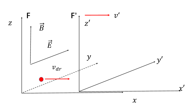
Figure 1: Transformations of a crossed electric and magnetic field configuration. In the frame $F$, the magnetic field $\mathbf{B}$ is along the $z$-direction, and the electric field $\mathbf{E}$ is along the $y$-direction. $v_{dr}$ along the $x$-direction is the drift velocity of a charge ($v_{q}$) or a monopole ($v_{g}$) defined in Eq. 5 and Eq. 6, respectively. The frame $F^{\prime}$ is moving relative to frame $F$ at the velocity of $v^{\prime}$ along the $x$-direction.

Based on Eq. 2 and Eq. 3, there exist drift velocities. For the charge $q$, its charge drift velocity is

$$\frac{v_{q}}{c}=\frac{E_{y}}{B_{z}},$$ (5)

at which the Lorentz force balances the electric force such that the charged $q$ moves in a uniform velocity along a straight line. Similarly, the monopole drift velocity for the magnetic charge $g$ is

$$\frac{v_{g}}{c}=\frac{B_{z}}{E_{y}}.$$ (6)

We define that a velocity $v$ is “physical” if it can be taken as the drift velocity for a charge or a monopole in a physically realizable crossed electromagnetic field configuration. Otherwise, it is “unphysical”. When a charge or a monopole takes a physical drift velocity, a co-moving frame can be defined in which the charge or monopole is at rest. Since velocity starts from zero continuously, when a drift velocity approaches zero, it should be physical without question. We assume that if a velocity $v$ is already physical, any velocity $u$ satisfying $|u|\leq|v|$ is also physical.

We show that the at least one of charge drift velocity $v_{q}$ (Eq. 5) and monopole drift velocity $v_{g}$ (Eq. 6) is unphysical. Contradiction would appear if both were physical. Consider the co-moving frame $F_{dr}$ with the charge drift velocity $v_{q}$. In such a frame, the charge is at rest, hence, both the magnetic force and the electric force should vanish. This means that the electric field is zero but the magnetic field does not. Otherwise, if both of them are zero in $F_{dr}$, they should remain zero in the lab frame. Then bring a magnetic charge $g$ in $F_{dr}$. It would undergo acceleration, which cannot be removed by any inertial frame transformation. On the other hand, in the co-moving frame $F^{\prime}_{dr}$ with a monopole at the drift velocity $v_{g}$, the monopole would be at rest, showing the contradiction.

Since velocity $v$ is continuous, the physical and unphysical regions should be separated by a threshold value $v_{th}$, such that $v$ is physical if $|v|<v_{th}$ and unphysical if $|v|>v_{th}$. It is easy to prove that $v_{th}\leq c$. If it were not the case, i.e, $v_{th}>c$, a set of values of $E_{y}$ and $B_{z}$ could be taken such that $1<|B_{z}/E_{y}|<v_{th}/c$. A charge would move with the drift velocity $v_{q}$, and a monopole would move with the drift velocity $v_{g}$, and both would be physical, which is impossible as shown before.

Let us check the limit of $|E|\ll|B|$. The charge drift velocity $v_{q}\ll c$, which is physical. In contrast, $v_{g}\gg c\geq v_{th}$, hence, the magnetic drift velocity is unphysical. Similarly, in the limit of $|E|\gg|B|$, the magnetic drift velocity is physical, while the electric one is unphysical.

We can prove that it is impossible for $v_{th}<c$ either. Otherwise, $v_{th}$ is non-universal, i.e., it takes different values in different inertial frames. This would be in contradiction to the relativity principle, since its different values could be used to distinguish inertial frames. This can be done by checking the transformation of $v_{th}$ in different frames (Eq. 36), which will be derived later.

As a preparation, we derive the transformations of electric and magnetic fields between different inertial frames. The key idea of reasoning would be based on the relativity principle – all inertial frames are equivalent. A physical drift motion is a uniform motion along a straight line, hence, any inertial frame transformation does not change this nature. In other words, if the electric and magnetic forces are balanced in one frame, they are balanced in any other reference frames.

Without loss of generality, the frame $F^{\prime}$ is assumed moving with a velocity $v^{\prime}$ along the $x$-axis with respect to the frame $F$. These two frames share an O(2) symmetry, i.e, the rotation symmetry with respect to the boost axis, i.e., the $x$-axis, and the reflection symmetry with respect to any plane perpendicular to the $yz$-one. The longitudinal components of the electric and magnetic fields, i.e., $E_{x}$ and $B_{x}$, are rotationally invariant. But they transform differently under the mirror reflection with respect to the $xz$-plane. Hence, each of them transform to itself without mixing. After boosting, $E_{x}$ can only change by a factor $\lambda$. On the other hand, this factor should be independent of the boosting direction. If we perform one boost transformation, and then reverse the boost back to the original frame, $\lambda^{2}=1$ is arrived. Since a boost can start with an infinitesimal velocity,

$$\lambda=1.$$ (7)

A similar reasoning can be applied to $B_{x}$. Hence, the longitudinal components of $\mathbf{E}$ and $\mathbf{B}$ are invariant

$$E_{x}^{\prime}=E_{x},~{}~{}B_{x}^{\prime}=B_{x}.$$ (8)

As for the transverse components, $B_{z}$ and $E_{y}$ are odd under the reflection with respect to the $xz$-plane, and even under the reflection with respect to the $xy$-plane. In contrast, $B_{y}$ and $E_{z}$ transform oppositely under mirror reflections with respect to these two planes. Hence, $B_{z}$ and $E_{y}$ transform into each other under the Lorentz boost, so does $B_{y}$ and $E_{z}$.

Now we assume the transformation between $E_{y}$ and $B_{z}$ as follows

$$\left(\begin{array}[]{c}E_{y}^{\prime}\\ B_{z}^{\prime}\end{array}\right)=\left(\begin{array}[]{cc}a&b\\ c&d\end{array}\right)\left(\begin{array}[]{c}E_{y}\\ B_{z}\end{array}\right),$$ (15)

where the matrix elements only depend on the boost velocity $v^{\prime}$. We choose a configuration that $E_{y}/B_{z}=v^{\prime}/c=\beta^{\prime}$ in the $F$ frame, such that the charge drift velocity $v_{q}=v^{\prime}$. In the $F^{\prime}$ frame, the electric field should vanish, i.e., $E_{y}^{\prime}=0$, then

$$\frac{b}{a}=-\frac{E_{y}}{B_{z}}=-\beta^{\prime}.$$ (16)

Similarly, a configuration that $B_{z}/E_{y}=\beta^{\prime}$ is chosen in the $F$ frame. In this case, the $F^{\prime}$ frame is just the co-moving frame of a magnetic charge with the drift velocity $v_{g}=v^{\prime}$. Consequently $B_{z}^{\prime}=0$ in the $F^{\prime}$, yielding that

$$\frac{c}{d}=-\frac{B_{z}}{E_{y}}=-\beta^{\prime}.$$ (17)

Now let us consider a general charge drift velocity $v$ in the $F$-frame with the corresponding electric and magnetic fields $B_{z}$ and $E_{y}$ such that $\beta=v/c=E_{y}/B_{z}$. Under a Lorentz boost with velocity $\beta^{\prime}=v^{\prime}/c$, the charge remains a drift motion. The drift velocity $u$ in frame $F^{\prime}$ is

$$\frac{u}{c}=\frac{E_{y}^{\prime}}{B_{z}^{\prime}}=\frac{aE_{y}+bB_{z}}{cE_{y}+dB_{z}}=\frac{a}{d}\frac{\beta-\beta^{\prime}}{1-\beta\beta^{\prime}}.$$ (18)

Similarly, we can also prepare a monopole with the same drift velocity $v$ in the $F$-frame, and choose the crossed field configuration with $B_{z}/E_{y}=v/c=\beta$. Again by the same Lorentz boost, the drift velocity becomes $u$ in frame $F^{\prime}$, then

$$\frac{u}{c}=\frac{B_{z}^{\prime}}{E_{y}^{\prime}}=\frac{cE_{y}+dB_{z}}{aE_{y}+bB_{z}}=\frac{d}{a}\frac{\beta-\beta^{\prime}}{1-\beta\beta^{\prime}}.$$ (19)

Comparing Eq. 18 with Eq. 19, $(a/d)^{2}=1$ is arrived. Since $u/c=\beta$ in the limit of $\beta^{\prime}=0$, we conclude that $a/d=1$.

So far we have derived the velocity addition law without employing the space-time coordinate Lorentz transformation,

$$\frac{u}{c}=\frac{\beta-\beta^{\prime}}{1-\beta\beta^{\prime}}.$$ (20)

It is remarkable that the above derivation only relies on the formula of electric and magnetic forces Eq. 2 and Eq. 3, and that a physical drift motion remains a physical drift motion by inertial frame transformations. These assumptions look more natural than the light velocity invariance postulate.

Eq. 15 can be further refined by defining a quantity $L=E_{y}^{2}-B_{z}^{2}$, which is known as the Lagrangian of the electromagnetic field. According to above information, we arrive at

$$L^{\prime}=E_{y}^{\prime 2}-B_{z}^{\prime 2}=\lambda L$$ (21)

where $\lambda=a^{2}(1-\beta^{\prime 2})$. $L$ should be insensitive to the boost direction since it involves the square of fields, then $\lambda$ is an even function of $\beta^{\prime}$. By a similar reasoning in arriving at Eq. 7, we also conclude that $\lambda=1$, i.e., $a=\gamma=(1-\beta^{2})^{-1/2}$. Now we can refine the transform as

$$\left(\begin{array}[]{c}E_{y}^{\prime}\\ B_{z}^{\prime}\end{array}\right)=\left(\begin{array}[]{cc}\gamma^{\prime}&-\gamma^{\prime}\beta^{\prime}\\ -\gamma^{\prime}\beta^{\prime}&\gamma^{\prime}\end{array}\right)\left(\begin{array}[]{c}E_{y}\\ B_{z}\end{array}\right).$$ (28)

By performing a rotation around the $x$-axis at $90^{\circ}$, we arrive at

$$\left(\begin{array}[]{c}E_{z}^{\prime}\\ B_{y}^{\prime}\end{array}\right)=\left(\begin{array}[]{cc}\gamma^{\prime}&\gamma^{\prime}\beta^{\prime}\\ \gamma^{\prime}\beta^{\prime}&\gamma^{\prime}\end{array}\right)\left(\begin{array}[]{c}E_{z}\\ B_{y}\end{array}\right).$$ (35)

With the above preparation, we prove that $v_{th}=c$ below. In frame $F$, either $v_{th}$ is a realizable physical velocity, or, as an upper limit of physical velocities. After a Lorentz boost of velocity $v^{\prime}$, this threshold velocity in frame $F^{\prime}$ becomes

$$\beta^{\prime}_{th}=\frac{v^{\prime}_{th}}{c}=\frac{\beta_{th}-\beta^{\prime}}{1-\beta_{th}\beta^{\prime}}.$$ (36)

Due to the universality $v_{th}$, $\beta^{\prime}_{th}=\beta_{th}$, then $\beta_{th}=1$, i.e., $v_{th}=c$. We conclude that the light velocity is also invariant in any inertial reference frame.

Now we are able to derive the Lorentz transformation of space-time intervals. By assuming

$$\left(\begin{array}[]{c}\Delta x^{\prime}\\ c\Delta t^{\prime}\end{array}\right)=\left(\begin{array}[]{cc}a&b\\ c&d\end{array}\right)\left(\begin{array}[]{c}\Delta x\\ c\Delta t\end{array}\right),$$ (43)

the velocity addition law will be

$$\frac{u}{c}=\frac{\Delta x^{\prime}}{c\Delta t^{\prime}}=\frac{a}{d}\frac{\frac{\Delta x}{c\Delta t}+\frac{b}{a}}{1+\frac{c}{d}\frac{\Delta x}{c\Delta t}}=\frac{a}{d}\frac{\beta+\frac{b}{a}}{1+\frac{c}{d}\beta}.$$ (44)

Compared with Eq. 20, we conclude that $a=d,b/a=-\beta^{\prime},c/d=-\beta^{\prime}$.

The length square of space-time interval is defined as $\Delta s^{2}=x^{2}-c^{2}\Delta t^{2}$. According to light velocity invariance, if $\Delta s^{2}=0$, then $\Delta s^{\prime,2}=0$. Hence, for nonzero space-time interval, we could have $\Delta s^{\prime,2}=\lambda\Delta s^{2}$, where $\lambda$ is a factor. Again by the a similar reasoning in arriving at Eq. 7, $\lambda=1$. The Lorentz transformation is refined as

$$\left(\begin{array}[]{c}\Delta x^{\prime}\\ c\Delta t^{\prime}\end{array}\right)=\left(\begin{array}[]{cc}\gamma^{\prime}&-\gamma^{\prime}\beta^{\prime}\\ -\gamma^{\prime}\beta^{\prime}&\gamma^{\prime}\end{array}\right)\left(\begin{array}[]{c}\Delta x\\ c\Delta t\end{array}\right).$$ (51)

In conclusion, we provide alternative derivations of the relativistic transformations of electromagnetic fields and the space-time coordinates. By examining how the drift velocities of an electric charge and a magnetic charge transform in different inertial frames, we arrive at the same results as those in standard textbooks. Nevertheless, the postulate of light velocity invariance is not assumed, but actually is derived as the upper limit of the physical drift velocities. These results clearly show that the origin of relativity is deeply rooted in electromagnetism. Even for such an elementary electromagnetic phenomenon of the drift velocity, it is inconsistent with the Galilean space-time transformation and relativity is necessary.

I Author Declarations

The authors have no conflicts to disclose.

Appendix A Lorentz force for a magnetic monopole

We justify the formula of Lorentz force for a magnetic monopole as shown in Eq. 3. Consider a dyon system consisting of a charge $q$ and a monopole $g$. Consider the situation that the monopole $g$ is fixed at the origin and the electron moves around. The mechanical angular momentum $\mathbf{L}_{M,e}=\mathbf{r}\times m_{e}\mathbf{v}$ is not conserved.

$$\frac{d}{dt}\mathbf{L}_{M,e} = \mathbf{r}\times m_{e}\frac{d\mathbf{v}}{dt}=\mathbf{r}\times\left(\frac{e}{c}\mathbf{v}\times\mathbf{B}\right)$$ (52)

$$= \frac{eg}{c}\frac{\mathbf{r}}{r^{3}}\times\left(\frac{d\mathbf{r}}{dt}\times\mathbf{r}\right)$$

$$= \frac{eg}{c}\frac{d}{dt}\left(\frac{\mathbf{r}}{r}\right).$$

Hence, the right hand side can be viewed as as the time derivative of the field contribution to angular momentum,

$$\mathbf{L}_{em}=-\frac{eg}{c}\left(\frac{\mathbf{r}}{r}\right).$$ (53)

In fact, it can be shown that

$$\mathbf{L}_{em}=\frac{1}{c}\int d^{3}\mathbf{r}~{}~{}\mathbf{r}\times\left(\mathbf{E}(\mathbf{r})\times\mathbf{B}(\mathbf{r})\right).$$ (54)

Such that $\mathbf{L}_{tot}=\mathbf{L}_{M,e}+\mathbf{L}_{em}$ is conserved.

Now let us consider the situation that the electric charge is fixed at the origin while the monopole is moving around. Again, we need to define the total angular momentum as

$$\mathbf{L}^{\prime}_{tot}=L^{\prime}_{M,g}+\mathbf{L}^{\prime}_{em}.$$ (55)

Since $\mathbf{r}$ here is defined from the electric charge to the monopole, which is opposite to the previous case, hence, the field contribution of the angular momentum is

$$\mathbf{L}^{\prime}_{em}=\frac{eg}{c}\left(\frac{\mathbf{r}}{r}\right).$$ (56)

Then the time derivative of the mechanical orbital angular momentum should satisfy

$$\frac{d}{dt}\mathbf{L}_{M,g}=\mathbf{r}\times\mathbf{F}_{L,g}=-\frac{d}{dt}\mathbf{L}^{\prime}_{em}=-\frac{eg}{c}\frac{d}{dt}\left(\frac{\mathbf{r}}{r}\right).$$ (57)

Hence, the above result is consistent with Eq. 52 if

$$\mathbf{F}_{L,g}=-\frac{eg}{c}\mathbf{v}\times\frac{\mathbf{r}}{r^{3}}.$$ (58)

Hence,

$$\mathbf{F}_{L,g}=-g\frac{\mathbf{v}}{c}\times\mathbf{E}.$$ (59)

References

- (1) Albert Einstein, “On the Electrodynamics of Moving Bodies ( Zur Elektrodynamik bewegter Körper)”, Annalen der Physik. 322 (10): 891 C921 (1905).
- (2) Albert Einstein, “Autobiographical Notes”. In: Albert Einstein: Philosopher Scientist (2nd ed.). New York: Tudor Publishing. pp. 2 C95 (1951).
- (3) John D. Norton, Arch. Hist. Exact Sci. 59, 45 C105 (2004).
- (4) C. Kittel, W. D. Knight, M. A. Ruderman, A. Carl Helmholz, B. J. Moyer, Mechanics (Berkeley Physics Course, Vol. 1, McGraw-Hill Book Company; 2nd edition (April 1, 1973).
- (5) R. P. Feynman, The Feynman Lectures on Physics Vol. I, Basic Books; New Millennium ed. edition (January 4, 2011)
- (6) J-M. Lévy-Leblond, Am. J. Phys. 44, 271 (1976).
- (7) N. D. Mermin, Am. J. Phys. 52, 119 (1984).
- (8) S. Singh, Am. J. Phys. 54, 183 (1986).
- (9) A. Pelissetto and M. Testa, Am. J. Phys. 83, 338 (2015).
- (10) Edward M. Purcell, Electricity and Magnetism, Berkeley Physics Course, Vol 2, McGraw-Hill Book Company; 2nd edition (August 1, 1984).
- (11) P. A. M. Dirac, Proc. R. Soc. London Ser. A 133, 60-72 (1931).
- (12) J. Schwinger, Phys. Rev. 173, 1536 (1968).
- (13) B. Cabrera, Phys. Rev. Lett. 48, 1378 (1982).
- (14) J. D. Jackson, Classical Electrodynamics, Wiley; 3rd edition (August 14, 1998).
- (15) A. Rajantie, ”The search for magnetic monopoles”, Physics Today, 69 (10): 40, (2016).