Perturbation theory and canonical coordinates
in celestial mechanics

Abstract

KAM theory owes most of its success to its initial motivation: the application to problems of celestial mechanics. The masterly application was offered by V.I.Arnold in the 60s who worked out a theorem, that he named the “Fundamental Theorem” (FT), especially designed for the planetary problem. However, FT could be really used at that purpose only when, about 50 years later, a set of coordinates constructively taking the invariance by rotation and close–to–integrability into account was used. Since then, some progress has been done in the symplectic assessment of the problem, and here we review such results.

1 Some sets of canonical coordinates for many–body problems

1.1 $(1+n)$–body problem, Delaunay–Poincaré coordinates and Arnold’s theorem

In the masterpiece [1], a young a brilliant mathematician, named Vladimir Igorevich Arnold, stated, and partly proved, the following result.

Theorem 1.1

“Theorem of stability of planetary motions”, [1, Chapter III, p. 125] For the majority of initial conditions under which the instantaneous orbits of the planets are close to circles lying in a single plane, perturbation of the planets on one another produces, in the course of an infinite interval of time, little change on these orbits provided the masses of the planets are sufficiently small. […] In particular […] in the n-body problem there exists a set of initial conditions having a positive Lebesgue measure and such that, if the initial positions and velocities of the bodies belong to this set, the distances of the bodies from each other will remain perpetually bounded.

Let us summarize the main ideas behind the statement above.
After the symplectic reduction of the linear momentum, the $(1+n)$–body problem with masses $m_{0}$, $m_{1}$, $\ldots$, $m_{n}$ is governed by the $3n$–degrees of freedom Hamiltonian (see Appendix A)

$${\cal H} =\, \sum_{1\leq i\leq n}\left(\frac{|{\mathbf{y}}_{i}|^{2}}{2\mu_{i}}-\frac{\mu_{i}M_{i}}{|{\mathbf{x}}_{i}|}\right)+\sum_{1\leq i<j\leq n}\left(\frac{{\mathbf{y}}_{i}\cdot{\mathbf{y}}_{j}}{m_{0}}-\frac{m_{i}m_{j}}{|{\mathbf{x}}_{i}-{\mathbf{x}}_{j}|}\right)$$ (1)

where ${\mathbf{x}}_{i}$ represent the difference between the position of the $i^{\rm th}$ planet and the mass $m_{0}$, ${\mathbf{y}}_{i}$ are the associated symplectic momenta, ${\mathbf{x}}\cdot{\mathbf{y}}=\sum_{1\leq i\leq 3}x_{i}y_{i}$ and $|{\mathbf{x}}|:=({\mathbf{x}}\cdot{\mathbf{x}})^{1/2}$ denote, respectively, the standard inner product in ³ and the Euclidean norm;

$$\mu_{i}:=\frac{m_{0}m_{i}}{m_{0}+m_{i}}\,,\qquad M_{i}:=m_{0}+m_{i}$$ (2)

The phase space is the “collisionless” domain of ${}^{3n}\times^{3n}$

$$\Big{\{}({\mathbf{y}},{\mathbf{x}})=\big{(}({\mathbf{y}}_{1},\dots,{\mathbf{y}}_{n}),({\mathbf{x}}_{1},\dots,{\mathbf{x}}_{n})\big{)}\ {\rm s.t.}\ \ \ 0\neq{\mathbf{x}}_{i}\neq{\mathbf{x}}_{j}\ ,\ \forall\ i\neq j\Big{\}}\ ,$$ (3)

endowed with the standard symplectic form

$${\omega}=\sum_{i=1}^{n}d{\mathbf{y}}_{i}\wedge d{\mathbf{x}}_{i}=\sum_{i=1}^{n}\sum_{j=1}^{3}d{\mathbf{y}}_{ij}\wedge d{\mathbf{x}}_{ij}$$

where ${\mathbf{y}}_{ij}$, ${\mathbf{x}}_{ij}$ denote the $j^{\rm th}$ component of ${\mathbf{y}}_{i}$, ${\mathbf{x}}_{i}$.
The planetary case is when $m_{1}$, $\ldots$, $m_{n}$ are of the same order, and much smaller that $m_{0}$. In such a case, letting $m_{i}\to\mu m_{i}$, ${\mathbf{y}}_{i}\to\mu{\mathbf{y}}_{i}$, with $0<\mu\ll 1$, one obtains

$${\cal H} =\, \sum_{1\leq i\leq n}\left(\frac{|{\mathbf{y}}_{i}|^{2}}{2\mu_{i}}-\frac{\mu_{i}M_{i}}{|{\mathbf{x}}_{i}|}\right)+\mu\sum_{1\leq i<j\leq n}\left(\frac{{\mathbf{y}}_{i}\cdot{\mathbf{y}}_{j}}{m_{0}}-\frac{m_{i}m_{j}}{|{\mathbf{x}}_{i}-{\mathbf{x}}_{j}|}\right)$$ (4)

with

$$\mu_{i}:=\frac{m_{0}m_{i}}{m_{0}+\mu m_{i}}\,,\qquad M_{i}:=m_{0}+\mu m_{i}$$ (5)

Consider the two–body Hamiltonians

$$h_{i}({\mathbf{y}}_{i},{\mathbf{x}}_{i}):=\frac{|{\mathbf{y}}_{i}|^{2}}{2{\mu}_{i}}-\frac{{\mu}_{i}M_{i}}{|{\mathbf{x}}_{i}|}\,.$$ (6)

Assume that $h_{i}({\mathbf{y}}_{i},{\mathbf{x}}_{i})<0$ so that the Hamiltonian flow $\phi^{t}_{h_{i}}$ evolves on a Keplerian ellipse ${\cal E}_{i}$ and assume that the eccentricity $e_{i}\in(0,1)$. Let $a_{i}$, ${\mathbf{P}}_{i}$ denote, respectively, the semimajor axis and the perihelion of ${\cal E}_{i}$. Let ${\mathbf{C}}_{i}$ denote the $i^{\rm th}$ angular momentum

$$\mathbf{C}_{i}({\mathbf{y}}_{j},{\mathbf{x}}_{j}):={\mathbf{x}}_{i}\times{\mathbf{y}}_{i}\,.$$ (7)

Define the Delaunay nodes

$$\bar{\bm{n}}_{i}:=\mathbf{k}\times\mathbf{C}_{i}$$ (8)

and, for $u,v\in^{3}$ lying in the plane orthogonal to a vector $w$, let ${\alpha}_{w}(u,v)$ denote the positively oriented angle (mod $2{\pi}$) between $u$ and $v$ (orientation follows the “right hand rule”). The Delaunay action–angle variables

$${\cal D}_{e\ell,aa}:=({\mathbf{Z}},{\mathbf{G}},{\bm{\Lambda}},\bm{\zeta},{\mathbf{g}},\bm{\ell})$$ (9)

with

$$\begin{array}[]{lll}\displaystyle{\mathbf{Z}}=(Z_{1},\ldots,Z_{n}),&\bm{\zeta}=(\zeta_{1},\ldots,\zeta_{n})\\ \\ \displaystyle{\mathbf{G}}=(G_{1},\ldots,G_{n}),&{\mathbf{g}}=(g_{1},\ldots,g_{n})\\ \\ \bm{{\Lambda}}=({\Lambda}_{1},\ldots,{\Lambda}_{n}),&\bm{\ell}=(\ell_{1},\ldots,\ell_{n})\end{array}$$

are defined as

$$\left\{\begin{array}[]{l}{\Lambda}_{i}:=\mu_{i}\sqrt{M_{i}a_{i}}\\ \ell_{i}:={\rm mean\ anomaly\ of}\ {\mathbf{x}}_{i}\ {\rm on}\ {\cal E}_{i}\end{array}\right. \left\{\begin{array}[]{l}G_{i}:=|\mathbf{C}_{i}|={\Lambda}_{i}\sqrt{1-e_{i}^{2}}\\ g_{i}:={\alpha}_{\mathbf{C}_{i}}(\bar{\bm{n}}_{i},\mathbf{P}_{i})\end{array}\right.$$ (15)

(18)

$$\left\{\begin{array}[]{l}Z_{i}:={\mathbf{C}}_{i}\cdot\mathbf{k}\\ \zeta_{i}:={\alpha}_{\mathbf{k}}(\mathbf{i},\bar{\bm{n}}_{i})\end{array}\right.$$

The Poincaré variables

$${\cal P}_{oinc}:=\big{(}(\bm{{\upeta}},{\bm{{\rm p}}},\bm{{\Lambda}}),(\bm{{\upxi}},{\bm{{\rm q}}},\bm{{\lambda}})\big{)}$$

with

$$\begin{array}[]{lll}\displaystyle{\bm{{\upeta}}}=({\upeta}_{1},\ldots,{\upeta}_{n}),&\bm{{\upxi}}=({\upxi}_{1},\ldots,{\upxi}_{n})\\ \\ \displaystyle{\bm{{\rm p}}}=({\rm p}_{1},\ldots,{\rm p}_{n}),&{\bm{{\rm q}}}=({\rm q}_{1},\ldots,{\rm q}_{n})\\ \\ \bm{{\Lambda}}=({\Lambda}_{1},\ldots,{\Lambda}_{n}),&\bm{{\lambda}}=({\lambda}_{1},\ldots,{\lambda}_{n})\end{array}$$

with the ${\Lambda}_{i}$’s as in (15) and

$${\uplambda}_{i}=\ell_{i}+{g_{i}}+\theta_{i}\qquad \left\{\begin{array}[]{l}{\upeta}_{i}=\sqrt{2({\Lambda}_{i}-G_{i})}\ \cos{(\zeta_{i}+g_{i})}\\ {\upxi}_{i}=-\sqrt{2({\Lambda}_{i}-G_{i})}\ \sin{(\zeta_{i}+g_{i}})\end{array}\right.$$ (26)

$$\left\{\begin{array}[]{l}{\rm p}_{i}=\sqrt{2(G_{i}-Z_{i})}\ \cos{\zeta_{i}}\\ {\rm q}_{i}=-\sqrt{2(G_{i}-Z_{i})}\ \sin{\zeta_{i}}\end{array}\right.$$

Figure 1: Delaunay coordinates $Z_{i}$, $\zeta_{i}$, $G_{i}$.

Figure 2: Delaunay coordinates $G_{i}$, $g_{i}$, $\ell_{i}$.

In Poincaré coordinates the Hamiltonian (4) takes the form

$${\cal H}_{\textrm{p}}({\Lambda},{\uplambda},{\rm z})=h_{\textrm{k}}({\Lambda})+\mu f_{\textrm{p}}({\Lambda},{\uplambda},{\rm z})\ ,\ \ {\rm z}:=({\upeta},{\rm p},{\upxi},{\rm q})\in^{4n}$$ (27)

where $({\Lambda},{\lambda})\in^{n}\times{{T}}^{n}$; the “Kepler” unperturbed term $h_{\textrm{k}}$, coming from $h_{\rm plt}$ in (1), becomes

$$h_{\textrm{k}}:=\sum_{i=1}^{n}h^{(i)}_{\textrm{k}}({\Lambda})=-\sum_{i=1}^{n}\frac{{\mu}_{i}^{3}M_{i}^{2}}{2{\Lambda}_{i}^{2}}\ .$$ (28)

Because of rotation (with respect the ${\mathbf{k}}$–axis) and reflection (with respect to the coordinate planes) invariance of the Hamiltonian (1), the perturbation $f_{\textrm{p}}$ in (27) satisfies well known symmetry relations called d’Alembert rules, see [4]. By such symmetries, in particular, the averaged perturbation

$$f^{\rm av}_{\textrm{p}}({\Lambda},{\rm z}):=\frac{1}{{(2{\pi})^{n}}}\int_{{{T}}^{n}}f_{\textrm{p}}({\Lambda},{\uplambda},{\rm z})d{\lambda}$$ (29)

is even around the origin ${\rm z}=0$ and its expansion in powers of ${\rm z}$ has the form

$$f^{\rm av}_{\textrm{p}}=C_{0}({\Lambda})+{\cal Q}_{h}({\Lambda})\cdot\frac{{{\upeta}}^{2}+{{\upxi}}^{2}}{2}+{\cal Q}_{v}({\Lambda})\cdot\frac{{{\rm p}}^{2}+{{\rm q}}^{2}}{2}+{\rm O}(|{\rm z}|^{4})\ ,$$ (30)

where ${\cal Q}_{h}$, ${\cal Q}_{v}$ are suitable quadratic forms. The explicit expression of such quadratic forms can be found, e.g. , in [8, (36), (37)].

By such expansion, the (secular) origin ${\rm z}=0$ is an elliptic equilibrium for $f^{\rm av}_{\textrm{p}}$ and corresponds to co–planar and co–circular motions. It is therefore natural to put (30) into Birkhoff Normal Form (BNF, from now on) in a small neighborhood of the secular origin; see, e.g. , [10] for general information on BNFs for Birkhoff theory for rotational invariant Hamiltonian systems.

As a preliminary step, one can diagonalize (30), i.e. , find a symplectic transformation defined by ${\Lambda}\to{\Lambda}$ and

$${\uplambda}=\tilde{\uplambda}+\varphi({\Lambda},\tilde{\rm z}),\ {\upeta}={\rho}_{h}({\Lambda})\tilde{\upeta},\ {\upxi}={\rho}_{h}({\Lambda})\tilde{\upxi},\ {\rm p}={\rho}_{v}({\Lambda})\tilde{\rm p},\ {\rm q}={\rho}_{v}({\Lambda})\tilde{\rm q}\ ,$$ (31)

with ${\rho}_{h}$, ${\rho}_{v}\in{\rm SO}(n)$ diagonalizing ${\cal Q}_{h}$, ${\cal Q}_{v}$. In this way, (27) takes the form

$$\tilde{\cal H}_{\textrm{p}}({\Lambda},\tilde{\uplambda},\tilde{\rm z})=h_{\textrm{k}}({\Lambda})+{\mu}\tilde{f}({\Lambda},\tilde{\uplambda},\tilde{\rm z})\ ,$$ (32)

with the average over $\tilde{\uplambda}$ of $\tilde{f}^{\rm av}$ given by

$$\tilde{f}^{\rm av}({\Lambda},\tilde{\rm z})=C_{0}({\Lambda})+\sum_{i=1}^{m}\Omega_{i}({\Lambda})\frac{{\tilde{u}}_{i}^{2}+{\tilde{v}}_{i}^{2}}{2}+{\rm O}(|\tilde{\rm z}|^{4}),\quad\tilde{\rm z}=(\tilde{u},\tilde{v})=\big{(}(\tilde{\upeta},\tilde{\rm p})\,,\ (\tilde{\upxi},\tilde{\rm q})\big{)}.$$ (33)

with $m=2n$, and the vector ${\Omega}({\Lambda}):=({\sigma}_{1}({\Lambda}),\ldots,{\sigma}_{n}({\Lambda}),\varsigma_{1}({\Lambda}),\ldots,\varsigma_{n}({\Lambda}))$ being formed by the eigenvalues of the matrices ${\cal Q}_{h}$ and ${\cal Q}_{v}$.

Theorem 1.2 (Birkhoff)

Let ${\cal H}$ be a Hamiltonian having the form in (32)–(33). Assume that there exists $\tilde{\varepsilon}>0$ ${\cal A}\subset{\mathbb{R}}^{n}$ and $s\in{{N}}$ such that ${\cal H}$ is smooth on an open set $\tilde{\cal M}^{2m+2n}_{\varepsilon}={\cal A}\times{{T}}^{n}\times B^{2m}_{\tilde{\varepsilon}}$ and that

$$\sum_{i=0}^{m}\Omega_{i}(\Lambda)k_{i}\neq 0\quad\forall\ k=(k_{1}\,,\ldots\,,\ k_{m})\in{{Z}}^{m}:\ 0<|k|_{1}\leq 2s\,,\ \forall\ {\Lambda}\in{\cal A}\,.$$ (34)

Then there exists $0<\varepsilon\leq\tilde{\varepsilon}$ and a symplectic map (“Birkhoff transformation”)

$$\Phi_{\textrm{b}}:\quad(\bm{{\Lambda}},{\mathbf{l}},\bar{\mathbf{w}})\in{\cal M}^{2m+2n}_{\varepsilon}\to({\Lambda},\tilde{\uplambda},\tilde{\rm z})\in\Phi_{\textrm{b}}({\cal M}^{2m+2n}_{\varepsilon})\subseteq{\cal M}^{2m+2n}_{\tilde{\varepsilon}}$$ (35)

which puts the Hamiltonian (32) into the form

$${\cal H}_{\textrm{b}}(\bm{{\Lambda}},{\mathbf{l}},\bar{\mathbf{w}}):=\tilde{\cal H}_{\textrm{p}}\circ\Phi_{\textrm{b}}=h_{\textrm{k}}({\Lambda})+{\mu}f_{\textrm{b}}({\Lambda},l,w)$$ (36)

where the average $f_{\textrm{b}}^{\rm av}({\Lambda},w):=\int_{{{T}}^{n}}f_{\textrm{b}}dl$ is in BNF of order $s$:

$$f_{\textrm{b}}^{\rm av}({\Lambda},w)=C_{0}+{\Omega}\cdot r+{\rm P}_{s}(r)+{\rm O}(|w|^{2s+1})\quad w:=(u,v)\quad r_{i}:=\frac{u_{i}^{2}+v_{i}^{2}}{2}\ ,$$ (37)

${\rm P}_{s}$ being homogeneous polynomial in $r$ of order $s$, with coefficients depending on ${\Lambda}$.
In particular, if (34) holds with $s=4$,

$$f_{\textrm{b}}^{\rm av}({\Lambda},w)=C_{0}({\Lambda})+{\Omega}({\Lambda})\cdot r+r\cdot\tau({\Lambda})r+{\rm O}(|w|^{5})\quad w:=(u,v)\quad r_{i}:=\frac{u_{i}^{2}+v_{i}^{2}}{2}\ ,$$ (38)

with some square matrix $\tau({\Lambda})$ of order $m$ (“torsion”, or “second-order Birkhoff invariants”).

Theorem 1.3

(“The Fundamental Theorem”, V. I. Arnold, [1]) If the Hessian matrix of ${\rm h}$ and the matrix ${\tau}({\Lambda})$ do not vanish identically, and if ${\mu}$ is suitably small with respect to $\varepsilon$, the system affords a positive measure set ${\cal K}_{{\mu},\varepsilon}$ of quasi–periodic motions in phase space such that its density goes to one as $\varepsilon\to 0$.

Remark 1.1 (Arnold, Herman)

It turns out that such invariants satisfy identically the following two secular resonances

$$\varsigma_{n}(\Lambda)\equiv 0\ ,\qquad\qquad\sum_{i=1}^{n}({\sigma}_{i}(\Lambda)+\varsigma_{i}(\Lambda))\equiv 0$$ (39)

Such resonances strongly violate the assumption (34) of Theorem 1.2.

We remark that the former equality in (39) is mentioned in [1], while the latter been pointed out by M. Herman in the 1990s. Note that (39) do not appear in the planar problem, because the matrix ${\cal Q}_{v}$, hence the $\varsigma_{i}$’s, do not exist in that case. Being aware of such difficulty, Arnold completely proved Theorem 1.1 via Theorem 2.2 in the case of the planar three–body problem, checking explicitly the non vanishing of the $2\times 2$ torsion matrix for that case. However, in the case of the spatial problem, the question remained open until 2004, when M. Herman and J. Féjoz [8] proved Theorem 1.1 via a completely different strategy, which does need Birkhoff normal form. We refer to [6] for more details.

1.2 The rotational degeneracy

In [1], Arnold wrote – without giving the details – that the former resonance in (39) was to be ascribed to the conservation of the total angular momentum of the system:

$${\mathbf{C}}=\sum_{j=1}^{n}{\mathbf{C}}_{j}\,,\qquad{\mathbf{C}}_{j}={\mathbf{x}}_{j}\times{\mathbf{y}}_{j}\,.$$ (40)

An argument which clearly shows this goes as follows. Using Poincaré coordinates, the planets’ angular momenta have the expressions

$$\mathbf{C}_{j} = \left(\begin{array}[]{ccc}-{\rm q}_{j}\sqrt{\Lambda_{j}-\frac{{\upeta}^{2}_{j}+{\upxi}^{2}_{j}}{2}-\frac{{\rm p}^{2}_{j}+{\rm q}^{2}_{j}}{4}}\\ -{\rm p}_{j}\sqrt{\Lambda_{j}-\frac{{\upeta}^{2}_{j}+{\upxi}^{2}_{j}}{2}-\frac{{\rm p}^{2}_{j}+{\rm q}^{2}_{j}}{4}}\\ \Lambda_{j}-\frac{{\upeta}^{2}_{j}+{\upxi}^{2}_{j}}{2}-\frac{{\rm p}^{2}_{j}+{\rm q}^{2}_{j}}{2}\end{array}\right)$$

$$= \left(\begin{array}[]{ccc}-\sqrt{\Lambda_{j}}{\rm q}_{j}+{\rm O}(|{\rm z}|^{3})\\ -\sqrt{\Lambda_{j}}{\rm p}_{j}+{\rm O}(|{\rm z}|^{3})\\ \Lambda_{j}+{\rm O}(|{\rm z}|^{2})\end{array}\right)$$

In particular, the two former components of the total angular momentum (40) are given by

$$C_{1}=-\sum_{j=1}^{n}\sqrt{\Lambda_{j}}{\rm q}_{j}+{\rm O}(|{\rm z}|^{3})\,,\qquad C_{2}=-\sum_{j=1}^{n}\sqrt{\Lambda_{j}}{\rm p}_{j}+{\rm O}(|{\rm z}|^{3})$$ (43)

On the other hand, it is possible to find a canonical transformation

$$(\Lambda,\check{\uplambda},\check{\upeta},\check{\rm p},\check{\upxi},\check{\rm q})\to(\Lambda,{\uplambda},{\upeta},{\rm p},{\upxi},{\rm q})$$ (44)

having the form (31) with $\rho_{h}={\,\rm id\,}$ and $\rho_{v}\in SO(n)$ chosen such in a way that the last raw of $\rho^{-1}_{v}$ is

$$N({\Lambda})\big{(}\sqrt{\Lambda_{1}}\,,\ldots\,,\sqrt{\Lambda_{n}}\big{)}$$ (45)

where $N({\Lambda})=\frac{1}{\sqrt{\sum_{i=1}^{n}\Lambda_{i}}}$ fixes the Euclidean norm of (45) to $1$. With such choice, we have

$$\check{\rm p}_{n}=\rho^{-1}_{v}\left(\begin{array}[]{cc}{\rm p}_{1}\\ \vdots\\ {\rm p}_{n}\end{array}\right)_{n}=N({\Lambda})\sum_{j=1}^{n}\sqrt{\Lambda_{j}}{\rm p}_{j}$$

and, similarly,

$$\check{\rm q}_{n}=N({\Lambda})\sum_{j=1}^{n}\sqrt{\Lambda_{j}}{\rm q}_{j}$$

Therefore, (43) become

$$C_{1}=-N({\Lambda})^{-1}\check{q}_{n}+{\rm O}(|\check{\rm z}|^{3})\,,\qquad C_{2}=-N({\Lambda})^{-1}\check{p}_{n}+{\rm O}(|\check{\rm z}|^{3})$$ (46)

Now, as the projection of the transformation (44) on $\check{\uplambda}$’s is a $\check{\uplambda}$–independent translation, the averaged perturbing function using the new coordinates can be obtained applying such transformation to the function in (30). We denote it as

$$\check{f}^{\rm av}=C_{0}({\Lambda})+\check{\cal Q}_{h}({\Lambda})\cdot\frac{\check{{\upeta}}^{2}+\check{{\upxi}}^{2}}{2}+\check{\cal Q}_{v}({\Lambda})\cdot\frac{\check{{\rm p}}^{2}+\check{{\rm q}}^{2}}{2}+{\rm O}(|\check{\rm z}|^{4})\ ,$$

with $\check{\cal Q}_{h}({\Lambda})={\cal Q}_{h}({\Lambda})$ and $\check{\cal Q}_{v}({\Lambda})=\rho_{v}({\Lambda})^{-1}{\cal Q}_{v}({\Lambda})\rho_{v}({\Lambda})$. Note that $\check{\cal Q}_{v}({\Lambda})$ has the same eigenvalues as ${\cal Q}_{v}({\Lambda})$, as $\rho_{v}\in SO(n)$. Let us now use

$$\{\check{f}^{\rm av},C_{1}\}=0=\{\check{f}^{\rm av},C_{2}\}$$ (47)

which hold because they are true for $f$, and $\mathbf{C}$ is $\check{\uplambda}$–independent. Using (46), it is immediate to see that (47) imply that the quadratic form

$$\check{\cal Q}_{v}({\Lambda})\cdot\frac{\check{{\rm p}}^{2}+\check{{\rm q}}^{2}}{2}$$

is independent of $\check{\rm p}_{n}$, $\check{\rm q}_{n}$. Hence, the $n^{\rm th}$ raw and column of $\check{\cal Q}_{v}({\Lambda})$ vanish identically. This implies that $\check{\cal Q}_{v}({\Lambda})$, hence ${\cal Q}_{v}({\Lambda})$, has an identically vanishing eigenvalue, which is $\varsigma_{n}({\Lambda})$ in (39).

1.3 Jacobi reduction of the nodes

In the case $n=2$, Arnold in [1] suggested to get rid of the rotation invariance (described in the previous section) by means of the classical so–called Jacobi reduction of the nodes. This is a classical procedure with a remarkable geometric meaning, which goes as follows. Let us consider a reference frame $({\mathbf{i}},{\mathbf{j}},{\mathbf{k}})$ whose third axis ${\mathbf{k}}$ is along the direction of the total angular momentum ${\mathbf{C}}={\mathbf{C}}_{1}+{\mathbf{C}}_{2}$, while ${\mathbf{i}}$ coincides with the intersection of the planes orthogonal to ${\mathbf{C}}_{1}$, ${\mathbf{C}}_{2}$. Such intersection is well defined provided that ${\mathbf{C}}_{1}\not\parallel{\mathbf{C}}_{2}$, namely, when the problem is not planar. With such a choice of the reference frame, one cannot fix Delaunay coordinates completely freely. Indeed, by the choice of $\mathbf{i}$, we have that the $\zeta_{j}$ satisfy

$$\zeta_{2}-\zeta_{1}={\pi}\,.$$ (48)

Moreover, a geometrical analysis of the triangle formed by ${\mathbf{C}}_{1}$, ${\mathbf{C}}_{2}$ and ${\mathbf{C}}$ shows that the coordinates $Z_{j}$ satisfy

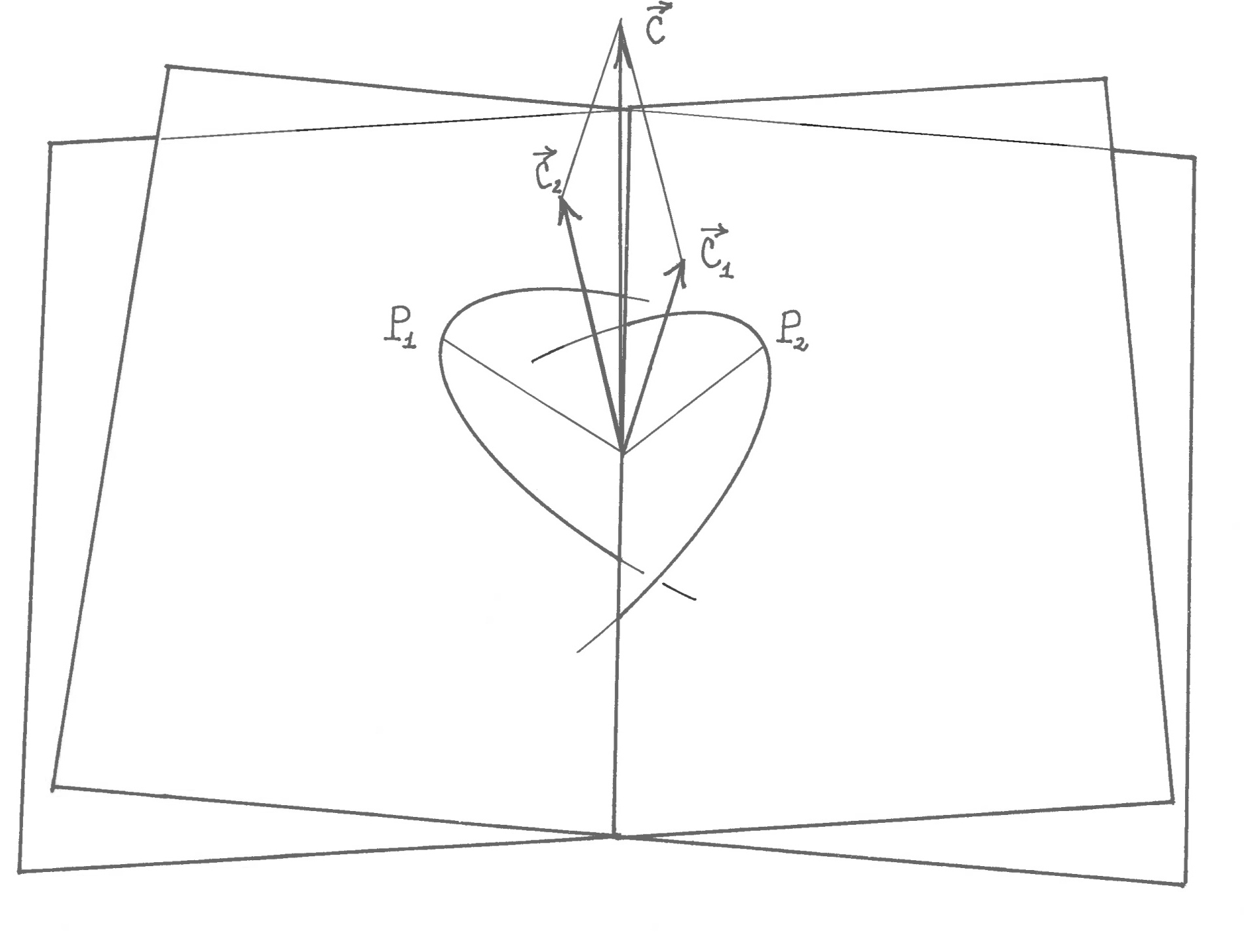
Figure 3: The construction underlying Jacobi reduction of the nodes.

$$Z_{1}=\frac{G}{2}+\frac{G_{1}^{2}-G_{2}^{2}}{2G}\ ,\quad Z_{2}=\frac{G}{2}-\frac{G_{1}^{2}-G_{2}^{2}}{2G}$$ (49)

where ${G}:=|{\mathbf{C}}|=\sqrt{{C}_{1}^{2}+{C}_{2}^{2}+{C}_{3}^{2}}$ is the Euclidean norm of ${\mathbf{C}}$. As $\mathbf{i}$ moves, the following fact is not obvious at all – in fact proved by R. Radau.

Theorem 1.4 (R. Radau, 1868, [16])

Replacing relations (48)–(49) inside the Hamiltonian (1) with $n=2$ written in Delaunay coordinates, one obtains a function, depending on $(\Lambda_{j},\ell_{j},G_{j},g_{j})$ ($j=1$, $2$) and $G$, whose Hamilton equations relatively to $(\Lambda_{j},\ell_{j},G_{j},g_{j})$ generate the motions of the coordinates $(\Lambda_{j},\ell_{j},G_{j},g_{j})$ referred to the rotating frame under the action of the Hamiltonian (1) with $n=2$. The motion of $Z_{j}$ and $\zeta_{j}$ can be recovered via (48)–(49).

1.4 Deprit coordinates

Arnold commented on the general problem of rotational degeneracy as follows:[1, Chap.III, §5, n. 5] In the case of more than three bodies [$n>2$] there is no such [analogue to Jacobi reduction of the nodes] elegant method of reducing the number of degrees of freedom […].

However, exactly 20 years later, in 1983, A. Deprit [7] discovered a set of canonical coordinates which, after a simple transformation, do the desired job and reduce to Jacobi’s when $n=2$. Let us describe them.
Consider the “partial angular momenta”

$${\mathbf{S}}_{j}({\mathbf{y}},{\mathbf{x}}):=\sum_{i=1}^{j}{\mathbf{C}}_{j}\ ;$$ (50)

with $\mathbf{C}_{i}$ as in (7). Notice that ${\mathbf{S}}_{n}={\mathbf{C}}$ is the total angular momentum of the system. Define the “Deprit nodes”

$$\left\{\begin{array}[]{l}\bm{{\nu}}_{i+1}:={\mathbf{S}}_{i+1}\times{\mathbf{C}}_{i+1}\ ,\qquad\ \ 1\leq i\leq n-1\\ \bm{{\nu}}_{1}:={\mathbf{S}}_{2}\times{\mathbf{C}}_{1}=-\bm{{\nu}}_{2}\\ \bm{{\nu}}_{n+1}:={\mathbf{k}}\times{\mathbf{C}}=:\bar{\bm{{\nu}}}\ .\end{array}\right.$$ (54)

If $n\geq 2$, Deprit’s coordinates

$${\cal D}_{ep}=(\mathbf{R},\mathbf{G},\bm{\Psi},\mathbf{r},\bm{\varphi},\bm{\psi})$$ (55)

with

$$\mathbf{R}=(R_{1},\ldots,R_{n})\,,\ \bm{\Psi}=(\Psi_{1},\ldots,\Psi_{n})\,,\ \mathbf{G}=(G_{1},\ldots,G_{n})\,,$$

$$\mathbf{r}=(r_{1},\ldots,r_{n})\,,\ \ \ \ \bm{\psi}=(\psi_{1},\ldots,\psi_{n})\,,\ \ \bm{\varphi}=(\varphi_{1},\ldots,\varphi_{n})\,.$$ (56)

are defined as follows (compare also Figures 6, 6 and 6):

$$\left\{\begin{array}[]{l}\displaystyle R_{i}:={\mathbf{y}}_{i}\cdot\frac{{\mathbf{x}}_{i}}{|{\mathbf{x}}_{i}|}\\ \\ \displaystyle r_{i}:=|{\mathbf{x}}_{i}|\end{array}\right.\qquad\left\{\begin{array}[]{l}\displaystyle G_{i}:=|{\mathbf{C}}_{i}|\\ \\ \displaystyle\varphi_{i}:={\alpha}_{{\mathbf{C}}_{i}}(\bm{{\nu}}_{i},{\mathbf{x}}_{i})\end{array}\right.$$ (63)

(64)

$$\Psi_{i}:=\left\{\begin{array}[]{l}\displaystyle|\mathbf{S}_{i+1}|\phantom{AAAAAAAA}\ 1\leq i\leq n-2\ (n\geq 3)\\ \\ \displaystyle C:=|\mathbf{C}|\phantom{AAAAAA}\ \ i=n-1\\ \\ \displaystyle Z:={\mathbf{C}}\cdot\mathbf{k}\phantom{AAAA.}\ \ \ i=n\end{array}\right.$$ (70)

$$\psi_{i}:=\left\{\begin{array}[]{l}\displaystyle{\alpha}_{{\mathbf{S}}_{i+1}}(\bm{{\nu}}_{i+2},\bm{{\nu}}_{i+1})\phantom{AAAa}1\leq i\leq n-2\ (n\geq 3)\\ \\ \gamma:={\alpha}_{\mathbf{C}}(\bar{\bm{{\nu}}},\bm{{\nu}}_{n})\phantom{AAAAA}i=n-1\\ \\ \displaystyle\zeta:={\alpha}_{\mathbf{k}}(\mathbf{i},\bar{\bm{{\nu}}})\phantom{AAAAAA}\ i=n\end{array}\right.$$ (76)

Figure 4: Deprit coordinates $Z$, $C$ and $\zeta$ fix the angular momentum in the initial reference frame $({\mathbf{i}},{\mathbf{j}},{\mathbf{k}})$.

Figure 5: The frames ${\rm D}_{i+1}$ and the coordinates $\Psi_{i}$, $\Psi_{i-1}$, $G_{i+1}$ and $\psi_{i}$.

Figure 6: The frames ${\rm H}_{i}$ and the coordinates $g_{i}$, $G_{i}$, $\ell_{i}$.

We have

Theorem 1.5 (A. Deprit, 1983, [7])

$\sum_{i=1}^{n}{\mathbf{y}}_{i}\cdot d{\mathbf{x}}_{i}={\mathbf{R}}\cdot d\mathbf{r}+\mathbf{\Psi}\cdot d\bm{\psi}+\mathbf{G}\cdot d\bm{\varphi}$ for all $n\in{{N}}$.

For later need, we formulate an equivalen statement of Theorem 1.5. We consider the coordinates

$${\cal D}_{e\ell}:=(\mathbf{Z},\mathbf{G},\mathbf{R},\bm{\zeta},\bm{\phi},\mathbf{r})$$ (77)

with

$$\mathbf{Z}=(Z_{1},\ldots,Z_{n})\,,\ \mathbf{G}=(G_{1},\ldots,G_{n})\,,\ \mathbf{R}=(R_{1},\ldots,R_{n})$$ (78)

$$\bm{\zeta}=(\zeta_{1},\ldots,\zeta_{n})\,,\ \ \ \bm{\phi}=(\phi_{1},\ldots,\phi_{n})\,,\ \mathbf{r}=(r_{1},\ldots,r_{n})$$

where $Z_{i}$, $G_{i}$, $\zeta_{i}$, are as in (15), $R_{i}$, $r_{i}$ are as in (63), and, finally,

$$\phi_{i}:={\alpha}_{\mathbf{C}_{i}}({\mathbf{n}}_{i},\mathbf{x}_{i})\,.$$

Let

$${\cal R}_{1}(i)=\left(\begin{array}[]{cccc}1&0&0\\ 0&\cos i&-\sin i\\ 0&\sin i&\cos i\end{array}\right)\ ,\qquad{\cal R}_{3}(\theta)=\left(\begin{array}[]{ccc}\cos\theta&-\sin\theta&0\\ \sin\theta&\cos\theta&0\\ 0&0&1\end{array}\right)$$ (79)

and

$${\mathbf{x}}={\cal R}_{3}(\theta){\cal R}_{1}(i)\bar{{\mathbf{x}}}\ ,\quad{\mathbf{y}}={\cal R}_{3}(\theta){\cal R}_{1}(i)\bar{{\mathbf{y}}}\ ,\quad{\mathbf{C}}:={\mathbf{x}}\times{\mathbf{y}}\ ,\quad\bar{\mathbf{C}}:=\bar{{\mathbf{x}}}\times\bar{{\mathbf{y}}}\ ,\quad\mathbf{i}=\left(\begin{array}[]{ccc}1\\ 0\\ 0\end{array}\right)\ ,\quad\mathbf{k}=\left(\begin{array}[]{ccc}0\\ 0\\ 1\end{array}\right)$$

with ${\mathbf{x}},\bar{{\mathbf{x}}},{\mathbf{y}},\bar{{\mathbf{y}}}\in^{3}$. The proof of the following fact is left to the reader.

Lemma 1.1

${\mathbf{y}}\cdot d{\mathbf{x}}={\mathbf{C}}\cdot\mathbf{k}d\theta+\bar{\mathbf{C}}\cdot\mathbf{i}di+\bar{{\mathbf{y}}}\cdot d\bar{{\mathbf{x}}}$.

Lemma 1.1 immediately implies

Lemma 1.2

$\mathbf{y}_{j}\cdot d\mathbf{x}_{j}=Z_{j}d\zeta_{j}+G_{j}d\phi_{j}+R_{j}dr_{j}\quad\forall\ j=1\,,\ldots\,,n\,,\ \forall n\in{{N}}$.

Indeed, we have

$$\left\{\begin{array}[]{lll}\mathbf{x}_{j}={\cal R}_{3}(\zeta_{j}){\cal R}_{1}(i^{*}_{j}){\mathbf{x}}_{j}^{*}\\ \mathbf{y}_{j}={\cal R}_{3}(\zeta_{j}){\cal R}_{1}(i^{*}_{j}){\mathbf{y}}_{j}^{*}\end{array}\right.\quad j=1\,,\ldots\,,\ n$$

where $i^{*}_{j}$ is the convex angle formed by $\mathbf{k}$ and $\mathbf{C}_{j}$ and, finally,

$${\mathbf{x}}_{j}^{*}=\left(\begin{array}[]{ccc}r_{j}\cos\phi_{j}\\ r_{j}\sin\phi_{j}\\ 0\end{array}\right)\,,\quad{\mathbf{y}}_{j}^{*}=\left(\begin{array}[]{ccc}R_{j}\cos\varphi_{j}-\frac{G_{j}}{r_{j}}\sin\phi_{j}\\ R_{j}\sin\varphi_{j}+\frac{G_{j}}{r_{j}}\cos\phi_{j}\\ 0\end{array}\right)$$ (86)

verify, as well known,

$${\mathbf{y}}_{j}^{*}\cdot d{\mathbf{x}}_{j}^{*}=R_{j}dr_{j}+G_{j}d\phi_{j}\,.$$ (87)

Then, by Lemma 1.1, (87) and as ${\mathbf{C}_{j}}^{*}\cdot\mathbf{i}=0$, we have

$$\mathbf{y}_{j}\cdot d\mathbf{x}_{j} = {\mathbf{C}}_{j}\cdot\mathbf{k}d\zeta_{j}+{\mathbf{C}_{j}}^{*}\cdot\mathbf{i}di_{j}+{\mathbf{y}}_{j}^{*}\cdot d{\mathbf{x}}_{j}^{*}$$

$$= Z_{j}d\zeta_{j}+G_{j}d\phi_{j}+R_{j}dr_{j}\,.\qquad\square$$

We denote as

$$\phi_{{\cal D}_{e\ell}}^{{\cal D}_{ep}}:\quad{\cal D}_{e\ell}=(\mathbf{Z},\mathbf{G},\mathbf{R},\bm{\zeta},\bm{\phi},\mathbf{r})\to{\cal D}_{ep}=(\bm{\Psi},\mathbf{G},\mathbf{R},\bm{\psi},\bm{\varphi},\mathbf{r})$$

the map which relates ${\cal D}_{e\ell}$ and ${\cal D}_{ep}$ and as

$$\mathaccent 866{\phi}_{{\cal D}_{e\ell}}^{{\cal D}_{ep}}:\quad\mathaccent 866{\cal D}_{e\ell}=(\mathbf{Z},\mathbf{G},\bm{\zeta},\bm{\phi})\to\mathaccent 866{\cal D}_{ep}=(\bm{\Psi},\mathbf{G},\bm{\psi},\bm{\varphi})$$

is the natural projections on the coordinates above. It is easy to check that $\mathaccent 866{\phi}_{{\cal D}_{e\ell}}^{{\cal D}_{ep}}$ is independent of $\mathbf{R}$ and $\mathbf{r}$. Indeed, $\mathaccent 866{\phi}_{{\cal D}_{e\ell}}^{{\cal D}_{ep}}$ has the expression

$$G_{j} = G_{j}\ ,$$

$$\varphi_{j} = \phi_{j}+{\alpha}_{{\mathbf{C}}_{i}}(\bm{{\nu}}_{j},\bar{\bm{{\nu}}}_{j})\ {\rm with}\ \bar{\bm{{\nu}}}_{j}={\mathbf{k}}\times{\mathbf{C}}_{j},$$

$$\Psi_{j} = \left\{\begin{array}[]{lll}|\mathbf{S}_{j+1}|&j\neq n\\ Z_{1}+\ldots+Z_{n}&j=n\end{array}\right.\quad$$ (90)

$$\psi_{j} = \left\{\begin{array}[]{lll}{\alpha}_{\mathbf{S}_{j+1}}(\bm{{\nu}}_{j+2},\bm{{\nu}}_{j+1})&j\neq n\\ {\alpha}_{\mathbf{k}}(\mathbf{i},\bar{\bm{\nu}})&j=n\end{array}\right.$$ (93)

where ${\mathbf{S}_{j+1}}$, $\bm{{\nu}}_{j}$, $\overline{\bm{{\nu}}}_{j}$ at the right hand sides are to be written as functions of ${\cal D}_{e\ell}$ (see (54) and (15)):

$$\left\{\begin{array}[]{lll}\displaystyle{{\mathbf{S}_{j+1}}=\sum_{i=1}^{j+1}G_{i}{\cal R}_{3}(\zeta_{i}){\cal R}_{1}(i^{{\cal D}el}_{i}){\mathbf{k}}}\\ \\ \displaystyle{\bm{{\nu}}_{j+1}=\left(\sum_{i=1}^{j+1}G_{i}{\cal R}_{3}(\zeta_{i}){\cal R}_{1}(i^{{\cal D}el}_{i}){\mathbf{k}}\right)\times G_{j+1}{\cal R}_{3}(\zeta_{j+1}){\cal R}_{1}(i^{{\cal D}el}_{j+1}){\mathbf{k}}\ ,\qquad\ \ 1\leq j\leq n-1}\\ \\ \displaystyle{\bm{{\nu}}_{1}=-\bm{{\nu}}_{2}=\left(\sum_{i=1}^{j+1}G_{i}{\cal R}_{3}(\zeta_{i}){\cal R}_{1}(i^{{\cal D}el}_{i}){\mathbf{k}}\right)\times G_{1}{\cal R}_{3}(\zeta_{1}){\cal R}_{1}(i^{{\cal D}el}_{1}){\mathbf{k}}}\\ \\ \displaystyle{\bm{{\nu}}_{n+1}=\bar{\bm{{\nu}}}{\mathbf{k}}\times\left(\sum_{i=1}^{n}G_{i}{\cal R}_{3}(\zeta_{i}){\cal R}_{1}(i^{{\cal D}el}_{i}){\mathbf{k}}\right)}\ .\end{array}\right.$$

with $i_{i}^{{\cal D}el}=\cos^{-1}\frac{G_{i}}{Z_{i}}$. As the right hand sides are defined only in terms of $\mathbf{C}_{j}$, so they are functions of $\mathbf{Z}$, $\bm{\zeta}$ and $\mathbf{G}$, while are independent of $\mathbf{R}$ and $\mathbf{r}$.

Theorem 1.6

Theorem 1.5 is equivalent to stress that

$$\ \mathaccent 866{\phi}_{{\cal D}_{e\ell}}^{{\cal D}_{ep}}\ verifies:\quad\mathbf{Z}\cdot d\bm{\zeta}+\mathbf{G}\cdot d\bm{\phi}=\mathbf{\Psi}\cdot d\bm{\psi}+\mathbf{G}\cdot d\bm{\varphi}\ \ for\ all\ n\in{{N}}\,.$$ (94)

Proof Use Lemma 1.2 and that the coordinates $(\mathbf{R},\mathbf{r})$ are shared by ${\cal D}_{ep}$ and ${\cal D}_{e\ell}$. $\quad\square$

We prove Theorem 1.5 ($\Longleftrightarrow$ (94)) by induction on $n$, with $n\geq 2$, as in [11].

Base step We prove the statement 1.5 with $n=2$. We first observe that, in such case, $({\mathbf{y}}_{j},{\mathbf{x}}_{j})$ are expressed, through $(\mathbf{R},\bm{\Psi},\mathbf{G},\mathbf{r},\bm{\psi},\bm{\varphi})$ via the formulae

$$\left\{\begin{array}[]{lll}\mathbf{x}_{j}={\cal R}_{3}(\zeta){\cal R}_{1}(i){\cal R}_{3}(\gamma){\cal R}_{1}(i_{j}){\mathbf{x}_{j}}_{\rm pl}\\ \mathbf{y}_{j}={\cal R}_{3}(\zeta){\cal R}_{1}(i){\cal R}_{3}(\gamma){\cal R}_{1}(i_{j}){\mathbf{y}_{j}}_{\rm pl}\end{array}\right.\quad j=1\,,\ 2$$

where $i$ is the convex angle formed by $\mathbf{k}$ and $\mathbf{C}$; $i_{j}$ is the convex angle formed by $\mathbf{C}$ and $\mathbf{C}_{j}$ and, finally, ${\mathbf{x}_{j}}_{\rm pl}$, ${\mathbf{y}_{j}}_{\rm pl}$ are as in (86), with $\phi_{j}$ replaced by $\varphi_{j}$.
Using Lemma 1.1 twice, one easily finds

$${\mathbf{y}}_{j}\cdot d{{\mathbf{x}}}_{j}= {{\mathbf{C}}_{j}}\cdot{\mathbf{k}}\,d\zeta+{\bar{\mathbf{C}}_{j}}\cdot{\mathbf{i}}\,di+{\bar{\mathbf{C}}_{j}}\cdot{\mathbf{k}}\,d\gamma+\ {{\mathbf{C}}_{j}}_{\rm pl}\cdot{\mathbf{i}}\,d(i_{j})$$

$$+{{\mathbf{y}}_{j}}_{\rm pl}\cdot d{{{\mathbf{x}}}_{j}}_{\rm pl}$$

$$= {{\mathbf{C}}_{j}}\cdot{\mathbf{k}}\,d\zeta+{{\mathbf{C}}_{j}}\cdot{\mathbf{e}}_{1}\,di+{{\mathbf{C}}_{j}}\cdot{\mathbf{e}}_{3}\,d\gamma+{{\mathbf{y}}_{j}}_{\rm pl}\cdot d{{{\mathbf{x}}}_{j}}_{\rm pl}$$ (95)

We have used ${{\mathbf{C}}_{j}}_{\rm pl}\cdot{\mathbf{i}}=0$, ${{\mathbf{C}}_{j}}={\cal R}_{3}(\zeta){\cal R}_{1}(i){\bar{\mathbf{C}}_{j}}$ and we have let

$$\mathbf{e}_{1}:={\cal R}_{3}(\zeta){\cal R}_{1}(i)\mathbf{i}\,,\qquad\mathbf{e}_{3}:={\cal R}_{3}(\zeta){\cal R}_{1}(i)\mathbf{k}\ .$$ (96)

Taking the sum of (1.4) with $j=1$, $2$ and using (87) and recognizing that

$$\left\{\begin{array}[]{l}({{\mathbf{C}}_{1}}+{\mathbf{C}}_{2})\cdot{\mathbf{k}}={\mathbf{C}}\cdot{\mathbf{k}}=Z\\ ({{\mathbf{C}}_{1}}+{\mathbf{C}}_{2})\cdot{\mathbf{e}}_{1}={\mathbf{C}}\cdot{\mathbf{e}}_{1}=0\\ ({{\mathbf{C}}_{1}}+{\mathbf{C}}_{2})\cdot{\mathbf{e}}_{3}={\mathbf{C}}\cdot{\mathbf{e}}_{3}=C\end{array}\right.$$

we have the proof.       

Induction The inductive step is made on the statement (94). The map $\mathaccent 866{\phi}_{{\cal D}_{e\ell}}^{{\cal D}_{ep}}$ in (94) will be named $\mathaccent 866{\phi}_{n}$. We assume that (94) holds for a given $n\geq 2$ and prove it for $n+1$. Consider the map

$$\phi^{*}_{n+1}:\quad\mathaccent 866{\cal D}_{e\ell,n+1}=(\mathbf{Z},\mathbf{G},\bm{\zeta},\bm{\phi})\to\mathaccent 869{\cal D}_{ep,n+1}=(\bm{\Psi}^{*},\mathbf{G}^{*},\bm{\psi}^{*},\bm{\varphi}^{*})$$

defined as follows. If

$$\mathbf{Z}=\big{(}\mathaccent 869{\mathbf{Z}},Z_{n+1}\big{)}\,,\ \mathbf{G}=\big{(}\mathaccent 869{\mathbf{G}},G_{n+1}\big{)}\,,\ \bm{\zeta}=\big{(}\mathaccent 869{\bm{\zeta}},\zeta_{n+1}\big{)}\,,\ \bm{\phi}=\big{(}\mathaccent 869{\bm{\phi}},\phi_{n+1}\big{)}$$

where the tilded arguments have dimension $n$, we let

$$(\mathaccent 869{\bm{\Psi}},\mathaccent 869{\mathbf{G}},\mathaccent 869{\bm{\psi}},\mathaccent 869{\bm{\varphi}})=\phi_{n}(\mathaccent 869{\mathbf{Z}},\mathaccent 869{\mathbf{G}},\mathaccent 869{\bm{\zeta}},\mathaccent 869{\bm{\phi}})$$

and then

$$\phi^{*}_{n+1}(\mathbf{Z},\mathbf{G},\bm{\zeta},\bm{\phi}):=\big{(}(\mathaccent 869{\bm{\Psi}},Z_{n+1}),(\mathaccent 869{\mathbf{G}},G_{n+1}),(\mathaccent 869{\bm{\psi}},\zeta_{n+1}),(\mathaccent 869{\bm{\varphi}},\phi_{n+1})\big{)}=:(\bm{\Psi}^{*},\mathbf{G}^{*},\bm{\psi}^{*},\bm{\varphi}^{*})$$

By the inductive assumption, $\phi_{n}$ verifies

$$\mathaccent 869{\mathbf{Z}}\cdot d\mathaccent 869{\bm{\zeta}}+\mathaccent 869{\mathbf{G}}\cdot d\mathaccent 869{\bm{\phi}}=\mathaccent 869{\mathbf{\Psi}}\cdot d\mathaccent 869{\bm{\psi}}+\mathaccent 869{\mathbf{G}}\cdot d\mathaccent 869{\bm{\varphi}}$$

and hence $\phi^{*}_{n+1}$ verifies

$${\mathbf{Z}}\cdot d{\bm{\zeta}}+{\mathbf{G}}\cdot d{\bm{\phi}} = {\mathbf{\Psi}}^{*}\cdot d{\bm{\psi}}^{*}+{\mathbf{G}}^{*}\cdot d{\bm{\varphi}}^{*}$$ (97)

$$= \mathaccent 869{\mathbf{\Psi}}\cdot d\mathaccent 869{\bm{\psi}}+\mathaccent 869{\mathbf{G}}\cdot d\mathaccent 869{\bm{\varphi}}+Z_{n+1}d\zeta_{n+1}+G_{n+1}d\phi_{n+1}$$

$$= \left(\sum_{j=1}^{n-2}\mathaccent 869{\Psi}_{j}\cdot d\mathaccent 869{\psi}_{j}+\mathaccent 869{\mathbf{G}}\cdot d\mathaccent 869{\bm{\varphi}}\right)+\mathaccent 869{\Psi}_{n-1}\cdot d\mathaccent 869{\psi}_{n-1}+\mathaccent 869{\Psi}_{n}\cdot d\mathaccent 869{\psi}_{n}$$

$$+ Z_{n+1}d\zeta_{n+1}+G_{n+1}d\phi_{n+1}\quad{\rm split\ the\ rhs}$$

having split

$$\mathaccent 869{\bm{\Psi}}=(\mathaccent 869{\Psi}_{1},\ldots,\mathaccent 869{\Psi}_{n})\,,\ \mathaccent 869{\bm{\psi}}=(\mathaccent 869{\psi}_{1},\ldots,\mathaccent 869{\psi}_{n})\,.$$

We moreover define a map $\phi_{*,n+1}$ on $(\bm{\Psi}^{*},\mathbf{G}^{*},\bm{\psi}^{*},\bm{\varphi}^{*})$ acting as

$$(\bm{\Psi}_{*},\mathbf{G}_{*},\bm{\psi}_{*},\bm{\varphi}_{*})=\phi_{2}\big{(}(\mathaccent 869{\Psi}_{n},Z_{n+1}),(\mathaccent 869{\Psi}_{n-1},G_{n+1}),(\mathaccent 869{\psi}_{n},\zeta_{n+1}),(\mathaccent 869{\psi}_{n-1},\phi_{n+1})\big{)}$$

on the designed variables, and as the identity on the remaining ones. Note that the arguments at left hand side have dimension $2$, that $\mathbf{G}_{*}=(\mathaccent 869{\Psi}_{n-1},G_{n+1})$, and put $\bm{\varphi}_{*}=(\varphi_{*,1},\varphi_{*,2})$. Again by the inductive assumption, we have

$$\mathaccent 869{\Psi}_{n-1}\cdot d\mathaccent 869{\psi}_{n-1}+\mathaccent 869{\Psi}_{n}\cdot d\mathaccent 869{\psi}_{n}+Z_{n+1}d\zeta_{n+1}+G_{n+1}d\phi_{n+1}={\mathbf{\Psi}}_{*}\cdot d{\bm{\psi}}_{*}+{\mathbf{G}}_{*}\cdot d{\bm{\varphi}}_{*}$$ (98)

Let us now look at the composition

$$\phi_{*,n+1}\circ\phi^{*}_{n+1}$$ (99)

It acts as

$$(\mathbf{Z},\mathbf{G},\bm{\zeta},\bm{\phi}) \to \big{(}(\mathaccent 869{\Psi}_{1},\ldots,\mathaccent 869{\Psi}_{n-2},\mathaccent 869{\Psi}_{n-1},\bm{\Psi}_{*}),(\mathaccent 869{\mathbf{G}},G_{n+1}),(\mathaccent 869{\psi}_{1},\ldots,\mathaccent 869{\psi}_{n-2},{\varphi}_{*1},\bm{\psi}_{*}),(\mathaccent 869{\bm{\varphi}},{\varphi}_{*2})$$

$$=:(\bm{\Psi},\mathbf{G},\bm{\psi},\bm{\varphi})\big{)}$$

and, by (97) and (98), verifies

$${\mathbf{Z}}\cdot d{\bm{\zeta}}+{\mathbf{G}}\cdot d{\bm{\phi}} = \left(\sum_{j=1}^{n-2}\mathaccent 869{\Psi}_{j}\cdot d\mathaccent 869{\psi}_{j}+\mathaccent 869{\mathbf{G}}\cdot d\mathaccent 869{\bm{\varphi}}\right)+{\mathbf{\Psi}}_{*}\cdot d{\bm{\psi}}_{*}+{\mathbf{G}}_{*}\cdot d{\bm{\varphi}}_{*}$$

$$= {\mathbf{\Psi}}\cdot d{\bm{\psi}}+{\mathbf{G}}\cdot d{\bm{\varphi}}\,.$$

It is not difficult to recognize – using (1.4) – that the map (99) coincides with $\phi_{n+1}$. For the details, we refer to [11, 3]. $\quad\square$

The Deprit map

In this section, we provide the explicit expression of the map

$$\phi_{{\cal C}}^{{\cal D}_{ep}}:\quad{\cal C}=(\mathbf{y}_{1},\ldots,\mathbf{y}_{n},\mathbf{x}_{1},\ldots,\mathbf{x}_{n})\to{\cal D}_{ep}=(\bm{\Psi},\mathbf{G},\mathbf{R},\bm{\psi},\bm{\varphi},\mathbf{r})\,.$$ (100)

The discussion in the previous section shows that each orbital frame ${\cal H}_{i}$, $i=1$, $\ldots$, $n$, can be reached via a sequence of transformations which overlap the ${\rm D}_{n+1}:=({\mathbf{i}},{\mathbf{j}},{\mathbf{k}})$ to ${\cal H}_{i}$ through the following diagram (named tree by Deprit):

$$\begin{array}[]{cccccccccccccccccc}\displaystyle{\rm D}_{n+1}&\to&{\rm D}_{n}&\to&{\rm D}_{n-1}&\to&\cdots&\to&{\rm D}_{2}&\to{\rm H}_{1}\\ \\ \displaystyle\hfil&&\downarrow&&\downarrow&&\vdots&&\downarrow&&\\ \\ \displaystyle\hfil&&{\rm H}_{n}&&{\rm H}_{n-1}&&\vdots&&{\rm H}_{2}&&&\\ \\ \end{array}$$

In turn,

• the transition ${\rm D}_{n+1}\to\rm D_{n}$ is described by the sequence of rotations ${\cal R}_{3}(\psi_{n}){\cal R}_{1}(i_{n})$, with $\cos i_{n}=\frac{Z}{\rm G}=\frac{\Psi_{n}}{\Psi_{n-1}}$ (see figure 6);

• the transitions ${\rm D}_{i+1}\to\rm H_{i+1}$, $i+1=n-1$, $\ldots$, $2$, are described by the sequence of rotations ${\cal R}_{3}(\psi_{i}){\cal R}_{1}(i_{i})$, with $\cos i_{i}=\frac{\Psi_{i}^{2}+G_{i}^{2}-\Psi_{i-1}^{2}}{2\Psi_{i}G_{i+1}}$ (see figure 6);

• the transitions ${\rm D}_{i+1}\to{\rm D}_{i}$, $i+1=n-1$, $\ldots$, $1$, are related by the sequence of rotations ${\cal R}_{3}(\psi_{i}+\pi){\cal R}_{1}(i^{*}_{i}):={\cal R}_{3}(\psi_{i}^{*}){\cal R}_{1}(i^{*}_{i})$, with $\cos i^{*}_{i}=\frac{\Psi_{i}^{2}-G_{i+1}^{2}+\Psi_{i-1}^{2}}{2\Psi_{i-1}\Psi_{i}}$ (see figure 6, noticing that $\mathbf{S}_{i+1}\times\mathbf{C}_{i+1}=-\mathbf{S}_{i+1}\times\mathbf{S}_{i}$).

Then we find that (100) has the expression

$$\left\{\begin{array}[]{lll}\displaystyle{\mathbf{y}}_{i}={\cal R}_{i}^{n}{\mathbf{y}}^{*}_{i}\\ \\ \displaystyle{\mathbf{x}}_{i}={\cal R}_{i}^{n}{\mathbf{x}}^{*}_{i}\end{array}\right.$$

with

$${\cal R}_{i}^{n}:={\cal R}_{3}(\psi_{n}){\cal R}_{1}(i_{n}){\cal R}_{3}(\psi^{*}_{n-1}){\cal R}_{1}(i^{*}_{n-1})\cdots{\cal R}_{3}(\psi^{*}_{i}){\cal R}_{1}(i^{*}_{i}){\cal R}_{3}(\psi_{i-1}){\cal R}_{1}(i_{i-1})$$

and ${\mathbf{y}}^{*}_{i}$, ${\mathbf{x}}^{*}_{i}$ as in (86).

1.5 The map ${\cal K}$

Figure 7: The reference frames $\hat{\rm F}_{j}$ and the ${\cal K}$–coordinates $\hat{\kappa}_{j-1}$, $r_{j}$, $R_{j}$ $j=2$, $\ldots$, $n$.

Figure 8: The reference $\hat{\rm F}_{1}$ and the ${\cal K}$–coordinates $\hat{\Theta}_{1}$, $\hat{\vartheta}_{1}$.

Figure 9: The reference frames $\hat{\rm G}_{j}$ and the ${\cal K}$–coordinates $\hat{\vartheta}_{j}$, $\hat{\Theta}_{j}$, $\hat{\chi}_{j-1}$, $j=1$, $\ldots$, $n$. When $j=2$, take $\hat{\chi}_{0}:=\hat{\Theta}_{1}$; when $j=1$, disregard ${\mathbf{S}}_{0}$, $\hat{\bm{\nu}}_{0}$ and $\hat{\chi}_{-1}$.

The ${\cal K}$–coordinates have been described in [12] for $n=2$ and generalized to any $n\in{{N}}$, $n\geq 2$ in [14]. Here, for sake of uniformity with the coordinates ${\cal D}_{ep}$, we change notations a little bit compared to [14]. We let

$${\cal K}=(\hat{\bm{\Theta}},\hat{\bm{\chi}},{\mathbf{R}},\hat{\bm{\vartheta}},\hat{\bm{{\kappa}}},{\mathbf{r}})$$

where $\mathbf{R}$, $\mathbf{r}$ are as in (63), while

$$\begin{array}[]{lll}\displaystyle\hat{\bm{\Theta}}=(\hat{\Theta}_{1},\ldots,\hat{\Theta}_{n}),&\hat{\bm{\vartheta}}=(\hat{\vartheta}_{1},\ldots,\hat{\vartheta}_{n})\\ \\ \displaystyle\hat{\bm{\chi}}=(\hat{\chi}_{1},\ldots,\hat{\chi}_{n}),&\hat{\bm{{\kappa}}}=(\hat{\kappa}_{1},\ldots,\hat{\kappa}_{n})\end{array}$$

are defined as follows. Let $\mathbf{S}_{j}$ be as in (50). Define the ${\cal K}$-nodes

$$\hat{\bm{{\nu}}}_{j}:=\left\{\begin{array}[]{llll}\displaystyle{\mathbf{k}}\times{\mathbf{C}}&j=n\\ \\ \displaystyle{\mathbf{x}}_{j+1}\times{\mathbf{S}}_{j}&j=1,\ldots,n-1\end{array}\right.\qquad\hat{\mathbf{n}}_{j}:=\displaystyle{\mathbf{S}}_{j}\times{\mathbf{x}}_{j}\qquad j=1,\ldots,n.$$ (103)

and then the ${\cal K}$coordinates as follows.

$$\begin{array}[]{llllrrr}\displaystyle\hat{\Theta}_{j}:=\left\{\begin{array}[]{lrrr}\displaystyle{\mathbf{S}}_{j}\cdot\frac{{\mathbf{x}}_{j}}{|{\mathbf{x}}_{j}|}\\ \\ \displaystyle|{\mathbf{C}}_{1}|\end{array}\right.&\hat{\vartheta}_{j}:=\left\{\begin{array}[]{lrrr}\displaystyle{\alpha}_{{\mathbf{x}}_{j}}(\hat{\mathbf{n}}_{j},\hat{\bm{\nu}}_{j-1})&2\leq j\leq n\\ \\ \displaystyle{\alpha}_{{\mathbf{C}}_{1}}(\hat{\bm{\nu}}_{1},\hat{\mathbf{n}}_{1})&j=1\end{array}\right.\\ \\ \displaystyle\hat{\chi}_{j}:=\left\{\begin{array}[]{lrrr}Z:={\mathbf{C}}\cdot{\mathbf{k}}\\ \\ C:=|{\mathbf{C}}|\\ \\ |{\mathbf{S}}_{j+1}|\end{array}\right.&\hat{{\kappa}}_{j}:=\left\{\begin{array}[]{lrrr}\zeta:={\alpha}_{{\mathbf{k}}}({\mathbf{i}},\hat{\bm{{\nu}}}_{n})&j=n\\ \\ \gamma:={\alpha}_{{\mathbf{S}}_{n}}(\hat{\bm{{\nu}}}_{n},\hat{\mathbf{n}}_{n})&j=n-1\\ \\ {\alpha}_{{\mathbf{S}}_{j+1}}(\hat{\bm{{\nu}}}_{j+1},\hat{\mathbf{n}}_{j+1})&1\leq j\leq n-2\ (n\geq 3)\par\end{array}\right.\end{array}$$ (123)

Remark 1.2

Note that the node $\hat{\bm{{\nu}}}_{n}$ coincides with $\overline{\bm{{\nu}}}={\bm{{\nu}}}_{n+1}$ in (54); the coordinates $Z$ and $\zeta$ are the same as in (63) and, finally, the coordinates $\bm{\chi}$ coincide with the coordinates $\hat{\bm{\Psi}}$ in (63). In particular, ${\cal D}_{ep}$ and ${\cal K}$ share the construction in Figure 6. The geometrical meaning of the other ${\cal K}$–coordinates is pointed out in the next section.

A chain of reference frames

We consider the following chain of vectors

$$\begin{array}[]{cccccccccccccccccc}\displaystyle{\mathbf{k}}&\to&{\mathbf{S}}_{n}={\mathbf{C}}&\to&{\mathbf{x}}_{n}&\to&\cdots&\to&{\mathbf{S}}_{j}&\to&{\mathbf{x}}_{j}&\to&{\mathbf{S}}_{j-1}&\to&\cdots&\to&{\mathbf{S}}_{1}={\mathbf{C}}_{1}\\ \\ \displaystyle\hfil&&\Downarrow&&\Downarrow&&\vdots&&\Downarrow&&\Downarrow&&\Downarrow&&\vdots&&\Downarrow\\ \\ \displaystyle\hfil&&\hat{\bm{{\nu}}}_{n}&&\hat{\mathbf{n}}_{1}&&\vdots&&\hat{\bm{{\nu}}}_{j}&&\hat{\mathbf{n}}_{j}&&\hat{\bm{{\nu}}}_{j-1}&&\vdots&&\hat{\bm{{\nu}}}_{1}\\ \end{array}$$ (129)

where $\hat{\bm{{\nu}}}_{j}$, $\hat{\mathbf{n}}_{j}$ are the ${\cal K}$-nodes in (103), given by the skew-product of the two consecutive vectors in the chain.

We associate to this chain of vectors the following chain of frames

$$\begin{array}[]{cccccccccccccccccc}\displaystyle\hat{\rm G}_{n+1}&\to&\hat{\rm F}_{n}&\to&\hat{\rm G}_{n}&\to&\cdots&\to&\hat{\rm F}_{j}&\to&\hat{\rm G}_{j}&\to&\hat{\rm F}_{j-1}&\to&\cdots&\to&\hat{\rm G}_{1}\end{array}$$ (131)

where $\hat{\rm G}_{n+1}=({\mathbf{i}},{\mathbf{j}},{\mathbf{k}})$ is the initial prefixed frame and the frames, while $\hat{\rm F}_{j}$, $\hat{\rm G}_{j}$ are frames defined via

$$\hat{\rm F}_{j}=(\hat{\bm{{\nu}}}_{j},\ \cdot,{\mathbf{S}}_{j})\quad\hat{\rm G}_{j}=(\hat{\mathbf{n}}_{j},\ \cdot,{\mathbf{x}}_{j})\qquad j=1,\cdots,n.$$ (132)

By construction, each frame in the chain has its first axis coinciding with the intersection of horizontal plane with the horizontal plane of the previous frame (hence, in particular, $\hat{\bm{{\nu}}}_{j}\perp{\mathbf{S}}_{j}$ and $\hat{\mathbf{n}}_{j}\perp{\mathbf{x}}_{j}$).

Explicit expression of the ${\cal K}$–map

We now derive the explicit formulae of the map which relates the coordinates (123) to the coordinates $({\mathbf{y}}_{1},\ldots,{\mathbf{y}}_{n},{\mathbf{x}}_{1},\ldots,{\mathbf{x}}_{n})$. We shall prove that such map has the expression

$$\left\{\begin{array}[]{ll}\displaystyle{\mathbf{x}}_{j}={\mathbf{x}}^{n}_{j}:={\cal R}_{j}^{n}\tilde{\mathbf{x}}_{j}\\ \\ \displaystyle{\mathbf{y}}_{j}={\mathbf{y}}^{n}_{j}:={\cal R}_{j}^{n}\tilde{\mathbf{y}}_{j}\end{array}\right.$$ (136)

where

$$\left\{\begin{array}[]{lll}\displaystyle{\cal R}^{n}_{j}:=\hat{\cal T}_{n}\hat{\cal S}_{n}\cdots\hat{\cal T}_{j+1}\hat{\cal S}_{j+1}\hat{\cal T}_{j}\hat{\cal S}_{j}\\ \\ \displaystyle\tilde{\mathbf{x}}_{j}:=r_{j}{\mathbf{k}}\\ \\ \displaystyle\tilde{\mathbf{y}}_{j}:=R_{j}{\mathbf{k}}+\frac{1}{r_{j}}\tilde{\mathbf{C}}_{j}\times{\mathbf{k}}\\ \\ \displaystyle\tilde{\mathbf{C}}_{j}:=\left\{\begin{array}[]{ll}\displaystyle\hat{\cal S}^{-1}_{j}\Big{(}\hat{\chi}_{j-1}{\mathbf{k}}-\hat{\chi}_{j-2}\hat{\cal S}_{j}\hat{\cal T}_{j-1}{\mathbf{k}}\Big{)}=\tilde{\mathbf{x}}_{j}\times\tilde{\mathbf{y}}_{j}&i=2,\ldots,n\\ \\ \displaystyle\hat{\Theta}_{1}\hat{\cal S}^{-1}_{1}{\mathbf{k}}&j=1\end{array}\right.\end{array}\right.$$ (147)

where $\hat{\cal T}_{j}$, $\hat{\cal S}_{j}$ have the expressions

$$\hat{\cal T}_{j}:=\left\{\begin{array}[]{ll}{\cal R}_{3}(\zeta){\cal R}_{1}(\iota_{n})&j=n\\ \\ {\cal R}_{3}(\hat{\vartheta}_{j+1}){\cal R}_{1}(\iota_{j})&1\leq j\leq n-1\end{array}\right.\qquad\hat{\cal S}_{j}:=\left\{\begin{array}[]{lll}\displaystyle{\cal R}_{3}(\hat{\kappa}_{j-1}){\cal R}_{1}({\rm i}_{j}),&2\leq j\leq n\\ \\ \displaystyle{\cal R}_{3}(\hat{\vartheta}_{1}){\cal R}_{1}(\frac{{\pi}}{2}),&j=1\end{array}\right.$$ (154)

with

$$\left\{\begin{array}[]{lll}\displaystyle\cos\iota_{n}=\frac{Z}{\hat{\chi}_{n-1}}&\\ \\ \displaystyle\cos\iota_{j}=\frac{\hat{\Theta}_{j+1}}{\hat{\chi}_{j-1}}&2\leq j\leq n-1\ (n\geq 3)\\ \\ \displaystyle\cos\iota_{1}=\frac{\hat{\Theta}_{2}}{\hat{\Theta}_{1}}&\end{array}\right.$$ (160)

$$\left\{\begin{array}[]{lll}\displaystyle\cos{\rm i}_{j}:=\frac{\hat{\Theta}_{j}}{\hat{\chi}_{j-1}},\quad 2\leq j\leq n\\ \\ \displaystyle{\rm i}_{1}=\frac{{\pi}}{2}\end{array}\right.$$ (164)

Indeed, $\hat{\cal T}_{j}$ is the rotation matrix which describes the change of coordinates from $\hat{\rm G}_{j+1}$ to $\hat{\rm F}_{j}$, while $\hat{\cal S}_{j}$ describes the change of coordinates from $\hat{\rm F}_{j}$ to $\hat{\rm G}_{j}$, as it follows from the definitions of $(\hat{\Theta},\hat{\chi},\hat{\vartheta},\hat{\kappa})$ in (123) (see also Figures 9, 9 and 9). The formulae (136)–(160) are obtained considering the following sequence of transformations

$$\begin{array}[]{cccccccccccccccccc}&\hat{\cal T}_{n}&&\hat{\cal S}_{n}&&&\cdots&&&\hat{\cal S}_{j}&&\hat{\cal T}_{j-1}&&&\cdots&\hat{\cal S}_{1}&\\ \\ \displaystyle\hat{\rm G}_{n+1}&\to&\hat{\rm F}_{n}&\to&\hat{\rm G}_{n}&\to&\cdots&\to&\hat{\rm F}_{j}&\to&\hat{\rm G}_{j}&\to&\hat{\rm F}_{j-1}&\to&\cdots&\to&\hat{\rm G}_{1}\end{array}$$

connecting $\hat{\rm G}_{n}$ to any other frame in the chain. From this, and the definitions of the frames (132), one finds

$${\mathbf{S}}_{j}=\left\{\begin{array}[]{lll}\displaystyle\chi_{j-1}\hat{\cal T}_{n}\hat{\cal S}_{n}\cdots\hat{\cal T}_{j+1}\hat{\cal S}_{j+1}\hat{\cal T}_{j}{\mathbf{k}}&j=2\,\ldots\,n\\ \\ \hat{\Theta}_{1}\hat{\cal T}_{n}\hat{\cal S}_{n}\cdots\hat{\cal T}_{2}\hat{\cal S}_{2}{\cal T}_{1}{\mathbf{k}}&j=1\end{array}\right.\qquad{\mathbf{x}}_{j}=r_{j}\hat{\cal T}_{n}\hat{\cal S}_{n}\cdots\hat{\cal T}_{j+1}\hat{\cal S}_{j+1}\hat{\cal T}_{j}\hat{\cal S}_{j}{\mathbf{k}}$$

whence

$${\mathbf{C}}_{j}=\left\{\begin{array}[]{lll}\displaystyle{\mathbf{S}}_{j}-{\mathbf{S}}_{j-1}=\hat{\cal T}_{n}\hat{\cal S}_{n}\cdots\hat{\cal T}_{j+1}\hat{\cal S}_{j+1}\hat{\cal T}_{j}\Big{(}\hat{\chi}_{j-1}{\mathbf{k}}-\hat{\chi}_{j-2}\hat{\cal S}_{j}\hat{\cal T}_{j-1}{\mathbf{k}}\Big{)}&j=2\,,\ \ldots\,,n\\ \\ \displaystyle{\mathbf{S}}_{1}=\hat{\Theta}_{1}\hat{\cal T}_{n}\hat{\cal S}_{n}\cdots\hat{\cal T}_{2}\hat{\cal S}_{2}\hat{\cal T}_{1}{\mathbf{k}}&j=1\end{array}\right.$$

and finally

$${\mathbf{y}}_{j}=\frac{{R}_{j}}{{r}_{j}}{\mathbf{x}}_{j}+\frac{1}{r_{j}^{2}}{\mathbf{C}}_{j}\times{\mathbf{x}}_{j}$$

Collecting such formulae, one finds (136)–(160).

Canonical character of ${\cal K}$

Lemma 1.3

${\cal K}$ preserves the standard Liouville 1-form:

$$\sum_{j=1}^{n}{\mathbf{y}}_{j}\cdot d{\mathbf{x}}_{j}=\hat{\bm{\Theta}}\cdot d\hat{\bm{\vartheta}}+\hat{\bm{\chi}}\cdot d\hat{\bm{{\kappa}}}+{\mathbf{R}}\cdot d{\mathbf{r}}.$$ (166)

The proof of Lemma 1.3 again relies in Lemma 1.1.

Proof We use the expression in (136). We also define

$${\mathbf{C}}_{j}^{n}:={\cal R}_{j}^{n}\tilde{\mathbf{C}}_{j}\,,\qquad\overline{\mathbf{C}}^{n}_{j}:=\overline{\cal R}_{j}^{n}\tilde{\mathbf{C}}_{j}\,,\quad\overline{\cal R}_{j}^{n}:=\hat{\cal T}_{n}^{-1}{\cal R}_{j}^{n}$$

Applying Lemma 1.1 twice, we get

$${\mathbf{y}}^{n}_{j}\cdot d{\mathbf{x}}^{n}_{j}={\mathbf{C}}^{n}_{j}\cdot{\mathbf{k}}\,d\zeta+\overline{\mathbf{C}}^{n}_{j}\cdot{\mathbf{i}}\,d\iota_{n}+\overline{\mathbf{C}}^{n}_{j}\cdot{\mathbf{k}}\,d\hat{\kappa}_{n-1}+{\mathbf{C}}^{n-1}_{j}\cdot{\mathbf{i}}\,d{\rm i}_{n}+{\mathbf{y}}^{n-1}_{j}\cdot d{\mathbf{x}}^{n-1}_{j}\,.$$

Continuing in this way, after $n-j+1$ iterates we arrive at

$${\mathbf{y}}_{j}\cdot d{\mathbf{x}}_{j} = {\mathbf{C}}^{n}_{j}\cdot{\mathbf{k}}\,d\zeta+\overline{\mathbf{C}}^{n}_{j}\cdot{\mathbf{i}}\,d\iota_{n}+\overline{\mathbf{C}}^{n}_{j}\cdot{\mathbf{k}}\,d\hat{\kappa}_{n-1}+{\mathbf{C}}^{n-1}_{j}\cdot{\mathbf{i}}\,d{\rm i}_{n}$$ (167)

$$+ \sum_{k=j}^{n-1}\Big{(}{\mathbf{C}}^{k}_{j}\cdot{\mathbf{k}}\,d\hat{\vartheta}_{k+1}+\overline{\mathbf{C}}^{k}_{j}\cdot{\mathbf{i}}\,d\iota_{k}+\overline{\mathbf{C}}^{k}_{j}\cdot{\mathbf{k}}\,d\hat{\kappa}_{k-1}+{\mathbf{C}}^{k-1}_{j}\cdot{\mathbf{i}}\,d{\rm i}_{k}\Big{)}$$

$$+ \mathaccent 869{{\mathbf{y}}}_{j}\cdot d\mathaccent 869{{\mathbf{x}}}_{j}$$

with

$${\rm i}_{1}:=\frac{{\pi}}{2}\,,\ {\kappa}_{0}:=\hat{\vartheta}_{1}\,,\quad{\mathbf{C}}^{j-1}_{j}:=\tilde{\mathbf{C}}_{j}=\mathaccent 869{{\mathbf{x}}}_{j}\times\mathaccent 869{{\mathbf{y}}}_{j}\,.$$

We take the sum of (167) with $j=1$, $\ldots$, $n$. Exchanging the sums

$$\sum_{j=1}^{n}\sum_{k=j}^{n-1}=\sum_{k=1}^{n-1}\sum_{j=1}^{k}$$

and recognizing that

$$\left\{\begin{array}[]{lll}\displaystyle\sum_{j=1}^{k}{\mathbf{C}}^{k}_{j}=\left\{\begin{array}[]{lll}\hat{\cal S}_{k+1}^{-1}\hat{\cal T}_{k+1}^{-1}\cdots\hat{\cal S}_{n}^{-1}\hat{\cal T}_{n}^{-1}{\mathbf{S}}_{k}=\chi_{k-1}\hat{\cal T}_{k}{\mathbf{k}}&1\leq k\leq n-1\\ \\ \displaystyle{\mathbf{S}}_{n}=\chi_{n-1}\hat{\cal T}_{n}{\mathbf{k}}&k=n\end{array}\right.\\ \\ \displaystyle\sum_{j=1}^{k}{\mathbf{C}}^{k-1}_{j}=\left\{\begin{array}[]{lll}\hat{\cal S}_{k}^{-1}\hat{\cal T}_{k}^{-1}\cdots\hat{\cal S}_{n}^{-1}\hat{\cal T}_{n}^{-1}{\mathbf{S}}_{k}=\chi_{k-1}\hat{\cal S}_{k}^{-1}{\mathbf{k}}&1\leq k\leq n-1\\ \\ \displaystyle\hat{\cal S}_{n}^{-1}\hat{\cal T}_{n}^{-1}{\mathbf{S}}_{n}=\chi_{n-1}\hat{\cal S}_{n}^{-1}{\mathbf{k}}&k=n\end{array}\right.\\ \\ \displaystyle\sum_{j=1}^{k}\overline{\mathbf{C}}^{k}_{j}=\left\{\begin{array}[]{lll}\hat{\cal T}_{k}^{-1}\hat{\cal S}_{k+1}^{-1}\hat{\cal T}_{k+1}^{-1}\cdots\hat{\cal S}_{n}^{-1}\hat{\cal T}_{n}^{-1}{\mathbf{S}}_{k}=\chi_{k-1}{\mathbf{k}}&1\leq k\leq n-1\\ \\ \displaystyle\hat{\cal T}_{n}^{-1}{\mathbf{S}}_{n}=\chi_{n-1}{\mathbf{k}}&k=n\end{array}\right.\end{array}\right.$$

with $\hat{\chi}_{0}:=\hat{\Theta}_{1}$ and that, by (147), the last term in (167) is

$$\tilde{\mathbf{y}}_{j}\cdot d\tilde{\mathbf{x}}_{j}=R_{j}dr_{j}$$

we get

$$\sum_{j=1}^{n}{\mathbf{y}}_{j}\cdot d{\mathbf{x}}_{j} = \sum_{j=1}^{n}\Big{(}{\mathbf{C}}^{n}_{j}\cdot{\mathbf{k}}\,d\zeta+\overline{\mathbf{C}}^{n}_{j}\cdot{\mathbf{i}}\,d\iota_{n}+\overline{\mathbf{C}}^{n}_{j}\cdot{\mathbf{k}}\,d\hat{\kappa}_{n-1}+{\mathbf{C}}^{n-1}_{j}\cdot{\mathbf{i}}\,d{\rm i}_{n}\Big{)}$$

$$+ \sum_{k=1}^{n-1}\sum_{j=1}^{k}\Big{(}{\mathbf{C}}^{k}_{j}\cdot{\mathbf{k}}\,d\hat{\vartheta}_{k+1}+\overline{\mathbf{C}}^{k}_{j}\cdot{\mathbf{i}}\,d\iota_{k}+\overline{\mathbf{C}}^{k}_{j}\cdot{\mathbf{k}}\,d\hat{\kappa}_{k-1}+{\mathbf{C}}^{k-1}_{j}\cdot{\mathbf{i}}\,d{\rm i}_{k}\Big{)}$$

$$+ \sum_{j=1}^{n}R_{j}dr_{j}$$

$$= \hat{\chi}_{n-1}\hat{\cal T}_{n}{\mathbf{k}}\cdot{\mathbf{k}}\,d\zeta+\hat{\chi}_{n-1}{\mathbf{k}}\cdot{\mathbf{i}}\,d\iota_{n}+\hat{\chi}_{n-1}{\mathbf{k}}\cdot{\mathbf{k}}\,d\hat{\kappa}_{n-1}+\hat{\chi}_{n-1}{\mathbf{k}}\cdot\hat{\cal S}_{n}{\mathbf{i}}\,d{\rm i}_{n}$$

$$+ \sum_{k=1}^{n-1}\Big{(}\hat{\chi}_{k-1}\hat{\cal T}_{k}{\mathbf{k}}\cdot{\mathbf{k}}\,d\hat{\vartheta}_{k+1}+\hat{\chi}_{k-1}{\mathbf{k}}\cdot{\mathbf{i}}\,d\iota_{k}+\hat{\chi}_{k-1}{\mathbf{k}}\cdot{\mathbf{k}}\,d\hat{\kappa}_{k-1}+\hat{\chi}_{k-1}{\mathbf{k}}\cdot\hat{\cal S}_{k}{\mathbf{i}}\,d{\rm i}_{k}\Big{)}$$

$$+ \sum_{j=1}^{n}R_{j}dr_{j}$$

$$= \sum_{k=1}^{n}\hat{\Theta}_{k}d\hat{\vartheta}_{k}+\sum_{k=1}^{n}\hat{\chi}_{k}d\hat{\kappa}_{k}+\sum_{j=1}^{n}R_{j}dr_{j}$$

having used

$$\hat{\cal T}_{k}{\mathbf{k}}\cdot{\mathbf{k}}=\cos\iota_{k}{=\frac{\hat{\Theta}_{k+1}}{\hat{\chi}_{k-1}}}\,\quad\hat{\cal S}_{k}{\mathbf{i}}\cdot{\mathbf{k}}=0\,,\quad{\mathbf{k}}\cdot{\mathbf{k}}=1\,,\quad{\mathbf{i}}\cdot{\mathbf{k}}=0\,.$$

In the following section, we shall use the following byproduct of Lemma 1.3. Recall the coordinates ${\cal D}_{e\ell}$ in (77) and denote

$$\phi_{{\cal D}_{e\ell}}^{\cal K}:\quad{\cal D}_{e\ell}=(\mathbf{Z},\mathbf{G},\mathbf{R},\bm{\zeta},\bm{\phi},\mathbf{r})\to{\cal K}=(\hat{\bm{\Theta}},\hat{\bm{\chi}},{\mathbf{R}},\hat{\bm{\vartheta}},\hat{\bm{{\kappa}}},{\mathbf{r}})$$

Consider the family of projections

$$\hat{\phi}_{{\cal D}_{e\ell}}^{\cal K}:\quad{\cal D}_{e\ell}=(\mathbf{Z},\mathbf{G},\bm{\zeta},\bm{\phi})\to{\cal K}=(\hat{\bm{\Theta}},\hat{\bm{\chi}},\hat{\bm{\vartheta}},\hat{\bm{{\kappa}}})$$ (168)

which, as it is immediate to see, is independent of $\mathbf{r}$ and $\mathbf{R}$.

Lemma 1.4

The projections (168) verify

$${\mathbf{Z}}\cdot d\bm{\zeta}+{\mathbf{G}}\cdot d\bm{\phi}=\hat{\bm{\Theta}}\cdot d\hat{\bm{\vartheta}}+\hat{\bm{\chi}}\cdot d\hat{\bm{{\kappa}}}\quad\forall\ \mathbf{r}$$

1.6 The reduction of perihelia ${\cal P}$

Figure 10: The references ${\rm F}_{j}$ and the ${\cal P}$–coordinates ${\kappa}_{j-1}$, $j=2$, $\ldots$, $n$.

Figure 11: The reference ${\rm F}_{1}$ and the ${\cal P}$–coordinates $\Theta_{1}$, $\vartheta_{1}$.

Figure 12: The references ${\rm G}_{j}$ and the ${\cal P}$–coordinates $\Theta_{j}$, $\vartheta_{j}$, $\chi_{j-2}$, $j=1$, $\ldots$, $n$. When $j=2$, take $\chi_{0}:=\Theta_{1}$; when $j=1$, disregard ${\mathbf{S}}_{0}$, $\bm{\nu}_{0}$ and $\chi_{-1}$.

The ${\cal P}$–coordinates have been described in [14]. Here, as in the case of ${\cal K}$, we change notations a little bit and denote them as

$${\cal P}=(\bm{\Theta},\bm{\chi},\bm{{\Lambda}},\bm{\vartheta},\bm{{\kappa}},\bm{\ell})\in^{n}\times_{+}^{n}\times_{+}^{n}\times{{T}}^{n}\times{{T}}^{n}\times{{T}}^{n}$$ (169)

where $\bm{\Lambda}$, $\bm{\ell}$ are as in (15), while

$$\begin{array}[]{lll}\displaystyle\bm{\Theta}=(\Theta_{1},\ldots,\Theta_{n}),&\bm{\vartheta}=(\vartheta_{1},\ldots,\vartheta_{n})\\ \\ \displaystyle\bm{\chi}=(\chi_{1},\ldots,\chi_{n}),&\bm{{\kappa}}=({\kappa}_{1},\ldots,{\kappa}_{n})\end{array}$$

are defined as follows. Consider a phase space where the Kepler Hamiltonians (6) take negative values. Let ${\mathbf{S}}_{j}$ be as in (50) and ${\mathbf{P}}_{j}$ the perihelia of the instantaneous ellipses generated by (6), assuming they are not circles. The coordinates $\bm{{\Lambda}}$, $\bm{\ell}$ are the same as in Delaunay, while, roughly, $(\bm{\Theta},\bm{\chi},\bm{\vartheta},\bm{{\kappa}})$ in (169) are defined as the $(\hat{\bm{\Theta}},\hat{\bm{\chi}},\hat{\bm{\vartheta}},\hat{\bm{{\kappa}}})$ of ${\cal K}$, “replacing ${\mathbf{x}}_{j}$ with ${\mathbf{P}}_{j}$” (see Figures 12, 12, 12). Exact definitions are below.

Define the ${\cal P}$-nodes

$$\mathaccent 869{\bm{{\nu}}}_{j}:=\left\{\begin{array}[]{llll}\displaystyle{\mathbf{k}}\times{\mathbf{C}}&j=n\\ \\ \displaystyle{\mathbf{P}}_{j+1}\times{\mathbf{S}}_{j}&j=1,\ldots,n-1\end{array}\right.\qquad\mathaccent 869{\mathbf{n}}_{j}:=\displaystyle{\mathbf{S}}_{j}\times{\mathbf{P}}_{j}\qquad j=1,\ldots,n.$$ (171)

Then the ${\cal P}$–coordinates are

$$\begin{array}[]{llllrrr}\displaystyle\Theta_{j}:=\left\{\begin{array}[]{lrrr}\displaystyle{\mathbf{S}}_{j}\cdot{\mathbf{P}}_{j}\\ \\ \displaystyle|{\mathbf{C}}_{1}|\end{array}\right.&\vartheta_{j}:=\left\{\begin{array}[]{lrrr}\displaystyle{\alpha}_{{\mathbf{P}}_{j}}(\mathaccent 869{\mathbf{n}}_{j},\mathaccent 869{\bm{\nu}}_{j-1})&2\leq j\leq n\\ \\ \displaystyle{\alpha}_{{\mathbf{C}}_{1}}(\mathaccent 869{\bm{\nu}}_{1},\mathaccent 869{\mathbf{n}}_{1})&j=1\end{array}\right.\\ \\ \displaystyle\chi_{j}:=\left\{\begin{array}[]{lrrr}Z:={\mathbf{C}}\cdot{\mathbf{k}}\\ \\ C:=|{\mathbf{C}}|\\ \\ |{\mathbf{S}}_{j+1}|\end{array}\right.&{{\kappa}}_{j}:=\left\{\begin{array}[]{lrrr}\zeta:={\alpha}_{{\mathbf{k}}}({\mathbf{i}},\mathaccent 869{\bm{{\nu}}}_{n})&j=n\\ \\ \gamma:={\alpha}_{{\mathbf{S}}_{n}}(\mathaccent 869{\bm{{\nu}}}_{n},\mathaccent 869{\mathbf{n}}_{n})&j=n-1\\ \\ {\alpha}_{{\mathbf{S}}_{j+1}}(\mathaccent 869{\bm{{\nu}}}_{j+1},\mathaccent 869{\mathbf{n}}_{j+1})&1\leq j\leq n-2\ (n\geq 3)\par\end{array}\right.\end{array}$$ (191)

To prove that (169) are canonical, we consider the map

$$\phi_{{\cal D}_{e\ell,aa}}^{{\cal P}}:\quad{\cal D}_{e\ell,aa}=(\mathbf{Z},\mathbf{G},\bm{{\Lambda}},\bm{\zeta},{\mathbf{g}},\bm{\ell})\to{\cal P}=({\bm{\Theta}},{\bm{\chi}},\bm{{\Lambda}},{\bm{\vartheta}},{\bm{{\kappa}}},\bm{\ell})$$

relating action–angle Delaunay (9) and ${\cal P}$ and its projection

$$\hat{\phi}_{{\cal D}_{e\ell,aa}}^{{\cal P}}:\quad{\cal D}_{e\ell,aa}=(\mathbf{Z},\mathbf{G},\bm{\zeta},{\mathbf{g}})\to{\cal P}=({\bm{\Theta}},{\bm{\chi}},{\bm{\vartheta}},{\bm{{\kappa}}})$$

which is independent of $\bm{{\Lambda}}$, $\bm{\ell}$ (even though this will not be used).

Lemma 1.5

$\hat{\phi}_{{\cal D}_{e\ell,aa}}^{{\cal P}}$ coincides with the map $\hat{\phi}_{{\cal D}_{e\ell}}^{\cal K}$ in (168).

Combining Lemmas 1.4 and 1.5, we have

Lemma 1.6

The map

$$\phi^{{\cal P}}_{{\cal D}_{e\ell,aa}}:\quad{\cal D}_{e\ell,aa}=(\mathbf{Z},\mathbf{G},\bm{{\Lambda}},\bm{\zeta},{\mathbf{g}},\bm{\ell})\to{\cal P}=({\bm{\Theta}},{\bm{\chi}},\bm{{\Lambda}},{\bm{\vartheta}},{\bm{{\kappa}}},\bm{\ell})$$

verifies

$${\bm{\Theta}}\cdot d{\bm{\vartheta}}+{\bm{\chi}}\cdot d{\bm{{\kappa}}}+{\bm{{\Lambda}}}\cdot d{\bm{\ell}}={\mathbf{Z}}\cdot d\bm{\zeta}+{\mathbf{G}}\cdot d{\mathbf{g}}+{\bm{{\Lambda}}}\cdot d{\bm{\ell}}\,.$$

Explicit expression of the ${\cal P}$–map

We now provide the explicit formulae of the map which relates the coordinates (191) to the coordinates $({\mathbf{y}}_{1},\ldots,{\mathbf{y}}_{n},{\mathbf{x}}_{1},\ldots,{\mathbf{x}}_{n})$. We shall prove that such map has the expression

$$\left\{\begin{array}[]{ll}\displaystyle{\mathbf{x}}_{j}={\mathbf{x}}^{n}_{j}:={\cal R}_{j}^{n}\tilde{\mathbf{x}}_{j}\\ \\ \displaystyle{\mathbf{y}}_{j}={\mathbf{y}}^{n}_{j}:={\cal R}_{j}^{n}\tilde{\mathbf{y}}_{j}\end{array}\right.$$ (195)

where

$$\left\{\begin{array}[]{lll}\displaystyle{\cal R}^{n}_{j}:={\cal T}_{n}{\cal S}_{n}\cdots{\cal T}_{j+1}{\cal S}_{j+1}{\cal T}_{j}{\cal S}_{j}\\ \\ \displaystyle\tilde{\mathbf{x}}_{j}:=a_{j}\Big{(}(\cos\xi_{j}-e_{j}){\mathbf{k}}+\sqrt{1-e_{j}^{2}}\sin\xi_{j}\tilde{\mathbf{Q}}_{j}\Big{)}\\ \\ \displaystyle\tilde{\mathbf{y}}_{j}:=\frac{\mu_{j}n_{j}a_{j}}{1-e_{j}\sin\xi_{j}}\Big{(}-\sin\xi_{j}{\mathbf{k}}+\sqrt{1-e_{j}^{2}}\cos\xi_{j}\tilde{\mathbf{Q}}_{j}\Big{)}\end{array}\right.$$ (201)

where ${\cal T}_{j}$, ${\cal S}_{j}$ have the expressions

$${\cal T}_{j}:=\left\{\begin{array}[]{ll}{\cal R}_{3}(\zeta){\cal R}_{1}(\iota_{n})&j=n\\ \\ {\cal R}_{3}(\vartheta_{j+1}){\cal R}_{1}(\iota_{j})&1\leq j\leq n-1\end{array}\right.\qquad{\cal S}_{j}:=\left\{\begin{array}[]{lll}\displaystyle{\cal R}_{3}({\kappa}_{j-1}){\cal R}_{1}({\rm i}_{j}),&2\leq j\leq n\\ \\ \displaystyle{\cal R}_{3}(\vartheta_{1}){\cal R}_{1}(\frac{{\pi}}{2}),&j=1\end{array}\right.$$ (208)

with

$$\left\{\begin{array}[]{lll}\displaystyle\cos\iota_{n}=\frac{Z}{\chi_{n-1}}&\\ \\ \displaystyle\cos\iota_{j}=\frac{\Theta_{j+1}}{\chi_{j-1}}&2\leq j\leq n-1\ (n\geq 3)\\ \\ \displaystyle\cos\iota_{1}=\frac{\Theta_{2}}{\Theta_{1}}&\end{array}\right.\quad\left\{\begin{array}[]{lll}\displaystyle\cos{\rm i}_{j}:=\frac{\Theta_{j}}{\chi_{j-1}},\quad 2\leq j\leq n\\ \\ \displaystyle{\rm i}_{1}=\frac{{\pi}}{2}\end{array}\right.$$ (217)

and

$$\tilde{\mathbf{Q}}_{j}=\frac{\tilde{\mathbf{C}}_{j}}{C_{j}}\times\mathbf{k}$$

with

$$C_{j}=|\mathbf{C}_{j}|=\left\{\begin{array}[]{ll}\displaystyle\sqrt{\chi_{j-1}^{2}+\chi_{j-2}^{2}-2\Theta_{j}^{2}+2\sqrt{\chi_{j-1}^{2}-\Theta_{j}^{2}}\sqrt{\chi_{j-2}^{2}-\Theta_{j}^{2}}}\cos\vartheta_{j}&j=2\,,\ldots\,,n\\ \\ \displaystyle\Theta_{1}&j=1\end{array}\right.$$

$$\tilde{\mathbf{C}}_{j}:=\left\{\begin{array}[]{ll}\displaystyle{\cal S}^{-1}_{j}\Big{(}\chi_{j-1}{\mathbf{k}}-\chi_{j-2}{\cal S}_{j}{\cal T}_{j-1}{\mathbf{k}}\Big{)}=\tilde{\mathbf{x}}_{j}\times\tilde{\mathbf{y}}_{j}&i=2,\ldots,n\\ \\ \displaystyle\Theta_{1}{\cal S}^{-1}_{1}{\mathbf{k}}&j=1\end{array}\right.$$

$$e_{j}=\sqrt{1-\frac{C_{j}^{2}}{{\Lambda}_{j}^{2}}}$$

$a_{j}$ as in (15), $n_{j}=\sqrt{\frac{M_{j}}{a_{j}^{3}}}$ the mean motion, and $\xi_{j}$ the eccentric anomaly, solving

$$\xi_{j}-e_{j}\sin\xi_{j}=\ell_{j}\,.$$

These formulae are easily obtained using the well–known relations

$${\mathbf{x}}_{j}=a_{j}\Big{(}(\cos\xi_{j}-e_{j}){\mathbf{P}}_{j}+\sqrt{1-e_{j}^{2}}\sin\xi_{j}{\mathbf{Q}}_{j}\Big{)}$$

$${\mathbf{y}}_{j}:=\frac{\mu_{j}n_{j}a_{j}}{1-e_{j}\sin\xi_{j}}\Big{(}-\sin\xi_{j}{\mathbf{P}}_{j}+\sqrt{1-e_{j}^{2}}\cos\xi_{j}{\mathbf{Q}}_{j}\Big{)}$$

with $\mathbf{P}_{j}$ the $j^{\rm th}$ perihelion and ${\mathbf{Q}}_{j}=\frac{{\mathbf{C}}_{j}}{C_{j}}\times\mathbf{P}_{j}$, and the relations which relate ${\mathbf{C}}_{j}$, ${\mathbf{P}}_{j}$, ${\mathbf{Q}}_{j}$ to ${\cal P}$, which, similarly to how done for ${\cal K}$, are:

$${\mathbf{C}}_{j}={\cal R}^{n}_{j}\tilde{\mathbf{C}}_{j}\,,\quad{\mathbf{P}}_{j}={\cal R}^{n}_{j}{\mathbf{k}}\,,\quad{\mathbf{Q}}_{j}={\cal R}^{n}_{j}\tilde{\mathbf{Q}}_{j}\,.$$

1.7 The behavior of ${\cal K}$ and ${\cal P}$ under reflections

The maps ${\cal K}$ and ${\cal P}$ have a nice behavior under reflections, which turns to be useful if they are applied to Hamiltonians which are reflection–invariant.

We denote as

$${\mathbf{x}}^{*}=(x_{1},-x_{2},x_{3})$$ (220)

the vector obtained from ${\mathbf{x}}=(x_{1},x_{2},x_{3})$ by reflecting its second coordinate, and as

$${\cal R}_{2}^{-}\Big{(}({\mathbf{y}}_{1},\ldots,{\mathbf{y}}_{n}),({\mathbf{x}}_{1},\ldots,{\mathbf{x}}_{n})\Big{)}:=\Big{(}({\mathbf{y}}^{*}_{1},\ldots,{\mathbf{y}}^{*}_{n}),({\mathbf{x}}^{*}_{1},\ldots,{\mathbf{x}}^{*}_{n})\Big{)}$$

the simultaneous reflection of the second coordinate of all the ${\mathbf{y}}_{j}$ and all the ${\mathbf{x}}_{j}$ in the system of Cartesian coordinates $({\mathbf{y}},{\mathbf{x}})=\Big{(}({\mathbf{y}}_{1},\ldots,{\mathbf{y}}_{n}),({\mathbf{x}}_{1},\ldots,{\mathbf{x}}_{n})\Big{)}$. We aim to show that

Lemma 1.7

Using ${\cal K}$, the reflection ${\cal R}_{2}^{-}$ is obtained by changing

$$\Big{(}(\hat{\Theta}_{2}\,,\ldots\hat{\Theta}_{n}\,,Z)\,,\ (\hat{\vartheta}_{2}\,,\ldots\,,\hat{\vartheta}_{n}\,,\zeta)\Big{)}\to\Big{(}(-\hat{\Theta}_{2}\,,\ldots\,-\hat{\Theta}_{n}\,,-Z)\,,\ (-\hat{\vartheta}_{2}\,,\ldots\,,-\hat{\vartheta}_{n}\,,-\zeta)\Big{)}$$

Similarly, using ${\cal P}$, it is obtained by changing

$$\Big{(}(\Theta_{2}\,,\ldots\Theta_{n}\,,Z)\,,\ (\vartheta_{2}\,,\ldots\,,\vartheta_{n}\,,\zeta)\Big{)}\to\Big{(}(-\Theta_{2}\,,\ldots\,-\Theta_{n}\,,-Z)\,,\ (-\vartheta_{2}\,,\ldots\,,-\vartheta_{n}\,,-\zeta)\Big{)}$$

Proof We prove for ${\cal K}$. We write (220) as

$${\mathbf{x}}^{*}={\cal I}_{2}^{-}{\mathbf{x}}\qquad{\cal I}_{2}^{-}=\left(\begin{array}[]{rrr}1&0&0\\ 0&-1&0\\ 0&0&1\end{array}\right)$$

Now use the formulae in (136)–(160) and that

$${\cal I}_{2}^{-}{\cal R}_{3}(\alpha)={\cal R}_{3}(-\alpha){\cal I}_{2}^{-}\,,\qquad{\cal I}_{2}^{-}{\cal R}_{1}(\beta)={\cal R}_{1}(\pi-\beta){\cal I}_{2}^{-}$$

and finally that the change

$$(\hat{\Theta}_{2}\,,\ldots\,\hat{\Theta}_{n}\,,Z)\to(-\hat{\Theta}_{2}\,,\ldots\,-\hat{\Theta}_{n}\,,-Z)$$

acts on the functions in (160) as

$$(\iota_{1}\,,\ldots\,,\iota_{n}\,,{{{\rm i}}}_{2}\,,\ldots\,{\rm i}_{n})\to(\pi-\iota_{1}\,,\ldots\,,\pi-\iota_{n}\,,\pi-{{\rm i}}_{2}\,,\ldots\,\pi-{\rm i}_{n})\,.$$

The proof for ${\cal P}$ is similar. $\quad\square$

Lemma 1.7 reflects on the Hamiltonian (1) as well as in all Hamiltonians which are ${\cal R}_{2}^{-}$–invariant as follows.

Lemma 1.8

Let ${\cal H}({\mathbf{y}},{\mathbf{x}})$ be ${\cal R}_{2}^{-}$–invariant. Using the coordinates ${\cal K}$, the manifolds

$$\hat{\Theta}_{j}=0\,,\quad\hat{\vartheta}_{j}\in\{0\,,{\pi}\}\quad j=2\,,\ldots\,,n\quad Z=0\,,\quad\zeta\in\{0\,,{\pi}\}$$

are equilibria. Similarly, using the coordinates ${\cal P}$, the manifolds

$$\Theta_{j}=0\,,\quad\vartheta_{j}\in\{0\,,{\pi}\}\quad j=2\,,\ldots\,,n\quad Z=0\,,\quad\zeta\in\{0\,,{\pi}\}$$

are equilibria.

2 Applications

2.1 Arnold’s Theorem

Here we retrace the main ideas of the proof of Theorem 1.1 given in [5]. Such proof uses on the coordinates (55). The first step is to switch from the coordinates (55) to a new set of coordinates which are well fitted with the close–to–be–integrable form of the Hamiltonian (4). Then we modify the coordinates (55) to the following form

$${\cal D}_{ep,aa}=(\bm{{\Lambda}},\mathbf{G},\bm{\Psi},\bm{\ell},\bm{{\gamma}},\bm{\psi})$$ (221)

which we call action–angle Deprit coordinates, where $\bm{\Psi}=(\Psi_{1},\ldots,\Psi_{n})$, $\bm{\psi}=(\psi_{1},\ldots,\psi_{n})$ are left unvaried, while $\bm{{\Lambda}}=({\Lambda}_{1},\ldots,{\Lambda}_{n})$, $\mathbf{G}=({\Gamma}_{1},\ldots,{\Gamma}_{n})$,, $\bm{\ell}=(\ell_{1},\ldots,\ell_{n})$, $\bm{\gamma}=(\gamma_{1},\ldots,\gamma_{n})$ are obtained replacing the quadruplets $(R_{i},G_{i},r_{i},\varphi_{i})$ with the quadruplets $({\Lambda}_{i},{\Gamma}_{i},\ell_{i},{\gamma}_{i})$ (with $G_{i}={\Gamma}_{i}$), through the symplectic maps (depending on $\mu_{i}$, $M_{i}$)

$$(R_{i},G_{i},r_{i},\varphi_{i})\to({\Lambda}_{i},{\Gamma}_{i},\ell_{i},{\gamma}_{i})$$

which integrate Kepler Hamiltonian (6). This step is necessary to carry the integrable part in (4) to the form

$$h_{\textrm{k}}(\bm{{\Lambda}})=\sum_{1\leq i\leq n}\left(-\frac{\mu_{i}^{3}M_{i}^{2}}{2{\Lambda}_{i}^{2}}\right)\,.$$

Recall that the new angles $\gamma_{i}$ provide the direction of the perihelion of the instantaneous ellipse generated by (6), however they have a different meaning compared to the analogous angles $g_{i}$ appearing in the set of Delaunay coordinates (15), as, by construction, the ${\gamma}_{i}$’s are measured relatively to the nodes $\bm{{\nu}}_{i}$ in (54) (because the $\varphi_{i}$ were), while the angles $g_{i}$ in the Delaunay set are measured relatively to $\bar{\bm{n}}_{i}$ in (8).
The $3n-2$ degrees of freedom Hamiltonian which is obtained is still singular. Singularities appear when the coordinates are not defined and in correspondence of collisions among the planets. The latter case will be later excluded through a careful choice of the reference frame. The singularities of the coordinates appear when the some of the convex angles (Deprit inclinations)

$${i^{*}_{j}}:=({\mathbf{S}}_{j},{\mathbf{S}}_{j+1})\quad j=1\,,\ldots,n\,,\quad{\mathbf{S}}_{n+1}:={\mathbf{k}}$$ (222)

take the values $0$ or $\pi$, because in such situations the angle $\psi_{j}$ is not defined (see Figures 6, 6, 6) and when the instantaneous orbits of some of the Kepler Hamiltonians (6) is a circle, because in that case, the corresponding $\gamma_{i}$ is not defined. Such singularities are important from the physical point of view, because the eccentricities and the inclinations of the planets of the solar system are very small, hence the system is in a configuration pretty close to the singularity. To deal with this situation, a regularization similar to the Poincaré regularization (26) of Delaunay coordinates has been introduced in [5]. Note that, in principle, there are $2^{n}$ singular configurations (corresponding to any choice of $i^{*}_{j}\in\{0\,,\pi\}$, besides $e_{j}=0$ for some $j$). Here we discuss the case $i_{j}=0$ for some $j$. Another regularization will be discussed in Section 2.3.

rps coordinates and Birkhoff normal form

The rps variables are given by $(\bm{{\Lambda}},\bm{{\lambda}},{\mathbf{z}}):=(\bm{{\Lambda}},\bm{{\lambda}},\bm{\eta},\bm{\xi},{\mathbf{p}},{\mathbf{q}})$ with (again) the ${\Lambda}$’s as in (15) and

$$\ \ {\lambda}_{i}=\ell_{i}+{\gamma}_{i}+\psi_{i-1}^{n}\ \ \left\{\begin{array}[]{l}\eta_{i}=\sqrt{2({\Lambda}_{i}-{\Gamma}_{i})}\ \cos\big{(}{\gamma}_{i}+\psi_{i-1}^{n}\big{)}\\ \xi_{i}=-\sqrt{2({\Lambda}_{i}-{\Gamma}_{i})}\ \sin\big{(}{\gamma}_{i}+\psi_{i-1}^{n}\big{)}\end{array}\right.$$

$$\left\{\begin{array}[]{l}\displaystyle p_{i}=\sqrt{2({\Gamma}_{i+1}+\Psi_{i-1}-\Psi_{i})}\ \cos\psi_{i}^{n}\\ \displaystyle q_{i}=-\sqrt{2({\Gamma}_{i+1}+\Psi_{i-1}-\Psi_{i})}\ \sin\psi_{i}^{n}\end{array}\right.$$

where

$$\Psi_{0}:={\Gamma}_{1}\ ,\quad{\Gamma}_{n+1}:=0\ ,\quad\psi_{0}:=0\ ,\quad\psi^{n}_{i}:=\sum_{i\leq j\leq n}\psi_{j}\ .$$ (229)

Let $\phi_{\textrm{rps}}$ denote the map

$$\phi_{{\cal C}}^{\textrm{rps}}:\quad({\mathbf{y}},{\mathbf{x}})\to(\bm{{\Lambda}},\bm{{\lambda}},{\mathbf{z}})\ .$$ (230)

Remark 2.1

The coordinates (2.1) have been constructed as follows. First of all, we look for a linear and canonical transformation which replaces $\Psi_{i}$, ${\Gamma}_{i}$, ${\Lambda}_{i}$ with

$$I_{i}:={\Lambda}_{i}-{\Gamma}_{i}\,,\ J_{i}:={\Gamma}_{i+1}+\Psi_{i-1}-\Psi_{i}\quad{\Lambda}_{i}\,,\ i=1\,,\ldots\,,n\,.$$

with the conventions in (229). To find the coordinates $\alpha_{i}$, $\beta_{i}$, ${\lambda}_{i}$ respectively conjugated to $I_{i}$, $J_{i}$, ${\Lambda}_{i}$ we impose the conservation of the standard 1–form:

$$\sum_{i=1}^{n}(I_{i}d\alpha_{i}+J_{i}d\beta_{i}+{\Lambda}_{i}d{\lambda}_{i}) = \sum_{i=1}^{n}(({\Lambda}_{i}-{\Gamma}_{i})d\alpha_{i}+({\Gamma}_{i+1}+\Psi_{i-1}-\Psi_{i})d\beta_{i}+{\Lambda}_{i}d{\lambda}_{i})$$

$$= \sum_{i=1}^{n}{\Lambda}_{i}d(\alpha_{i}+{\lambda}_{i})+\sum_{i=1}^{n}{\Gamma}_{i}d(-\alpha_{i}+\beta_{i-1})+\sum_{i=1}^{n}\Psi_{i}d(-\beta_{i}+\beta_{i+1})$$

with $\beta_{0}:=0$, $\beta_{n+1}:=0$. This provides the following relations

$$\left\{\begin{array}[]{lll}\displaystyle\alpha_{i}+{\lambda}_{i}=\ell_{i}\\ \\ \displaystyle-\alpha_{i}+\beta_{i-1}={\gamma}_{i}\\ \\ \displaystyle-\beta_{i}+\beta_{i+1}=\psi_{i}\end{array}\right.$$

These equations may be solved recursively, and give

$$\left\{\begin{array}[]{lll}\displaystyle{\lambda}_{i}=\ell_{i}+{\gamma}_{i}+\psi_{i-1}^{n}\\ \\ \displaystyle\alpha_{i}=-({\gamma}_{i}+\psi_{i-1}^{n})\\ \\ \displaystyle\beta_{i}=-\psi_{i}^{n}\end{array}\right.$$ (236)

Note that ${\lambda}_{i}$, $\alpha_{i}$, $\beta_{i}$ are in fact angles as the linear combinations at right hand sides of (236) have integer coefficients. As a second step, one defines

$$\left\{\begin{array}[]{lll}\displaystyle\eta_{i}=\sqrt{2I_{i}}\cos\alpha_{i}\\ \\ \displaystyle\xi_{i}=\sqrt{2I_{i}}\sin\alpha_{i}\end{array}\right.\qquad\left\{\begin{array}[]{lll}\displaystyle p_{i}=\sqrt{2J_{i}}\cos\beta_{i}\\ \\ \displaystyle q_{i}=\sqrt{2J_{i}}\sin\beta_{i}\end{array}\right.$$ (243)

and obtains (2.1) . The transformations (243) are well known to be canonical.

The main point is that

Lemma 2.1 ([5])

The map $\phi_{\cal C}^{\textrm{rps}}$ can be extended to a symplectic diffeomorphism on a set ${\cal P}_{\textrm{\sc rps}}^{6n}$ where the eccentricities $e_{j}$ and and the angles $i_{j}^{*}$ in (222) are allowed to be zero. In particular,

• $e_{j}=0$ corresponds to the rps coordinates $\eta_{j}=0=\xi_{j}$;

• $i_{j}^{*}=0$ corresponds to the the rps coordinates $p_{j}=0=q_{j}$.

From the definitions (2.1)–(229) it follows that the variables

$$\left\{\begin{array}[]{l}p_{n}=\sqrt{2(\Psi_{n-1}-\Psi_{n})}\cos{\psi_{n}}=\sqrt{2(C-Z)}\cos{\zeta}\\ \\ q_{n}=-\sqrt{2(\Psi_{n-1}-\Psi_{n})}\sin{\psi_{n}}=-\sqrt{2(C-Z)}\sin{\zeta}\end{array}\right.$$ (244)

are integrals (as they are defined only in terms of the integral ${\mathbf{C}}$), hence, cyclic for the Hamiltonian (4). Therefore, if ${\cal H}_{\textrm{rps}}$ denotes the planetary Hamiltonian expressed in rps variables, we have that

$${\cal H}_{\textrm{rps}}(\bm{{\Lambda}},\bm{{\lambda}},\bar{\mathbf{z}}):={\cal H}\circ\phi^{\textrm{rps}}_{\cal C}=h_{\textrm{k}}({\Lambda})+{\mu}f_{\textrm{rps}}(\bm{{\Lambda}},\bm{{\lambda}},\bar{\mathbf{z}})$$ (245)

where ${\cal H}$ is as in (4) and $\phi_{\textrm{rps}}$ as in (230) has $3n-1$ degrees of freedom, as it depends on $\bm{{\Lambda}},\bm{{\lambda}},\bar{\mathbf{z}}$, where

$$\bar{\mathbf{z}}=(\bm{\eta},\bar{\mathbf{p}},\bm{\xi},\bar{\mathbf{q}})\quad{\rm with}\quad\bar{\mathbf{p}}=(p_{1},\ldots,p_{n-1})$$

We denote as $a_{i}=\frac{1}{M_{i}}\left(\frac{{\Lambda}_{i}}{{\mu}_{i}}\right)^{2}$ the semi–major axis associated to ${\Lambda}_{i}$. The next result solves the problem of the construction of the Birkhoff normal form for the Hamiltonian (4), mentioned in Section 1.1.

Theorem 2.1 ([5, 4])

For any $s\in{{N}}$ there exists an open set ${\cal A}\subset\{a_{1}<\cdots<a_{n}\}$, a set ${\cal M}^{6n-2}_{\varepsilon}\subseteq{\cal A}\times{{T}}^{n}\times{{}^{4n}}$ containing the strip ${\cal M}^{6n-2}_{0}={\cal A}\times{{T}}^{n}\times\{0\}_{{}^{4n}}$, a positive number $\varepsilon$ and a symplectic map (“Birkhoff transformation”)

$$\Phi_{\textrm{b}}:\quad(\bm{{\Lambda}},{\mathbf{l}},\bar{\mathbf{w}})\in{\cal M}^{6n-2}_{\varepsilon}\to(\bm{{\Lambda}},\bm{{\lambda}},\bar{\mathbf{z}})\in\Phi_{\textrm{b}}({\cal M}^{6n-2}_{\varepsilon})$$ (246)

which carries the Hamiltonian (245) into

$${\cal H}_{\textrm{b}}(\bm{{\Lambda}},{\mathbf{l}},\bar{\mathbf{w}}):=\tilde{\cal H}_{\textrm{rps}}\circ\Phi_{\textrm{b}}=h_{\textrm{k}}(\bm{{\Lambda}})+{\mu}f_{\textrm{b}}(\bm{{\Lambda}},\mathbf{l},\bar{\mathbf{w}})$$ (247)

where the average $f_{\textrm{b}}^{\rm av}({\Lambda},w):=\int_{{{T}}^{n}}f_{\textrm{b}}dl$ is in BNF of order $s$:

$$f_{\textrm{b}}^{\rm av}(\bm{{\Lambda}},\bar{\mathbf{w}})=C_{0}+{\Omega}\cdot\mathbf{r}+{\rm P}_{s}(\mathbf{r})+{\rm O}(|\bar{\mathbf{w}}|^{2s+1})\quad\bar{\mathbf{w}}:=(\mathbf{u},\mathbf{v})\quad r_{i}:=\frac{u_{i}^{2}+v_{i}^{2}}{2}\ ,$$ (248)

${\rm P}_{s}$ being homogeneous polynomial in $r$ of order $s$, parameterized by ${\Lambda}$. Furthermore, the normal form (247)–(248) is non–degenerate, in the sense that, if $s\geq 4$, the $(2n-1)\times(2n-1)$ matrix $\tau(\bm{{\Lambda}})$ of the coefficients of the monomial

$$\sum_{i,j=1}^{2n-1}\tau(\bm{{\Lambda}})_{ij}r_{i}r_{j}$$ (249)

with degree 2 in ${\rm P}_{s}(\mathbf{r})$ is non singular, for all $\bm{{\Lambda}}\in{\cal A}$.

Denote by $B_{\varepsilon}=B_{\varepsilon}^{2n_{2}}=\{y\in^{2n_{2}}:|y|<{\varepsilon}\}$ the $2n_{2}$–ball of radius ${\varepsilon}$ and let

$${\cal P}_{\varepsilon}:=V\times{{T}}^{n_{1}}\times B_{\varepsilon}\,.$$ (250)

The second ingredient is a KAM theorem for properly–degenerate Hamiltonian systems. This has been stated and proved (with a proof of about 100 pages) by Arnold in [1], who named it the Fundamental Theorem. Here we present a refined version appeared in [2].

Theorem 2.2 (Fundamental Theorem, V.I.Arnold, 1963)

Let

$$H({\mathbf{I}},\bm{{\varphi}},{\mathbf{p}},{\mathbf{q}}):=H_{0}(\mathbf{I})+{\mu}P({\mathbf{I}},\bm{{\varphi}},{\mathbf{p}},{\mathbf{q}})\ ,$$ (251)

be real–analytic on ${\cal P}_{\varepsilon}$ and assume

• $\mathbf{I}\in V\to\partial_{\mathbf{I}}H_{0}$ is a diffeomorphism;

• $\displaystyle P_{\!\rm av}(\mathbf{p},\mathbf{q};\mathbf{I})=P_{0}(\mathbf{I})+\sum_{i=1}^{n_{2}}{\Omega}_{i}(\mathbf{I})r_{i}+\frac{1}{2}\sum_{i,j=1}^{n_{2}}{\beta}_{ij}(\mathbf{I})r_{i}r_{j}+o_{4}$ where $\displaystyle r_{i}:=\frac{p_{i}^{2}+q_{i}^{2}}{2}$ and $o_{4}/|(\mathbf{p},\mathbf{q})|^{4}\to 0$ as $(\mathbf{p},\mathbf{q})\to 0$;

• The matrix $\beta(\mathbf{I})=(\beta_{ij}(\mathbf{I}))$ is non–singular for all $\mathbf{I}\in V$.

Then, there exist positive numbers ${\varepsilon}_{*}$, ${\mu}_{*}$, $C_{*}$ and $b$ such that, for

$$0<{\varepsilon}<{\varepsilon}_{*}\ ,\quad 0<{\mu}<{\mu}_{*}\ ,\quad{\mu}<\frac{1}{{C_{*}(\log{\varepsilon}^{-1})^{2b}}}\ ,$$ (252)

one can find a set ${\cal T}\subset{\cal P}$ formed by the union of $H$–invariant $(n_{1}+n_{2})$–dimensional tori, on which the $H$–motion is analytically conjugated to linear Diophantine quasi–periodic motions. The set ${\cal T}$ is of positive Liouville–Lebesgue measure and satisfies

$${\,\rm meas\,}{\cal P}_{\varepsilon}>{\,\rm meas\,}{\cal T}>\Big{(}1-C_{*}\Big{(}\sqrt{{\mu}}\ (\log\epsilon^{-1})^{b}+\sqrt{\epsilon}\Big{)}\Big{)}{\,\rm meas\,}{\cal P}_{\varepsilon}\ .$$ (253)

An application of Theorem 2.2 with $n_{0}=n$, $n_{1}=2n-1$ to the system in (247) with $s=4$ now leads to the proof of Theorem 1.1.

2.2 Global Kolmogorov tori

The quasi–periodic motions of Theorem 1.1 provide almost circular and almost planar orbits. This is because the normal form of Theorem 2.1 is constructed around the strip ${\cal M}^{6n-2}_{0}$, and the origin corresponds to zero eccentricities and zero mutual inclinations. The question whether similar motions may exist outside such regime is therefore natural and important from the physical point of view. To this end, one has to understand that the Birkhoff normal form (assumption (A2) of Theorem 2.2) is used in the proof only to construct a reasonable integrable approximation for the whole Hamiltonian, in fact given by

$$H_{\rm int}(\mathbf{I},\mathbf{r})=H_{0}(\mathbf{I})+{\mu}\left(P_{0}(\mathbf{I})+\sum_{i=1}^{n_{2}}{\Omega}_{i}(\mathbf{I})r_{i}+\frac{1}{2}\sum_{i,j=1}^{n_{2}}{\beta}_{ij}(\mathbf{I})r_{i}r_{j}\right)$$

Therefore, a possible construction of full dimensional quasi–periodic motions outside the small eccentricities and small inclinations regime should start from a different integrable approximation. In this section we describe an approach in such direction, where we look at the first terms of the series expansion of the $\bm{\ell}$–averaged $f$ with respect to a small parameter. The small parameter will be taken to be the inverse distance between the planets (the idea goes back to S. Harrington [9]). In addition, the use of the coordinates ${\cal P}$ will allow to construct $(3n-2)$–dimensional quasi–periodic motions without singularities when the inclinations become zero. Recall that the tori of Theorem 1.1 may be reduced to $(3n-2)$ frequencies (as shown in [5]), in a almost co–planar, co–centric configuration, but away from it, due to singularities.

Here we discuss the following result.

Theorem 2.3 (Global Kolmogorov tori in the planetary problem, [14])

Fix numbers $0<\underline{e}_{i}<\overline{e}_{i}<0.6627\ldots$, $i=1,\cdots,n$. There exists a number ${\rm N}$ depending only on $n$ and a number ${\alpha}_{0}$ depending on $\underline{e}_{i}$, $\overline{e}_{i}$, and $n$ such that, if ${\alpha}<{\alpha}_{0}$, ${\mu}\leq{\alpha}^{\rm N}$, in a domain of planetary motions where the semi-major axes $a_{n}<a_{n-1}<\cdots<a_{1}$ are spaced as follows

$$a_{i}^{-}\leq a_{i}\leq a_{i}^{+}\qquad{\rm with}\qquad a_{i}^{\pm}:=\frac{a_{n}^{\pm}}{{\alpha}^{\frac{1}{3}(2^{n+1}-2^{i+1}+i-n)}}$$ (254)

there exists a positive measure set ${\cal K}_{{\mu},{\alpha}}$, the density of which in phase space can be bounded below as

$${\rm dens}({\cal K}_{{\mu},{\alpha}})\geq 1-(\log{\alpha}^{-1})^{\rm p}\sqrt{\alpha},$$

consisting of quasi-periodic motions with $3n-2$ frequencies where the planets’ eccentricities $e_{i}$ verify

$$\underline{e}_{i}\leq e_{i}\leq\overline{e}_{i}.$$

Let us consider a general set of coordinates ${\cal C}=(\bm{{\Lambda}},\bm{\ell},\mathbf{u},\mathbf{v})$ which puts the Kepler Hamiltonians (6) into integrated form and hence carries the Hamiltonian (4) to

$${\cal H}_{\cal C}(\bm{{\Lambda}},\bm{\ell},\mathbf{u},\mathbf{v}):={\cal H}\circ{\cal C}=-\sum_{j=1}^{n}\frac{{\mu}^{3}_{j}{M}^{2}_{j}}{2{\Lambda}_{i}^{2}}+{\mu}f_{{\cal C}}(\bm{{\Lambda}},\mathbf{u},\mathbf{v}),$$

where

$$f_{{\cal C}}(\bm{{\Lambda}},\bm{\ell},\mathbf{u},\mathbf{v}):=\sum_{1\leq i<j\leq n}\bigg{(}\frac{{\mathbf{y}}_{i}\cdot{\mathbf{y}}_{j}}{m_{0}}-\frac{m_{i}m_{j}}{|{\mathbf{x}}_{i}-{\mathbf{x}}_{j}|}\bigg{)}\circ{\cal C}\,.$$

We denote

$$\overline{f_{\cal C}}(\bm{{\Lambda}},\mathbf{u},\mathbf{v}):=\frac{1}{(2{\pi})^{n}}\int_{{{T}}^{n}}f_{{\cal C}}(\bm{{\Lambda}},\bm{\ell},\mathbf{u},\mathbf{v})d\bm{\ell},$$ (255)

so that

$$\begin{array}[]{lll}\displaystyle f_{{\cal C}}=\sum_{1\leq i<j\leq n}f_{{\cal C}}^{ij},&\displaystyle\overline{f_{\cal C}}=\sum_{1\leq i<j\leq n}\overline{f_{{\cal C}}^{ij}}\\ \\ \displaystyle f_{{\cal C}}^{ij}:=\left(\frac{{\mathbf{y}}_{i}\cdot{\mathbf{y}}_{j}}{m_{0}}-\frac{m_{i}m_{j}}{|{\mathbf{x}}_{i}-{\mathbf{x}}_{j}|}\right)\circ{\cal C},&\displaystyle\overline{f_{{\cal C}}^{ij}}:=\frac{1}{(2{\pi})^{n}}\int_{{{T}}^{n}}{f_{\cal C}^{ij}}d\ell_{1}\cdots d\ell_{n}.\end{array}$$

For such any ${\cal C}$ one always has, as a consequence of the motion equations of (6), the following identities

$$\frac{1}{2{\pi}}\int_{{T}}\frac{1}{{\mathbf{x}}_{j}}d\ell_{j}=\frac{1}{a_{j}}$$

$$\frac{1}{2{\pi}}\int_{{T}}{\mathbf{y}}_{j}d\ell_{j}=\frac{\mu_{j}}{2{\pi}}\int_{{T}}\dot{\mathbf{x}}_{j}d\ell_{j}=0$$

$$\frac{1}{2{\pi}}\int_{{T}}\frac{{\mathbf{x}}_{j}}{|{\mathbf{x}}_{j}|^{3}}d\ell_{j}=\frac{1}{2{\pi}\mu_{j}M_{j}}\int_{{T}}\dot{\mathbf{y}}_{j}d\ell_{j}=0$$ (257)

with $a_{j}$ the semi–major axes. Consider now the average $\overline{f_{\cal C}}(\bm{{\Lambda}},\mathbf{u},\mathbf{v})$ in (255) with respect to $\bm{\ell}$. Due to the fact that ${\mathbf{y}}_{j}$ has zero-average, one has that only the Newtonian part contributes to $\overline{f_{\cal C}}(\bm{{\Lambda}},\mathbf{u},\mathbf{v})$:

$$\overline{f_{\cal C}}=-\sum_{1\leq i<j\leq n}\frac{m_{i}m_{j}}{(2{\pi})^{2}}\int_{{{T}}^{2}}\frac{d\ell_{i}d\ell_{j}}{|{\mathbf{x}}_{i}-{\mathbf{x}}_{j}|}.$$

We now consider any of the contributions to this sum

$$\overline{f_{{\cal C}}^{ij}}=-\frac{m_{i}m_{j}}{(2{\pi})^{2}}\int_{{{T}}^{2}}\frac{d\ell_{i}d\ell_{j}}{|{\mathbf{x}}_{i}-{\mathbf{x}}_{j}|}\qquad 1\leq i<j\leq n$$ (258)

and expand any such terms

$$\overline{f_{{\cal C}}^{ij}}=\overline{f_{{\cal C}}^{ij}}^{(0)}+\overline{f_{{\cal C}}^{ij}}^{(1)}+\overline{f_{{\cal C}}^{ij}}^{(2)}+\cdots$$

where

$$\overline{f_{{\cal C}}^{ij}}^{(h)}:=-\frac{m_{i}m_{j}}{(2{\pi})^{2}}\int_{{{T}}^{2}}\frac{1}{h!}\frac{d^{h}}{d\varepsilon^{h}}\frac{1}{|{\mathbf{x}}_{i}-\varepsilon{\mathbf{x}}_{j}|}\Big{|}_{\varepsilon=0}d\ell_{i}d\ell_{j}$$

is proportional to $\frac{1}{a_{i}}(\frac{a_{j}}{a_{i}})^{h}$. Then the formulae in (2.2) imply that the two first terms of this expansion are given by

$$\overline{f_{{\cal C}}^{ij}}^{(0)}=-\frac{m_{i}m_{j}}{a_{i}},\qquad\overline{f_{{\cal C}}^{ij}}^{(1)}=0.$$

Namely, whatever is the map ${\cal C}$ that is used, the first non–trivial term is the double average of the second order term, which is given by

$$\overline{f_{{\cal C}}^{ij}}^{(2)}(\bm{{\Lambda}},\mathbf{u},\mathbf{v})=-\frac{m_{i}m_{j}}{(2{\pi})^{2}}\int_{{{T}}^{2}}\frac{3({\mathbf{x}}_{i}\cdot{\mathbf{x}}_{j})^{2}-|{\mathbf{x}}_{i}|^{2}|{\mathbf{x}}_{j}|^{2}}{|{\mathbf{x}}_{i}|^{5}}d\ell_{i}d\ell_{j}.$$

Using Jacobi coordinates, S. Harrington noticed that

Lemma 2.2 ([9])

If $n=2$, $\overline{f_{{\cal J}}^{12}}^{(2)}$ depends on one only angle: the perihelion argument of the inner planet, hence is integrable.

When $n=2$, Lemma 2.2 provides an effective good starting point to construct quasi–periodic motions without the constraint of small eccentricities and inclinations, because in that case one can take, as initial approximation,

$${\cal H}_{Harr}=-\sum_{j=1}^{2}\frac{{\mu}^{3}_{j}{M}^{2}_{j}}{2{\Lambda}_{i}^{2}}+{\mu}\left(-\frac{m_{1}m_{2}}{a_{2}}+\overline{f_{\cal J}^{12}}^{(2)}({\Lambda}_{1},{\Lambda}_{2},{\Gamma}_{1},{\Gamma}_{2},{\gamma}_{1})\right)$$ (259)

The motions of ${\cal H}_{Harr}$ have indeed widely studied in the literature, after [9]. When $n>2$, the argument does not seem to have an immediate extension using Deprit coordinates (which, as said, are the natural extension of Jacobi reduction). The generalization of (259) for such a case is

$${\cal H}_{{\cal D}_{ep,aa}}=-\sum_{j=1}^{n}\frac{{\mu}^{3}_{j}{M}^{2}_{j}}{2{\Lambda}_{i}^{2}}+{\mu}\sum_{1\leq i<j\leq n}\left(-\frac{m_{i}m_{j}}{a_{j}}+\overline{f_{\cal J}^{ij}}^{(2)}\right)$$

It turns out that, even looking at the nearest neighbors interactions

$${\cal H}_{nn}=-\sum_{j=1}^{n}\frac{{\mu}^{3}_{j}{M}^{2}_{j}}{2{\Lambda}_{i}^{2}}+\mu\sum_{i=1}^{n-1}\left(-\frac{m_{i}m_{i+1}}{a_{i}}+\overline{f_{{\cal D}_{ep}}^{i,i+1}}^{(2)}\right)$$ (260)

the terms $\overline{f_{{\cal D}_{ep}}^{i,i+1}}^{(2)}$ with $1\leq i\leq n-2$ depend on two angles: $\gamma_{i}$ and $\psi_{i-1}$, so the effective study of the unperturbed motions of (260) is involved. Using the ${\cal P}$–coordinates

$${\cal H}_{nn}=-\sum_{j=1}^{n}\frac{{\mu}^{3}_{j}{M}^{2}_{j}}{2{\Lambda}_{i}^{2}}+\mu\sum_{i=1}^{n-1}\left(-\frac{m_{i}m_{i+1}}{a_{i}}+\overline{f_{{\cal P}}^{i,i+1}}^{(2)}\right)$$ (261)

one has that the terms ${\overline{f_{{\cal P}}^{i,i+1}}}^{(2)}$ with $1\leq i\leq n-2$ depend on $3$ angles: ${\kappa}_{i-1}$, $\vartheta_{i}$ and $\vartheta_{i+1}$, but the dependence upon ${\kappa}_{i-1}$ and $\vartheta_{i}$ is at a higher order term. This is shown by the following formula, discussed in [14]:

$${\overline{f_{{\cal P}}^{i,i+1}}}^{(2)} = m_{i}m_{i+1}\frac{a_{i+1}^{2}}{4a_{i}^{3}}\frac{{\Lambda}_{i}^{3}}{\chi_{i-1}^{2}(\chi_{i-1}-\chi_{i-2})^{3}}\Big{[}\frac{5}{2}(3\Theta_{i+1}^{2}-\chi_{i-1}^{2})$$ (262)

$$- \frac{3}{2}\frac{4\Theta_{i+1}^{2}-\chi_{i-1}^{2}}{{\Lambda}_{i+1}^{2}}\Big{(}\chi_{i}^{2}+\chi_{i-1}^{2}-2\Theta_{i+1}^{2}+2\sqrt{(\chi_{i}^{2}-\Theta_{i+1}^{2})(\chi_{i-1}^{2}-\Theta_{i+1}^{2})}\cos{\vartheta_{i+1}}\Big{)}$$

$$+ \frac{3}{2}\frac{(\chi_{i-1}^{2}-\Theta_{i+1}^{2})(\chi_{i}^{2}-\Theta_{i+1}^{2})}{{\Lambda}_{i+1}^{2}}\sin^{2}{\vartheta_{i+1}}$$

$$+ {\rm O}(\Theta_{i}^{2}+(\vartheta_{i}-\vartheta^{0}_{i})^{2})\Big{]}\qquad i=1\,,\ldots\,,\ n-1$$

where $\chi_{0}:=\Theta_{1}$, $\chi_{-1}:=0$, $\vartheta^{0}_{i}\in\{0\,,{\pi}\}$ and the ${\rm O}(\Theta_{i}^{2}+(\vartheta_{i}-\vartheta^{0}_{i})^{2})$ term vanishes identically when $i=1$.

We denote as

$${\rm H}_{\cal P}({\rm X}_{\cal P},\ell)={\rm h}_{\rm fast}^{0}({\Lambda})+{\mu}f_{\cal P}({\rm X}_{\cal P},\ell)\qquad{\rm X}_{\cal P}:=(\Theta,\chi,{\Lambda},\vartheta,{\kappa})$$ (263)

where

$${\rm h}_{\rm fast}^{0}({\Lambda}):=-\sum_{j=1}^{n}\frac{\mu_{j}M_{j}^{2}}{2{\Lambda}_{j}^{2}}\ ,$$ (264)

the $(3n-2)$–dimensional Hamiltonian (1) expressed in ${\cal P}$–coordinates. The proof of Theorem 2.3 is based on three steps: in step 0 we compute the holomorphy domain of ${\cal H}_{\cal P}$; in the step 1 the Hamiltonian is transformed to a similar one, but with a much smaller remainder. In step 2, a well fitted KAM theory is applied. Note that, as the terms of the unperturbed part are smaller and smaller as and when the distance from the sun increases, such KAM theory will be required to take such different scales into account.

Step 0: Choice of the holomorphy domain

A typical practice, in order to use perturbation theory techniques, is to extend Hamiltonians governing dynamical systems to the complex field, and then to study their holomorphy properties.It can be proven that a domain of holomorphy for the perturbing function $f_{\cal P}$ in (263), regarded as a function of complex coordinates can be chosen as

$${\mathbb{D}}_{{\cal P}}:={\cal T}_{\Theta^{+},\vartheta^{+}}\times\big{(}{\cal X}_{\theta}\times\overline{{{T}}}^{n}_{{s}}\big{)}\times\big{(}{\cal A}_{\theta}\times\overline{{{T}}}^{n}_{{s}}\big{)}\ ,$$

where, for given positive numbers

$$\Theta_{j}^{+}\ ,\quad\vartheta_{j}^{+}\ ,\quad{\rm G}_{i}^{\pm}\ ,\quad{\Lambda}_{i}^{\pm}\ ,\quad\theta_{i}\ ,\quad s$$

with $i=1$, $\cdots$, $n$, $j=1$, $\cdots$, $n-1$,

$${\cal T}_{\Theta^{+},\vartheta^{+}} := \Big{\{}(\overline{\Theta},\overline{\vartheta})=(\Theta_{2},\cdots,\Theta_{n},\vartheta_{2},\cdots,\vartheta_{n})\in{{C}}^{n-1}\times{{T}}_{{C}}^{n-1}:\$$

$$|\vartheta_{j}-{\pi}|\leq{\vartheta^{+}_{j}}\ ,\quad|\Theta_{j}|\leq{\Theta_{j}^{+}}\ ,\quad\forall\ j=2,\cdots,n\Big{\}}$$

$${\cal X}_{\theta} := \Big{\{}(\Theta_{1},\overline{\chi})=\Big{(}\Theta_{1},(\chi_{1},\cdots,\chi_{n-1})\Big{)}\in{{C}}^{n}:\ {\rm G}_{j}^{-}\leq|\chi_{j-1}-\chi_{j-2}|\leq{\rm G}_{j}^{+}\ ,$$

$$|{\,\rm Im\,}(\chi_{j-1}-\chi_{j-2})|\leq\theta_{j}\ \forall\ j=1,\cdots,n\Big{\}}$$

$${\cal A}_{\theta} := \Big{\{}{\Lambda}=({\Lambda}_{1},\cdots,{\Lambda}_{n})\in{{C}}^{n}:\quad{\Lambda}_{j}^{-}\leq|{\Lambda}_{j}|\leq{\Lambda}_{j}^{+}\ ,\quad|{\,\rm Im\,}{\Lambda}_{j}|\leq\theta_{j}$$

$$\forall\ j=1,\cdots,n\Big{\}}$$

$$\overline{{{T}}}_{{s}} := {{T}}+{\rm i}[-{s},{s}]$$ (265)

with $\chi_{-1}:=0$, $\chi_{0}:=\Theta_{1}$, and

$${\Lambda}_{i}^{\pm} := {\mu}_{i}\sqrt{M_{i}a_{i}^{\pm}}\ ,\quad{\rm G}_{i}^{+}:=\overline{{\cal C}}_{i}^{*}{\Lambda}_{i}^{-}\ ,\qquad{\rm G}_{i}^{-}:=\underline{{\cal C}}_{i}^{*}{\Lambda}_{i}^{+}\ ,\quad\Theta_{j}^{+}:=s{\rm G}_{1}^{-}\ ,\qquad\vartheta_{j}^{+}:={\cal D}_{i}\frac{{{\Lambda}_{i}^{-}}}{{\rm G}_{1}^{+}}$$

$$\theta_{i} := s\sqrt{{\Lambda}_{i}^{-}}$$ (266)

with $s\in(0,1)$ arbitrary, ${\cal D}_{i}$, $\underline{{\cal C}}_{i}^{*}$, $\overline{{\cal C}}_{i}^{*}$ depending only on $m_{0}$, $\ldots$, $m_{n}$, $a_{i}^{\pm}$ as in (254).

Step 1: Normal Form Theory

Definition 2.1

Given $m$, ${\nu}_{1}$, $\cdots$, ${\nu}_{m}\in{{N}}$, ${\nu}:={\nu}_{1}+\cdots+{\nu}_{m}$; ${\gamma}_{1}$, $\ldots$, ${\gamma}_{m}$, ${\tau}\in_{+}$. We call m–scale Diphantine set, and denote it as ${\cal D}_{{\gamma}_{1},\ldots,{\gamma}_{m},{\tau}}$, the set of $\omega=({\omega}_{1},\cdots,{\omega}_{m})$, with $\omega_{j}\in{\mathbb{R}}^{{\nu}_{j}}$ such that, for any $k=(k_{1},\cdots,k_{m})\in{{Z}}^{\nu}\setminus\{0\}$, with $k_{j}\in{{Z}}^{{\nu}_{j}}$, the following inequalities hold:

$$|{\omega}\cdot k|=\bigg{|}\sum_{j=1}^{m}{\omega}_{j}\cdot k_{j}\bigg{|}\geq\left\{\begin{array}[]{l}\displaystyle\frac{{\gamma}_{1}}{|{k}|^{{\tau}}}\quad{\rm if}\quad k_{1}\neq 0;\\ \\ \displaystyle\frac{{\gamma}_{2}}{|k|^{{\tau}}}\quad{\rm if}\quad k_{1}=0,\quad k_{2}\neq 0;\\ \\ \;\;\;\vdots\\ \\ \displaystyle\frac{{\gamma}_{m}}{|k_{m}|^{{\tau}}}\quad{\rm if}\quad k_{1}=\cdots=k_{m-1}=0,\ \cdots,\ k_{m}\neq 0.\end{array}\right.$$ (267)

The set ${\cal D}_{{\gamma}_{1},\ldots,{\gamma}_{m},{\tau}}$ reduces to the usual diophantine set taking ${\gamma}_{j}=\gamma$ $\forall\ j$. The first multi–scale Diophantine set was proposed by Arnold in [1] with $m=2$.

Proposition 2.1

Let ${{\mu}}_{j}$, ${M}_{j}$ be as in (2) and ${\rm m}_{j}:=\sum_{i=1}^{j-1}m_{i}$, with $j=2,\cdots,n$, ${\chi_{0}:=\Theta_{1}}$. There exists a number ${c}$, depending only on $n$, $m_{0},\cdots,m_{n}$, $a_{1}^{\pm}$, $\underline{e}_{j}$, $\overline{e}_{j}$, and a number $0<\overline{{c}}<1$, depending only on $n$ such that, for any fixed positive numbers $\overline{{\gamma}}<1<\bar{K}$, ${\alpha}>0$ verifying

$$\bar{K}\leq\frac{{c}}{{\alpha}^{3/2}}$$ (268)

and

$$\frac{1}{{c}}\max\Big{\{}{\mu}(\frac{a_{n}^{+}}{a_{1}^{-}})^{5}\frac{\bar{K}^{2\bar{\tau}+2}}{\bar{\gamma}^{2}},\ \frac{\bar{K}^{2(\bar{\tau}+1)}{\alpha}}{\bar{\gamma}^{2}}\Big{\}}<1$$ (269)

there exist natural numbers ${\nu}_{1},\cdots,{\nu}_{2n-1}$, with $\sum_{j}{\nu}_{j}=3n-2$, open sets $B_{j}^{*}\subset B^{2}_{\varepsilon_{j}},{\cal X}^{*}\subset{\cal X}$, positive real numbers ${\gamma}_{1}>\cdots>{\gamma}_{2n-1}\varepsilon_{1},\cdots,\varepsilon_{n-1},\overline{r}_{1},\cdots,\overline{r}_{n-1},\mathaccent 869{r}_{1},\cdots,\mathaccent 869{r}_{n}$, a domain

$${D}_{\rm n}:=B_{\sqrt{2\overline{r}}}\times{\cal X}_{\overline{r}}\times{\cal A}_{\mathaccent 869{r}}\times{{T}}^{n}_{\overline{{c}}s}\times{{T}}^{n}_{\overline{{c}}s}$$

a sub-domain of the form

$${D}^{*}_{\rm n}:=B^{*}_{\sqrt{2\overline{r}}}\times{\cal X}^{*}_{\overline{r}}\times{\cal A}_{\mathaccent 869{r}}\times{{T}}^{n}_{\overline{{c}}s}\times{{T}}^{n}_{\overline{{c}}s}$$

verifying

$${\,\rm meas\,}{D}^{*}_{\rm n}\geq\big{(}1-\frac{\bar{\gamma}}{\overline{c}}\big{)}{\,\rm meas\,}{D}_{\rm n}$$ (270)

a real-analytic transformation

$$\phi_{\rm n}:\quad(p,q,\chi,{\Lambda},{\kappa},\ell)\in{D}^{*}_{\rm n}\to{D}_{\cal P}$$

which conjugates ${\cal H}_{\cal P}$ to

$${\cal H}_{\rm n}(p,q,\chi,{\Lambda},{\kappa},\ell):={\cal H}_{\cal P}\circ\phi_{\rm n}={\rm h}_{{fast},{sec}}(p,q,\chi,{\Lambda})+{\mu}\,{f}_{exp}(p,q,\chi,{\Lambda},{\kappa},\ell)$$

where ${f}_{exp}(p,q,\chi,{\Lambda},{\kappa},\ell)$ is independent of ${\kappa}_{n-1}$, and the following holds.

1.

The function ${\rm h}_{{fast},{sec}}(p,q,\chi,{\Lambda})$ is a sum

$${\rm h}_{{fast},{sec}}(p,q,\chi,{\Lambda})={\rm h}_{{fast}}({\Lambda})+{\mu}\,{\rm h}_{{sec}}(p,q,\chi,{\Lambda})$$

where, if

$$\hat{\rm y}_{i}:=\bigg{(}\frac{p_{2}^{2}+q_{2}^{2}}{2},\ \cdots,\ \frac{p_{i+1}^{2}+q_{i+1}^{2}}{2},\ \chi_{0},\ \cdots,\ \chi_{i},\ {\Lambda}_{1},\ \cdots,\ {\Lambda}_{i+1}\bigg{)}\qquad i=1\,,\ldots\,,n-1$$

then ${\rm h}_{{fast}}$ and ${\rm h}_{{sec}}$ are given by

$${\rm h}_{{fast}}({\Lambda})=-\sum_{j=1}^{n}\frac{{m}_{j}^{3}{M}_{j}^{2}}{2{\Lambda}_{j}^{2}}-{\mu}\sum_{j=1}^{n-1}\frac{{M}_{j}{m}_{j}^{2}m_{j}{\rm m}_{j}}{{\Lambda}_{j}^{2}},\qquad{\rm h}_{{sec}}(p,q,\chi,{\Lambda})=\sum_{i=1}^{n-1}{\rm h}_{{sec}}^{i}(\hat{\rm y}_{i})$$

where the functions ${\rm h}_{{sec}}^{i}$ have an analytic extension on ${D}_{\rm n}$ and verify

$${c}\frac{(a_{j+1}^{+})^{2}}{(a_{j}^{-})^{3}}\leq|{\rm h}_{{sec}}^{j}(\hat{\rm y}_{j})|\leq\frac{1}{c}\frac{(a_{j+1}^{+})^{2}}{(a_{j}^{-})^{3}}.$$

2.

The function ${f}_{exp}$ satisfies

$$|{f}_{exp}|\leq\frac{1}{c}\frac{e^{-{c}\bar{K}}}{a_{n}^{-}}.$$

3.

If $\zeta$ is $\hat{\rm y}_{{n-1}}$ deprived of ${\chi_{n-1}=C}$, the frequency-map

$$\zeta\to{\omega}_{{fast},{sec}}(\zeta):=\partial_{\zeta}{\rm h}_{{fast},{sec}}(\zeta)$$

is a diffeomorphism of ${\Pi}_{\zeta}(B^{*}_{\sqrt{2\overline{r}}}\times{\cal X}^{*}_{\overline{r}}\times{\cal A}^{*}_{\mathaccent 869{r}})$ and, moreover, it satisfies (267), with $m=2n-1$, ${\tau}=\bar{\tau}>2$, and

$${\nu}_{j} := \left\{\begin{array}[]{llll}\displaystyle\ 1&j=1,\cdots,n\\ \\ \displaystyle\ 2&j=3,\ n=2\\ \\ \displaystyle\ 3&j=n+1,\ n\geq 3\\ \\ \displaystyle\ 2&n+2\leq j\leq 2n-2,\ n\geq 4\\ \\ \displaystyle\ 1&j=2n-1,\ n\geq 3\end{array}\right.$$

$$\omega_{j} := \left\{\begin{array}[]{llll}\displaystyle\partial_{{\Lambda}_{j}}{\rm h}_{{fast},{sec}}&j=1,\cdots,n\\ \\ \displaystyle\partial_{(\frac{p_{2}^{2}+q_{2}^{2}}{2},\chi_{0})}\,{\rm h}_{{fast},{sec}}&j=3,\ n=2\\ \\ \displaystyle\partial_{(\frac{p_{2}^{2}+q_{2}^{2}}{2},\chi_{1},\chi_{0})}\,{\rm h}_{{fast},{sec}}&j=n+1,\ n\geq 3\\ \\ \displaystyle\partial_{(\frac{p_{j-n+1}^{2}+q_{j-n+1}^{2}}{2},\chi_{j-n})}\,{\rm h}_{{fast},{sec}}&n+2\leq j\leq 2n-2,\ n\geq 4\\ \\ \displaystyle\partial_{\frac{p_{n}^{2}+q_{n}^{2}}{2}}\,{\rm h}_{{fast},{sec}}&j=2n-1,\ n\geq 3\end{array}\right.$$ (281)

$${\gamma}_{j} := \left\{\begin{array}[]{llll}\displaystyle\frac{1}{a_{j}^{-}}\frac{\overline{{\gamma}}}{\theta_{j}}&1\leq j\leq n\\ \\ \displaystyle\frac{{\mu}(a_{2n-j+1}^{+})^{2}}{(a_{2n-j}^{-})^{3}}\frac{\overline{{\gamma}}}{\theta_{j-n}}&n+1\leq j\leq 2n-1\end{array}\right.$$ (285)

4.

The mentioned constants are

$$\varepsilon_{j}:={c}\,\sqrt{\theta_{j}},\quad\overline{r}_{j}:=\frac{\theta_{j}\overline{{\gamma}}}{\bar{K}^{\bar{\tau}+1}},\quad\mathaccent 869{r}_{i}:={c}\,\theta_{j}$$

with $\bar{\tau}>2$.

Step 2: KAM theory

Theorem 2.4 (Multi-scale KAM Theorem, [14])

Let $m,\ell,{\nu}_{1},\cdots,{\nu}_{m}\in{{N}}$, ${\nu}:={\nu}_{1}+\cdots+{\nu}_{m}\geq\ell$, ${\tau}_{*}>{\nu}$, ${\gamma}_{1}\geq\cdots\geq{\gamma}_{m}>0$, $0<4s\leq\bar{s}<1$, ${\rho}_{1},\cdots,{\rho}_{\ell},r_{1},\cdots,r_{{\nu}-\ell},\varepsilon_{1},\cdots,\varepsilon_{\ell}>0$, $B_{1},\cdots,B_{\ell}\subset^{2}$, $D_{j}:=\{\frac{x^{2}+y^{2}}{2}\in:(x,y)\in B_{j}\}\subset$, $B:=B_{1}\times\cdots\times B_{\ell}\subset^{2\ell}$, $D:=D_{1}\times\cdots\times D_{\ell}\subset^{\ell}$, $C\subset^{{\nu}-\ell}$, $A:=D_{\rho}\times C_{r}$. Let

$${\rm H}(\mathbf{p},\mathbf{q},\mathbf{I},\bm{\psi})={\rm h}(\mathbf{p},\mathbf{q},\mathbf{I})+{f}(\mathbf{p},\mathbf{q},\mathbf{I},\bm{\psi})$$

be real-analytic on $B_{\sqrt{2{\rho}}}\times C_{r}\times{{T}}_{\bar{s}+s}^{{\nu}-\ell}$, where ${\rm h}(\mathbf{p},\mathbf{q},\mathbf{I})$ depends on $(\mathbf{p},\mathbf{q})$ only via

$$J(\mathbf{p},\mathbf{q}):=\Big{(}\frac{p_{1}^{2}+q_{1}^{2}}{2},\ \cdots,\ \frac{p_{\ell}^{2}+q_{\ell}^{2}}{2}\Big{)}.$$

Assume that ${\omega}_{0}:=\partial_{J(\mathbf{p},\mathbf{q},\mathbf{I})}{\rm h}$ is a diffeomorphism of $A$ with non singular Hessian matrix $U_{1}:=\partial^{2}_{(J(\mathbf{p},\mathbf{q},\mathbf{I})}{\rm h}$ and let $U_{k}$ denote the $({\nu}_{k}+\cdots+{\nu}_{m})\times{\nu}$ submatrix of $U$, i.e. , the matrix with entries $(U_{k})_{ij}=U_{ij}$, for ${\nu}_{1}+\cdots+{\nu}_{k-1}+1\leq i\leq{\nu}$, $1\leq j\leq{\nu}$, where $2\leq k\leq m$. Let

$${\rm M}_{k}\geq\sup_{A}|U_{k}|,\quad\bar{\rm M}\geq\sup_{A}|U^{-1}|,\quad{E}\geq|{f}|_{{\rho},\bar{s}+s}$$

$$\bar{\rm M}_{k}\geq\sup_{A}|T_{k}|\quad{\rm if}\quad\displaystyle U^{-1}=\left(\begin{array}[]{lrr}T_{1}\\ \vdots\\ T_{m}\end{array}\right)\qquad 1\leq k\leq m.$$

Define

$$\displaystyle K:=\frac{6}{s}\ \log_{+}{\left(\frac{{E}{\rm M}_{1}^{2}\,L}{\gamma_{1}^{2}}\right)^{-1}}\quad{\rm where}\quad\log_{+}a:=\max\{1,\log{a}\}$$

$$\displaystyle\hat{\rho}_{k}:=\frac{{\gamma}_{k}}{3{\rm M}_{k}K^{{\tau}_{*}+1}},\quad\hat{\rho}:=\min\left\{\hat{\rho}_{1},\ \cdots,\ \hat{\rho}_{m},\ {\rho}_{1},\ \cdots,\ {\rho}_{\ell},\ r_{1},\ \cdots,\ r_{{\nu}-\ell}\right\}$$

$$\displaystyle L:=\max\Big{\{}\bar{\rm M},\ {\rm M}_{1}^{-1},\ \cdots,\ {\rm M}_{m}^{-1}\Big{\}}$$

$$\hat{E}:=\frac{EL}{\hat{\rho}^{2}}.$$

Then one can find two numbers $\hat{c}_{\nu}>c_{\nu}$ depending only on ${\nu}$ such that, if the perturbation ${f}$ is so small that the following “KAM condition” holds

$$\hat{c}_{\nu}{\hat{E}}<1,$$

for any ${\omega}\in{\Omega}_{*}:={\omega}_{0}({D})\cap{\cal D}_{{\gamma}_{1},\cdots,{\gamma}_{m},{\tau}_{*}}$, one can find a unique real-analytic embedding

$$\phi_{\omega}:\quad\vartheta=(\hat{\vartheta},\bar{\vartheta})\in{{T}}^{{\nu}} \to (\hat{v}(\vartheta;{\omega}),\hat{\vartheta}+\hat{u}(\vartheta;{\omega}),{\cal R}_{\bar{\vartheta}+\bar{u}(\vartheta;{\omega})}w_{1},\ \cdots,\ {\cal R}_{\bar{\vartheta}+\bar{u}(\vartheta;{\omega})}w_{\ell})$$

$$\in{\,\rm Re\,}C_{r}\times{{T}}^{{\nu}-\ell}\times{\,\rm Re\,}B^{2\ell}_{\sqrt{2r}}$$

where $r:=c_{\nu}{\hat{E}}\hat{\rho}$ such that ${\rm T}_{\omega}:=\phi_{{\omega}}({{T}}^{\nu})$ is a real-analytic ${\nu}$-dimensional ${\rm H}$-invariant torus, on which the ${\rm H}$-flow is analytically conjugated to $\vartheta\to\vartheta+{\omega}\,t$. Furthermore, the map $(\vartheta;{\omega})\to\phi_{\omega}(\vartheta)$ is Lipschitz and one-to-one and the invariant set $\displaystyle{{\rm K}}:=\bigcup_{{\omega}\in{\Omega}_{*}}{\rm T}_{\omega}$ satisfies the following measure estimate

$${\,\rm meas\,}\Big{(}\!{\,\rm Re\,}({D}_{r})\times{{T}}^{n}\setminus{{\rm K}}\Big{)}\leq c_{\nu}\Big{(}\!{\,\rm meas\,}({D}\setminus{D}_{{\gamma}_{1},\cdots,{\gamma}_{m},{\tau}_{*}}\times{{T}}^{n})+{\,\rm meas\,}({\,\rm Re\,}({D}_{r})\setminus{D})\times{{T}}^{n}\Big{)},$$

where ${D}_{{\gamma}_{1},\cdots,{\gamma}_{m},{\tau}_{*}}$ denotes the ${\omega}_{0}$-pre-image of ${\cal D}_{{\gamma}_{1},\cdots,{\gamma}_{m},{\tau}_{*}}$ in ${D}$. Finally, on ${{T}}^{\nu}\times{\Omega}_{*}$, the following uniform estimates hold

$$|v_{k}(\cdot;{\omega})-I_{k}^{0}({\omega})| \leq c_{\nu}\Big{(}\frac{\bar{\rm M}_{k}}{\bar{\rm M}}+\frac{{\rm M}_{k}}{{\rm M}_{1}}\Big{)}{\hat{E}}\,\hat{\rho}$$

$$|u(\cdot;{\omega})| \leq c_{\nu}{\hat{E}}\,s$$

where $v_{k}$ denotes the projection of $v=(\hat{v},\bar{v})\in^{{\nu}_{1}}\times\cdots\times^{{\nu}_{m}}$ over ${}^{{\nu}_{k}}$, $\displaystyle\bar{v}_{k}:=\frac{|w_{k}|^{2}}{2}$ and $I^{0}({\omega})=(I^{0}_{1}({\omega}),\cdots,I^{0}_{\nu}({\omega}))\in D$ is the ${\omega}_{0}$-pre-image of ${\omega}\in{\Omega}_{*}$.

Theorem 2.4 generalizes Theorem 3 in [2] and hence the Fundamental Theorem of [1], to which Theorem 3 in [2] is inspired.

Proof of Theorem 2.3

Let

$$\bar{\gamma}:={\overline{c}}\sqrt{\alpha}(\log{\alpha}^{-1})^{\bar{\tau}+1},\quad\bar{K}=\frac{1}{\mathaccent 869{c}}\log\frac{1}{{\alpha}}$$

where $\overline{c}$ is as in (270) and $\mathaccent 869{c}$ will be fixed later. We aim to apply Theorem 2.4 to the Hamiltonian ${\cal H}_{\rm n}$ of Proposition 2.1, with these choices of $\bar{\gamma}$ and $\bar{K}$. To this end, we take

$${\rm M}_{j}=\left\{\begin{array}[]{llll}\displaystyle\frac{1}{{c}_{1}a_{j}^{-}\theta_{j}^{2}}&1\leq j\leq n\\ \\ \displaystyle\frac{{\mu}(a_{2n-j+1}^{+})^{2}}{{c}_{1}(a_{2n-j}^{-})^{3}\theta_{j}^{2}}&n+1\leq j\leq 2n-1\end{array}\right.\qquad L=\bar{\rm M}=\frac{1}{{c}_{2}}\,\frac{\theta_{1}^{2}(a_{n}^{+})^{3}}{{\mu}(a_{n-1}^{-})^{2}}$$

$$E=\frac{1}{{c}_{3}}\frac{{\mu}}{a_{n}^{-}}e^{-{c}\bar{K}}\qquad\qquad\qquad\qquad\qquad\qquad\qquad\quad K=\frac{1}{{c}_{4}}\log_{+}\Big{(}\frac{1}{\overline{{\gamma}}^{2}}\frac{(a_{n})^{3}}{(a_{n-1}^{-})^{3}}e^{-{c}\bar{K}}\Big{)}^{-1}$$

$$\hat{\rho}_{j}=\left\{\begin{array}[]{l}\displaystyle{{c}_{5}}\frac{\overline{{\gamma}}\theta_{j}}{K^{{\tau}_{*}+1}}\quad 1\leq j\leq n\\ \\ \displaystyle{c}_{5}\frac{\overline{{\gamma}}\theta_{j-n}}{{}K^{{\tau}_{*}+1}}\quad n+1\leq j\leq 2n-1\end{array}\right.\qquad\qquad\hat{\rho}:=\frac{\theta_{1}\overline{{\gamma}}}{\hat{K}^{{\tau}_{*}+1}}\quad{\tau}_{*}>3n-2$$

$$\hat{E}=\frac{1}{{c}_{6}}\frac{1}{\overline{{\gamma}}^{2}}\frac{(a^{+}_{n})^{3}}{(a_{n-1}^{-})^{3}}e^{-{c}\bar{K}}\hat{K}^{2({\tau}_{*}+1)}$$

where $\hat{K}:=\max\{K,\bar{K}\}$. The number $\frac{1}{\overline{{\gamma}}^{2}}\frac{(a_{n-1})^{3}}{(a_{n}^{-})^{3}}$ can be bounded by $\frac{1}{{\alpha}^{N}}$ for a sufficiently large $N$ depending only on $n$. Hence, if $\mathaccent 869{c}<\frac{c}{N}$ and ${\alpha}<{c}_{6}$, we have $\hat{E}<1$ and the theorem is proved. $\quad\square$

2.3 On the co–existence of stable and whiskered tori

In this section we discuss how the use two different sets of coordinates may lead to prove the co–existence of stable and unstable motions. Specifically, we deal with the following situation, which we shall refer to as outer, retrograde configuration (orc):

Two planets describe almost co–planar orbits, revolving around their common sun, in opposite sense. The outer planet has a lower angular momentum and retrograde motion, as seen from the total angular momentum of the system. We aim to discuss the following

Theorem 2.5

There exists a 8–dimensional region ${\cal D}_{\rm s}$ in the phase space almost completely filled with a positive measure set of five–dimensional kam tori, in orc configuration;

There exists a 8–dimensional region ${\cal D}_{\rm u}$ in the phase space including a 6–dimensional, hyperbolic invariant region ${\cal D}^{0}_{\rm u}$ consisting of co–planar, retrograde motions for the outer planet.

${\cal D}_{\rm s}$ and ${\cal D}^{0}_{\rm u}$ have a non–empty intersection.

Theorem 2.5 leads to the following conjecture, which is likely to be proved somewhere.

Conjecture 2.1

Full dimensional quasi–periodic motions and hyperbolic 3–dimensional tori co–exist in ${\cal D}_{\rm s}$.

The proof of statements 1. and 2. in Theorem 2.5 relies on the use of two different sets of coordinates for the Hamiltonian (4) with $n=2$:

$${\cal H}_{3BP} =\, \frac{|{\mathbf{y}}_{1}|^{2}}{2\mu_{1}}-\frac{\mu_{1}M_{1}}{|{\mathbf{x}}_{1}|}+\frac{|{\mathbf{y}}_{2}|^{2}}{2\mu_{2}}-\frac{\mu_{2}M_{2}}{|{\mathbf{x}}_{2}|}+\mu\left(\frac{{\mathbf{y}}_{1}\cdot{\mathbf{y}}_{2}}{m_{0}}-\frac{m_{1}m_{2}}{|{\mathbf{x}}_{i}-{\mathbf{x}}_{j}|}\right)$$ (289)

Proof of 1.

We consider the coordinates (221) with $n=2$. It will turn to be useful to work with regularizing complex coordinates, which we denote as

$$\textrm{\sc rps}_{\pi}^{{{C}}}:=(\bm{{\Lambda}},\bm{{\lambda}},\mathbf{t},\mathbf{t}^{*},T,T^{*})=({\Lambda}_{1},{\Lambda}_{2},{\lambda}_{1},{\lambda}_{2},t_{1},t_{2},t_{3},t_{1}^{*},t_{2}^{*},t_{3}^{*},T,T^{*})$$ (290)

and define via the formulae

$$\left\{\begin{array}[]{l}{\Lambda}_{1}={\Lambda}_{1}\\ {\Lambda}_{2}={\Lambda}_{2}\\ t_{1}=-{\rm i}\sqrt{{\Lambda}_{1}-{\Gamma}_{1}}\,e^{{\rm i}(-{\gamma}_{1}+{\gamma}+\zeta)}\\ t_{2}=\sqrt{{\Lambda}_{2}-{\Gamma}_{2}}\,e^{{\rm i}({\gamma}_{2}+{\gamma}+\zeta)}\\ t_{3}=-{\rm i}\sqrt{C-{\Gamma}_{2}+{\Gamma}_{1}}\,e^{{\rm i}({\gamma}+\zeta)}\\ T=\sqrt{{C}-{\rm Z}}\,e^{{\rm i}\zeta}\end{array}\right.\qquad\left\{\begin{array}[]{l}{\lambda}_{2}=\ell_{2}+{\gamma}_{2}+{\gamma}+\zeta\\ {\lambda}_{1}=\ell_{1}+{\gamma}_{1}-{\gamma}-\zeta\\ t_{1}^{*}=-\sqrt{{\Lambda}_{1}-{\Gamma}_{1}}\,e^{-{\rm i}(-{\gamma}_{1}+{\gamma}+\zeta)}\\ t_{2}^{*}=-{\rm i}\sqrt{{\Lambda}_{2}-{\Gamma}_{2}}\,e^{-{\rm i}({\gamma}_{2}+{\gamma}+\zeta)}\\ t_{3}^{*}=-\sqrt{C-{\Gamma}_{2}+{\Gamma}_{1}}\,e^{-{\rm i}({\gamma}+\zeta)}\\ T^{*}=-{\rm i}\sqrt{{C}-{\rm Z}}\,e^{-{\rm i}\zeta}\end{array}\right.$$ (303)

We also define, for later need, $\eta_{1}$, $\eta_{2}$, $p$, $\xi_{1}$, $\xi_{2}$, $q$ via

$$t_{2} := \frac{\eta_{2}-{\rm i}\xi_{2}}{\sqrt{2}}\qquad t_{1}:=\frac{{\rm i}\eta_{1}-\xi_{1}}{\sqrt{2}}\qquad\ \ \ t_{3}:=\frac{{\rm i}p-q}{\sqrt{2}}\qquad\ \ \ T:=\frac{P-{\rm i}Q}{\sqrt{2}}$$

$$t^{*}_{2} := \frac{\eta_{2}+{\rm i}\xi_{2}}{\sqrt{2}{\rm i}}\qquad t^{*}_{1}:=\frac{{\rm i}\eta_{1}+\xi_{1}}{\sqrt{2}{\rm i}}\qquad\ t_{3}^{*}:=\frac{{\rm i}p+q}{\sqrt{2}{\rm i}}\qquad T^{*}:=\frac{P+{\rm i}Q}{\sqrt{2}{\rm i}}.$$ (304)

Observe that

$${\cal M}_{\pi}:=\big{\{}(\bm{{\Lambda}},\bm{{\lambda}},\mathbf{t},\mathbf{t}^{*}):\ (\mathbf{t},\mathbf{t}^{*})=(0,0)\big{\}}$$ (305)

corresponds to co–circular, co–planar orbits for the two planets, with the outer planet in retrograde motion.

We denote as

$${\cal H}_{\textrm{\sc rps}^{{C}}_{\pi}}=-\frac{\mu_{1}^{3}M_{1}^{2}}{2{\Lambda}_{1}^{2}}-\frac{\mu_{2}^{3}M_{2}^{2}}{2{\Lambda}_{2}^{2}}+\mu f_{\textrm{\sc rps}^{{C}}_{\pi}}(\bm{{\Lambda}},\bm{{\lambda}},\mathbf{t},\mathbf{t}^{*})$$ (306)

the expression of the Hamiltonian (289) using the coordinates $\textrm{\sc rps}_{\pi}^{{{C}}}$ in (290), which, similarly to the prograde case, ${\cal H}_{\textrm{\sc rps}^{{C}}_{\pi}}$ is independent of $(T,T^{*})$. Abusively, we shall continue calling $\textrm{\sc rps}_{\pi}^{{{C}}}$ the coordinates (290) deprived of $(T,T^{*})$.

We now define a domain where letting the $\textrm{\sc rps}_{\pi}^{{{C}}}$ coordinates vary. First of all, we observe that orc configuration can be realized only if the planetary masses are tuned with the semi–major axes. More precisely, that, if we denote as “2” and “1” the inner, outer planet; as $a_{2}$, $a_{1}$, the semi–major axes of their respective instantaneous orbits around the sun; ${\alpha}_{-}$, ${\alpha}_{+}$, with $0<{\alpha}_{-}<{\alpha}_{+}<1$, two numbers such that the semi–axes ratio ${\alpha}:=\frac{a_{2}}{a_{1}}$ verifies

$${\alpha}_{-}<{\alpha}<{\alpha}_{+}\ ,$$ (307)

then the following inequality needs to be satisfied

$$\frac{m_{2}}{m_{1}}\sqrt{{\alpha}_{-}}>1\ .$$ (308)

Indeed, since the motions are almost–circular, the lenghths of the angular momenta of the planets, ${C}_{1}$, ${C}_{2}$ are arbitrarily close to the action coordinates ${\Lambda}_{1}$, ${\Lambda}_{2}$ related to their semi–major axes, which in turn are related to the semi–axes and the mass ratio via

$$1<\frac{C_{2}}{C_{1}}\sim\frac{{\Lambda}_{2}}{{\Lambda}_{1}}=\frac{{{\mu}}_{2}}{{{\mu}}_{1}}\sqrt{\frac{{M}_{2}}{{M}_{1}}}\sqrt{{\alpha}}$$

where ${{\mu}}_{i}$, ${M}_{i}$ are as in (5). This inequality does not make conflict with (307) if one assumes that

$$k_{\pm}:=\frac{{{\mu}}_{2}}{{{\mu}}_{1}}\sqrt{\frac{{M}_{2}}{{M}_{1}}{\alpha}_{\pm}}>1\ .$$ (309)

whence the necessity of (308).

We then fix the domain as follows. The coordinates ${\Lambda}_{1}$, ${\Lambda}_{2}$ will be taken to vary in the set

$${\cal L}:=\Big{\{}{\Lambda}=({\Lambda}_{1},{\Lambda}_{2}):\ {\Lambda}_{-}\leq{\Lambda}_{1}\leq{\Lambda}_{+}\ ,\ k_{-}{\Lambda}_{1}\leq{\Lambda}_{2}\leq k_{+}{\Lambda}_{1}\Big{\}}$$ (310)

with $k_{\pm}$ as in (309), and $0<{\Lambda}_{-}<{\Lambda}_{+}$ to be chosen later.

The coordinates ${\lambda}=({\lambda}_{1},{\lambda}_{2})$ will be taken to run in the torus ${{T}}^{2}$.

As for the coordinates $(\mathbf{t},\mathbf{t}^{\star})$, we take a domain of the form

$${\cal U}_{\rm s}:=\Big{\{}(\mathbf{t},\mathbf{t}^{\star})\in{{C}}^{6}:\quad|(\mathbf{t},\mathbf{t}^{\star})|\leq\varepsilon\Big{\}}$$

The domain for $\textrm{\sc rps}_{\pi}^{{{C}}}$ will then be

$${\cal D}_{\rm s}={\cal L}\times{\mathbb{T}}^{2}\times{\cal U}_{\rm s}\,.$$ (311)

The following statement is a more precise version of statement 1. in Theorem 2.5.

Theorem 2.6 ([13])

There exist two numbers $0<\varepsilon_{+}<\varepsilon_{0}$, $0<{\alpha}_{+}<1$, such that, for any $0<\varepsilon<\varepsilon_{+}$, $0<{\alpha}_{-}<{\alpha}_{+}$, $0<{\Lambda}_{-}<{\Lambda}_{+}$, one can find ${\mu}_{+}(\varepsilon)>0$ such that, for any $0<{\mu}<{\mu}_{+}(\varepsilon)$, in the domain ${\cal D}_{\rm s}$ there exists an invariant set ${\cal F}_{\varepsilon,{\mu}}\subset{\cal D}_{\rm s}$ with density going to $1$ as $\varepsilon\to 0$ which is foliated as

$${\cal F}_{\varepsilon,{\mu}}=\bigcup_{\omega}{\cal T}_{{\omega},\varepsilon,{\mu}}$$ (312)

where ${\cal T}_{{\omega},\varepsilon,{\mu}}$ is diffeomorphic to ${{T}}^{5}$, where ${{T}}:=/(2{\pi}{{Z}})$ is the standard, “flat” torus. Moreover, on ${\cal T}_{{\omega},\varepsilon,{\mu}}$ the motions are quasi–periodic, in orc configuration, with suitable (“diophantine”) irrational frequencies.

Theorem 2.6 extends Theorem 1.1 to orc motions. As we briefly discuss below, even though the setting is similar, the extension is not completely trivial. Here we provide a sketch of the proof.

In [13] it is shown that ${\cal H}_{\textrm{\sc rps}^{{C}}_{\pi}}$ is related to the Hamiltonian ${\cal H}_{\textrm{\sc rps}}$ in (245) with $n=2$ by a simple relation. If, in order to avoid confusions, we equip with “tildas” the coordinates (2.1) with $n=2$ and denote as

$$\textrm{\sc rps}^{{{C}}}:=({\bm{{\Lambda}}},\mathaccent 869{\bm{{\lambda}}},\mathaccent 869{\mathbf{t}},\mathaccent 869{\mathbf{t}}^{*},\mathaccent 869{T},\mathaccent 869{T}^{*})=({\Lambda}_{1},{\Lambda}_{2},\mathaccent 869{{\lambda}}_{1},\mathaccent 869{{\lambda}}_{2},\mathaccent 869{t}_{1},\mathaccent 869{t}_{2},\mathaccent 869{t}_{3},\mathaccent 869{t}_{1}^{*},\mathaccent 869{t}_{2}^{*},\mathaccent 869{t}_{3}^{*},\mathaccent 869{T},\mathaccent 869{T}^{*})$$

their complex version, defined via

$$\mathaccent 869{t}_{1} := \frac{\mathaccent 869{\eta}_{1}-{\rm i}\mathaccent 869{\xi}_{1}}{\sqrt{2}}\qquad\mathaccent 869{t}_{2}:=\frac{\mathaccent 869{\eta}_{2}-{\rm i}\mathaccent 869{\xi}_{2}}{\sqrt{2}}\qquad\ \mathaccent 869{t}_{3}:=\frac{\mathaccent 869{p}-{\rm i}\mathaccent 869{q}}{\sqrt{2}}\qquad\mathaccent 869{T}:=\frac{\mathaccent 869{P}-{\rm i}\mathaccent 869{Q}}{\sqrt{2}}$$

$$\mathaccent 869{t}^{*}_{1} := \frac{\mathaccent 869{\eta}_{1}+{\rm i}\mathaccent 869{\xi}_{1}}{\sqrt{2}{\rm i}}\qquad\mathaccent 869{t}^{*}_{2}:=\frac{\mathaccent 869{\eta}_{2}+{\rm i}\mathaccent 869{\xi}_{2}}{\sqrt{2}{\rm i}}\qquad\ \mathaccent 869{t}_{3}^{*}:=\frac{\mathaccent 869{p}+{\rm i}\mathaccent 869{q}}{\sqrt{2}{\rm i}}\qquad\mathaccent 869{T}^{*}:=\frac{\mathaccent 869{P}+{\rm i}\mathaccent 869{Q}}{\sqrt{2}{\rm i}}$$ (313)

and, finally, introduce the involution

$$\phi_{1}^{-}\big{(}{\Lambda}_{1},{\Lambda}_{2},{\lambda}_{1},{\lambda}_{2},t,t^{*},T,T^{*}\big{)}:=\big{(}-{\Lambda}_{1},{\Lambda}_{2},-{\lambda}_{1},{\lambda}_{2},t,t^{*},T,T^{*}\big{)}\,.$$ (314)

Then we have

Proposition 2.2 ([13])

${\cal H}_{{\rm rps}^{{C}}_{\pi}}={\cal H}_{{\rm rps}^{{C}}}\circ\phi_{1}^{-}$.

In particular, the coefficients of the expansion

$$f^{\rm av}_{\textrm{\sc rps}^{{C}}_{\pi}}=C_{0}(\bm{{\Lambda}})+{\rm i}\mathbf{t}_{h}\cdot{\sigma}(\bm{{\Lambda}})\mathbf{t}^{*}+{\rm i}\varsigma(\bm{{\Lambda}})t_{3}t_{3}^{*}+{\rm O}_{4}(\mathbf{t},\mathbf{t}^{*};\bm{{\Lambda}})$$ (315)

of $f^{\rm av}_{\textrm{\sc rps}^{{C}}_{\pi}}$ are obtained from the corresponding coefficients $\mathaccent 869{{\sigma}}(\bm{{\Lambda}})$, $\mathaccent 869{\varsigma}(\bm{{\Lambda}})$ computed in [5] by applying the projection on $(\bm{{\Lambda}},\bm{{\lambda}})$ of the transformation in (314). This immediately provides

$$\left\{\begin{array}[]{lll}\displaystyle{\sigma}({\Lambda}_{1},{\Lambda}_{2})=\mathaccent 869{{\sigma}}(-{\Lambda}_{1},{\Lambda}_{2})=\left(\begin{array}[]{ccc}-\frac{\rm s}{{\Lambda}_{1}}&-{\rm i}\frac{\mathaccent 869{\rm s}}{\sqrt{{\Lambda}_{1}{\Lambda}_{2}}}\\ -{\rm i}\frac{\mathaccent 869{\rm s}}{\sqrt{{\Lambda}_{1}{\Lambda}_{2}}}&\frac{\rm s}{{\Lambda}_{2}}\end{array}\right)\\ \\ \displaystyle\varsigma({\Lambda})=\mathaccent 869{\varsigma}(-{\Lambda}_{1},{\Lambda}_{2})=-\Big{(}\frac{1}{{\Lambda}_{2}}-\frac{1}{{\Lambda}_{1}}\Big{)}{\rm s}\end{array}\right.$$ (321)

with

$${\rm s}:=-m_{1}m_{2}\frac{{\alpha}}{2a_{1}}{b^{(1)}_{3/2}}({\alpha})\qquad\mathaccent 869{\rm s}:=m_{1}m_{2}\frac{{\alpha}}{2a_{1}}{b^{(2)}_{3/2}({\alpha})}\qquad\quad\alpha=\frac{a_{2}}{a_{1}}$$ (322)

where $b^{(j)}_{s}({\alpha})$’s being the Laplace coefficients. It is to be remarked, from the formulae in (321)–(322) that the matrix $\sigma$ is symmetric but not real. This is a remarkable difference with the prograde case studied in [8, 5], which, in particular, does not ensure “a priori” the reality of its eigenvalues. However, the following turns true:

Lemma 2.3

The eigenvalues of the $(2\times 2)$ matrix $\sigma(\bm{{\Lambda}})$ in (315) are real. Hence, $(\mathbf{t},\mathbf{t}^{*})=(\mathbf{0},\mathbf{0})\in^{3}\times^{3}$ is an elliptic equilibrium point for $f^{\rm av}_{\textrm{\sc rps}^{{C}}_{\pi}}$.

Proof The eigenvalues of ${\sigma}$ can be explicitly computed:

$${\sigma}_{1},{\sigma}_{2}=\frac{{\,{\rm tr}\,}{\sigma}}{2}\pm\frac{1}{2}\sqrt{({\,{\rm tr}\,}{\sigma})^{2}-4\det{\sigma}}\ .$$ (323)

Since ${\,{\rm tr}\,}{\sigma}=\Big{(}\frac{1}{{\Lambda}_{2}}-\frac{1}{{\Lambda}_{1}}\Big{)}{\rm s}$ is real, we have to check that the discriminant

$${\Delta}:=({\,{\rm tr}\,}{\sigma})^{2}-4\det{\sigma}=(\frac{1}{{\Lambda}_{2}}-\frac{1}{{\Lambda}_{1}})^{2}{\rm s}^{2}+\frac{4}{{\Lambda}_{1}{\Lambda}_{2}}\big{(}{\rm s}^{2}-\mathaccent 869{\rm s}^{2}\big{)}$$

is positive. Recalling that the Laplace coefficients verify

$$b^{(j)}_{s}({\beta})>b^{(j+1)}_{s}({\beta})\quad\textrm{for all}\quad s>0,\quad j\in{{Z}},\quad 0<|{\beta}|<1,$$

(see Ref.[8] for a proof), one has

$${\rm s}^{2}-\mathaccent 869{\rm s}^{2}=(m_{1}m_{2}\frac{{\alpha}}{a_{1}})^{2}\big{(}(b^{(1)}_{3/2}({\alpha}))^{2}-(b^{(2)}_{3/2}({\alpha}))^{2}\big{)}>0.$$ (324)

and we have the assertion. $\quad\square$

The formulae in (321)–(322) show that, as in the prograde case, the eigenvalues of $\sigma(\bm{{\Lambda}})$ and the number $\varsigma(\bm{{\Lambda}})$ verify, identically

$${\sigma}_{1}+{\sigma}_{1}+\varsigma\equiv 0$$ (325)

By analogy with the latter identity in (39), we shall refer to (325) as Herman resonance. The asymptotic values of the eigenvalues $\sigma_{1}$, $\sigma_{2}$ and $\varsigma$ in the well–spaced regime (310) can be computed directly from (323)–(324), or from the corresponding ones in [8, 5] applying the transformation (314). In any case, the result is

$$\left\{\begin{array}[]{lll}\displaystyle{\sigma}_{1}=+\frac{3}{4{\Lambda}_{1}}\frac{a_{2}^{2}}{a_{1}^{3}}+{\rm O}(\frac{a_{2}^{3}}{a_{1}^{4}{\Lambda}_{1}})\\ \\ \displaystyle{\sigma}_{2}=-\frac{3}{4{\Lambda}_{2}}\frac{a^{2}_{2}}{a_{1}^{3}}+{\rm O}(\frac{a_{2}^{3}}{a_{1}^{4}{\Lambda}_{2}})\\ \\ \displaystyle\varsigma=\frac{3}{4}\frac{a^{2}_{2}}{a_{1}^{2}}\left(\frac{1}{{\Lambda}_{2}}-\frac{1}{{\Lambda}_{1}}\right)+{\rm O}(\frac{a_{2}^{3}}{a_{1}^{4}{\Lambda}_{2}})\end{array}\right.$$

It shows that there is no other resonance besides Herman resonance in (325), provided the semi–axes are well spaced. Recall the definition of ${\cal L}$ in (310).

Lemma 2.4

For any $K>0$, there exist ${\Lambda}_{\pm}$, $\alpha_{\pm}$ such that the triple $\Omega^{{C}}(\bm{{\Lambda}}):=\big{(}{\sigma}_{1}(\bm{{\Lambda}}),{\sigma}_{2}(\bm{{\Lambda}}),\varsigma(\bm{{\Lambda}})\big{)}$ verifies

$$\Omega^{{C}}(\bm{{\Lambda}})\cdot k\neq 0\quad\forall k\in{{Z}}^{3}\,,\ 0<|k|\leq K\,,\ k\neq N(1,1,1)\quad\forall\ \bm{{\Lambda}}\in{\cal L}$$ (326)

with some $N\in{{Z}}$.

At first sight, Lemma 2.4 might seem an obstruction towards the construction of the Birkhoff normal form for the Hamiltonian (306). However, as in the prograde case, the conservation of the angular momentum lenghth

$$C={\Lambda}_{2}-{\Lambda}_{1}-{\rm i}\mathbf{t}\cdot\mathbf{t}^{*}$$ (327)

is of great help. Indeed, by the commutation of $f_{\textrm{\sc rps}^{{C}}_{\pi}}$ and $C$, it turns out that, in the Taylor expansion (315), only monomials with literal part ${\mathbf{t}}^{\mathbf{a}}{\mathbf{t}^{*}}^{\mathbf{a}^{*}}$ verifying

$$\sum_{i}a_{i}=\sum_{i}a^{*}_{i}$$ (328)

appear. In [4] it is shown that, because of (328), then (326) is sufficient for constructing a Birkhoff normal form (i.e., Theorem 2.1 with $n=2$) for the Hamiltonian (306). Moreover, the torsion matrix (i.e., the matrix $\tau(\bm{{\Lambda}})$ defined via (249)) for this case can be computed from the analogue one from the prograde case again applying (314) to the torsion of the prograde problem. The computation is omitted (see [13] for the details), apart for stating that it is non–singular. An application of Theorem 2.2 then leads to the proof of Theorem 2.6.

Proof of 2.

As a second set of coordinates, we use the ${\cal P}$–coordinates defined in Section 1.6. In the case $n=2$, they reduce to

$${\cal P}=(Z,C,\bm{\Theta},\bm{{\Lambda}},\zeta,{\kappa}_{2}\bm{\vartheta},\bm{\ell})$$

with

$$\bm{{\Lambda}}=({\Lambda}_{1},{\Lambda}_{2})\,,\ \bm{\Theta}=(\Theta_{1},\Theta_{2})\,,\ \bm{\ell}=(\ell_{1},\ell_{2})\,,\ \bm{\vartheta}=(\vartheta_{1},\vartheta_{2})$$

We denote as

$${\cal H}_{{\cal P}}=-\sum_{j=1}^{2}\frac{{\mu}^{3}_{j}{M}^{2}_{j}}{2{\Lambda}_{i}^{2}}+\mu f_{{\cal P}}(\bm{{\Lambda}},\bm{\Theta},\bm{\ell},\bm{\vartheta};C)$$

the four–degrees–of–freedom Hamiltonian (289) written using ${\cal P}$–coordinates, which is independent of $Z$, $\zeta$ and ${\kappa}_{2}$.
The manifols

$${\cal D}^{0}_{\rm u}:=\Big{\{}(\bm{{\Lambda}},\bm{\Theta},\bm{\ell},\bm{\vartheta};C):\quad(\Theta_{2},\vartheta_{2})=(0,0)\Big{\}}$$ (329)

corresponds to retrograde motions. It is invariant as $f_{{\cal P}}$ has an equilibrium on it and includes, in particular, the manifold ${\cal M}_{\pi}$ in (305).

We establish a suitable domain (including ${\cal D}^{0}_{\rm u}$) for the coordinates ${\cal P}$ where ${\cal H}_{{\cal P}}$ is regular. We check below that the following domain is suited to the scope:

$${\cal D}_{{\cal P}}({C}) := \Big{\{}(\bm{{\Lambda}},\Theta_{1})\in{\cal A}({C})\Big{\}}\times\Big{\{}(\bm{\ell},\vartheta_{1})\in{\mathbb{T}}^{3}\Big{\}}\times\Big{\{}(\Theta_{2},\vartheta_{2})\in{\cal B}(\Theta_{1},{C})\Big{\}}$$ (330)

where

$${\cal A}({C}) := \Big{\{}({\Lambda}_{1},{\Lambda}_{2},\Theta_{1}):\ ({\Lambda}_{1},{\Lambda}_{2})\in{\cal L}({C}),\Theta_{1}\in{\cal G}({\Lambda}_{1},{\Lambda}_{2},{C})\Big{\}}$$

$${\cal B}(\Theta_{1},{C}) := \Big{\{}(\Theta_{2},\vartheta_{2}):\ |\Theta_{2}|<\frac{1}{2}\min\{{C},\Theta_{1}\},|\vartheta_{2}|<\frac{{\pi}}{2}\Big{\}}$$

$${\cal L}({C}) := \Big{\{}\bm{{\Lambda}}:\ \bm{{\Lambda}}\in{\cal L},\quad{\Lambda}_{2}>{C}+\frac{2}{c}\sqrt{{\alpha}_{+}}{\Lambda}_{1}\Big{\}}$$

$${\cal G}({\Lambda}_{1},{\Lambda}_{2},{C}) := \Big{(}{C}_{-},{C}_{+}\Big{)},\qquad{C}_{-}:=\frac{2}{c}\sqrt{{\alpha}_{+}}{\Lambda}_{1}\qquad{C}_{+}:=\min\Big{\{}{\Lambda}_{2}-{C},{\Lambda}_{1}\Big{\}}.$$ (331)

with ${\cal L}$ is as in (310), while $c$ is an arbitrarily fixed number in $(0,1)$. We need to establish two kinds of conditions.

a) existence of the perihelia

We need that the planets’ eccentricities $e_{1}$, $e_{2}$ stay strictly confined in $(0,1)$. Namely, that the following inequalities are satisfied:

$$0<\Theta_{1}<{\Lambda}_{1}\,,\qquad 0<C_{2}<{\Lambda}_{2}$$ (332)

with $C_{2}:=|\mathbf{C}_{2}|$, $\mathbf{C}_{2}$ as in (40). The expression of $C_{2}$ using ${\cal P}$ is

$$C_{2}=\sqrt{C^{2}+\Theta_{1}^{2}-2\Theta_{2}^{2}+2\sqrt{(C^{2}-\Theta_{2}^{2})(\Theta_{1}^{2}-\Theta_{2}^{2})}\cos{\vartheta_{2}}}$$

We observe that $C_{2}$ may vanish only for $(\Theta_{2},\vartheta_{2})=(0,{\pi})$. Since we deal with the equilibrium (329), the occurrence of this equality is automatically excluded, limiting the values of the coordinates $(\Theta_{2},\vartheta_{2})$ in the set ${\cal B}$ in (2.3) since in this case

$$C_{2}^{2}\geq\frac{3}{4}{C}^{2}.$$ (333)

Moreover, the two right inequalities in (332) are satisfied taking

$$\Theta_{1}<\min\Big{\{}{\Lambda}_{2}-{C},{\Lambda}_{1}\Big{\}}={C}_{+}$$

where we have used the triangular inequality $C_{2}=|\mathbf{C}-\mathbf{C}_{1}|\leq|\mathbf{C}|+|\mathbf{C}_{1}|={C}+\Theta_{1}$.

b) non–collision conditions

We have to exclude possible encounters of the planets with the sun and each other. Collisions of the inner planet with the sun are excluded by (2.3). Indeed, using (333),

$$1-e_{2}^{2}=\frac{C_{2}^{2}}{{\Lambda}_{2}^{2}}\geq\frac{3}{4}\frac{{C}^{2}}{{\Lambda}_{2}^{2}}$$

whence the minimum distance of the inner planet with the sun $a_{2}(1-e_{2})$ is positive. In order to avoid planetary collisions, it is typical to ensure the following inequality:

$$a_{2}(1+e_{2})<{c^{2}}a_{1}(1-e_{1})$$

with $0<c<1$. A sufficient condition for it is

$$\Theta_{1}\geq\frac{2}{{c}}\sqrt{{\alpha}_{+}}{\Lambda}_{1}={C}_{-}.$$

Indeed, if this inequality is satisfied, one has

$$a_{2}(1+e_{2})<2a_{2}<\frac{a_{1}}{2}\frac{\Theta_{1}^{2}{c^{2}}}{{\Lambda}_{1}^{2}}=\frac{a_{1}}{2}(1-e_{1}^{2}){c^{2}}<a_{1}(1-e_{1}){c^{2}}.$$

The hyperbolic equilibrium [13]

By the formulae (261)–(262) with $n=2$, the $\bm{\ell}$ of ${\cal H}_{{\cal P}}$ is given by

$$\overline{{\cal H}}_{{\cal P}}=-\sum_{j=1}^{2}\frac{{\mu}^{3}_{j}{M}^{2}_{j}}{2{\Lambda}_{i}^{2}}+\mu\left(-\frac{m_{1}m_{2}}{a_{1}}+\overline{f_{{\cal P}}^{12}}^{(2)}\right)+\frac{\mu}{a_{1}}{\rm O}\left(\frac{a_{2}^{2}}{a_{1}^{2}}\right)$$

with

$${\overline{f_{{\cal P}}^{12}}}^{(2)} = m_{1}m_{2}\frac{a_{2}^{2}}{4a_{1}^{3}}\frac{{\Lambda}_{1}^{3}}{\Theta_{1}^{5}}\Big{[}\frac{5}{2}(3\Theta_{2}^{2}-\Theta_{1}^{2})$$

$$- \frac{3}{2}\frac{4\Theta_{2}^{2}-\Theta_{1}^{2}}{{\Lambda}_{2}^{2}}\Big{(}C^{2}+\Theta_{1}^{2}-2\Theta_{2}^{2}+2\sqrt{(C^{2}-\Theta_{2}^{2})(\Theta_{1}^{2}-\Theta_{2}^{2})}\cos{\vartheta_{2}}\Big{)}$$

$$+ \frac{3}{2}\frac{(\Theta_{1}^{2}-\Theta_{2}^{2})(C^{2}-\Theta_{2}^{2})}{{\Lambda}_{2}^{2}}\sin^{2}{\vartheta_{2}}\,.$$

We shall now prove that, restricting the domain (330) a little bit, so that the manifolds (329) are hyperbolic for ${\overline{f_{{\cal P}}^{12}}}^{(2)}$. We fix the following domain

$${\cal D}_{\rm u}:={\cal A}_{\rm u}\times{\cal B}_{\rm u}\times{{T}}^{3}$$ (334)

with

$${\cal A}_{\rm u}({C}) := \Big{\{}({\Lambda}_{1},{\Lambda}_{2})\in{\cal L}_{\rm u}({C}),\quad\Theta_{1}\in{\cal G}_{\rm u}({\Lambda}_{1},{\Lambda}_{2},{C})\Big{\}}$$

$${\cal B}_{\rm u}({C}) := \Big{\{}(\Theta_{2},\vartheta_{2}):\ |\Theta_{2}|<\frac{{C}}{2},|\vartheta_{2}|<\frac{{\pi}}{2}\Big{\}}$$ (335)

where

$${\cal L}_{\rm u}({C}) := \Big{\{}{\Lambda}=({\Lambda}_{1},{\Lambda}_{2})\in{\cal L}:\ 5{\Lambda}_{2}^{2}{C}-({C}+\frac{2}{c}\sqrt{{\alpha}_{+}}{\Lambda}_{2})^{2}(4{C}+\frac{2}{c}\sqrt{{\alpha}_{+}}{\Lambda}_{2})>0,$$

$$\hskip 100.00015pt{\Lambda}_{1}>{C},{\Lambda}_{2}>\max\{{C}+\frac{2}{c}\sqrt{{\alpha}_{+}}{\Lambda}_{1},2{C}\}\Big{\}}$$

$${\cal G}_{\rm u}({\Lambda}_{1},{\Lambda}_{2},{C}) := \Big{(}\overline{C}_{-},\overline{C}_{+}\Big{)}$$ (336)

where ${\cal L}$ is as in (310) and, if ${C}^{\star}({\Lambda}_{2},{C})$ is the unique positive root of the cubic polynomial ${C}_{2}\to 5{\Lambda}_{2}^{2}{C}-({C}+{C}_{2})^{2}(4{C}+{C}_{2})$, then

$$\overline{C}_{-}:=\max\{\frac{2}{c}\sqrt{{\alpha}_{+}}{\Lambda}_{1},{C}\}\qquad\overline{C}_{+}:=\min\{{\Lambda}_{1},{C}^{\star}\}.$$ (337)

Implicitly, we shall prove that

$$\overline{C}_{-}<\overline{C}_{+}\ .$$ (338)

We check that the coefficients in front of $\Theta_{2}^{2}$, $\vartheta_{2}^{2}$ in the Taylor expansion about $(\Theta_{2},\vartheta_{2})=(0,0)$ have opposite sign in the domain (334), so that the equilibrium manifold (329) is hyperbolic. Indeed, the part of degree 2 in such expansion is

$$m_{1}m_{2}\frac{a_{2}^{2}}{a_{1}^{3}}\frac{1}{8}\frac{{\Lambda}_{1}^{3}}{{\Lambda}_{2}^{2}\Theta_{1}^{5}}\times\Big{[}\frac{3a}{C}\Theta_{2}^{2}+3C\Theta_{1}^{2}{b}\vartheta_{2}^{2}+{\rm O}(\Theta_{2}^{4}+\vartheta_{2}^{4})\Big{]}$$

where

$$a:=5{\Lambda}_{2}^{2}C-(C+\Theta_{1})^{2}(4C+\Theta_{1})\quad{\rm and}\quad b:=C-\Theta_{1}.$$ (339)

Both $\Theta_{1}\to a({\Lambda}_{1},\Theta_{1};{C})$ and $\Theta_{1}\to b(\Theta_{1};{C})$, as functions of $\Theta_{1}$ decrease monotonically from a positive value (respectively, ${C}(5{\Lambda}_{2}^{2}-4{C}^{2})$ and ${C}$) to $-\infty$ as $\Theta_{1}$ increases from $\Theta_{1}=0$ to $\Theta_{1}=+\infty$. The function $a({\Lambda}_{1},\Theta_{1};{C})$ changes its sign for $\Theta_{1}$ equal to a suitable unique positive value ${C}^{\star}({\Lambda}_{2},{C})$, while $b(\Theta_{1};{C})$ does it for $\Theta_{1}={C}$. We note that (i) inequality ${C}<\min\{{C}_{+},{C}^{\star}\}$ follows immediately from the assumptions (2.3) (in particular, the two last ones) and (ii), more generally, that ${C}^{\star}\leq{C}$ is equivalent to ${\Lambda}_{2}\leq 2{C}$. Since, for our purposes, we have to exclude ${C}^{\star}={C}$ (otherwise, $a({\Lambda}_{1},\Theta_{1};{C})$ and $b(\Theta_{1};{C})$ would be simultaneously positive and simultaneously negative, and no hyperbolicity would be possible), we distinguish two cases.

• ${C}>\frac{2}{c}\sqrt{{\alpha}_{+}}{\Lambda}_{1}$ and ${C}+\frac{2}{c}\sqrt{{\alpha}_{+}}{\Lambda}_{1}<{\Lambda}_{2}<2{C}$. In this case ${C}^{\star}<{C}$. We show that no such ${\cal G}_{\rm u}$ can exist in this case. In fact, since ${C}^{\star}<{C}$, in order that the interval $({C}^{\star},{C})$ and the set ${\cal G}$ have a non-empty intersection, one should have, necessarily, ${C}_{+}=\sup{\cal G}>{C}^{\star}$, hence, in particular, ${\Lambda}_{2}-{C}>{C}^{\star}$. Using the definition of ${C}^{\star}$, this would imply ${\Lambda}_{2}>2{C}$, which is a contradiction.

• ${\Lambda}_{2}>\max\{2{C},{C}+\frac{2}{c}\sqrt{{\alpha}_{+}}{\Lambda}_{1}\}$. In this case ${C}<{C}^{\star}<{\Lambda}_{2}-{C}$. In order that the interval $({C},{C}^{\star})$ and the set ${\cal G}$ have a non-empty intersection, we need

  $${C}_{-}<{C}^{\star}\qquad{\rm and}\qquad{C}_{+}>{C}$$ (340)

  and such intersection will be given by the interval ${\cal G}_{\rm u}$ as in (2.3). Note that the definition of $\overline{C}_{+}$ does not include ${\Lambda}_{2}-{C}$ in the brackets because, as noted, ${C}^{\star}<{\Lambda}_{2}-{C}$. But (340) are equivalent to (2.3).

Proof of 3.

Here we prove that

Theorem 2.7

Let ${\alpha}_{+}<\frac{1}{16}$. There exist universal numbers $1<\underline{k}<\overline{k}$ such that, if

$${\alpha}_{-}<\frac{\underline{k}^{2}}{\overline{k}^{2}}{\alpha}_{+}\ ,\quad\frac{\overline{k}}{\sqrt{{\alpha}_{+}}}<\frac{{{\mu}}_{2}}{{{\mu}}_{1}}\sqrt{\frac{{M}_{2}}{{M}_{1}}}<\frac{\underline{k}}{\sqrt{{\alpha}_{-}}}$$

then ${\cal D}_{\rm s}\cap{\cal D}_{\rm u}^{0}$ is non–empty. The following values work:

$$\underline{k}=\frac{1}{4}\sqrt{\frac{3}{10}(69+11\sqrt{33})}\sim 1.57\ ,\quad\overline{k}=2\ .$$ (341)

Proof The sets ${\cal D}_{\rm s}$ in (311) and ${\cal D}^{0}_{\rm u}$ in (329) are expressed with different sets of coordinates. To prove that ${\cal D}_{\rm s}$ and ${\cal D}^{0}_{\rm u}$ have a non–empty intersection, we need to use the same set for both. We choose to use the coordinates ${\cal P}$, so we rewrite ${\cal D}_{\rm s}$ in terms of ${\cal P}$.

Figure 13: The blue curve is ${\cal C}$; the orange line has slope $\underline{k}$, the green one has slope $\overline{k}$ (Mathematica).

Figure 14: The blue strip corresponds to the set ${\cal L}_{1}$, the green one to ${\cal L}_{2}$ (Mathematica).

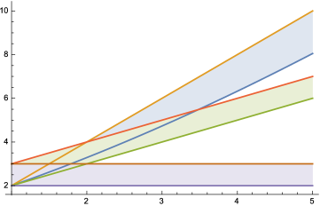
Figure 15: ${\cal L}_{1}$: the blue region; ${\cal L}_{2}$: the green region; ${\cal L}_{3}$: the violet region (Mathematica).

Using ${\cal P}$, the set ${\cal D}_{\rm s}$ becomes (at the expenses of diminishing $\varepsilon$, if necessary)

$${\cal D}_{\rm s}={\cal A}_{\rm s}\times{\cal B}_{\rm s}\times{{T}}^{3}$$

where, if

$${\cal L}_{\rm s}({C}):=\Big{\{}{\Lambda}=({\Lambda}_{1},{\Lambda}_{2})\in{\cal L}_{0}:\ |{\Lambda}_{2}-{\Lambda}_{1}-{C}|<\varepsilon\Big{\}}\ ,\qquad{\cal G}_{\rm s}({\Lambda}_{1}):=\Big{\{}\Theta_{1}:\ 0<{\Lambda}_{1}-\Theta_{1}<\varepsilon\Big{\}}\,,\$$ (342)

then

$${\cal A}_{\rm s}:=\Big{\{}({\Lambda}_{1},{\Lambda}_{2},\Theta_{1}):\ ({\Lambda}_{1},{\Lambda}_{2})\in{\cal L}_{\rm s}\ ,\ \Theta_{1}\in{\cal G}_{\rm s}({\Lambda}_{1})\Big{\}}\,,\ {\cal B}_{\rm s}:=\Big{\{}(\Theta_{2},\vartheta_{2}):\ |(\Theta_{2},\vartheta_{2})|<\varepsilon\Big{\}}\ .$$ (343)

All we have to do is to check that the intersection ${\cal A}_{\rm s}\cap{\cal A}_{\rm u}$ is non–empty.
Recalling the definition of ${\cal A}_{\rm u}$ in (2.3)–(2.3) and the definition of ${\cal A}_{\rm s}$ in (342)–(343), asserting that ${\cal A}_{\rm s}\cap{\cal A}_{\rm u}\neq\emptyset$ is equivalent to asserting that

$${\cal L}_{\rm s}({C})\cap{\cal L}_{\rm u}({C})\neq\emptyset$$

and

$${\cal G}_{\rm s}({\Lambda}_{1})\cap{\cal G}_{\rm u}({\Lambda}_{1},{\Lambda}_{2},{C})\neq\emptyset\quad\forall\ ({\Lambda}_{1},{\Lambda}_{2})\in{\cal L}_{\rm s}({C})\cap{\cal L}_{\rm u}({C})\ .$$

It will be enough to check that

$${\cal L}_{\rm s}({C})\cap{\cal L}_{\rm u}({C})\cap{\cal L}_{{\rm su}}({C})\neq\emptyset$$ (344)

and

$${\cal G}_{\rm s}({\Lambda}_{1})\cap{\cal G}_{\rm u}({\Lambda}_{1},{\Lambda}_{2},{C})\neq\emptyset\quad\forall\ ({\Lambda}_{1},{\Lambda}_{2})\in{\cal L}_{\rm s}({C})\cap{\cal L}_{\rm u}({C})\cap{\cal L}_{{\rm su}}({C})\ ,$$ (345)

where, if $\overline{C}_{\pm}$ are as in (337), ${\cal L}_{{\rm su}}$ is defined as

$${\cal L}_{{\rm su}}:=\Big{\{}({\Lambda}_{1},{\Lambda}_{2}):\ \overline{C}_{+}={\Lambda}_{1}\Big{\}}\ .$$ (346)

Note that (345) is certainly satisfied provided (344) is, since in fact, for $({\Lambda}_{1},{\Lambda}_{2})\in{\cal L}_{\rm s}({C})\cap{\cal L}_{\rm u}({C})\cap{\cal L}_{{\rm su}}({C})$,

$${\cal G}_{\rm s}({\Lambda}_{1})\cap{\cal G}_{\rm u}({\Lambda}_{1},{\Lambda}_{2},{C})=\Big{\{}\Theta_{1}:\ \max\{\overline{C}_{-},{\Lambda}_{1}-\varepsilon\}<\Theta_{1}<{\Lambda}_{1}\Big{\}}$$

which is well–defined by (337)–(338).

On the other hand, in view of the definition of $\overline{C}_{+}$ in (337), and of ${C}^{\star}$ a few lines above, ${\cal L}_{{\rm su}}$ in (346) is equivalently defined as

$${\cal L}_{{\rm su}}=\Big{\{}({\Lambda}_{1},{\Lambda}_{2}):\ 5{\Lambda}_{2}^{2}{C}-({C}+{\Lambda}_{1})^{2}(4{C}+{\Lambda}_{1})>0\Big{\}}\ .$$ (347)

Therefore, in view of this definition and the definitions of ${\cal L}_{\rm s}$, ${\cal L}_{\rm u}$ in (2.3) and (342), one sees that the set on the left hand side in (344) is determined by inequalities

$${\Lambda}_{-}<{\Lambda}_{1}<{\Lambda}_{+}$$

$$k_{-}{\Lambda}_{1}\leq{\Lambda}_{2}\leq k_{+}{\Lambda}_{1}$$

$$5{\Lambda}_{2}^{2}{C}-({C}+2\sqrt{{\alpha}_{+}}{\Lambda}_{2})^{2}(4{C}+2\sqrt{{\alpha}_{+}}{\Lambda}_{2})>0$$

$${\Lambda}_{1}>{C}$$

$${\Lambda}_{2}>\max\{{C}+2\sqrt{{\alpha}_{+}}{\Lambda}_{1},\ 2{C}\}$$

$$|{\Lambda}_{2}-{\Lambda}_{1}-{C}|<\varepsilon$$

$$5{\Lambda}_{2}^{2}{C}-({C}+{\Lambda}_{1})^{2}(4{C}+{\Lambda}_{1})>0$$ (348)

We observe that no phase point $({\Lambda}_{1},{\Lambda}_{2})$ with ${\Lambda}_{2}-{\Lambda}_{1}-{C}<0$ will ever satisfy (2.3), and that inequality ${\Lambda}_{2}>2{C}$ is implied by ${\Lambda}_{1}>{C}$ and (347). Then, we divide such inequalities in three groups, so as to rewrite the set (344) as the intersection of the sets

$$\mathaccent 866{{\cal L}}_{1} := \Big{\{}({\Lambda}_{1},{\Lambda}_{2}):\ {\Lambda}_{-}<{\Lambda}_{1}<{\Lambda}_{+},\ {\Lambda}_{1}>{C},\ {\Lambda}_{2}>2{C}\ ,$$

$$\max\{k_{-}{\Lambda}_{1},\ ({C}+{\Lambda}_{1})\sqrt{\frac{4{C}+{\Lambda}_{1}}{5{C}}}\}<{\Lambda}_{2}\leq k_{+}{\Lambda}_{1}\Big{\}}$$

$$\mathaccent 866{{\cal L}}_{2} := \Big{\{}({\Lambda}_{1},{\Lambda}_{2}):\ 0<{\Lambda}_{2}-{\Lambda}_{1}-{C}<\varepsilon,\ {\Lambda}_{2}>{C}+2\sqrt{{\alpha}_{+}}{\Lambda}_{1}\ ,\ {\Lambda}_{1}>{C}\Big{\}}$$

$$\mathaccent 866{{\cal L}}_{3} := \Big{\{}({\Lambda}_{1},{\Lambda}_{2}):\ 5{\Lambda}_{2}^{2}{C}-({C}+2\sqrt{{\alpha}_{+}}{\Lambda}_{2})^{2}(4{C}+2\sqrt{{\alpha}_{+}}{\Lambda}_{2})>0\ ,\ {\Lambda}_{2}>2{C}\Big{\}}$$

We now aim to choose the parameters ${\Lambda}_{\pm}$, $k_{\pm}$ and ${\alpha}_{+}$ so as to find a non–empty intersection of the sets a above.

Let us denote as ${\cal C}$ the curve, in the $({\Lambda}_{2},{\Lambda}_{1})$–plane, having equation

$${\cal C}:\qquad{\Lambda}_{2}=({C}+{\Lambda}_{1})\sqrt{\frac{4{C}+{\Lambda}_{1}}{5{C}}}$$ (349)

Let

$${\Lambda}_{1}=k{\Lambda}_{2}$$

be any straight line through the origin. The straight line intersecting ${\cal C}$ into the point $(\underline{{\Lambda}_{1}},\underline{{\Lambda}_{2}})=({C},2{C})$ has $\overline{k}=2$, and intersects this curve, also in the higher point

$$(\overline{{\Lambda}_{1}},\overline{{\Lambda}_{2}})=(\frac{1}{2}(13+\sqrt{185}),(13+\sqrt{185})){C}\ .$$

Any other line with $k>\overline{k}$ has a lower intersection $(\underline{{\Lambda}_{1}}^{\prime},\underline{{\Lambda}_{2}}^{\prime})$, with $\underline{{\Lambda}_{1}}^{\prime}<{C}$ and $\underline{{\Lambda}_{2}}^{\prime}<2{C}$ and a higher intersection $(\overline{{\Lambda}_{1}}^{\prime},\overline{{\Lambda}_{2}}^{\prime})$ with $\overline{{\Lambda}_{1}}^{\prime}>\overline{{\Lambda}_{1}}$ and $\overline{{\Lambda}_{2}}^{\prime}>\overline{{\Lambda}_{2}}$.

The last straight line, in the plane $({\Lambda}_{1},{\Lambda}_{2})$, through the origin intersecting ${\cal C}$ is the tangent line, and it is easy to compute (see below) that such a tangent line has slope has slope $\underline{k}$ as in (341) (Figure 13). We then conclude that, as soon as we choose $k_{-}<\underline{k}$, $k_{+}>\overline{k}$, ${\Lambda}_{-}<\underline{{\Lambda}_{1}}$, ${\Lambda}_{+}>\overline{{\Lambda}_{1}}$, we have the inclusion

$$\mathaccent 866{{\cal L}}_{1}\supset{\cal L}_{1}:=\Big{\{}({\Lambda}_{1},{\Lambda}_{2}):\ ({C}+{\Lambda}_{1})\sqrt{\frac{4{C}+{\Lambda}_{1}}{5{C}}}\}<{\Lambda}_{2}\leq 2{\Lambda}_{1}\Big{\}}\ .$$

Let us now turn to $\mathaccent 866{{\cal L}}_{2}$. Since we are assuming ${\alpha}_{+}<\frac{1}{16}$, we conclude that the strip

$${\cal L}_{2}:=\Big{\{}({\Lambda}_{1},{\Lambda}_{2}):\ 0<{\Lambda}_{2}-{\Lambda}_{1}-{C}<\varepsilon\ ,\ {\Lambda}_{1}>{C}\Big{\}}$$

is all included in the region

$$\mathaccent 869{{\cal L}}_{2}=\Big{\{}({\Lambda}_{1},{\Lambda}_{2}):\ {\Lambda}_{2}>{C}+2\sqrt{{\alpha}_{+}}{\Lambda}_{1}\ ,\ {\Lambda}_{1}>{C}\Big{\}}$$

and this allows to conclude

$$\mathaccent 866{{\cal L}}_{2}={\cal L}_{2}\cap\mathaccent 869{{\cal L}}_{2}={\cal L}_{2}\ .$$

Since the sets ${\cal L}_{1}$ and ${\cal L}_{2}$ have a non–empty intersection, independently of ${\alpha}_{+}$ (see Figure 14), a fortiori, $\mathaccent 866{{\cal L}}_{1}$ and $\mathaccent 866{{\cal L}}_{2}$ have one:

$$\mathaccent 866{{\cal L}}_{1}\cap\mathaccent 866{{\cal L}}_{2}\supset{\cal L}_{1}\cap{\cal L}_{2}\neq\emptyset\ .$$

Observe, in particular, that ${\cal L}_{1}\cap{\cal L}_{2}$ (hence, $\mathaccent 866{{\cal L}}_{1}\cap\mathaccent 866{{\cal L}}_{2}$) has non–empty intersection with any strip $\times\Big{[}2{C},y\Big{]}$, with $y>2{C}$ (see Figure 15).

On the other hand, it is immediate to check that $\mathaccent 866{{\cal L}}_{3}$ includes the horizontal strip

$${\cal L}_{3}:=\Big{\{}({\Lambda}_{1},{\Lambda}_{2}):\ 2{C}<{\Lambda}_{2}<\frac{{C}}{2\sqrt{{\alpha}_{+}}}\ ,\ {\Lambda}_{1}\in\Big{\}}\qquad 0<{\alpha}_{+}<\frac{1}{16}$$

and so we conclude

$${\cal L}_{\rm s}({C})\cap{\cal L}_{\rm u}({C})\cap{\cal L}_{{\rm su}}({C})=\mathaccent 866{{\cal L}}_{1}\cap\mathaccent 866{{\cal L}}_{2}\cap\mathaccent 866{{\cal L}}_{3}\supset{\cal L}_{1}\cap{\cal L}_{2}\cap{\cal L}_{3}\neq\emptyset$$

In order to complete the proof, it remains to prove that the tangent straight line to ${\cal C}$ through the origin has slope has slope $\underline{k}$ as in (341).
We switch to the homogenized variables

$$x:=\frac{{\Lambda}_{1}}{{C}}\qquad y=\frac{{\Lambda}_{2}}{{C}}$$

so that the curve ${\cal C}$ in (349) becomes

$$\mathaccent 866{{\cal C}}:\qquad y=(1+x)\sqrt{\frac{4+x}{5}}\ .$$

We look for a straight line through the origin $y=\underline{k}x$ with $\underline{k}>0$ which is tangent to $\mathaccent 866{{\cal C}}$ at some point $(a,b)$, with $a>0$.

The intersections between $\mathaccent 866{{\cal C}}$ and any straight line through the origin $y=kx$ are ruled by a complete cubic equation, given by

$$x^{3}+(6-5k^{2})x^{2}+9x+4=0\ .$$ (350)

In order that such an equation has a double solution $x=a$ for $k=\underline{k}$, one needs that, when $k=\underline{k}$, it can factorized as

$$(x-a)^{2}(x-c)=0$$ (351)

Therefore, equating the respective coefficients of (350) and (351) one finds the equations

$$\left\{\begin{array}[]{l}\displaystyle-(c+2a)=6-5\underline{k}^{2}\\ \\ \displaystyle 2ac+a^{2}=9\\ \\ \displaystyle-a^{2}c=4\end{array}\right.$$

Two last equations, allow to eliminate $b$ so as to obtain the equation for $a$

$$a^{3}-9a-8=0$$

which has the following three roots:

$$a_{0}=-1\ ,\qquad a_{\pm}=\frac{1\pm\sqrt{33}}{2}\ .$$

The only admissible (positive) value is then

$$a=a_{+}=\frac{1+\sqrt{33}}{2}$$

and it provides the values

$$c=\frac{-17+\sqrt{33}}{32}\ ,\qquad\underline{k}=\frac{1}{4}\sqrt{\frac{3}{10}(69+11\sqrt{33})}\ .\quad\square$$

Appendix A The $m_{0}$–centric reduction

The Hamiltonian of $1+n$ masses $m_{0}$, $\ldots$, $m_{n}$ interacting through gravity is

$${\cal H}=\sum_{i=0}^{n}\frac{|\mathbf{u}_{i}|^{2}}{2m_{i}}-\sum_{0\leq i<j\leq n}\frac{m_{i}m_{j}}{|\mathbf{v}_{i}-\mathbf{v}_{j}|}\,.$$ (352)

We switch from the position coordinates $\mathbf{v}_{i}$ to new new ones, denoted $\mathbf{x}_{i}$, where ${\mathbf{x}}_{0}$ is the coordinate of $m_{0}$, while ${\mathbf{x}}_{i}$ is the coordinate of $m_{i}$ relatively to $m_{0}$. The change is

$$\mathbf{v}_{i}=\left\{\begin{array}[]{lll}\mathbf{x}_{0}&i=0\\ \mathbf{x}_{i}+\mathbf{x}_{0}&i=1\,,\ldots\,,n\,.\end{array}\right.$$ (355)

As the change does not involve the $\mathbf{u}_{i}$’s, the coordinates ${\mathbf{y}}_{i}$ conjugated to $\bm{x}_{i}$ may be computed imposing the conservation of the standard 1–form

$${\Lambda}=\sum_{i=0}^{n}\bm{y}_{i}\cdot d\bm{x}_{i}=\sum_{i=0}^{n}\mathbf{u}_{i}\cdot d\mathbf{v}_{i}\,.$$

We find

$$\sum_{i=0}^{n}\mathbf{u}_{i}\cdot\mathbf{v}_{i} = \mathbf{u}_{0}\cdot\mathbf{x}_{0}+\sum_{i=1}^{n}\mathbf{u}_{i}\cdot(\mathbf{x}_{i}+{\mathbf{x}}_{0})$$

$$= \left(\sum_{i=0}^{n}\mathbf{u}_{i}\right)\cdot{\mathbf{x}}_{0}+\sum_{i=1}^{n}\mathbf{u}_{i}\cdot\mathbf{x}_{i}\,.$$

So we identify

$$\mathbf{y}_{i}=\left\{\begin{array}[]{lll}\displaystyle\sum_{i=0}^{n}\mathbf{u}_{i}&i=0\\ \\ \displaystyle\mathbf{u}_{i}&i=1\,,\ldots\,,n\,.\end{array}\right.$$

We recognize that ${\mathbf{y}}_{0}$ is the total linear momentum, which keeps constant along the motions of ${\cal H}$, as ${\cal H}$ is translation–invariant. Fixing a reference frame moving with the the centre of mass of $m_{0}$, $\ldots$, $m_{n}$, we have ${\mathbf{y}}_{0}=0$ and hence

$$\mathbf{u}_{i}=\left\{\begin{array}[]{lll}\displaystyle-\sum_{i=1}^{n}\mathbf{y}_{i}&i=0\\ \\ \displaystyle\mathbf{y}_{i}&i=1\,,\ldots\,,n\,.\end{array}\right.$$ (359)

Replacing (359) and (355) into (352) we arrive at (1), with $\mu_{i}$, $M_{i}$ as in (2).

References

- [1] V.I. Arnold. Small denominators and problems of stability of motion in classical and celestial mechanics. Russian Math. Surveys, 18(6):85–191, 1963.
- [2] L. Chierchia and G. Pinzari. Properly–degenerate KAM theory (following V.I. Arnold). Discrete Contin. Dyn. Syst. Ser. S, 3(4):545–578, 2010.
- [3] L. Chierchia and G. Pinzari. Deprit’s reduction of the nodes revised. Celestial Mech., 109(3):285–301, 2011.
- [4] L. Chierchia and G. Pinzari. Planetary Birkhoff normal forms. J. Mod. Dyn., 5(4):623–664, 2011.
- [5] L. Chierchia and G. Pinzari. The planetary -body problem: symplectic foliation, reductions and invariant tori. Invent. Math., 186(1):1–77, 2011.
- [6] L. Chierchia and G. Pinzari. Metric stability of the planetary n–body problem. Proceedings of the International Congress of Mathematicians, 2014.
- [7] A. Deprit. Elimination of the nodes in problems of bodies. Celestial Mech., 30(2):181–195, 1983.
- [8] J. Féjoz. Démonstration du ‘théorème d’Arnold’ sur la stabilité du système planétaire (d’après Herman). Ergodic Theory Dynam. Systems, 24(5):1521–1582, 2004.
- [9] R. S. Harrington. The stellar three-body problem. Celestial Mech. and Dyn. Astrronom, 1(2):200–209, 1969.
- [10] H. Hofer, E. Zehnder. Symplectic Invariants and Hamiltonian Dynamics. Birkhäuser Verlag, Basel, 1994.
- [11] G. Pinzari. On the Kolmogorov set for many–body problems. PhD thesis, Università Roma Tre, April 2009.
- [12] G. Pinzari. Aspects of the planetary Birkhoff normal form. Regul. Chaotic Dyn., 18(6):860–906, 2013.
- [13] G. Pinzari. On the co-existence of maximal and whiskered tori in the planetary three-body problem. J. Math. Phys., 59(5):052701, 37, 2018.
- [14] G. Pinzari. Perihelia reduction and global Kolmogorov tori in the planetary problem. Mem. Amer. Math. Soc., 255(1218), 2018.
- [15] J. Pöschel. Nekhoroshev estimates for quasi-convex Hamiltonian systems. Math. Z., 213(2):187–216, 1993.
- [16] R. Radau. Sur une transformation des équations différentielles de la dynamique. Ann. Sci. Ec. Norm. Sup., 5:311–375, 1868.