Mean-Field Approximation of Cooperative Constrained Multi-Agent Reinforcement Learning (CMARL)

Abstract

Mean-Field Control (MFC) has recently been proven to be a scalable tool to approximately solve large-scale multi-agent reinforcement learning (MARL) problems. However, these studies are typically limited to unconstrained cumulative reward maximization framework. In this paper, we show that one can use the MFC approach to approximate the MARL problem even in the presence of constraints. Specifically, we prove that, an $N$-agent constrained MARL problem, with state, and action spaces of each individual agents being of sizes $|\mathcal{X}|$, and $|\mathcal{U}|$ respectively, can be approximated by an associated constrained MFC problem with an error, $e\triangleq\mathcal{O}\left([\sqrt{|\mathcal{X}|}+\sqrt{|\mathcal{U}|}]/\sqrt{N}\right)$. In a special case where the reward, cost, and state transition functions are independent of the action distribution of the population, we prove that the error can be improved to $e=\mathcal{O}(\sqrt{|\mathcal{X}|}/\sqrt{N})$. Also, we provide a Natural Policy Gradient based algorithm, and prove that it can solve the constrained MARL problem within an error of $\mathcal{O}(e)$ with a sample complexity of $\mathcal{O}(e^{-6})$.

1 Introduction

Consider the situation of a policy-maker that is tasked with allocating a certain amount of budget to improve the health of a number of infrastructures in a post-disaster scenario. If, due to the repair, the health of a certain infrastructure improves, it provides the perception of a high reward to the planner. However, such improvement comes at the “cost" of the amount of money that is allocated to it. How should the planner allocate the money over a long-period of time? To answer such a question is same as assigning a policy to each infrastructure that states how much money should that infrastructure draw from the budget pool based on the global state of all infrastructures. The aim of designing such policies should be to maximize the expected cumulative reward while obeying the budget constraint.

Strategizing the decisions of a large pool of interacting agents under certain constraints is a frequently appearing problem in many branches of social science and engineering. For example, such framework can be applied for collision avoidance in self-driving cars (Fisac et al., 2018), safety precautions in robotic environment (Garcıa and Fernández, 2015) etc. A common way to deal with such problems is to use the framework of constrained multi-agent reinforcement learning (CMARL). In cooperative CMARL, the goal is to maximize the aggregate reward of the whole population while obeying some specified constraints. Unfortunately, as the number of agents increases, the size of the joint state-space increases exponentially, rendering the task of maximizing reward incredibly hard.

Note that the phenomena of state-space explosion is not unique to CMARL$-$unconstrained MARL problems also face the same issue. There have been a number of attempts to alleviate this obstacle. For example, one idea is to confine the policies to be local. This approach has yielded a number of useful algorithms e.g., Independent Q-Learning (IQL) (Tan, 1993), centralized training and decentralized execution (CTDE) (Son et al., 2019; Sunehag et al., 2017; Rashid et al., 2020, 2018) based algorithms, etc. Despite their empirical success, none of the above algorithms can provide theoretical guarantees. Another alternative is the framework of mean-field control (MFC) which builds upon the idea that in an infinite population of identical agents, studying one representative agent is sufficient to infer the statistics of their collective behaviour (Angiuli et al., 2022). MFC has recently been applied to approximate $N$-agent unconstrained MARL problems with theoretical guarantees (Gu et al., 2021). It is, however, still unknown whether similar approximation results can be established for CMARL problems. In this paper, we provide an affirmative answer to this question.

Establishing MFC-based approximation bounds for CMARL is particularly challenging for the following reason. Unlike in unconstrained MARL, the set of feasible policies of CMARL may not be identical to the sets of feasible policies of its associated constrained MFC (CMFC) problem. In general, a feasible policy for CMARL may overshoot the constraints of CMFC and vice versa. Clearly the sets of feasible policies of CMARL and CMFC may partially overlap but none is subset of another. The lack of structural hierarchy between the feasible policy sets makes it difficult to compare the optimal values of CMARL and CMFC. The trick is not to deal with the original CMARL, and CMFC problems but to consider variants of those with smaller feasible sets. We show that these variants can be judiciously chosen to enforce hierarchy, and thereby create a way to compare values.

1.1 Our Contribution

We consider an $N$-agent CMARL problem where at each instant the agents receive rewards as well as incur costs depending on their joint states, and actions. The goal is to maximize the time discounted sum of rewards (called reward-value or simple value) while ensuring that the discounted cumulative cost lie below a certain threshold. We show that the stated $N$-agent CMARL problem can be well approximated by a CMFC problem with an appropriately adjusted constraint. In particular, our result (Theorem 1) states that the optimal value of the stated CMFC is at most at the distance of $\mathcal{O}(e)$ from the optimal CMARL value where $e=\frac{1}{\sqrt{N}}[\sqrt{|\mathcal{X}|}+\sqrt{|\mathcal{U}|}]$. The terms $|\mathcal{X}|,|\mathcal{U}|$ denote the sizes of state, and action spaces of individual agents respectively. We also show that if the optimal policy obtained by solving the CMFC is adopted into the $N$-agent system, then it does not violate the constraint of CMARL, and yields an $N$-agent cumulative reward that is $\mathcal{O}(e)$ error away from the optimal $N$-agent value (Corollary 2). In a special case where the reward, cost, and state transition functions are independent of the action distribution of the population, we prove that the error improves to, $e=\sqrt{|\mathcal{X}|}/\sqrt{N}$ (Theorem 4).

The key idea behind Theorem 1 is a novel sandwiching technique. Specifically, we consider three distinct problems$-$ a CMARL with zero constraint bound (target problem), a CMFC with slightly more restrictive constraint, and a CMARL with even more restrictive constraint. We prove that the optimal value for the CMFC problem must be trapped between the optimal values of the CMARL problems with a small margin of error. Next, we establish that the CMARL values themselves must be close for large $N$. This forces the CMFC value to lie in the vicinity of our target value.

Finally, using the global convergence result of (Ding et al., 2020), we devise a natural policy gradient based primal-dual (NPG-PD) algorithm and show that the policy obtained from the stated algorithm satisfies the constraint of CMARL and approximates the optimal $N$-agent value within an error of $\mathcal{O}(e)$. The sample complexity of the algorithm is shown to be $\mathcal{O}(e^{-6})$ (Theorem 5).

1.2 Related Works

Unconstrained Single Agent RL: One of the early attempt to address the problem of single agent RL was made by the tabular Q-learning (Watkins and Dayan, 1992), and subsequently by the SARSA algorithm (Rummery and Niranjan, 1994). However, such approaches work only when the state space is small. Neural Network based Deep Q-learning (Mnih et al., 2015), and deep policy gradient algorithms (Li et al., 2019) have been introduced relatively recently to tackle large state space. One cannot, however, scale these approaches to large number of agents due to the exponential blow up of their joint state-space.

Constrained Single Agent RL: Decision making under constraint is typically modeled via Constrained Markov Decision Problems (CMDPs) (Chow et al., 2017). Several policy gradient (PG) or direct policy search methods have been proposed to solve CMDPs (Achiam et al., 2017; Bhatnagar and Lakshmanan, 2012; Liang et al., 2018). However, convergence guarantees of these algorithms are local. Recently, a series of PG-type algorithms have been proposed that ensure global convergence (Paternain et al., 2022; Ding et al., 2020). The advantage of mean-field approach is that it effectively reduces a multi-agent problem to a single agent problem, thereby allowing us to utilize these existing guarantees of CMDPs.

MFC-based Approximation of MARL: There have been a number of recent advances that show that MFC well-approximates MARL problems in the regime of large population. (Gu et al., 2021) showed that an $N$-agent homogeneous MARL problem can be approximated by MFC within $\mathcal{O}(\frac{1}{\sqrt{N}})$ error. (Mondal et al., 2022a) later extended this idea to heterogeneous MARL. Their approaches, however, cannot be directly adopted for CMARL. MFC has also been used to design local policies (Mondal et al., 2022c) and approximate cooperative MARL with non-uniform interactions (Mondal et al., 2022b).

Algorithms for MFC: In the model-free set up, both $Q$-learning based (Angiuli et al., 2022; Gu et al., 2021), and PG-based algorithms (Carmona et al., 2019) have been proposed to solve MFC problems. Model based algorithms are also available in the literature (Pasztor et al., 2021). However, none of these algorithms apply to CMFC problems.

Application of MFC: MFC has found its application in multitude of social and engineering applications ranging from epidemic control (Watkins et al., 2016; Lee et al., 2021), ride-hailing (Al-Abbasi et al., 2019), congestion management (Wang et al., 2020) etc.

2 Model for Cooperative CMARL

We consider a collection of $N$ agents interacting with each other in discrete time steps $t\in\{0,1,\cdots\}$. The state of $i$-th agent at time $t$ is denoted as $x_{t}^{i}$ which can take values from the finite state space, $\mathcal{X}$. The joint state of $N$-agents at time $t$ is symbolised as $\boldsymbol{x}_{t}^{N}\triangleq\{x_{t}^{i}\}_{i\in\{1,\cdots,N\}}$. Upon observing $\boldsymbol{x}_{t}^{N}$, the $i$-th agent chooses an action $u_{t}^{i}$ from the finite action set, $\mathcal{U}$ according to the following probability law: $u_{t}^{i}\sim\pi_{i}(\boldsymbol{x}_{t}^{N})$. The term, $\pi_{i}$, is said to be the policy of $i$-th agent, and defined to be a function of the following form, $\pi_{i}:\mathcal{X}^{N}\rightarrow\mathcal{P}(\mathcal{U})$ where $\mathcal{P}(\cdot)$ defines a probability simplex over its argument. The joint action of $N$-agents at time $t$ is indicated as $\boldsymbol{u}_{t}^{N}\triangleq\{u_{t}^{i}\}_{i\in\{1,\cdots,N\}}$. As a consequence of these actions, the $i$-th agent receives a reward $r_{i}(\boldsymbol{x}_{t}^{N},\boldsymbol{u}_{t}^{N})$, a constraint cost $c_{i}(\boldsymbol{x}_{t}^{N},\boldsymbol{u}_{t}^{N})$ at time $t$, and its state changes in the next time step according to the following transition rule: $x_{t+1}^{i}\sim P_{i}(\boldsymbol{x}_{t}^{N},\boldsymbol{u}_{t}^{N})$.

Note that, the reward, cost, and state transition law of an agent are not only affected by its own state, and action but also by states, and actions of other agents. Such interlacing is one of the main obstacles in solving large multi-agent problems. To ease the analysis, we shall assume a special structure of the reward, cost, and transition functions that are routinely adopted in the mean-field literature (Gu et al., 2021; Angiuli et al., 2022). Specifically, we assume that for some $r,c:\mathcal{X}\times\mathcal{U}\times\mathcal{P}(\mathcal{X})\times\mathcal{P}(\mathcal{U})\rightarrow\mathbb{R}$, and $P:\mathcal{X}\times\mathcal{U}\times\mathcal{P}(\mathcal{X})\times\mathcal{P}(\mathcal{U})\rightarrow\mathcal{P}(\mathcal{X})$, the following holds $\forall i\in\{1,\cdots,N\}$,

$$r_{i}(\boldsymbol{x}_{t}^{N},\boldsymbol{u}_{t}^{N})=r(x_{t}^{i},u_{t}^{i},\boldsymbol{\mu}_{t}^{N},\boldsymbol{\nu}_{t}^{N})$$ (1)

$$P_{i}(\boldsymbol{x}_{t}^{N},\boldsymbol{u}_{t}^{N})=P(x_{t}^{i},u_{t}^{i},\boldsymbol{\mu}_{t}^{N},\boldsymbol{\nu}_{t}^{N})$$ (2)

$$c_{i}(\boldsymbol{x}_{t}^{N},\boldsymbol{u}_{t}^{N})=c(x_{t}^{i},u_{t}^{i},\boldsymbol{\mu}_{t}^{N},\boldsymbol{\nu}_{t}^{N})$$ (3)

where $\boldsymbol{\mu}_{t}^{N}$, $\boldsymbol{\nu}_{t}^{N}$ denote the empirical $N$-agent state, and action distributions respectively. Formally,

$$\boldsymbol{\mu}_{t}^{N}=\dfrac{1}{N}\sum_{i=1}^{N}\delta(x_{t}^{i}=x),~{}\forall x\in\mathcal{X},~{}~{}\text{and}~{}~{}\boldsymbol{\nu}_{t}^{N}=\dfrac{1}{N}\sum_{i=1}^{N}\delta(u_{t}^{i}=u),~{}\forall u\in\mathcal{U}$$ (4)

where $\delta(\cdot)$ is the indicator function. The equations $(\ref{eq_1})-(\ref{eq_3})$ are applicable to a system where agents are identical and exchangeable (Mondal et al., 2022a). These relations suggests that the effect of the population on any agent is mediated only through the mean-field distributions. We would also like to point out that the functions, $r$, $P$, and $c$ are identical for all agents. Therefore, the system of agents described above is essentially homogeneous. As a consequence, we can rewrite the policy functions, $\pi_{i}$ as follows for some $\pi:\mathcal{X}\times\mathcal{P}(\mathcal{X})\rightarrow\mathcal{P}(\mathcal{U})$, and $\forall i\{1,\cdots,N\}$,

$$\pi_{i}(\boldsymbol{x}_{t}^{N})=\pi(x_{t}^{i},\boldsymbol{\mu}_{t}^{N})$$ (5)

In simple words, due to homogeneity, we can describe the policy of an agent as a (stochastic) process of choosing its action upon observing its own state, and the state distribution of the whole population. The policy of an agent at time $t$ is denoted as $\pi_{t}$ where its sequence is denoted as $\boldsymbol{\pi}\triangleq\{\pi_{t}\}_{t\in\{0,1,\cdots\}}$. For a given initial joint state, $\boldsymbol{x}^{N}_{0}$, the $N$-agent reward, and cost-value (indicated respectively as $V^{R}_{N}$, $V^{C}_{N}$) of a policy-sequence $\boldsymbol{\pi}$ are defined as follows.

$$V^{R}_{N}(\boldsymbol{x}^{N}_{0},\boldsymbol{\pi})\triangleq\sum_{t=0}^{\infty}\gamma^{t}\mathbb{E}\left[\dfrac{1}{N}\sum_{i=1}^{N}r(x_{t}^{i},u_{t}^{i},\boldsymbol{\mu}_{t}^{N},\boldsymbol{\nu}_{t}^{N})\right]$$ (6)

$$V^{C}_{N}(\boldsymbol{x}^{N}_{0},\boldsymbol{\pi})\triangleq\sum_{t=0}^{\infty}\gamma^{t}\mathbb{E}\left[\dfrac{1}{N}\sum_{i=1}^{N}c(x_{t}^{i},u_{t}^{i},\boldsymbol{\mu}_{t}^{N},\boldsymbol{\nu}_{t}^{N})\right]$$ (7)

where the expectation is computed over all joint state-action trajectories induced by $\boldsymbol{\pi}$, and $\gamma\in[0,1)$ is a discount factor. Let, the set of all admissible policies be $\Pi$, and $\Pi_{\infty}\triangleq\Pi\times\Pi\times\cdots$ be the collection of all admissible policy sequences. The goal of $N$-agent CMARL is to solve the following optimization problem for a given initial joint state $\boldsymbol{x}_{0}^{N}$.

$$\begin{split}\sup_{\boldsymbol{\pi}\in\Pi_{\infty}}&~{}V_{N}^{R}(\boldsymbol{x}^{N}_{0},\boldsymbol{\pi})~{}~{}~{}~{}\mathrm{subject~{}to}:~{}V_{N}^{C}(\boldsymbol{x}^{N}_{0},\boldsymbol{\pi})\leq 0\end{split}$$ (CMARL)

We shall denote the solution to (CMARL) as $\boldsymbol{\pi}^{*}_{N}$. Obtaining a solution of (CMARL), is, in general, difficult. In the next section, we shall demonstrate how $\boldsymbol{\pi}^{*}_{N}$ can be approximated via constrained mean field control (CMFC) approach.

3 Model for Constrained Mean-Field Control (CMFC)

A mean-field system comprises of an infinite collection of agents. Due to homogeneity, it is sufficient to track only a representative agent to describe to the behaviour of the population. Let, the state, and action of this representative at time $t$ be denoted as $x_{t}\in\mathcal{X}$, $u_{t}\in\mathcal{U}$ respectively while the distributions of states, and actions of the whole population be denoted as $\boldsymbol{\mu}_{t}^{\infty}\in\mathcal{P}(\mathcal{X})$, and $\boldsymbol{\nu}_{t}^{\infty}\in\mathcal{P}(\mathcal{U})$. Observe that, for a given policy sequence, $\boldsymbol{\pi}\triangleq\{\pi_{t}\}_{t\in\{0,1,\cdots\}}$, the action distribution, $\boldsymbol{\nu}_{t}^{\infty}$ can be derived from the state distribution, $\boldsymbol{\mu}_{t}^{\infty}$ as follows.

$$\boldsymbol{\nu}_{t}^{\infty}=\nu^{\mathrm{MF}}(\boldsymbol{\mu}_{t}^{\infty},\pi_{t})\triangleq\sum_{x\in\mathcal{X}}\pi_{t}(x,\boldsymbol{\mu}_{t}^{\infty})\boldsymbol{\mu}_{t}^{\infty}(x)$$ (8)

Similarly, the state distribution at time $t+1$ can be obtained from $\boldsymbol{\mu}_{t}^{\infty}$ using the following update equation.

$$\boldsymbol{\mu}_{t+1}^{\infty}=P^{\mathrm{MF}}(\boldsymbol{\mu}_{t}^{\infty},\pi_{t})\triangleq\sum_{x\in\mathcal{X}}\sum_{u\in\mathcal{U}}P(x,u,\boldsymbol{\mu}_{t}^{\infty},\nu^{\mathrm{MF}}(\boldsymbol{\mu}_{t}^{\infty},\pi_{t}))\pi_{t}(x,\boldsymbol{\mu}_{t}^{\infty})(u)\boldsymbol{\mu}_{t}^{\infty}(x)$$ (9)

Finally, the average reward, and constraint cost at time $t$ can be computed as shown below.

$$r^{\mathrm{MF}}(\boldsymbol{\mu}_{t}^{\infty},\pi_{t})=\sum_{x\in\mathcal{X}}\sum_{u\in\mathcal{U}}r(x,u,\boldsymbol{\mu}_{t}^{\infty},\nu^{\mathrm{MF}}(\boldsymbol{\mu}_{t}^{\infty},\pi_{t}))\pi_{t}(x,\boldsymbol{\mu}_{t}^{\infty})(u)\boldsymbol{\mu}_{t}^{\infty}(x)$$ (10)

$$c^{\mathrm{MF}}(\boldsymbol{\mu}_{t}^{\infty},\pi_{t})=\sum_{x\in\mathcal{X}}\sum_{u\in\mathcal{U}}c(x,u,\boldsymbol{\mu}_{t}^{\infty},\nu^{\mathrm{MF}}(\boldsymbol{\mu}_{t}^{\infty},\pi_{t}))\pi_{t}(x,\boldsymbol{\mu}_{t}^{\infty})(u)\boldsymbol{\mu}_{t}^{\infty}(x)$$ (11)

For an initial state distribution, $\boldsymbol{\mu}_{0}^{\infty}=\boldsymbol{\mu}_{0}$, and a policy-sequence $\boldsymbol{\pi}$, we define value functions related to reward, and constraint cost as follows.

$$V^{R}_{\infty}(\boldsymbol{\mu}_{0},\boldsymbol{\pi})=\sum_{t=0}^{\infty}\gamma^{t}r^{\mathrm{MF}}(\boldsymbol{\mu}_{t}^{\infty},\pi_{t})$$ (12)

$$V^{C}_{\infty}(\boldsymbol{\mu}_{0},\boldsymbol{\pi})=\sum_{t=0}^{\infty}\gamma^{t}c^{\mathrm{MF}}(\boldsymbol{\mu}_{t}^{\infty},\pi_{t})$$ (13)

The goal of CMFC is to solve the following optimization problem.

$$\begin{split}\sup_{\boldsymbol{\pi}\in\Pi_{\infty}}&~{}V_{\infty}^{R}(\boldsymbol{\mu}_{0},\boldsymbol{\pi})~{}~{}~{}~{}\mathrm{subject~{}to}:~{}V_{\infty}^{C}(\boldsymbol{\mu}_{0},\boldsymbol{\pi})\leq 0\end{split}$$ (CMFC)

where $\Pi_{\infty}$, as stated in section 2, is the collection of admittable policy sequences. In the forthcoming section, we shall prove that the solution of a variant of (CMFC) closely approximates the solution of (CMARL) for large $N$.

4 Main Result: Approximation of CMARL via CMFC

Before stating the approximation result, we would like to enlist the set of assumptions that are needed to establish it. Our first assumption is on the reward, $r$, cost, $c$, and the state transition function, $P$.

Assumption 1

There exists constants $M_{R},M_{C},L_{R},L_{C},L_{P}>0$ such that the following relations hold $\forall x\in\mathcal{X}$, $\forall u\in\mathcal{U}$, $\forall\boldsymbol{\mu}_{1},\boldsymbol{\mu}_{2}\in\mathcal{P}(\mathcal{X})$, and $\forall\boldsymbol{\nu}_{1},\boldsymbol{\nu}_{2}\in\mathcal{P}(\mathcal{U})$.

$$(a)|r(x,u,\boldsymbol{\mu}_{1},\boldsymbol{\nu}_{1})|\leq M_{R},$$

$$(b)|c(x,u,\boldsymbol{\mu}_{1},\boldsymbol{\nu}_{1})|\leq M_{C},$$

$$(c)|r(x,u,\boldsymbol{\mu}_{1},\boldsymbol{\nu}_{1})-r(x,u,\boldsymbol{\mu}_{2},\boldsymbol{\nu}_{2})|\leq L_{R}\left[|\boldsymbol{\mu}_{1}-\boldsymbol{\mu}_{2}|_{1}+|\boldsymbol{\nu}_{1}-\boldsymbol{\nu}_{2}|_{1}\right],$$

$$(d)|c(x,u,\boldsymbol{\mu}_{1},\boldsymbol{\nu}_{1})-c(x,u,\boldsymbol{\mu}_{2},\boldsymbol{\nu}_{2})|\leq L_{C}\left[|\boldsymbol{\mu}_{1}-\boldsymbol{\mu}_{2}|_{1}+|\boldsymbol{\nu}_{1}-\boldsymbol{\nu}_{2}|_{1}\right],$$

$$(e)|P(x,u,\boldsymbol{\mu}_{1},\boldsymbol{\nu}_{1})-P(x,u,\boldsymbol{\mu}_{2},\boldsymbol{\nu}_{2})|_{1}\leq L_{P}\left[|\boldsymbol{\mu}_{1}-\boldsymbol{\mu}_{2}|_{1}+|\boldsymbol{\nu}_{1}-\boldsymbol{\nu}_{2}|_{1}\right]$$

where $|\cdot|_{1}$ denotes $L_{1}$-distance.

Assumption 1(a), and 1(b) states that the reward, $r$, and the cost function, $c$ are bounded. The very definition of the transition function, $P$ makes it bounded. Hence, it is not listed as an assumption. On the other hand, Assumption 1(c)-(e) dictate that the functions $r$, $c$, and $P$ are Lipschitz continuous with respect to their state, and action distribution arguments. Assumption 1 is common in the literature (Angiuli et al., 2022; Carmona et al., 2018). Our next assumption is on the class of admissible policies, $\Pi$.

Assumption 2

There exists a constant $L_{Q}>0$ such that $\forall\pi\in\Pi$ the following inequality holds.

$$|\pi(x,\boldsymbol{\mu}_{1})-\pi(x,\boldsymbol{\mu}_{2})|\leq L_{Q}|\boldsymbol{\mu}_{1}-\boldsymbol{\mu}_{2}|_{1}$$

$\forall x\in\mathcal{X}$, and $\forall\boldsymbol{\mu}_{1},\boldsymbol{\mu}_{2}\in\mathcal{P}(\mathcal{X})$.

Assumption 2 dictates that the admissible policies are Lipschitz continuous with respect to the state distributions. The assumption stated above is also common in the literature and holds for neural network based policies with bounded weights (Gu et al., 2021; Pasztor et al., 2021). Before stating the main result, we need to introduce some notations. Consider the following optimization problem.

$$\begin{split}\sup_{\boldsymbol{\pi}\in\Pi_{\infty}}&~{}V_{N}^{R}(\boldsymbol{x}^{N}_{0},\boldsymbol{\pi})~{}~{}~{}~{}\mathrm{subject~{}to}:~{}V_{N}^{C}(\boldsymbol{x}^{N}_{0},\boldsymbol{\pi})\leq\zeta\end{split}$$ (G-CMARL)

Problem (G-CMARL) is a generalization of problem (CMARL). Specifically, it uses an arbitrary real, $\zeta\in\mathbb{R}$, as the constraint upper bound, instead of $\zeta=0$ as considered in (CMARL). With slight abuse of notation, we define the optimal objective value of (G-CMARL) as $V_{N}^{*}(\boldsymbol{x}_{0}^{N},\zeta)$. In a similar fashion, $V_{\infty}^{*}(\boldsymbol{\mu}_{0},\zeta)$ denotes the optimal objective value of the following optimization problem for $\zeta\in\mathbb{R}$.

$$\begin{split}\sup_{\boldsymbol{\pi}\in\Pi_{\infty}}&~{}V_{\infty}^{R}(\boldsymbol{\mu}_{0},\boldsymbol{\pi})~{}~{}~{}~{}\mathrm{subject~{}to}:~{}~{}V_{\infty}^{C}(\boldsymbol{\mu}_{0},\boldsymbol{\pi})\leq\zeta\end{split}$$ (G-CMFC)

Clearly, (G-CMFC) generalizes the problem, (CMFC). The following Assumption is required (in Addition to Assumption 1, 2) to establish the main result.

Assumption 3

There exists $\zeta_{0}<0$ such that the set of feasible solutions of (G-CMARL) for $\zeta=\zeta_{0}$ is non-empty. In other words, there exists a policy-sequence, $\boldsymbol{\pi}\in\Pi_{\infty}$ such that $V_{N}^{C}(\boldsymbol{x}_{0}^{N},\boldsymbol{\pi})\leq\zeta_{0}$ for any given joint initial state, $\boldsymbol{x}_{0}^{N}$.

Assumption 3 ensures that no pathological example with empty feasible set arise in our analysis. This assumption is similar to Slater’s condition in the optimization literature. Below we state our result.

Theorem 1

Let $\boldsymbol{x}_{0}^{N}$ be the initial joint state in an $N$-agent system, and $\boldsymbol{\mu}_{0}$ its empirical distribution. If Assumptions $\ref{assumption_1}-\ref{assumption_2}$ hold, then there exists $N_{0}>0$ such that $\forall N\geq N_{0}$ the following inequality holds whenever $\gamma S_{P}<1$.

$$|V_{N}^{*}(\boldsymbol{x}_{0}^{N},0)-V_{\infty}^{*}(\boldsymbol{\mu}_{0},-G_{C})|\leq G_{R}+G_{C}\left[\dfrac{4}{\zeta_{0}}\left(\dfrac{M_{R}}{1-\gamma}\right)\right]$$ (14)

The terms $G_{R},G_{C}$ are defined as shown below.

$$G_{J}\triangleq\left(\dfrac{1}{1-\gamma}\right)\left[\dfrac{M_{J}}{\sqrt{N}}+\dfrac{L_{J}\sqrt{|\mathcal{U}|}}{\sqrt{N}}\right]+\dfrac{\left[\sqrt{|\mathcal{X}|}+\sqrt{|\mathcal{U}|}\right]}{\sqrt{N}}\left(\dfrac{S_{J}C_{P}}{S_{P}-1}\right)\left[\dfrac{1}{1-\gamma S_{P}}-\dfrac{1}{1-\gamma}\right]$$ (15)

where $C_{P}\triangleq 2+L_{P}$, $S_{J}\triangleq(M_{J}+2L_{J})+L_{Q}(M_{J}+L_{J})$, $S_{P}\triangleq(1+2L_{J})+L_{Q}(1+L_{J})$, and $J\in\{R,C\}$. The terms $\{M_{R},M_{C},L_{R},L_{C},L_{P},\zeta_{0}\}$ are defined in Assumptions 1, 2, and 3.

Theorem 1 provides a recipe for approximately solving the $N$-agent constrained MARL problem (CMARL). In particular, inequality $(\ref{eq_15})$ ensures that the optimal value function of $N$-agent problem (CMARL), and that of generalized constrained mean-field problem (G-CMFC) for $\zeta=-G_{C}$ are $\mathcal{O}(G_{R}+G_{C})$ distance away from each other. Note that $G_{R},G_{C}=\mathcal{O}\left(\frac{1}{\sqrt{N}}\right)$. Thus for sufficiently large $N$, obtaining a solution for (G-CMFC) for $\zeta=-G_{C}$ is approximately equivalent to solving the original $N$-agent problem (CMARL). We would like to mention that, $G_{R},G_{C}=\mathcal{O}(\sqrt{|\mathcal{X}|}+\sqrt{|\mathcal{U}|})$ where $|\mathcal{X}|,|\mathcal{U}|$ denote the sizes of state, and action spaces respectively. Therefore, as the state, and action spaces of individual agents become larger, the approximation progressive becomes worse.

Although $(\ref{eq_15})$ establishes the proximity of the value-functions of $N$-agent, and infinite agent systems, it does not clarify whether the policy-sequence obtained by solving (G-CMFC) for $\zeta=-G_{C}$ would obey the constraint of (CMARL) if the policy is adopted in an $N$-agent system. It also does not comment on how the said policy-sequence would perform (in terms of cumulative reward) in an $N$-agent system in comparison to the optimal $N$-agent value. These important questions are answered in the following Corollary. The proof of corollary 2 is relegated to Appendix A.

Corollary 2

Let $\boldsymbol{\pi}^{*}_{N}$, $\boldsymbol{\pi}^{*}_{\infty}$ be solutions of (CMARL), and (G-CMFC) with $\zeta=-G_{C}$ respectively. If Assumptions $\ref{assumption_1}-\ref{assumption_2}$ hold, then the following inequality holds for $\forall N\geq N_{0}$ whenever $\gamma S_{P}<1$.

$$V_{N}^{R}(\boldsymbol{x}_{0}^{N},\boldsymbol{\pi}_{N}^{*})-V_{N}^{R}(\boldsymbol{x}_{0}^{N},\boldsymbol{\pi}^{*}_{\infty})\leq 2G_{R}+G_{C}\left[\dfrac{4}{\zeta_{0}}\left(\dfrac{M_{R}}{1-\gamma}\right)\right],$$ (16)

and $$V_{N}^{C}(\boldsymbol{x}_{0}^{N},\boldsymbol{\pi}_{\infty}^{*})\leq 0$$ (17)

where $V_{N}^{R}(\cdot,\cdot)$, and $V_{N}^{C}(\cdot,\cdot)$ are defined in $(\ref{eq_def_v_r})$, and $(\ref{eq_def_v_c})$ respectively. The notations $\boldsymbol{x}_{0}^{N}$, $\boldsymbol{\mu}_{0}$, $G_{R}$, $G_{C}$, $S_{P}$, and $N_{0}$ carry the same meaning as stated in Theorem 1.

Inequalities $(\ref{eq_17}),(\ref{eq_18})$ dictate that if the policy-sequence, $\boldsymbol{\pi}^{*}_{\infty}$, obtained by solving the mean-field problem (G-CMFC) for $\zeta=-G_{C}$ is adopted in the $N$-agent system, then the value obtained for such a system is $\mathcal{O}(\frac{1}{\sqrt{N}})$ error away from the optimum. Also, $\boldsymbol{\pi}_{\infty}^{*}$ does not violate (CMARL) constraint.

5 Proof of Theorem 1

The proof of Theorem 1 hinges on Lemma 3. The proof of Lemma 3 is relegated to Appendix B.

Lemma 3

Let $\boldsymbol{x}_{0}^{N}$ be the initial joint state in an $N$-agent system, and $\boldsymbol{\mu}_{0}$ its empirical distribution. If Assumption $\ref{assumption_1}-\ref{assumption_2}$ hold, then there exists $N_{0}>0$ such that $\forall N\geq N_{0}$, and $\forall\boldsymbol{\pi}\in\Pi_{\infty}$, the following inequalities hold whenever $\gamma S_{P}<1$.

$$|V_{N}^{J}(\boldsymbol{x}_{0}^{N},\boldsymbol{\pi})-V_{\infty}^{J}(\boldsymbol{\mu}_{0},\boldsymbol{\pi})|\leq G_{J}$$ (18)

where $J\in\{R,C\}$. The value functions $V_{N}^{R},V_{N}^{C},V_{\infty}^{R},V_{\infty}^{C}$ are given by $(\ref{eq_def_v_r}),(\ref{eq_def_v_c})$, $(\ref{eq:v_r_mf}),(\ref{eq:v_c_mf})$ respectively, and the terms $G_{R},G_{C},S_{P}$ are defined in Theorem 1.

Intuitively, Lemma 3 dictates that the value function pairs $(V_{N}^{R},V_{\infty}^{R})$, $(V_{N}^{C},V_{\infty}^{C})$ are close in the sense that for every policy-sequence $\boldsymbol{\pi}$, the differences $|V_{N}^{J}(\boldsymbol{x}_{0}^{N},\boldsymbol{\pi})-V_{\infty}^{J}(\boldsymbol{\mu}_{0},\boldsymbol{\pi})|,|V_{N}^{J}(\boldsymbol{x}_{0}^{N},\boldsymbol{\pi})-V_{\infty}^{J}(\boldsymbol{\mu}_{0},\boldsymbol{\pi})|$, $J\in\{R,C\}$ are of the form $\mathcal{O}(\frac{1}{\sqrt{N}})$. Below we explain how such result helps us to establish Theorem 1. Consider the three distinct constrained maximizations stated below.

• Problem $0$: (G-CMARL) with $\zeta=0$. It is same as the original $N$-agent problem (CMARL).

• Problem $1$: (G-CMFC) with $\zeta=-G_{C}$.

• Problem $2$: (G-CMARL) with $\zeta=-2G_{C}$.

Let, $\Pi_{\infty}^{k}\subset\Pi_{\infty}$ be the set of admissible policy sequences that satisfy the constraint of $k$-th optimization problem stated above, $k\in\{0,1,2\}$. Note that, if $\boldsymbol{\pi}\in\Pi_{\infty}^{2}$, then

$$V_{\infty}^{C}(\boldsymbol{\mu}_{0},\boldsymbol{\pi})\overset{(a)}{\leq}V_{N}^{C}(\boldsymbol{x}_{0}^{N},\boldsymbol{\pi})+G_{C}\overset{(b)}{\leq}-G_{C}$$ (19)

Inequality $(a)$ follows from $(\ref{eq_19})$ and $(b)$ is a consequence of the fact that $\boldsymbol{\pi}\in\Pi_{\infty}^{2}$. Thus, $\Pi_{\infty}^{2}\subset\Pi_{\infty}^{1}$. Similarly, if $\boldsymbol{\pi}\in\Pi_{\infty}^{1}$, then

$$V_{N}^{C}(\boldsymbol{x}_{0}^{N},\boldsymbol{\pi})\overset{(a)}{\leq}V_{\infty}^{C}(\boldsymbol{\mu}_{0},\boldsymbol{\pi})+G_{C}\overset{(b)}{\leq}0$$ (20)

which shows $\Pi_{\infty}^{1}\subset\Pi_{\infty}^{0}$. Combining, we get $\Pi_{\infty}^{2}\subset\Pi_{\infty}^{1}\subset\Pi_{\infty}^{0}$. Finally, assume that $\boldsymbol{\pi}^{*}_{k}\in\Pi_{\infty}^{k}$ indicate the solution of $k$-th maximization problem described above, $k\in\{0,1,2\}$. Then,

$$V_{\infty}^{R}(\boldsymbol{\mu}_{0},\boldsymbol{\pi}_{1}^{*})\overset{(a)}{\leq}V_{N}^{R}(\boldsymbol{x}_{0}^{N},\boldsymbol{\pi}^{*}_{1})+G_{R}\overset{(b)}{\leq}V_{N}^{R}(\boldsymbol{x}_{0}^{N},\boldsymbol{\pi}^{*}_{0})+G_{R}=V_{N}^{*}(\boldsymbol{x}_{0}^{N},0)+G_{R},$$ (21)

$$V_{\infty}^{R}(\boldsymbol{\mu}_{0},\boldsymbol{\pi}_{1}^{*})\overset{(c)}{\geq}V_{\infty}^{R}(\boldsymbol{\mu}_{0},\boldsymbol{\pi}_{2}^{*})\overset{(d)}{\geq}V_{N}^{R}(\boldsymbol{x}_{0}^{N},\boldsymbol{\pi}^{*}_{2})-G_{R}=V_{N}^{*}(\boldsymbol{x}_{0}^{N},-2G_{C})-G_{R}$$ (22)

Inequalities (a), and (d) follow from $(\ref{eq_19})$. Relation $(b)$ is a consequence of the fact that $\boldsymbol{\pi}_{0}^{*}$ is a maximizer of $V_{N}^{R}(\boldsymbol{x}_{0}^{N},\cdot)$ over $\Pi_{\infty}^{0}$, and $\boldsymbol{\pi}_{1}^{*}\in\Pi_{\infty}^{1}\subset\Pi_{\infty}^{0}$. Similarly, $\boldsymbol{\pi}_{1}^{*}$ is a maximizer of $V_{\infty}^{R}(\boldsymbol{\mu}_{0},\cdot)$ over $\Pi_{\infty}^{1}$, and $\boldsymbol{\pi}_{2}^{*}\in\Pi_{\infty}^{2}\subset\Pi_{\infty}^{1}$. This establishes relation (c).

The gist of the above exercise is that the value $V_{\infty}^{*}(\boldsymbol{\mu}_{0},-G_{C})$ is sandwiched between $V_{N}^{*}(\boldsymbol{x}_{0}^{N},0)+G_{R}$, and $V_{N}^{*}(\boldsymbol{x}_{0}^{N},-2G_{C})-G_{R}$. To prove $(\ref{eq_15})$, we need to bound the distance between $V_{N}^{*}(\boldsymbol{x}_{0}^{N},0)$, and $V_{N}^{*}(\boldsymbol{x}_{0}^{N},-2G_{C})$. This can be accomplished using the concavity property of $V_{N}^{*}(\boldsymbol{x}_{0}^{N},\cdot)$ in the domain $[-\zeta_{0},0]$ where $\zeta_{0}$ is given in Assumption 3. The concavity property is a consequence of Proposition 1 of (Paternain et al., 2019). If $N\geq N_{0}$ where $N_{0}$ is a sufficiently large value, then $2G_{C}<\zeta_{0}$. In such a case,

$$V_{N}^{*}(\boldsymbol{x}_{0}^{N},-2G_{C})\geq\left(1-\dfrac{2G_{C}}{\zeta_{0}}\right)V_{N}^{*}(\boldsymbol{x},0)+\dfrac{2G_{C}}{\zeta_{0}}V_{N}^{*}(\boldsymbol{x}_{0}^{N},-\zeta_{0})$$

Equivalently, $$V_{N}^{*}(\boldsymbol{x}_{0}^{N},0)-V_{N}^{*}(\boldsymbol{x},-2G_{C})\leq\dfrac{2G_{C}}{\zeta_{0}}\left[V_{N}^{*}(\boldsymbol{x}_{0}^{N},0)-V_{N}^{*}(\boldsymbol{x}_{0}^{N},-\zeta_{0})\right]$$

Using Assumption 1(a), one can trivially deduce, $|V_{N}^{*}(\boldsymbol{x}_{0}^{N},\zeta)|\leq M_{R}/(1-\gamma)$, $\forall\zeta>\zeta_{0}$. Hence,

$$V_{N}^{*}(\boldsymbol{x}_{0}^{N},0)-V_{N}^{*}(\boldsymbol{x}_{0}^{N},-2G_{C})\leq G_{C}\left[\dfrac{4}{\zeta_{0}}\left(\dfrac{M_{R}}{1-\gamma}\right)\right]$$ (23)

Using $(\ref{eq23}),(\ref{eq_22})$, we obtain,

$$V_{N}^{*}(\boldsymbol{x}_{0}^{N},0)-V_{\infty}^{*}(\boldsymbol{\mu}_{0},-G_{C})\leq G_{R}+G_{C}\left[\dfrac{4}{\zeta_{0}}\left(\dfrac{M_{R}}{1-\gamma}\right)\right]$$ (24)

Combining with $(\ref{eq22})$, we conclude the result.

6 Improvement of Optimality Gap in a Special Case

In this section, we shall impose the following additional restriction on the structure of reward, $r$, cost, $c$, and transition function, $P$ to improve the approximation bound of Theorem 1.

Assumption 4

The functions $r$, $c$, and $P$ are independent of the action distribution of the population. Mathematically, $\forall x\in\mathcal{X}$, $\forall u\in\mathcal{U}$, $\forall\boldsymbol{\mu}\in\mathcal{P}(\mathcal{X})$, and $\forall\boldsymbol{\nu}\in\mathcal{P}(\mathcal{U})$,

$$(a)~{}r(x,u,\boldsymbol{\mu},\boldsymbol{\nu})=r(x,u,\boldsymbol{\mu}),(b)~{}c(x,u,\boldsymbol{\mu},\boldsymbol{\nu})=c(x,u,\boldsymbol{\mu}),~{}(c)~{}P(x,u,\boldsymbol{\mu},\boldsymbol{\nu})=P(x,u,\boldsymbol{\mu})$$

Assumption 4 removes the dependence of $r,c$, and $P$ on the action distribution. However, for each individual agent, those functions still take the action taken by the agent as an argument. Below we present our improved approximation result.

Theorem 4

Let $\boldsymbol{x}_{0}^{N}$ be the initial joint state in an $N$-agent system, and $\boldsymbol{\mu}_{0}$ its empirical distribution. If Assumptions $\ref{assumption_1}-\ref{assumption_3}$ hold, then there exists $N_{0}>0$ such that $\forall N\geq N_{0}$ the following inequality holds whenever $\gamma S_{P}<1$.

$$|V_{N}^{*}(\boldsymbol{x}_{0}^{N},0)-V_{\infty}^{*}(\boldsymbol{\mu}_{0},-G_{C}^{0})|\leq G_{R}^{0}+G_{C}^{0}\left[\dfrac{4}{\zeta_{0}}\left(\dfrac{M_{R}}{1-\gamma}\right)\right]$$ (25)

The terms $G_{R}^{0},G_{C}^{0}$ are defined as shown below.

$$G_{J}^{0}\triangleq\dfrac{M_{J}}{\sqrt{N}}\left(\dfrac{1}{1-\gamma}\right)+\dfrac{\sqrt{|\mathcal{X}|}}{\sqrt{N}}\left(\dfrac{2S_{J}}{S_{P}-1}\right)\left[\dfrac{1}{1-\gamma S_{P}}-\dfrac{1}{1-\gamma}\right]$$ (26)

where $J\in\{R,C\}$, and the terms $M_{R},M_{C},S_{R},S_{C},S_{P},\zeta_{0}$ are clarified in Theorem 1. Additionally, if $\boldsymbol{\pi}_{\infty}^{*}$ is a solution of (G-CMFC) with $\zeta=-G_{C}^{0}$, then the following inequalities hold $\forall N\geq N_{0}$ whenever $\gamma S_{P}<1$.

$$V_{N}^{*}(\boldsymbol{x}_{0}^{N},0)-V_{N}^{R}(\boldsymbol{x}_{0}^{N},\boldsymbol{\pi}^{*}_{\infty})\leq 2G_{R}^{0}+G_{C}^{0}\left[\dfrac{4}{\zeta_{0}}\left(\dfrac{M_{R}}{1-\gamma}\right)\right],$$ (27)

and $$V_{N}^{C}(\boldsymbol{x}_{0}^{N},\boldsymbol{\pi}_{\infty}^{*})\leq 0$$ (28)

where $V_{N}^{R}(\cdot,\cdot)$, and $V_{N}^{C}(\cdot,\cdot)$ are defined in $(\ref{eq_def_v_r})$, and $(\ref{eq_def_v_c})$ respectively.

Inequality $(\ref{eq_threorem_2_1})$ states that the optimal value function obtained by solving (CMARL) is approximated by the optimal value function obtained by solving (G-CMFC) with $\zeta=-G_{C}$ within an error of $\mathcal{O}(\sqrt{|\mathcal{X}|}/\sqrt{N})$. On the other hand, $(\ref{eq_17_thm2}),(\ref{eq_18_thm2})$ suggest that if the optimal policy-sequence obtained by solving (G-CMFC), with $\zeta=-G_{C}$ is adopted in an $N$-agent system, then the value generated in such a system is at most $\mathcal{O}(\sqrt{|\mathcal{X}|}/\sqrt{N})$ distance away from the optimal $N$-agent value function. Moreover, the said policy does not violate the constraint of (CMARL).

Note that, the dependence of the approximation error on $N$ is still $\mathcal{O}(1/\sqrt{N})$. However, its dependence on the sizes of state, and action spaces has been reduced to $\mathcal{O}(\sqrt{|\mathcal{X}|})$ from $\mathcal{O}(\sqrt{|\mathcal{X}|}+\sqrt{|\mathcal{U}|})$ stated in Theorem 1. Therefore, the stated approximation result may be useful in those situations where reward, cost, and transition functions are independent of the action distribution, and the size of action space of individual agents is large. Interestingly, we could not derive an approximation error that is independent of the size of the state space, $|\mathcal{X}|$, by imposing the restriction that $r,c$, and $P$ are independent of the state distribution. This indicates an inherent asymmetry between the roles played by state, and action spaces in mean-field approximation.

7 Natural Policy Gradient Algorithm to Solve CMFC Problem

In section 4, we demonstrated that the $N$-agent problem (CMARL) is well-approximated by the mean-field problem (G-CMFC) with appropriate choice of $\zeta$. In this section, we shall discuss how one can employ a Natural Policy Gradient (NPG) based algorithm to approximately solve (G-CMFC). Recall that in a mean-field setup, it is sufficient to track only one representative agent. At time $t$, the representative chooses an action $u_{t}\in\mathcal{U}$ based upon its observation of its own state, $x_{t}\in\mathcal{X}$, and the mean-field state distribution, $\boldsymbol{\mu}_{t}^{\infty}\in\mathcal{P}(\mathcal{X})$. Thus, (G-CMFC) can be described as a constrained single agent problem with state space $\mathcal{X}\times\mathcal{P}(\mathcal{X})$, and action space, $\mathcal{U}$. Without loss of generality, we can therefore assume the policy-sequences to be stationary (Dolgov and Durfee, 2005). With slight abuse of notations, we denote both an arbitrary policy, and its associated stationary sequence by the same notation, $\pi$. The class of all admissible policies is, $\Pi$. Let, the elements of $\Pi$ be parameterized by the parameter, $\Phi\in\mathbb{R}^{\mathrm{d}}$. For a given policy, $\pi_{\Phi}$, the $Q$-function, $Q_{\Phi}^{R}(\cdot,\cdot,\cdot)$, value function, $V_{\Phi}^{R}(\cdot,\cdot)$, and the advantage function, $A_{\Phi}^{R}(\cdot,\cdot,\cdot)$ are defined as follows.

$$Q_{\Phi}^{R}(x,\boldsymbol{\mu},u)\triangleq\mathbb{E}\left[\sum_{t=0}^{\infty}\gamma^{t}r(x_{t},u_{t},\boldsymbol{\mu}_{t}^{\infty},\boldsymbol{\nu}_{t}^{\infty})\Big{|}x_{0}=x,\boldsymbol{\mu}_{0}=\boldsymbol{\mu},u_{t}=u\right],$$ (29)

$$V_{\Phi}^{R}(x,\boldsymbol{\mu})\triangleq\mathbb{E}\left[Q^{R}_{\Phi}(x,\boldsymbol{\mu},u)\right],~{}~{}A_{\Phi}^{R}(x,\boldsymbol{\mu},u)=Q_{\Phi}(x,\boldsymbol{\mu},u)-V_{\Phi}^{R}(x,\boldsymbol{\mu})$$ (30)

The expectation in $(\ref{eq:def_q_phi})$ is obtained over $x_{t+1}\sim P(x_{t},u_{t},\boldsymbol{\mu}_{t},\boldsymbol{\nu}_{t})$, $u_{t}\sim\pi_{\Phi}(x_{t},\boldsymbol{\mu}_{t})$, $\forall t\in\{0,1,\cdots\}$. The deterministic quantities, $\{\boldsymbol{\mu}_{t}^{\infty},\boldsymbol{\nu}_{t}^{\infty}\}_{t\in\{0,1,\cdots\}}$ are evaluated using relations $(\ref{eq:mu_t_1})$, and $(\ref{eq:nu_t})$ respectively. On the other hand, the expectation in $(\ref{eq:def_v_phi})$ is computed over, $u\sim\pi_{\Phi}(x,\boldsymbol{\mu})$. The functions, $Q_{\Phi}^{C}$, $V_{\Phi}^{C}$, and $A_{\Phi}^{C}$ are defined similarly for the cost function, $c$. In the parametric form, (G-CMFC) can be rewritten as the following primal problem.

$$\begin{split}\sup_{\Phi\in\mathbb{R}^{\mathrm{d}}}&~{}V_{\infty}^{R}(\boldsymbol{\mu}_{0},\pi_{\Phi})~{}~{}~{}~{}\mathrm{subject~{}to}:~{}V_{\infty}^{C}(\boldsymbol{\mu}_{0},\pi_{\Phi})\leq\zeta\end{split}$$ (PRIMAL)

Its corresponding dual problem is as follows.

$$\sup_{\Phi\in\mathbb{R}^{\mathrm{d}}}\inf_{\lambda\geq 0}V_{\infty}^{R}(\boldsymbol{\mu}_{0},\pi_{\Phi})+\lambda\left[\zeta-V_{\infty}^{C}(\boldsymbol{\mu}_{0},\pi_{\Phi})\right]$$ (DUAL)

Let $\Phi^{*}\in\mathbb{R}^{\mathrm{d}}$ be a solution of (DUAL). We obtain $\Phi^{*}$ via the following natural policy gradient (NPG) updates that start from $\Phi_{0}$, and use $\eta_{1},\eta_{2}>0$ as learning parameters (Ding et al., 2020).

$$\Phi_{j+1}=\Phi_{j}+\dfrac{\eta_{1}}{1-\gamma}\mathbf{w}_{j},\mathbf{w}_{j}\triangleq{\arg\min}_{\mathbf{w}\in\mathbb{R}^{\mathrm{d}}}~{}E_{\xi_{\boldsymbol{\mu}_{0}}^{\Phi_{j}}}(\mathbf{w},\Phi_{j},\lambda_{j}),$$ (31)

$$\lambda_{j+1}=\mathrm{P}_{[0,\infty)}\left[\lambda_{j}+\eta_{2}[V_{\infty}^{C}(\boldsymbol{\mu}_{0},\pi_{\Phi_{j}})-\zeta]\right]$$ (32)

The function, $\mathrm{P}_{[0,\infty)}$ projects its argument onto $[0,\infty)$. The term $\xi_{\boldsymbol{\mu}_{0}}^{\Phi_{j}}$ denotes the occupancy measure induced by policy, $\pi_{\Phi_{j}}$ from the initial distribution, $\boldsymbol{\mu}_{0}$. The function, $E_{\xi_{\boldsymbol{\mu}_{0}}^{\Phi_{j}}}(\cdot,\cdot,\cdot)$ and the occupancy measure $\xi_{\boldsymbol{\mu}_{0}}^{\Phi_{j}}$ are mathematically defined in Appendix N.

Note that, to update the policy parameters via $(\ref{npg_update})$, we need to solve another minimization problem. We use the following stochastic gradient descent (SGD) updates to solve this sub-problem: $\mathbf{w}_{j,l+1}=\mathbf{w}_{j,l}-\alpha\mathbf{h}_{j,l}$ where the gradient $\mathbf{h}_{j,l}$ is described below (Ding et al., 2020), and $\alpha>0$ is the learning parameter.

$$\mathbf{h}_{j,l}\triangleq\Bigg{(}\mathbf{w}_{j,l}^{\mathrm{T}}\nabla_{\Phi_{j}}\log\pi_{\Phi_{j}}(x,\boldsymbol{\mu})(u)-\hat{A}^{\lambda_{j}}_{\Phi_{j}}(x,\boldsymbol{\mu},u)\Bigg{)}\nabla_{\Phi_{j}}\log\pi_{\Phi_{j}}(x,\boldsymbol{\mu})(u)$$ (33)

where $(x,\boldsymbol{\mu},u)\sim\xi_{\boldsymbol{\mu}_{0}}^{\Phi_{j}}$, and $\hat{A}_{\Phi_{j}}^{\lambda_{j}}$ is an unbiased estimator of $A_{\Phi_{j}}^{\lambda_{j}}\triangleq A_{\Phi_{j}}^{R}-\lambda_{j}A_{\Phi_{j}}^{C}$. The sampling process is detailed in Algorithm 2 in Appendix P. In Algorithm 1 (Appendix P), we summarize the NPG process. Recall that Theorem 1 proves that the optimal solution of (G-CMFC) with appropriate choice of $\zeta$ approximately solves the $N$-agent problem (CMARL). However, Algorithm 1 can only approximately solve (G-CMFC). One, therefore, naturally asks whether the solution of Algorithm 1 is close to the optimal solution of (CMARL). Theorem 5 (stated below) provides an affirmative answer to this question. The proof of Theorem 5 is relegated to Appendix O.

Theorem 5

Let $\boldsymbol{x}_{0}^{N}$ be the initial joint state in an $N$-agent system, and $\boldsymbol{\mu}_{0}$ its empirical distribution. Let, $\{\Phi_{j}\}_{j=1}^{J}$ be the policy parameters that are generated from Algorithm 1 from an initial parameter, $\Phi_{0}$, and $\zeta=-2G_{C}$. If Assumptions $\ref{assumption_1}-\ref{assumption_2}$, and $\ref{ass_6}-\ref{ass_10}$ (stated in Appendix N) hold, then for appropriate choices of $\eta_{1},\eta_{2},\alpha,J,L$, and sufficiently large $N$, the following inequalities hold whenever $\gamma S_{P}<1$.

$$\Big{|}~{}V_{N}^{*}(\boldsymbol{x}^{N}_{0},0)-\dfrac{1}{J}\sum_{j=1}^{J}V_{\infty}^{R}(\boldsymbol{\mu}_{0},\pi_{\Phi_{j}})\Big{|}\leq K_{1}e+K_{2}\sqrt{\epsilon_{\mathrm{bias}}},$$ (34)

$$\dfrac{1}{J}\sum_{j=1}^{J}V_{N}^{C}(\boldsymbol{x}_{0}^{N},\pi_{\Phi_{j}})\leq 0$$ (35)

where $\epsilon_{\mathrm{bias}}$ is defined in Assumption 8, $K_{1},K_{2}$ are constants, and $e\triangleq\frac{1}{\sqrt{N}}[\sqrt{|\mathcal{X}|}+\sqrt{|\mathcal{U}|}]$. The sample complexity of the process is $\mathcal{O}(e^{-6})$.

Theorem 5 states that the solution of (G-CMFC) with $\zeta=-2G_{C}$, obtained via Algorithm 1 closely (within an error of $\mathcal{O}(e)$) approximates the optimal objective value obtained by solving the $N$-agent problem (CMARL). Moreover, the obtained policy also satisfies the constraint of (CMARL). The sample complexity of the whole process is $\mathcal{O}(e^{-6})$.

8 Experimental Results

We consider the following setting (taken from (Subramanian and Mahajan, 2019) with slight modifications) for our numerical experiment. Consider a network of $N$ firms that produce the same product but with different qualities. At time $t\in\{0,1,\cdots\}$, the product quality of $i$-th, $i\in\{1,2,\cdots,N\}$, firm is denoted as $x_{t}^{i}$ which can assume value from the set $\mathcal{Q}\triangleq\{0,1,\cdots,Q-1\}$. Each firm has two options. It can either remain unresponsive or invest some money to improve the quality of its product. These two possibilities are symbolised as the elements of the action set, $\mathcal{U}\triangleq\{0,1\}$ where $0$ indicates unresponsiveness and $1$ denotes investment. If at time $t$, the $i$-th firm chooses the action, $u_{t}^{i}\in\mathcal{U}$, then its state in the next time step changes according to the following transition law.

$$x_{t+1}^{i}=\begin{cases}x_{t}^{i}+\left\lfloor\chi\left(1-\dfrac{\boldsymbol{\bar{\mu}}_{t}^{N}}{Q-1}\right)(Q-1-x_{t}^{i})\right\rfloor~{}\text{if}~{}u_{t}^{i}=1,\\ x_{t}^{i}~{}~{}\hskip 125.19194pt\text{otherwise}\end{cases}$$

where $\chi$ is a uniform random variable in $[0,1]$, and $\boldsymbol{\bar{\mu}}_{t}^{N}$ is empirical average product quality defined as the mean of the distribution, $\boldsymbol{\mu}_{t}^{N}$ defined in $(\ref{eq_4})$. Hence, if $u_{t}^{i}=0$ (unresponsiveness), then the product quality does not change. On the other hand, if the firm invests, i.e., $u_{t}^{i}=1$, then its product quality increases. The increase in the product quality, however, is dependent on the average product quality, $\boldsymbol{\bar{\mu}}_{t}^{N}$, in the economy. If $\boldsymbol{\bar{\mu}}_{t}^{N}$ is high, then it is difficult to improve the product quality of any individual firm. The reward, and cost received by the $i$-th firm at time $t$ are given as follows.

$$r(x_{t}^{i},u_{t}^{i},\boldsymbol{\mu}_{t}^{N},\boldsymbol{\nu}_{t}^{N})=\alpha_{R}x_{t}^{i}-\beta_{R}\boldsymbol{\bar{\mu}}_{t}^{N}-\lambda_{R}u_{t}^{i}$$

$$c(x_{t}^{i},u_{t}^{i},\boldsymbol{\mu}_{t}^{N},\boldsymbol{\nu}_{t}^{N})=\lambda_{C}u_{t}^{i}$$

The reward consists of three parts. The first part, $\alpha_{R}x_{t}^{i}$, is earned as revenue; the second part, $\beta_{R}\boldsymbol{\bar{\mu}}_{t}^{N}$ expresses dependence on the whole population; the third part, $\lambda_{R}u_{t}^{i}$, is due to the investment. The cost is a constant, $\lambda_{C}$, if money is invested, otherwise it is zero. The objective of this $N$-agent RL problem is to maximize the expected time-discounted sum of rewards while ensuring that the cumulative time-discounted cost is bounded above by a certain constant, $\zeta$. Let $\pi^{*}_{\infty}$ be the optimal policy of its associated constraint mean-field control (CMFC) problem. In Fig. 1(a), we demonstrate how the following error changes as a function of $N$.

$$\mathrm{Error}=\left|\dfrac{V_{N}^{R}(\boldsymbol{x}_{0}^{N},\pi^{*}_{\infty})-V_{\infty}^{R}(\boldsymbol{\mu}_{0},\pi^{*}_{\infty})}{V_{\infty}^{R}(\boldsymbol{\mu}_{0},\pi^{*}_{\infty})}\right|\times 100\%$$ (36)

The value functions $V_{R}^{N}$ and $V_{\infty}^{R}$ are defined in $(\ref{eq_def_v_r})$ and $(\ref{eq:v_r_mf})$, respectively. The initial state distribution, $\boldsymbol{\mu}_{0}$, is taken to be a uniform distribution over $\mathcal{Q}$, and $\boldsymbol{x}_{0}^{N}$ is obtained by taking $N$-independent samples from $\boldsymbol{\mu}_{0}$. The policy, $\pi^{*}_{\infty}$, is obtained via Algorithm 1. Values of other relevant parameters are stated in Fig. 1. We observe that the error decreases as a function of $N$. Essentially, Fig. 1(a) shows that if $N$ is large, then the $N$-agent cumulative average reward generated by $\pi^{*}_{\infty}$ is well approximated by the optimal mean-field value. In Fig. 1(b), we exhibit that the $N$-agent and mean-field cost values generated by $\pi^{*}_{\infty}$ are close for large $N$, and both of them lie below the specified upper bound, $\zeta$.

The codes used for generating these results can be viewed at the following website: https://anonymous.4open.science/r/NPG-MFG-78CC/ , and will be made public with the final version of the manuscript.

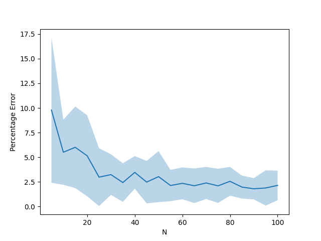
(a)

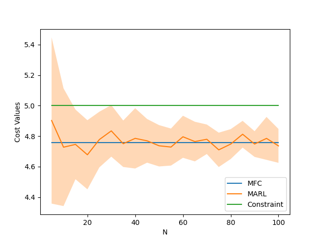
(b)

Figure 1: Fig. (1(a)) portrays the percentage error (defined by $(\ref{eq_error})$) as a function of $N$. On the other hand, Fig. (1(b)) plots the $N$-agent (orange), and infinite-agent (blue) cost-values corresponding to the optimal mean-field policy as a function of $N$. It also shows that both of these values lie below the specified upper bound, $\zeta$ (green). The values of different system parameters are given as: $\alpha_{R}=1$, $\beta_{R}=0.5$, $\lambda_{R}=0.5$, $\lambda_{C}=1$, $\zeta=5$, $\gamma=0.9$, and $Q=10$. The hyperparameters used in Algorithm 1 are chosen as follows: $\eta_{1}=\eta_{2}=\alpha=10^{-3}$, $J=L=10^{2}$. The bold lines, and the half-width of the shaded regions respectively denote the mean-values, and the standard deviation values obtained over $25$ random seeds. The experiments were performed on a $1.8$ GHz Dual-Core Intel $i5$ processor with $8$ GB $1600$ MHz DDR3 memory.

9 Conclusions

This paper shows that a constrained multi-agent reinforcement learning (CMARL) problem can be well-approximated via a constrained mean-field control (CMFC) problem with suitably adjusted constraint bound. We have characterized the approximation error as a function of population size, and the sizes of state, and action spaces respectively. We also state an algorithm to solve the CMFC problem and analyze its sample complexity. One limitation of this study is that it only considers constraints of the form of time-discounted cumulative costs. Studying the same problem with other form of constraints such as, instantaneous cost, average cost etc. could be a potential future direction.

Appendix A Proof of Corollary 2

Using Lemma 3, we obtain,

$$V_{N}^{C}(\boldsymbol{x}_{0}^{N},\boldsymbol{\pi}_{\infty}^{*})\leq V_{\infty}^{C}(\boldsymbol{\mu}_{0},\boldsymbol{\pi}_{\infty}^{*})+G_{C}\overset{(a)}{\leq}0$$

Inequality (a) follows from the fact that $\boldsymbol{\pi}^{*}_{\infty}$ is a feasible solution of (G-CMFC) with $\zeta=-G_{C}$. Clearly, $\boldsymbol{\pi}^{*}_{\infty}$ is a feasible solution of (CMARL). Therefore,

$$V_{N}^{R}(\boldsymbol{x}_{0}^{N},\boldsymbol{\pi}_{N}^{*})-V_{N}^{R}(\boldsymbol{x}_{0}^{N},\boldsymbol{\pi}^{*}_{\infty})$$

$$=V_{N}^{R}(\boldsymbol{x}^{N}_{0},\boldsymbol{\pi}_{N}^{*})-V_{\infty}^{R}(\boldsymbol{\mu}_{0},\boldsymbol{\pi}_{\infty}^{*})+V_{\infty}^{R}(\boldsymbol{\mu}_{0},\boldsymbol{\pi}_{\infty}^{*})-V_{N}^{R}(\boldsymbol{x}_{0}^{N},\boldsymbol{\pi}^{*}_{\infty})$$

$$\overset{(a)}{\leq}2G_{R}+G_{C}\left[\dfrac{4}{\zeta_{0}}\left(\dfrac{M_{R}}{1-\gamma}\right)\right]$$

Inequality (a) follows from Theorem 1, and Lemma 3. This concludes the result.

Appendix B Proof of Lemma 3

In order to establish Lemma 3, the following results are necessary. We use the notation $\pi_{t}$ to indicate the $t$-th component of the policy sequence, $\boldsymbol{\pi}$. Moreover, the $\boldsymbol{\pi}$-induced empirical $N$-agent state, and action distributions at time $t$ are denoted as $\boldsymbol{\mu}_{t}^{N},\boldsymbol{\nu}_{t}^{N}$ respectively. Their counterparts for infinite agent system are $\boldsymbol{\mu}_{t}^{\infty}$, and $\boldsymbol{\nu}_{t}^{\infty}$. Following the notation of section 2, the ($\boldsymbol{\pi}$-induced) joint state, and action at time $t$ are denoted as $\boldsymbol{x}_{t}^{N}\triangleq\{x_{t}^{i}\}_{i\in\{1,\cdots,N\}},\boldsymbol{u}_{t}^{N}\triangleq\{u_{t}^{i}\}_{i\in\{1,\cdots,N\}}$ respectively.

B.1 Lipschitz Continuity Lemmas

Lemma 6

If $\nu^{\mathrm{MF}}(\cdot,\cdot)$ is defined by $(\ref{eq:nu_t})$, then the following holds $\forall t\in\{0,1,\cdots\}$.

$$|\nu^{\mathrm{MF}}(\boldsymbol{\mu}_{t}^{N},\pi_{t})-\nu^{\mathrm{MF}}(\boldsymbol{\mu}_{t}^{\infty},\pi_{t})|_{1}\leq(1+L_{Q})|\boldsymbol{\mu}_{t}^{N}-\boldsymbol{\mu}_{t}^{\infty}|_{1}$$ (37)

Lemma 7

If $P^{\mathrm{MF}}(\cdot,\cdot)$ is defined by $(\ref{eq:mu_t_1})$, then the following holds $\forall t\in\{0,1,\cdots\}$.

$$|P^{\mathrm{MF}}(\boldsymbol{\mu}_{t}^{N},\pi_{t})-P^{\mathrm{MF}}(\boldsymbol{\mu}_{t}^{\infty},\pi_{t})|_{1}\leq S_{P}|\boldsymbol{\mu}-\boldsymbol{\bar{\mu}}|_{1}$$ (38)

where $S_{P}\triangleq 1+2L_{P}+L_{Q}(1+L_{P})$.

Lemma 8

If $r^{\mathrm{MF}}(\cdot,\cdot)$ is defined by $(\ref{eq:r_MF})$, then the following holds $\forall t\in\{0,1,\cdots\}$.

$$|r^{\mathrm{MF}}(\boldsymbol{\mu}_{t}^{N},\pi_{t})-r^{\mathrm{MF}}(\boldsymbol{\mu}_{t}^{\infty},\pi_{t})|\leq S_{R}|\boldsymbol{\mu}_{t}^{N}-\boldsymbol{\mu}_{t}^{\infty}|_{1}$$ (39)

where $S_{R}\triangleq M_{R}+2L_{R}+L_{Q}(M_{R}+L_{R})$.

Lemma 9

If $c^{\mathrm{MF}}(\cdot,\cdot)$ is defined by $(\ref{eq:c_MF})$, then the following holds $\forall t\in\{0,1,\cdots\}$.

$$|c^{\mathrm{MF}}(\boldsymbol{\mu}_{t}^{N},\pi_{t})-c^{\mathrm{MF}}(\boldsymbol{\mu}_{t}^{\infty},\pi_{t})|\leq S_{C}|\boldsymbol{\mu}_{t}^{N}-\boldsymbol{\mu}_{t}^{\infty}|_{1}$$ (40)

where $S_{C}\triangleq M_{C}+2L_{C}+L_{Q}(M_{C}+L_{C})$.

Lemma $\ref{lemma_1}-\ref{lemma_3c}$ shows that the state and action evolution functions, average reward, and cost functions of an infinite agent system are Lipschitz continuous with respect to the state distribution argument. Lemma 6 is an essential ingredient in the proof of Lemma 7, and 8. The proofs of Lemma 6, 7, and 8 are presented in Appendix D, E, and F respectively. The proof of Lemma 9 is identical to that of Lemma 8.

B.2 Large-$N$ Approximation Lemmas

Lemma 10

The following inequality holds $\forall t\in\{0,1,\cdots\}$.

$$\mathbb{E}\big{|}\boldsymbol{\nu}^{N}_{t}-\nu^{\mathrm{MF}}(\boldsymbol{\mu}_{t}^{N},\pi_{t})\big{|}_{1}\leq\dfrac{1}{\sqrt{N}}\sqrt{|\mathcal{U}|}$$

Lemma 11

The following inequality holds $\forall t\in\{0,1,\cdots\}$.

$$\mathbb{E}\left|\boldsymbol{\mu}^{N}_{t+1}-P^{\mathrm{MF}}(\boldsymbol{\mu}^{N}_{t},\pi_{t})\right|_{1}\leq\dfrac{C_{P}}{\sqrt{N}}\left[\sqrt{|\mathcal{X}|}+\sqrt{|\mathcal{U}|}\right]$$

where $C_{P}\triangleq 2+L_{P}$.

Lemma 12

The following inequality holds $\forall t\in\{0,1,\cdots\}$.

$$\mathbb{E}\left|\dfrac{1}{N}\sum_{i=1}r(x_{t}^{i},u_{t}^{i},\boldsymbol{\mu}_{t}^{N},\boldsymbol{\nu}_{t}^{N})-r^{\mathrm{MF}}(\boldsymbol{\mu}_{t}^{N},\pi_{t})\right|\leq\dfrac{M_{R}}{\sqrt{N}}+\dfrac{L_{R}}{\sqrt{N}}\sqrt{|\mathcal{U}|}$$

Lemma 13

The following inequality holds $\forall t\in\{0,1,\cdots\}$.

$$\mathbb{E}\left|\dfrac{1}{N}\sum_{i=1}c(x_{t}^{i},u_{t}^{i},\boldsymbol{\mu}_{t}^{N},\boldsymbol{\nu}_{t}^{N})-c^{\mathrm{MF}}(\boldsymbol{\mu}_{t}^{N},\pi_{t})\right|\leq\dfrac{M_{C}}{\sqrt{N}}+\dfrac{L_{C}}{\sqrt{N}}\sqrt{|\mathcal{U}|}$$

The proofs of Lemma 10, 11, and 12 are given in Appendix G, H, and I, respectively. The proof of Lemma 13 can be obtained by replacing $r,M_{R},L_{R}$ with $c,M_{C},L_{C}$ respectively in the proof of Lemma 12. Finally, invoking Lemma 7, and 11, we obtain the following.

Lemma 14

The following inequality holds $\forall t\in\{0,1,\cdots\}$.

$$\mathbb{E}|\boldsymbol{\mu}_{t}^{N}-\boldsymbol{\mu}_{t}^{\infty}|\leq\dfrac{C_{P}}{\sqrt{N}}\left[\sqrt{|\mathcal{X}|}+\sqrt{|\mathcal{U}|}\right]\left(\dfrac{S_{P}^{t}-1}{S_{P}-1}\right)$$

where $S_{P}$ is defined in Lemma 7 while $C_{P}$ is given in Lemma 11.

The proof of Lemma 14 is given in Appendix J.

B.3 Proof of the Lemma

We shall establish $(\ref{eq_19})$ only for $J=R$. The proof for $J=C$ is identical. Consider the following difference,

$$|V_{N}^{R}(\boldsymbol{x}_{0}^{N},\boldsymbol{\pi})-V_{\infty}^{R}(\boldsymbol{\mu}_{0},\boldsymbol{\pi})|$$

$$\overset{(a)}{\leq}\sum_{t=0}^{\infty}\gamma^{t}\left|\dfrac{1}{N}\sum_{i=1}^{N}\mathbb{E}\left[r(x_{t}^{i},u_{t}^{i},\boldsymbol{\mu}_{t}^{N},\boldsymbol{\nu}_{t}^{N})\right]-r^{\mathrm{MF}}(\boldsymbol{\mu}_{t}^{\infty},\pi_{t})\right|$$

$$\leq\underbrace{\sum_{t=0}^{\infty}\gamma^{t}\mathbb{E}\left|\dfrac{1}{N}r(x_{t}^{i},u_{t}^{i},\boldsymbol{\mu}_{t}^{N},\boldsymbol{\nu}_{t}^{N})-r^{\mathrm{MF}}(\boldsymbol{\mu}_{t}^{N},\pi_{t})\right|}_{\triangleq J_{1}}+\underbrace{\sum_{t=0}^{\infty}\gamma^{t}\mathbb{E}\left|r^{\mathrm{MF}}(\boldsymbol{\mu}_{t}^{N},\pi_{t})-r^{\mathrm{MF}}(\boldsymbol{\mu}_{t}^{\infty},\pi_{t})\right|}_{\triangleq J_{2}}$$

Inequality (a) follows from the definition of the functions $V_{N}^{R}(\cdot,\cdot)$, $V_{\infty}^{R}(\cdot,\cdot)$ given in $(\ref{eq_def_v_r})$, and $(\ref{eq:v_r_mf})$ respectively. The first term, $J_{1}$ can be bounded using Lemma 12 as follows.

$$J_{1}\leq\left(\dfrac{1}{1-\gamma}\right)\left[\dfrac{M_{R}}{\sqrt{N}}+\dfrac{L_{R}}{\sqrt{N}}\sqrt{|\mathcal{U}|}\right]$$

The second term, $J_{2}$, can be bounded as follows.

$$J_{2} \triangleq\sum_{t=0}^{\infty}\gamma^{t}\mathbb{E}|r^{\mathrm{MF}}(\boldsymbol{\mu}_{t}^{N},\pi_{t})-r^{\mathrm{MF}}(\boldsymbol{\mu}_{t}^{\infty},\pi_{t})|$$

$$\overset{(a)}{\leq}S_{R}\sum_{t=0}^{\infty}\gamma^{t}\mathbb{E}|\boldsymbol{\mu}_{t}^{N}-\boldsymbol{\mu}_{t}^{\infty}|$$

$$\overset{(b)}{\leq}\dfrac{1}{\sqrt{N}}\left[\sqrt{|\mathcal{X}|}+\sqrt{|\mathcal{U}|}\right]\left(\dfrac{S_{R}C_{P}}{S_{P}-1}\right)\left[\dfrac{1}{1-\gamma S_{P}}-\dfrac{1}{1-\gamma}\right]$$

Inequality (a) follows from Lemma 8, whereas (b) is a consequence of Lemma 14.

Appendix C Proof of Theorem 4

The proof of Theorem 4 hinges on the following Lemma.

Lemma 15

Let $\boldsymbol{x}_{0}^{N}$ be the initial joint state in an $N$-agent system, and $\boldsymbol{\mu}_{0}$ its empirical distribution. If Assumption $\ref{assumption_1}-\ref{assumption_2}$ hold, then there exists $N_{0}>0$ such that $\forall N\geq N_{0}$, and $\forall\boldsymbol{\pi}\in\Pi_{\infty}$, the following inequalities hold whenever $\gamma S_{P}<1$.

$$|V_{N}^{J}(\boldsymbol{x}_{0}^{N},\boldsymbol{\pi})-V_{\infty}^{J}(\boldsymbol{\mu}_{0},\boldsymbol{\pi})|\leq G_{J}^{0}$$ (41)

where $J\in\{R,C\}$. The value functions $V_{N}^{R},V_{N}^{C}$ are given by $(\ref{eq_def_v_r}),(\ref{eq_def_v_c})$ respectively, and the terms $G_{R}^{0},G_{C}^{0},S_{P}$ are defined in Theorem 4.

The role Lemma 15 in establishing Theorem 4 is analogous to the role of Lemma 3 in proving Theorem 1. In this section, we shall primarily focus on proving Lemma 15. Once it is established, Theorem 4 can be proven following argument similar to that is used in section 5.

C.1 Auxiliary Lemmas

To prove Lemma 15, the following results are necessary. The notations are same as used in Appendix B.

Lemma 16

The following inequality holds $\forall t\in\{0,1,\cdots\}$.

$$\mathbb{E}\left|\boldsymbol{\mu}^{N}_{t+1}-P^{\mathrm{MF}}(\boldsymbol{\mu}^{N}_{t},\pi_{t})\right|_{1}\leq\dfrac{2}{\sqrt{N}}\sqrt{|\mathcal{X}|}$$ (42)

Lemma 17

The following inequality holds $\forall t\in\{0,1,\cdots\}$.

$$\mathbb{E}\left|\dfrac{1}{N}\sum_{i=1}r(x_{t}^{i},u_{t}^{i},\boldsymbol{\mu}_{t}^{N})-r^{\mathrm{MF}}(\boldsymbol{\mu}_{t}^{N},\pi_{t})\right|\leq\dfrac{M_{R}}{\sqrt{N}}$$

Lemma 18

The following inequality holds $\forall t\in\{0,1,\cdots\}$.

$$\mathbb{E}\left|\dfrac{1}{N}\sum_{i=1}c(x_{t}^{i},u_{t}^{i},\boldsymbol{\mu}_{t}^{N})-c^{\mathrm{MF}}(\boldsymbol{\mu}_{t}^{N},\pi_{t})\right|\leq\dfrac{M_{C}}{\sqrt{N}}$$

Lemma 19

The following inequality holds $\forall t\in\{0,1,\cdots\}$.

$$\mathbb{E}|\boldsymbol{\mu}_{t}^{N}-\boldsymbol{\mu}_{t}^{\infty}|\leq\dfrac{2}{\sqrt{N}}\sqrt{|\mathcal{X}|}\left(\dfrac{S_{P}^{t}-1}{S_{P}-1}\right)$$

The term $S_{P}$ is defined in Lemma 7.

The proofs of Lemma 16, 17, 19 are relegated to Appendix K, L, and M, respectively. The proof of Lemma 18 can be obtained by replacing $r$ with $c$, and $M_{R}$ with $M_{C}$ in the proof of Lemma 17.

C.2 Proof of Lemma 15

We use the same notations as in Appendix B.3. Consider the following difference,

$$|V_{N}^{R}(\boldsymbol{x}_{0}^{N},\boldsymbol{\pi})-V_{\infty}^{R}(\boldsymbol{\mu}_{0},\boldsymbol{\pi})|$$

$$\overset{(a)}{\leq}\sum_{t=0}^{\infty}\gamma^{t}\left|\dfrac{1}{N}\sum_{i=1}^{N}r(x_{t}^{i},u_{t}^{i},\boldsymbol{\mu}_{t}^{N})\right]-\mathbb{E}\left[r^{\mathrm{MF}}(\boldsymbol{\mu}_{t}^{\infty},\pi_{t})\right|$$

$$\leq\underbrace{\sum_{t=0}^{\infty}\gamma^{t}\mathbb{E}\left|\dfrac{1}{N}r(x_{t}^{i},u_{t}^{i},\boldsymbol{\mu}_{t}^{N})-r^{\mathrm{MF}}(\boldsymbol{\mu}_{t}^{N},\pi_{t})\right|}_{\triangleq J_{1}}+\underbrace{\sum_{t=0}^{\infty}\gamma^{t}\mathbb{E}\left|r^{\mathrm{MF}}(\boldsymbol{\mu}_{t}^{N},\pi_{t})-r^{\mathrm{MF}}(\boldsymbol{\mu}_{t}^{\infty},\pi_{t})\right|}_{\triangleq J_{2}}$$

Inequality (a) follows from the definition of the value functions $V_{N}^{R}(\cdot,\cdot)$, $V_{\infty}^{C}(\cdot,\cdot)$ given in $(\ref{eq_def_v_r})$, and $(\ref{eq:v_r_mf})$ respectively. The first term, $J_{1}$ can be bounded using Lemma 12 as follows.

$$J_{1}\leq\dfrac{M_{R}}{\sqrt{N}}\left(\dfrac{1}{1-\gamma}\right)$$

The second term, $J_{2}$, can be bounded as follows.

$$J_{2} \triangleq\sum_{t=0}^{\infty}\gamma^{t}\mathbb{E}|r^{\mathrm{MF}}(\boldsymbol{\mu}_{t}^{N},\pi_{t})-r^{\mathrm{MF}}(\boldsymbol{\mu}_{t}^{\infty},\pi_{t})|$$

$$\overset{(a)}{\leq}S_{R}\sum_{t=0}^{\infty}\gamma^{t}\mathbb{E}|\boldsymbol{\mu}_{t}^{N}-\boldsymbol{\mu}_{t}^{\infty}|$$

$$\overset{(b)}{\leq}\dfrac{1}{\sqrt{N}}\sqrt{|\mathcal{X}|}\left(\dfrac{2S_{R}}{S_{P}-1}\right)\left[\dfrac{1}{1-\gamma S_{P}}-\dfrac{1}{1-\gamma}\right]$$

Inequality (a) follows from Lemma 8, whereas (b) is a consequence of Lemma 19. This establishes $(\ref{eq_19a})$ for $J=R$. The other case, $J=C$, can be proven similarly.

Appendix D Proof of Lemma 6

Note the following inequalities.

$$|\nu^{\mathrm{MF}}(\boldsymbol{\mu}_{t}^{N},\pi_{t})-\nu^{\mathrm{MF}}(\boldsymbol{\mu}_{t}^{\infty},\pi_{t})|_{1}$$

$$\overset{(a)}{=}\Bigg{|}\sum_{x\in\mathcal{X}}\pi_{t}(x,\boldsymbol{\mu}_{t}^{N})\boldsymbol{\mu}_{t}^{N}(x)-\sum_{x\in\mathcal{X}}\pi_{t}(x,\boldsymbol{\mu}_{t}^{\infty})\boldsymbol{\mu}_{t}^{\infty}(x)\Bigg{|}_{1}$$

$$=\sum_{u\in\mathcal{U}}\Bigg{|}\sum_{x\in\mathcal{X}}\pi_{t}(x,\boldsymbol{\mu}_{t}^{N})(u)\boldsymbol{\mu}_{t}^{N}(x)-\sum_{x\in\mathcal{X}}\pi_{t}(x,\boldsymbol{\mu}_{t}^{\infty})(u)\boldsymbol{\mu}_{t}^{\infty}(x)\Bigg{|}$$

$$\leq\sum_{x\in\mathcal{X}}\sum_{u\in\mathcal{U}}|\pi_{t}(x,\boldsymbol{\mu}_{t}^{N})(u)\boldsymbol{\mu}_{t}^{N}(x)-\pi_{t}(x,\boldsymbol{\mu}_{t}^{\infty})(u)\boldsymbol{\mu}_{t}^{\infty}(x)|$$

$$\leq\sum_{x\in\mathcal{X}}|\boldsymbol{\mu}_{t}^{N}(x)-\boldsymbol{\mu}_{t}^{\infty}(x)|\underbrace{\sum_{u\in\mathcal{U}}\pi_{t}(x,\boldsymbol{\mu}_{t}^{N})(u)}_{=1}+\sum_{x\in\mathcal{X}}\boldsymbol{\mu}_{t}^{\infty}(x)\sum_{u\in\mathcal{U}}|\pi_{t}(x,\boldsymbol{\mu}_{t}^{N})(u)-\pi_{t}(x,\boldsymbol{\mu}_{t}^{\infty})(u)|$$

$$\overset{(b)}{\leq}|\boldsymbol{\mu}_{t}^{N}-\boldsymbol{\mu}_{t}^{\infty}|_{1}+L_{Q}|\boldsymbol{\mu}_{t}^{N}-\boldsymbol{\mu}_{t}^{\infty}|\underbrace{\sum_{x\in\mathcal{X}}\boldsymbol{\mu}_{t}^{\infty}(x)}_{=1}$$

$$\overset{(c)}{=}(1+L_{Q})|\boldsymbol{\mu}_{t}^{N}-\boldsymbol{\mu}_{t}^{\infty}|_{1}$$

Equality (a) follows from the definition of $\nu^{\mathrm{MF}}(\cdot,\cdot)$ as given in $(\ref{eq:nu_t})$. On the other hand, inequality (b) is a consequence of Assumption 2, and the fact that $\pi_{t}(x,\boldsymbol{\mu}_{t}^{N})$ is probability distribution $\forall x\in\mathcal{X}$. Finally, (c) follows because $\boldsymbol{\mu}_{t}^{\infty}$ is a probability distribution. This concludes the result.

Appendix E Proof of Lemma 7

Note that,

$$|P^{\mathrm{MF}}(\boldsymbol{\mu}_{t}^{N},\pi_{t})-P^{\mathrm{MF}}(\boldsymbol{\mu}_{t}^{\infty},\pi_{t})|_{1}$$

$$\overset{(a)}{=}\Bigg{|}\sum_{x\in\mathcal{X}}\sum_{u\in\mathcal{U}}P(x,u,\boldsymbol{\mu}_{t}^{N},\nu^{\mathrm{MF}}(\boldsymbol{\mu}_{t}^{N},\pi_{t}))\pi_{t}(x,\boldsymbol{\mu}_{t}^{N})(u)\boldsymbol{\mu}_{t}^{N}(x)-P(x,u,\boldsymbol{\mu}_{t}^{\infty},\nu^{\mathrm{MF}}(\boldsymbol{\mu}_{t}^{\infty},\pi_{t}))\pi_{t}(x,\boldsymbol{\mu}_{t}^{\infty})(u)\boldsymbol{\mu}_{t}^{\infty}(x)\Bigg{|}_{1}$$

$$\leq J_{1}+J_{2}$$

Equality (a) follows from the definition of $P^{\mathrm{MF}}(\cdot,\cdot)$ as stated in $(\ref{eq:mu_t_1})$. The first term can be bounded as follows.

$$J_{1}\triangleq \sum_{x\in\mathcal{X}}\sum_{u\in\mathcal{U}}\Big{|}P(x,u,\boldsymbol{\mu}_{t}^{N},\nu^{\mathrm{MF}}(\boldsymbol{\mu}_{t}^{N},\pi_{t}))-P(x,u,\boldsymbol{\mu}_{t}^{\infty},\nu^{\mathrm{MF}}(\boldsymbol{\mu}_{t}^{\infty},\pi_{t}))\Big{|}_{1}\times\pi_{t}(x,\boldsymbol{\mu}_{t}^{N})(u)\boldsymbol{\mu}_{t}^{N}(x)$$

$$\overset{(a)}{\leq}L_{P}\left[|\boldsymbol{\mu}_{t}^{N}-\boldsymbol{\mu}_{t}^{\infty}|_{1}+|\nu^{\mathrm{MF}}(\boldsymbol{\mu}_{t}^{N},\pi_{t})-\nu^{\mathrm{MF}}(\boldsymbol{\mu}_{t}^{\infty},\pi_{t})|_{1}\right]\times\underbrace{\sum_{x\in\mathcal{X}}\boldsymbol{\mu}_{t}^{N}(x)\sum_{u\in\mathcal{U}}\pi_{t}(x,\boldsymbol{\mu}_{t}^{N})(u)}_{=1}$$

$$\overset{(b)}{\leq}L_{P}(2+L_{Q})|\boldsymbol{\mu}_{t}^{N}-\boldsymbol{\mu}_{t}^{\infty}|_{1}$$

Inequality $(a)$ is a result of Assumption 1(e) while $(b)$ follows from Lemma 6, and the fact that $\pi_{t}(x,\boldsymbol{\mu}_{t}^{N})$, $\boldsymbol{\mu}_{t}^{N}$ are probability distributions $\forall x\in\mathcal{X}$. The second term, $J_{2}$ can be bounded as follows.

$$J_{2}\triangleq \sum_{x\in\mathcal{X}}\sum_{u\in\mathcal{U}}\underbrace{|P(x,u,\boldsymbol{\mu}_{t}^{\infty},\nu^{\mathrm{MF}}(\boldsymbol{\mu}_{t}^{\infty},\pi_{t}))|_{1}}_{=1}\times|\pi_{t}(x,\boldsymbol{\mu}_{t}^{N})(u)\boldsymbol{\mu}_{t}^{N}(x)-\pi_{t}(x,\boldsymbol{\mu}_{t}^{\infty})(u)\boldsymbol{\mu}_{t}^{\infty}(x)|$$

$$\leq\sum_{x\in\mathcal{X}}|\boldsymbol{\mu}_{t}^{N}(x)-\boldsymbol{\mu}_{t}^{\infty}(x)|\underbrace{\sum_{u\in\mathcal{U}}\pi_{t}(x,\boldsymbol{\mu}_{t}^{N})(u)}_{=1}+\sum_{x\in\mathcal{X}}\boldsymbol{\mu}_{t}^{\infty}(x)\sum_{u\in\mathcal{U}}|\pi_{t}(x,\boldsymbol{\mu}_{t}^{N})(u)-\pi_{t}(x,\boldsymbol{\mu}_{t}^{\infty})(u)|$$

$$\overset{(a)}{\leq}|\boldsymbol{\mu}_{t}^{N}-\boldsymbol{\mu}_{t}^{\infty}|_{1}+L_{P}|\boldsymbol{\mu}_{t}^{N}-\boldsymbol{\mu}_{t}^{\infty}|_{1}\underbrace{\sum_{x\in\mathcal{X}}\boldsymbol{\mu}_{t}^{\infty}(x)}_{=1}$$

$$=(1+L_{P})|\boldsymbol{\mu}_{t}^{N}-\boldsymbol{\mu}_{t}^{\infty}|_{1}$$

Inequality $(a)$ follows from the fact that $\pi_{t}(x,\boldsymbol{\mu}_{t}^{N})$ is a probability distribution $\forall x\in\mathcal{X}$ while $(b)$ uses Assumption 2, and the fact that $\boldsymbol{\mu}_{t}^{\infty}$ is a probability distribution. This concludes the result.

Appendix F Proof of Lemma 8

Notice the following inequality,

$$|r^{\mathrm{MF}}(\boldsymbol{\mu}_{t}^{N},\pi_{t})-r^{\mathrm{MF}}(\boldsymbol{\mu}_{t}^{\infty},\pi_{t})|$$

$$\overset{(a)}{=}\Bigg{|}\sum_{x\in\mathcal{X}}\sum_{u\in\mathcal{U}}r(x,u,\boldsymbol{\mu}_{t}^{N},\nu^{\mathrm{MF}}(\boldsymbol{\mu}_{t}^{N},\pi_{t}))\pi_{t}(x,\boldsymbol{\mu}_{t}^{N})(u)\boldsymbol{\mu}_{t}^{N}(x)-r(x,u,\boldsymbol{\mu}_{t}^{\infty},\nu^{\mathrm{MF}}(\boldsymbol{\mu}_{t}^{\infty},\pi_{t}))\pi_{t}(x,\boldsymbol{\mu}_{t}^{\infty})(u)\boldsymbol{\mu}_{t}^{\infty}(x)\Bigg{|}$$

$$\leq J_{1}+J_{2}$$

Equality (a) follows from the definition of $r^{\mathrm{MF}}(\cdot,\cdot)$ as depicted in $(\ref{eq:r_MF})$. The first term can be bounded as follows.

$$J_{1}\triangleq \sum_{x\in\mathcal{X}}\sum_{u\in\mathcal{U}}\Big{|}r(x,u,\boldsymbol{\mu}_{t}^{N},\nu^{\mathrm{MF}}(\boldsymbol{\mu}_{t}^{N},\pi_{t}))-r(x,u,\boldsymbol{\mu}_{t}^{\infty},\nu^{\mathrm{MF}}(\boldsymbol{\mu}_{t}^{\infty},\pi_{t}))\Big{|}\times\pi_{t}(x,\boldsymbol{\mu}_{t}^{N})(u)\boldsymbol{\mu}_{t}^{N}(x)$$

$$\overset{(a)}{\leq}L_{R}\left[|\boldsymbol{\mu}_{t}^{N}-\boldsymbol{\mu}_{t}^{\infty}|_{1}+|\nu^{\mathrm{MF}}(\boldsymbol{\mu}_{t}^{N},\pi_{t})-\nu^{\mathrm{MF}}(\boldsymbol{\mu}_{t}^{\infty},\pi_{t})|_{1}\right]\times\underbrace{\sum_{x\in\mathcal{X}}\boldsymbol{\mu}_{t}^{N}(x)\sum_{u\in\mathcal{U}}\pi_{t}(x,\boldsymbol{\mu}_{t}^{N})(u)}_{=1}$$

$$\overset{(b)}{\leq}L_{R}(2+L_{Q})|\boldsymbol{\mu}_{t}^{N}-\boldsymbol{\mu}_{t}^{\infty}|_{1}$$

Inequality $(a)$ is a result of Assumption 1(c) while relation $(b)$ follows from Lemma 6, and the fact that $\pi_{t}(x,\boldsymbol{\mu}_{t}^{\infty})$, $\boldsymbol{\mu}_{t}^{N}$ are probability distributions $\forall x\in\mathcal{X}$. The term, $J_{2}$ can be bounded as follows.

$$J_{2}\triangleq \sum_{x\in\mathcal{X}}\sum_{u\in\mathcal{U}}|r(x,u,\boldsymbol{\mu}_{t}^{\infty},\nu^{\mathrm{MF}}(\boldsymbol{\mu}_{t}^{\infty},\pi_{t}))|\times|\pi_{t}(x,\boldsymbol{\mu}_{t}^{N})(u)\boldsymbol{\mu}_{t}^{N}(x)-\pi_{t}(x,\boldsymbol{\mu}_{t}^{\infty})(u)\boldsymbol{\mu}_{t}^{\infty}(x)|$$

$$\overset{(a)}{\leq}M_{R}\sum_{x\in\mathcal{X}}\sum_{u\in\mathcal{U}}|\pi_{t}(x,\boldsymbol{\mu}_{t}^{N})(u)\boldsymbol{\mu}_{t}^{N}(x)-\pi_{t}(x,\boldsymbol{\mu}_{t}^{\infty})(u)\boldsymbol{\mu}_{t}^{\infty}(x)|$$

$$\leq M_{R}\sum_{x\in\mathcal{X}}|\boldsymbol{\mu}_{t}^{N}(x)-\boldsymbol{\mu}_{t}^{\infty}(x)|\underbrace{\sum_{u\in\mathcal{U}}\pi_{t}(x,\boldsymbol{\mu}_{t}^{N})(u)}_{=1}+M_{R}\sum_{x\in\mathcal{X}}\boldsymbol{\mu}_{t}^{\infty}(x)\sum_{u\in\mathcal{U}}|\pi_{t}(x,\boldsymbol{\mu}_{t}^{N})(u)-\pi_{t}(x,\boldsymbol{\mu}_{t}^{\infty})(u)|$$

$$\overset{(b)}{\leq}M_{R}|\boldsymbol{\mu}_{t}^{N}-\boldsymbol{\mu}_{t}^{\infty}|_{1}+M_{R}L_{Q}|\boldsymbol{\mu}_{t}^{N}-\boldsymbol{\mu}_{t}^{\infty}|_{1}\underbrace{\sum_{x\in\mathcal{X}}\boldsymbol{\mu}_{t}^{\infty}(x)}_{=1}\overset{(c)}{=}M_{R}(1+L_{Q})|\boldsymbol{\mu}_{t}^{N}-\boldsymbol{\mu}_{t}^{\infty}|_{1}$$

Inequality $(a)$ follows from Assumption 1(a). On the other hand, $(b)$ is a consequence of Assumption 2. Finally, (c) follows from the fact that $\boldsymbol{\mu}_{t}^{\infty}$ is a probability distribution. This concludes the result.

Appendix G Proof of Lemma 10

The following Lemma is required to prove the result.

Lemma 20

If $\forall m\in\{1,\cdots,M\}$, $\{X_{mn}\}_{n\in\{1,\cdots,N\}}$ are independent random variables that lie in $[0,1]$, and satisfy $\sum_{m\in\{1,\cdots,M\}}\mathbb{E}[X_{mn}]\leq 1$, $\forall n\in\{1,\cdots,N\}$, then the following holds,

$$\sum_{m=1}^{M}\mathbb{E}\left|\sum_{n=1}^{N}\left(X_{mn}-\mathbb{E}[X_{mn}]\right)\right|\leq\sqrt{MN}$$ (43)

Lemma 20 is adapted from Lemma 13 of (Mondal et al., 2022a).

Observe the following inequalities.

$$\mathbb{E}\left|\boldsymbol{\nu}_{t}^{N}-\nu^{\mathrm{MF}}(\boldsymbol{\mu}_{t}^{N},\pi_{t})\right|_{1}$$

$$=\mathbb{E}\left[\mathbb{E}\left[\left|\boldsymbol{\nu}^{N}_{t}-\nu^{\mathrm{MF}}(\boldsymbol{\mu}^{N}_{t},\pi_{t})\right|_{1}\Big{|}\boldsymbol{x}_{t}^{N}\right]\right]$$

$$\overset{(a)}{=}\mathbb{E}\left[\mathbb{E}\left[\left|\boldsymbol{\nu}_{t}^{N}-\sum_{x\in\mathcal{X}}\pi_{t}(x,\boldsymbol{\mu}_{t}^{N})\boldsymbol{\mu}_{t}^{N}(x)\right|_{1}\Bigg{|}\boldsymbol{x}_{t}^{N}\right]\right]$$

$$=\mathbb{E}\left[\mathbb{E}\left[\sum_{u\in\mathcal{U}}\left|\boldsymbol{\nu}^{N}_{t}(u)-\sum_{x\in\mathcal{X}}\pi_{t}(x,\boldsymbol{\mu}_{t}^{N})(u)\boldsymbol{\mu}^{N}_{t}(x)\right|\Bigg{|}\boldsymbol{x}_{t}^{N}\right]\right]$$

$$\overset{(b)}{=}\mathbb{E}\left[\sum_{u\in\mathcal{U}}\mathbb{E}\left[\dfrac{1}{N}\left|\sum_{i=1}^{N}\delta(u_{t}^{i}=u)-\dfrac{1}{N}\sum_{x\in\mathcal{X}}\pi_{t}(x,\boldsymbol{\mu}_{t}^{N})(u)\sum_{i=1}^{N}\delta(x_{t}^{i}=x)\right|\Bigg{|}\boldsymbol{x}_{t}^{N}\right]\right]$$

$$=\mathbb{E}\left[\sum_{u\in\mathcal{U}}\mathbb{E}\left[\left|\dfrac{1}{N}\sum_{i=1}^{N}\delta(u_{t}^{i}=u)-\dfrac{1}{N}\sum_{i=1}^{N}\pi_{t}(x_{t}^{i},\boldsymbol{\mu}_{t}^{N})(u)\right|\Bigg{|}\boldsymbol{x}_{t}^{N}\right]\right]$$

$$\overset{(c)}{\leq}\dfrac{1}{\sqrt{N}}\sqrt{|\mathcal{U}|}$$

Equality (a) follows from the definition of $\nu^{\mathrm{MF}}(\cdot,\cdot)$ as depicted in $(\ref{eq:nu_t})$ while (b) is a consequence of the definitions of $\boldsymbol{\mu}_{t}^{N},\boldsymbol{\nu}_{t}^{N}$. Finally, (c) is an application of Lemma 20. Specifically, it uses the facts that, $\{u_{t}^{i}\}_{i\in\{1,\cdots,N\}}$ are conditionally independent given $\boldsymbol{x}_{t}^{N}$, and

$$\mathbb{E}\left[\delta(u_{t}^{i}=u)\Big{|}\boldsymbol{x}_{t}^{N}\right]=\pi_{t}(x_{t}^{i},\boldsymbol{\mu}_{t}^{N})(u),$$

$$\sum_{u\in\mathcal{U}}\mathbb{E}\left[\delta(u_{t}^{i}=u)\Big{|}\boldsymbol{x}_{t}^{N}\right]=1$$

$~{}\forall i\in\{1,\cdots,N\},\forall u\in\mathcal{U}$. This concludes the lemma.

Appendix H Proof of Lemma 11

Note that,

$$\mathbb{E}\left|\boldsymbol{\mu}_{t+1}^{N}-P^{\mathrm{MF}}(\boldsymbol{\mu}^{N}_{t},\pi_{t})\right|_{1}$$

$$\overset{(a)}{=}\sum_{x\in\mathcal{X}}\mathbb{E}\left|\dfrac{1}{N}\sum_{i=1}^{N}\delta(x_{t+1}^{i}=x)-\sum_{x^{\prime}\in\mathcal{X}}\sum_{u\in\mathcal{U}}P(x^{\prime},u,\boldsymbol{\mu}^{N}_{t},\nu^{\mathrm{MF}}(\boldsymbol{\mu}^{N}_{t},\pi_{t}))(x)\pi_{t}(x^{\prime},\boldsymbol{\mu}_{t}^{N})(u)\dfrac{1}{N}\sum_{i=1}^{N}\delta(x_{t}^{i}=x^{\prime})\right|$$

$$=\sum_{x\in\mathcal{X}}\mathbb{E}\left|\dfrac{1}{N}\sum_{i=1}^{N}\delta(x_{t+1}^{i}=x)-\dfrac{1}{N}\sum_{i=1}^{N}\sum_{u\in\mathcal{U}}P(x_{t}^{i},u,\boldsymbol{\mu}^{N}_{t},\nu^{\mathrm{MF}}(\boldsymbol{\mu}^{N}_{t},\pi_{t}))(x)\pi_{t}(x_{t}^{i},\boldsymbol{\mu}_{t}^{N})(u)\right|$$

$$\leq J_{1}+J_{2}+J_{3}$$

Equality (a) follows from the definition of $P^{\mathrm{MF}}(\cdot,\cdot)$ as given in $(\ref{eq:mu_t_1})$. The first term, $J_{1}$, can be upper bounded as follows.

$$J_{1} \triangleq\dfrac{1}{N}\sum_{x\in\mathcal{X}}\mathbb{E}\left|\sum_{i=1}^{N}\delta(x_{t+1}^{i}=x)-\sum_{i=1}^{N}P(x_{t}^{i},u_{t}^{i},\boldsymbol{\mu}^{N}_{t},\boldsymbol{\nu}_{t}^{N})(x)\right|$$

$$=\dfrac{1}{N}\sum_{x\in\mathcal{X}}\mathbb{E}\left[\mathbb{E}\left[\left|\sum_{i=1}^{N}\delta(x_{t+1}^{i}=x)-\sum_{i=1}^{N}P(x_{t}^{i},u_{t}^{i},\boldsymbol{\mu}^{N}_{t},\boldsymbol{\nu}_{t}^{N})(x)\right|\Bigg{|}\boldsymbol{x}_{t}^{N},\boldsymbol{u}_{t}^{N}\right]\right]$$

$$\overset{(a)}{\leq}\dfrac{1}{\sqrt{N}}\sqrt{|\mathcal{X}|}$$

Inequality $(a)$ can be derived using Lemma 20, and the facts that $\{x_{t+1}^{i}\}_{i\in\{1,\cdots,N\}}$ are conditionally independent given $\{\boldsymbol{x}_{t}^{N},\boldsymbol{u}_{t}^{N}\}$, and,

$$\mathbb{E}\left[\delta(x_{t+1}^{i}=x)\Big{|}\boldsymbol{x}_{t}^{N},\boldsymbol{u}_{t}^{N}\right]=P(x_{t}^{i},u_{t}^{i},\boldsymbol{\mu}^{N}_{t},\boldsymbol{\nu}_{t}^{N})(x),$$

$$\sum_{x\in\mathcal{X}}\mathbb{E}\left[\delta(x_{t+1}^{i}=x)\Big{|}\boldsymbol{x}_{t}^{N},\boldsymbol{u}_{t}^{N}\right]=1$$

$\forall i\in\{1,\cdots,N\}$, and $\forall x\in\mathcal{X}$. The second term can be upper bounded as follows.

$$J_{2} \triangleq\dfrac{1}{N}\sum_{x\in\mathcal{X}}\mathbb{E}\left|\sum_{i=1}^{N}P(x_{t}^{i},u_{t}^{i},\boldsymbol{\mu}_{t}^{N},\boldsymbol{\nu}_{t}^{N})(x)-\sum_{i=1}^{N}P(x_{t}^{i},u_{t}^{i},\boldsymbol{\mu}^{N}_{t},\nu^{\mathrm{MF}}(\boldsymbol{\mu}^{N}_{t},\pi_{t}))(x)\right|$$

$$\leq\dfrac{1}{N}\sum_{i=1}^{N}\mathbb{E}\left|P(x_{t}^{i},u_{t}^{i},\boldsymbol{\mu}_{t}^{N},\boldsymbol{\nu}_{t}^{N})-P(x_{t}^{i},u_{t}^{i},\boldsymbol{\mu}^{N}_{t},\nu^{\mathrm{MF}}(\boldsymbol{\mu}^{N}_{t},\pi_{t}))\right|_{1}$$

$$\overset{(a)}{\leq}L_{P}\mathbb{E}\left|\boldsymbol{\nu}_{t}^{N}-\nu^{\mathrm{MF}}(\boldsymbol{\mu}_{t}^{N},\pi_{t})\right|_{1}\overset{(b)}{\leq}\dfrac{L_{P}}{\sqrt{N}}\sqrt{|\mathcal{U}|}$$

Inequality (a) follows from Assumption 3 while (b) follows from Lemma 10. Finally, the third term can be bounded as follows.

$$J_{3} \triangleq\dfrac{1}{N}\sum_{x\in\mathcal{X}}\mathbb{E}\left|\sum_{i=1}^{N}P(x_{t}^{i},u_{t}^{i},\boldsymbol{\mu}^{N}_{t},\nu^{\mathrm{MF}}(\boldsymbol{\mu}^{N}_{t},\pi_{t}))(x)-\sum_{i=1}^{N}\sum_{u\in\mathcal{U}}P(x_{t}^{i},u,\boldsymbol{\mu}^{N}_{t},\nu^{\mathrm{MF}}(\boldsymbol{\mu}^{N}_{t},\pi_{t}))(x)\pi_{t}(x_{t}^{i},\boldsymbol{\mu}_{t}^{N})(u)\right|$$

$$\overset{(a)}{\leq}\dfrac{1}{\sqrt{N}}\sqrt{|\mathcal{X}|}$$

Inequality (a) is a consequence of Lemma 20. Specifically, it uses the facts that, $\{u_{t}^{i}\}_{i\in\{1,\cdots,N\}}$ are conditionally independent given $\boldsymbol{x}_{t}^{N}$, and

$$\mathbb{E}\left[P(x_{t}^{i},u_{t}^{i},\boldsymbol{\mu}^{N}_{t},\nu^{\mathrm{MF}}(\boldsymbol{\mu}^{N}_{t},\pi_{t}))(x)\Big{|}\boldsymbol{x}_{t}^{N}\right]=\sum_{u\in\mathcal{U}}P(x_{t}^{i},u,\boldsymbol{\mu}^{N}_{t},\nu^{\mathrm{MF}}(\boldsymbol{\mu}^{N}_{t},\pi_{t}))(x)\pi_{t}(x_{t}^{i},\boldsymbol{\mu}_{t}^{N})(u),$$

$$\sum_{x\in\mathcal{X}}\mathbb{E}\left[P(x_{t}^{i},u_{t}^{i},\boldsymbol{\mu}^{N}_{t},\nu^{\mathrm{MF}}(\boldsymbol{\mu}^{N}_{t},\pi_{t}))(x)\Big{|}\boldsymbol{x}_{t}^{N}\right]=1$$

$\forall i\in\{1,\cdots,N\}$, and $\forall x\in\mathcal{X}$. This concludes the Lemma.

Appendix I Proof of Lemma 12

Note that,

$$\mathbb{E}\left|\dfrac{1}{N}\sum_{i=1}r(x_{t}^{i},u_{t}^{i},\boldsymbol{\mu}_{t}^{N},\boldsymbol{\nu}_{t}^{N})-r^{\mathrm{MF}}(\boldsymbol{\mu}_{t}^{N},\pi_{t})\right|$$

$$\overset{(a)}{=}\mathbb{E}\left|\dfrac{1}{N}\sum_{i=1}^{N}r(x_{t}^{i},u_{t}^{i},\boldsymbol{\mu}_{t}^{N},\boldsymbol{\nu}_{t}^{N})-\sum_{x\in\mathcal{X}}\sum_{u\in\mathcal{U}}r(x,u,\boldsymbol{\mu}_{t}^{N},\nu^{\mathrm{MF}}(\boldsymbol{\mu}_{t}^{N},\pi_{t}))\pi_{t}(x,\boldsymbol{\mu}_{t}^{N})(u)\dfrac{1}{N}\sum_{i=1}^{N}\delta(x_{t}^{i}=x)\right|$$

$$=\mathbb{E}\left|\dfrac{1}{N}\sum_{i=1}^{N}r(x_{t}^{i},u_{t}^{i},\boldsymbol{\mu}_{t}^{N},\boldsymbol{\nu}_{t}^{N})-\dfrac{1}{N}\sum_{i=1}^{N}\sum_{u\in\mathcal{U}}r(x_{t}^{i},u,\boldsymbol{\mu}_{t}^{N},\nu^{\mathrm{MF}}(\boldsymbol{\mu}_{t}^{N},\pi_{t}))\pi_{t}(x_{t}^{i},\boldsymbol{\mu}_{t}^{N})(u)\right|$$

$$\leq J_{1}+J_{2}$$

Equation (a) is a result of the definition of $r^{\mathrm{MF}}(\cdot,\cdot)$ as given in $(\ref{eq:r_MF})$. The first term, $J_{1}$, can be bounded as follows.

$$J_{1} \triangleq\dfrac{1}{N}\mathbb{E}\left|\sum_{i=1}^{N}r(x_{t}^{i},u_{t}^{i},\boldsymbol{\mu}_{t}^{N},\boldsymbol{\nu}_{t}^{N})-\sum_{i=1}^{N}r(x_{t}^{i},u_{t}^{i},\boldsymbol{\mu}_{t}^{N},\nu^{\mathrm{MF}}(\boldsymbol{\mu}_{t}^{N},\pi_{t}))\right|$$

$$\leq\dfrac{1}{N}\mathbb{E}\sum_{i=1}^{N}\left|r(x_{t}^{i},u_{t}^{i},\boldsymbol{\mu}_{t}^{N},\boldsymbol{\nu}_{t}^{N})-r(x_{t}^{i},u_{t}^{i},\boldsymbol{\mu}_{t}^{N},\nu^{\mathrm{MF}}(\boldsymbol{\mu}_{t}^{N},\pi_{t}))\right|$$

$$\overset{(a)}{\leq}L_{R}\mathbb{E}\left|\boldsymbol{\nu}_{t}^{N}-\nu^{\mathrm{MF}}(\boldsymbol{\mu}_{t}^{N},\pi_{t})\right|_{1}$$

$$\overset{(b)}{\leq}\dfrac{L_{R}}{\sqrt{N}}\sqrt{|\mathcal{U}|}$$

Inequality (a) follows from Assumption 1, and (b) is a consequence of Lemma 10. The second term, $J_{2}$, can be bounded as follows.

$$J_{2} \triangleq\dfrac{1}{N}\mathbb{E}\left|\sum_{i=1}^{N}r(x_{t}^{i},u_{t}^{i},\boldsymbol{\mu}_{t}^{N},\nu^{\mathrm{MF}}(\boldsymbol{\mu}_{t}^{N},\pi_{t}))-\sum_{i=1}^{N}\sum_{u\in\mathcal{U}}r(x_{t}^{i},u,\boldsymbol{\mu}_{t}^{N},\nu^{\mathrm{MF}}(\boldsymbol{\mu}_{t}^{N},\pi_{t}))\pi_{t}(x_{t}^{i},\boldsymbol{\mu}_{t}^{N})(u)\right|$$

$$=\dfrac{1}{N}\mathbb{E}\left[\mathbb{E}\left[\left|\sum_{i=1}^{N}r(x_{t}^{i},u_{t}^{i},\boldsymbol{\mu}_{t}^{N},\nu^{\mathrm{MF}}(\boldsymbol{\mu}_{t}^{N},\pi_{t}))-\sum_{i=1}^{N}\sum_{u\in\mathcal{U}}r(x_{t}^{i},u,\boldsymbol{\mu}_{t}^{N},\nu^{\mathrm{MF}}(\boldsymbol{\mu}_{t}^{N},\pi_{t}))\pi_{t}(x_{t}^{i},\boldsymbol{\mu}_{t}^{N})(u)\right|\Big{|}\boldsymbol{x}_{t}^{N}\right]\right]$$

$$=\dfrac{M_{R}}{N}\mathbb{E}\left[\mathbb{E}\left[\left|\sum_{i=1}^{N}r_{0}(x_{t}^{i},u_{t}^{i},\boldsymbol{\mu}_{t}^{N},\nu^{\mathrm{MF}}(\boldsymbol{\mu}_{t}^{N},\pi_{t}))-\sum_{i=1}^{N}\sum_{u\in\mathcal{U}}r_{0}(x_{t}^{i},u,\boldsymbol{\mu}_{t}^{N},\nu^{\mathrm{MF}}(\boldsymbol{\mu}_{t}^{N},\pi_{t}))\pi_{t}(x_{t}^{i},\boldsymbol{\mu}_{t}^{N})(u)\right|\Big{|}\boldsymbol{x}_{t}^{N}\right]\right]$$

$$\overset{(a)}{\leq}\dfrac{M_{R}}{\sqrt{N}}$$

where $r_{0}(\cdot,\cdot,\cdot,\cdot)\triangleq r(\cdot,\cdot,\cdot,\cdot)/M_{R}$. Inequality (a) follows from Lemma 20. Specifically, it uses the fact that $\{u_{t}^{i}\}_{i\in\{1,\cdots,N\}}$ are conditionally independent given $\boldsymbol{x}_{t}$, and

$$|r_{0}(x_{t}^{i},u_{t}^{i},\boldsymbol{\mu}_{t}^{N},\nu^{\mathrm{MF}}(\boldsymbol{\mu}_{t}^{N},\pi_{t}))|\leq 1,$$

$$\mathbb{E}\left[r_{0}(x_{t}^{i},u_{t}^{i},\boldsymbol{\mu}_{t}^{N},\nu^{\mathrm{MF}}(\boldsymbol{\mu}_{t}^{N},\pi_{t}))\Big{|}\boldsymbol{x}_{t}^{N}\right]=\sum_{u\in\mathcal{U}}r_{0}(x_{t}^{i},u,\boldsymbol{\mu}_{t}^{N},\nu^{\mathrm{MF}}(\boldsymbol{\mu}_{t}^{N},\pi_{t}))\pi_{t}(x_{t}^{i},\boldsymbol{\mu}_{t}^{N})(u)$$

$\forall i\in\{1,\cdots,N\},\forall u\in\mathcal{U}$.

Appendix J Proof of Lemma 14

Observe that,

$$\mathbb{E}|\boldsymbol{\mu}_{t}^{N}-\boldsymbol{\mu}_{t}^{\infty}|_{1} \leq\mathbb{E}\left|\boldsymbol{\mu}_{t}^{N}-P^{\mathrm{MF}}(\boldsymbol{\mu}_{t-1}^{N},\pi_{t-1})\right|_{1}+\mathbb{E}\left|P^{\mathrm{MF}}(\boldsymbol{\mu}_{t-1}^{N},\pi_{t-1})-\boldsymbol{\mu}_{t}^{\infty}\right|_{1}$$

$$\overset{(a)}{\leq}\dfrac{C_{P}}{\sqrt{N}}\left[\sqrt{|\mathcal{X}|}+\sqrt{|\mathcal{U}|}\right]+\mathbb{E}\left|P^{\mathrm{MF}}(\boldsymbol{\mu}_{t-1}^{N},\pi_{t-1})-P^{\mathrm{MF}}(\boldsymbol{\mu}^{\infty}_{t-1},\pi_{t-1})\right|_{1}$$

Inequality (a) follows from Lemma 11, and relation $(\ref{eq:mu_t_1})$. Using Lemma 7, we get

$$\left|P^{\mathrm{MF}}(\boldsymbol{\mu}_{t-1}^{N},\pi_{t-1})-P^{\mathrm{MF}}(\boldsymbol{\mu}^{\infty}_{t-1},\pi_{t-1})\right|_{1}\overset{(a)}{\leq}S_{P}|\boldsymbol{\mu}_{t-1}^{N}-\boldsymbol{\mu}_{t-1}^{\infty}|_{1}$$

Combining, we get,

$$\mathbb{E}|\boldsymbol{\mu}_{t}^{N}-\boldsymbol{\mu}_{t}^{\infty}|_{1}\leq\dfrac{C_{P}}{\sqrt{N}}\left[\sqrt{|\mathcal{X}|}+\sqrt{|\mathcal{U}|}\right]+S_{P}\mathbb{E}\left|\boldsymbol{\mu}_{t-1}^{N}-\boldsymbol{\mu}^{\infty}_{t-1}\right|_{1}$$ (44)

Recursively applying the above inequality, we finally obtain,

$$\mathbb{E}|\boldsymbol{\mu}_{t}^{N}-\boldsymbol{\mu}^{\infty}_{t}|_{1}\leq\dfrac{C_{P}}{\sqrt{N}}\left[\sqrt{|\mathcal{X}|}+\sqrt{|\mathcal{U}|}\right]\left(\dfrac{S_{P}^{t}-1}{S_{P}-1}\right)$$

Appendix K Proof of Lemma 16

Note that,

$$\mathbb{E}\left|\boldsymbol{\mu}_{t+1}^{N}-P^{\mathrm{MF}}(\boldsymbol{\mu}^{N}_{t},\pi_{t})\right|_{1}$$

$$\overset{(a)}{=}\sum_{x\in\mathcal{X}}\mathbb{E}\left|\dfrac{1}{N}\sum_{i=1}^{N}\delta(x_{t+1}^{i}=x)-\sum_{x^{\prime}\in\mathcal{X}}\sum_{u\in\mathcal{U}}P(x^{\prime},u,\boldsymbol{\mu}^{N}_{t})(x)\pi_{t}(x^{\prime},\boldsymbol{\mu}_{t}^{N})(u)\dfrac{1}{N}\sum_{i=1}^{N}\delta(x_{t}^{i}=x^{\prime})\right|$$

$$=\sum_{x\in\mathcal{X}}\mathbb{E}\left|\dfrac{1}{N}\sum_{i=1}^{N}\delta(x_{t+1}^{i}=x)-\dfrac{1}{N}\sum_{i=1}^{N}\sum_{u\in\mathcal{U}}P(x_{t}^{i},u,\boldsymbol{\mu}^{N}_{t})(x)\pi_{t}(x_{t}^{i},\boldsymbol{\mu}_{t}^{N})(u)\right|$$

$$\leq J_{1}+J_{2}$$

Equality (a) follows from the definition of $P^{\mathrm{MF}}(\cdot,\cdot)$ as depicted in $(\ref{eq:mu_t_1})$. The first term, $J_{1}$, can be upper bounded as follows.

$$J_{1} \triangleq\dfrac{1}{N}\sum_{x\in\mathcal{X}}\mathbb{E}\left|\sum_{i=1}^{N}\delta(x_{t+1}^{i}=x)-\sum_{i=1}^{N}P(x_{t}^{i},u_{t}^{i},\boldsymbol{\mu}^{N}_{t})(x)\right|$$

$$=\dfrac{1}{N}\sum_{x\in\mathcal{X}}\mathbb{E}\left[\mathbb{E}\left[\left|\sum_{i=1}^{N}\delta(x_{t+1}^{i}=x)-\sum_{i=1}^{N}P(x_{t}^{i},u_{t}^{i},\boldsymbol{\mu}^{N}_{t})(x)\right|\Bigg{|}\boldsymbol{x}_{t}^{N},\boldsymbol{u}_{t}^{N}\right]\right]$$

$$\overset{(a)}{\leq}\dfrac{1}{\sqrt{N}}\sqrt{|\mathcal{X}|}$$

Inequality $(a)$ can be derived using Lemma 20, and the facts that $\{x_{t+1}^{i}\}_{i\in\{1,\cdots,N\}}$ are conditionally independent given $\{\boldsymbol{x}^{N}_{t},\boldsymbol{u}^{N}_{t}\}$, and,

$$\mathbb{E}\left[\delta(x_{t+1}^{i}=x)\Big{|}\boldsymbol{x}^{N}_{t},\boldsymbol{u}^{N}_{t}\right]=P(x_{t}^{i},u_{t}^{i},\boldsymbol{\mu}^{N}_{t})(x),$$

$$\sum_{x\in\mathcal{X}}\mathbb{E}\left[\delta(x_{t+1}^{i}=x)\Big{|}\boldsymbol{x}_{t}^{N},\boldsymbol{u}_{t}^{N}\right]=1$$

$\forall i\in\{1,\cdots,N\}$, and $\forall x\in\mathcal{X}$. The second term can be bounded as follows.

$$J_{2} \triangleq\dfrac{1}{N}\sum_{x\in\mathcal{X}}\mathbb{E}\left|\sum_{i=1}^{N}P(x_{t}^{i},u_{t}^{i},\boldsymbol{\mu}^{N}_{t})(x)-\sum_{i=1}^{N}\sum_{u\in\mathcal{U}}P(x_{t}^{i},u,\boldsymbol{\mu}^{N}_{t})(x)\pi_{t}(x_{t}^{i},\boldsymbol{\mu}_{t}^{N})(u)\right|$$

$$\overset{(a)}{\leq}\dfrac{1}{\sqrt{N}}\sqrt{|\mathcal{X}|}$$

Inequality (a) is a consequence of Lemma 20. Specifically, it uses the facts that, $\{u_{t}^{i}\}_{i\in\{1,\cdots,N\}}$ are conditionally independent given $\boldsymbol{x}_{t}^{N}$, and

$$\mathbb{E}\left[P(x_{t}^{i},u_{t}^{i},\boldsymbol{\mu}^{N}_{t})(x)\Big{|}\boldsymbol{x}_{t}^{N}\right]=\sum_{u\in\mathcal{U}}P(x_{t}^{i},u,\boldsymbol{\mu}^{N}_{t})(x)\pi_{t}(x_{t}^{i},\boldsymbol{\mu}_{t}^{N})(u),$$

$$\sum_{x\in\mathcal{X}}\mathbb{E}\left[P(x_{t}^{i},u_{t}^{i},\boldsymbol{\mu}^{N}_{t})(x)\Big{|}\boldsymbol{x}_{t}^{N}\right]=1$$

$\forall i\in\{1,\cdots,N\}$, and $\forall x\in\mathcal{X}$. This concludes the Lemma.

Appendix L Proof of Lemma 17

Note that,

$$\mathbb{E}\left|\dfrac{1}{N}\sum_{i=1}r(x_{t}^{i},u_{t}^{i},\boldsymbol{\mu}_{t}^{N})-r^{\mathrm{MF}}(\boldsymbol{\mu}_{t}^{N},\pi_{t})\right|$$

$$\overset{(a)}{=}\mathbb{E}\left|\dfrac{1}{N}\sum_{i=1}^{N}r(x_{t}^{i},u_{t}^{i},\boldsymbol{\mu}_{t}^{N})-\sum_{x\in\mathcal{X}}\sum_{u\in\mathcal{U}}r(x,u,\boldsymbol{\mu}_{t}^{N})\pi_{t}(x,\boldsymbol{\mu}_{t}^{N})(u)\dfrac{1}{N}\sum_{i=1}^{N}\delta(x_{t}^{i}=x)\right|$$

$$=\mathbb{E}\left|\dfrac{1}{N}\sum_{i=1}^{N}r(x_{t}^{i},u_{t}^{i},\boldsymbol{\mu}_{t}^{N})-\dfrac{1}{N}\sum_{i=1}^{N}\sum_{u\in\mathcal{U}}r(x_{t}^{i},u,\boldsymbol{\mu}_{t}^{N})\pi_{t}(x_{t}^{i},\boldsymbol{\mu}_{t}^{N})(u)\right|$$

$$=\dfrac{1}{N}\mathbb{E}\left[\mathbb{E}\left[\left|\sum_{i=1}^{N}r(x_{t}^{i},u_{t}^{i},\boldsymbol{\mu}_{t}^{N})-\sum_{i=1}^{N}\sum_{u\in\mathcal{U}}r(x_{t}^{i},u,\boldsymbol{\mu}_{t}^{N})\pi_{t}(x_{t}^{i},\boldsymbol{\mu}_{t}^{N})(u)\right|\Big{|}\boldsymbol{x}_{t}^{N}\right]\right]$$

$$=\dfrac{M_{R}}{N}\mathbb{E}\left[\mathbb{E}\left[\left|\sum_{i=1}^{N}r_{0}(x_{t}^{i},u_{t}^{i},\boldsymbol{\mu}_{t}^{N})-\sum_{i=1}^{N}\sum_{u\in\mathcal{U}}r_{0}(x_{t}^{i},u,\boldsymbol{\mu}_{t}^{N})\pi_{t}(x_{t}^{i},\boldsymbol{\mu}_{t}^{N})(u)\right|\Big{|}\boldsymbol{x}_{t}^{N}\right]\right]$$

$$\overset{(a)}{\leq}\dfrac{M_{R}}{\sqrt{N}}$$

where $r_{0}(\cdot,\cdot,\cdot,\cdot)\triangleq r(\cdot,\cdot,\cdot,\cdot)/M_{R}$. Inequality (a) follows from Lemma 20. Specifically, it uses the fact that $\{u_{t}^{i}\}_{i\in\{1,\cdots,N\}}$ are conditionally independent given $\boldsymbol{x}_{t}^{N}$, and

$$|r_{0}(x_{t}^{i},u_{t}^{i},\boldsymbol{\mu}_{t}^{N})|\leq 1,$$

$$\mathbb{E}\left[r_{0}(x_{t}^{i},u_{t}^{i},\boldsymbol{\mu}_{t}^{N})\Big{|}\boldsymbol{x}_{t}^{N}\right]=\sum_{u\in\mathcal{U}}r_{0}(x_{t}^{i},u,\boldsymbol{\mu}_{t}^{N})\pi_{t}(x_{t}^{i},\boldsymbol{\mu}_{t}^{N})(u)$$

$\forall i\in\{1,\cdots,N\},\forall u\in\mathcal{U}$.

Appendix M Proof of Lemma 19

Observe that,

$$\mathbb{E}|\boldsymbol{\mu}_{t}^{N}-\boldsymbol{\mu}_{t}^{\infty}|_{1} \leq\mathbb{E}\left|\boldsymbol{\mu}_{t}^{N}-P^{\mathrm{MF}}(\boldsymbol{\mu}_{t-1}^{N},\pi_{t-1})\right|_{1}+\mathbb{E}\left|P^{\mathrm{MF}}(\boldsymbol{\mu}_{t-1}^{N},\pi_{t-1})-\boldsymbol{\mu}_{t}^{\infty}\right|_{1}$$

$$\overset{(a)}{\leq}\dfrac{2}{\sqrt{N}}\sqrt{|\mathcal{X}|}+\mathbb{E}\left|P^{\mathrm{MF}}(\boldsymbol{\mu}_{t-1}^{N},\pi_{t-1})-P^{\mathrm{MF}}(\boldsymbol{\mu}^{\infty}_{t-1},\pi_{t-1})\right|_{1}$$

Inequality (a) follows from Lemma 11, and relation $(\ref{eq:mu_t_1})$. Using Lemma 7, we get

$$\left|P^{\mathrm{MF}}(\boldsymbol{\mu}_{t-1}^{N},\pi_{t-1})-P^{\mathrm{MF}}(\boldsymbol{\mu}^{\infty}_{t-1},\pi_{t-1})\right|_{1}\overset{(a)}{\leq}S_{P}|\boldsymbol{\mu}_{t-1}^{N}-\boldsymbol{\mu}_{t-1}^{\infty}|_{1}$$

Combining, we get,

$$\mathbb{E}|\boldsymbol{\mu}_{t}^{N}-\boldsymbol{\mu}_{t}^{\infty}|_{1}\leq\dfrac{2}{\sqrt{N}}\sqrt{|\mathcal{X}|}+S_{P}\mathbb{E}\left|\boldsymbol{\mu}_{t-1}^{N}-\boldsymbol{\mu}^{\infty}_{t-1}\right|_{1}\leq\dfrac{2}{\sqrt{N}}\sqrt{|\mathcal{X}|}\left(\dfrac{S_{P}^{t}-1}{S_{P}-1}\right)$$ (45)

the last inequality is obtained via recursion.

Appendix N Assumptions and Definitions for Theorem 5

Definition 21

The occupancy measure is defined as follows.

$$\xi_{\boldsymbol{\mu}_{0}}^{\Phi_{j}}\triangleq\sum_{\tau=0}^{\infty}\gamma^{\tau}(x,\boldsymbol{\mu},u)\mathbb{P}(x_{\tau}=x,\boldsymbol{\mu}_{\tau}=\boldsymbol{\mu},u_{\tau}=u|\boldsymbol{\mu}_{0}=\boldsymbol{\mu},\pi_{\Phi_{j}})(1-\gamma)$$ (46)

Definition 22

The function $E_{\xi_{\boldsymbol{\mu}_{0}}^{\Phi_{j}}}(\cdot,\cdot,\cdot)$ is defined below.

$$E_{\xi_{\boldsymbol{\mu}_{0}}^{\Phi_{j}}}(\mathbf{w},\Phi_{j},\lambda_{j})\triangleq\mathbb{E}_{(x,\boldsymbol{\mu},u)\sim\xi_{\boldsymbol{\mu}_{0}}^{\Phi_{j}}}\Big{[}\Big{(}A_{\Phi_{j}}^{\lambda_{j}}(x,\boldsymbol{\mu},u)-\mathbf{w}^{\mathrm{T}}\nabla_{\Phi_{j}}\log\pi_{\Phi_{j}}(x,\boldsymbol{\mu})(u)\Big{)}^{2}\Big{]}$$ (47)

where the function $A_{\Phi_{j}}^{\lambda_{j}}(\cdot,\cdot,\cdot)$ is defined as $A_{\Phi_{j}}^{\lambda_{j}}\triangleq A_{\Phi_{j}}^{R}-\lambda_{j}A_{\Phi_{j}}^{C}$.

Assumption 5

There exists $\zeta_{1}<0$ such that the (G-CMFC) problem corresponding to $\zeta=\zeta_{1}$ has a feasible solution.

Assumption 6

$\forall\Phi\in\mathbb{R}^{\mathrm{d}}$, $\forall\boldsymbol{\mu}\in\mathcal{P}(\mathcal{X})$, $\forall x\in\mathcal{X}$, $\forall u\in\mathcal{U}$,

$$\left|\nabla_{\Phi}\log\pi_{\Phi}(x,\boldsymbol{\mu})(u)\right|_{1}\leq G$$

for some positive constant $G$.

Assumption 7

$\forall\Phi_{1},\Phi_{2}\in\mathbb{R}^{\mathrm{d}}$, $\forall\boldsymbol{\mu}\in\mathcal{P}(\mathcal{X})$, $\forall x\in\mathcal{X}$, $\forall u\in\mathcal{U}$,

$$|\nabla_{\Phi_{1}}\log\pi_{\Phi_{1}}(x,\boldsymbol{\mu})(u)-\nabla_{\Phi_{2}}\log\pi_{\Phi_{2}}(x,\boldsymbol{\mu})(u)|_{1}\leq M|\Phi_{1}-\Phi_{2}|_{1}$$

for some positive constant $M$.

Assumption 8

$\forall\Phi\in\mathbb{R}^{\mathrm{d}}$, $\forall\boldsymbol{\mu}_{0}\in\mathcal{P}(\mathcal{X})$,

$$E_{\xi_{\boldsymbol{\mu}_{0}}^{\Phi^{*}}}(\mathbf{w}^{*}_{\Phi},\Phi)\leq\epsilon_{\mathrm{bias}},~{}~{}\mathbf{w}^{*}_{\Phi}\triangleq{\arg\min}_{\mathbf{w}\in\mathbb{R}^{\mathrm{d}}}E_{\xi_{\boldsymbol{\mu}_{0}}^{\Phi}}(\mathbf{w},\Phi)$$

where $\Phi^{*}$ is the parameter of the optimal policy.

Assumption 9

The iterates $\{\mathbf{w}_{j,l}\}_{j\in\{0,\cdots,J-1\},l\in\{0,\cdots,L-1\}}$, and $\{\mathbf{w}_{j}\}_{j\in\{0,\cdots,J-1\}}$ of Algorithm 1 are such that,

$$\mathbb{E}\left[|\mathbf{w}_{j,l}|_{1}^{2}\right]\leq W_{0}^{2},\text{and}~{}\mathbb{E}\left[|\mathbf{w}_{j}|_{1}^{2}\right]\leq W_{1}^{2}$$

for some constants $W_{0}$, $W_{1}$.

Appendix O Proof of Theorem 5

Fix $J,L$. Following Theorem 3 of (Ding et al., 2020), we can write,

$$\Big{|}V_{\infty}^{*}(\boldsymbol{\mu}_{0},-2G_{C})-\dfrac{1}{J}\sum_{j=1}^{J}V_{\infty}^{R}(\boldsymbol{\mu}_{0},\pi_{\Phi_{j}})\Big{|}\leq C_{1}\dfrac{1}{\sqrt{J}}+C_{2}\left(\sqrt{\epsilon_{\mathrm{bias}}}+\dfrac{C_{3}}{\sqrt{L}}\right)$$ (48)

for some constants $C_{1},C_{2},C_{3}$. On the other hand, Theorem 1 suggests,

$$|V_{N}^{*}(\boldsymbol{x}_{0}^{N},0)-V_{\infty}^{*}(\boldsymbol{\mu}_{0},-G_{C})|\leq G_{R}+G_{C}\left[\dfrac{4}{\zeta_{0}}\left(\dfrac{M_{R}}{1-\gamma}\right)\right]$$ (49)

Recall the definition of $\zeta_{1}$ from Assumption 5. If $N$ is sufficiently large, then $2G_{C}<\zeta$. Using the concavity of $V_{\infty}^{*}(\boldsymbol{\mu}_{0},\cdot)$ (Paternain et al., 2019), we obtain:

$$V_{\infty}^{*}(\boldsymbol{\mu}_{0},-2G_{C})\geq\left(\dfrac{\zeta_{1}-2G_{C}}{\zeta_{1}-G_{C}}\right)V_{\infty}^{*}(\boldsymbol{\mu}_{0},-G_{C})+\left(\dfrac{G_{C}}{\zeta_{1}-G_{C}}\right)V_{\infty}^{*}(\boldsymbol{\mu}_{0},-\zeta_{1}),$$

Equivalently, $$V_{\infty}^{*}(\boldsymbol{\mu}_{0},-G_{C})-V_{\infty}^{*}(\boldsymbol{\mu}_{0},-2G_{C})\leq\left(\dfrac{G_{C}}{\zeta_{1}-G_{C}}\right)\left[V_{\infty}^{*}(\boldsymbol{\mu}_{0},-G_{C})-V_{\infty}^{*}(\boldsymbol{\mu}_{0},-\zeta_{1})\right]$$

$$\hskip 128.0374pt\leq\left(\dfrac{2G_{C}}{\zeta_{1}-G_{C}}\right)\left(\dfrac{M_{R}}{1-\gamma}\right)\leq\left(\dfrac{2G_{C}}{\zeta_{1}}\right)\left(\dfrac{M_{R}}{1-\gamma}\right)$$

Combining, we obtain,

$$\begin{split}\Big{|}V_{N}^{*}(\boldsymbol{x}_{0}^{N},0)-\dfrac{1}{J}\sum_{j=1}^{J}V_{\infty}^{R}(\boldsymbol{\mu}_{0},\pi_{\Phi_{j}})\Big{|}\leq C_{1}\dfrac{1}{\sqrt{J}}&+C_{2}\left(\sqrt{\epsilon_{\mathrm{bias}}}+\dfrac{C_{3}}{\sqrt{L}}\right)+G_{R}\\ &+G_{C}\left[\dfrac{4}{\zeta_{0}}\left(\dfrac{M_{R}}{1-\gamma}\right)\right]+\left(\dfrac{2G_{C}}{\zeta_{1}}\right)\left(\dfrac{M_{R}}{1-\gamma}\right)\end{split}$$ (50)

From Theorem 3 of (Ding et al., 2020), we also obtain the following.

$$\dfrac{1}{J}\sum_{j=1}^{J}V_{\infty}^{C}(\boldsymbol{\mu}_{0},\pi_{\Phi_{j}})+2G_{C}\leq\dfrac{C_{3}}{J^{\frac{1}{4}}}+\dfrac{C_{4}}{J^{\frac{1}{4}}}\left(\epsilon_{\mathrm{bias}}^{\frac{1}{4}}+\dfrac{C_{5}}{L^{\frac{1}{4}}}\right)$$ (51)

for some constants $C_{4},C_{5}$. Using Lemma 3, we obtain,

$$\dfrac{1}{J}\sum_{j=1}^{J}V_{N}^{C}(\boldsymbol{x}_{0}^{N},\pi_{\Phi_{j}})\leq\dfrac{1}{J}\sum_{j=1}^{J}V_{\infty}^{C}(\boldsymbol{\mu}_{0},\pi_{\Phi_{j}})+G_{C}\leq\dfrac{C_{3}}{J^{\frac{1}{4}}}+\dfrac{C_{4}}{J^{\frac{1}{4}}}\left(\epsilon_{\mathrm{bias}}^{\frac{1}{4}}+\dfrac{C_{5}}{L^{\frac{1}{4}}}\right)-G_{C}$$ (52)

Note that, $G_{R},G_{C}=\mathcal{O}(e)$ where $e\triangleq\left(\frac{1}{\sqrt{N}}\left[\sqrt{|\mathcal{X}|}+\sqrt{|\mathcal{U}|}\right]\right)$. To make the RHS of $(\ref{eq_52})$ negative, we must have $J=\mathcal{O}(G_{C}^{-4})=\mathcal{O}(e^{-4})$. Moreover, if we choose $L=\mathcal{O}(e^{-2})$, then the RHS of $(\ref{eq_50})$ becomes $\mathcal{O}(e+\sqrt{\epsilon_{\mathrm{bias}}})$. Hence, the sample complexity is $\mathcal{O}(e^{-6})$.

Appendix P Algorithms

Algorithm 1 Natural Policy Gradient Algorithm to solve the Dual Problem

Input: $\eta_{1},\eta_{2},\alpha$: Learning rates, $J,L$: Number of execution steps
            $\mathbf{w}_{0},\Phi_{0},\lambda_{0}$: Initial parameters, $\boldsymbol{\mu}_{0}$: Initial state distribution, Constraint bound: $\zeta$

1:  for $j\in\{0,1,\cdots,J-1\}$ do

2:     $\mathbf{w}_{j,0}\leftarrow\mathbf{w}_{0}$

3:     for $l\in\{0,1,\cdots,L-1\}$ do

4:        Sample $(x,\boldsymbol{\mu},u)\sim\zeta_{\boldsymbol{\mu}_{0}}^{\Phi_{j}}$ and $\hat{A}_{\Phi_{j}}^{\lambda_{j}}(x,\boldsymbol{\mu},u)$ using Algorithm 2

5:        Compute $\mathbf{h}_{j,l}$ using $(\ref{sub_prob_grad_update})$$\mathbf{w}_{j,l+1}\leftarrow\mathbf{w}_{j,l}-\alpha\mathbf{h}_{j,l}$

6:     end for

7:     $\mathbf{w}_{j}\leftarrow\dfrac{1}{L}\sum_{l=1}^{L}\mathbf{w}_{j,l}$

8:     $\Phi_{j+1}\leftarrow\Phi_{j}+\dfrac{\eta_{1}}{1-\gamma}\mathbf{w}_{j}$

9:     Sample $(x,\boldsymbol{\mu},u)\sim\zeta_{\boldsymbol{\mu}_{0}}^{\Phi_{j}}$ and $\hat{V}_{\Phi_{j}}^{C}(x,\boldsymbol{\mu})$ using Algorithm 2

10:     $\lambda_{j+1}\leftarrow\mathrm{P}_{[0,\infty)}\left[\lambda_{j}+\eta_{2}[\hat{V}_{\Phi_{j}}^{C}(x,\boldsymbol{\mu})-\zeta]\right]$

11:  end for

Output: $\{\Phi_{1},\cdots,\Phi_{J}\}$: Policy parameters

Algorithm 2 Sampling Algorithm

Input: $\boldsymbol{\mu}_{0}$, $\boldsymbol{\pi}_{\Phi_{j}}$, $P$, $r$

1:  Sample $x_{0}\sim\boldsymbol{\mu}_{0}$.

2:  Sample $u_{0}\sim{\pi}_{\Phi_{j}}(x_{0},\boldsymbol{\mu}_{0})$

3:  $\boldsymbol{\nu}_{0}\leftarrow\nu^{\mathrm{MF}}(\boldsymbol{\mu}_{0},\pi_{\Phi_{j}})$

4:  $t\leftarrow 0$

5:  $\mathrm{FLAG}\leftarrow\mathrm{FALSE}$

6:  while $\mathrm{FLAG~{}is~{}}\mathrm{FALSE}$ do

7:     $\mathrm{FLAG}\leftarrow\mathrm{TRUE}$ with probability $1-\gamma$.

8:     Execute $\mathrm{Update}$

9:  end while

10:  $T\leftarrow t$

11:  Accept $(x_{T},\boldsymbol{\mu}_{T},u_{T})$ as a sample.

12:  $\hat{V}_{\Phi_{j}}^{R}\leftarrow 0$, $\hat{Q}^{R}_{\Phi_{j}}\leftarrow 0$, $\hat{V}_{\Phi_{j}}^{C}\leftarrow 0$, $\hat{Q}^{C}_{\Phi_{j}}\leftarrow 0$

13:  $\mathrm{FLAG}\leftarrow\mathrm{FALSE}$

14:  $\mathrm{SumRewards}\leftarrow 0$

15:  $\mathrm{SumCosts}\leftarrow 0$

16:  while $\mathrm{FLAG~{}is~{}}\mathrm{FALSE}$ do

17:     $\mathrm{FLAG}\leftarrow\mathrm{TRUE}$ with probability $1-\gamma$.

18:     Execute $\mathrm{Update}$

19:     $\mathrm{SumRewards}\leftarrow\mathrm{SumRewards}+r(x_{t},u_{t},\boldsymbol{\mu}_{t},\boldsymbol{\nu}_{t})$

20:     $\mathrm{SumCosts}\leftarrow\mathrm{SumCosts}+c(x_{t},u_{t},\boldsymbol{\mu}_{t},\boldsymbol{\nu}_{t})$

21:  end while

22:  With probability $\frac{1}{2}$, $\hat{V}_{\Phi_{j}}^{R}\leftarrow\mathrm{SumRewards}$. Otherwise $\hat{Q}_{\Phi_{j}}^{R}\leftarrow\mathrm{SumRewards}$.

23:  With probability $\frac{1}{2}$, $\hat{V}_{\Phi_{j}}^{C}\leftarrow\mathrm{SumCosts}$. Otherwise $\hat{Q}_{\Phi_{j}}^{C}\leftarrow\mathrm{SumCosts}$.

24:  $\hat{A}_{\Phi_{j}}^{R}(x_{T},\boldsymbol{\mu}_{T},u_{T})\leftarrow 2(\hat{Q}_{\Phi_{j}}^{R}-\hat{V}_{\Phi_{j}}^{R})$.

25:  $\hat{A}_{\Phi_{j}}^{C}(x_{T},\boldsymbol{\mu}_{T},u_{T})\leftarrow 2(\hat{Q}_{\Phi_{j}}^{C}-\hat{V}_{\Phi_{j}}^{C})$.

26:  $\hat{A}_{\Phi_{j}}^{\lambda_{j}}(x_{T},\boldsymbol{\mu}_{T},u_{T})\leftarrow\hat{A}_{\Phi_{j}}^{R}(x_{T},\boldsymbol{\mu}_{T},u_{T})-\lambda_{j}\hat{A}_{\Phi_{j}}^{C}(x_{T},\boldsymbol{\mu}_{T},u_{T})$

Output: $(x_{T},\boldsymbol{\mu}_{T},u_{T})$, $\hat{A}^{\lambda_{j}}_{\Phi_{j}}(x_{T},\boldsymbol{\mu}_{T},u_{T})$, and $\hat{V}_{\Phi_{j}}^{C}$

Procedure $\mathrm{Update}$:

1:  $x_{t+1}\sim P(x_{t},u_{t},\boldsymbol{\mu}_{t},\boldsymbol{\nu}_{t})$.

2:  $\boldsymbol{\mu}_{t+1}\leftarrow P^{\mathrm{MF}}(\boldsymbol{\mu}_{t},\pi_{\Phi_{j}})$

3:  $u_{t+1}\sim{\pi}_{\Phi_{j}}(x_{t+1},\boldsymbol{\mu}_{t+1})$

4:  $\boldsymbol{\nu}_{t+1}\leftarrow\nu^{\mathrm{MF}}(\boldsymbol{\mu}_{t+1},\pi_{\Phi_{j}})$

5:  $t\leftarrow t+1$

EndProcedure