Private Stochastic Optimization with Large Worst-Case Lipschitz Parameter: Optimal Rates for (Non-Smooth) Convex Losses and Extension to Non-Convex Losses

Abstract

We study differentially private (DP) stochastic optimization (SO) with loss functions whose worst-case Lipschitz parameter over all data points may be extremely large. To date, the vast majority of work on DP SO assumes that the loss is uniformly Lipschitz continuous over data (i.e. stochastic gradients are uniformly bounded over all data points). While this assumption is convenient, it often leads to pessimistic excess risk bounds. In many practical problems, the worst-case (uniform) Lipschitz parameter of the loss over all data points may be extremely large due to outliers. In such cases, the error bounds for DP SO, which scale with the worst-case Lipschitz parameter of the loss, are vacuous. To address these limitations, this work provides near-optimal excess risk bounds that do not depend on the uniform Lipschitz parameter of the loss. Building on a recent line of work [WXDX20, KLZ22], we assume that stochastic gradients have bounded $k$-th order moments for some $k\geq 2$. Compared with works on uniformly Lipschitz DP SO, our excess risk scales with the $k$-th moment bound instead of the uniform Lipschitz parameter of the loss, allowing for significantly faster rates in the presence of outliers and/or heavy-tailed data. For convex and strongly convex loss functions, we provide the first asymptotically optimal excess risk bounds (up to a logarithmic factor). In contrast to [WXDX20, KLZ22], our bounds do not require the loss function to be differentiable/smooth. We also devise an accelerated algorithm for smooth losses that runs in linear time and has excess risk that is tight in certain practical parameter regimes. Additionally, our work is the first to address non-convex non-uniformly Lipschitz loss functions satisfying the Proximal-PL inequality; this covers some practical machine learning models. Our Proximal-PL algorithm has near-optimal excess risk.

1 Introduction

As the use of machine learning (ML) models in industry and society has grown dramatically in recent years, so too have concerns about the privacy of personal data that is used in training such models. It is well-documented that ML models may leak training data, e.g., via model inversion attacks and membership-inference attacks [FJR15, SSSS17, FK18, NSH19, CTW⁺21]. Differential privacy (DP) [DMNS06] ensures that data cannot be leaked, and a plethora of work has been devoted to differentially private machine learning and optimization [CM08, DJW13, BST14, Ull15, WYX17, BFTT19, FKT20, LR21b, CJMP21, AFKT21]. Of particular importance is the fundamental problem of DP stochastic (convex) optimization (S(C)O): given $n$ i.i.d. samples $X=(x_{1},\ldots,x_{n})\in\mathcal{X}^{n}$ from an unknown distribution $\mathcal{D}$, we aim to privately solve

$$\min_{w\in\mathcal{W}}\big{\{}F(w):=\mathbb{E}_{x\sim\mathcal{D}}[f(w,x)]\big{\}},$$ (1)

where $f:\mathcal{W}\times\mathcal{X}\to\mathbb{R}$ is the loss function and $\mathcal{W}\subset\mathbb{R}^{d}$ is the parameter domain. Since finding the exact solution to (1) is not generally possible, we measure the quality of the obtained solution via excess risk (a.k.a. excess population loss): The excess risk of a (randomized) algorithm $\mathcal{A}$ for solving Eq. 1 is defined as $\mathbb{E}F(\mathcal{A}(X))-\min_{w\in\mathcal{W}}F(w)$, where the expectation is taken over both the random draw of the data $X$ and the algorithm $\mathcal{A}$.

A large body of literature is devoted to characterizing the optimal achievable differentially private excess risk of Eq. 1 when the function $f(\cdot,x)$ is uniformly $L_{f}$-Lipschitz for all $x\in\mathcal{X}$—see e.g., [BFTT19, FKT20, AFKT21, BGN21, LR21b]. In these works, the gradient of $f$ is assumed to be uniformly bounded with $\sup_{w\in\mathcal{W},x\in\mathcal{X}}\|\nabla_{w}f(w,x)\|\leq L_{f}$, and excess risk bounds scale with $L_{f}$. While this assumption is convenient for bounding the sensitivity [DMNS06] of the steps of the algorithm, it is often unrealistic in practice or leads to pessimistic excess risk bounds. In many practical applications, data contains outliers, is unbounded or heavy-tailed (see e.g. [CTB98, Mar08, WC11] and references therein for such applications). Consequently, $L_{f}$ may be prohibitively large. For example, even the linear regression loss $f(w,x)=\frac{1}{2}(\langle w,x^{(1)}\rangle-x^{(2)})^{2}$ with compact $\mathcal{W}$ and data from $\mathcal{X}=\mathcal{X}^{(1)}\times\mathcal{X}^{(2)}$, leads to $L_{f}\geq\text{diameter}(\mathcal{X}^{(1)})^{2}$, which could be huge or even infinite. Similar observations can be made for other useful ML models such as deep neural nets [LY21], and the situation becomes even grimmer in the presence of heavy-tailed data. In these cases, existing excess risk bounds, which scale with $L_{f}$, becomes vacuous.

While $L_{f}$ can be very large in practice (due to outliers), the $k$-th moment of the stochastic gradients is often reasonably small for some $k\geq 2$ (see, e.g., Example 1). This is because the $k$-th moment $\widetilde{r}_{k}:=\mathbb{E}\left[\sup_{w\in\mathcal{W}}\|\nabla_{w}f(w,x)\|_{2}^{k}\right]^{1/k}$ depends on the average behavior of the stochastic gradients, while $L_{f}$ depends on the worst-case behavior over all data points. Motivated by this observation and building on the prior results [WXDX20, KLZ22], this work characterizes the optimal differentially private excess risk bounds for the class of problems with a given parameter $\widetilde{r}_{k}$. Specifically, for the class of problems with parameter $\widetilde{r}_{k}$, we answer the following questions (up to a logarithmic factor):

• Question I: What are the minimax optimal rates for (strongly) convex DP SO?

• Question II: What utility guarantees are achievable for non-convex DP SO?

Prior works have made progress in addressing the first question above: The work of [WXDX20] provided the first excess risk upper bounds for smooth DP (strongly) convex SO. [KLZ22] gave improved, yet suboptimal, upper bounds for smooth (strongly) convex $f(\cdot,x)$, and lower bounds for (strongly) convex SO. In this work, we provide optimal algorithms for convex and strongly convex losses, resolving Question I up to logarithmic factors. Our bounds hold even for non-differentiable/non-smooth $F$. Regarding Question II, we give the first algorithm for DP SO with non-convex loss functions satisfying the Proximal Polyak-Łojasiewicz (PL) condition [Pol63, KNS16]. We provide a summary of our results for the case $k=2$ in Figure 1, and a thorough discussion of related work in Appendix A.

1.1 Preliminaries

Let $\|\cdot\|$ be the $\ell_{2}$ norm. Let $\mathcal{W}$ be a convex, compact set of $\ell_{2}$ diameter $D$. Function $g:\mathcal{W}\to\mathbb{R}$ is $\mu$-strongly convex if $g(\alpha w+(1-\alpha)w^{\prime})\leq\alpha g(w)+(1-\alpha)g(w^{\prime})-\frac{\alpha(1-\alpha)\mu}{2}\|w-w^{\prime}\|^{2}$ for all $\alpha\in[0,1]$ and all $w,w^{\prime}\in\mathcal{W}$. If $\mu=0,$ we say $g$ is convex. For convex $f(\cdot,x)$, denote any subgradient of $f(w,x)$ w.r.t. $w$ by $\nabla f(w,x)\in\partial_{w}f(w,x)$: i.e. $f(w^{\prime},x)\geq f(w,x)+\langle\nabla f(w,x),w^{\prime}-w\rangle$ for all $w^{\prime}\in\mathcal{W}$. Function $g$ is $\beta$-smooth if it is differentiable and its derivative $\nabla g$ is $\beta$-Lipschitz. For $\beta$-smooth, $\mu$-strongly convex $g$, denote its condition number by $\kappa=\beta/\mu$. For functions $a$ and $b$ of input parameters, write $a\lesssim b$ if there is an absolute constant $A$ such that $a\leq Ab$ for all feasible values of input parameters. Write $a=\widetilde{\mathcal{O}}(b)$ if $a\lesssim\ell b$ for a logarithmic function $\ell$ of input parameters. We assume that the stochastic gradient distributions have bounded $k$-th moment for some $k\geq 2$:

Assumption 1.

There exists $k\geq 2$ and $\widetilde{r}^{(k)}>0$ such that $\mathbb{E}\left[\sup_{w\in\mathcal{W}}\|\nabla f(w,x)\|_{2}^{k}\right]\leq\widetilde{r}^{(k)}$ for all $\nabla f(w,x_{i})\in\partial_{w}f(w,x_{i})$. Denote $\widetilde{r}_{k}:=(\widetilde{r}^{(k)})^{1/k}$.

Clearly, $\widetilde{r}_{k}\leq L_{f}=\sup_{\{\nabla f(w,x)\in\partial_{w}f(w,x)\}}\sup_{w,x}~{}\|\nabla f(w,x)\|$, but this inequality is often very loose:

Example 1.

For linear regression on a unit ball $\mathcal{W}$ with $1$-dimensional data $x^{(1)},x^{(2)}\in[-10^{10},10^{10}]$ having Truncated Normal distributions and $\text{Var}(x^{(1)})=\text{Var}(x^{(2)})\leq 1$, we have $L_{f}\geq 10^{20}$. On the other hand, $\widetilde{r}_{k}$ is much smaller than $L_{f}$ for $k<\infty$: e.g., $\widetilde{r}_{2}\leq 5,~{}\widetilde{r}_{4}\leq 8$, and $\widetilde{r}_{8}\leq 14$.

Differential Privacy: Differential privacy [DMNS06] ensures that no adversary—even one with enormous resources—can infer much more about any person who contributes training data than if that person’s data were absent. If two data sets $X$ and $X^{\prime}$ differ in a single entry (i.e. $d_{\text{hamming}}(X,X^{\prime})=1$), then we say that $X$ and $X^{\prime}$ are adjacent.

Definition 1 (Differential Privacy).

Let $\epsilon\geq 0,~{}\delta\in[0,1).$ A randomized algorithm $\mathcal{A}:\mathcal{X}^{n}\to\mathcal{W}$ is $(\epsilon,\delta)$-differentially private (DP) if for all pairs of adjacent data sets $X,X^{\prime}\in\mathcal{X}^{n}$ and all measurable subsets $S\subseteq\mathcal{W}$, we have $\mathbb{P}(\mathcal{A}(X)\in S)\leq e^{\epsilon}\mathbb{P}(\mathcal{A}(X^{\prime})\in S)+\delta$.

In this work, we focus on zero-concentrated differential privacy [BS16]:

Definition 2 (Zero-Concentrated Differential Privacy (zCDP)).

A randomized algorithm $\mathcal{A}:\mathcal{X}^{n}\to\mathcal{W}$ satisfies $\rho$-zero-concentrated differential privacy ($\rho$-zCDP) if for all pairs of adjacent data sets $X,X^{\prime}\in\mathcal{X}^{n}$ and all $\alpha\in(1,\infty)$, we have $D_{\alpha}(\mathcal{A}(X)||\mathcal{A}(X^{\prime}))\leq\rho\alpha$, where $D_{\alpha}(\mathcal{A}(X)||\mathcal{A}(X^{\prime}))$ is the $\alpha$-Rényi divergence between the distributions of $\mathcal{A}(X)$ and $\mathcal{A}(X^{\prime})$.

zCDP is weaker than $(\epsilon,0)$-DP, but stronger than $(\epsilon,\delta)$-DP ($\delta>0$) in the following sense:

Proposition 3.

[BS16, Proposition 1.3] If $\mathcal{A}$ is $\rho$-zCDP, then $\mathcal{A}$ is $(\rho+2\sqrt{\rho\log(1/\delta)},\delta)$ for any $\delta>0$.

Thus, if $\epsilon\leq\sqrt{\log(1/\delta)}$, then any $\frac{\epsilon^{2}}{2}$-zCDP algorithm is $(2\epsilon\sqrt{\log(1/\delta)},\delta)$-DP. Appendix D contains more background on differential privacy.

1.2 Contributions and Related Work

We discuss our contributions in the context of related work. See Figure 1 for a summary of our results when $k=2$, and Appendix A for a more thorough discussion of related work.

Optimal Rates for Non-Smooth (Strongly) Convex Losses (Section 3): We establish asymptotically optimal (up to logarithms) excess risk bounds for DP SCO under Assumption 1, without requiring differentiability of $f(\cdot,x)$:

Theorem 4 (Informal, see Theorem 6, Theorem 12, Theorem 13, Theorem 14).

Let $f(\cdot,x)$ be convex. Grant Assumption 1. Then, there is a polynomial-time $\frac{\epsilon^{2}}{2}$-zCDP algorithm $\mathcal{A}$ such that $\small\mathbb{E}F(\mathcal{A}(X))-F^{*}=\widetilde{\mathcal{O}}\left(\widetilde{r}_{2k}D\left(\frac{1}{\sqrt{n}}+\left(\frac{\sqrt{d}}{\epsilon n}\right)^{(k-1)/k}\right)\right)$. If $f(\cdot,x)$ is $\mu$-strongly convex, then $\mathbb{E}F(\mathcal{A}(X))-F^{*}=\widetilde{\mathcal{O}}\left(\frac{\widetilde{r}_{2k}^{2}}{\mu}\left(\frac{1}{n}+\left(\frac{\sqrt{d}}{\epsilon n}\right)^{(2k-2)/k}\right)\right)$. Further, these bounds are minimax optimal up to factors of $\widetilde{\mathcal{O}}(\widetilde{r}_{2k}/\widetilde{r}_{k})$ and $\widetilde{\mathcal{O}}(\widetilde{r}_{2k}^{2}/\widetilde{r}_{k}^{2})$ respectively.

As $k\to\infty$, $\widetilde{r}_{k},\widetilde{r}_{2k}\to L_{f}$ and Theorem 4 recovers the known rates for uniformly $L_{f}$-Lipschitz DP SCO [BFTT19, FKT20]. However, when $k<\infty$ and $\widetilde{r}_{2k}\ll L_{f}$, the excess risk bounds in Theorem 4 may be much smaller than the uniformly Lipschitz excess risk bounds, which increase with $L_{f}$.

The works [WXDX20, KLZ22] make a slightly different assumption than Assumption 1: they instead assume that the $k$-th order central moment of each coordinate $\nabla_{j}f(w,x)$ is bounded by $\gamma^{1/k}$ for all $j\in[d],w\in\mathcal{W}$. We also provide asymptotically optimal excess risk bounds for the class of problems satisfying the coordinate-wise moment assumption of [WXDX20, KLZ22] and having subexponential stochastic subgradients: see Section E.4.

The previous state-of-the-art convex upper bound was suboptimal: $\mathcal{O}\left(\widetilde{r}_{k}D\sqrt{\frac{d}{n}}\right)$ for $\small\epsilon\approx 1$ [KLZ22, Theorem 5.4]. Their result also required $f(\cdot,x)$ to be $\beta_{f}$-smooth for all $x\in\mathcal{X}$ with $\beta_{f}\leq 10$, which can be restrictive with outlier data: e.g. this implies that $f(\cdot,x)$ is uniformly $L_{f}$-Lipschitz with $L_{f}\leq\beta_{f}D\leq 10D$ if $\nabla f(w^{*}(x),x)=0$ for some $w^{*}(x)\in\mathcal{W}$. By comparison, our near-optimal bounds hold even for non-differentiable $f$ with $L_{f}\gg 1$ or $L_{f}=\infty$.

Our optimal $\mu$-strongly convex bound also improves over the best previous upper bound of [KLZ22, Theorem 5.6], which required uniform $\beta_{f}$-smoothness of $f(\cdot,x)$. In fact,  [KLZ22, Theorem 5.6] was incorrect, as we explain in Appendix C. After communicating with the authors of [KLZ22], they updated and corrected the result and proof in the arXiv version of their paper. The arXiv version of [KLZ22, Theorem 5.6]—which we derive in Appendix C for completeness—is suboptimal by a factor of $\widetilde{\Omega}((\beta_{f}/\mu)^{3})$. In practice, the worst-case condition number $\beta_{f}/\mu$ can be very large, especially in the presence of outliers or heavy-tailed data. Our near-optimal excess risk bound removes this dependence on $\beta_{f}/\mu$ and holds even for non-differentiable $f$.

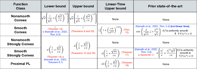
Figure 1: Excess risk for $k=2$, $\widetilde{r}=\sqrt{d}$; we omit logarithms. $\kappa=\beta/\mu$ is the condition number of $F$; $\kappa_{f}=\beta_{f}/\mu$ is the worst-case condition number of $f(\cdot,x)$.

Our Algorithm 3 combines the iterative localization technique of [FKT20, AFKT21] with a noisy clipped subgradient method. With clipped (hence biased) stochastic subgradients and non-Lipschitz/non-smooth $f(\cdot,x)$, the excess risk analysis of our algorithm is harder than in the uniformly Lipschitz setting. Instead of the uniform convergence analysis used in [WXDX20, KLZ22], we derive new results about the stability [KR99, BE02] and generalization error of learning with loss functions that are not uniformly Lipschitz or differentiable; prior results (e.g. [SSSSS09, LY20]) were limited to $\beta_{f}$-smooth and/or $L_{f}$-Lipschitz $f(\cdot,x)$. Specifically, we show the following for non-Lipschitz/non-smooth $f(\cdot,x)$: a) On-average model stability [LY20] implies generalization (Proposition 10); and b) regularized empirical risk minimization is on-average model stable, hence it generalizes (Proposition 11). We combine these results with an empirical error bound for biased, noisy subgradient method to bound the excess risk of our algorithm (Theorem 6). We obtain our strongly convex bound (Theorem 12) by a reduction to the convex case, ala [HK14, FKT20].

We also refine (to describe the dependence on $\widetilde{r}_{k},D,\mu$), extend (to $k\gg 1$), and tighten (for $\mu=0$) the lower bounds of [KLZ22]: see Theorems 13 and 14.

Linear-Time Algorithms for Smooth (Strongly) Convex Losses (Section 4): For convex, $\beta$-smooth $F$, we provide a novel accelerated DP algorithm (Algorithm 4), building on the work of [GL12]. Our algorithm is linear time and attains excess risk that improves over the previous state-of-the-art (not linear time) algorithm [KLZ22, Theorem 5.4] in practical parameter regimes (e.g. $d\gtrsim n^{1/6}$). The excess risk of our algorithm is tight in certain cases: e.g., $d\gtrsim(\epsilon n)^{2/3}$ or “sufficiently smooth” $F$ (see Remark 16). Our excess risk bound holds even if $L_{f}=\infty$, which is the case, for instance, for linear regression with unbounded (e.g. Gaussian) data. To prove our bound, we give the first analysis of accelerated SGD with biased stochastic gradients.

For $\mu$-strongly convex, $\beta$-smooth losses, acceleration results in excessive bias accumulation, so we propose a simple noisy clipped SGD. Our algorithm builds on [KLZ22], but uses a lower-bias clipping mechanism from [BD14] and a new, tighter analysis. We attain excess risk that is near-optimal up to a $\widetilde{\mathcal{O}}((\beta/\mu)^{(k-1)/k})$ factor: see Theorem 17. Our bound strictly improves over the best previous bound of [KLZ22].

First Algorithm for Non-Convex (Proximal-PL) Losses (Section 5): We consider losses satisfying the Proximal Polyak-Łojasiewicz (PPL) inequality [Pol63, KNS16] (Definition 18), an extension of the classical PL inequality to the proximal setting. This covers important models like (some) neural nets, linear/logistic regression, and LASSO [KNS16, LY21]. We propose a DP proximal clipped SGD to attain near-optimal excess risk that almost matches the strongly convex rate: see Theorem 19.

We also provide (in Appendix I) the first shuffle differentially private (SDP) [BEM⁺17, CSU⁺19] algorithms for SO with large worst-case Lipschitz parameter. Our SDP algorithms achieve the same risk bounds as their zCDP counterparts without requiring a trusted curator.

2 Private Heavy-Tailed Mean Estimation Building Blocks

In each iteration of our SO algorithms, we need a way to privately estimate the mean $\nabla F(w_{t})=\mathbb{E}_{x\sim\mathcal{D}}[\nabla f(w_{t},x)]$. If $f(\cdot,x)$ is uniformly Lipschitz, then one can simply draw a random sample $x^{t}$ from $X$ and add noise to the stochastic gradient $\nabla f(w_{t},x^{t})$ to obtain a DP estimator of $\nabla F(w_{t})$: the $\ell_{2}$-sensitivity of the stochastic gradients is bounded by $\sup_{x,x^{\prime}\in\mathcal{X}}\|\nabla f(w_{t},x)-\nabla f(w_{t},x^{\prime})\|\leq 2L_{f}$, so the Gaussian mechanism guarantees DP (by Proposition 22). However, in the setting that we consider, $L_{f}$ (and hence the sensitivity) may be huge, leading the privacy noise variance to also be huge. Thus, we clip the stochastic gradients (to force the sensitivity to be bounded) before adding noise. Specifically, we invoke Algorithm 1 on a batch of $s$ stochastic gradients at each iteration of our algorithms. In Algorithm 1, $\Pi_{C}(z):=\operatorname*{argmin}_{y\in B_{2}(0,C)}\|y-z\|^{2}$ denotes the projection onto the centered $\ell_{2}$ ball of radius $C$ in $\mathbb{R}^{d}$. Lemma 5 bounds the bias and variance of Algorithm 1.

Algorithm 1 $\texttt{MeanOracle1}(\{z_{i}\}_{i=1}^{s};s;C;\frac{\epsilon^{2}}{2})$ [BD14]

1:  Input: $Z=\{z_{i}\}_{i=1}^{s}$, $C>0$, $\epsilon>0$. Set $\sigma^{2}=\frac{4C^{2}}{s^{2}\epsilon^{2}}$ for $\frac{\epsilon^{2}}{2}$-zCDP.

2:  Draw $N\sim\mathcal{N}(0,\sigma^{2}\mathbf{I}_{d})$ and compute $\widetilde{\nu}:=\frac{1}{s}\sum_{i=1}^{s}\Pi_{C}(z_{i})+N$.

3:  Output: $\widetilde{\nu}$.

Lemma 5 ([BD14]).

Let $\{z_{i}\}_{i=1}^{s}\sim\mathcal{D}^{s}$ be $\mathbb{R}^{d}$-valued random vectors with $\mathbb{E}z_{i}=\nu$ and $\mathbb{E}\|z_{i}\|^{k}\leq r^{(k)}$ for some $k\geq 2$. Denote the noiseless average of clipped samples by $\widehat{\nu}:=\frac{1}{s}\sum_{i=1}^{s}\Pi_{C}(z_{i})$ and $\widetilde{\nu}:=\widehat{\nu}+N$. Then, $\|\mathbb{E}\widetilde{\nu}-\nu\|=\|\mathbb{E}\widehat{\nu}-\nu\|\leq\mathbb{E}\|\widehat{\nu}-\nu\|\leq\frac{r^{(k)}}{(k-1)C^{k-1}}$, and $\mathbb{E}\|\widetilde{\nu}-\mathbb{E}\widetilde{\nu}\|^{2}=\mathbb{E}\|\widetilde{\nu}-\mathbb{E}\widehat{\nu}\|^{2}\leq d\sigma^{2}+\frac{r^{(2)}}{s}$.

3 Optimal Rates for Non-Smooth (Strongly) Convex Losses

In this section, we establish the optimal rates (up to logarithms) for the class of DP SCO problems satisfying Assumption 1. We present our result for convex losses in Section 3.1, and our result for strongly convex losses in Section 3.2. In Section 3.3, we provide lower bounds, which show that our upper bounds are tight (up to logarithms).

3.1 Localized Noisy Clipped Subgradient Method for Convex Losses

Our algorithm (Algorithm 3) uses iterative localization [FKT20, AFKT21] with clipping (in Algorithm 2) to handle stochastic subgradients with large norm.

Algorithm 2 Noisy Clipped Regularized Subgradient Method for DP ERM

1:  Input: Data $X\in\mathcal{X}^{n}$, $T\in\mathbb{N}$, stepsize $\eta$, clip thresh. $C$, regularization $\lambda\geq 0$, constraint set $\mathcal{W}$ and initialization $w_{0}\in\mathcal{W}$.

2:  for $t\in\{0,1,\cdots,T-1\}$ do

3:     $\widetilde{\nabla}F_{t}(w_{t}):=\texttt{MeanOracle1}(\{\nabla f(w_{t},x_{i})\}_{i=1}^{n};n;C;\frac{\epsilon^{2}}{2T})$ for subgradients $\nabla f(w_{t},x_{i})$.

4:     $w_{t+1}=\Pi_{\mathcal{W}}\left[w_{t}-\eta\left(\widetilde{\nabla}F_{t}(w_{t})+\lambda(w_{t}-w_{0})\right)\right]$

5:  end for

6:  Output: $w_{T}$.

Algorithm 3 Localized Noisy Clipped Subgradient Method for DP SCO

1:  Input: Data $X\in\mathcal{X}^{n}$, stepsize $\eta$, clip thresh. $\{C_{i}\}_{i=1}^{\log_{2}(n)}$, iteration num. $\{T_{i}\}_{i=1}^{\log_{2}(n)}$.

2:  Initialize $w_{0}\in\mathcal{W}$. Let $l:=\log_{2}(n)$ and $p=1+1/k$.

3:  for $i\in[l]$ do

4:     Set $n_{i}=2^{-i}n,\eta_{i}=4^{-i}\eta$, $\lambda_{i}=\frac{1}{\eta_{i}n_{i}^{p}}$, $T_{i}=\widetilde{\Theta}\left(\frac{1}{\lambda_{i}\eta_{i}}\right)$, and $D_{i}=\frac{4\widetilde{r}_{k}(\sqrt{n}2^{i})^{1/k}}{\lambda_{i}}$.

5:     Draw new batch $\mathcal{B}_{i}$ of $n_{i}=|\mathcal{B}_{i}|$ samples from $X$ without replacement.

6:     Let $\widehat{F}_{i}(w):=\frac{1}{n_{i}}\sum_{j\in\mathcal{B}_{i}}f(w,x_{j})+\frac{\lambda_{i}}{2}\|w-w_{i-1}\|^{2}$.

7:     Use Algorithm 2 with initialization $w_{i-1}$ to minimize $\widehat{F}_{i}$ over $\mathcal{W}_{i}:=\{w\in\mathcal{W}:\|w-w_{i-1}\|\leq D_{i}\}$, for $T_{i}$ iterations with clip threshold $C_{i}$ and noise $\sigma_{i}^{2}=\frac{4C_{i}^{2}T_{i}}{n_{i}^{2}\epsilon^{2}}$. Let $w_{i}$ be the output of Algorithm 2.

8:  end for

9:  Output: $w_{l}$.

The main ideas of Algorithm 3 are:

1. Clipping only the non-regularized component of the subgradient to control sensitivity and bias: Notice that when we call Algorithm 2 in phase $i$ of Algorithm 3, we only clip the subgradients of $f(w,x_{j})$ and not the regularized loss $f(w,x_{j})+\frac{\lambda}{2}\|w-w_{i-1}\|^{2}$. Compared to clipping the full gradient of the regularized loss, our selective clipping approach significantly reduces the bias of our subgradient estimator. This is essential for obtaining our near-optimal excess risk. Further, this reduction in bias comes at no cost to the variance of our subgradient estimator: the $\ell_{2}$-sensitivity of our estimator is unaffected by the regularization term.

2. Solve regularized ERM subproblem with a stable DP algorithm: We run a multi-pass zCDP solver on a regularized empirical loss: Multiple passes let us reduce the noise variance in phase $i$ by a factor of $T_{i}$ (via strong composition for zCDP) and get a more accurate solution to the ERM subproblem. Regularization makes the empirical loss strongly convex, which improves on-average model stability and hence generalization of the obtained solution (see Proposition 10 and 29).

3. Localization [FKT20, ADF⁺21] (i.e. iteratively “zooming in” on a solution): In early phases (small $i$), when we are far away from the optimum $w^{*}$, we use more samples (larger $n_{i}$) and large learning rate $\eta_{i}$ to make progress quickly. As $i$ increases, $w_{i}$ is closer to $w^{*}$, so fewer samples and slower learning rate suffice. Since step size $\eta_{i}$ shrinks (geometrically) faster than $n_{i}$, the effective variance of the privacy noise $\eta_{i}^{2}\sigma_{i}^{2}$ decreases as $i$ increases. This prevents $w_{i+1}$ from moving too far away from $w_{i}$ (and hence from $w^{*}$). We further enforce this localization behavior by increasing the regularization parameter $\lambda_{i}$ and shrinking $D_{i}$ over time. We choose $D_{i}$ as small as possible subject to the constraint that $\operatorname*{argmin}_{w\in\mathcal{W}}\widehat{F}_{i}(w)\in\mathcal{W}_{i}$ with high probability. This constraint ensures that Algorithm 2 can find $w_{i}$ with small expected excess risk.

Next, we provide privacy and excess risk guarantees for Algorithm 3:

Theorem 6.

Grant Assumption 1. Let $\epsilon\leq\sqrt{d}$ and let $f(\cdot,x)$ be convex. Then, there are algorithmic parameters such that Algorithm 3 is $\frac{\epsilon^{2}}{2}$-zCDP, and has excess risk

$$\mathbb{E}F(w_{l})-F^{*}\lesssim\widetilde{r}_{2k}D\left(\frac{1}{\sqrt{n}}+\left(\frac{\sqrt{d\ln(n)}}{\epsilon n}\right)^{\frac{k-1}{k}}\right).$$

Moreover, this excess risk is attained in $\widetilde{\mathcal{O}}(n^{2+1/k})$ subgradient evaluations.

Remark 7 (Improved Computational Complexity for Approximate or Shuffle DP).

If one desires $(\epsilon,\delta)$-DP or $(\epsilon,\delta)$-SDP instead of zCDP, then the subgradient complexity of Algorithm 3 can be improved to $\widetilde{\mathcal{O}}\left(n^{\frac{3}{2}+1/k}\right)$: see Section E.2.

The excess risk bound in Theorem 6 is optimal up to a factor of $\widetilde{\mathcal{O}}(\widetilde{r}_{2k}/\widetilde{r}_{k})$. A key feature of this bound is that it does not depend on $L_{f}$ and holds even for heavy-tailed problems with $L_{f}=\infty$. By contrast, prior works [WXDX20, KLZ22] required uniform $\beta_{f}$-smoothness of $f(\cdot,x)$, which implies the restriction $L_{f}\leq\beta_{f}D$ for loss functions that have a vanishing gradient at some point.

The proof of Theorem 6 consists of three main steps: i) We bound the empirical error of the noisy clipped subgradient subroutine (Lemma 8). ii) We prove that if an algorithm is on-average model stable (Definition 9), then it generalizes (Proposition 10). iii) We bound the on-average model stability of regularized ERM with non-smooth/non-Lipschitz $f(\cdot,x)$ (Proposition 29), leading to an excess population loss bound for Algorithm 2 run on the regularized empirical objective (c.f. line 7 of Algorithm 3). By using these results with the proof technique of [FKT20], we can obtain Theorem 6.

First, we bound the empirical error of the step in line 7 of Algorithm 3, by extending the analysis of noisy subgradient method to biased subgradient oracles:

Lemma 8.

Fix $X\in\mathcal{X}^{n}$ and let $\widehat{F}_{\lambda}(w)=\frac{1}{n}\sum_{i=1}^{n}f(w,x_{i})+\frac{\lambda}{2}\|w-w_{0}\|^{2}$ for $w_{0}\in\mathcal{W}$, where $\mathcal{W}$ is a closed convex domain with diameter $D$. Assume $f(\cdot,x)$ is convex and $\small\widehat{r}_{n}(X)^{(k)}\geq\sup_{w\in\mathcal{W}}\left\{\frac{1}{n}\sum_{i=1}^{n}\|\nabla f(w,x_{i})\|^{k}\right\}$ for all $\nabla f(w,x_{i})\in\partial_{w}f(w,x_{i})$. Denote $\widehat{r}_{n}(X)=\left[\widehat{r}_{n}(X)^{(k)}\right]^{1/k}$ and $\hat{w}=\operatorname*{argmin}_{w\in\mathcal{W}}\widehat{F}_{\lambda}(w)$. Let $\eta\leq\frac{2}{\lambda}$. Then, the output of Algorithm 2 satisfies

$$\mathbb{E}\|w_{T}-\hat{w}\|^{2}\leq\exp\left(-\frac{\lambda\eta T}{2}\right)\|w_{0}-\hat{w}\|^{2}+\frac{8\eta}{\lambda}\left(\widehat{r}_{n}(X)^{2}+\lambda^{2}D^{2}+d\sigma^{2}\right)+\frac{20}{\lambda^{2}}\left(\frac{\widehat{r}_{n}(X)^{(k)}}{(k-1)C^{k-1}}\right)^{2},$$

where $\sigma^{2}=\frac{4C^{2}T}{n^{2}\epsilon^{2}}$.

Detailed proofs for this subsection are deferred to Section E.2.

Our next goal is to bound the generalization error of regularized ERM with convex loss functions that are not differentiable or uniformly Lipschitz. We will use a stability argument to obtain such a bound. Recall the notion of on-average model stability [LY20]:

Definition 9.

Let $X=(x_{1},\cdots,x_{n})$ and $X^{\prime}=(x^{\prime}_{1},\cdots,x^{\prime}_{n})$ be drawn independently from $\mathcal{D}$. For $i\in[n]$, let $X^{i}:=(x_{1},\cdots,x_{i-1},x^{\prime}_{i},x_{i+1},\cdots,x_{n})$. We say randomized algorithm $\mathcal{A}$ has on-average model stability $\alpha$ (i.e. $\mathcal{A}$ is $\alpha$-on-average model stable) if $\mathbb{E}\left[\frac{1}{n}\sum_{i=1}^{n}\|\mathcal{A}(X)-\mathcal{A}(X^{i})\|^{2}\right]\leq\alpha^{2}.$ The expectation is over the randomness of $\mathcal{A}$ and the draws of $X$ and $X^{\prime}$.

On-average model stability is weaker than the notion of uniform stability [BE02], which has been used in DP Lipschitz SCO (e.g. by [BFTT19]); this is necessary for obtaining our learnability guarantees without uniform Lipschitz continuity.

The main result in [LY20] showed that on-average model stable algorithms generalize well if $f(\cdot,x)$ is $\beta_{f}$-smooth for all $x$, which leads to a restriction on $L_{f}$. We show that neither smoothness nor Lipschitz continuity of $f$ is needed to ensure generalizability:

Proposition 10.

Let $f(\cdot,x)$ be convex for all $x$. Suppose $\mathcal{A}:\mathcal{X}^{n}\to\mathcal{W}$ is $\alpha$-on-average model stable. Let $\widehat{F}_{X}(w):=\frac{1}{n}\sum_{i=1}^{n}f(w,x_{i})$ be an empirical loss. Then for any $\zeta>0$,

$$\mathbb{E}[F(\mathcal{A}(X))-\widehat{F}_{X}(\mathcal{A}(X))]\leq\frac{\widetilde{r}^{(2)}}{2\zeta}+\frac{\zeta}{2}\alpha^{2}.$$

Using Proposition 10, we can bound the generalization error and excess (population) risk of regularized ERM:

Proposition 11.

Let $f(\cdot,x)$ be convex, $w_{i-1},y\in\mathcal{W}$, and $\hat{w}_{i}:=\operatorname*{argmin}_{w\in\mathcal{W}}\widehat{F}_{i}(w)$, where $\widehat{F}_{i}(w):=\frac{1}{n_{i}}\sum_{j\in\mathcal{B}_{i}}f(w,x_{j})+\frac{\lambda_{i}}{2}\|w-w_{i-1}\|^{2}$ (c.f. line 6 of Algorithm 3). Then,

$$\mathbb{E}[F(\hat{w}_{i})]-F(y)\leq\frac{2\widetilde{r}^{(2)}}{\lambda_{i}n_{i}}+\frac{\lambda_{i}}{2}\|y-w_{i-1}\|^{2},$$

where the expectation is over both the random draws of $X$ from $\mathcal{D}$ and $\mathcal{B}_{i}$ from $X$.

With the pieces developed above, we can now sketch the proof of Theorem 6:

Sketch of the Proof of Theorem 6.

Privacy: Since the batches $\{\mathcal{B}_{i}\}_{i=1}^{l}$ are disjoint, it suffices to show that $w_{i}$ (produced by $T_{i}$ iterations of Algorithm 2 in line 7 of Algorithm 3) is $\frac{\epsilon^{2}}{2}$-zCDP  $\forall i\in[l]$. The $\ell_{2}$ sensitivity of the clipped subgradient update is $\Delta=\sup_{w,X\sim X^{\prime}}\|\frac{1}{n_{i}}\sum_{j=1}^{n_{i}}\Pi_{C_{i}}(\nabla f(w,x_{j}))-\Pi_{C_{i}}(\nabla f(w,x^{\prime}_{j}))\|\leq 2C_{i}/n_{i}$. (Note that the regularization term does not contribute to sensitivity.) Thus, the privacy guarantees of the Gaussian mechanism (Proposition 22) and the composition theorem for zCDP (Lemma 23) imply that Algorithm 3 is $\frac{\epsilon^{2}}{2}$-zCDP.

Excess risk: First, our choice of $D_{i}$ ensures that $\hat{w}_{i}\in\mathcal{W}_{i}$ for all $i\in[l]$ with high probability $\geq 1-1/\sqrt{n}$, by Chebyshev’s inequality. We will assume that this event occurs in the rest of the proof sketch: see the detailed proof in the Appendix for when this event breaks. Denote $p=1+1/k$. Combining Lemma 8 with Lemma 5 and proper choices of $\eta$ and $T_{i}$, we get:

$$\mathbb{E}\|w_{i}-\hat{w}_{i}\|^{2}\lesssim\eta_{i}^{2}n_{i}^{p}(\widetilde{r}_{k}^{2}n^{1/k}2^{2i/k}+d\sigma_{i}^{2})+\frac{\eta_{i}^{2}n_{i}^{2p}\widetilde{r}^{(2k)}}{C_{i}^{2k-2}}\lesssim\left(\frac{\eta^{2}n^{p}}{32^{i}}\left((\widetilde{r}_{k}^{2}n^{1/k}2^{2i/k}+\frac{dC_{i}^{2}T_{i}}{\epsilon^{2}n_{i}^{2}}+\frac{n^{p}\widetilde{r}^{(2k)}}{C_{i}^{2k-2}2^{pi}}\right)\right).$$ (2)

Now, following the strategy used in the proof of [FKT20, Theorem 4.4], we write $\mathbb{E}F(w_{l})-F(w^{*})=\mathbb{E}[F(w_{l})-F(\hat{w}_{l})]+\sum_{i=1}^{l}\mathbb{E}[F(\hat{w}_{i})-F(\hat{w}_{i-1})]$, where $\hat{w}_{0}:=w^{*}$. Using Eq. 2 and $\widetilde{r}_{k}$-Lipschitz continuity of $F$ (which is implied by Assumption 1), we can bound $\mathbb{E}[F(w_{l})-F(\hat{w}_{l})]$ for the right $\eta$ and $C_{l}$. To bound the sum (second term), we use Proposition 11 to obtain

$$\sum_{i=1}^{l}\mathbb{E}[F(\hat{w}_{i})-F(\hat{w}_{i-1})] \lesssim r^{2}\eta n^{p-1}+\frac{D^{2}}{\eta n^{p}}+\eta\widetilde{r}_{k}^{2}n^{1/k}+\eta\sum_{i=2}^{l}4^{-i}n_{i}^{p}\widetilde{r}_{2k}^{2}\left(\frac{d\ln(n)}{\epsilon^{2}n_{i}^{2}}\right)^{\frac{k-1}{k}}$$

$$\lesssim\eta\left[r^{2}n^{p-1}+\widetilde{r}_{k}^{2}n^{1/k}+\widetilde{r}_{2k}^{2}n^{p}\left(\frac{d\ln(n)}{\epsilon^{2}n^{2}}\right)^{\frac{k-1}{k}}\right]+\frac{D^{2}}{\eta n^{p}},$$

for the right choice of $C_{i}$. Then properly choosing $\eta$ completes the excess risk proof.

Computational complexity: The choice $T_{i}=\widetilde{\mathcal{O}}(n_{i}^{p})=\widetilde{\mathcal{O}}(n_{i}^{1+1/k})$ implies that the number of subgradient evaluations is bounded by $\sum_{i=1}^{l}n_{i}T_{i}=\widetilde{\mathcal{O}}(n^{p+1})=\widetilde{\mathcal{O}}(n^{2+1/k})$. ∎

3.2 The Strongly Convex Case

Following [FKT20], we use a folklore reduction to the convex case (detailed in Section E.3) in order to obtain the following upper bound via Theorem 6:

Theorem 12.

Grant Assumption 1. Let $\epsilon\leq\sqrt{d}$ and let $f(\cdot,x)$ be $\mu$-strongly convex. Then, there is a polynomial-time $\frac{\epsilon^{2}}{2}$-zCDP algorithm $\mathcal{A}$ based on Algorithm 3 with excess risk

$$\mathbb{E}F(\mathcal{A}(X))-F^{*}\lesssim\frac{\widetilde{r}_{2k}^{2}}{\mu}\left(\frac{1}{n}+\left(\frac{\sqrt{d\ln(n)}}{\epsilon n}\right)^{\frac{2k-2}{k}}\right).$$

3.3 Lower Bounds

The work of [KLZ22] proved lower bounds that are tight (by our upper bounds in Section 3) in most parameter regimes for $D=\mu=1$, $\widetilde{r}_{k}=\sqrt{d}$, and $k=\mathcal{O}(1)$. Our (relatively modest) contribution in this subsection is: refining these lower bounds to display the correct dependence on $\widetilde{r}_{k},D,\mu$; tightening the convex lower bound [KLZ22, Theorem 6.4] in the regime $d>n$; and extending [KLZ22, Theorems 6.1 and 6.4] to $k\gg 1$. Our first lower bound holds even for affine functions:

Theorem 13 (Smooth Convex, Informal).

Let $\rho\leq d$. For any $\rho$-zCDP algorithm $\mathcal{A}$, there exist closed convex sets $\mathcal{W},\mathcal{X}\subset\mathbb{R}^{d}$ such that $\|w-w^{\prime}\|\leq 2D$ for all $w,w^{\prime}\in\mathcal{W}$, a $\beta_{f}$-smooth, $L_{f}$-Lipschitz, linear, convex (in $w$) loss $f:\mathcal{W}\times\mathcal{X}\to\mathbb{R}$, and distributions $\mathcal{D}$ and $\mathcal{D^{\prime}}$ on $\mathcal{X}$ such that Assumption 1 holds and if $X\sim\mathcal{D}^{n}$, then

$$\mathbb{E}F(\mathcal{A}(X))-F^{*}=\Omega\left(\widetilde{r}_{k}D\left(\frac{1}{\sqrt{n}}+\min\left\{1,\left(\frac{\sqrt{d}}{\sqrt{\rho}n}\right)^{\frac{k-1}{k}}\right\}\right)\right).$$

Remark 37 (in Appendix F) discusses parameter regimes in which Theorem 13 is strictly tighter than [KLZ22, Theorem 6.4], as well as differences in our proof vs. theirs.

Next, we provide lower bounds for smooth, strongly convex loss functions:

Theorem 14 (Smooth Strongly Convex, Informal).

Let $\rho\leq d$. For any $\rho$-zCDP algorithm $\mathcal{A}$, there exist compact convex sets $\mathcal{W},\mathcal{X}\subset\mathbb{R}^{d}$, a $L_{f}$-Lipschitz, $\mu$-smooth, $\mu$-strongly convex (in $w$) loss $f:\mathcal{W}\times\mathcal{X}\to\mathbb{R}$, and distributions $\mathcal{D}$ and $\mathcal{D^{\prime}}$ on $\mathcal{X}$ such that: Assumption 1 holds, and if $X\sim\mathcal{D}^{n}$, then

$$\mathbb{E}F(\mathcal{A}(X))-F^{*}=\Omega\left(\frac{\widetilde{r}_{k}^{2}}{\mu}\left(\frac{1}{n}+\min\left\{1,\left(\frac{\sqrt{d}}{\sqrt{\rho}n}\right)^{\frac{2k-2}{k}}\right\}\right)\right).$$

Thus, our upper bounds are indeed tight (up to logarithms). Having resolved Question I, next we will develop more computationally efficient, linear-time algorithms for smooth $F(\cdot)$.

4 Linear-Time Algorithms for Smooth (Strongly) Convex Losses

4.1 Noisy Clipped Accelerated SGD for Smooth Convex Losses

Algorithm 4 is a one-pass accelerated algorithm, which builds on (non-private) AC-SA of [GL12]; its privacy and excess risk guarantees are given in Theorem 15.

Algorithm 4 Noisy Clipped Accelerated SGD (AC-SA) for Heavy-Tailed DP SCO

1:  Input: Data $X\in\mathcal{X}^{n}$, iteration number $T\leq n$, stepsize parameters $\{\eta_{t}\}_{t\in[T]},\{\alpha_{t}\}_{t\in[T]}$ with $\alpha_{1}=1,\alpha_{t}\in(0,1)$ $\forall t\geq 2$.

2:  Initialize $w_{0}^{ag}=w_{0}\in\mathcal{W}$ and $t=1$.

3:  for $t\in[T]$ do

4:     $w_{t}^{md}:=(1-\alpha_{t})w_{t-1}^{ag}+\alpha_{t}w_{t-1}$.

5:     Draw new batch $\mathcal{B}_{t}$ (without replacement) of $n/T$ samples from $X$.

6:     $\widetilde{\nabla}F_{t}(w_{t}^{md}):=\texttt{MeanOracle1}(\{\nabla f(w_{t}^{md},x)\}_{x\in\mathcal{B}_{t}};\frac{n}{T};\frac{\epsilon^{2}}{2})$

7:     $w_{t}:=\operatorname*{argmin}_{w\in\mathcal{W}}\left\{\alpha_{t}\langle\widetilde{\nabla}F_{t}(w_{t}^{md}),w\rangle+\frac{\eta_{t}}{2}\|w_{t-1}-w\|^{2}\right\}.$

8:     $w_{t}^{ag}:=\alpha_{t}w_{t}+(1-\alpha_{t})w_{t-1}^{ag}.$

9:  end for

10:  Output: $w_{T}^{ag}$.

Theorem 15 (Informal).

Grant Assumption 1. Let $F$ be convex and $\beta$-smooth. Then, there are parameters such that Algorithm 4 is $\frac{\epsilon^{2}}{2}$-zCDP and:

$$\mathbb{E}F(w_{T}^{ag})-F^{*}\lesssim\widetilde{r}_{k}D\left[\frac{1}{\sqrt{n}}+\max\left\{\left(\left(\frac{\beta D}{\widetilde{r}_{k}}\right)^{1/4}\frac{\sqrt{d}}{\epsilon n}\right)^{\frac{4(k-1)}{5k-1}},\left(\frac{\sqrt{d}}{\epsilon n}\right)^{\frac{k-1}{k}}\right\}\right].$$ (3)

Moreover, Algorithm 4 uses at most $n$ gradient evaluations.

The key ingredient used to prove Eq. 3 is a novel convergence guarantee for AC-SA with biased, noisy stochastic gradients: see Proposition 40 in Section G.1. Combining Proposition 40 with Lemma 5 and a careful choice of stepsizes, clip threshold, and $T$ yields Theorem 15.

Remark 16 (Optimal rate for “sufficiently smooth” functions).

Note that the upper bound Eq. 3 scales with the smoothness parameter $\beta$. Thus, for sufficiently small $\beta$, the optimal rates are attained. For example, if $k=2$, the upper bound in Eq. 3 matches the lower bound in Theorem 13 when $\small\beta\lesssim\frac{\widetilde{r}_{k}}{D}\left(\frac{d^{5}}{\epsilon n}\right)^{1/18}\normalsize$; e.g. if $\beta$ and $D$ are constants and $d\geq(\epsilon n)^{1/5}$. In particular, for affine functions (which were not addressed in [WXDX20, KLZ22] since these works assume $\nabla F(w^{*})=0$), $\beta=0$ and Algorithm 4 is optimal.

Having discussed the dependence on $\beta$, let us focus on understanding how the bound in Theorem 15 scales with $n,d$ and $\epsilon$. Thus, let us fix $\small\beta=D=1\normalsize$ and $\small\widetilde{r}_{k}=\sqrt{d}\normalsize$ for simplicity. If $k=2$, then the bound in Eq. 3 simplifies to $\small\mathcal{O}\left(\sqrt{\frac{d}{n}}+\max\left\{\frac{d^{2/3}}{(\epsilon n)^{4/9}},\frac{d^{3/4}}{\sqrt{\epsilon n}}\right\}\right),$ whereas the lower bound in Theorem 13 (part 2) is $\small\Omega\left(\sqrt{\frac{d}{n}}+\frac{d^{3/4}}{\sqrt{\epsilon n}}\right)\normalsize$. Therefore, the bound in Eq. 3 is tight if $d^{3/2}\gtrsim\epsilon n$. For general $n,d,\epsilon$, Eq. 3 is nearly tight up to a multiplicative factor of $\small\left(\frac{\epsilon n}{d^{3/2}}\right)^{1/18}\normalsize$. By comparison, the previous state-of-the-art (not linear-time) bound for $\epsilon\approx 1$ was $\small\mathcal{O}\left(\frac{d}{\sqrt{n}}\right)\normalsize$ [KLZ22, Theorem 5.4]. Our bound Eq. 3 improves over [KLZ22, Theorem 5.4] if $\small d\gtrsim n^{1/6}\normalsize$, which is typical in practical ML applications. As $k\to\infty$,  Eq. 3 becomes $\small\mathcal{O}\left(\sqrt{\frac{d}{n}}+\left(\frac{d}{n}\right)^{4/5}\right)\normalsize$ for $\epsilon\approx 1$, which is strictly better than the bound in [KLZ22, Theorem 5.4].

4.2 Noisy Clipped SGD for Strongly Convex Losses

Our algorithm for strongly convex losses (Algorithm 6 in Section G.2) is a simple one-pass noisy clipped SGD. Compared to the algorithm of [KLZ22], our approach differs in the choice of MeanOracle, step size, and iterate averaging weights, and in our analysis.

Theorem 17 (Informal).

Grant Assumption 1. Let $F$ be $\mu$-strongly convex, $\beta$-smooth with $\frac{\beta}{\mu}\leq n/\ln(n)$. Then, there are algorithmic parameters such that Algorithm 6 is $\frac{\epsilon^{2}}{2}$-zCDP and:

$$\mathbb{E}F(\widehat{w}_{T})-F^{*}\lesssim\frac{\widetilde{r}_{k}^{2}}{\mu}\left(\frac{1}{n}+\left(\frac{\sqrt{d(\beta/\mu)\ln(n)}}{\epsilon n}\right)^{\frac{2k-2}{k}}\right).$$ (4)

Moreover, Algorithm 6 uses at most $n$ gradient evaluations.

The bound Eq. 4 is optimal up to a $\widetilde{\mathcal{O}}((\beta/\mu)^{(k-1)/k})$ factor and improves over the best previous bound in [KLZ22, Theorem 5.6] by removing the dependence on $\beta_{f}$ (which can be much larger than $\beta$ in the presence of outliers). The proof of Theorem 17 (in Section G.2) relies on a novel convergence guarantee for projected SGD with biased noisy stochastic gradients: Proposition 42. Compared to results in [ADF⁺21] for convex ERM and [AS20] for PL SO, Proposition 42 is tighter, which is needed to obtain near-optimal excess risk: we leverage smoothness and strong convexity. Our new analysis also avoids the issue in the proofs of (the ICML versions of) [WXDX20, KLZ22].

5 Algorithm for Non-Convex Proximal-PL Loss Functions

Assume: $f(w,x)=f^{0}(w,x)+f^{1}(w)$; $f^{0}(\cdot,x)$ is differentiable (maybe non-convex); $f^{1}$ is proper, closed, and convex (maybe non-differentiable) for all $x\in\mathcal{X}$; and $F(w)=F^{0}(w)+f^{1}(w)=\mathbb{E}_{x\sim\mathcal{D}}[f^{0}(w,x)]+f^{1}(w)$ satisfies the Proximal-PL condition [KNS16]:

Definition 18 ($\mu$-PPL).

Let $F(w)=F^{0}(w)+f^{1}(w)$ be bounded below; $F^{0}$ is $\beta$-smooth and $f^{1}$ is convex. $F$ satisfies Proximal Polyak-Łojasiewicz inequality with parameter $\mu>0$ if

$$\mu[F(w)-\inf_{w^{\prime}}F(w^{\prime})] \leq-\beta\min_{y}\left[\langle\nabla F^{0}(w),y-w\rangle+\frac{\beta}{2}\|y-w\|^{2}+f^{1}(y)-f^{1}(w)\right],~{}\forall~{}w\in\mathbb{R}^{d}.$$

Definition 18 generalizes the classical PL condition ($f^{1}=0$), allowing for constrained optimization or non-smooth regularizer depending on $f^{1}$ [Pol63, KNS16].

Recall that the proximal operator of a convex function $g$ is defined as $\texttt{{prox}}_{\eta g}(z):=\operatorname*{argmin}_{y\in\mathbb{R}^{d}}\left(\eta g(y)+\frac{1}{2}\|y-z\|^{2}\right)$ for $\eta>0$. We propose Noisy Clipped Proximal SGD (Algorithm 8 in Appendix H) for PPL losses. The algorithm runs as follows. For $t\in[T]$: first draw a new batch $\mathcal{B}_{t}$ (without replacement) of $n/T$ samples from $X$; let $\widetilde{\nabla}F_{t}^{0}(w_{t}):=\texttt{MeanOracle1}(\{\nabla f^{0}(w_{t},x)\}_{x\in\mathcal{B}_{t}};\frac{n}{T};\frac{\epsilon^{2}}{2})$; then update $w_{t+1}=\texttt{{prox}}_{\eta_{t}f^{1}}\left(w_{t}-\eta_{t}\widetilde{\nabla}F_{t}^{0}(w_{t})\right)$. Finally, return the last iterate, $w_{T}$. Thus, the algorithm is linear time. Furthermore:

Theorem 19 (Informal).

Grant Assumption 1. Let $F$ be $\mu$-PPL for $\beta$-smooth $F^{0}$, with $\frac{\beta}{\mu}\leq n/\ln(n)$. Then, there are parameters such that Algorithm 8 is $\frac{\epsilon^{2}}{2}$-zCDP, and:

$$\mathbb{E}F(w_{T})-F^{*}\lesssim\frac{\widetilde{r}_{k}^{2}}{\mu}\left(\left(\frac{\sqrt{d}}{\epsilon n}(\beta/\mu)\ln(n)\right)^{\frac{2k-2}{k}}+\frac{(\beta/\mu)\ln(n)}{n}\right).$$

Moreover, Algorithm 8 uses at most $n$ gradient evaluations.

The bound in Theorem 19 nearly matches the smooth strongly convex (hence PPL) lower bound in Theorem 14 up to $\widetilde{\mathcal{O}}((\beta/\mu)^{(2k-2)/2})$, and is attained without convexity.

To prove Theorem 19, we derive a convergence guarantee for proximal SGD with generic biased, noisy stochastic gradients in terms of the bias and variance of the oracle (see Proposition 45). We then apply this guarantee for MeanOracle1 (Algorithm 1) with carefully chosen stepsizes, clip threshold, and $T$, using Lemma 5. Proposition 45 generalizes [AS20, Theorem 6]–which covered the unconstrained classical PL problem–to the proximal setting. However, the proof of Proposition 45 is very different from the proof of [AS20, Theorem 6], since prox makes it hard to bound excess risk without convexity when the stochastic gradients are biased/noisy. Instead, our proof builds on the proof of [LGR22, Theorem 3.1], using techniques from the analysis of objective perturbation [CMS11, KST12]. See Appendix H for details.

6 Concluding Remarks and Open Questions

This paper was motivated by practical problems in which data contains outliers and potentially heavy tails, causing the worst-case Lipschitz parameter of the loss over all data points to be prohibitively large. In such cases, existing bounds for DP SO that scale with the worst-case Lipschitz parameter become vacuous. Thus, we operated under the more relaxed assumption of stochastic gradient distributions having bounded $k$-th moments. The $k$-th moment bound can be much smaller than the worst-case Lipschitz parameter in practice. For (strongly) convex loss functions, we established the asymptotically optimal rates (up to logarithms), even with non-differentiable losses. We also provided linear-time algorithms for smooth losses that are optimal in certain practical parameter regimes, but suboptimal in general. An interesting open question is: does there exist a linear-time algorithm with optimal excess risk? We also initiated the study of non-convex DP SO without uniform Lipschitz continuity, showing that the optimal strongly convex rates can nearly be attained without convexity, via the proximal-PL condition. We leave the treatment of general non-convex losses for future work.

Appendix

Appendix A Additional Discussion of Related Work

DP SCO Without Uniform Lipschitz Continuity: The study of DP SCO without uniformly Lipschitz continuous loss functions was initiated by [WXDX20], who provided upper bounds for smooth convex/strongly convex loss. The work of [KLZ22] provided lower bounds and improved, yet suboptimal, upper bounds for the convex case. Both of the works [WXDX20, KLZ22] require $f$ to be $\beta_{f}$-smooth. It is also worth mentioning that [WXDX20, KLZ22] restricted attention to losses satisfying $\nabla F(w^{*})=0$ for $w^{*}\in\mathcal{W}$, i.e. $\mathcal{W}$ is a compact set containing the unconstrained optimum $w^{*}=\operatorname*{argmin}_{w\in\mathbb{R}^{d}}F(w)\in\mathcal{W}$. By comparison, we consider the more general constrained optimization problem $\min_{w\in\mathcal{W}}F(w)$, where $\mathcal{W}$ need not contain the global unconstrained optimum.

Here we provide a brief discussion of the techniques used in [WXDX20, KLZ22]. The work of [WXDX20] used a full batch (clipped, noisy) gradient descent based algorithm, building on the heavy-tailed mean estimator of [Hol19]. They bounded the excess risk of their algorithm by using a uniform convergence [Vap99] argument, resulting in a suboptimal dependence on the dimension $d$. The work of [KLZ22] used essentially the same approach as [WXDX20], but obtained an improved rate with a more careful analysis. However, as discussed, the bound in [KLZ22] is $\mathcal{O}\left(rD\sqrt{\frac{d}{n}}\right)$ when $\epsilon\approx 1$, which is still suboptimal.

More recently, DP optimization with outliers was studied in special cases of sparse learning [HNXW21], multi-arm bandits [TWZW21], and $\ell_{1}$-norm linear regression [WX22].

DP ERM and DP GLMs without Uniform Lipschitz continuity: The work of [ADF⁺21] provides bounds for constrained DP ERM with arbitrary convex loss functions using a Noisy Clipped SGD algorithm that is similar to our Algorithm 6, except that their algorithm is multi-pass and ours is one-pass. In a concurrent work, [DKX⁺22] considered DP ERM in the unconstrained setting with convex and non-convex loss functions. Their algorithm, noisy clipped SGD, is also similar to Algorithm 6 and the algorithm of [ADF⁺21]. The results in [DKX⁺22] are not directly comparable to [ADF⁺21] since [DKX⁺22] consider the unconstrained setting while [ADF⁺21] consider the constrained setting, but the rates in [ADF⁺21] are faster. [DKX⁺22] also analyzes the convergence of noisy clipped SGD with smooth non-convex loss functions.

The works of [SSTT21, ABG⁺22] consider generalized linear models (GLMs), a particular subclass of convex loss functions and provide empirical and population risk bounds for the unconstrained DP optimization problem. The unconstrained setting is not comparable to the constrained setting that we consider here: in the unconstrained case, a dimension-independent upper bound is achievable, whereas our lower bounds (which apply to GLMs) imply that a dependence on the dimension $d$ is necessary in the constrained case.

Other works on gradient clipping: The gradient clipping technique (and adaptive variants of it) has been studied empirically in works such as [ACG⁺16, CWH20, ATMR21], to name a few. The work of [CWH20] shows that gradient clipping can prevent SGD from converging, and describes the clipping bias with a disparity measure between the gradient distribution and a geometrically symmetric distribution.

Optimization with biased gradient oracles: The works [AS20, ADF⁺21] analyze SGD with biased gradient oracles. Our work provides a tighter bound for smooth, strongly convex functions and analyzes accelerated SGD and proximal SGD with biased gradient oracles.

DP SO with Uniformly Lipschitz loss functions: In the absence of outlier data, there are a multitude of works studying uniformly Lipschitz DP SO, mostly in the convex/strongly convex case. We do not attempt to provide a comprehensive list of these here, but will name the most notable ones, which provide optimal or state-of-the-art utility guarantees. The first suboptimal bounds for DP SCO were provided in [BST14]. The work of [BFTT19] established the optimal rate for non-strongly convex DP SCO, by bounding the uniform stability of Noisy DP SGD (without clipping). The strongly convex case was addressed by [FKT20], who also provided optimal rates in linear times for sufficiently smooth, convex losses. Since then, other works have provided faster and simpler (optimal) algorithms for the non-smooth DP SCO problem [BFGT20, AFKT21, KLL21, BGM21] and considered DP SCO with different geometries [AFKT21, BGN21]. State-of-the-art rates for DP SO with the proximal PL condition are due to [LGR22].

Appendix B Other Bounded Moment Conditions Besides Assumption 1

In this section, we give the alternate bounded moment assumption made in [WXDX20, KLZ22] and a third bounded moment condition, and discuss the relationships between these assumptions. The notation presented here will be necessary in order to state the sharper versions of our linear-time excess risk bounds and the asymptotically optimal excess risk bounds under the coordinate-wise assumption of [WXDX20, KLZ22] (which our Algorithm 3 also attains). First, we introduce a relaxation of Assumption 1:

Assumption 2.

There exists $k\geq 2$ and $r^{(k)}>0$ such that $\sup_{w\in\mathcal{W}}\mathbb{E}\left[\|\nabla f(w,x)\|_{2}^{k}\right]\leq r^{(k)}$, for all subgradients $\nabla f(w,x_{i})\in\partial_{w}f(w,x_{i})$. Denote $r_{k}:=(r^{(k)})^{1/k}$.

Assumption 1 implies Assumption 2 for $r\leq\widetilde{r}$. Next, we precisely state the coordinate-wise moment bound assumption that is used in [WXDX20, KLZ22] for differentiable $f$:

Assumption 3.

(Used by [WXDX20, KLZ22] , but not in this work) There exists $k\geq 2$ and $\gamma>0$ such that $\sup_{w\in\mathcal{W}}\mathbb{E}|\langle\nabla f(w,x)-\nabla F(w),e_{j}\rangle|^{k}\leq\gamma$, for all $j\in[d]$, where $e_{j}$ denotes the $j$-th standard basis vector in $\mathbb{R}^{d}$. Also, $L\triangleq\sup_{w\in\mathcal{W}}\|\nabla F(w)\|\leq\sqrt{d}\gamma^{1/k}$.

Lemma 20 allows us compare our results in Section 4 obtained under Assumption 2 to the results in [WXDX20, KLZ22], which require Assumption 3.

Lemma 20.

Suppose Assumption 3 holds. Then, Assumption 2 holds for $r_{k}\leq 4\sqrt{d}\gamma^{1/k}$.

Proof.

We use the following inequality, which can easily be verified inductively, using Cauchy-Schwartz and Young’s inequalities: for any vectors $u,v\in\mathbb{R}^{d}$, we have

$$\|u\|^{k}\leq 2^{k-1}\left(\|u-v\|^{k}+\|v\|^{k}\right).$$ (5)

Therefore,

$$r^{(k)} =\sup_{w\in\mathcal{W}}\mathbb{E}\|\nabla f(w,x)\|^{k}$$

$$\leq 2^{k-1}\left(\sup_{w\in\mathcal{W}}\mathbb{E}\|\nabla f(w,x)-\nabla F(w)\|^{k}+L^{k}\right)$$

$$=2^{k-1}\left(\sup_{w\in\mathcal{W}}\mathbb{E}\left[\left\{\sum_{j=1}^{d}|\langle\nabla f(w,x)-\nabla F(w),e_{j}\rangle|^{2}\right\}^{k/2}\right]+L^{k}\right)$$

$$\leq(2L)^{k}+2^{k}d^{k/2}\sup_{w\in\mathcal{W}}\mathbb{E}\left[\frac{1}{d}\sum_{j=1}^{d}|\langle\nabla f(w,x)-\nabla F(w),e_{j}\rangle|^{k}\right],$$

where we used convexity of the function $\phi(y)=y^{k/2}$ for all $y\geq 0,k\geq 2$ and Jensen’s inequality in the last inequality. Now using linearity of expectation and Assumption 3 gives us

$$r^{(k)}\leq 2^{k}\left(L^{k}+d^{k/2}\gamma\right)\leq 2^{k+1}d^{k/2}\gamma,$$

since $L^{k}\leq d^{k/2}\gamma$ by hypothesis. ∎

Remark 21.

Since Assumption 2 is implied by Assumption 3, the upper bounds that we obtain under Assumption 2 also hold (up to constants) if we grant Assumption 3 instead, with $r\leftrightarrow\sqrt{d}\gamma^{1/k}$. Also, in Section E.4, we will use Lemma 20 to show that our optimal excess risk bounds under Assumption 1 imply asymptotically optimal excess risk bounds under Assumption 3.

Appendix C Correcting the Errors in the Strongly Convex Upper Bounds Claimed in [KLZ22, WXDX20]

While the ICML 2022 paper [KLZ22, Theorem 5.6] claimed an upper bound for smooth strongly convex losses that is tight up to a factor of $\widetilde{\mathcal{O}}(\kappa_{f}^{2})$—where $\kappa_{f}=\beta_{f}/\mu$ is the uniform condition number of $f(\cdot,x)$ over all $x\in\mathcal{X}$–we identify an issue with their proof that invalidates their result. A similar issue appears in the proof of [WXDX20, Theorems 5 and 7], which [KLZ22] built upon. We then show how to salvage a correct upper bound within the framework of [KLZ22], albeit at the cost of an additional factor of $\kappa_{f}$.

The proof of [KLZ22, Theorem 5.6] relies on [KLZ22, Theorem 3.2]. The proof of [KLZ22, Theorem 3.2], in turn, bounds $\mathbb{E}\|w_{T}-w^{*}\|\leq\frac{(\lambda+L)(M+1)G}{\lambda L}$ in the notation of [KLZ22], where $L$ is the smoothness parameter, $\lambda$ is the strong convexity parameter (so $L\geq\lambda$), and $M$ is the diameter of $\mathcal{W}$. Then, it is incorrectly deduced that $\mathbb{E}[\|w_{T}-w^{*}\|^{2}]\leq\left(\frac{(\lambda+L)(M+1)G}{\lambda L}\right)^{2}$ (final line of the proof). Notice that $\mathbb{E}[\|w_{T}-w^{*}\|^{2}]$ can be much larger than $(\mathbb{E}\|w_{T}-w^{*}\|)^{2}$ in general: for example, if $\|w_{T}-w^{*}\|$ has the Pareto distribution with shape parameter $\alpha\in(1,2]$ and scale parameter $1$, then $(\mathbb{E}\|w_{T}-w^{*}\|)^{2}=\left(\frac{\alpha}{\alpha-1}\right)^{2}\ll\mathbb{E}(\|w_{T}-w^{*}\|^{2})=\infty$.

As a first attempt to correct this issue, one could use Young’s inequality to instead bound

$$\mathbb{E}[\|w_{T}-w^{*}\|^{2}] \leq 2\left(1-\frac{2\lambda L}{(\lambda+L)^{2}}\right)\mathbb{E}[\|w_{T-1}-w^{*}\|^{2}]+\frac{2G^{2}}{(\lambda+L)^{2}}$$

$$\leq\left[2\left(1-\frac{2\lambda L}{(\lambda+L)^{2}}\right)\right]^{T}\|w_{0}-w^{*}\|^{2}+\frac{2G^{2}}{(\lambda+L)^{2}}\sum_{t=0}^{T-1}\left[2\left(1-\frac{2\lambda L}{(\lambda+L)^{2}}\right)\right]^{t},$$

but the geometric series above diverges to $+\infty$ as $T\to\infty$, since $2\left(1-\frac{2\lambda L}{(\lambda+L)^{2}}\right)\geq 1\iff(\lambda-L)^{2}\geq 0$.

Next, we show how to modify the proof of [KLZ22, Theorem 5.6] in order to obtain a correct excess risk upper bound of

$$\widetilde{\mathcal{O}}\left(\frac{\gamma^{2/k}}{\mu}d\left[\frac{(\beta_{f}/\mu)^{3}}{n}+\left(\frac{\sqrt{d(\beta_{f}/\mu)^{3}}}{\epsilon n}\right)^{(2k-2)/k}\right]\right)$$ (6)

(in our notation). This correction was derived in collaboration with the authors of [KLZ22], who have also updated the arXiv version of their paper accordingly. By waiting until the very of the proof of [KLZ22, Theorem 3.2] to take expectation, we can derive

$$\|w_{t}-w^{*}\| \leq\left(1-\frac{\lambda L}{(\lambda+L)^{2}}\right)\|w_{t-1}-w^{*}\|+\frac{\|\widetilde{\nabla}F(w_{t-1})-\nabla F(w_{t-1})\|}{\lambda+L}$$ (7)

for all $t$, where we use their $L=\beta_{f}$ and $\lambda=\mu$ notation but our notation $F$ and $\widetilde{\nabla}F$ for the population loss and its biased noisy gradient estimate (instead of their $L_{\mathcal{D}}$ notation). By iterating Eq. 7, we can get

$$\|w_{T}-w^{*}\| \leq\left(1-\frac{2\lambda L}{(\lambda+L)^{2}}\right)^{T}\|w_{0}-w^{*}\|+\sum_{t=0}^{T-1}\left(1-\frac{2\lambda L}{(\lambda+L)^{2}}\right)^{t}\left[\frac{\|\widetilde{\nabla}F(w_{T-t})-\nabla F(w_{T-t})\|}{\lambda+L}\right].$$

Squaring both sides and using Cauchy-Schwartz, we get

$$\|w_{T}-w^{*}\|^{2} \leq 2\left(1-\frac{2\lambda L}{(\lambda+L)^{2}}\right)^{2T}\|w_{0}-w^{*}\|^{2}+T\sum_{t=0}^{T-1}\left(1-\frac{2\lambda L}{(\lambda+L)^{2}}\right)^{2t}\left[\frac{\|\widetilde{\nabla}F(w_{T-t})-\nabla F(w_{T-t})\|}{\lambda+L}\right]^{2}.$$

Using $L$-smoothness of $F$ and the assumption made in [KLZ22] that $\nabla F(w^{*})=0$, and then taking expectation yields

$$\mathbb{E}F(w_{T})-F^{*}\lesssim L\|w_{0}-w^{*}\|^{2}\left(1-\frac{2\lambda L}{(\lambda+L)^{2}}\right)^{2T}+TG^{2}\frac{L}{\lambda},$$ (8)

where $G^{2}\geq\mathbb{E}\left[\|\widetilde{\nabla}F(w_{T-t})-\nabla F(w_{T-t})\|^{2}\right]$ for all $t$. It is necessary and sufficient to choose $T=\widetilde{\Omega}(L/\lambda)$ to make the first term in the right-hand side of Eq. 8 less than the second term (up to logarithms). With this choice of $T$, we get

$$\mathbb{E}F(w_{T})-F^{*}=\widetilde{\mathcal{O}}\left(G^{2}\kappa_{f}^{2}\right),$$ (9)

where $\kappa_{f}=L/\lambda$. Next, we apply the bound on $G^{2}$ for the MeanOracle that is used in [KLZ22]; this bound is stated in the version of [KLZ22, Lemma B.5] that appears in the updated (November 1, 2022) arXiv version of their paper. The bound (for general $\gamma$) is $G^{2}=\widetilde{\mathcal{O}}\left(\gamma^{2/k}\left[\frac{Td}{n}+d\left(\frac{\sqrt{d}T^{3/2}}{\epsilon n}\right)^{(2k-2)/k}\right]\right)$. Plugging this bound on $G^{2}$ into Eq. 9 yields Eq. 6.

Appendix D More Differential Privacy Preliminaries

We collect some basic facts about DP algorithms that will be useful in the proofs of our results. Our algorithms use the Gaussian mechanism to achieve zCDP:

Proposition 22.

[BS16, Proposition 1.6] Let $q:\mathcal{X}^{n}\to\mathbb{R}$ be a query with $\ell_{2}$-sensitivity $\Delta:=\sup_{X\sim X^{\prime}}\|q(X)-q(X^{\prime})\|$. Then the Gaussian mechanism, defined by $\mathcal{M}:\mathcal{X}^{n}\to\mathbb{R}$, $M(X):=q(X)+u$ for $u\sim\mathcal{N}(0,\sigma^{2})$, is $\rho$-zCDP if $\sigma^{2}\geq\frac{\Delta^{2}}{2\rho}$.

The (adaptive) composition of zCDP algorithms is zCDP, with privacy parameters adding:

Lemma 23.

[BS16, Lemma 2.3] Suppose $\mathcal{A}:\mathcal{X}^{n}\to\mathcal{Y}$ satisfies $\rho$-zCDP and $\mathcal{A}^{\prime}:\mathcal{X}^{n}\times\mathcal{Y}\to\mathcal{Z}$ satisfies $\rho^{\prime}$-zCDP (as a function of its first argument). Define the composition of $\mathcal{A}$ and $\mathcal{A}^{\prime}$, $\mathcal{A}^{\prime\prime}:\mathcal{X}^{n}\to\mathcal{Z}$ by $\mathcal{A}^{\prime\prime}(X)=\mathcal{A}^{\prime}(X,\mathcal{A}(X))$. Then $\mathcal{A}^{\prime\prime}$ satisfies $(\rho+\rho^{\prime})$-zCDP. In particular, the composition of $T$ $\rho$-zCDP mechanisms is a $T\rho$-zCDP mechanism.

The definitions of DP and zCDP given above do not dictate how the algorithm $\mathcal{A}$ operates. In particular, they allow $\mathcal{A}$ to send sensitive data to a third party curator/analyst, who can then add noise to the data. However, in certain practical applications (e.g. federated learning [KMA⁺19]), there is no third party that can be trusted to handle sensitive user data. On the other hand, it is often more realistic to have a secure shuffler (a.k.a. mixnet): in each iteration of the algorithm, the shuffler receives encrypted noisy reports (e.g. noisy stochastic gradients) from each user and applies a uniformly random permutation to the $n$ reports, thereby anonymizing them (and amplifying privacy) [BEM⁺17, CSU⁺19, EFM⁺20, FMT20]. An algorithm is shuffle private if all of these “shuffled” reports are DP:

Definition 24.

(Shuffle Differential Privacy [BEM⁺17, CSU⁺19]) A randomized algorithm is $(\epsilon,\delta)$-shuffle DP (SDP) if the collection of reports output by the shuffler satisfies Definition 1.

Appendix E Details and Proofs for Section 3: Optimal Rates for (Strongly) Convex Losses

In order to precisely state (sharper forms of) Theorems 6 and 12, we will need to introduce some notation.

E.1 Notation

For a batch of data $X\in\mathcal{X}^{m}$, we define the $k$-th empirical moment of $f(w,\cdot)$ by

$$\widehat{r}_{m}(X)^{(k)}=\sup_{w\in\mathcal{W}}\sup_{\{\nabla f(w,x_{i})\in\partial_{w}f(w,x_{i})\}}\frac{1}{m}\sum_{i=1}^{m}\|\nabla f(w,x_{i})\|^{k},$$

where the supremum is also over all subgradients $\nabla f(w,x_{i})\in\partial_{w}f(w,x_{i})$ in case $f$ is not differentiable. For $X\sim\mathcal{D}^{m}$, we denote the $k$-th expected empirical moment by

$$\widetilde{e}_{m}^{(k)}:=\mathbb{E}[\widehat{r}_{m}(X)^{(k)}]$$

and let

$$\widetilde{r}_{k,m}:=(\widetilde{e}_{m}^{(k)})^{1/k}.$$

Note that $\widetilde{r}_{k,1}=\widetilde{r}_{k}$. Our excess risk upper bounds will depend on a weighted average of the expected empirical moments for different batch sizes $m\in\{1,2,4,8,\cdots,n\}$, with more weight being given to $\widetilde{r}_{m}$ for large $m$ (which are smaller, by Lemma 25 below): for $n=2^{l}$, define

$$\widetilde{R}_{k,n}:=\sqrt{\sum_{i=1}^{l}2^{-i}\widetilde{r}_{k,n_{i}}^{2}},$$

where $n_{i}=2^{-i}n$.

Lemma 25.

Under Assumptions 2 and 1, we have: $\widetilde{r}^{(k)}=\widetilde{e}_{1}^{(k)}\geq\widetilde{e}_{2}^{(k)}\geq\widetilde{e}_{4}^{(k)}\geq\widetilde{e}_{8}^{(k)}\geq\cdots\geq r^{(k)}$. In particular, $\widetilde{R}_{k,n}\leq\widetilde{r}_{k}$.

Proof.

Let $l\in\mathbb{N}$, $n=2^{l}$ and consider

$$\widehat{r}_{n}(X)^{(k)} =\frac{1}{n}\sup_{w}\left(\sum_{i=1}^{n/2}\|\nabla f(w,x_{i})\|^{k}+\sum_{i=n/2+1}^{n}\|\nabla f(w,x_{i})\|^{k}\right)$$

$$\leq\frac{1}{n}\left(\sup_{w}\sum_{i=1}^{n/2}\|\nabla f(w,x_{i})\|^{k}+\sup_{w}\sum_{i=n/2+1}^{n}\|\nabla f(w,x_{i})\|^{k}\right).$$

Taking expectations over the random draw of $X\sim\mathcal{D}^{n}$ yields $\widetilde{e}_{n}^{(k)}\leq\widetilde{e}_{n/2}^{(k)}$. Thus, $\widetilde{R}_{k,n}\leq\widetilde{r}_{k}$ by the definition of $\widetilde{R}_{n}$. ∎

E.2 Localized Noisy Clipped Subgradient Method (Section 3.1)

We begin by proving the technical ingredients that will be used in the proof of Theorem 6. First, we will prove a variant of Lemma 5 that bounds the bias and variance of the subgradient estimator in Algorithm 2.

Lemma 26.

Let $\widehat{F}_{\lambda}(w)=\frac{1}{n}\sum_{i=1}^{n}f(w,x_{i})+\frac{\lambda}{2}\|w-w_{0}\|^{2}$ be a regularized empirical loss on a closed convex domain $\mathcal{W}$ with $\ell_{2}$-diameter $D$. Let $\widetilde{\nabla}F_{\lambda}(w_{t})=\nabla\widehat{F}_{\lambda}(w_{t})+b_{t}+N_{t}=\frac{1}{n}\sum_{i=1}^{n}\Pi_{C}(\nabla f(w,x_{i}))+\lambda(w-w_{0})+N_{t}$ be the biased, noisy subgradients of the regularized empirical loss in Algorithm 2, with $N_{t}\sim\mathcal{N}(0,\sigma^{2}\mathbf{I}_{d})$ and $b_{t}=\frac{1}{n}\sum_{i=1}^{n}\Pi_{C}(\nabla f(w_{t},x_{i}))-\frac{1}{n}\sum_{i=1}^{n}\nabla f(w_{t},x_{i})$. Assume $\small\widehat{r}_{n}(X)^{(k)}\geq\sup_{w\in\mathcal{W}}\left\{\frac{1}{n}\sum_{i=1}^{n}\|\nabla f(w,x_{i})\|^{k}\right\}$ for all $\nabla f(w,x_{i})\in\partial_{w}f(w,x_{i})$. Then, for any $T\geq 1$, we have:

$$\hat{B}:=\sup_{t\in[T]}\|b_{t}\|\leq\frac{\widehat{r}_{n}(X)^{(k)}}{(k-1)C^{k-1}}$$

and

$$\hat{\Sigma}^{2}:=\sup_{t\in[T]}\mathbb{E}\|N_{t}\|^{2}=d\sigma^{2}.$$

Proof.

Fix any $t$. We have

$$\|b_{t}\| =\left\|\frac{1}{n}\sum_{i=1}^{n}\Pi_{C}(\nabla f(w_{t},x_{i}))-\frac{1}{n}\sum_{i=1}^{n}\nabla f(w_{t},x_{i})\right\|$$

$$\leq\frac{1}{(k-1)C^{k-1}}\left[\frac{1}{n}\sum_{i=1}^{n}\|\nabla f(w_{t},x_{i})\|^{k}\right],$$ (10)

by Lemma 5 applied with $\mathcal{D}$ as the empirical distribution on $X$, and $z_{i}$ in Lemma 5 corresponding to $\nabla f(w_{t},x_{i})$ in Section E.2. Taking supremum over $t$ of both sides of Section E.2 and recalling the definition of $\widehat{r}_{n}(X)^{(k)}$ proves the bias bound. The noise variance bound is immediate from the distribution of $N_{t}$. ∎

Using Lemma 26, we can obtain the following convergence guarantee for Algorithm 2:

Lemma 27 (Re-statement of Lemma 8).

Fix $X\in\mathcal{X}^{n}$ and let $\widehat{F}_{\lambda}(w)=\frac{1}{n}\sum_{i=1}^{n}f(w,x_{i})+\frac{\lambda}{2}\|w-w_{0}\|^{2}$ for $w_{0}\in\mathcal{W}$, where $\mathcal{W}$ is a closed convex domain with diameter $D$. Assume $f(\cdot,x)$ is convex and $\small\widehat{r}_{n}(X)^{(k)}\geq\sup_{w\in\mathcal{W}}\left\{\frac{1}{n}\sum_{i=1}^{n}\|\nabla f(w,x_{i})\|^{k}\right\}$ for all $\nabla f(w,x_{i})\in\partial_{w}f(w,x_{i})$. Denote $\widehat{r}_{n}(X)=\left[\widehat{r}_{n}(X)^{(k)}\right]^{1/k}$ and $\hat{w}=\operatorname*{argmin}_{w\in\mathcal{W}}\widehat{F}_{\lambda}(w)$. Let $\eta\leq\frac{2}{\lambda}$. Then, the output of Algorithm 2 satisfies

$$\mathbb{E}\|w_{T}-\hat{w}\|^{2}\leq\exp\left(-\frac{\lambda\eta T}{2}\right)\|w_{0}-\hat{w}\|^{2}+\frac{8\eta}{\lambda}\left(\widehat{r}_{n}(X)^{2}+\lambda^{2}D^{2}+d\sigma^{2}\right)+\frac{20}{\lambda^{2}}\left(\frac{\widehat{r}_{n}(X)^{(k)}}{(k-1)C^{k-1}}\right)^{2},$$

where $\sigma^{2}=\frac{4C^{2}T}{n^{2}\epsilon^{2}}$.

Proof.

We use the notation of Lemma 26 and write $\widetilde{\nabla}F_{\lambda}(w_{t})=\nabla\widehat{F}_{\lambda}(w_{t})+b_{t}+N_{t}=\frac{1}{n}\sum_{i=1}^{n}\Pi_{C}(\nabla f(w,x_{i}))+\lambda(w-w_{0})+N_{t}$ as the biased, noisy subgradients of the regularized empirical loss in Algorithm 2, with $N_{t}\sim\mathcal{N}(0,\sigma^{2}\mathbf{I}_{d})$ and $b_{t}=\frac{1}{n}\sum_{i=1}^{n}\Pi_{C}(\nabla f(w_{t},x_{i}))-\frac{1}{n}\sum_{i=1}^{n}\nabla f(w_{t},x_{i})$. Denote $y_{t+1}=w_{t}-\eta\widetilde{\nabla}F_{\lambda}(w_{t})$, so that $w_{t+1}=\Pi_{\mathcal{W}}(y_{t+1})$. For now, condition on the randomness of the algorithm (noise). By strong convexity, we have

$$\widehat{F}_{\lambda}(w_{t})-\widehat{F}_{\lambda}(\hat{w}) \leq\langle\nabla\widehat{F}_{\lambda}(w_{t}),w_{t}-\hat{w}\rangle-\frac{\lambda}{2}\|w_{t}-\hat{w}\|^{2}$$

$$=\langle\widetilde{\nabla}F_{\lambda}(w_{t}),w_{t}-\hat{w}\rangle-\frac{\lambda}{2}\|w_{t}-\hat{w}\|^{2}+\langle\nabla\widehat{F}_{\lambda}(w_{t})-\widetilde{\nabla}F_{\lambda}(w_{t}),w_{t}-\hat{w}\rangle$$

$$=\frac{1}{2\eta}\left(\|w_{t}-\hat{w}\|^{2}+\|w_{t}-y_{t+1}\|^{2}-\|y_{t+1}-\hat{w}\|^{2}\right)-\frac{\lambda}{2}\|w_{t}-\hat{w}\|^{2}$$

$$\;\;\;+\langle\nabla\widehat{F}_{\lambda}(w_{t})-\widetilde{\nabla}F_{\lambda}(w_{t}),w_{t}-\hat{w}\rangle$$

$$=\frac{1}{2\eta}\left(\|w_{t}-\hat{w}\|^{2}(1-\lambda\eta)-\|y_{t+1}-\hat{w}\|^{2}\right)+\frac{\eta}{2}\|\widetilde{\nabla}F_{\lambda}(w_{t})\|^{2}$$

$$\;\;\;+\langle\nabla\widehat{F}_{\lambda}(w_{t})-\widetilde{\nabla}F_{\lambda}(w_{t}),w_{t}-\hat{w}\rangle$$

$$\leq\frac{1}{2\eta}\left(\|w_{t}-\hat{w}\|^{2}(1-\lambda\eta)-\|w_{t+1}-\hat{w}\|^{2}\right)+\frac{\eta}{2}\|\widetilde{\nabla}F_{\lambda}(w_{t})\|^{2}-\langle b_{t}+N_{t},w_{t}-\hat{w}\rangle,$$

where we used non-expansiveness of projection and the definition of $\widetilde{\nabla}F_{\lambda}(w_{t})$ in the last line. Now, re-arranging this inequality and taking expectation, we get

$$\mathbb{E}[\|w_{t+1}-\hat{w}\|^{2}] \leq-2\eta\mathbb{E}[\widehat{F}_{\lambda}(w_{t})-\widehat{F}_{\lambda}(\hat{w})]+\mathbb{E}\|w_{t}-\hat{w}\|^{2}(1-\lambda\eta)+\eta^{2}\mathbb{E}\|\widetilde{\nabla}F_{\lambda}(w_{t})\|^{2}$$

$$\;\;\;\;-2\eta\mathbb{E}\langle b_{t}+N_{t},w_{t}-\hat{w}\rangle$$

$$\leq\mathbb{E}\|w_{t}-\hat{w}\|^{2}(1-\lambda\eta)+\eta^{2}\mathbb{E}\|\widetilde{\nabla}F_{\lambda}(w_{t})\|^{2}-2\eta\mathbb{E}\langle b_{t},w_{t}-\hat{w}\rangle,$$

by optimality of $\hat{w}$ and the assumption that the noise $N_{t}$ is independent of $w_{t}-\hat{w}$ and zero mean. Also,

$$\mathbb{E}\|\widetilde{\nabla}F_{\lambda}(w_{t})\|^{2} \leq 2\left(\mathbb{E}\|\nabla\widehat{F}_{\lambda}(w_{t})\|^{2}+\|b_{t}\|^{2}+\mathbb{E}\|N_{t}\|^{2}\right)$$

$$\leq 2\left(2\widehat{r}_{n}(X)^{2}+2\lambda^{2}D^{2}+\hat{B}^{2}+\hat{\Sigma}^{2}\right),$$

where $\hat{B}:=\sup_{t\in[T]}\|b_{t}\|\leq\frac{\widehat{r}_{n}(X)^{(k)}}{(k-1)C^{k-1}}$ and $\hat{\Sigma}^{2}:=\sup_{t\in[T]}\mathbb{E}\|N_{t}\|^{2}=d\sigma^{2}.$ by Lemma 26. We also used Young’s and Jensen’s inequalities and the fact that $\mathbb{E}N_{t}=0$. Further,

$$|\mathbb{E}\langle b_{t},w_{t}-\hat{w}\rangle|\leq\frac{\hat{B}^{2}}{\lambda}+\frac{\lambda}{4}\mathbb{E}\|w_{t}-\hat{w}\|^{2},$$

by Young’s inequality. Combining these pieces yields

$$\mathbb{E}\|w_{t+1}-\hat{w}\|^{2}\leq\left(1-\frac{\lambda\eta}{2}\right)\mathbb{E}\|w_{t}-\hat{w}\|^{2}+4\eta^{2}\left(\widehat{r}_{n}(X)^{2}+\lambda^{2}D^{2}+\hat{B}^{2}+\hat{\Sigma}^{2}\right)+\frac{2\eta\hat{B}^{2}}{\lambda}.$$ (11)

Iterating Eq. 11 gives us

$$\mathbb{E}\|w_{T}-\hat{w}\|^{2} \leq\left(1-\frac{\lambda\eta}{2}\right)^{T}\|w_{0}-\hat{w}\|^{2}+\left[4\eta^{2}\left(\widehat{r}_{n}(X)^{2}+\lambda^{2}D^{2}+\hat{B}^{2}+\hat{\Sigma}^{2}\right)+\frac{2\eta\hat{B}^{2}}{\lambda}\right]\sum_{t=0}^{T-1}\left(1-\frac{\lambda\eta}{2}\right)^{t}$$

$$\leq\left(1-\frac{\lambda\eta}{2}\right)^{T}\|w_{0}-\hat{w}\|^{2}+\left[4\eta^{2}\left(\widehat{r}_{n}(X)^{2}+\lambda^{2}D^{2}+\hat{B}^{2}+\hat{\Sigma}^{2}\right)+\frac{2\eta\hat{B}^{2}}{\lambda}\right]\left(\frac{2}{\lambda\eta}\right)$$

$$=\left(1-\frac{\lambda\eta}{2}\right)^{T}\|w_{0}-\hat{w}\|^{2}+\frac{8\eta}{\lambda}\left(\widehat{r}_{n}(X)^{2}+\lambda^{2}D^{2}+\hat{B}^{2}+\hat{\Sigma}^{2}\right)+\frac{4\hat{B}^{2}}{\lambda^{2}}$$

$$\leq\exp\left(-\frac{\lambda\eta T}{2}\right)\|w_{0}-\hat{w}\|^{2}+\frac{8\eta}{\lambda}\left(\widehat{r}_{n}(X)^{2}+\lambda^{2}D^{2}+\hat{B}^{2}+\hat{\Sigma}^{2}\right)+\frac{4\hat{B}^{2}}{\lambda^{2}}$$

$$\leq\exp\left(-\frac{\lambda\eta T}{2}\right)\|w_{0}-\hat{w}\|^{2}+\frac{8\eta}{\lambda}\left(\widehat{r}_{n}(X)^{2}+\lambda^{2}D^{2}+\hat{\Sigma}^{2}\right)+\frac{20\hat{B}^{2}}{\lambda^{2}},$$

since $\eta\leq\frac{2}{\lambda}$. Plugging in the bounds on $\hat{B}$ and $\hat{\Sigma}$ from Lemma 26 completes the proof. ∎

Proposition 28 (Precise statement of Proposition 10).

Let $f(\cdot,x)$ be convex for all $x$ and grant Assumption 2 for $k=2$. Suppose $\mathcal{A}:\mathcal{X}^{n}\to\mathcal{W}$ is $\alpha$-on-average model stable. Then for any $\zeta>0$, we have

$$\mathbb{E}[F(\mathcal{A}(X))-\widehat{F}_{X}(\mathcal{A}(X))]\leq\frac{r^{(2)}}{2\zeta}+\frac{\zeta}{2}\alpha^{2}.$$

Proof.

Let $X,X^{\prime},X^{i}$ be constructed as in Definition 9. We may write $\mathbb{E}[F(\mathcal{A}(X))-\widehat{F}_{X}(\mathcal{A}(X))]=\mathbb{E}[\frac{1}{n}\sum_{i=1}^{n}f(\mathcal{A}(X^{i}),x_{i})-f(\mathcal{A}(X),x_{i})]$, by symmetry and independence of $x_{i}$ and $\mathcal{A}(X^{i})$ (c.f. [LY20, Equation B.2]). Then by convexity, we have

$$\mathbb{E}[F(\mathcal{A}(X))-\widehat{F}_{X}(\mathcal{A}(X))] \leq\frac{1}{n}\sum_{i=1}^{n}\mathbb{E}[\langle\mathcal{A}(X^{i})-\mathcal{A}(X),\nabla f(\mathcal{A}(X^{i}),x_{i})\rangle]$$

$$\leq\frac{1}{n}\sum_{i=1}^{n}\mathbb{E}\left[\frac{\zeta}{2}\|\mathcal{A}(X^{i})-\mathcal{A}(X)\|^{2}+\frac{1}{2\zeta}\|\nabla f(\mathcal{A}(X^{i}),x_{i})\|^{2}\right].$$

Now, since $\mathcal{A}(X^{i})$ is independent of $x_{i}$, we have:

$$\mathbb{E}\|\nabla f(\mathcal{A}(X^{i}),x_{i})\|^{2} =\mathbb{E}[\mathbb{E}[\|\nabla f(\mathcal{A}(X^{i}),x_{i})\|^{2}|\mathcal{A}(X^{i})]]$$

$$\leq\sup_{w\in\mathcal{W}}\mathbb{E}[\|\nabla f(\mathcal{A}(X^{i}),x_{i})\|^{2}|\mathcal{A}(X^{i})=w]$$

$$=\sup_{w\in\mathcal{W}}\mathbb{E}[\|\nabla f(w,x_{i})\|^{2}]$$

$$\leq r^{(2)}.$$

Combining the above inequalities and recalling Definition 9 yields the result. ∎

To prove our excess risk bound for regularized ERM (i.e. Proposition 11), we require the following bound on the generalization error of ERM with strongly convex loss:

Proposition 29.

Let $f(\cdot,x)$ be $\lambda$-strongly convex, and grant Assumption 2. Let $\mathcal{A}(X):=\operatorname*{argmin}_{w\in\mathcal{W}}\widehat{F}_{X}(w)$ be the ERM algorithm. Then,

$$\mathbb{E}[F(\mathcal{A}(X))-\widehat{F}_{X}(\mathcal{A}(X))]\leq\frac{2r^{(2)}}{\lambda n}.$$

Proof.

We first bound the stability of ERM and then use Proposition 10 to get a bound on the generalization error. The beginning of the proof is similar to the proof of [LY20, Proposition D.6]: Let $X,X^{\prime},X^{i}$ be constructed as in Definition 9. By strong convexity of $\widehat{F}_{X^{i}}$ and optimality of $\mathcal{A}(X^{i})$, we have

$$\frac{\lambda}{2}\|\mathcal{A}(X)-\mathcal{A}(X^{i})\|^{2}\leq\widehat{F}_{X^{i}}(\mathcal{A}(X))-\widehat{F}_{X^{i}}(\mathcal{A}(X^{i})),$$

which implies

$$\frac{1}{n}\sum_{i=1}^{n}\|\mathcal{A}(X)-\mathcal{A}(X^{i})\|^{2}\leq\frac{2}{\lambda n}\sum_{i=1}^{n}\left[\widehat{F}_{X^{i}}(\mathcal{A}(X))-\widehat{F}_{X^{i}}(\mathcal{A}(X^{i}))\right].$$ (12)

Now, for any $w\in\mathcal{W}$,

$$n\sum_{i=1}^{n}\widehat{F}_{X^{i}}(w) =\sum_{i=1}^{n}[f(w,x^{\prime}_{i})+\sum_{j\neq i}f(w,x_{j})]$$

$$=(n-1)n\widehat{F}_{X}(w)+n\widehat{F}_{X^{\prime}}(w).$$

Hence

$$\frac{1}{n}\mathbb{E}\left[\sum_{i=1}^{n}\widehat{F}_{X^{i}}(\mathcal{A}(X))\right] =\left(\frac{n-1}{n}\right)\mathbb{E}\widehat{F}_{X}(\mathcal{A}(X))+\frac{1}{n}\mathbb{E}\widehat{F}_{X^{\prime}}(\mathcal{A}(X))$$

$$=\left(\frac{n-1}{n}\right)\frac{1}{n}\mathbb{E}\left[\sum_{i=1}^{n}\widehat{F}_{X^{i}}(\mathcal{A}(X^{i}))\right]+\frac{1}{n}\mathbb{E}F(\mathcal{A}(X)),$$

by symmetry and independence of $\mathcal{A}(X)$ and $X^{\prime}$. Re-arranging the above equality and using symmetry yields

$$\frac{1}{n}\mathbb{E}\left[\sum_{i=1}^{n}\widehat{F}_{X^{i}}(\mathcal{A}(X))-\widehat{F}_{X^{i}}(\mathcal{A}(X^{i}))\right]=\frac{1}{n}\mathbb{E}\left[F(\mathcal{A}(X))-\widehat{F}_{X}(\mathcal{A}(X))\right].$$ (13)

Combining Eq. 12 with Eq. 13 shows that ERM is $\alpha$-on-average model stable for

$$\alpha^{2}=\mathbb{E}\left[\frac{1}{n}\sum_{i=1}^{n}\|\mathcal{A}(X)-\mathcal{A}(X^{i})\|^{2}\right]\leq\frac{2}{\lambda n}\mathbb{E}\left[F(\mathcal{A}(X))-\widehat{F}_{X}(\mathcal{A}(X))\right].$$ (14)

The rest of the proof is where we depart from the analysis of [LY20] (which required smoothness of $f(\cdot,x)$): Bounding the right-hand side of Eq. 14 by Proposition 10 yields

$$\alpha^{2}\leq\frac{2}{\lambda n}\left(\frac{r^{(2)}}{2\zeta}+\frac{\zeta}{2}\alpha^{2}\right)$$

for any $\zeta>0$. Choosing $\zeta=\frac{\lambda n}{2}$, we obtain

$$\frac{\alpha^{2}}{2}\leq\frac{r^{(2)}}{\lambda n\zeta}=\frac{2r^{(2)}}{\lambda^{2}n^{2}},$$

and $\alpha^{2}\leq\frac{4r^{(2)}}{\lambda^{2}n^{2}}$. Applying Proposition 10 again yields (for any $\zeta^{\prime}>0$)

$$\mathbb{E}[F(\mathcal{A}(X))-\widehat{F}_{X}(\mathcal{A}(X))] \leq\frac{r^{(2)}}{2\zeta^{\prime}}+\frac{\zeta^{\prime}}{2}\left(\frac{4r^{(2)}}{\lambda^{2}n^{2}}\right)$$

$$\leq\frac{2r^{(2)}}{\lambda n},$$

by the choice $\zeta^{\prime}=\frac{\lambda n}{2}$. ∎

Proposition 30 (Precise statement of Proposition 11).

Let $f(\cdot,x)$ be convex, $w_{i-1},y\in\mathcal{W}$, and $\hat{w}_{i}:=\operatorname*{argmin}_{w\in\mathcal{W}}\widehat{F}_{i}(w)$, where $\widehat{F}_{i}(w):=\frac{1}{n_{i}}\sum_{j\in\mathcal{B}_{i}}f(w,x_{j})+\frac{\lambda_{i}}{2}\|w-w_{i-1}\|^{2}$ (c.f. line 6 of Algorithm 3). Then,

$$\mathbb{E}[F(\hat{w}_{i})]-F(y)\leq\frac{2r^{(2)}}{\lambda_{i}n_{i}}+\frac{\lambda_{i}}{2}\|y-w_{i-1}\|^{2},$$

where the expectation is over both the random draws of $X$ from $\mathcal{D}$ and $\mathcal{B}_{i}$ from $X$.

Proof.

Denote the regularized population loss by $G_{i}(w):=\mathbb{E}[\widehat{F}_{i}(w)]=F(w)+\frac{\lambda_{i}}{2}\|w-w_{i-1}\|^{2}$. By Proposition 29, we have

$$\mathbb{E}[G_{i}(\hat{w}_{i})-\widehat{F}_{i}(\hat{w}_{i})]\leq\frac{2r^{(2)}}{\lambda_{i}n_{i}}.$$

Thus,

$$\frac{\lambda_{i}}{2}\mathbb{E}\|\hat{w}_{i}-w_{i-1}\|^{2}+\mathbb{E}F(\hat{w}_{i}) =\mathbb{E}G_{i}(\hat{w}_{i})$$

$$\leq\frac{2r^{(2)}}{\lambda_{i}n_{i}}+\mathbb{E}[\widehat{F}_{i}(\hat{w}_{i})]$$

$$\leq\frac{2r^{(2)}}{\lambda_{i}n_{i}}+\frac{\lambda_{i}}{2}\|y-w_{i-1}\|^{2}+F(y),$$ (15)

since $\mathbb{E}[\widehat{F}_{i}(\hat{w}_{i})]=\mathbb{E}[\min_{w\in\mathcal{W}}\widehat{F}_{i}(w)]\leq\min_{w\in\mathcal{W}}\mathbb{E}[\widehat{F}_{i}(w)]=\min_{w\in\mathcal{W}}G_{i}(w)\leq\frac{\lambda_{i}}{2}\|y-w_{i-1}\|^{2}+F(y)$. Subtracting $F(y)$ from both sides of Section E.2 completes the proof. ∎

We are ready to state and prove the precise form of Theorem 6, using the notation of Section E.1:

Theorem 31 (Precise statement of Theorem 6).

Grant Assumption 1. Let $f(\cdot,x)$ be convex and let $\epsilon\leq\sqrt{d}$. Then, there are algorithmic parameters such that Algorithm 3 is $\frac{\epsilon^{2}}{2}$-zCDP, and has excess risk

$$\mathbb{E}F(w_{l})-F^{*}\lesssim\widetilde{R}_{2k,n}D\left(\frac{1}{\sqrt{n}}+\left(\frac{\sqrt{d\ln(n)}}{\epsilon n}\right)^{\frac{k-1}{k}}\right).$$

Moreover, this excess risk is attained in $\widetilde{\mathcal{O}}(n^{2+1/k})$ subgradient evaluations.

Proof.

We choose $\sigma_{i}^{2}=\frac{4C_{i}^{2}T_{i}}{n_{i}^{2}\epsilon^{2}}$ for $C_{i}$ and $T_{i}$ to be determined exactly later. Note that for $\lambda_{i}$ and $\eta_{i}$ defined in Algorithm 3, we have $\eta_{i}\leq\frac{2}{\lambda_{i}}$ for all $i\in[l]$.

Privacy: Since the batches $\{\mathcal{B}_{i}\}_{i=1}^{l}$ are disjoint, it suffices (by parallel composition [McS09]) to show that $w_{i}$ (produced by $T_{i}$ iterations of Algorithm 2 in line 7 of Algorithm 3) is $\frac{\epsilon^{2}}{2}$-zCDP for all $i\in[l]$. With clip threshold $C_{i}$ and batch size $n_{i}$, the $\ell_{2}$ sensitivity of the clipped subgradient update is bounded by $\Delta=\sup_{w,X\sim X^{\prime}}\frac{1}{n_{i}}\|\sum_{j=1}^{n_{i}}\Pi_{C_{i}}(\nabla f(w,x_{j}))-\Pi_{C_{i}}(\nabla f(w,x^{\prime}_{j}))\|=\frac{1}{n_{i}}\sup_{w,x,x^{\prime}}\|\Pi_{C_{i}}(\nabla f(w,x))-\Pi_{C_{i}}(\nabla f(w,x^{\prime}))\|\leq\frac{2C_{i}}{n_{i}}$. (Note that the terms arising from regularization cancel out.) Thus, by Proposition 22, conditional on the previous updates $w_{1:i}$, the $(i+1)$-st update in line 5 of Algorithm 2 satisfies $\frac{\epsilon^{2}}{2T_{i}}$-zCDP. Hence, Lemma 23 implies that $w_{i}$ (in line 7 of Algorithm 3) is $\frac{\epsilon^{2}}{2}$-zCDP.

Excess risk: Recall Chebyshev’s inequality:

$$\mathbb{P}\left(Y\geq t\mathbb{E}[Y^{k}]^{1/k}\right)\leq\frac{1}{t^{k}}$$

for any non-negative random variable $Y$, $t\geq 0$, and $k\geq 2$. This implies

$$\mathbb{P}\left(f(\cdot,x)~{}\text{is not $s$-Lipschitz on $\mathcal{W}$}\right)=\mathbb{P}\left(\sup_{w\in\mathcal{W}}\|\nabla f(w,x)\|>s\right)\leq\frac{\widetilde{r}_{k}^{k}}{s^{k}}$$

for any $s\geq 0$. Thus, for $i\in[l]$, the following event holds with probability at least $1-\frac{1}{t_{i}^{k}}$ (over the random draw of $\mathcal{B}_{i}$):

$$\widehat{F}_{i}(\hat{w}_{i})=\frac{1}{n_{i}}\sum_{j\in\mathcal{B}_{i}}f(\hat{w}_{i},x_{j})+\frac{\lambda_{i}}{2}\|\hat{w}_{i}-w_{i-1}\|^{2} \leq\widehat{F}_{i}(w_{i-1})=\frac{1}{n_{i}}\sum_{j\in\mathcal{B}_{i}}f(w_{i-1},x_{j})$$

$$\implies\frac{\lambda_{i}}{2}\|\hat{w}_{i}-w_{i-1}\|^{2} \leq t_{i}\widetilde{r}_{k}\|\hat{w}_{i}-w_{i-1}\|$$

$$\implies\|\hat{w}_{i}-w_{i-1}\| \leq\frac{2t_{i}\widetilde{r}_{k}}{\lambda_{i}},$$

by definition of $\hat{w}_{i}$ and (with high probability) $s:=t_{i}\widetilde{r}_{k}$-Lipschitz continuity of $\widehat{F}_{i}(\cdot)$. Thus, for $i\in[l]$, if we choose $D_{i}\geq\frac{2\widetilde{r}_{k}t_{i}}{\lambda_{i}}$, then $\hat{w}_{i}\in\mathcal{W}_{i}$ with probability at least $1-\frac{1}{t_{i}^{k}}$. By a union bound, it suffices to choose $t_{i}=\left(2^{i}\sqrt{n}\right)^{1/k}$ to ensure

$$\mathbb{P}\left(\exists i\in[l],\hat{w}_{i}\notin\mathcal{W}_{i}\right)\leq\sum_{i=1}^{\log_{2}(n)}\frac{1}{t_{i}^{k}}\leq\frac{1}{\sqrt{n}}.$$

Therefore, $D_{i}=\frac{4\widetilde{r}_{k}2^{i/k}\sqrt{n}^{1/k}}{\lambda_{i}}$ ensures that $\hat{w}_{i}\in\mathcal{W}_{i}$ for all $i\in[l]$ with probability at least $1-\frac{1}{\sqrt{n}}$. Conditional on the event $\hat{w}_{i}\in\mathcal{W}_{i}$ for all $i\in[l]$, we have by Lemma 8:

$$\mathbb{E}\|w_{i}-\hat{w}_{i}\|^{2}\leq\exp\left(-\frac{\lambda_{i}\eta_{i}T_{i}}{2}\right)\|w_{i-1}-\hat{w}_{i}\|^{2}+\frac{8\eta_{i}}{\lambda_{i}}\left(\widehat{r}_{n_{i}}(\mathcal{B}_{i})^{(2)}+\lambda_{i}^{2}D_{i}^{2}+d\sigma_{i}^{2}\right)+\frac{20}{\lambda_{i}^{2}}\left(\frac{\widehat{r}_{n_{i}}(\mathcal{B}_{i})^{(k)}}{(k-1)C_{i}^{k-1}}\right)^{2},$$

conditional on $w_{i-1}$ and the draws of $X\sim\mathcal{D}^{n}$ and $\mathcal{B}_{i}\sim X^{n_{i}}$. Denote $p:=1+1/k$. Taking expectation over the random sampling yields

$$\mathbb{E}\|w_{i}-\hat{w}_{i}\|^{2}\leq\exp\left(-\frac{\lambda_{i}\eta_{i}T_{i}}{2}\right)\|w_{i-1}-\hat{w}_{i}\|^{2}+\frac{8\eta_{i}}{\lambda_{i}}\left(\widetilde{e}_{n_{i}}^{(2)}+\lambda_{i}^{2}D_{i}^{2}+d\sigma_{i}^{2}\right)+\frac{20}{\lambda_{i}^{2}}\frac{\widetilde{e}_{n_{i}}^{(2k)}}{C_{i}^{2k-2}(k-1)^{2}},$$

where $d\sigma_{i}^{2}\leq\frac{4dC_{i}^{2}T_{i}}{n_{i}^{2}\epsilon^{2}}$. Choosing $T_{i}=\frac{1}{\lambda_{i}\eta_{i}}\ln\left(\frac{D^{2}\lambda_{i}}{d\sigma_{i}^{2}\eta_{i}}\right)\lesssim n_{i}^{p}\ln\left(n\right)$ and $\eta$ to be determined later (polynomial in $n$), we get

$$\mathbb{E}\|w_{i}-\hat{w}_{i}\|^{2} \lesssim\frac{\eta_{i}}{\lambda_{i}}\left(\left(\widetilde{r}_{k}2^{i/k}\sqrt{n}^{1/k}\right)^{2}+d\sigma_{i}^{2}\right)+\frac{\widetilde{e}_{n_{i}}^{(2k)}}{\lambda_{i}^{2}C_{i}^{2k-2}}$$

$$\lesssim\eta_{i}^{2}n_{i}^{p}\left(\left(\widetilde{r}_{k}2^{i/k}\sqrt{n}^{1/k}\right)^{2}+d\sigma_{i}^{2}\right)+\frac{\eta_{i}^{2}n_{i}^{2p}\widetilde{e}_{n_{i}}^{(2k)}}{C_{i}^{2k-2}}$$

$$\lesssim\left(\frac{\eta^{2}n^{p}}{16^{i}2^{ip}}\left(\left(\widetilde{r}_{k}2^{i/k}\sqrt{n}^{1/k}\right)^{2}+\frac{dC_{i}^{2}T_{i}}{\epsilon^{2}n_{i}^{2}}+\frac{n^{p}\widetilde{e}_{n_{i}}^{(2k)}}{C_{i}^{2k-2}2^{ip}}\right)\right).$$ (16)

Note that under Assumption 1, $F$ is $L$-Lipshitz, where $L=\sup_{w\in\mathcal{W}}\|\nabla F(w)\|\leq r$ by Jensen’s inequality. Now, following the strategy used in the proof of [FKT20, Theorem 4.4], we write

$$\mathbb{E}F(w_{l})-F(w^{*})=\mathbb{E}[F(w_{l})-F(\hat{w}_{l})]+\sum_{i=1}^{l}\mathbb{E}[F(\hat{w}_{i})-F(\hat{w}_{i-1})],$$

where $\hat{w}_{0}:=w^{*}$. Using Section E.2, the first term can be bounded as follows:

$$\mathbb{E}[F(w_{l})-F(\hat{w}_{l})] \leq L\sqrt{\mathbb{E}\|w_{l}-\hat{w}_{l}\|^{2}}$$

$$\lesssim L\sqrt{\eta_{l}^{2}\left(\left(\widetilde{r}_{k}2^{l/k}\sqrt{n}^{1/k}\right)^{2}+\frac{C_{l}^{2}d}{\epsilon^{2}}+\frac{\widetilde{e}_{n_{l}}^{(2k)}}{C_{l}^{2k-2}}\right)}$$

$$\lesssim L\left[\frac{\eta}{n^{2}}\left(\widetilde{r}_{k}2^{l/k}\sqrt{n}^{1/k}+\frac{\sqrt{d}C_{l}}{\epsilon}+\frac{\widetilde{r}_{2k}^{k}}{C_{l}^{k-1}}\right)\right]$$

$$\lesssim L\left[\frac{\eta}{n^{2}}\left(\widetilde{r}_{k}n^{3/2k}+\widetilde{r}_{2k}\left(\frac{\sqrt{d}}{\epsilon}\right)^{(k-1)/k}\right)\right]$$

if we choose $C_{l}=\widetilde{r}_{2k}\left(\frac{\epsilon}{\sqrt{d}}\right)^{1/k}$. Therefore,

$$\mathbb{E}[F(w_{l})-F(\hat{w}_{l})]\lesssim\widetilde{R}_{2k,n}D\left(\frac{1}{\sqrt{n}}+\left(\frac{\sqrt{d\ln(n)}}{\epsilon n}\right)^{\frac{k-1}{k}}\right),$$ (17)

if we choose

$$\eta\lesssim\frac{\widetilde{R}_{2k,n}Dn^{2}}{L}\min\left(\frac{1}{\widetilde{r}_{k}n^{3/2k}},\frac{1}{\widetilde{r}_{2k}}\left(\frac{\epsilon}{\sqrt{d}}\right)^{(k-1)/k}\right)\left(\frac{1}{\sqrt{n}}+\left(\frac{\sqrt{d\ln(n)}}{\epsilon n}\right)^{\frac{k-1}{k}}\right)=:\eta_{A}.$$

Next, Proposition 11 implies

$$\mathbb{E}[F(\hat{w}_{i})-F(\hat{w}_{i-1})] \leq\frac{2r^{2}}{\lambda_{i}n_{i}}+\frac{\lambda_{i}}{2}\mathbb{E}\|\hat{w}_{i-1}-w_{i-1}\|^{2}$$

for all $i\in[l]$. Hence

$$\sum_{i=1}^{l}\mathbb{E}[F(\hat{w}_{i})-F(\hat{w}_{i-1})] \lesssim\frac{r^{2}}{\lambda_{1}n_{1}}+\lambda_{1}D^{2}+\sum_{i=2}^{l}\left[\frac{r^{2}}{\lambda_{i}n_{i}}+\lambda_{i}\eta_{i}^{2}\left(n_{i}^{p}\left(\left(2^{i/k}\sqrt{n}^{1/k}\widetilde{r}_{k}\right)^{2}+d\sigma_{i}^{2}\right)+\frac{n_{i}^{2p}\widetilde{e}_{n_{i}}^{(2k)}}{C_{i}^{2k-2}}\right)\right]$$

$$\lesssim r^{2}\eta n^{p-1}+\frac{D^{2}}{\eta n^{p}}+\sum_{i=2}^{l}r^{2}\eta_{i}n_{i}^{p-1}+\sum_{i=2}^{l}\frac{\eta_{i}}{n_{i}^{p}}\left(n_{i}^{p}\left(\left(2^{i/k}\sqrt{n}^{1/k}\widetilde{r}_{k}\right)^{2}+\frac{dC_{i}^{2}T_{i}}{\epsilon^{2}n_{i}^{2}}\right)+\frac{n_{i}^{2p}\widetilde{e}_{n_{i}}^{(2k)}}{C_{i}^{2k-2}}\right)$$

$$\lesssim r^{2}\eta n^{p-1}+\frac{D^{2}}{\eta n^{p}}+\sum_{i=2}^{l}\eta_{i}\left(\left(2^{i/k}\sqrt{n}^{1/k}\widetilde{r}_{k}\right)^{2}+\frac{dC_{i}^{2}n_{i}^{p}\ln(n)}{\epsilon^{2}n_{i}^{2}}+\frac{n_{i}^{p}\widetilde{e}_{n_{i}}^{(2k)}}{C_{i}^{2k-2}}\right).$$

Choosing $C_{i}=\widetilde{r}_{2k,n_{i}}\left(\frac{\epsilon n_{i}}{\sqrt{d\ln(n)}}\right)^{1/k}$ approximately equalizes the two terms above involving $C_{i}$ and we get

$$\sum_{i=1}^{l}\mathbb{E}[F(\hat{w}_{i})-F(\hat{w}_{i-1})] \lesssim r^{2}\eta n^{p-1}+\frac{D^{2}}{\eta n^{p}}+\eta\widetilde{r}_{k}^{2}n^{1/k}+\eta\sum_{i=2}^{l}4^{-i}n_{i}^{p}\widetilde{r}_{2k,n_{i}}^{2}\left(\frac{d\ln(n)}{\epsilon^{2}n_{i}^{2}}\right)^{\frac{k-1}{k}}$$

$$\lesssim\eta\left[r^{2}n^{p-1}+\widetilde{r}_{k}^{2}n^{1/k}+\widetilde{R}_{2k,n}^{2}n^{p}\left(\frac{d\ln(n)}{\epsilon^{2}n^{2}}\right)^{\frac{k-1}{k}}\right]+\frac{D^{2}}{\eta n^{p}}.$$

Now, choosing

$$\eta=\min\left(\eta_{A},\frac{D}{n^{p/2}}\min\left\{\frac{1}{rn^{(p-1)/2}},\frac{1}{\widetilde{r}_{k}n^{1/2k}},\frac{1}{\widetilde{R}_{2k,n}n^{p/2}}\left(\frac{\epsilon n}{\sqrt{d\ln(n)}}\right)^{(k-1)/k}\right\}\right)$$

yields

$$\sum_{i=1}^{l}\mathbb{E}[F(\hat{w}_{i})-F(\hat{w}_{i-1})] \lesssim\widetilde{R}_{2k,n}D\left(\frac{1}{\sqrt{n}}+\left(\frac{\sqrt{d\ln(n)}}{\epsilon n}\right)^{\frac{k-1}{k}}\right)+\frac{\widetilde{r}_{k}Dn^{1/2k}}{n^{p/2}}+\frac{D^{2}}{\eta_{A}n^{p}}$$

$$\lesssim\widetilde{R}_{2k,n}D\left(\frac{1}{\sqrt{n}}+\left(\frac{\sqrt{d\ln(n)}}{\epsilon n}\right)^{\frac{k-1}{k}}\right).$$

Combining the above pieces, we obtain the desired excess risk bound conditional on the high-probability event that $\hat{w}_{i}\in\mathcal{W}_{i}$ for all $i\in[l]$. Finally, by the law of total expectation, we have (unconditionally)

$$\mathbb{E}[F(w_{l})-F(w^{*})] \lesssim\widetilde{R}_{2k,n}D\left(\frac{1}{\sqrt{n}}+\left(\frac{\sqrt{d\ln(n)}}{\epsilon n}\right)^{\frac{k-1}{k}}\right)+\frac{LD}{\sqrt{n}}$$

$$\lesssim\widetilde{R}_{2k,n}D\left(\frac{1}{\sqrt{n}}+\left(\frac{\sqrt{d\ln(n)}}{\epsilon n}\right)^{\frac{k-1}{k}}\right).$$

Subgradient complexity: Our choice of $T_{i}=\widetilde{\Theta}\left(\frac{1}{\lambda_{i}\eta_{i}}\right)\lesssim n_{i}^{p}\ln\left(n\right)$ implies that Algorithm 3 uses $\sum_{i=1}^{l}n_{i}T_{i}\lesssim\ln(n)n^{p+1}=\ln(n)n^{2+1/k}$ subgradient evaluations. ∎

Remark 32 (Details of Remark 7).

If one desires $(\epsilon,\delta)$-DP or $(\epsilon,\delta)$-SDP instead of zCDP, then the gradient complexity of Algorithm 3 can be improved to $\mathcal{O}(n^{p+\frac{1}{2}}\ln(n))=\mathcal{O}(n^{\frac{3}{2}+1/k}\ln(n))$ by using Clipped Noisy Stochastic Subgradient Method instead of Algorithm 2 as the subroutine in line 7 of Algorithm 3. Choosing batch sizes $m_{i}\approx\sqrt{n_{i}}<n_{i}$ in this subroutine (and increasing $\sigma_{i}^{2}$ by a factor of $\mathcal{O}(\log(1/\delta))$) ensures $(\epsilon,\delta)$-DP by [ACG⁺16, Theorem 1] via privacy amplification by subsampling. The same excess risk bounds hold for any minibatch size $m_{i}\in[n_{i}]$, as the proof of Theorem 6 shows.

E.3 The Strongly Convex Case (Section 3.2)

Our algorithm is an instantiation of the meta-algorithm described in [FKT20]: Initialize $w_{0}\in\mathcal{W}$. For $j\in[M]:=\lceil\log_{2}(\log_{2}(n))\rceil$, let $N_{j}=2^{j-2}n/\log_{2}(n)$, $\mathcal{C}_{j}=\left\{\sum_{h<j}N_{h}+1,\ldots,\sum_{h\leq j}N_{h}\right\}$, and let $w_{j}$ be the output of Algorithm 3 run with input data $X_{j}=(x_{s})_{s\in\mathcal{C}_{j}}$ initialized at $w_{j-1}$. Output $w_{M}$. Assume without loss of generality that $N_{j}=2^{p}$ for some $p\in\mathbb{N}$. Then, with the notation of Section E.1, we have the following guarantees:

Theorem 33 (Precise Statement of Theorem 12).

Grant Assumption 1. Let $\epsilon\leq\sqrt{d}$ and $f(\cdot,x)$ be $\mu$-strongly convex. Then, there is a polynomial-time $\frac{\epsilon^{2}}{2}$-zCDP algorithm $\mathcal{A}$ based on Algorithm 3 with excess risk

$$\mathbb{E}F(\mathcal{A}(X))-F^{*}\lesssim\frac{\widetilde{R}_{2k,n/4}^{2}}{\mu}\left(\frac{1}{n}+\left(\frac{\sqrt{d\ln(n)}}{\epsilon n}\right)^{\frac{2k-2}{k}}\right).$$

Proof.

Privacy: Since the batches $X_{j}$ used in each phase of the algorithm are disjoint and Algorithm 3 is $\frac{\epsilon^{2}}{2}$-zCDP, privacy of the algorithm follows from parallel composition of DP [McS09].
Excess risk: Note that $N_{j}$ samples are used in phase $j$ of the algorithm. For $j\geq 0$, let $D_{j}^{2}=\mathbb{E}[\|w_{j}-w^{*}\|^{2}]$ and $\Delta_{j}=\mathbb{E}[F(w_{j})-F^{*}]$. By strong convexity, we have $D_{j}^{2}\leq\frac{2\Delta_{j}}{\mu}$. Also,

$$\Delta_{j+1} \leq a\widetilde{R}_{2k,N_{j}}D_{j}\left(\frac{1}{\sqrt{N_{j}}}+\left(\frac{\sqrt{d\ln(N_{j})}}{\epsilon N_{j}}\right)^{\frac{k-1}{k}}\right)$$

$$\leq a\widetilde{R}_{2k,N_{j}}\sqrt{\frac{2\Delta_{j}}{\mu}}\left(\frac{1}{\sqrt{N_{j}}}+\left(\frac{\sqrt{d\ln(N_{j})}}{\epsilon N_{j}}\right)^{\frac{k-1}{k}}\right)$$ (18)

for an absolute constant $a\geq 1$, by Theorem 6. Denote $E_{j}=\left[a\widetilde{R}_{2k,N_{j}}\sqrt{\frac{2}{\mu}}\left(\frac{1}{\sqrt{N_{j}}}+\left(\frac{\sqrt{d\ln(N_{j})}}{\epsilon N_{j}}\right)^{\frac{k-1}{k}}\right)\right]^{2}$. Then since $N_{j}=2N_{j+1}$, we have

$$\frac{E_{j}}{E_{j+1}} \leq 4\left(\frac{\widetilde{R}_{2k,N_{j}}}{\widetilde{R}_{2k,N_{j+1}}}\right)^{2}$$

$$\leq 8,$$ (19)

where the second inequality holds because for any $m=2^{q}$, we have:

$$\widetilde{R}_{2k,m/2}^{2}=\sum_{i=1}^{\log_{2}(m)-1}2^{-i}\widetilde{r}^{2}_{2k,2^{-(i+1)}m}=\sum_{i=2}^{\log_{2}(m)}2^{-(i-1)}\widetilde{r}^{2}_{2k,2^{-i}m}=2\sum_{i=2}^{\log_{2}(m)}2^{-i}\widetilde{r}^{2}_{2k,2^{-i}m}\leq 2\widetilde{R}^{2}_{2k,m}.$$

Now, Section E.3 implies that Section E.3 can be re-arranged as

$$\frac{\Delta_{j+1}}{64E_{j+1}}\leq\sqrt{\frac{\Delta_{j}}{64E_{j}}}\leq\left(\frac{\Delta_{0}}{64E_{0}}\right)^{1/2^{j+1}}.$$ (20)

Further, if $M\geq\log\log\left(\frac{\Delta_{0}}{E_{0}}\right)$, then

$$\frac{\Delta_{M}}{64E_{M}}\leq\left(\frac{\Delta_{0}}{64E_{0}}\right)^{1/2^{M}}\leq\left(\frac{\Delta_{0}}{64E_{0}}\right)^{1/\log(\Delta_{0}/E_{0})}\leq 2^{A}\left(\frac{1}{64}\right)^{1/\log(\Delta_{0}/E_{0})}\leq 2^{A},$$

for an absolute constant $A>0$, since $\Delta_{0}\leq\frac{2L^{2}}{\mu}$ and $E_{0}\geq\frac{2L^{2}}{\mu n}$ implies $\Delta_{0}/E_{0}=\frac{n}{a^{2}}\leq n$ and $\frac{1}{\log(\Delta_{0}/E_{0})}=\frac{1}{\log(n)-2\log(a)}\leq\frac{A}{\log(n)}$ for some $A>0$, so that $\left(\frac{\Delta_{0}}{E_{0}}\right)^{1/\log(\Delta_{0}/E_{0})}\leq n^{A/\log(n)}\leq 2^{A}$. Therefore,

$$\Delta_{M}\leq 2^{A}64E_{M}=\mathcal{O}\left(\frac{\widetilde{R}_{2k,n/4}^{2}}{\mu}\left(\frac{1}{n}+\left(\frac{\sqrt{d\ln(n)}}{\epsilon n}\right)^{\frac{2k-2}{k}}\right)\right),$$

since $N_{M}=n/4$. ∎

E.4 Asymptotic Upper Bounds Under Assumptions 2 and 3

We first recall the notion of subexponential distribution:

Definition 34 (Subexponential Distribution).

A random variable $Y$ is subexponential if there is an absolute constant $s>0$ such that $\mathbb{P}(|Y|\geq t)\leq 2\exp\left(-\frac{t}{s}\right)$ for all $t\geq 0$. For subexponential $Y$, we define $\|Y\|_{\psi_{1}}:=\inf\left\{s>0:\mathbb{P}(|Y|\geq t)\leq 2\exp\left(-\frac{t}{s}\right)~{}\forall~{}t\geq 0\right\}$.

Essentially all (heavy-tailed) distributions that arise in practice are subexponential [Mck19].

Now, we establish asymptotically optimal upper bounds for a broad subclass of the problem class considered in [WXDX20, KLZ22]: namely, subexponential stochastic subgradient distributions satisfying Assumption 2 or Assumption 3. In Theorem 35 below (which uses the notation of Section E.1), we give upper bounds under Assumption 2:

Theorem 35.

Let $f(\cdot,x)$ be convex. Assume $\widetilde{r}_{2k}<\infty$ and $Y_{i}=\|\nabla f(w,x_{i})\|^{2k}$ is subexponential with $E_{n}\geq\max_{i\in[n]}\left(\|Y_{i}\|_{\psi_{1}}\right)$ $\forall w\in\mathcal{W}$, $\nabla f(w,x_{i})\in\partial_{w}f(w,x_{i})$. Assume that for sufficiently large $n$, we have $\sup_{w,x}\|\nabla f(w,x)\|^{2k}\leq n^{q}r^{(2k)}$ for some $q\geq 1$ and $\max\left(\frac{E_{n}}{r^{(2k)}},\frac{E_{n}^{2}}{(r^{(2k)})^{2}}\right)\ln\left(\frac{3nD\beta}{4r_{2k}}\right)\leq\frac{n}{dq}$, where $\|\nabla f(w,x)-\nabla f(w^{\prime},x)\|\leq\beta\|w-w^{\prime}\|$ for all $w,w^{\prime}\in\mathcal{W},x\in\mathcal{X}$, and subgradients $\nabla f(w,x)\in\partial_{w}f(w,x)$. Then, $\lim_{n\to\infty}\widetilde{R}_{2k,n}\leq 4r_{2k}.$ Further, there exists $N\in\mathbb{N}$ such that for all $n\geq N$, the output of Algorithm 3 satisfies

$$\mathbb{E}F(w_{l})-F^{*}=\mathcal{O}\left(r_{2k}D\left(\frac{1}{\sqrt{n}}+\left(\frac{\sqrt{d\ln(n)}}{\epsilon n}\right)^{\frac{k-1}{k}}\right)\right).$$

If $f(\cdot,x)$ is $\mu$-strongly convex, then the output of algorithm $\mathcal{A}$ (in Section 3.2) satisfies

$$\mathbb{E}F(\mathcal{A}(X))-F^{*}=\mathcal{O}\left(\frac{r_{2k}^{2}}{\mu}\left(\frac{1}{n}+\left(\frac{\sqrt{d\ln(n)}}{\epsilon n}\right)^{\frac{2k-2}{k}}\right)\right).$$

While a bound on $\sup_{w,x}\|\nabla f(w,x)\|$ is needed in Theorem 35, it can grow as fast as any polynomial in $n$ and only needs to hold for sufficiently large $n$. As $n\to\infty$, this assumption is usually satisfied. Likewise, Theorem 35 depends only logarithmically on the Lipschitz parameter of the subgradients $\beta$, so the result still holds up to constant factors if, say, $\beta\leq n^{p}(r/D)$ as $n\to\infty$ for some $p\geq 1$. Crucially, our excess risk bounds do not depend on $L_{f}$ or $\beta$.

Asymptotically optimal upper bounds for Assumption 3 are an immediate consequence of Lemma 20 combined with Theorem 35. Namely, under Assumption 3, the upper bounds in Theorem 35 hold with $r$ replaced by $\sqrt{d}\gamma^{1/k}$ (by Lemma 20). These upper bounds, and the ones in Theorem 35, are tight up to logarithms for their respective problem classes, by the lower bounds in Appendix F.

Proof of Theorem 35.

Step One: There exists $N\in\mathbb{N}$ such that $\widetilde{r}_{2k,n}^{2}\leq 16r_{2k}^{2}$ for all $n\geq N$.
We will first use a covering argument to show that $\widehat{r}_{n}(X)^{(2k)}$ is upper bounded by $2^{2k+1}r^{(2k)}$ with high probability. For any $\alpha>0$, we may choose an $\alpha$-net with $N_{\alpha}\leq\left(\frac{3D}{2\alpha}\right)^{d}$ balls centered around points in $\mathcal{W}_{\alpha}=\{w_{1},w_{2},\cdots,w_{N_{\alpha}}\}\subset\mathcal{W}$ such that for any $w\in\mathcal{W}$ there exists $i\in[N_{\alpha}]$ with $\|w-w_{i}\|\leq\alpha$ (see e.g. [KT59] for the existence of such $\mathcal{W}_{\alpha}$). For $w\in\mathcal{W}$, let $\widetilde{w}$ denote the element of $\mathcal{W}_{\alpha}$ that is closest to $w$, so that $\|w-\widetilde{w}\|\leq\alpha$. Now, for any $X\in\mathcal{X}^{n}$, we have

$$\widehat{r}_{n}(X)^{(2k)} =\sup_{w}\left\{\frac{1}{n}\sum_{i=1}^{n}\|\nabla f(w,x_{i}))-\nabla f(\widetilde{w},x_{i})+\nabla f(\widetilde{w},x_{i})\|^{2k}\right\}$$

$$\leq 2^{2k}\sup_{w}\left\{\frac{1}{n}\sum_{i=1}^{n}\|\nabla f(w,x_{i})-\nabla f(\widetilde{w},x_{i})\|^{2k}+\|\nabla f(\widetilde{w},x_{i})\|^{2k}\right\}$$

$$\leq 2^{2k}\left[\beta^{2k}\alpha^{2k}+\frac{1}{n}\max_{j\in[N_{\alpha}]}\sum_{i=1}^{n}\|\nabla f(w_{j},x_{i})\|^{2k}\right],$$

where we used Cauchy-Schwartz and Young’s inequality for the first inequality, and the assumption of $\beta$-Lipschitz subgradients plus the definition of $\mathcal{W}_{\alpha}$ for the second inequality. Further,

$$\mathbb{P}\left(\frac{2^{2k}}{n}\max_{j\in[N_{\alpha}]}\sum_{i=1}^{n}\|\nabla f(w_{j},x_{i})\|^{2k}\geq 2^{2k+1}r^{(2k)}\right) \leq N_{\alpha}\max_{j\in[N_{\alpha}]}\mathbb{P}\left(\sum_{i=1}^{n}\|\nabla f(w_{j},x_{i})\|^{2k}\geq 2^{2k+1}r^{(2k)}\right)$$

$$\leq N_{\alpha}\exp\left(-n\min\left(\frac{r^{(2k)}}{E_{n}},\frac{(r^{(2k)})^{2}}{E_{n}^{2}}\right)\right),$$

by a union bound and Bernstein’s inequality (see e.g. [Ver18, Corollary 2.8.3]). Choosing $\alpha=\frac{2r_{2k}}{\beta}$ ensures that $\mathbb{P}(2^{2k}\beta^{2k}\alpha^{2k}>2^{2k+1}r^{(2k)})=0$ and hence (by union bound)

$$\mathbb{P}\left(\widehat{r}_{n}(X)^{(2k)}\geq 2^{2k+1}r^{(2k)}\right) \leq N_{\alpha}\exp\left(-n\min\left(\frac{r^{(2k)}}{E_{n}},\frac{(r^{(2k)})^{2}}{E_{n}^{2}}\right)\right)$$

$$\leq\left(\frac{3D\beta}{4r_{2k}}\right)^{d}\exp\left(-n\min\left(\frac{r^{(2k)}}{E_{n}},\frac{(r^{(2k)})^{2}}{E_{n}^{2}}\right)\right)$$

$$\leq\frac{1}{n^{q}},$$

by the assumption on $n$. Next, we use this concentration inequality to derive a bound on $\widetilde{e}_{n}^{(2k)}$:

$$\widetilde{e}_{n}^{(2k)} =\mathbb{E}\left[\widehat{r}_{n}(X)^{(2k)}\right]\leq\mathbb{E}\left[\widehat{r}_{n}(X)^{(2k)}|\widehat{r}_{n}(X)^{(2k)}\geq 2^{2k+1}r^{(2k)}\right]\frac{1}{n^{q}}+2^{2k+1}r^{(2k)}$$

$$\leq\frac{\sup_{w,x}\|\nabla f(w,x)\|^{2k}}{n^{q}}+2^{2k+1}r^{(2k)}$$

$$\leq(1+2^{2k+1})r^{(2k)},$$

for sufficiently large $n$. Thus, $\widetilde{r}_{2k,n}^{2}\leq 16r_{2k}^{2}$ for all sufficiently large $n$. This establishes Step One.

Step Two: $\lim_{n\to\infty}\widetilde{R}_{2k,n}\leq 4r_{2k}$.
For all $n=2^{l},l,i\in\mathbb{N}$, define $h_{n}(i)=2^{-i}\widetilde{r}_{2k,2^{-i}n}^{2}\mathbbm{1}_{\{i\in[\log_{2}(n)]\}}$. Note that $0\leq h_{n}(i)\leq g(i):=2^{-i}\widetilde{r}_{2k}^{2}$ for all $n,i$, and that $\sum_{i=1}^{\infty}g(i)=\widetilde{r}_{2k}^{2}<\infty$ (i.e. $g$ is integrable with respect to the counting measure). Furthermore, the limit $\lim_{n\to\infty}h_{n}(i)=2^{-i}\lim_{n\to\infty}\widetilde{r}_{2k,2^{-i}n}^{2}$ exists since Lemma 25 implies that the sequence $\{\widetilde{r}_{2k,2^{-i}n}^{2}\}_{n=1}^{\infty}$ is monotonic and bounded for every $i\in\mathbb{N}$. Thus, by Lebesgue’s dominated convergence theorem, we have

$$\lim_{n\to\infty}\widetilde{R}_{2k,n}^{2} =\lim_{n\to\infty}\sum_{i=1}^{\infty}h_{n}(i)$$

$$=\sum_{i=1}^{\infty}\lim_{n\to\infty}h_{n}(i)$$

$$\leq\sum_{i=1}^{\infty}2^{-i}\lim_{n\to\infty}\widetilde{r}_{2k,2^{-i}n}^{2}$$

$$\leq 16\sum_{i=1}^{\infty}2^{-i}r_{2k}^{2}$$

$$=16r_{2k}^{2},$$

where the last inequality follows from Step One. Therefore, $\lim_{n\to\infty}\widetilde{R}_{2k,n}\leq 4r_{2k}$. By Theorem 6 and Theorem 12, this also implies the last two claims in Theorem 35. ∎

Appendix F Lower Bounds (Section 3.3)

In this section, we prove the lower bounds stated in Section 3.3, and also provide tight lower bounds under Assumptions 2 and 3.

Theorem 36 (Precise Statement of Theorem 13).

Let $k\geq 2$, $D,\gamma,r^{(k)},\widetilde{r}^{(k)}>0$, $\beta_{f}\geq 0$, $d\geq 40,n>7202$, and $\rho\leq d$. Then, for any $\rho$-zCDP algorithm $\mathcal{A}$, there exist $\mathcal{W},\mathcal{X}\subset\mathbb{R}^{d}$ such that $\|w-w^{\prime}\|\leq 2D$ for all $w,w^{\prime}\in\mathcal{W}$, a $\beta_{f}$-smooth, linear, convex (in $w$) loss $f:\mathcal{W}\times\mathcal{X}\to\mathbb{R}$, and distributions $\mathcal{D}$ and $\mathcal{D^{\prime}}$ on $\mathcal{X}$ such that:
1. Assumption 1 holds and if $X^{\prime}\sim\mathcal{D^{\prime}}^{n}$, then

$$\mathbb{E}F(\mathcal{A}(X^{\prime}))-F^{*}=\Omega\left(\widetilde{r}_{k}D\left(\frac{1}{\sqrt{n}}+\min\left\{1,\left(\frac{\sqrt{d}}{\sqrt{\rho}n}\right)^{\frac{k-1}{k}}\right\}\right)\right).$$ (21)

2. Assumption 2 holds and if $X^{\prime}\sim\mathcal{D^{\prime}}^{n}$, then

$$\mathbb{E}F(\mathcal{A}(X^{\prime}))-F^{*}=\Omega\left(r_{k}D\left(\frac{1}{\sqrt{n}}+\min\left\{1,\left(\frac{\sqrt{d}}{\sqrt{\rho}n}\right)^{\frac{k-1}{k}}\right\}\right)\right).$$ (22)

3. Assumption 3 holds and if $X\sim\mathcal{D}^{n}$, then

$$\mathbb{E}F(\mathcal{A}(X))-F^{*}=\Omega\left(\gamma^{1/k}D\left(\sqrt{\frac{d}{n}}+\sqrt{d}\min\left\{1,\left(\frac{\sqrt{d}}{\sqrt{\rho}n}\right)^{\frac{k-1}{k}}\right\}\right)\right).$$

Proof.

We will prove part 3 first.
3. We begin by proving the result for $\gamma=D=1$. In this case, it is proved in [KLZ22] that

$$\mathbb{E}F(\mathcal{A}(X))-F^{*}=\Omega\left(\sqrt{d}\min\left\{1,\left(\frac{\sqrt{d}}{\sqrt{\rho}n}\right)^{\frac{k-1}{k}}\right\}\right)$$

for $f(w,x)=-\langle w,x\rangle$ with $\mathcal{W}=B_{2}^{d}(0,1)$ and $\mathcal{X}=\{\pm 1\}^{d}$, and a distribution satisfying Assumption 3 with $\gamma=1$. Then $f(\cdot,x)$ is linear, convex, and $\beta$-smooth for all $\beta\geq 0$. We prove the first (non-private) term in the lower bound. By the Gilbert-Varshamov bound (see e.g. [ASZ21, Lemma 6]) and the assumption $d\geq 40$, there exists a set $\mathcal{V}\subseteq\{\pm 1\}^{d}$ with $|\mathcal{V}|\geq 2^{d/20}$, $d_{\text{Ham}}(\nu,\nu^{\prime})\geq\frac{d}{8}$ for all $\nu,\nu^{\prime}\in\mathcal{V},~{}\nu\neq\nu^{\prime}$. For $\nu\in\mathcal{V}$, define the product distribution $Q_{\nu}=(Q_{\nu_{1}},\cdots Q_{\nu_{d}})$, where for all $j\in[d]$,

$$Q_{\nu_{j}}=\begin{cases}1&\mbox{with probability $\frac{1+\delta_{\nu_{j}}}{2}$}\\ -1&\mbox{with probability $\frac{1-\delta_{\nu_{j}}}{2}$}\end{cases}$$

for $\delta_{\nu_{j}}\in(0,1)$ to be chosen later. Then $\mathbb{E}Q_{\nu_{j}}:=\mu_{\nu_{j}}=\delta_{\nu_{j}}$ and for any $w\in\mathcal{W}$, $x\sim Q_{\nu}$, we have

$$\mathbb{E}|\langle\nabla f(w,x)-\nabla F(w),e_{j}\rangle|^{k} =\mathbb{E}|\langle-x+\mathbb{E}x,e_{j}\rangle|^{k}$$ (23)

$$=\mathbb{E}|x-\mu_{\nu_{j}}|^{k}$$ (24)

$$=\frac{1+\delta_{\nu_{j}}}{2}|1-\delta_{\nu_{j}}|^{k}+\frac{1-\delta_{\nu_{j}}}{2}|1+\delta_{\nu_{j}}|^{k}$$ (25)

$$\leq 1-\delta_{\nu_{j}}^{2}\leq 1$$ (26)

for $\delta_{\nu_{j}}\in(0,1)$. Now, let $p:=\sqrt{d/n}$ and $\delta_{\nu_{j}}:=\frac{p\nu_{j}}{\sqrt{d}}$. Note that $\mathbb{E}Q_{\nu}:=\mu_{\nu}=\frac{p\nu}{\sqrt{d}}$ and $w_{\nu}:=\frac{\mu_{\nu}}{\|\mu_{\nu}\|}=\frac{\nu}{\|\nu\|}$. Also, $\|\mu_{\nu}\|=p:=\|\mu\|$ for all $\nu\in\mathcal{V}$. Now, denoting $F_{Q_{\nu}}(w):=\mathbb{E}_{x\sim Q_{\nu}}f(w,x)$, we have for any $w\in\mathcal{W}$ (possibly depending on $X\sim Q_{\nu}^{n}$) that

$$\max_{\nu\in\mathcal{V}}\mathbb{E}\left[F_{Q_{\nu}}(w)-\min_{w^{\prime}\in\mathcal{W}}F_{Q_{\nu}}(w^{\prime})\right] =\max_{\nu\in\mathcal{V}}\mathbb{E}\left[\left\langle\frac{\mu_{\nu}}{\|\mu\|},\mu_{\nu}\right\rangle-\left\langle w,\mu_{\nu}\right\rangle\right]$$ (27)

$$=\max_{\nu\in\mathcal{V}}\mathbb{E}\left[\|\mu\|-\langle w,\mu_{\nu}\rangle\right]$$ (28)

$$=\max_{\nu\in\mathcal{V}}\mathbb{E}\left(\|\mu\|[1-\langle w,w_{\nu}\rangle]\right)$$ (29)

$$\geq\max_{\nu\in\mathcal{V}}\mathbb{E}\left[\frac{1}{2}\|\mu\|\|w-w_{\nu}\|^{2}\right],$$ (30)

since $\|w\|,\|w_{\nu}\|\leq 1$. Further, denoting $\hat{w}:=\operatorname*{argmin}_{\nu\in\mathcal{V}}\|w_{\nu}-w\|$, we have $\|\hat{w}-w_{\nu}\|^{2}\leq 4\|w_{\nu}-w\|^{2}$ for all $\nu\in\mathcal{V}$ (via Young’s inequality). Hence

$$\max_{\nu\in\mathcal{V}}\mathbb{E}\left[F_{Q_{\nu}}(w)-\min_{w^{\prime}\in\mathcal{W}}F_{Q_{\nu}}(w^{\prime})\right]\geq\frac{\|\mu\|}{8}\max_{\nu\in\mathcal{V}}\mathbb{E}\|\hat{w}-w_{\nu}\|^{2}.$$ (31)

Now we apply Fano’s method (see e.g. [Yu97, Lemma 3]) to lower bound $\max_{\nu\in\mathcal{V}}\mathbb{E}\|\hat{w}-w_{\nu}\|^{2}$. For all $\nu\neq\nu^{\prime}$, we have $\|w_{\nu}-w_{\nu^{\prime}}\|^{2}\geq\frac{\|\nu-\nu^{\prime}\|^{2}}{\|\nu\|^{2}}\geq 1$ since $d_{\text{Ham}}(\nu,\nu^{\prime})\geq\frac{d}{2}$ and $\nu\in\{\pm 1\}^{d}$ implies $\|\nu-\nu^{\prime}\|^{2}\geq\frac{d}{2}$ and $\|\nu\|^{2}=d$. Also, a straightforward computation shows that for any $j\in[d]$ and $\nu,\nu^{\prime}\in\mathcal{V}$,

$$D_{KL}(Q_{\nu_{j}}||Q_{\nu^{\prime}_{j}}) \leq\frac{1+\frac{p}{\sqrt{d}}}{2}\left[\log\left(\frac{\sqrt{d}+p}{\sqrt{d}}\right)+\log\left(\frac{\sqrt{d}}{\sqrt{d}-p}\right)\right]$$ (32)

$$\leq\log\left(\frac{1+\frac{p}{\sqrt{d}}}{1-\frac{p}{\sqrt{d}}}\right)$$ (33)

$$\leq\frac{3p}{\sqrt{d}},$$ (34)

for our choice of $p$, provided $\frac{p}{\sqrt{d}}=\frac{1}{\sqrt{n}}\in(0,\frac{1}{2})$, which holds if $n>4$. Hence by the chain rule for KL-divergence,

$$D_{KL}(Q_{\nu}||Q_{\nu^{\prime}})\leq 3p\sqrt{d}=3\frac{d}{\sqrt{n}}$$

for all $\nu,\nu^{\prime}\in\mathcal{V}$. Thus, for any $w\in\mathcal{W}$, Fano’s method yields

$$\max_{\nu\in\mathcal{V}}\mathbb{E}\|w-w_{\nu}\|^{2}\geq\frac{1}{2}\left(1-\frac{3p\sqrt{d}+\log(2)}{(d/20)}\right)=\frac{1}{2}\left(1-\frac{60\frac{d}{\sqrt{n}}-20\log(2)}{d}\right),$$

which is $\Omega(1)$ for $d\geq 40>20\log(2)$ and $n>7202$. Combining this with Eq. 31 and plugging in $\|\mu\|=\sqrt{\frac{d}{n}}$ shows that

$$\mathbb{E}F_{Q_{\nu}}(\mathcal{A}(X))-F_{Q_{\nu}}^{*}=\Omega\left(\sqrt{\frac{d}{n}}\right)$$

for some $\nu\in\mathcal{V}$ (for any algorithm $\mathcal{A}$), where $X\sim Q_{\nu}^{n}$.

Next, we scale our hard instance for arbitrary $\gamma,D>0$. First, we scale the distribution $Q_{\nu}\to\tilde{Q}_{\nu}=\gamma^{1/k}Q_{\nu}$, which is supported on $\tilde{\mathcal{X}}=\{\pm\gamma^{1/k}\}^{d}$. Denote its mean by $\mathbb{E}Q_{\nu}:=\widetilde{\mu}_{\nu}=\gamma^{1/k}\mu_{\nu}$. Also we scale $\mathcal{W}\to\widetilde{\mathcal{W}}=D\mathcal{W}=B_{2}^{d}(0,D)$. So our final (linear, convex, smooth) hard instance is $f:\widetilde{\mathcal{W}}\times\widetilde{\mathcal{X}}\to\mathbb{R}$, $f(\widetilde{w},\widetilde{x})=-\langle\widetilde{w},\widetilde{x}\rangle$, $\widetilde{F}(\widetilde{w}):=\mathbb{E}_{\widetilde{x}\sim\tilde{Q}_{\nu}}f(\widetilde{w},\widetilde{x})$. Denote $F(w):=\mathbb{E}_{x\sim Q_{\nu}}f(w,x)$. Note that

$$\mathbb{E}|\langle\nabla f(\widetilde{w},\widetilde{x})-\nabla\widetilde{F}(\widetilde{w}),e_{j}\rangle|^{k} =\mathbb{E}|\langle-\widetilde{x}+\mathbb{E}\widetilde{x},e_{j}\rangle|^{k}$$

$$=\mathbb{E}|\widetilde{x}-\widetilde{\mu}_{\nu_{j}}|^{k}$$

$$=\mathbb{E}|\gamma^{1/k}(x-\mu_{\nu_{j}})|^{k}\leq\gamma.$$

Further, we have $w^{*}:=\operatorname*{argmin}_{w\in\mathcal{W}}F(w)=\frac{\mu_{\nu}}{\|\mu_{\nu}\|}$ and $\widetilde{w}^{*}:=\operatorname*{argmin}_{\widetilde{w}\in\widetilde{\mathcal{W}}}\widetilde{F}(\widetilde{w})=Dw^{*}$. Therefore, for any $w\in\mathcal{W},\widetilde{w}=Dw\in\widetilde{\mathcal{W}}$, we have

$$\widetilde{F}(\widetilde{w})-\widetilde{F}(\widetilde{w}^{*}) =-\langle\widetilde{w},\widetilde{\mu}_{\nu}\rangle+\langle\widetilde{w}^{*},\widetilde{\mu}_{\nu}\rangle$$ (35)

$$=\langle D(w^{*}-w),\gamma^{1/k}\mu_{\nu}\rangle$$ (36)

$$=D\gamma^{1/k}[F(w)-F(w^{*})].$$ (37)

Thus,

$$\mathbb{E}\widetilde{F}(\mathcal{A}(\widetilde{X}))-\widetilde{F}^{*}=\gamma^{1/k}D[\mathbb{E}F(\mathcal{A}(X))-F^{*}],$$

so applying the lower bound for the case $D=\gamma=1$ (i.e. for the unscaled $F$) yields the desired lower bound via $\widetilde{F}$.

1. We will use nearly the same unscaled hard instances used to prove the private and non-private terms of the lower bound in part 3, but the scaling will differ. Starting with the non-private term, we scale the distribution $Q_{\nu}\to\widetilde{Q}_{\nu}=\frac{\widetilde{r}_{k}}{\sqrt{d}}Q_{\nu}$ and $\mathcal{X}\to\widetilde{\mathcal{X}}=\frac{\widetilde{r}_{k}}{\sqrt{d}}\mathcal{X}$. Also, scale $\mathcal{W}\to\widetilde{\mathcal{W}}=D\mathcal{W}=B_{2}^{d}(0,D)$. Let $f(\widetilde{w},\widetilde{x}):=-\langle\widetilde{w},\widetilde{x}\rangle$, which satisfies all the hypotheses of the theorem. Also,

$$\mathbb{E}_{\widetilde{x}\sim\widetilde{Q}_{\nu}}\left[\sup_{\widetilde{w}}\|\nabla f(\widetilde{w},\widetilde{x})\|^{k}\right]=\left(\frac{\widetilde{r}_{k}}{\sqrt{d}}\right)^{k}\mathbb{E}_{x\sim Q_{\nu}}\|x\|^{k}\leq\left(\frac{\widetilde{r}_{k}}{\sqrt{d}}\right)^{k}d^{k/2}=\widetilde{r}^{(k)}.$$

Now $\widetilde{w}^{*}=Dw^{*}$ as before and letting $\widetilde{F}(\cdot):=\mathbb{E}_{\widetilde{x}\sim\widetilde{Q}_{\nu}}f(\cdot,\widetilde{x})$, we have

$$\widetilde{F}(\widetilde{w})-\widetilde{F}(\widetilde{w}^{*})=\frac{\widetilde{r}_{k}D}{\sqrt{d}}[F(w)-F^{*}]$$

for any $\widetilde{w}=Dw$. Thus, applying the unscaled non-private lower bound established above yields a lower bound of $\Omega\left(\frac{\widetilde{r}D}{\sqrt{n}}\right)$ on the non-private excess risk of our scaled instance.

Next, we turn to the scaled private lower bound. The unscaled hard distribution $Q^{\prime}_{\nu}$ given by

$$Q^{\prime}_{\nu}=\begin{cases}0&\mbox{with probability $1-p$}\\ p^{-1/k}\nu&\mbox{with probability $p$}\end{cases}$$

(with the same linear $f$ and same $\mathcal{W}$) provides the unscaled lower bound

$$\mathbb{E}F(\mathcal{A}(X))-F^{*}=\Omega\left(\sqrt{d}\min\left\{1,\left(\frac{\sqrt{d}}{\sqrt{\rho}n}\right)^{\frac{k-1}{k}}\right\}\right),$$

by the proof of [KLZ22, Theorem 6.4]. We scale $Q^{\prime}_{\nu}\to\widetilde{Q}^{\prime}_{\nu}=\frac{\widetilde{r}}{\sqrt{d}}Q^{\prime}_{\nu}$, $\mathcal{X}\to\widetilde{\mathcal{X}}=\frac{\widetilde{r}}{\sqrt{d}}\mathcal{X}$, and $\mathcal{W}\to\widetilde{\mathcal{W}}=D\mathcal{W}$. Then for any $\widetilde{w}\in\widetilde{\mathcal{W}}$,

$$\mathbb{E}_{\widetilde{x}\sim\widetilde{Q^{\prime}}}\left[\sup_{\widetilde{w}}\|\nabla f(\widetilde{w},\widetilde{x})\|^{k}\right]=\left(\frac{\widetilde{r}_{k}}{\sqrt{d}}\right)^{k}\mathbb{E}_{x\sim Q^{\prime}}\|x\|^{k}=p\|p^{-1/k}\nu\|^{k}=\widetilde{r}^{(k)}.$$

Moreover, excess risk scales by a factor of $\frac{\widetilde{r}D}{\sqrt{d}}$, as we saw above. Thus, applying the unscaled lower bound completes the proof of part 1.
2. We use an identical construction to that used above in part 1 except that the scaling factor $\widetilde{r}_{k}$ gets replaced by $r_{k}$. It is easy to see that $\mathbb{E}\left[\sup_{w\in\mathcal{W}}\|\nabla f(w,x)\|^{k}\right]=\sup_{w\in\mathcal{W}}\mathbb{E}\left[\|\nabla f(w,x)\|^{k}\right]$ for our construction, hence the result follows. ∎

Remark 37.

The main differences in our proof of part 3 of Theorem 13 from the proof of [KLZ22, Theorem 6.4] (for $\gamma=D=1$) are: 1) we construct a Bernoulli product distribution (built on [Duc21, Example 7.7]) instead of a Gaussian, which establishes a lower bound that holds for all $k\geq 2$ instead of just $k=\mathcal{O}(1)$; and 2) we choose a different parameter value (larger $p$ in the notation of the proof) in our application of Fano’s method, which results in a tighter lower bound: the term $\min\{1,\sqrt{d/n}\}$ in [KLZ22, Theorem 6.4] gets replaced with $\sqrt{d/n}$. Also, there exist parameter settings for which our lower bound is indeed strictly greater than the lower bound in [KLZ22, Theorem 6.4]: for instance, if $d>n>d/\rho$ and $k\to\infty$, then our lower bound simplifies to $\Omega(\sqrt{\frac{d}{n}})$. On the other hand, the lower bound in [KLZ22, Theorem 6.4] breaks as $k\to\infty$ (since the $k$-th moment of their Gaussian goes to infinity); however, even if were extended to $k\to\infty$ (e.g. by replacing their Gaussian with our Bernoulli distribution), then the resulting lower bound $\Omega(1+\frac{d}{\sqrt{\rho}n})$ would still be smaller than the one we prove above.

Theorem 38 (Precise Statement of Theorem 14).

Let $k\geq 2$, $\mu,\gamma,\widetilde{r}_{k},r_{k}>0$, $n\in\mathbb{N}$, $d\geq 40$, and $\rho\leq d$. Then, for any $\rho$-zCDP algorithm $\mathcal{A}$, there exist convex, compact sets $\mathcal{W},\mathcal{X}\subset\mathbb{R}^{d}$ of diameter $D$, a $\mu$-smooth, $\mu$-strongly convex (in $w$) loss $f:\mathcal{W}\times\mathcal{X}\to\mathbb{R}$, and distributions $\mathcal{D}$ and $\mathcal{D^{\prime}}$ on $\mathcal{X}$ such that:
1. Assumption 1 holds with $D\approx\frac{\widetilde{r}_{k}}{\mu}$, and if $X^{\prime}\sim\mathcal{D^{\prime}}^{n}$, then

$$\mathbb{E}F(\mathcal{A}(X^{\prime}))-F^{*}=\Omega\left(\frac{\widetilde{r}_{k}^{2}}{\mu}\left(\frac{1}{n}+\min\left\{1,\left(\frac{\sqrt{d}}{\sqrt{\rho}n}\right)^{\frac{2k-2}{k}}\right\}\right)\right).$$

2. Assumption 2 holds with $D\approx\frac{r_{k}}{\mu}$, and if $X^{\prime}\sim\mathcal{D^{\prime}}^{n}$, then

$$\mathbb{E}F(\mathcal{A}(X^{\prime}))-F^{*}=\Omega\left(\frac{r_{k}^{2}}{\mu}\left(\frac{1}{n}+\min\left\{1,\left(\frac{\sqrt{d}}{\sqrt{\rho}n}\right)^{\frac{2k-2}{k}}\right\}\right)\right).$$

3. Assumption 3 holds, $D\approx\frac{\gamma^{1/k}\sqrt{d}}{\mu}$, and if $X\sim\mathcal{D}^{n}$, then

$$\mathbb{E}F(\mathcal{A}(X))-F^{*}=\Omega\left(\frac{\gamma^{2/k}}{\mu}\left(\frac{d}{n}+d\min\left\{1,\left(\frac{\sqrt{d}}{\sqrt{\rho}n}\right)^{\frac{2k-2}{k}}\right\}\right)\right).$$

Proof.

We will prove part 3 first. 3. We first consider $\gamma=\mu=1$ and then scale our hard instance. For $f(w,x):=\frac{1}{2}\|w-x\|^{2}$, [KLZ22] construct a convex/compact domain $\mathcal{W}\times\mathcal{X}\subset\mathbb{R}^{d}\times\mathbb{R}^{d}$ and distribution $\mathcal{D}$ on $\mathcal{X}$ such that

$$\mathbb{E}F(\mathcal{A}(X))-F^{*}=\Omega\left(d\min\left\{1,\left(\frac{\sqrt{d}}{\sqrt{\rho}n}\right)^{\frac{2k-2}{k}}\right\}\right)$$

for any $k$ and any $\rho$-zCDP algorithm $\mathcal{A}:\mathcal{X}^{n}\to\mathcal{W}$ if $X\sim\mathcal{D}^{n}$. So, it remains to a) prove the first term ($d/n$) in the lower bound, and then b) show that the scaled instance satisfies the exact hypotheses in the theorem and has excess loss that scales by a factor of $\gamma^{2/k}/\mu$. We start with task a). Observe that for $f$ defined above and any distribution $\mathcal{D}$ such that $\mathbb{E}\mathcal{D}\in\mathcal{W}$, we have

$$\mathbb{E}F(\mathcal{A}(X))-F^{*}=\frac{1}{2}\mathbb{E}\|\mathcal{A}(X)-\mathbb{E}\mathcal{D}\|^{2}$$ (38)

(see [KLZ22, Lemma 6.2]), and

$$\mathbb{E}|\langle\nabla f(w,x)-\nabla F(w),e_{j}\rangle|^{k}=\mathbb{E}|\langle x-\mathbb{E}x,e_{j}\rangle|^{k}.$$

Thus, it suffices to prove that $\mathbb{E}\|\mathcal{A}(X)-\mathbb{E}\mathcal{D}\|^{2}\gtrsim\frac{d}{n}$ for some $\mathcal{D}$ such that $\mathbb{E}|\langle x-\mathbb{E}x,e_{j}\rangle|^{k}\leq 1$. This is a known result for products of Bernoulli distributions; nevertheless, we provide a detailed proof below. First consider the case $d=1$. Then the proof follows along the lines of [Duc21, Example 7.7]. Define the following pair of distributions on $\{\pm 1\}$:

$$P_{0}:=\begin{cases}1&\mbox{with probability $\frac{1}{2}$}\\ -1&\mbox{with probability $\frac{1}{2}$}\end{cases}$$

and

$$P_{1}:=\begin{cases}1&\mbox{with probability $\frac{1+\delta}{2}$}\\ -1&\mbox{with probability $\frac{1-\delta}{2}$}\end{cases}$$

for $\delta\in(0,1)$ to be chosen later. Notice that if $X$ is a random variable with distribution $P_{\nu}$ ($\nu\in\{0,1\}$), then $\mathbb{E}|X-\mu|^{k}\leq\mathbb{E}|X|^{k}\leq 1$. Also, $\mathbb{E}P_{\nu}=\delta\nu$ for $\nu\in\{0,1\}$ and $|\mathbb{E}P_{1}-\mathbb{E}P_{0}|=\delta$ (i.e. the two distributions are $\delta$-separated with respect to the metric $\rho(a,b)=|a-b|$). Then by LeCam’s method (see e.g. [Duc21, Eq. 7.33] and take $\Phi(\cdot)=(\cdot)^{2}$),

$$\max_{\nu\in\{0,1\}}\mathbb{E}_{X\sim P_{\nu}^{n}}|\mathcal{A}(X)-\mathbb{E}P_{\nu}|^{2}\geq\frac{\delta^{2}}{8}\left[1-\|P_{0}^{n}-P_{1}^{n}\|_{TV}\right].$$

Now, by Pinsker’s inequality and the chain rule for KL-divergence, we have

$$\|P_{0}^{n}-P_{1}^{n}\|_{TV}^{2}\leq\frac{1}{2}D_{KL}(P_{0}^{n}||P_{1}^{n})=\frac{n}{2}D_{KL}(P_{0}||P_{1})=\frac{n}{2}\log\left(\frac{1}{1-\delta^{2}}\right).$$

Choosing $\delta=\frac{1}{\sqrt{2n}}<\frac{1}{\sqrt{2}}$ implies $\|P_{0}^{n}-P_{1}^{n}\|_{TV}^{2}\leq n\delta^{2}=\frac{1}{2}$. Hence there exists a distribution $\mathcal{\hat{D}}\in\{P_{0},P_{1}\}$ on $\mathbb{R}$ such that

$$\mathbb{E}_{X\sim\mathcal{\hat{D}}^{n}}|\mathcal{A}(X)-\mathbb{E}\mathcal{\hat{D}}|^{2}\geq\frac{\delta^{2}}{8}\left[1-\frac{1}{\sqrt{2}}\right]\geq\frac{1}{64n}$$

For general $d\geq 1$, we take the product distribution $\mathcal{D}:=\mathcal{\hat{D}}^{d}$ on $\mathcal{X}=\{\pm 1\}^{d}$ and choose $\mathcal{W}=B_{2}^{d}(0,\sqrt{d})$ to ensure $\mathbb{E}\mathcal{D}\in\mathcal{W}$ (so that Eq. 38 holds). Clearly, $\mathbb{E}|\langle\mathcal{D}-\mathbb{E}\mathcal{D},e_{j}\rangle|^{k}\leq 1$ for all $j\in[d]$. Further, the mean squared error of any algorithm for estimating the mean of $\mathcal{D}$ is

$$\mathbb{E}_{X\sim\mathcal{D}^{n}}\|\mathcal{A}(X)-\mathbb{E}\mathcal{D}\|^{2}=\sum_{j=1}^{d}\mathbb{E}|\mathcal{A}(X)_{j}-\mathbb{E}\mathcal{D}_{j}|^{2}\geq\frac{d}{64n},$$ (39)

by applying the $d=1$ result to each coordinate.

Next, we move to task b). For this, we re-scale each of our hard distributions (non-private given above, and private given in the proof of [KLZ22, Lemma 6.3] and below in our proof of part 2 of the theorem–see Eq. 43): $\mathcal{D}\to\frac{\gamma^{1/k}}{\mu}\mathcal{D}=\widetilde{\mathcal{D}}$, $\mathcal{X}\to\frac{\gamma^{1/k}}{\mu}\mathcal{X}=\widetilde{\mathcal{X}}$, $\mathcal{W}\to\frac{\gamma^{1/k}}{\mu}\mathcal{W}=\widetilde{\mathcal{W}}$ and $f:\mathcal{W}\times\mathcal{X}\to\mu f=\widetilde{f}:\widetilde{\mathcal{W}}\times\widetilde{\mathcal{X}}$. Then $\widetilde{f}(\cdot,\widetilde{x})$ is $\mu$-strongly convex and $\mu$-smooth for all $\widetilde{x}\in\widetilde{\mathcal{X}}$ and

$$\mathbb{E}|\langle\nabla\widetilde{f}(\widetilde{w},\widetilde{x})-\nabla\widetilde{F}(\widetilde{w}),e_{j}\rangle|^{k}=\mu^{k}\mathbb{E}|\langle\widetilde{x}-\mathbb{E}\widetilde{x},e_{j}\rangle|^{k}=\mu^{k}\mathbb{E}\left|\left(\frac{\gamma^{1/k}}{\mu}\right)\langle x-\mathbb{E}x,e_{j}\rangle\right|^{k}=\gamma\mathbb{E}|\langle x-\mathbb{E}x,e_{j}\rangle|^{k}\leq\gamma$$

for any $j\in[d]$, $x\sim\mathcal{D},~{}\widetilde{x}\sim\widetilde{\mathcal{D}},~{}\widetilde{w}\in\widetilde{\mathcal{W}}$. Thus, the scaled hard instance is in the required class of functions/distributions. Further, denote $\widetilde{F}(w)=\mathbb{E}\widetilde{f}(w,x)$, $\widetilde{w}^{*}:=\operatorname*{argmin}_{\widetilde{w}\in\widetilde{\mathcal{W}}}\widetilde{F}(\widetilde{w})=\mathbb{E}\widetilde{\mathcal{D}}=\frac{\gamma^{1/k}}{\mu}\mathbb{E}\mathcal{D}$. Then, for any $w\in\mathcal{W},~{}\widetilde{w}:=\frac{\gamma^{1/k}}{\mu}w$, we have:

$$\widetilde{F}(\widetilde{w})-\widetilde{F}(\widetilde{w}^{*}) =\frac{\mu}{2}\mathbb{E}\left[\|\widetilde{w}-\widetilde{x}\|^{2}-\|\widetilde{w}^{*}-\widetilde{x}\|^{2}\right]$$ (40)

$$=\frac{\mu}{2}\left(\frac{\gamma^{2/k}}{\mu^{2}}\right)\mathbb{E}\left[\|w-x\|^{2}-\|w^{*}-x\|^{2}\right]$$ (41)

$$=\frac{\gamma^{2/k}}{\mu}[F(w)-F(w^{*})].$$ (42)

In particular, for $w:=\mathcal{A}(X)$ and $\widetilde{w}:=\frac{\gamma^{1/k}}{\mu}\mathcal{A}(X)$, we get

$$\mathbb{E}_{\mathcal{A},X\sim\mathcal{D}^{n}}\left[\widetilde{F}\left(\frac{\gamma^{1/k}}{\mu}\mathcal{A}(X)\right)-\widetilde{F}^{*}\right]=\frac{\gamma^{2/k}}{\mu}\mathbb{E}_{\mathcal{A},X\sim\mathcal{D}^{n}}\left[F(\mathcal{A}(X))-F^{*}\right]$$

for any algorithm $\mathcal{A}:\mathcal{X}^{n}\to\mathcal{W}$. Writing $\tilde{\mathcal{A}}(\tilde{X}):=\frac{\gamma^{1/k}}{\mu}\mathcal{A}(X)$ and $\tilde{X}:=\frac{\gamma^{1/k}}{\mu}X$ for $X\in\mathcal{X}^{n}$, we conclude

$$\mathbb{E}_{\widetilde{\mathcal{A}},\tilde{X}\sim\tilde{\mathcal{D}}^{n}}\left[\widetilde{F}\left(\tilde{\mathcal{A}}(\tilde{X})\right)-\widetilde{F}^{*}\right]=\frac{\gamma^{2/k}}{\mu}\mathbb{E}_{\mathcal{A},X\sim\mathcal{D}^{n}}\left[F(\mathcal{A}(X))-F^{*}\right]$$

for any $\widetilde{\mathcal{A}}:\widetilde{\mathcal{X}}^{n}\to\widetilde{\mathcal{W}}$. Therefore, an application of the unscaled lower bound

$$\mathbb{E}_{\mathcal{A},X\sim\mathcal{D}^{n}}\left[F(\mathcal{A}(X))-F^{*}\right]=\Omega\left(\frac{d}{n}+d\min\left\{1,\left(\frac{\sqrt{d}}{n\sqrt{\rho}}\right)^{\frac{2k-2}{k}}\right\}\right),$$

which follows by combining part 3a) above with [KLZ22, Lemma 6.3], completes the proof of part 3.

1. We begin by proving the first (non-private) term in the lower bound: For our unscaled hard instance, we will take the same distribution $\mathcal{D}=P_{\nu}^{d}$ (for some $\nu\in\{0,1\}$) on $\mathcal{X}=\{\pm 1\}^{d}$ and quadratic $f$ described above in part 1a with $\mathcal{W}:=B_{2}^{d}(0,\sqrt{d})$. The choice of $\mathcal{W}$ ensures $\mathbb{E}\mathcal{D}\in\mathcal{W}$ so that Eq. 38 holds. Further,

$$\mathbb{E}\left[\sup_{w\in\mathcal{W}}\|\nabla f(w,x)\|^{k}\right]=\mathbb{E}\left[\sup_{w\in\mathcal{W}}\|w-x\|^{k}\right]\leq\mathbb{E}[\|3x\|^{k}]\leq(9d)^{k/2}.$$

Thus, if we scale $f\to\widetilde{f}=\mu f$, $\mathcal{W}\to\widetilde{\mathcal{W}}:=\frac{\widetilde{r}_{k}}{\mu\sqrt{9d}}\mathcal{W}$, $\mathcal{X}\to\widetilde{\mathcal{X}}:=\frac{\widetilde{r}_{k}}{\mu\sqrt{9d}}\mathcal{X}$ and $\mathcal{D}\to\widetilde{\mathcal{D}}=\frac{\widetilde{r}_{k}}{\mu\sqrt{9d}}\mathcal{D}$, then $\widetilde{f}(\cdot,\widetilde{x})$ is $\mu$-strongly convex and $\mu$-smooth, and

$$\mathbb{E}\left[\sup_{\widetilde{w}\in\widetilde{\mathcal{W}}}\left\|\nabla\widetilde{f}(\widetilde{w},\widetilde{x})\right\|^{k}\right]=\mathbb{E}\left[\sup_{\widetilde{w}\in\widetilde{\mathcal{W}}}\left\|\widetilde{w}-\widetilde{x}\right\|^{k}\right]=\mu^{k}\widetilde{r}^{(k)}\left(\frac{1}{\mu\sqrt{9d}}\right)^{k}\mathbb{E}\left[\sup_{w\in\mathcal{W}}\left\|\nabla f(w,x)\right\|^{k}\right]\leq\widetilde{r}^{(k)}.$$

Moreover, if $\left(\frac{\widetilde{r}_{k}}{3\mu\sqrt{d}}\right)\mathcal{A}=\widetilde{\mathcal{A}}:\widetilde{X}^{n}\to\widetilde{\mathcal{W}}$ is any algorithm and $\widetilde{X}\sim\widetilde{\mathcal{D}}^{n}$, then by Eq. 39 and Eq. 38, we have

$$\mathbb{E}\widetilde{F}(\widetilde{\mathcal{A}}(\widetilde{X}))-\widetilde{F}^{*}=\frac{\mu}{2}\mathbb{E}\|\widetilde{\mathcal{A}}(\widetilde{X})-\mathbb{E}\widetilde{\mathcal{D}}\|^{2}=\frac{\mu}{2}\left(\frac{\widetilde{r}_{k}}{\mu\sqrt{9d}}\right)^{2}\mathbb{E}\|\mathcal{A}(X)-\mathbb{E}\mathcal{D}\|^{2}\gtrsim\frac{\widetilde{r}_{k}^{2}}{\mu n}.$$

Next, we prove the second (private) term in the lower bound. Let $f$ be as defined above. For our unscaled hard distribution, we follow [BD14, KLZ22] and define a family of distributions $\{Q_{\nu}\}_{\nu\in\mathcal{V}}$ on $\mathbb{R}^{d}$, where $\mathcal{V}\subset\{\pm 1\}^{d}$ will be defined later. For any given $\nu\in\mathcal{V}$, we define the distribution $Q_{\nu}$ as follows: $X_{\nu}\sim Q_{\nu}$ iff

$$X_{\nu}=\begin{cases}0&\mbox{with probability $1-p$}\\ p^{-1/k}\nu&\mbox{with probability $p$}\end{cases}$$ (43)

where $p:=\min\left(1,\frac{\sqrt{d}}{n\sqrt{\rho}}\right)$. Now, we select a set $\mathcal{V}\subset\{\pm 1\}^{d}$ such that $|\mathcal{V}|\geq 2^{d/20}$ and $d_{\text{Ham}}(\nu,\nu^{\prime})\geq\frac{d}{8}$ for all $\nu,\nu^{\prime}\in\mathcal{V},\nu\neq\nu^{\prime}$: such $\mathcal{V}$ exists by standard Gilbert-Varshamov bound (see e.g. [ASZ21, Lemma 6]). For any $\nu\in\mathcal{V}$, if $x\sim Q_{\nu}$ and $w\in\mathcal{W}:=B_{2}^{d}(0,\sqrt{d}p^{-1/k})$, then

$$\mathbb{E}\left[\sup_{w\in\mathcal{W}}\|\nabla f(w,x)\|^{k}\right]=\mathbb{E}\left[\sup_{w\in\mathcal{W}}\|w-x\|^{k}\right]\leq\mathbb{E}[\|2x\|^{k}]=2^{k}(p\|p^{-1/k}\nu\|^{k})=2^{k}\|\nu\|^{k}=2^{k}d^{k/2}.$$

Note also that our choice of $\mathcal{W}$ and $p\leq 1$ ensures that $\mathbb{E}[Q_{\nu}]\in\mathcal{W}$. Moreover, as in the proof of [KLZ22, Lemma 6.3], zCDP Fano’s inequality (see [KLZ22, Theorem 1.4]) implies that for any $\rho$-zCDP algorithm $\mathcal{A}$,

$$\sup_{\nu\in\mathcal{V}}\mathbb{E}_{X\sim Q_{\nu}^{n},\mathcal{A}}\|\mathcal{A}(X)-\mathbb{E}Q_{\nu}\|^{2}=\Omega\left(d\min\left\{1,\left(\frac{\sqrt{d}}{n\sqrt{\rho}}\right)^{\frac{2k-2}{k}}\right\}\right).$$ (44)

Thus,

$$\mathbb{E}_{X\sim Q_{\nu}^{n},\mathcal{A}}F(\mathcal{A}(X))-F^{*}=\Omega\left(d\min\left\{1,\left(\frac{\sqrt{d}}{n\sqrt{\rho}}\right)^{\frac{2k-2}{k}}\right\}\right)$$

for some $\nu\in\mathcal{V}$, by Eq. 38. Now we scale our hard instance: $f\to\widetilde{f}=\mu f$, $\mathcal{W}\to\widetilde{\mathcal{W}}:=\frac{\widetilde{r}_{k}}{2\mu\sqrt{d}}\mathcal{W}$, $\mathcal{X}\to\widetilde{\mathcal{X}}:=\frac{\widetilde{r}_{k}}{2\mu\sqrt{d}}\mathcal{X}$ and $\mathcal{D}\to\widetilde{\mathcal{D}}=\frac{\widetilde{r}_{k}}{2\mu\sqrt{d}}\mathcal{D}$. Then $\widetilde{f}(\cdot,\widetilde{x})$ is $\mu$-strongly convex and $\mu$-smooth, and

$$\mathbb{E}\left[\sup_{\widetilde{w}\in\widetilde{\mathcal{W}}}\|\nabla\widetilde{f}(\widetilde{w},\widetilde{x})\|^{k}\right]=\mathbb{E}\left[\sup_{\widetilde{w}\in\widetilde{\mathcal{W}}}\|\widetilde{w}-\widetilde{x}\|^{k}\right]=\mu^{k}\left(\frac{\widetilde{r}_{k}}{2\mu\sqrt{d}}\right)^{k}\mathbb{E}\left[\sup_{w\in\mathcal{W}}\|\nabla f(w,x)\|^{k}\right]\leq\widetilde{r}^{(k)}.$$

Moreover, if $\left(\frac{\widetilde{r}_{k}}{2\mu\sqrt{d}}\right)\mathcal{A}=\widetilde{\mathcal{A}}:\widetilde{X}^{n}\to\widetilde{\mathcal{W}}$ is any $\rho$-zCDP algorithm and $\widetilde{X}\sim\widetilde{\mathcal{D}}^{n}$, then

$$\begin{split}\mathbb{E}\widetilde{F}(\widetilde{\mathcal{A}}(\widetilde{X}))-\widetilde{F}^{*}&=\frac{\mu}{2}\mathbb{E}\|\widetilde{\mathcal{A}}(\widetilde{X})-\mathbb{E}\widetilde{\mathcal{D}}\|^{2}\\ &=\frac{\mu}{2}\left(\frac{\widetilde{r}_{k}}{2\mu\sqrt{d}}\right)^{2}\mathbb{E}\|\mathcal{A}(X)-\mathbb{E}\mathcal{D}\|^{2}\\ &\geq\frac{\widetilde{r}_{k}^{2}}{16\mu d}\Omega\left(d\min\left\{1,\left(\frac{\sqrt{d}}{n\sqrt{\rho}}\right)^{\frac{2k-2}{k}}\right\}\right),\end{split}$$

by Eq. 44.
2. We use an identical construction to that used above in part 1 except that the scaling factor $\widetilde{r}_{k}$ gets replaced by $r_{k}$. It is easy to see that $\mathbb{E}\left[\sup_{w\in\mathcal{W}}\|\nabla f(w,x)\|^{k}\right]\approx\sup_{w\in\mathcal{W}}\mathbb{E}\left[\|\nabla f(w,x)\|^{k}\right]$ for our construction, and the lower bound in part 2 follows just as it did in part 1. This completes the proof. ∎

Remark 39.

Note that the lower bound proofs construct bounded (hence subexponential) distributions and uniformly $L_{f}$-Lipschitz, $\beta_{f}$-smooth losses that easily satisfy the conditions in our upper bound theorems.

Appendix G Details and Proofs for Section 4: Linear Time Algorithms

G.1 Noisy Clipped Accelerated SGD for Smooth Convex Losses (Section 4.1)

We first present Algorithm 5, which is a generalized version of Algorithm 4 that allows for any MeanOracle. This will be useful for our analysis.

Algorithm 5 Generic Framework for DP Accelerated Stochastic Approximation (AC-SA)

1:  Input: Data $X\in\mathcal{X}^{n}$, iteration number $T\leq n$, stepsize parameters $\{\eta_{t}\}_{t\in[T]},\{\alpha_{t}\}_{t\in[T]}$ with $\alpha_{1}=1,\alpha_{t}\in(0,1)$ $\forall t\geq 2$, DP MeanOracle.

2:  Initialize $w_{0}^{ag}=w_{0}\in\mathcal{W}$ and $t=1$.

3:  for $t\in[T]$ do

4:     $w_{t}^{md}:=(1-\alpha_{t})w_{t-1}^{ag}+\alpha_{t}w_{t-1}$.

5:     Draw new batch $\mathcal{B}_{t}$ (without replacement) of $n/T$ samples from $X$.

6:     $\widetilde{\nabla}F_{t}(w_{t}^{md}):=\texttt{MeanOracle}(\{\nabla f(w_{t}^{md},x)\}_{x\in\mathcal{B}_{t}};\frac{n}{T};\frac{\epsilon^{2}}{2})$

7:     $w_{t}:=\operatorname*{argmin}_{w\in\mathcal{W}}\left\{\alpha_{t}\langle\widetilde{\nabla}F_{t}(w_{t}^{md}),w\rangle+\frac{\eta_{t}}{2}\|w_{t-1}-w\|^{2}\right\}.$

8:     $w_{t}^{ag}:=\alpha_{t}w_{t}+(1-\alpha_{t})w_{t-1}^{ag}.$

9:  end for

10:  Output: $w_{T}^{ag}$.

Proposition 40 provides excess risk guarantees for Algorithm 5 in terms of the bias and variance of the MeanOracle.

Proposition 40.

Consider Algorithm 5 run with a MeanOracle satisfying $\widetilde{\nabla}F_{t}(w_{t}^{md})=\nabla F(w_{t}^{md})+b_{t}+N_{t}$, where $\|b_{t}\|\leq B$ (with probability $1$), $\mathbb{E}N_{t}=0$, $\mathbb{E}\|N_{t}\|^{2}\leq\Sigma^{2}$ for all $t\in[T-1]$, and $\{N_{t}\}_{t=1}^{T}$ are independent. Assume that $F:\mathcal{W}\to\mathbb{R}$ is convex and $\beta$-smooth, $F(w_{0})-F^{*}\leq\Delta$, and $\|w_{0}-w^{*}\|\leq D$. Suppose parameters are chosen in Algorithm 5 so that for all $t\in[T]$, $\eta_{t}>\beta\alpha_{t}^{2}$ and $\eta_{t}/\Gamma_{t}=\eta_{1}/\Gamma_{1}$, where

$$\Gamma_{t}:=\begin{cases}1,&\mbox{$t=1$}\\ (1-\alpha_{t})\Gamma_{t},&\mbox{$t\geq 2$}.\end{cases}$$

Then,

$$\mathbb{E}F(w_{T}^{ag})-F^{*}\leq\frac{\Gamma_{T}\eta_{1}D^{2}}{2}+\Gamma_{T}\sum_{t=1}^{T}\left[\frac{2\alpha_{t}^{2}(\Sigma^{2}+B^{2})}{\Gamma_{t}(\eta_{t}-\beta\alpha_{t}^{2})}+\frac{\alpha_{t}}{\Gamma_{t}}BD\right].$$

In particular, choosing $\alpha_{t}=\frac{2}{t+1}$ and $\eta_{t}=\frac{4\eta}{t(t+1)},~{}\forall t\geq 1$, where $\eta\geq 2\beta$ implies

$$\mathbb{E}F(w_{T}^{ag})-F^{*}\leq\frac{4\eta D^{2}}{T(T+1)}+\frac{4(\Sigma^{2}+B^{2})(T+2)}{3\eta}+BD.$$

Further, setting $\eta=\max\left\{2\beta,\frac{T^{3/2}\sqrt{\Sigma^{2}+B^{2}}}{D}\right\}$ implies

$$\mathbb{E}F(w_{T}^{ag})-F^{*}\lesssim\frac{\beta D^{2}}{T^{2}}+\frac{D(\Sigma+B)}{\sqrt{T}}+BD.$$ (45)

Proof.

We begin by extending [GL12, Proposition 4] to biased/noisy stochastic gradients. Fix any $w_{t-1},w_{t-1}^{ag}\in\mathcal{W}$. By [GL12, Lemma 3], we have

$$F(w_{t}^{ag})\leq(1-\alpha_{t})F(w_{t-1}^{ag})+\alpha[F(z)+\langle\nabla F(z),w_{t}-z\rangle]+\frac{\beta}{2}\|w_{t}^{ag}-z\|^{2},$$ (46)

for any $z\in\mathcal{W}$. Denote

$$\Upsilon_{t}(w):=\alpha_{t}\langle N_{t}+b_{t},w-w_{t-1}\rangle+\frac{\alpha_{t}^{2}\|N_{t}+b_{t}\|^{2}}{\eta_{t}-\beta\alpha_{t}^{2}}$$

and $d_{t}:=w_{t}^{ag}-w_{t}^{md}=\alpha_{t}(w_{t}-w_{t-1})$. Then using Eq. 46 with $z=w_{t}^{md}$, we have

$$F(w_{t}^{ag}) \leq(1-\alpha_{t})F(w_{t-1}^{ag})+\alpha_{t}[F(w_{t}^{md})+\langle\nabla F(w_{t}^{md}),w_{t}-w_{t}^{md}\rangle]+\frac{\beta}{2}\|d_{t}\|^{2}$$

$$=(1-\alpha_{t})F(w_{t-1}^{ag})+\alpha_{t}[F(w_{t}^{md})+\langle\nabla F(w_{t}^{md}),w_{t}-w_{t}^{md}\rangle]$$

$$\quad\quad\quad+\frac{\eta_{t}}{2}\|w_{t-1}-w_{t}\|^{2}-\frac{\eta_{t}-\beta\alpha_{t}^{2}}{2\alpha_{t}^{2}}\|d_{t}\|^{2},$$ (47)

by the expression for $d_{t}$. Now we apply [GL12, Lemma 2] with $p(u)=\alpha_{t}[\langle\widetilde{\nabla}F_{t}(w_{t}^{md},u\rangle],~{}\mu_{1}=0,~{}\mu_{2}=\eta_{t},~{}\tilde{x}=w_{t}^{md}$, and $\tilde{y}=w_{t-1}$ to obtain (conditional on all randomness) for any $w\in\mathcal{W}$:

$$\alpha_{t}[F(w_{t}^{md})+\langle\widetilde{\nabla}F_{t}(w_{t}^{md}),w_{t}-w_{t}^{md}\rangle]+\frac{\eta_{t}}{2}\|w_{t-1}-w_{t}\|^{2}$$

$$\leq\alpha_{t}[F(w_{t}^{md})+\langle\nabla F(w_{t}^{md}),w-w_{t}^{md}\rangle]$$

$$\;\;\;+\alpha_{t}\langle N_{t}+b_{t},w-w_{t}^{md}\rangle+\frac{\eta_{t}}{2}\|w_{t-1}-w\|^{2}-\frac{\eta_{t}}{2}\|w_{t}-w\|^{2}.$$

Next, we combine the above inequality with Section G.1 to get

$$F(w_{t}^{ag}) \leq(1-\alpha_{t})F(w_{t-1}^{ag})+\alpha_{t}[F(w_{t}^{md})+\langle\nabla F(w_{t}^{md}),w-w_{t}^{md}\rangle]$$

$$\;\;\;+\frac{\eta_{t}}{2}\left[\|w_{t-1}-w\|^{2}-\|w_{t}-w\|^{2}\right]+\underbrace{-\frac{\eta_{t}-\beta\alpha_{t}^{2}}{2\alpha_{t}^{2}}\|d_{t}\|^{2}+\alpha_{t}\langle N_{t}+b_{t},w-w_{t}\rangle}_{U_{t}},$$ (48)

for all $w\in\mathcal{W}$. By Cauchy-Schwartz, we can bound

$$U_{t} \leq-\frac{\eta_{t}-\beta\alpha_{t}^{2}}{2\alpha_{t}^{2}}\|d_{t}\|^{2}+\|N_{t}+b_{t}\|\|d_{t}\|+\alpha_{t}\langle N_{t}+b_{t},w-w_{t-1}\rangle$$

$$\leq\Upsilon_{t}(w),$$ (49)

where the last inequality follows from maximizing the concave quadratic function $q(\|d_{t}\|):=-\left[\frac{\eta_{t}-\beta\alpha_{t}^{2}}{2\alpha_{t}^{2}}\right]\|d_{t}\|^{2}+\|N_{t}+b_{t}\|\|d_{t}\|$ with respect to $\|d_{t}\|$. Plugging the bound Section G.1 back into Section G.1 shows that

$$F(w_{t}^{ag}) \leq(1-\alpha_{t})F(w_{t-1}^{ag})+\alpha_{t}[F(w_{t}^{md})+\langle\nabla F(w_{t}^{md}),w-w_{t}^{md}\rangle]+\frac{\eta_{t}}{2}\left[\|w_{t-1}-w\|^{2}-\|w_{t}-w\|^{2}\right]$$

$$\;\;\;+\Upsilon_{t}(w).$$ (50)

Then it can be shown (see [GL12, Proposition 5]) that the assumptions on $\eta_{t}$ and $\alpha_{t}$ imply that

$$F(w_{T}^{ag})-\Gamma_{T}\sum_{t=1}^{T}\left[\frac{\alpha_{t}}{\Gamma_{t}}\left(F(w_{t}^{md})+\langle\nabla F(w_{t}^{md}),w-w_{t}^{md}\rangle\right)\right] \leq\Gamma_{T}\sum_{t=1}^{T}\frac{\eta_{t}}{2\Gamma_{t}}[\|w_{t-1}-w\|^{2}-\|w_{t}-w\|^{2}]$$ (51)

$$\;\;\;+\Gamma_{T}\sum_{t=1}^{T}\frac{\Upsilon_{t}(w)}{\Gamma_{t}},$$ (52)

for any $w\in\mathcal{W}$ and any $T\geq 1$. Now,

$$\sum_{t=1}^{T}\frac{\alpha_{t}}{\Gamma_{t}}=\frac{1}{\Gamma_{T}}$$

by definition. Hence by convexity of $F$,

$$\sum_{t=1}^{T}\left[\frac{\alpha_{t}}{\Gamma_{t}}\left(F(w_{t}^{md})+\langle\nabla F(w_{t}^{md}),w-w_{t}^{md}\rangle\right)\right]\leq F(w),~{}\forall w\in\mathcal{W}.$$

Also, since $\Gamma_{t}/\eta_{t}=\Gamma_{1}/\eta_{1}$ for all $t\geq 1$, we have

$$\Gamma_{T}\sum_{t=1}^{T}\frac{\eta_{t}}{2\Gamma_{t}}[\|w_{t-1}-w\|^{2}-\|w_{t}-w\|^{2}]=\Gamma_{t}\frac{\eta_{1}}{2\Gamma_{1}}[\|w_{0}-w\|^{2}-\|w_{T}-w\|^{2}]\leq\Gamma_{T}\eta_{1}\frac{1}{2}\|w_{0}-w\|^{2},$$

since $\Gamma_{1}=1$. Substituting the above bounds into Eq. 51, we get

$$F(w_{T}^{ag})-F(w) \leq\Gamma_{T}\eta_{1}\frac{1}{2}\|w_{0}-w\|^{2}+\Gamma_{T}\sum_{t=1}^{T}\frac{\Upsilon_{t}(w)}{\Gamma_{t}},~{}\forall w\in\mathcal{W}.$$ (53)

Now, setting $w=w^{*}$ and taking expectation yields

$$\mathbb{E}[F(w_{T}^{ag})-F^{*}] \leq\frac{\Gamma_{T}\eta_{1}D^{2}}{2}+\Gamma_{T}\sum_{t=1}^{T}\frac{\mathbb{E}\Upsilon_{t}(w^{*})}{\Gamma_{t}}$$ (54)

$$\leq\frac{\Gamma_{T}\eta_{1}D^{2}}{2}+\Gamma_{T}\sum_{t=1}^{T}\left[\frac{1}{\Gamma_{t}}\left(\alpha_{t}\mathbb{E}\langle b_{t},w^{*}-w_{t-1}\rangle+\frac{2\alpha_{t}^{2}(\Sigma^{2}+B^{2})}{\eta_{t}-\beta\alpha_{t}^{2}}\right)\right]$$ (55)

$$\leq\frac{\Gamma_{T}\eta_{1}D^{2}}{2}+\Gamma_{T}\sum_{t=1}^{T}\left[\frac{1}{\Gamma_{t}}\left(\alpha_{t}BD+\frac{2\alpha_{t}^{2}(\Sigma^{2}+B^{2})}{\eta_{t}-\beta\alpha_{t}^{2}}\right)\right],$$ (56)

where we used conditional independence of $N_{t}$ and $w^{*}-w_{t-1}$ given $w_{t-1}$, Young’s inequality, Cauchy-Schwartz, and the definitions of $B^{2}$ and $\Sigma^{2}$. This establishes the first claim of the theorem. The second and third claims are simple corollaries, which can be verified as in [GL12, Proposition 7] and the ensuing discussion. ∎

Theorem 41 (Complete Version of Theorem 15).

Grant Assumption 2. Let $\epsilon>0$ and assume $F$ is convex and $\beta$-smooth. Then, there are algorithmic parameters such that Algorithm 4 is $\frac{\epsilon^{2}}{2}$-zCDP. Further, if

$$n\geq T:=\Bigg{\lceil}\min\left\{\left(\frac{\beta D}{r}\right)^{2k/(5k-1)}\left(\frac{\epsilon n}{\sqrt{d}}\right)^{(2k-2)/(5k-1)},\sqrt{\frac{\beta D}{r}}n^{1/4}\right\}\Bigg{\rceil},$$

then,

$$\mathbb{E}F(w_{T}^{ag})-F^{*}\lesssim r_{k}D\left[\frac{1}{\sqrt{n}}+\max\left\{\left(\left(\frac{\beta D}{r_{k}}\right)^{1/4}\frac{\sqrt{d}}{\epsilon n}\right)^{\frac{4(k-1)}{5k-1}},\left(\frac{\sqrt{d}}{\epsilon n}\right)^{\frac{k-1}{k}}\right\}\right].$$

Proof.

Privacy: Choose $\sigma^{2}=\frac{4C^{2}T^{2}}{\epsilon^{2}n^{2}}$. First, the collection of all $\widetilde{\nabla}F_{t}(w_{t}^{md}),~{}t\in[T]$ is $\frac{\epsilon^{2}}{2}$-zCDP: since the batches of data drawn in each iteration are disjoint, it suffices (by parallel composition [McS09]) to show that $\widetilde{\nabla}F_{t}(w_{t}^{md})$ is $\frac{\epsilon^{2}}{2}$-zCDP for all $t$. Now, the $\ell_{2}$ sensitivity of each clipped gradient update is bounded by $\Delta=\sup_{w,X\sim X^{\prime}}\|\frac{T}{n}\sum_{x\in\mathcal{B}_{t}}\Pi_{C}(\nabla f(w,x))-\sum_{x^{\prime}\in\mathcal{B}^{\prime}_{t}}\Pi_{C}(\nabla f(w,x^{\prime}))\|=\sup_{w,x,x^{\prime}}\|\frac{T}{n}\Pi_{C}(\nabla f(w,x))-\Pi_{C}(\nabla f(w,x^{\prime}))\|\leq\frac{2CT}{n}$. Thus, $\widetilde{\nabla}F_{t}(w_{t}^{md})$ is $\frac{\epsilon^{2}}{2}$-zCDP by Proposition 22. Second, the iterates $w_{t}^{ag}$ are deterministic functions of $\widetilde{\nabla}F_{t}(w_{t}^{md})$, so the post-processing property of differential privacy [DR14, BS16] ensures that Algorithm 4 is $\frac{\epsilon^{2}}{2}$-zCDP.
Excess risk: Consider round $t\in[T]$ of Algorithm 4, where Algorithm 1 is run on input data $\{\nabla f(w_{t},x_{i}^{t})\}_{i=1}^{n/T}$. Denote the bias of Algorithm 1 by $b_{t}:=\mathbb{E}\widetilde{\nabla}F_{t}(w_{t})-\nabla F(w_{t})$, where $\widetilde{\nabla}F_{t}(w_{t})=\widetilde{\nu}$ in the notation of Algorithm 1. Also let $\widehat{\nabla}F_{t}(w_{t}):=\hat{\mu}$ (in the notation of Lemma 5) and denote the noise by $N_{t}=\widetilde{\nabla}F_{t}(w_{t})-\nabla F(w_{t})-b_{t}=\widetilde{\nabla}F_{t}(w_{t})-\mathbb{E}\widetilde{\nabla}F_{t}(w_{t})$. Then we have $B:=\sup_{t\in[T]}\|b_{t}\|\leq\frac{r^{(k)}}{(k-1)C^{k-1}}$ and $\Sigma^{2}:=\sup_{t\in[T]}\mathbb{E}[\|N_{t}\|^{2}]\leq d\sigma^{2}+\frac{r^{2}T}{n}\lesssim\frac{dC^{2}T^{2}}{\epsilon^{2}n^{2}}+\frac{r^{2}T}{n}$, by Lemma 5. Plugging these estimates for $B$ and $\Sigma^{2}$ into Proposition 40 and setting $C=r(\frac{\epsilon n}{\sqrt{dT}})^{1/k}$, we get

$$\mathbb{E}F(w_{T}^{ag})-F^{*} \lesssim\frac{\beta D^{2}}{T^{2}}+\frac{D(\Sigma+B)}{\sqrt{T}}+BD$$

$$\lesssim\frac{\beta D^{2}}{T^{2}}+\frac{CD\sqrt{dT}}{\epsilon n}+\frac{rD}{\sqrt{n}}+\frac{r^{(k)}D}{C^{k-1}}$$

$$\lesssim\frac{\beta D^{2}}{T^{2}}+rD\left[\frac{1}{\sqrt{n}}+\left(\frac{\sqrt{dT}}{\epsilon n}\right)^{(k-1)/k}\right].$$ (57)

Now, our choice of $T$ implies that $\frac{\beta D^{2}}{T^{2}}\leq rD\left[\frac{1}{\sqrt{n}}+\left(\frac{\sqrt{dT}}{\epsilon n}\right)^{(k-1)/k}\right]$ and we get the result upon plugging in $T$. ∎

G.2 Noisy Clipped SGD for Strongly Convex Losses (Section 4.2)

We begin by presenting the pseudocode for our noisy clipped SGD in Algorithm 6.

Algorithm 6 Noisy Clipped SGD for Heavy-Tailed DP SCO

1:  Input: Data $X\in\mathcal{X}^{n}$, $T\leq n$, stepsizes $\{\eta_{t}\}_{t=0}^{T}$, averaging weights $\{\zeta_{t}\}_{t=0}^{T}$, $w_{0}\in\mathcal{W}$.

2:  for $t\in\{0,1,\cdots,T\}$ do

3:     Draw new batch $\mathcal{B}_{t}$ (without replacement) of $n/T$ samples from $X$.

4:     $\widetilde{\nabla}F_{t}(w_{t}):=\texttt{MeanOracle1}(\{\nabla f(w_{t},x)\}_{x\in\mathcal{B}_{t}};\frac{n}{T};\frac{\epsilon^{2}}{2})$

5:     $w_{t+1}=\Pi_{\mathcal{W}}\left[w_{t}-\eta_{t}\widetilde{\nabla}F_{t}(w_{t})\right]$

6:  end for

7:  Output: $\widehat{w}_{T}:=\frac{1}{Z_{T}}\sum_{t=0}^{T}\zeta_{t}w_{t+1}$, where $Z_{T}=\sum_{t=0}^{T}\zeta_{t}$.

Algorithm 7 is a generalized version of Algorithm 6 that allows for any MeanOracle and will be useful in our analysis.

Algorithm 7 Generic Noisy Clipped SGD Framework for Heavy-Tailed SCO

1:  Input: Data $X\in\mathcal{X}^{n}$, $T\leq n$, MeanOracle, stepsizes $\{\eta_{t}\}_{t=0}^{T}$, averaging weights $\{\zeta_{t}\}_{t=0}^{T}$.

2:  Initialize $w_{0}\in\mathcal{W}$.

3:  for $t\in\{0,1,\cdots,T\}$ do

4:     Draw new batch $\mathcal{B}_{t}$ (without replacement) of $n/T$ samples from $X$.

5:     $\widetilde{\nabla}F_{t}(w_{t}):=\texttt{MeanOracle}(\{\nabla f(w_{t},x)\}_{x\in\mathcal{B}_{t}};\frac{n}{T};\frac{\epsilon^{2}}{2})$

6:     $w_{t+1}=\Pi_{\mathcal{W}}\left[w_{t}-\eta_{t}\widetilde{\nabla}F_{t}(w_{t})\right]$

7:  end for

8:  Output: $\widehat{w}_{T}:=\frac{1}{Z_{T}}\sum_{t=0}^{T}\zeta_{t}w_{t+1}$, where $Z_{T}=\sum_{t=0}^{T}\zeta_{t}$.

In Proposition 42, we provide the convergence guarantees for Algorithm 7 in terms of the bias and variance of the MeanOracle.

Proposition 42.

Let $F:\mathcal{W}\to\mathbb{R}$ be $\mu$-strongly convex and $\beta$-smooth with condition number $\kappa:=\frac{\beta}{\mu}$. Let $w_{t+1}:=\Pi_{\mathcal{W}}[w_{t}-\eta_{t}\widetilde{\nabla}F_{t}(w_{t})]$, where $\widetilde{\nabla}F_{t}(w_{t})=\nabla F(w_{t})+b_{t}+N_{t}$, such that the bias and noise (which can depend on $w_{t}$ and the samples drawn) satisfy $\|b_{t}\|\leq B$ (with probability $1$), $\mathbb{E}N_{t}=0$, $\mathbb{E}\|N_{t}\|^{2}\leq\Sigma^{2}$ for all $t\in[T-1]$, and that $\{N_{t}\}_{t=1}^{T}$ are independent. Then, there exist stepsizes $\{\eta_{t}\}_{t=1}^{T}$ and weights $\{\zeta_{t}\}_{t=0}^{T}$ such that the average iterate $\widehat{w}_{T}:=\frac{1}{\sum_{t=0}^{T}\zeta_{t}}\sum_{t=0}^{T}\zeta_{t}w_{t+1}$ satisfies

$$\mathbb{E}F(\widehat{w}_{T})-F^{*}\leq 32\beta D^{2}\exp\left(-\frac{T}{4\kappa}\right)+\frac{72\Sigma^{2}}{\mu T}+\frac{2B^{2}}{\mu}.$$

Proof.

Define $g(w_{t})=-\frac{1}{\eta_{t}}(w_{t+1}-w_{t})$. Then

$$\mathbb{E}\|w_{t+1}-w^{*}\|^{2} =\mathbb{E}\|w_{t}-\eta_{t}g(w_{t})-w^{*}\|^{2}$$

$$=\mathbb{E}\|w_{t}-w^{*}\|^{2}-2\eta_{t}\mathbb{E}\langle g(w_{t}),w_{t}-w^{*}\rangle+\eta_{t}^{2}\mathbb{E}\|g(w_{t})\|^{2}.$$ (58)

Now, conditional on all randomness, we use smoothness and strong convexity to write:

$$F(w_{t+1})-F(w^{*}) =F(w_{t+1})-F(w_{t})+F(w_{t})-F(w^{*})$$

$$\leq\langle F(w_{t}),w_{t+1}-w_{t}\rangle+\frac{\beta}{2}\|w_{t+1}-w_{t}\|^{2}+\langle\nabla F(w_{t}),w_{t}-w^{*}\rangle-\frac{\mu}{2}\|w_{t}-w^{*}\|^{2}$$

$$=\langle\widetilde{\nabla}F_{t}(w_{t}),w_{t+1}-w^{*}\rangle+\langle\nabla F(w_{t})-\widetilde{\nabla}F_{t}(w_{t}),w_{t+1}-w^{*}\rangle+\frac{\beta\eta_{t}^{2}}{2}\|g(w_{t})\|^{2}$$

$$\;\;\;\;-\frac{\mu}{2}\|w_{t}-w^{*}\|^{2}$$

$$\leq\langle g(w_{t}),w_{t+1}-w^{*}\rangle+\langle\nabla F(w_{t})-\widetilde{\nabla}F_{t}(w_{t}),w_{t+1}-w^{*}\rangle+\frac{\beta\eta_{t}^{2}}{2}\|g(w_{t})\|^{2}$$

$$\;\;\;\;-\frac{\mu}{2}\|w_{t}-w^{*}\|^{2}$$

$$=\langle g(w_{t}),w_{t+1}-w_{t}\rangle+\langle g(w_{t}),w_{t}-w^{*}\rangle-\langle b_{t}+N_{t},w_{t+1}-w^{*}\rangle+\frac{\beta\eta_{t}^{2}}{2}\|g(w_{t})\|^{2}$$

$$\;\;\;\;-\frac{\mu}{2}\|w_{t}-w^{*}\|^{2}$$

$$=\langle g(w_{t}),w_{t}-w^{*}\rangle-\langle b_{t}+N_{t},w_{t+1}-w^{*}\rangle+\left(\frac{\beta\eta_{t}^{2}}{2}-\eta_{t}\right)\|g(w_{t})\|^{2}-\frac{\mu}{2}\|w_{t}-w^{*}\|^{2},$$

where we used the fact that $\langle\Pi_{\mathcal{W}}(y)-x,\Pi_{\mathcal{W}}(y)-y\rangle\leq 0$ for all $x\in\mathcal{W},y\in\mathbb{R}^{d}$ (c.f. [Bub15, Lemma 3.1]) to obtain the last inequality. Thus,

$$-2\eta_{t}\mathbb{E}\langle g(w_{t}),w_{t}-w^{*}\rangle \leq-2\eta_{t}\mathbb{E}[F(w_{t+1})-F^{*}]$$

$$\;\;\;\;+2\eta_{t}\mathbb{E}\left[-\langle b_{t}+N_{t},w_{t+1}-w^{*}\rangle+\left(\frac{\beta\eta_{t}^{2}}{2}-\eta_{t}\right)\|g(w_{t})\|^{2}-\frac{\mu}{2}\|w_{t}-w^{*}\|^{2}\right].$$

Combining the above inequality with Section G.2, we get

$$\mathbb{E}\|w_{t+1}-w^{*}\|^{2} \leq(1-\mu\eta_{t})\mathbb{E}\|w_{t}-w^{*}\|^{2}-2\eta_{t}\mathbb{E}[F(w_{t+1})-F^{*}]-2\eta_{t}\mathbb{E}\langle b_{t}+N_{t},w_{t+1}-w^{*}\rangle$$

$$\;\;\;+2\eta_{t}\left(\frac{\eta_{t}^{2}\beta}{2}-\eta_{t}\right)\mathbb{E}\|g(w_{t})\|^{2}.$$ (59)

Next, consider

$$|\mathbb{E}\langle b_{t}+N_{t},w_{t+1}-w^{*}\rangle| \leq|\mathbb{E}\langle b_{t}+N_{t},w_{t+1}-w_{t}\rangle|+|\mathbb{E}\langle b_{t}+N_{t},w_{t}-w^{*}\rangle|$$

$$=|\mathbb{E}\langle b_{t}+N_{t},w_{t+1}-w_{t}\rangle|+|\mathbb{E}\langle b_{t},w_{t}-w^{*}\rangle|$$

$$\leq|\mathbb{E}\langle b_{t}+N_{t},w_{t+1}-w_{t}\rangle|+\frac{B^{2}}{\mu}+\frac{\mu}{4}\mathbb{E}\|w_{t}-w^{*}\|^{2}$$

by independence of $N_{t}$ (which has zero mean) and $w_{t}-w^{*}$, and Young’s inequality. Next, note that $v:=w_{t}-\eta_{t}(\nabla F(w_{t})+b_{t})$ is independent of $N_{t}$, so $\mathbb{E}\langle N_{t},\Pi_{\mathcal{W}}(v)\rangle=0$. Thus,

$$|\mathbb{E}\langle N_{t},w_{t+1}-w_{t}\rangle| =|\mathbb{E}\langle N_{t},w_{t+1}\rangle|$$

$$=|\mathbb{E}\langle N_{t},\Pi_{\mathcal{W}}\left[w_{t}-\eta_{t}\left(\nabla F(w_{t})+b_{t}+N_{t}\right)\right]\rangle|$$

$$=|\mathbb{E}\langle N_{t},\Pi_{\mathcal{W}}\left[v-\eta_{t}N_{t}\right]\rangle|$$

$$=|\mathbb{E}\langle N_{t},\Pi_{\mathcal{W}}\left[v]-\Pi_{\mathcal{W}}[v-\eta_{t}N_{t}\right]\rangle|$$

$$\leq\mathbb{E}\left[\|N_{t}\|\|\Pi_{\mathcal{W}}\left[v]-\Pi_{\mathcal{W}}[v-\eta_{t}N_{t}\right]\|\right]$$

$$\leq\mathbb{E}\left[\|N_{t}\|\|\eta_{t}N_{t}\|\right]$$

$$\leq\eta_{t}\Sigma^{2},$$

by Cauchy-Schwartz and non-expansiveness of projection. Further,

$$|\mathbb{E}\langle b_{t},w_{t+1}-w_{t}\rangle| =|\mathbb{E}\langle b_{t},-\eta_{t}g(w_{t})\rangle|$$

$$\leq\frac{B^{2}}{\mu}+\frac{\eta_{t}^{2}\mu}{4}\mathbb{E}\|g(w_{t})\|^{2},$$

by Young’s inequality. Therefore,

$$-2\eta_{t}\mathbb{E}\langle b_{t}+N_{t},w_{t+1}-w^{*}\rangle\leq 2\eta_{t}\left[\frac{2B^{2}}{\mu}+\frac{\eta_{t}^{2}\mu}{4}\mathbb{E}\|g(w_{t})\|^{2}+\eta_{t}\Sigma^{2}+\frac{\mu}{4}\mathbb{E}\|w_{t}-w^{*}\|^{2}\right].$$

Plugging this bound back into Section G.2 and choosing $\eta_{t}\leq\frac{1}{\beta}\leq\frac{1}{\mu}$ yields:

$$\mathbb{E}\|w_{t+1}-w^{*}\|^{2} \leq\left(1-\frac{\mu\eta_{t}}{2}\right)\mathbb{E}\|w_{t}-w^{*}\|^{2}-2\eta_{t}\mathbb{E}[F(w_{t+1})-F^{*}]+\frac{4\eta_{t}B^{2}}{\mu}+2\eta_{t}^{2}\Sigma^{2}$$

$$\;\;\;+2\eta_{t}\left(\frac{\eta_{t}^{2}\beta}{2}-\eta_{t}+\frac{\eta_{t}^{2}\mu}{4}\right)\mathbb{E}\|g(w_{t})\|^{2}$$

$$\leq\left(1-\frac{\mu\eta_{t}}{2}\right)\mathbb{E}\|w_{t}-w^{*}\|^{2}-2\eta_{t}\mathbb{E}[F(w_{t+1})-F^{*}]+\frac{4\eta_{t}B^{2}}{\mu}+2\eta_{t}^{2}\Sigma^{2}.$$

Next, we apply Lemma 43 (see below) with $r_{t}:=\mathbb{E}\|w_{t}-w^{*}\|^{2},~{}s_{t}:=\mathbb{E}F(w_{t+1})-F^{*}-\frac{2B^{2}}{\mu}$, $a:=\frac{\mu}{2}$, $b:=2$, $c=2\Sigma^{2}$, and $g=\beta$. We may assume $s_{t}\geq 0$ for all $t$: if this inequality breaks for some $t$, then simply return $w_{t+1}$ instead of $\widehat{w}_{T}$ to obtain $\mathbb{E}F(w_{t})-F^{*}<\frac{2B^{2}}{\mu}$. Thus,

$$\frac{1}{\Gamma_{T}}\sum_{t=0}^{T}\gamma_{t}\mathbb{E}[F(w_{t+1})-F^{*}]\leq\frac{1}{2}\left[32\beta D^{2}\exp\left(\frac{-\mu T}{4\beta}\right)+\frac{144\Sigma^{2}}{\mu T}+\frac{2B^{2}}{\mu}\right]$$

Finally, Jensen’s inequality yields the theorem. ∎

Lemma 43.

[Sti19, Lemma 3] Let $b>0$, let $a,c\geq 0,$ and $\{\eta_{t}\}_{t\geq 0}$ be non-negative step-sizes such that $\eta_{t}\leq\frac{1}{g}$ for all $t\geq 0$ for some parameter $g\geq a$. Let $\{r_{t}\}_{t\geq 0}$ and $\{s_{t}\}_{t\geq 0}$ be two non-negative sequences of real numbers which satisfy

$$r_{t+1}\leq(1-a\eta_{t})r_{t}-b\eta_{t}s_{t}+c\eta_{t}^{2}$$

for all $t\geq 0.$ Then there exist particular choices of step-sizes $\eta_{t}\leq\frac{1}{g}$ and averaging weights $\zeta_{t}\geq 0$ such that

$$\frac{b}{\Gamma_{T}}\sum_{t=0}^{T}s_{t}\zeta_{t}+ar_{T+1}\leq 32gr_{0}\exp\left(\frac{-aT}{2g}\right)+\frac{36c}{aT},$$

where $\Gamma_{T}:=\sum_{t=0}^{T}\gamma_{t}.$

We are now prepared to prove Theorem 17.

Theorem 44 (Precise statement of Theorem 17).

Grant Assumption 2. Let $\epsilon>0$, and assume $F$ is $\mu$-strongly convex and $\beta$-smooth with $\kappa=\frac{\beta}{\mu}\leq n/\ln(n)$. Then, there are parameters such that Algorithm 6 is $\frac{\epsilon^{2}}{2}$-zCDP, and

$$\mathbb{E}F(\widehat{w}_{T})-F^{*}\lesssim\frac{r_{k}^{2}}{\mu}\left(\frac{1}{n}+\left(\frac{\sqrt{d\kappa\ln(n)}}{\epsilon n}\right)^{\frac{2k-2}{k}}\right).$$ (60)

Proof.

Privacy: Choose $\sigma^{2}=\frac{4C^{2}T^{2}}{\epsilon^{2}n^{2}}$. Since the batches of data drawn in each iteration are disjoint, it suffices (by parallel composition [McS09]) to show that $\widetilde{\nabla}F_{t}(w_{t})$ is $\frac{\epsilon^{2}}{2}$-zCDP for all $t$. Now, the $\ell_{2}$ sensitivity of each clipped gradient update is bounded by $\Delta=\sup_{w,X\sim X^{\prime}}\|\frac{T}{n}\sum_{x\in\mathcal{B}_{t}}\Pi_{C}(\nabla f(w,x))-\sum_{x^{\prime}\in\mathcal{B}^{\prime}_{t}}\Pi_{C}(\nabla f(w,x^{\prime}))\|=\sup_{w,x,x^{\prime}}\|\frac{T}{n}\Pi_{C}(\nabla f(w,x))-\Pi_{C}(\nabla f(w,x^{\prime}))\|\leq\frac{2CT}{n}$. Hence Proposition 22 implies that the algorithm is $\frac{\epsilon^{2}}{2}$-zCDP.
Excess risk: For any iteration $t\in[T]$, denote the bias of Algorithm 1 by $b_{t}:=\mathbb{E}\widetilde{\nabla}F_{t}(w_{t})-\nabla F(w_{t})$, where $\widetilde{\nabla}F_{t}(w_{t})=\widetilde{\nu}$ in the notation of Algorithm 1. Also let $\widehat{\nabla}F_{t}(w_{t}):=\hat{\nu}$ (in the notation of Lemma 5) and denote the noise by $N_{t}=\widetilde{\nabla}F_{t}(w_{t})-\nabla F(w_{t})-b_{t}=\widetilde{\nabla}F_{t}(w_{t})-\mathbb{E}\widetilde{\nabla}F_{t}(w_{t})$. Then we have $B:=\sup_{t\in[T]}\|b_{t}\|\leq\frac{r^{(k)}}{(k-1)C^{k-1}}$ and $\Sigma^{2}:=\sup_{t\in[T]}\mathbb{E}[\|N_{t}\|^{2}]\leq d\sigma^{2}+\frac{r^{2}T}{n}\lesssim\frac{dC^{2}T^{2}}{\epsilon^{2}n^{2}}+\frac{r^{2}T}{n}$, by Lemma 5. Plugging these bias and variance estimates into Proposition 42, we get

$$\mathbb{E}F(\widehat{w}_{T})-F^{*}\lesssim\beta D^{2}\exp\left(-\frac{T}{4\kappa}\right)+\frac{1}{\mu T}\left(\frac{dC^{2}T^{2}}{\epsilon^{2}n^{2}}+\frac{r^{2}T}{n}\right)+\frac{(r^{(k)})^{2}}{C^{2k-2}\mu}.$$

Choosing $C=r\left(\frac{\epsilon^{2}n^{2}}{dT}\right)^{1/2k}$ implies

$$\mathbb{E}F(\widehat{w}_{T})-F^{*}\lesssim\beta D^{2}\exp\left(-\frac{T}{4\kappa}\right)+\frac{r^{2}}{\mu}\left(\frac{1}{n}+\left(\frac{dT}{\epsilon^{2}n^{2}}\right)^{(k-1)/k}\right).$$

Finally, choosing $T=\left\lceil 4\kappa\ln\left(\frac{\mu\beta D^{2}}{r^{2}}\left(n+\left(\frac{\epsilon^{2}n^{2}}{d}\right)^{(k-1)/k}\right)\right)\right\rceil\lesssim\kappa\ln(n)$ yields the result.
∎

Appendix H Details and Proofs for Section 5: Non-Convex Proximal PL Losses

Pseudocode for our algorithm for PPL losses is given in Algorithm 8.

Algorithm 8 Noisy Clipped Proximal SGD for Heavy-Tailed DP SO

1:  Input: Data $X\in\mathcal{X}^{n}$, $T\leq n$, stepsizes $\{\eta_{t}\}_{t=0}^{T-1}$.

2:  Initialize $w_{0}\in\mathcal{W}$.

3:  for $t\in\{0,1,\cdots,T-1\}$ do

4:     Draw new batch $\mathcal{B}_{t}$ (without replacement) of $n/T$ samples from $X$.

5:     $\widetilde{\nabla}F_{t}^{0}(w_{t}):=\texttt{MeanOracle1}(\{\nabla f^{0}(w_{t},x)\}_{x\in\mathcal{B}_{t}};\frac{n}{T};\frac{\epsilon^{2}}{2})$

6:     $w_{t+1}=\texttt{{prox}}_{\eta_{t}f^{1}}\left(w_{t}-\eta_{t}\widetilde{\nabla}F_{t}^{0}(w_{t})\right)$

7:  end for

8:  Output: $w_{T}$.

Algorithm 9 is a generalization of Algorithm 8 which allows for arbitrary MeanOracle. This will be useful for our analysis.

Algorithm 9 Generic Noisy Proximal SGD Framework for Heavy-Tailed DP SO

1:  Input: Data $X\in\mathcal{X}^{n}$, $T\leq n$, MeanOracle (and truncation/minibatch parameters), privacy parameter $\rho=\epsilon^{2}/2$, stepsizes $\{\eta_{t}\}_{t=0}^{T-1}$.

2:  Initialize $w_{0}\in\mathcal{W}$.

3:  for $t\in\{0,1,\cdots,T-1\}$ do

4:     Draw new batch $\mathcal{B}_{t}$ (without replacement) of $n/T$ samples from $X$.

5:     $\widetilde{\nabla}F_{t}^{0}(w_{t}):=\texttt{MeanOracle}(\{\nabla f^{0}(w_{t},x)\}_{x\in\mathcal{B}_{t}};\frac{n}{T};\frac{\epsilon^{2}}{2})$

6:     $w_{t+1}=\texttt{{prox}}_{\eta_{t}f^{1}}\left(w_{t}-\eta_{t}\widetilde{\nabla}F_{t}^{0}(w_{t})\right)$

7:  end for

8:  Output: $w_{T}$.

Proposition 45 provides a convergence guarantee for Algorithm 9 in terms of the bias and variance of the MeanOracle.

Proposition 45.

Consider Algorithm 9 with biased, noisy stochastic gradients: $\widetilde{\nabla}F_{t}^{0}(w_{t})=\nabla F^{0}(w_{t})+b_{t}+N_{t}$, and stepsize $\eta=\frac{1}{2\beta}$. Assume that the bias and noise (which can depend on $w_{t}$ and the samples drawn) satisfy $\|b_{t}\|\leq B$ (with probability $1$), $\mathbb{E}N_{t}=0$, $\mathbb{E}\|N_{t}\|^{2}\leq\Sigma^{2}$ for all $t\in[T-1]$, and that $\{N_{t}\}_{t=1}^{T}$ are independent. Assume further that $F$ is $\mu$-Proximal-PL, $F^{0}$ is $\beta$-smooth, and $F(w_{0})-F^{*}\leq\Delta$. Then,

$$\mathbb{E}F(w_{T})-F^{*}\leq\left(1-\frac{\mu}{2\beta}\right)^{T}\Delta+\frac{4(B^{2}+\Sigma^{2})}{\mu}.$$

Proof.

Our proof extends the ideas in [LGR22] to generic biased and noisy gradients without using Lipschitz continuity of $f$. By $\beta$-smoothness, for any $r\in[T-1]$, we have

$$\mathbb{E}F(w_{r+1}) =\mathbb{E}[F^{0}(w_{r+1})+f^{1}(w_{r})+f^{1}(w_{r+1})-f^{1}(w_{r})]$$

$$\leq\mathbb{E}\left\{F(w_{r})+\left[\langle\widetilde{\nabla}F^{0}_{r}(w_{r}),w_{r+1}-w_{r}\rangle+\frac{\beta}{2}\|w_{r+1}-w_{r}\|^{2}+f^{1}(w_{r+1})-f^{1}(w_{r})\right]\right\}$$

$$\;\;\;+\mathbb{E}\langle\nabla F^{0}(w_{r})-\widetilde{\nabla}F^{0}_{r}(w_{r}),w_{r+1}-w_{r}\rangle$$

$$=\mathbb{E}F(w_{r})+\mathbb{E}\Big{[}\langle\nabla F^{0}(w_{r}),w_{r+1}-w_{r}\rangle+\frac{\beta}{2}\|w_{r+1}-w_{r}\|^{2}+f^{1}(w_{r+1})-f^{1}(w_{r})$$

$$\;\;\;+\langle b_{r}+N_{r},w_{r+1}-w_{r}\rangle\Big{]}-\mathbb{E}\langle b_{r}+N_{r},w_{r+1}-w_{r}\rangle$$

$$\leq\mathbb{E}F(w_{r})+\mathbb{E}\Big{[}\langle\nabla F^{0}(w_{r}),w_{r+1}-w_{r}\rangle+\beta\|w_{r+1}-w_{r}\|^{2}+f^{1}(w_{r+1})-f^{1}(w_{r})$$

$$\;\;\;+\langle b_{r}+N_{r},w_{r+1}-w_{r}\rangle\Big{]}+\frac{B^{2}+\Sigma^{2}}{\beta},$$ (61)

where we used Young’s inequality to bound

$$-\mathbb{E}\langle b_{r}+N_{r},w_{r+1}-w_{r}\rangle \leq\frac{B^{2}+\Sigma^{2}}{\beta}+\frac{\beta}{2}\|w_{r+1}-w_{r}\|^{2}.$$ (62)

Next, we will bound the quantity

$$\mathbb{E}\left[\langle\nabla F^{0}(w_{r}),w_{r+1}-w_{r}\rangle+\beta\|w_{r+1}-w_{r}\|^{2}+f^{1}(w_{r+1})-f^{1}(w_{r})+\langle b_{r}+N_{r},w_{r+1}-w_{r}\rangle\right].$$

Denote $H^{\text{priv}}_{r}(y):=\langle\nabla F^{0}(w_{r}),y-w_{r}\rangle+\beta\|y-w_{r}\|^{2}+f^{1}(y)-f^{1}(w_{r})+\langle b_{r}+N_{r},y-w_{r}\rangle$ and $H_{r}(y):=\langle\nabla F^{0}(w_{r}),y-w_{r}\rangle+\beta\|y-w_{r}\|^{2}+f^{1}(y)-f^{1}(w_{r})$. Note that $H_{r}$ and $H^{\text{priv}}_{r}$ are $2\beta$-strongly convex. Denote the minimizers of these two functions by $y_{*}$ and $y_{*}^{\text{priv}}$ respectively. Now, conditional on $w_{r}$ and $N_{r}+b_{r}$, we claim that

$$H_{r}(y_{*}^{\text{priv}})-H_{r}(y_{*})\leq\frac{\|N_{r}+b_{r}\|^{2}}{2\beta}.$$ (63)

To prove Eq. 63, we will need the following lemma:

Lemma 46.

[LR21a, Lemma B.2] Let $H(y),h(y)$ be convex functions on some convex closed set $\mathcal{Y}\subseteq\mathbb{R}^{d}$ and suppose that $H$ is $2\beta$-strongly convex. Assume further that $h$ is $L_{h}$-Lipschitz. Define $y_{1}=\arg\min_{y\in\mathcal{Y}}H(y)$ and $y_{2}=\arg\min_{y\in\mathcal{Y}}[H(y)+h(y)]$. Then $\|y_{1}-y_{2}\|_{2}\leq\frac{L_{h}}{2\beta}.$

We apply Lemma 46 with $H(y):=H_{r}(y),~{}h(y):=\langle N_{r}+b_{r},y\rangle$, $L_{h}=\|N_{r}+b_{r}\|$, $y_{1}=y_{*}$, and $y_{2}=y_{*}^{\text{priv}}$ to get

$$\|y_{*}-y_{*}^{\text{priv}}\|\leq\frac{\|N_{r}+b_{r}\|}{2\beta}.$$

On the other hand,

$$H_{r}^{\text{priv}}(y_{*}^{\text{priv}})=H_{r}(y_{*}^{\text{priv}})+\langle N_{r}+b_{r},y_{*}^{\text{priv}}\rangle\leq H_{r}^{\text{priv}}(y_{*})=H_{r}(y_{*})+\langle N_{r}+b_{r},y_{*}\rangle.$$

Combining these two inequalities yields

$$H_{r}(y_{*}^{\text{priv}})-H_{r}(y_{*}) \leq\langle N_{r}+b_{r},y_{*}-y_{*}^{\text{priv}}\rangle$$

$$\leq\|N_{r}+b_{r}\|\|y_{*}-y_{*}^{\text{priv}}\|$$

$$\leq\frac{\|N_{r}+b_{r}\|^{2}}{2\beta},$$ (64)

as claimed. Also, note that $w_{r+1}=y_{*}^{\text{priv}}$. Hence

$$\mathbb{E}\left[\langle\nabla F^{0}(w_{r}),w_{r+1}-w_{r}\rangle+\beta\|w_{r+1}-w_{r}\|^{2}+f^{1}(w_{r+1})-f^{1}(w_{r})+\langle b_{r}+N_{r},w_{r+1}-w_{r}\rangle\right]$$

$$\;\;\;\;=\mathbb{E}\left[\min_{y\in\mathbb{R}^{d}}H_{r}^{\text{priv}}(y)\right]$$

satisfies

$$\mathbb{E}\left[\min_{y\in\mathbb{R}^{d}}H_{r}^{\text{priv}}(y)\right] \leq\mathbb{E}\left[\min_{y}\left\{\langle\nabla F^{0}(w_{r}),y-w_{r}\rangle+\beta\|y-w_{r}\|^{2}+f^{1}(y)-f^{1}(w_{r})\right\}\right]+\frac{\Sigma^{2}+B^{2}}{\beta}$$ (65)

$$\leq-\frac{\mu}{2\beta}\mathbb{E}\left[F(w_{r})-F^{*}\right]+\frac{\Sigma^{2}+B^{2}}{\beta},$$ (66)

where we used the assumptions that $F$ is $\mu$-PPL and $F^{0}$ is $2\beta$-smooth in the last inequality. Plugging the above bounds back into Eq. 61, we obtain

$$\mathbb{E}F(w_{r+1})\leq\mathbb{E}F(w_{r})-\frac{\mu}{2\beta}[F(w_{r})-F^{*}]+\frac{2(\Sigma^{2}+B^{2})}{\beta},$$ (67)

whence

$$\mathbb{E}[F(w_{r+1})-F^{*}]\leq\mathbb{E}[F(w_{r})-F^{*}](1-\frac{\mu}{2\beta})+\frac{2(\Sigma^{2}+B^{2})}{\beta}.$$ (68)

Using Eq. 68 recursively and summing the geometric series, we get

$$\mathbb{E}[F(w_{T})-F^{*}]\leq\Delta\left(1-\frac{\mu}{2\beta}\right)^{T}+\frac{4(\Sigma^{2}+B^{2})}{\mu}.$$ (69)

∎

Theorem 47 (Precise statement of Theorem 19).

Grant Assumption 2. Let $\epsilon>0$ and assume $F(w)=F^{0}(w)+f^{1}(w)$ is $\mu$-PPL for $\beta$-smooth $F^{0}$, with $\kappa=\frac{\beta}{\mu}\leq n/\ln(n)$. Then, there are parameters such that Algorithm 8 is $\frac{\epsilon^{2}}{2}$-zCDP, and

$$\mathbb{E}F(w_{T})-F^{*}\lesssim\frac{r_{k}^{2}}{\mu}\left(\left(\frac{\sqrt{d}}{\epsilon n}\kappa\ln(n)\right)^{\frac{2k-2}{k}}+\frac{\kappa\ln(n)}{n}\right).$$

Proof.

We choose $\sigma^{2}=\frac{4C^{2}T^{2}}{\epsilon^{2}n^{2}}$.
Privacy: By parallel composition (since each sample is used only once) and the post-processing property of DP (since the iterates are deterministic functions of the output of MeanOracle1), it suffices to show that $\widetilde{\nabla}F_{t}(w_{t})$ is $\frac{\epsilon^{2}}{2}$-zCDP for all $t\geq 0$. By our choice of $\sigma^{2}$ and Proposition 22, $\widetilde{\nabla}F_{t}(w_{t})$ is $\frac{\epsilon^{2}}{2}$-zCDP, since it’s sensitivity is bounded by $\sup_{X\sim X^{\prime},w}\frac{T}{n}\left\|\sum_{x\in\mathcal{B}_{t}}\Pi_{C}[\nabla f^{0}(w,x)]-\sum_{x^{\prime}\in\mathcal{B^{\prime}}_{t}}\Pi_{C}[\nabla f^{0}(w,x^{\prime})]\right\|\leq\frac{T}{n}\sup_{x,x^{\prime},w}\|\Pi_{C}[\nabla f^{0}(w,x)]-\Pi_{C}[\nabla f^{0}(w,x^{\prime})]\|\leq\frac{2CT}{n}$.
Excess risk: For any iteration $t\in[T]$, denote the bias of MeanOracle1 (Algorithm 1) by $b_{t}:=\mathbb{E}\widetilde{\nabla}F_{t}(w_{t})-\nabla F(w_{t})$, where $\widetilde{\nabla}F_{t}(w_{t})=\widetilde{\nu}$ in the notation of Algorithm 1. Also let $\widehat{\nabla}F_{t}(w_{t}):=\hat{\nu}$ (in the notation of Lemma 5) and denote the noise by $N_{t}=\widetilde{\nabla}F_{t}(w_{t})-\nabla F(w_{t})-b_{t}=\widetilde{\nabla}F_{t}(w_{t})-\mathbb{E}\widetilde{\nabla}F_{t}(w_{t})$. Then we have $B:=\sup_{t\in[T]}\|b_{t}\|\leq\frac{r^{(k)}}{(k-1)C^{k-1}}$ and $\Sigma^{2}:=\sup_{t\in[T]}\mathbb{E}[\|N_{t}\|^{2}]\leq d\sigma^{2}+\frac{r^{2}T}{n}\leq\frac{4dC^{2}T^{2}}{\epsilon^{2}n^{2}}+\frac{r^{2}T}{n}$, by Lemma 5. Plugging these bounds on $B^{2}$ and $\Sigma^{2}$ into Proposition 45, and choosing $T=2\left\lceil\kappa\ln\left(\frac{\Delta\mu}{B^{2}+\Sigma^{2}}\right)\right\rceil\lesssim\kappa\ln(n)$ where $\Delta\geq F(w_{0})-F^{*}$, we have:

$$\mathbb{E}F(w_{T})-F^{*}\leq\frac{5(B^{2}+\Sigma^{2})}{\mu}\leq\frac{5}{\mu}\left(\frac{2r^{2}T}{n}+\frac{2(r^{(k)})^{2}}{(k-1)^{2}C^{2k-2}}+\frac{2dC^{2}T^{2}}{\epsilon^{2}n^{2}}\right),$$

for any $C>0$. Choosing $C=r\left(\frac{\epsilon^{2}n^{2}}{dT^{2}}\right)^{1/2k}$ makes the last two terms in the above display equal, and we get

$$\mathbb{E}F(w_{T})-F^{*}\lesssim\frac{r^{2}}{\mu}\left(\left(\frac{\sqrt{d}}{\epsilon n}\kappa\ln(n)\right)^{\frac{2k-2}{k}}+\frac{\kappa\ln(n)}{n}\right),$$

as desired.
∎

Appendix I Shuffle Differentially Private Algorithms

In the next two subsections, we present two SDP algorithms for DP heavy-tailed mean estimation. The first is an SDP version of Algorithm 1 and the second is an SDP version of the coordinate-wise protocol of [KSU20, KLZ22]. Both of our algorithms offer the same utility guarantees as their zCDP counterparts (up to logarithms). In particular, this implies that the upper bounds obtained in the main body of this paper can also be attained via SDP protocols that do not require individuals to trust any third party curator with their sensitive data (assuming the existence of a secure shuffler).

I.1 $\ell_{2}$ Clip Shuffle Private Mean Estimator

For heavy-tailed SO problems satisfying Assumption 2, we propose using the SDP mean estimation protocol described in Algorithm 10.  Algorithm 10 relies on the shuffle private vector summation protocol of [CJMP21], which is given in Algorithm 11. The useful properties of Algorithm 11 are contained in Lemma 48.

Algorithm 10 $\ell_{2}$ Clip $\texttt{ShuffleMeanOracle1}(\{x_{i}\}_{i=1}^{s};C;(\epsilon,\delta))$

1:  Input: $X=\{x_{i}\}_{i=1}^{s}$, $x_{i}=(x_{i,1},\cdots,x_{i,d})\in\mathbb{R}^{d}$, $C>0$, $(\epsilon,\delta)\in(\mathbb{R}_{+}\times(0,1/2))$.

2:  for $i\in[s]$ do

3:     $z_{i}:=\Pi_{C}(x_{i})$.

4:  end for

5:  $\widetilde{\nu}:=\mathcal{P}_{\text{vec}}(\{z_{i}\}_{i=1}^{s};s;C;(\epsilon,\delta))$.

6:  Output: $\widetilde{\nu}$.

Algorithm 11 $\mathcal{P}_{\text{vec}}$, a shuffle private protocol for vector summation

1:  Input: database of $d$-dimensional vectors $\mathbf{X}=(\mathbf{x}_{1},\cdots,\mathbf{x}_{s}$ with maximum norm bounded by $C>0$; privacy parameters $(\epsilon,\delta)$.

2:  procedure: Local Randomizer $\mathcal{R}_{\text{vec}}(\mathbf{x}_{i})$

3:     for $j\in[d]$ do

4:        Shift component to enforce non-negativity: $\mathbf{w}_{i,j}\leftarrow\mathbf{x}_{i,j}+C$

5:        $\mathbf{m}_{j}\leftarrow\mathcal{R}_{1D}(\mathbf{w}_{i,j})$

6:     end for

7:     Output labeled messages $\{(j,\mathbf{m}_{j})\}_{j\in[d]}$

8:  end procedure

9:  procedure: Analyzer $\mathcal{A}_{\text{vec}}(\mathbf{y})$

10:     for $j\in[d]$ do

11:        Run analyzer on coordinate $j$’s messages $z_{j}\leftarrow\mathcal{A}_{\text{1D}}(\mathbf{y}_{j})$

12:        Re-center: $o_{j}\leftarrow z_{j}-L$

13:     end for

14:     Output the vector of estimates $\mathbf{o}=(o_{1},\cdots o_{d})$

15:  end procedure

Lemma 48.

[CJMP21, Theorem 3.2] Let $\epsilon\leq 15,\delta\in(0,1/2)$, $d,s\in\mathbb{N}$ and $C>0$. There are choices of parameters $b,g,p$ for $\mathcal{P}_{1D}$ such that for an input data set $\mathbf{X}=(\mathbf{x}_{1},\cdots,\mathbf{x}_{s})$ of vectors with maximum norm $\|\mathbf{x}_{i}\|\leq C$, the following holds:
1)  Algorithm 11 is $(\epsilon,\delta)$-SDP.
2) $\mathcal{P}_{\text{vec}}(\mathbf{X})$ is an unbiased estimate of $\sum_{i=1}^{s}\mathbf{x}_{i}$ with bounded variance

$$\mathbb{E}\left[\left\|\mathcal{P}_{\text{vec}}(\mathbf{X})-\sum_{i=1}^{s}\mathbf{x}_{i}\right\|^{2}\right]=\mathcal{O}\left(\frac{dC^{2}}{\epsilon^{2}}\ln^{2}(d/\delta)\right).$$

By the post-processing property of DP, we immediately obtain:

Lemma 49 (Privacy, Bias, and Variance of Algorithm 10).

Let $\{z_{i}\}_{i=1}^{s}\sim\mathcal{D}^{s}$ have mean $\mathbb{E}z_{i}=\nu$ and $\mathbb{E}\|z_{i}\|^{k}\leq r^{(k)}$ for some $k\geq 2$. Denote the noiseless average of clipped samples in Algorithm 10 by $\widehat{\nu}:=\frac{1}{n}\sum_{i=1}^{s}\Pi_{C}(z_{i})$. Then, there exist algorithmic parameters such that Algorithm 10 is $(\epsilon,\delta)$-SDP and such that the following bias and variance bounds hold:

$$\|\mathbb{E}\widetilde{\nu}-\nu\|=\|\mathbb{E}\widehat{\nu}-\nu\|\leq\mathbb{E}\|\widehat{\nu}-\nu\|\leq\frac{r^{(k)}}{(k-1)C^{k-1}},$$ (70)

and

$$\mathbb{E}\|\widetilde{\nu}-\mathbb{E}\widetilde{\nu}\|^{2}=\mathbb{E}\|\widetilde{\nu}-\mathbb{E}\widehat{\nu}\|^{2}=\mathcal{O}\left(\frac{dC^{2}\ln^{2}(d/\delta)}{\epsilon^{2}s^{2}}+\frac{r^{2}}{s}\right).$$ (71)

Proof.

Privacy: The privacy claim is immediate from Lemma 48 and the post-processing property of DP [DR14, Proposition 2.1].

Bias: The bias bound follows as in Lemma 5, since $\mathcal{P}_{\text{vec}}$ is an unbiased estimator (by Lemma 48).

Variance: We have

$$\mathbb{E}\|\widetilde{\nu}-\mathbb{E}\widetilde{\nu}\|^{2} =\mathbb{E}\|\widetilde{\nu}-\mathbb{E}\widehat{\nu}\|^{2}$$

$$=\mathbb{E}\|\widetilde{\nu}-\widehat{\nu}\|^{2}+\mathbb{E}\|\widehat{\nu}-\mathbb{E}\widehat{\nu}\|^{2}$$

$$\lesssim\frac{dC^{2}\ln^{2}(d/\delta)}{\epsilon^{2}s^{2}}+\frac{1}{s}\mathbb{E}\|\Pi_{C}(z_{1})-\mathbb{E}\Pi_{C}(z_{1})\|^{2}$$

$$\leq\frac{dC^{2}\ln^{2}(d/\delta)}{\epsilon^{2}s^{2}}+\frac{1}{s}\mathbb{E}\|z_{1}-\mathbb{E}z_{1}\|^{2}$$

$$\leq\frac{dC^{2}\ln^{2}(d/\delta)}{\epsilon^{2}s^{2}}+\frac{r^{(2)}}{s},$$

where we used that the samples $\{z_{i}\}_{i=1}^{s}$ are i.i.d., the variance bound in Lemma 48, and [BD14, Lemma 4], which states that $\mathbb{E}\|\Pi_{C}(X)-\mathbb{E}\Pi_{C}(X)\|^{2}\leq\mathbb{E}\|X-\mathbb{E}X\|^{2}$ for any random vector $X$. ∎

Remark 50.

Comparing Lemma 49 to Lemma 5, we see that the bias and variance of the two MeanOracles are the same up to logarithmic factors. Therefore, replacing Algorithm 1 by Algorithm 10 in our stochastic optimization algorithms yields SDP algorithms with excess risk that matches the bounds provided in this paper (via Algorithm 1) up to logarithmic factors.

I.2 Coordinate-wise Shuffle Private Mean Estimation Oracle

For SO problems satisfying Assumption 3, we propose Algorithm 13 as a shuffle private mean estimation oracle. Algorithm 13 is a shuffle private variation of Algorithm 12, which was employed by [KSU20, KLZ22].

Algorithm 12 Coordinate-wise Private $\texttt{MeanOracle2}(\{x_{i}\}_{i=1}^{s};s;\tau;\frac{\epsilon^{2}}{2};m)$ [KSU20, KLZ22]

1:  Input: $X=\{x_{i}\}_{i=1}^{s}$, $x_{i}=(x_{i,1},\cdots,x_{i,d})\in\mathbb{R}^{d}$, $\epsilon>0,\tau>0$, $m\in[s]$ such that $m$ divides $s$.

2:  for $j\in[d]$ do

3:     Partition $j$-th coordinates of data into $m$ disjoint groups of size $s/m$.

4:     for $i\in[m]$ do

5:        Clip data in $i$-th group: $Z_{j}^{i}:=\left\{\Pi_{[-\tau,\tau]}(x_{(i-1)\frac{s}{m}+1,j}),\cdots,\Pi_{[-\tau,\tau]}(x_{i\frac{s}{m},j})\right\}$.

6:        Compute average of $Z_{j}^{i}$: $\widehat{\nu}_{j}^{i}:=\frac{m}{s}\sum_{z\in Z_{j}^{i}}z$.

7:     end for

8:     Compute median of group means: $\widehat{\nu}_{j}:=\text{median}(\widehat{\nu}_{j}^{1},\cdots,\widehat{\nu}_{j}^{m})$.

9:     Draw $u\sim\mathcal{N}(0,\sigma^{2}\mathbf{I}_{d})$, with $\sigma^{2}=\frac{4\tau^{2}m^{2}d}{s^{2}\epsilon^{2}}$.

10:  end for

11:  Output: $\widetilde{\nu}=(\widehat{\nu}_{1},\cdots,\widehat{\nu}_{d})+u$.

The bias/variance and privacy properties of Algorithm 12 are summarized in Lemma 51.

Lemma 51 (Privacy, Bias, and Variance of Algorithm 12, [KSU20, KLZ22]).

Let $\{x_{i}\}_{i=1}^{s}\sim\mathcal{D}^{s}$ have mean $\mathbb{E}x_{i}=\nu$, $\|\nu\|\leq L$, and $\mathbb{E}|x_{i,j}-\nu_{j}|^{k}\leq\gamma$ for some $k\geq 2$. Denote by $\widehat{\nu}$ the output of the non-private algorithm that is identical to Algorithm 12 except without the added Gaussian noise. Then, Algorithm 12 with $\sigma^{2}=\frac{72\tau^{2}m^{2}d}{\epsilon^{2}s^{2}}$ is $\frac{\epsilon^{2}}{2}$-zCDP. Further, if $\tau\geq 2L$, then there is $m=\widetilde{\mathcal{O}}(1)\in[s]$ such that:

$$\|\mathbb{E}\widetilde{\nu}-\nu\|=\|\mathbb{E}\widehat{\nu}-\mu\|\leq\mathbb{E}\|\widehat{\nu}-\nu\|=\widetilde{\mathcal{O}}\left(\sqrt{d}\left(\frac{\gamma^{1/k}}{\sqrt{s}}+\left(\frac{2}{\tau}\right)^{k-1}\gamma\right)\right)=:B,$$ (72)

and

$$\mathbb{E}\|N\|^{2}=\mathbb{E}\|\widetilde{\nu}-\mathbb{E}\widetilde{\nu}\|^{2}=\mathbb{E}\|\widetilde{\nu}-\mathbb{E}\widehat{\nu}\|^{2}=\widetilde{\mathcal{O}}\left(B^{2}+d\sigma^{2}\right).$$ (73)

Algorithm 13 Coordinate-wise Shuffle Private $\texttt{ShuffleMeanOracle2}(\{x_{i}\}_{i=1}^{s};s;\tau;\epsilon,\delta;m)$

1:  Input: $X=\{x_{i}\}_{i=1}^{s}$, $x_{i}=(x_{i,1},\cdots,x_{i,d})\in\mathbb{R}^{d}$, $\epsilon>0,\delta\in(0,1)$, $m\in[s]$.

2:  for $j\in[d]$ do

3:     $\epsilon_{j}:=\frac{\epsilon}{4\sqrt{2d\ln(1/\delta_{j})}},\delta_{j}:=\frac{\delta}{2d}$.

4:     Partition $j$-th coordinates of data into $m$ disjoint groups of size $s/m$.

5:     for $i\in[m]$ do

6:        Clip $j$-th coordinate of data in $i$-th group: $Z_{j}^{i}:=\left\{\Pi_{[-\tau,\tau]}(x_{(i-1)\frac{s}{m}+1,j}),\cdots,\Pi_{[-\tau,\tau]}(x_{i\frac{s}{m},j})\right\}$.

7:        Shift to enforce non-negativity: $Z_{j}^{i}\leftarrow Z_{j}^{i}+(\tau,\cdots,\tau)$.

8:        Compute noisy average of $s/m$ scalars in $Z_{j}^{i}$: $\widetilde{\nu}_{j}^{i}:=\frac{m}{s}\mathcal{P}_{1D}(Z_{j}^{i};\frac{s}{m};2\tau;\epsilon_{j},\delta_{j})$.

9:        Re-center: $\widetilde{\nu}_{j}^{i}\leftarrow\widetilde{\nu}_{j}^{i}-\tau$.

10:     end for

11:     Compute median of noisy means: $\widetilde{\nu}_{j}:=\text{median}(\widetilde{\nu}_{j}^{1},\cdots,\widetilde{\nu}_{j}^{m})$.

12:  end for

13:  Output: $\widetilde{\nu}=(\widetilde{\nu}_{1},\cdots,\widetilde{\nu}_{d})$.

The $\mathcal{P}_{1D}$ subroutine used in Algorithm 13 is an SDP protocol for summing scalars that we borrow from [CJMP21]. It is outlined in Algorithm 14. Algorithm 14 decomposes into a local randomizer $\mathcal{R}$ that individuals execute on their own data, and an analyzer component $\mathcal{A}$ that the shuffler executes. $\mathcal{S}(\mathbf{y})$ denotes the shuffled vector $\mathbf{y}$: i.e. the vector whose components are random permutations of the components of $\mathbf{y}$. We describe the privacy guarantee, bias, and variance of Algorithm 13 in Proposition 52.

Algorithm 14 $\mathcal{P}_{\text{1D}}$, a shuffle private protocol for summing scalars [CJMP21]

1:  Input: Scalars $Z=(z_{1},\cdots z_{s})\in[0,\tau]^{s}$; design parameters $g,b\in\mathbb{N};p\in(0,\frac{1}{2})$.

2:  procedure: Local Randomizer $\mathcal{R}_{1D}(z_{i})$

3:     for $i\in[s]$ do

4:        $\widebar{z}_{i}\leftarrow\lfloor z_{i}g/\tau\rfloor$.

5:        Sample rounding value $\eta_{1}\sim\textbf{Ber}(z_{i}g/\tau-\widebar{z}_{i})$.

6:        Set $\hat{z}_{i}\leftarrow\widebar{z}_{i}+\eta_{1}$.

7:        Sample privacy noise value $\eta_{2}\sim\textbf{Bin}(b,p)$.

8:        Report $y_{i}=(y_{i,1},\cdots,y_{i,g+b})\in\{0,1\}^{g+b}$ containing $\hat{z}_{i}+\eta_{2}$ copies of $1$ and $g+b-(\hat{z}_{i}+\eta_{2})$ copies of $0$.

9:     end for

10:  end procedure

11:  procedure: Shuffler $\mathcal{S}(\mathbf{y})$

12:     Shuffler receives $\mathbf{y}:=(y_{1},\cdots,y_{s})$, draws a uniformly random permutation $\pi$ of $[g+b]\times[s]$, and sends $\mathcal{S}(\mathbf{y}):=(y_{\pi(1,1)},\cdots,y_{\pi(s,g+b)})$ to analyzer.

13:  end procedure

14:  procedure: Analyzer $\mathcal{A}_{\text{1D}}(\mathcal{S}(\mathbf{y}))$

15:     Output: $\frac{\tau}{g}[(\sum_{i=1}^{s}\sum_{l=1}^{b+g}y_{\pi(i,l)})-pbs]$.

Proposition 52 (Privacy, Bias, and Variance of Algorithm 13).

Let $\{x_{i}\}_{i=1}^{s}\sim\mathcal{D}^{s}$ have mean $\mathbb{E}x_{i}=\nu$, $\|\nu\|\leq L$, and $\mathbb{E}\|x_{i,j}-\nu_{j}\|^{k}\leq\gamma$ for some $k\geq 2$. Let $\epsilon\leq 8\ln(2d/\delta),~{}\delta\in(0,1/2)$, and choose $\tau\geq 2L$. Then, there exist choices of parameters ($g,b,p,m$) such that Algorithm 8 is $(\epsilon,\delta)$-SDP, and has bias and variance bounded as follows:

$$\|\mathbb{E}\widetilde{\nu}-\nu\|=\widetilde{\mathcal{O}}\left(\sqrt{d}\left(\frac{\gamma^{1/k}}{\sqrt{s}}+\left(\frac{2}{\tau}\right)^{k-1}\gamma\right)\right)$$ (74)

and

$$\mathbb{E}\|N\|^{2}=\mathbb{E}\|\widetilde{\nu}-\mathbb{E}\widetilde{\nu}\|^{2}=\widetilde{\mathcal{O}}\left(\frac{\tau^{2}d\ln^{2}(d/\delta)}{s^{2}\epsilon^{2}}+d\left(\frac{1}{s}\gamma^{2/k}+\gamma^{2}\left(\frac{2}{\tau}\right)^{2k-2}\right)\right).$$ (75)

Remark 53.

Comparing Proposition 52 with Lemma 51, we see that the bias and variance of the two MeanOracles Algorithm 13 and Algorithm 12 are the same up to logarithmic factors. Therefore, using Algorithm 13 as MeanOracle for stochastic optimization results in the same excess risk bounds as one would get by using Algorithm 12, up to logarithmic factors.

The proof of Proposition 52 will require Lemma 55, which is due to [CJMP21]. First, we need the following notation:

Definition 54 ($\delta$-Approximate Max Divergence).

For random variables $X$ and $Y$, define

$$D^{\delta}_{\infty}(X||Y)=\sup_{S\subseteq\text{supp}(X):\mathbb{P}(X\in S)\geq\delta}\ln\left[\frac{\mathbb{P}(X\in S)-\delta}{\mathbb{P}(Y\in S)}\right].$$

An important fact is that a randomized algorithm $\mathcal{A}$ is $(\epsilon,\delta)$-DP if and only if $D^{\delta}_{\infty}(\mathcal{A}(X)||\mathcal{A}(X^{\prime}))\leq\epsilon$ for all adjacent data sets $X\sim X^{\prime}$ [DR14].

Lemma 55.

[CJMP21, Lemma 3.1] Let $s\in\mathbb{N},\epsilon\leq 15$. Let $g\geq\tau\sqrt{s}$, $b>\frac{180g^{2}\ln(2/\delta)}{\epsilon^{2}s}$ and $p=\frac{90g^{2}\ln(2/\delta)}{b\epsilon^{2}s}$. Then for any adjacent scalar databases $Z,Z^{\prime}\in[0,\tau]^{r}$ differing on user $u$ ($z_{u}\neq z^{\prime}_{u}$), we have:
a) $D^{\delta}_{\infty}(\mathcal{S}\circ\mathcal{R}_{1D}^{r}(Z)||\mathcal{S}\circ\mathcal{R}_{1D}^{r}(Z^{\prime}))\leq\epsilon\left(\frac{2}{g}+\frac{|z_{u}-z^{\prime}_{u}|}{\tau}\right)$.
b) Unbiasedness: $\mathbb{E}[\mathcal{P}_{1D}(Z)]=\sum_{i=1}^{s}z_{i}$.
c) Variance bound: $\mathbb{E}[(\mathcal{P}_{1D}(Z)-\sum_{i=1}^{s}z_{i})^{2}]=\mathcal{O}\left(\frac{\tau^{2}}{\epsilon^{2}}\ln(1/\delta)\right)$.

To prove the utility guarantees in Proposition 52, we begin by providing (Lemma 56) high probability bounds on the bias and noise induced by the non-private version of Algorithm 13, in which $\mathcal{P}_{1D}$ in line 8 is replaced by the sum of $z\in Z_{j}^{i}$. Lemma 56 is a refinement of [KLZ22, Theorem 4.1], with correct scaling for arbitrary $\gamma>0$ and exact constants:

Lemma 56.

Let $\zeta\in(0,1)$ and $X\sim\mathcal{D}$ be a random $d$-dimensional vector with mean $\nu$ such that $\|\nu\|\leq L$ and $\mathbb{E}|\langle X-\nu,e_{j}\rangle|^{k}\leq\gamma$ for some $k\geq 2$ for all $j\in[d]$. Consider the non-private version of Algorithm 13 run with $m=\left\lceil 20\log(4d/\zeta)\right\rceil$ and $\tau\geq 2L$, where $\mathcal{P}_{1D}$ in line 8 is replaced by the sum of $z\in Z_{j}^{i}$. Denote the output of this algorithm by $\hat{\nu}$. Then with probability at least $1-\zeta$, we have

$$\|\hat{\nu}-\nu\|\leq 10\sqrt{d}\left(\sqrt{\frac{m}{s}}\gamma^{1/k}+\gamma\left(\frac{2}{\tau}\right)^{k-1}\right).$$

Proof.

Denote $X=(x_{1},\cdots,x_{d})$, $\nu=(\nu_{1},\cdots,\nu_{d})$, and $z_{j}:=\Pi_{[-\tau,\tau]}(x_{j})$ for $j\in[d]$. By Lemma 57 (stated and proved below),

$$|\mathbb{E}z_{j}-\nu_{j}|\leq 10\gamma\left(\frac{2}{\tau}\right)^{k-1}.$$ (76)

Now an application of [Min22, Lemma 3] with $\rho(t):=\begin{cases}\frac{t^{2}}{2}&\mbox{if $t\in[-\tau,\tau]$}\\ \tau t&\mbox{if $t>\tau$}\\ -\tau t&\mbox{if $t<-\tau$}\end{cases}$ shows that $\mathbb{E}|z_{j}-\mathbb{E}z_{j}|^{k}\leq\gamma$. Hence by Lemma 58 (stated and proved below),

$$\mathbb{P}\left(\Bigg{|}\hat{\nu}_{j}^{i}-\mathbb{E}z_{j}\Bigg{|}\leq 10\sqrt{\frac{m}{s}}\gamma^{1/k}\right) =\mathbb{P}\left(\Bigg{|}\frac{m}{s}\sum_{z\in Z_{j}^{i}}z-\mathbb{E}z_{j}\Bigg{|}\leq 10\sqrt{\frac{m}{s}}\gamma^{1/k}\right)$$

$$\geq 0.99,~{}\forall i\in[m],~{}j\in[d].$$ (77)

Next, using the “median trick” (via Chernoff/Hoeffding bound, see e.g. [And15]), we get

$$\mathbb{P}\left(\Bigg{|}\hat{\nu}_{j}-\mathbb{E}z_{j}\Bigg{|}\leq 10\sqrt{\frac{m}{s}}\gamma^{1/k}\right)\leq 2e^{-m/20}\leq\frac{\zeta}{2d},$$ (78)

where the last inequality follows from our choice of $m$. Now, by union bound, we have for any $a>0$ that

$$\mathbb{P}(\|\hat{\nu}-\nu\|\geq\sqrt{d}a) \leq\sum_{j=1}^{d}\mathbb{P}(|\hat{\nu}_{j}-\nu_{j}|\geq a)$$ (79)

$$\leq\sum_{j=1}^{d}[\mathbb{P}(|\hat{\nu}_{j}-\mathbb{E}z_{j}|\geq a/2)+\mathbb{P}(|\mathbb{E}z_{j}-\nu_{j}|\geq a/2)].$$ (80)

Plugging in $a=2\left[10\gamma^{1/k}\sqrt{\frac{m}{s}}+10\gamma\left(\frac{2}{\tau}\right)^{k-1}\right]$ implies

$$\mathbb{P}\left(\|\hat{\nu}-\nu\|\geq\sqrt{d}\left(10\gamma^{1/k}\sqrt{\frac{m}{s}}+10\gamma\left(\frac{2}{\tau}\right)^{k-1}\right)\right)\leq d\left(\frac{\zeta}{2d}+0\right)=\frac{\zeta}{2},$$ (81)

by Eq. 76 and Eq. 78. ∎

Below we give the lemmas that we used in the proof of Lemma 56. The following is a refinement of [KLZ22, Lemma B.1] with the proper scaling in $\gamma$:

Lemma 57.

Let $x\sim\mathcal{D}$ be a random variable with mean $\nu$ and $\mathbb{E}|x-\nu|^{k}\leq\gamma$ for some $k\geq 2$. Let $z=\Pi_{[-\tau,\tau]}(x)$ for $\tau\geq 2|\nu|$. Then,

$$|\nu-\mathbb{E}z|\leq 10\gamma\left(\frac{2}{\tau}\right)^{k-1}.$$

Proof.

We begin by recalling the following form of Chebyshev’s inequality:

$$\mathbb{P}(|x-\nu|\geq c)\leq\frac{\mathbb{E}|x-\nu|^{k}}{c^{k}}\leq\frac{\gamma}{c^{k}}$$ (82)

for any $c>0$, via Markov’s inequality. By symmetry, we may assume without loss of generality that $\nu\leq 0$. Note that

$$\nu-\mathbb{E}z =\mathbb{E}\left[x\mathbbm{1}_{x<-\tau}+x\mathbbm{1}_{x>\tau}+x\mathbbm{1}_{x\in[-\tau,\tau]}-(-\tau\mathbbm{1}_{x<-\tau}+\tau\mathbbm{1}_{x>\tau}+x\mathbbm{1}_{x\in[-\tau,\tau]})\right]$$ (83)

$$=\mathbb{E}\left[(x+\tau)\mathbbm{1}_{x<-\tau}+(x-\tau)\mathbbm{1}_{x>\tau}\right].$$ (84)

So,

$$|\nu-\mathbb{E}z|\leq\underbrace{|\mathbb{E}(x+\tau)\mathbbm{1}_{x<-\tau}|}_{ⓐ}+\underbrace{|\mathbb{E}(x-\tau)\mathbbm{1}_{x>\tau}|}_{ⓑ},$$ (85)

by the triangle inequality. Now,

$$ⓐ =|\mathbb{E}[x-\nu-(-\tau-\nu)\mathbbm{1}_{x<-\tau}|$$

$$\leq\mathbb{E}[|x-\nu|\mathbbm{1}_{x<-\tau}]+|-\tau-\nu|\mathbb{E}\mathbbm{1}_{x<-\tau}$$

$$\leq\left(\mathbb{E}|x-\nu|^{k}\right)^{1/k}(\mathbb{P}(x<-\tau))^{(k-1)/k}+|-\tau-\nu|\mathbb{P}(x<-\tau),$$ (86)

by Holder’s inequality. Also, since $-\frac{\tau}{2}\leq\nu\leq 0$, we have

$$\mathbb{P}(x<-\tau)\leq\mathbb{P}\left(x<\nu-\frac{\tau}{2}\right)\leq\mathbb{P}\left(|x-\nu|>\frac{\tau}{2}\right)\leq\frac{\gamma 2^{k}}{\tau^{k}},$$ (87)

via Eq. 82. Plugging Eq. 87 into Section I.2 and using the bounded moment assumption, we get

$$ⓐ \leq\gamma^{1/k}\left(\frac{\gamma 2^{k}}{\tau^{k}}\right)^{(k-1)/k}+(\tau+|\nu|)\frac{\gamma 2^{k}}{\tau^{k}}$$ (88)

$$\leq\gamma\left(\frac{2}{\tau}\right)^{k-1}+4\gamma\left(\frac{2}{\tau}\right)^{k-1}$$ (89)

$$=5\gamma\left(\frac{2}{\tau}\right)^{k-1}.$$ (90)

Likewise, a symmetric argument shows that $ⓑ\leq 5\gamma\left(\frac{2}{\tau}\right)^{k-1}$. Hence the lemma follows. ∎

Below is a is a more precise and general version of [KLZ22, Lemma A.2] (scaling with $\gamma$):

Lemma 58.

Let $\mathcal{D}$ be a distribution over $\mathbb{R}$ with mean $\nu$ and $\mathbb{E}|\mathcal{D}-\nu|^{k}\leq\gamma$ for some $k\geq 2$. Let $x_{1},\cdots,x_{n}$ be i.i.d. samples from $\mathcal{D}$. Then, with probability at least $0.99$,

$$\Bigg{|}\frac{1}{n}\sum_{i=1}^{n}x_{i}-\nu\Bigg{|}\leq\frac{10\gamma^{1/k}}{\sqrt{n}}.$$

Proof.

First, by Jensen’s inequality, we have

$$\mathbb{E}[(x-\nu)^{2}]\leq\mathbb{E}\left[|x-\nu|^{k}\right]^{2/k}\leq\gamma^{2/k}.$$ (91)

Hence,

$$\mathbb{E}\left[\left(\frac{1}{n}\sum_{i=1}^{n}x_{i}-\nu\right)^{2}\right] =\frac{1}{n^{2}}\mathbb{E}\left[\sum_{i=1}^{n}(x_{i}-\nu)^{2}\right]$$ (92)

$$\leq\frac{\gamma^{2/k}}{n},$$ (93)

where we used the assumption that $\{x_{i}\}_{i=1}^{n}$ are i.i.d. and Eq. 91. Thus, by Chebyshev’s inequality,

$$\mathbb{P}\left(\Bigg{|}\frac{1}{n}\sum_{i=1}^{n}x_{i}-\nu\Bigg{|}\geq\frac{10\gamma^{1/k}}{\sqrt{n}}\right)\leq\frac{1}{100}.$$

∎

Now, we provide the proof of Proposition 52:

Proof of Proposition 52.

Privacy: Let $X$ and $X^{\prime}$ be adjacent data sets in $\mathcal{X}^{s}$. Assume without loss of generality that $x_{1}\neq x^{\prime}_{1}$ and $x_{l}=x^{\prime}_{l}$ for $l>1$. By the post-processing property of DP and the fact that each sample is only processed once (due to disjoint batches) during the algorithm, it suffices to fix $i\in[m]$ and show that the composition of all $d$ invocations of $\mathcal{P}_{1D}$ (line 8) for $j\in[d]$ is $(\epsilon,\delta)$-DP. Assume without loss of generality that $Z_{j}:=Z_{j}^{1}$ and $Z_{j}^{\prime}:=(Z_{j}^{1})^{\prime}$ contain the truncated $z_{1,j}:=\Pi_{[0,2\tau]}(x_{1},j)$ and $z_{1,j}^{\prime}:=\Pi_{[0,2\tau]}(x^{\prime}_{1},j)$, respectively. Then, by the first part of Lemma 55, there are choices of $b$ and $p$ such that

$$D^{\delta_{j}}_{\infty}(\mathcal{S}\circ\mathcal{R}_{1D}^{r}(Z_{j})||\mathcal{S}\circ\mathcal{R}_{1D}^{r}(Z_{j}^{\prime}))\leq\epsilon_{j}\left(\frac{2}{g}+\frac{|z_{1,j}-z^{\prime}_{1,j}|}{2\tau}\right)\leq 2\epsilon_{j},$$

for all $j$ by the triangle inequality, provided $g\geq\max\{2,2\tau\sqrt{s}\}$. Hence each invocation of $\mathcal{P}_{1D}$ is $(2\epsilon_{j},\delta_{j})$-DP. Thus, by the advanced composition theorem [DR14, Theorem 3.20], Algorithm 13 is $(\epsilon^{\prime},\delta)$-SDP, where

$$\epsilon^{\prime} =\sum_{j=1}^{d}(2\epsilon_{j})\left(e^{2\epsilon_{j}}-1\right)+2\sqrt{2\sum_{j=1}^{d}\epsilon_{j}^{2}\ln(1/\delta_{j})}$$ (94)

$$\leq 8d\epsilon_{1}^{2}+\frac{\epsilon}{2}$$ (95)

$$\leq\frac{\epsilon^{2}}{4\ln(1/\delta_{1})}+\frac{\epsilon}{2}$$ (96)

$$\leq\epsilon,$$ (97)

by our choices of $\epsilon_{j},\delta_{j}$ and the assumption that $\epsilon\leq 8\ln(1/\delta_{1})=8\ln(2d/\delta)$.

Bias: Let $\hat{\nu}=(\hat{\nu}_{1},\cdots,\hat{\nu}_{d})$ denote the output of the non-private version of Algorithm 13 where $\mathcal{P}_{1D}$ in line 8 is replaced by the (noiseless) sum of $z\in Z_{j}^{i}$. Then,  Lemma 56 tells us that

$$\|\hat{\nu}-\nu\|^{2}\leq 200d\left(\frac{m}{s}\gamma^{2/k}+\gamma^{2}\left(\frac{2}{\tau}\right)^{2k-2}\right)$$

with probability at least $1-\zeta$, if $m=\lceil 20\log(4d/\zeta)\rceil$. Thus,

$$b^{2}=\|\mathbb{E}\widetilde{\nu}-\nu\|^{2} =\|\mathbb{E}\hat{\nu}-\nu\|^{2}\leq\mathbb{E}\|\hat{\nu}-\nu\|^{2}$$

$$\leq 200d\left(\frac{m}{s}\gamma^{2/k}+\gamma^{2}\left(\frac{2}{\tau}\right)^{2k-2}\right)(1-\zeta)+2\sup\left(\|\hat{\nu}\|^{2}+\|\nu\|^{2}\right)\zeta$$

$$\leq 200d\left(\frac{m}{s}\gamma^{2/k}+\gamma^{2}\left(\frac{2}{\tau}\right)^{2k-2}\right)+4\tau^{2}d\zeta,$$

since $\tau\geq L\geq\|\nu\|$ by assumption. Then choosing

$$\zeta=\frac{1}{\tau^{2}}\left[\left(\frac{1}{s}\gamma^{2/k}+\gamma^{2}\left(\frac{2}{\tau}\right)^{2k-2}\right)\right]$$

and noting that $\zeta$ is polynomial in all parameters (so that $m=\widetilde{\mathcal{O}}(1)$) implies

$$b^{2}\leq\mathbb{E}\|\hat{\nu}-\nu\|^{2}=\widetilde{\mathcal{O}}\left(d\left(\frac{1}{s}\gamma^{2/k}+\gamma^{2}\left(\frac{2}{\tau}\right)^{2k-2}\right)\right).$$ (98)

Variance: We have

$$\mathbb{E}\|N\|^{2} \leq 2\left[\underbrace{\mathbb{E}\|\widetilde{\nu}-\hat{\nu}\|^{2}}_{ⓐ}+\underbrace{\mathbb{E}\|\hat{\nu}-\mathbb{E}\hat{\nu}\|^{2}}_{ⓑ}\right].$$ (99)

We bound ⓐ as follows. For any $j\in[d],i\in[m]$, denote $\hat{\nu}_{j}^{i}:=\frac{m}{s}\sum_{z\in Z_{j}^{i}}z$ (c.f. line 8 of Algorithm 13), the mean of the (noiseless) $s/m$ clipped $j$-th coordinates of data in group $i$. Denote $\widetilde{\nu}^{i}_{j}$ as in Algorithm 13, which is the same as $\hat{\nu}_{j}^{i}$ except that the summation over $Z_{j}^{i}$ is replaced by $\mathcal{P}_{1D}(Z_{j}^{i})$. Also, denote $\hat{\nu}_{j}=\text{median}(\hat{\nu}_{j}^{1},\cdots,\hat{\nu}_{j}^{m})$ and $\widetilde{\nu}_{j}=\text{median}(\widetilde{\nu}_{j}^{1},\cdots,\widetilde{\nu}_{j}^{m})$. Then for any $j\in[d]$, we have

$$|\hat{\nu}_{j}-\widetilde{\nu}_{j}|^{2} =|\text{median}(\hat{\nu}_{j}^{1},\cdots,\hat{\nu}_{j}^{m})-\text{median}(\widetilde{\nu}_{j}^{1},\cdots,\widetilde{\nu}_{j}^{m})|^{2}$$

$$\leq\left(\sum_{i=1}^{m}|\hat{\nu}_{j}^{i}-\widetilde{\nu}_{j}^{i}|\right)^{2}$$

$$=\left(\sum_{i=1}^{m}\left|\frac{m}{s}\left[\sum_{z\in Z_{j}^{i}}z-\mathcal{P}_{1D}(Z_{j}^{i})\right]\right|\right)^{2}$$

$$\leq\left(\frac{m}{s}\sum_{i=1}^{m}\left|\mathcal{P}_{1D}(Z_{j}^{i})-\sum_{z\in Z_{j}^{i}}z\right|\right)^{2}$$

$$\leq\frac{m^{2}}{s^{2}}m\sum_{i=1}^{m}\left|\mathcal{P}_{1D}(Z_{j}^{i})-\sum_{z\in Z_{j}^{i}}z\right|^{2}.$$

Now using Lemma 55 (part c), we get

$$\mathbb{E}[|\hat{\nu}_{j}-\widetilde{\nu}_{j}|^{2}] \leq\frac{m^{4}}{s^{2}}\mathbb{E}\left[\left|\mathcal{P}_{1D}(Z_{j}^{i})-\sum_{z\in Z_{j}^{i}}z\right|^{2}\right]$$

$$\lesssim\frac{m^{4}}{s^{2}}\frac{\tau^{2}}{\epsilon_{j}^{2}}\ln(1/\delta_{j})$$

$$\lesssim\frac{m^{4}\tau^{2}d\ln^{2}(d/\delta)}{s^{2}\epsilon^{2}}.$$

Thus, summing over $j\in[d]$, we get

$$\mathbb{E}[\|\hat{\nu}-\widetilde{\nu}\|^{2}]\lesssim\frac{m^{4}\tau^{2}d\ln^{2}(d/\delta)}{s^{2}\epsilon^{2}}.$$ (100)

Next, we bound ⓑ:

$$ⓑ =\mathbb{E}\|\hat{\nu}-\mathbb{E}\hat{\nu}\|^{2}$$

$$\leq 2\left[\mathbb{E}\|\hat{\nu}-\nu\|^{2}+\|\nu-\mathbb{E}\hat{\nu}\|^{2}\right]$$

$$\leq 2\left[\mathbb{E}\|\hat{\nu}-\nu\|^{2}+b^{2}\right]$$

$$=\widetilde{\mathcal{O}}\left(d\left(\frac{1}{s}\gamma^{2/k}+\gamma^{2}\left(\frac{2}{\tau}\right)^{2k-2}\right)\right),$$

by the bias bound Eq. 98. Therefore,

$$\mathbb{E}\|N\|^{2}=\widetilde{\mathcal{O}}\left(\frac{\tau^{2}d\ln^{2}(d/\delta)}{s^{2}\epsilon^{2}}+d\left(\frac{1}{s}\gamma^{2/k}+\gamma^{2}\left(\frac{2}{\tau}\right)^{2k-2}\right)\right).$$

∎

References

- [ABG+22] Raman Arora, Raef Bassily, Cristóbal Guzmán, Michael Menart, and Enayat Ullah. Differentially private generalized linear models revisited. arXiv preprint arXiv:2205.03014, 2022.
- [ACG+16] Martin Abadi, Andy Chu, Ian Goodfellow, H. Brendan McMahan, Ilya Mironov, Kunal Talwar, and Li Zhang. Deep learning with differential privacy. Proceedings of the 2016 ACM SIGSAC Conference on Computer and Communications Security, Oct 2016.
- [ADF+21] Hilal Asi, John Duchi, Alireza Fallah, Omid Javidbakht, and Kunal Talwar. Private adaptive gradient methods for convex optimization. In International Conference on Machine Learning, pages 383–392. PMLR, 2021.
- [AFKT21] Hilal Asi, Vitaly Feldman, Tomer Koren, and Kunal Talwar. Private stochastic convex optimization: Optimal rates in geometry. In Marina Meila and Tong Zhang, editors, Proceedings of the 38th International Conference on Machine Learning, volume 139 of Proceedings of Machine Learning Research, pages 393–403. PMLR, 18–24 Jul 2021.
- [And15] Alex Andoni. COMS E6998-9: algorithmic techniques for massive data, 2015.
- [AS20] Ahmad Ajalloeian and Sebastian U Stich. On the convergence of sgd with biased gradients. arXiv preprint arXiv:2008.00051, 2020.
- [ASZ21] Jayadev Acharya, Ziteng Sun, and Huanyu Zhang. Differentially private assouad, fano, and le cam. In Algorithmic Learning Theory, pages 48–78. PMLR, 2021.
- [ATMR21] Galen Andrew, Om Thakkar, Brendan McMahan, and Swaroop Ramaswamy. Differentially private learning with adaptive clipping. Advances in Neural Information Processing Systems, 34, 2021.
- [BD14] Rina Foygel Barber and John C Duchi. Privacy and statistical risk: Formalisms and minimax bounds. arXiv preprint arXiv:1412.4451, 2014.
- [BE02] Olivier Bousquet and André Elisseeff. Stability and generalization. The Journal of Machine Learning Research, 2:499–526, 2002.
- [BEM+17] Andrea Bittau, Ulfar Erlingsson, Petros Maniatis, Ilya Mironov, Ananth Raghunathan, David Lie, Mitch Rudominer, Ushasree Kode, Julien Tinnes, and Bernhard Seefeld. Prochlo: Strong privacy for analytics in the crowd. In Proceedings of the Symposium on Operating Systems Principles (SOSP), pages 441–459, 2017.
- [BFGT20] Raef Bassily, Vitaly Feldman, Cristóbal Guzmán, and Kunal Talwar. Stability of stochastic gradient descent on nonsmooth convex losses. Advances in Neural Information Processing Systems, 33:4381–4391, 2020.
- [BFTT19] Raef Bassily, Vitaly Feldman, Kunal Talwar, and Abhradeep Thakurta. Private stochastic convex optimization with optimal rates. In Advances in Neural Information Processing Systems, 2019.
- [BGM21] Raef Bassily, Cristóbal Guzmán, and Michael Menart. Differentially private stochastic optimization: New results in convex and non-convex settings. arXiv preprint arXiv:2107.05585, 2021.
- [BGN21] Raef Bassily, Cristóbal Guzmán, and Anupama Nandi. Non-euclidean differentially private stochastic convex optimization. In Conference on Learning Theory, pages 474–499. PMLR, 2021.
- [BS16] Mark Bun and Thomas Steinke. Concentrated differential privacy: Simplifications, extensions, and lower bounds. In Proceedings, Part I, of the 14th International Conference on Theory of Cryptography - Volume 9985, page 635–658, Berlin, Heidelberg, 2016. Springer-Verlag.
- [BST14] Raef Bassily, Adam Smith, and Abhradeep Thakurta. Private empirical risk minimization: Efficient algorithms and tight error bounds. In 2014 IEEE 55th Annual Symposium on Foundations of Computer Science, pages 464–473. IEEE, 2014.
- [Bub15] Sébastien Bubeck. Convex optimization: Algorithms and complexity. Foundations and Trends® in Machine Learning, 8(3-4):231–357, 2015.
- [CJMP21] Albert Cheu, Matthew Joseph, Jieming Mao, and Binghui Peng. Shuffle private stochastic convex optimization. arXiv preprint arXiv:2106.09805, 2021.
- [CM08] Kamalika Chaudhuri and Claire Monteleoni. Privacy-preserving logistic regression. Advances in neural information processing systems, 21, 2008.
- [CMS11] Kamalika Chaudhuri, Claire Monteleoni, and Anand D Sarwate. Differentially private empirical risk minimization. Journal of Machine Learning Research, 12(3), 2011.
- [CSU+19] Albert Cheu, Adam Smith, Jonathan Ullman, David Zeber, and Maxim Zhilyaev. Distributed differential privacy via shuffling. In Annual International Conference on the Theory and Applications of Cryptographic Techniques, pages 375–403. Springer, 2019.
- [CTB98] Mark E Crovella, Murad S Taqqu, and Azer Bestavros. Heavy-tailed probability distributions. A Practical Guide to Heavy Tails Statistical Techniques and Applications, 1998.
- [CTW+21] Nicholas Carlini, Florian Tramer, Eric Wallace, Matthew Jagielski, Ariel Herbert-Voss, Katherine Lee, Adam Roberts, Tom Brown, Dawn Song, Ulfar Erlingsson, et al. Extracting training data from large language models. In 30th USENIX Security Symposium (USENIX Security 21), pages 2633–2650, 2021.
- [CWH20] Xiangyi Chen, Steven Z Wu, and Mingyi Hong. Understanding gradient clipping in private sgd: A geometric perspective. Advances in Neural Information Processing Systems, 33:13773–13782, 2020.
- [DJW13] John C. Duchi, Michael I. Jordan, and Martin J. Wainwright. Local privacy and statistical minimax rates. In 2013 IEEE 54th Annual Symposium on Foundations of Computer Science, pages 429–438, 2013.
- [DKX+22] Rudrajit Das, Satyen Kale, Zheng Xu, Tong Zhang, and Sujay Sanghavi. Beyond uniform lipschitz condition in differentially private optimization. arXiv preprint arXiv:2206.10713, 2022.
- [DMNS06] Cynthia Dwork, Frank McSherry, Kobbi Nissim, and Adam Smith. Calibrating noise to sensitivity in private data analysis. In Theory of cryptography conference, pages 265–284. Springer, 2006.
- [DR14] Cynthia Dwork and Aaron Roth. The Algorithmic Foundations of Differential Privacy. 2014.
- [Duc21] John Duchi. Lecture notes for statistics 311/electrical engineering 377. URL: https://stanford.edu/class/stats311/lecture-notes.pdf, 2021.
- [EFM+20] Úlfar Erlingsson, Vitaly Feldman, Ilya Mironov, Ananth Raghunathan, Shuang Song, Kunal Talwar, and Abhradeep Thakurta. Encode, shuffle, analyze privacy revisited: Formalizations and empirical evaluation. arXiv preprint arXiv:2001.03618, 2020.
- [FJR15] Matt Fredrikson, Somesh Jha, and Thomas Ristenpart. Model inversion attacks that exploit confidence information and basic countermeasures. In Proceedings of the 22nd ACM SIGSAC Conference on Computer and Communications Security, pages 1322–1333, 2015.
- [FK18] Irfan Faizullabhoy and Aleksandra Korolova. Facebook’s advertising platform: New attack vectors and the need for interventions. arXiv preprint arXiv:1803.10099, 2018.
- [FKT20] Vitaly Feldman, Tomer Koren, and Kunal Talwar. Private stochastic convex optimization: optimal rates in linear time. In Proceedings of the 52nd Annual ACM SIGACT Symposium on Theory of Computing, pages 439–449, 2020.
- [FMT20] Vitaly Feldman, Audra McMillan, and Kunal Talwar. Hiding among the clones: A simple and nearly optimal analysis of privacy amplification by shuffling, 2020.
- [GL12] Saeed Ghadimi and Guanghui Lan. Optimal stochastic approximation algorithms for strongly convex stochastic composite optimization i: A generic algorithmic framework. SIAM Journal on Optimization, 22(4):1469–1492, 2012.
- [HK14] Elad Hazan and Satyen Kale. Beyond the regret minimization barrier: optimal algorithms for stochastic strongly-convex optimization. The Journal of Machine Learning Research, 15(1):2489–2512, 2014.
- [HNXW21] Lijie Hu, Shuo Ni, Hanshen Xiao, and Di Wang. High dimensional differentially private stochastic optimization with heavy-tailed data. arXiv preprint arXiv:2107.11136, 2021.
- [Hol19] Matthew J Holland. Robust descent using smoothed multiplicative noise. In The 22nd International Conference on Artificial Intelligence and Statistics, pages 703–711. PMLR, 2019.
- [KLL21] Janardhan Kulkarni, Yin Tat Lee, and Daogao Liu. Private non-smooth empirical risk minimization and stochastic convex optimization in subquadratic steps. arXiv preprint arXiv:2103.15352, 2021.
- [KLZ22] Gautam Kamath, Xingtu Liu, and Huanyu Zhang. Improved rates for differentially private stochastic convex optimization with heavy-tailed data. In Kamalika Chaudhuri, Stefanie Jegelka, Le Song, Csaba Szepesvari, Gang Niu, and Sivan Sabato, editors, Proceedings of the 39th International Conference on Machine Learning, volume 162 of Proceedings of Machine Learning Research, pages 10633–10660. PMLR, 17–23 Jul 2022.
- [KMA+19] Peter Kairouz, H. Brendan McMahan, Brendan Avent, Aurélien Bellet, Mehdi Bennis, Arjun Nitin Bhagoji, Keith Bonawitz, Zachary Charles, Graham Cormode, Rachel Cummings, Rafael G. L. D’Oliveira, Salim El Rouayheb, David Evans, Josh Gardner, Zachary Garrett, Adrià Gascón, Badih Ghazi, Phillip B. Gibbons, Marco Gruteser, Zaid Harchaoui, Chaoyang He, Lie He, Zhouyuan Huo, Ben Hutchinson, Justin Hsu, Martin Jaggi, Tara Javidi, Gauri Joshi, Mikhail Khodak, Jakub Konečný, Aleksandra Korolova, Farinaz Koushanfar, Sanmi Koyejo, Tancrède Lepoint, Yang Liu, Prateek Mittal, Mehryar Mohri, Richard Nock, Ayfer Özgür, Rasmus Pagh, Mariana Raykova, Hang Qi, Daniel Ramage, Ramesh Raskar, Dawn Song, Weikang Song, Sebastian U. Stich, Ziteng Sun, Ananda Theertha Suresh, Florian Tramèr, Praneeth Vepakomma, Jianyu Wang, Li Xiong, Zheng Xu, Qiang Yang, Felix X. Yu, Han Yu, and Sen Zhao. Advances and open problems in federated learning. arXiv preprint:1912.04977, 2019.
- [KNS16] Hamed Karimi, Julie Nutini, and Mark Schmidt. Linear convergence of gradient and proximal-gradient methods under the polyak-łojasiewicz condition. In Joint European Conference on Machine Learning and Knowledge Discovery in Databases, pages 795–811. Springer, 2016.
- [KR99] Michael Kearns and Dana Ron. Algorithmic stability and sanity-check bounds for leave-one-out cross-validation. Neural computation, 11(6):1427–1453, 1999.
- [KST12] Daniel Kifer, Adam Smith, and Abhradeep Thakurta. Private convex empirical risk minimization and high-dimensional regression. In Conference on Learning Theory, pages 25–1. JMLR Workshop and Conference Proceedings, 2012.
- [KSU20] Gautam Kamath, Vikrant Singhal, and Jonathan Ullman. Private mean estimation of heavy-tailed distributions. In Jacob Abernethy and Shivani Agarwal, editors, Proceedings of Thirty Third Conference on Learning Theory, volume 125 of Proceedings of Machine Learning Research, pages 2204–2235. PMLR, 09–12 Jul 2020.
- [KT59] Andrei Nikolaevich Kolmogorov and Vladimir Mikhailovich Tikhomirov. -entropy and -capacity of sets in function spaces. Uspekhi Matematicheskikh Nauk, 14(2):3–86, 1959.
- [LGR22] Andrew Lowy, Ali Ghafelebashi, and Meisam Razaviyayn. Private non-convex federated learning without a trusted server. arXiv preprint arXiv:2203.06735, 2022.
- [LR21a] Andrew Lowy and Meisam Razaviyayn. Output perturbation for differentially private convex optimization with improved population loss bounds, runtimes and applications to private adversarial training. arXiv preprint:2102.04704, 2021.
- [LR21b] Andrew Lowy and Meisam Razaviyayn. Private federated learning without a trusted server: Optimal algorithms for convex losses, 2021.
- [LY20] Yunwen Lei and Yiming Ying. Fine-grained analysis of stability and generalization for stochastic gradient descent. In International Conference on Machine Learning, pages 5809–5819. PMLR, 2020.
- [LY21] Yunwen Lei and Yiming Ying. Sharper generalization bounds for learning with gradient-dominated objective functions. In International Conference on Learning Representations, 2021.
- [Mar08] Natalia Markovich. Nonparametric analysis of univariate heavy-tailed data: research and practice. John Wiley & Sons, 2008.
- [Mck19] Cain Mckay. Probability and Statistics. Scientific e-Resources, 2019.
- [McS09] Frank D McSherry. Privacy integrated queries: an extensible platform for privacy-preserving data analysis. In Proceedings of the 2009 ACM SIGMOD International Conference on Management of data, pages 19–30, 2009.
- [Min22] Stanislav Minsker. U-statistics of growing order and sub-gaussian mean estimators with sharp constants. arXiv preprint arXiv:2202.11842, 2022.
- [NSH19] Milad Nasr, Reza Shokri, and Amir Houmansadr. Comprehensive privacy analysis of deep learning: Passive and active white-box inference attacks against centralized and federated learning. In 2019 IEEE symposium on security and privacy (SP), pages 739–753. IEEE, 2019.
- [Pol63] Boris T Polyak. Gradient methods for the minimisation of functionals. USSR Computational Mathematics and Mathematical Physics, 3(4):864–878, 1963.
- [Rén61] Alfréd Rényi. On measures of entropy and information. In Proceedings of the Fourth Berkeley Symposium on Mathematical Statistics and Probability, Volume 1: Contributions to the Theory of Statistics, volume 4, pages 547–562. University of California Press, 1961.
- [SSSS17] Reza Shokri, Marco Stronati, Congzheng Song, and Vitaly Shmatikov. Membership inference attacks against machine learning models. In 2017 IEEE symposium on security and privacy (SP), pages 3–18. IEEE, 2017.
- [SSSSS09] Shai Shalev-Shwartz, Ohad Shamir, Nathan Srebro, and Karthik Sridharan. Stochastic convex optimization. In COLT, volume 2, page 5, 2009.
- [SSTT21] Shuang Song, Thomas Steinke, Om Thakkar, and Abhradeep Thakurta. Evading the curse of dimensionality in unconstrained private glms. In International Conference on Artificial Intelligence and Statistics, pages 2638–2646. PMLR, 2021.
- [Sti19] Sebastian U. Stich. Unified optimal analysis of the (stochastic) gradient method. arXiv preprint:1907.04232, 2019.
- [TWZW21] Youming Tao, Yulian Wu, Peng Zhao, and Di Wang. Optimal rates of (locally) differentially private heavy-tailed multi-armed bandits. arXiv preprint arXiv:2106.02575, 2021.
- [Ull15] Jonathan Ullman. Private multiplicative weights beyond linear queries. In Proceedings of the 34th ACM SIGMOD-SIGACT-SIGAI Symposium on Principles of Database Systems, pages 303–312, 2015.
- [Vap99] Vladimir N Vapnik. An overview of statistical learning theory. IEEE transactions on neural networks, 10(5):988–999, 1999.
- [Ver18] Roman Vershynin. High-dimensional probability: An introduction with applications in data science, volume 47. Cambridge university press, 2018.
- [WC11] Robert F Woolson and William R Clarke. Statistical methods for the analysis of biomedical data. John Wiley & Sons, 2011.
- [WX22] Di Wang and Jinhui Xu. Differentially private -norm linear regression with heavy-tailed data. arXiv preprint arXiv:2201.03204, 2022.
- [WXDX20] Di Wang, Hanshen Xiao, Srinivas Devadas, and Jinhui Xu. On differentially private stochastic convex optimization with heavy-tailed data. In International Conference on Machine Learning, pages 10081–10091. PMLR, 2020.
- [WYX17] D Wang, M Ye, and J Xu. Differentially private empirical risk minimization revisited: Faster and more general. In Proc. 31st Annual Conference on Advances in Neural Information Processing Systems (NIPS 2017), 2017.
- [Yu97] Bin Yu. Assouad, fano, and le cam. In Festschrift for Lucien Le Cam, pages 423–435. Springer, 1997.