Additional Higgs bosons: Supersymmetry or warped extra dimensions?

Abstract

We investigate and compare additional CP-even, CP-odd and charged scalar states appearing in two popular Beyond the Standard Model scenarios. We focus on the simplest possible Higgs sector within warped extra-dimensions and supersymmetry, with the aim to differentiate between them. In each case, we analyze the couplings of the new Higgs states, looking for distinguishing signatures. We show that the couplings of the Standard Model gauge bosons to the first Kaluza-Klein Higgs states of the extra-dimensional setup (CP-even, CP-odd and charged) are very similar to those of the heavy Higgs states of the MSSM in the decoupling region. We also find that the Yukawa couplings in the extra-dimensional scenario can mimic the different types of Yukawa couplings of general Two-Higgs Doublet Models, in particular the so-called Type-II couplings, which are similar to those in the MSSM.

1 Introduction

The Large Hadron Collider (LHC) was specifically designed to detect the elusive Higgs boson of the Standard Model (SM). After the initial elation following its discovery [1, 2], given the shortcomings of the SM, theorists and experimentalists alike are searching for Beyond the SM (BSM). Given LHC’s high sensitivity to Higgs-like particles, whether the new physics will indicate new particles or new interactions, it is likely that additional Higgs bosons will be among the first to be detected[3]. With this assumption, the main question would be to establish the underlying structure responsible for these states. Our aim here is to discuss and compare the predictions for the Higgs sector of two popular BSM scenarios: supersymmetry and warped extra-dimensions.

In the case of supersymmetry, we assume that supersymmetric partners are heavy enough to suppress their direct production at the LHC. In that situation the scenario becomes effectively a Type II Two Higgs Doublet Model (2HDM) [4], with some additional constraints coming from the supersymmetric structure. An implementation of this framework is for example the hMSSM, where the mass of the SM-like Higgs boson is fixed to be the measured value from the LHC, $M_{h}=125$ GeV. This is accomplished by restricting the amount of radiative corrections to its mass, yielding as a result, a very heavy supersymmetric particle spectrum [5, 6, 7, 8, 9].

Warped extra-dimensional models [10] can accommodate a minimal implementation of the Higgs mechanism within the bulk of the extra-dimension through a single 5-dimensional Higgs doublet, invariant under the SM gauge group. With this minimal gauge structure, the Higgs sector of the warped scenario contains, in addition to a SM-like Higgs, complete towers of CP-even, CP-odd and charged Kaluza-Klein (KK) Higgs states. These scenarios, however, are typically very constrained by electroweak precision data and flavour-changing neutral currents (FCNCs) so that the masses of the lightest KK states must be pushed into $\cal{O}$(10) TeV scales or higher [11, 12]. By appropriately modifying the warped background metric [13], and/or adding brane kinetic terms for the gauge fields, [14] one can evade flavour and electroweak precision constraints for relatively light KK states, without having to extend the gauge or the Higgs sectors. For the purposes of this work, we consider the special situation in which the lightest KK states are the KK Higgs states of $\cal{O}$(1) TeV [15], so that they could be produced and observed at the LHC.

As each of these two classes of models have promising theoretical features, in the event that additional scalars are discovered, it would be essential to know if the lowest KK Higgs states of warped extra dimensions (CP-even, CP-odd and charged) can be distinguished from their counterparts in MSSM. We start by a brief description of each model.

2 Minimal Higgs sector in a 5D warped model

We consider a scenario with one extra space dimension and assume a (properly stabilized) static spacetime background as

$$ds^{2}=e^{-2\sigma(y)}\eta_{\mu\nu}dx^{\mu}dx^{\nu}-dy^{2}\,,$$ (1)

where $\sigma(y)$ is a warp factor responsible for the exponential suppression of the mass scales from the UV brane, down to the IR brane, located at the two boundaries of the extra coordinate, $y=0$ and $y=y_{1}$, respectively [10, 16].

The matter content of the model corresponds to a minimal 5D extension of the SM, with the same gauge groups $SU(3)\times SU(2)\times U(1)$, and with all fields propagating in the bulk [17, 18, 19], such that the localization of fermions can resolve the flavor puzzle of the SM [20]. The electroweak symmetry breaking (EWSB) is induced by a single 5D bulk Higgs doublet appearing in the electroweak Lagrangian density as

$${\cal L}=\sqrt{g}\ \left(-\frac{1}{4}F^{2}_{MN}+|D^{M}H|^{2}-V(H)\right)\,,$$

$$+\sum_{i=1}^{2}\sqrt{g}\ \delta(y-y_{i})\left(-\frac{r_{i}}{4k}F^{2}_{MN}+\frac{d_{i}}{k}|D^{M}H|^{2}-\lambda_{i}(H)\right)\!,$$ (2)

where the capital indices $M,\,N,...$ are used to denote the $5$ spacetime directions, while the Greek indices $\mu,\,\nu,...$ are exclusively used for the 4D directions.

The 5D action in Eq. (2) includes possible brane-localized kinetic terms associated with the gauge fields and the 5D Higgs, which are proportional to $\delta(y-y_{i})$. The strength of these terms are characterized by the free parameters, $r_{i}$ and $d_{i}$ (in units of $k\sim M_{Pl}$). These terms alter the predicted spectrum of the Higgs KK modes, affecting the masses of the lightest CP-odd and charged KK Higgs, and that of the second lightest CP-even KK Higgs [15].

The 5D Higgs doublet can be expanded around a nontrivial VEV profile $v_{5}(y)$ in a similar way as in the SM

$$H=\frac{1}{\sqrt{2}}e^{ig_{5}\Pi}\left(\begin{matrix}0\\ v(y)+h(x,y)\end{matrix}\right)\,,$$ (3)

with the covariant derivative being $D_{M}=\partial_{M}+ig_{5}\mathbb{A}_{M}$, where $\mathbb{A}_{M}$ is the gauge field

$$\mathbb{A}_{M}=\left(\begin{matrix}s_{W}\mathbb{A}_{M}^{em}+\frac{c_{W}^{2}-s_{W}^{2}}{2c_{W}}Z_{M}&\frac{1}{\sqrt{2}}W_{M}^{+}\\ \frac{1}{\sqrt{2}}W_{M}^{-}&-\frac{1}{2c_{W}}Z_{M}\end{matrix}\right)\,.$$ (4)

The CP-odd, $A$, and charged Higgs, $H^{\pm}$, degrees of freedom are contained in

$$\Pi=\left(\begin{matrix}\frac{c_{W}^{2}-s_{W}^{2}}{2c_{W}}A&\frac{1}{\sqrt{2}}H^{+}\\ \frac{1}{\sqrt{2}}H^{-}&-\frac{1}{2c_{W}}A\end{matrix}\right)\,,$$ (5)

($s(c)_{W}\equiv\sin(\cos)\theta_{W}$), with a weak angle defined like in the SM, i.e. $s_{W}/c_{W}=g^{\prime}_{5}/g_{5}$, where $g_{5}$ and $g_{5}^{\prime}$ are the 5D coupling constants of $SU(2)_{L}$ and $U(1)_{Y}$.

The extraction of degrees of freedom in this context can be found in [21, 13, 22], as well as in [15], where brane kinetic terms are considered. In particular, there will be a KK tower of CP-even Higgs bosons, $H_{n}$, a KK tower of CP-odd Higgs bosons, $A_{n}$, and a tower of charged Higgs bosons, $H^{\pm}_{n}$, where $n=0,1,2,..$ denotes the KK mode level, with higher modes associated to heavier 4D effective masses.

The lightest CP-even KK Higgs boson $H_{0}$ (which we will denote as $h$) is identified with the 125 GeV boson discovered by CERN and its mass scale is fixed by the nontrivial vacuum expectation value (VEV) background $v(y)$, which fixes the electroweak scale. The next potentially accessible KK Higgs bosons at the LHC would be the second CP-even KK Higgs boson $H_{1}$ (denoted as $H$, in what follows), the first CP-odd KK Higgs $A_{0}$ (henceforth denoted as $A$) and the first charged KK Higgs $H^{\pm}_{0}$ (henceforth denoted as $H^{\pm}$). Their masses will be of the order of the warped down Planck scale $M_{KK}=e^{-\sigma(y_{1})}M_{Pl}\sim{\cal O}(1$ TeV) and their precise value will depend on the boundary conditions set by the brane kinetic terms. One can show that, up to corrections proportional to the weak scale, the masses of these three different KK Higgs bosons will be the same, irrespective of the value of the Higgs brane kinetic coefficient $d_{1}$ and the nature of the background metric, i.e.

$$M_{H}^{2} = b_{d_{1}}\ M_{Pl}^{2}e^{-2\sigma(y_{1})}\ \ \sim\ \ {\cal O}({\rm TeV})\,,$$ (6)

$$M_{A}^{2} = M_{H}^{2}\ \left(1+{\cal O}(M_{Z}^{2}/M_{KK}^{2})\right)\,,$$ (7)

$$M^{2}_{H^{\pm}} = M_{H}^{2}\ \left(1+{\cal O}(M_{Z}^{2}/M_{KK}^{2})\right)\,,$$ (8)

where $b_{d_{1}}$ is an ${\cal O}(1)$ constant depending on the boundary conditions on $H(y)$, and in particular on the value of the Higgs brane kinetic coefficient $d_{1}$.

3 Minimal Supersymmetric Higgs sector

The MSSM is described by the superpotential, written in terms of superfields $\hat{Q}\,,\hat{H_{u}}\,,\hat{H_{d}}\,,\hat{u^{c}},\hat{d^{c}}\hat{L_{i}}$ and $\hat{e^{c}}$:

$$W=Y_{u}^{ij}\hat{Q_{i}}\hat{H_{u}}\hat{u^{c}_{j}}-Y_{d}^{ij}\hat{Q_{i}}\hat{H_{d}}\hat{d^{c}_{j}}-Y_{e}^{ij}\hat{L_{i}}\hat{H_{d}}\hat{e^{c}_{j}}+\mu\hat{H_{u}}\hat{H_{d}}\,,$$ (9)

where $Y_{f}^{ij}$ are Yukawa couplings. Two Higgs doublets are required, one to give masses to up-type quarks, and the other to down-type quarks and leptons, denoted by $H_{u}$ and $H_{d}$ respectively. We expand these two doublet complex scalar fields around their VEVs into real and imaginary parts as

$$H_{u}={H_{u}^{+}\choose v_{u}+H^{0}_{u}+iA_{1}}\,,\ \ H_{d}={v_{d}+H_{d}^{0}+iA_{2}\choose H_{d}^{-}}\,.$$ (10)

From the real part of the expansion around $v_{u}$ and $v_{d}$, two physical CP-even Higgs states, $h$ and $H$, emerge with the mixing angle $\alpha$ encoding the amount of $H_{u}$ and $H_{d}$ contained within each:

$${H\choose h}=\left(\begin{array}[]{cc}\cos\alpha&\sin\alpha\\ -\sin\alpha&\cos\alpha\end{array}\right){H_{d}^{0}\choose H^{0}_{u}}\,.$$ (11)

In a similar way, a CP-odd physical Higgs, $A$, and two charged physical Higgs bosons, $H^{\pm}$, emerge in the spectrum along with their respective Goldstone bosons. This time, the angle $\beta$, defined as $\tan\beta=v_{u}/v_{d}$, expresses the amount of mixing between the superpotential degrees of freedom and the mass eigenstates:

$${G^{0}\choose A^{0}}=\left(\begin{array}[]{cc}\cos\beta&\sin\beta\\ -\sin\beta&\cos\beta\end{array}\right){A_{1}^{0}\choose A^{0}_{2}}\,,$$ (12)

and

$${G^{\pm}\choose H^{\pm}}=\left(\begin{array}[]{cc}\cos\beta&\sin\beta\\ -\sin\beta&\cos\beta\end{array}\right){H_{d}^{\pm}\choose H^{\pm}_{u}}\,.$$ (13)

The angles $\alpha$ and $\beta$ are not independent but are related to one another and can be expressed in terms of the masses of the physical scalars. In the MSSM, the Higgs sector can be described by two main input parameters, commonly chosen to be $M_{A}$, the pseudoscalar mass, and $\tan\beta$. The SM-like Higgs mass is predicted to be $M_{h}=M_{Z}\cos 2\beta$ at tree-level, a relationship that is broken radiatively by loops involving supersymmetric (SUSY) parameters, such as stop mixing, and parameters from electroweakino sector, all sensitively dependent on the SUSY scale.

If the SUSY particles are heavy enough to be out of the reach of the LHC, the Higgs sector becomes a special case of the Type II 2HDM. The hMSSM [6, 7, 8] follows this approach, which has the benefit of removing the explicit dependence on the SUSY breaking sector (whose main effect is encoded in the generation of a $125$ GeV Higgs mass). In this way, the general effects of SUSY threshold corrections can be accounted for, including recent MSSM benchmark scenarios that have been proposed in the limit of heavy SUSY particles (see for example [9]).

In this work we are mostly interested in values of the new scalar masses, such that they could be accessible to the LHC, however, indistinguishable from the KK excitations of an extra-dimensional scenario. This scenario, with large scalar masses and yet larger SUSY scale, is equivalent to an hMSSM-like approach in the so-called decoupling limit ($M_{A}\gg M_{Z}$). In that limit, the angles $\alpha$ and $\beta$ are such that [23, 6, 7, 8]

$$\sin({\beta-\alpha}) = \ \ 1\ \ \ \ \ \ \ +\ {\cal O}(M_{Z}^{4}/M_{A}^{4})\,,$$ (14)

$$\cos({\beta-\alpha}) = \!\!\!\frac{M^{2}_{Z}}{M_{A}^{2}}\frac{\sin(4\beta)}{2}\ \ +\ {\cal O}(M_{Z}^{4}/M_{A}^{4})\,.$$ (15)

These relationships are important as Higgs couplings with gauge bosons are proportional to either $\cos({\beta-\alpha})$ or $\sin({\beta-\alpha})$. Moreover, in the same limit, the three heavy Higgs bosons have very similar masses, i.e.

$$M_{A}^{2} \equiv {\cal O}(600-1500\ {\rm GeV})\,,$$ (16)

$$M_{H}^{2} = M_{A}^{2}\ \left(1+{\cal O}(M_{Z}^{2}/M_{A}^{2})\right)\,,$$ (17)

$$M_{H^{\pm}}^{2} = M_{A}^{2}\left(1+{\cal O}(M_{Z}^{2}/M_{A}^{2})\right)\,.$$ (18)

where we consider the pseudoscalar mass $M_{A}$ to be clearly heavier than the electroweak scale but not too heavy so that it may still be accessible at the LHC.

We can see that the Higgs spectrum of the MSSM in the decoupling limit is actually remarkably similar to the Higgs spectrum of the warped scenario discussed earlier.

4 Gauge Couplings - Warped vs MSSM

We start by comparing the couplings of the different Higgs fields with the SM gauge bosons, $W$ and $Z$. Both the warped model and the MSSM contain the usual SM gauge groups $U(1)\times SU(2)$ with gauge couplings $g_{1}$ and $g_{2}$ and with mixing angle $\theta_{W}$ given by $\tan{\theta_{W}}=g_{1}/g_{2}$. We define for both models $g_{V}=(g_{Z},g_{W})$ with $g_{Z}=g_{2}/c_{W}$ and $g_{W}=g_{2}$. Note that, as explained earlier, in this paper we only consider the decoupling limit of MSSM ($M_{A}^{2}\gg M_{Z}^{2}$). In Table 1 we list the couplings of the CP-even Higgs to the gauge bosons, to lowest order approximation, in the two models under investigation.

	Warped model	MSSM (decoupling)
	$V_{\mu}V_{\mu}$	$V_{\mu}V_{\mu}$
$h$	$g_{V}M_{V}$	$g_{V}M_{V}$
$H$	$\varepsilon\ \ g_{V}M_{V}\ ({\cal I}_{V}+{\cal I}_{H})\$	$\varepsilon\ \ g_{V}M_{V}\ \sin(4\beta)/2$
${\cal O}(\varepsilon)$	$\varepsilon=M_{Z}^{2}/M_{KK}^{2}$	$\varepsilon=M_{Z}^{2}/M_{A}^{2}$

Table 1: Trilinear couplings of the CP-even Higgs to gauge bosons to lowest order approximation within the MSSM in the decoupling limit and minimal warped models containing a single bulk Higgs doublet. All order one terms have corrections of ${\cal O}(\varepsilon)$.

We see that in both scenarios the lightest CP-even Higgs state has SM-like couplings with the SM gauge bosons to lowest order. Also, the couplings of the second CP-even state with gauge bosons are severely suppressed by

$$\varepsilon\equiv\varepsilon_{\rm{(Warped~{}model)}}=M_{Z}^{2}/M_{KK}^{2}\approx\varepsilon_{\rm{(MSSM)}}=M_{Z}^{2}/M_{A}^{2}\,,$$

where the approximation is only valid in the decoupling limit.

In the MSSM case, the coefficients of the suppressed couplings are well known and, within the decoupling limit, are proportional to $\sin(4\beta)$ [23]. In the warped scenario, due to the orthogonality of eigenstates, some of couplings vanish to the lowest order, and the next order corrections are obtained from the overlap integrals

$${\cal I}_{V} = \int_{0}^{y_{1}}dye^{-2\sigma}v_{5}(y)H_{1}(y)\ \delta f_{V}(y),$$ (19)

$${\cal I}_{H} = \int_{0}^{y_{1}}dye^{-2\sigma}\delta h(y)H_{1}(y)\,,$$ (20)

where $H_{1}(y)$ is the wave function of the second CP-even Higgs KK mode, H, along the fifth dimension (the first being the SM Higgs, h). The terms $\delta f_{v}(y)$ and $\delta h(y)$ represent the corrections to the lowest order wave functions for $h(y)$, $Z(y)$, and $W(y)$ defined as

$$h(y) = v_{5}(y)+\delta h(y)\,,$$ (21)

$$f_{V}(y) = \frac{1}{\sqrt{y_{1}+r_{1}}}+\delta f_{v}(y)\,,$$ (22)

where $r_{1}$ is the coefficient of a possible brane localized gauge kinetic term (see Eq. (2)).

	Warped model
	$V_{\mu}h$	$V_{\mu}H$	$V_{\mu}H^{\pm}$
$A$	$\varepsilon\ \ \frac{g_{Z}}{2}\ \ ({\cal I}_{V}+{\cal I}_{A})$	$\frac{g_{Z}}{2}$	$\frac{g_{W}}{2}$
$H^{\pm}$	$\varepsilon\ \ \frac{g_{Z}}{2}\ ({\cal I}_{V}+{\cal I}_{H^{\pm}})$	$\frac{g_{W}}{2}$	$\frac{g_{Z}}{2}\cos{2\theta_{W}}$
${\cal O}(\varepsilon)$	$\varepsilon=M_{Z}^{2}/M_{KK}^{2}$
	MSSM (decoupling)
	$V_{\mu}h$	$V_{\mu}H$	$V_{\mu}H^{\pm}$
$A$	$\varepsilon\ \ \frac{g_{Z}}{2}\ \ \sin(4\beta)/2$	$\frac{g_{Z}}{2}$	$\frac{g_{W}}{2}$ (exact)
$H^{\pm}$	$\varepsilon\ \ \frac{g_{W}}{2}\ \sin(4\beta)/2$	$\frac{g_{W}}{2}$	$\frac{g_{Z}}{2}\cos{2\theta_{W}}$
${\cal O}(\varepsilon)$	$\varepsilon=M_{Z}^{2}/M_{A}^{2}$

Table 2: Trilinear couplings of gauge fields with CP-odd and charged Higgs bosons, to lowest order approximation within the MSSM in the decoupling limit, and minimal warped models containing a single bulk Higgs doublet. Except for the CP-odd coupling to charged Higgs bosons in the MSSM case, all order one terms have corrections of ${\cal O}(\varepsilon)$.

Similarly, for the case of the CP-odd Higgs, $A$, and the charged Higgs bosons, $H^{\pm}$, the trilinear couplings with the gauge fields have the same behaviour in both BSM scenarios, with the same type of suppression. The couplings are listed in Table 2. The suppressed couplings of the MSSM in the decoupling limit are again proportional to $\sin(4\beta)$, while in the warped scenario two new overlap integrals must be defined, which take into account the EWSB corrections to the wave functions of the CP-odd and the charged Higgs bosons. The overlap integrals are

$${\cal I}_{A} = \int_{0}^{y_{1}}dye^{-2\sigma}v_{5}(y)\ \delta A(y)\,,$$ (23)

$${\cal I}_{H}^{\pm} = \int_{0}^{y_{1}}dye^{-2\sigma}v_{5}(y)\delta H^{\pm}(y)\,,$$ (24)

containing the wave functions of the heavy Higgs bosons along the bulk of the extra dimension

$$A(y) = H_{1}(y)+\delta A(y)\,,$$ (25)

$$H^{\pm}(y) = H_{1}(y)+\delta H^{\pm}(y)\,,$$ (26)

where it is explicit that in the absence of EWSB, the wave functions of $H$, $A$, and $H^{\pm}$ are the same.

5 Yukawa couplings - Warped vs MSSM

For the warped scenario, we will consider bulk Yukawa coupling operators as well as brane localized operators. Because localization of fermion fields is responsible for their hierarchical masses and mixings [20], the usual flavour paradigm of 5D warped scenario will be unchanged by the presence of both bulk and brane Yukawa operators. However, the couplings between SM fermions and heavy Higgs bosons can be very sensitive to whether their corresponding Yukawa terms are brane localized or propagating in the bulk.

We consider the following 5D quark Yukawa Lagrangian density:

$${\cal L}_{Y}=\sqrt{g}\left(\frac{Y_{u}^{bulk}}{\sqrt{k}}HQU+\frac{Y_{d}^{bulk}}{\sqrt{k}}HQD\right)$$

$$+\sqrt{g}\,\delta(y-y_{1})\left(\frac{Y_{u}^{brane}}{\sqrt{k}}HQU+\frac{Y_{d}^{brane}}{\sqrt{k}}HQD\right)+h.c.\!,$$ (27)

where $Q$, $U$, and $D$ denote 5D quark doublet and singlets of $SU(2)$ respectively. We have also introduced the dimensionless bulk and brane Yukawa couplings $Y^{bulk}_{i}$ and $Y^{brane}_{i}$, and the 5D Higgs field as $H$.

	Type II Warped	MSSM
	model	(decoupling)
$y_{hqu}$	$(m_{u}/v)$	$(m_{u}/v)$
$y_{hqd}$	$(m_{d}/v)$	$(m_{d}/v)$
$y_{Hqu},y_{Aqu},y_{{H^{\pm}}qu}$	$(m_{u}/v)\frac{H(y_{1})}{h(y_{1})}$	$(m_{u}/v)\cot{\beta}$
$y_{Hqd},y_{Aqd},y_{{H^{\pm}}qd}$	$(m_{d}/v){B_{d}}$	$(m_{d}/v)\tan{\beta}$
$\times\Big{(}1+{\cal O}(\varepsilon)\Big{)}$	​​​ $\varepsilon=\frac{v^{2}}{M_{KK}^{2}}\,{\rm and/or}~{}\delta Y^{i}$ ​​​	$\varepsilon=M_{Z}^{2}/M_{A}^{2}$

Table 3: Lowest order approximation of the Yukawa couplings between $up$ and $down$ SM quarks and the SM-like Higgs, $h$, the heavy CP-even Higgs, $H$, the CP-odd Higgs, $A$, and the charged Higgs, $H^{\pm}$, within the MSSM in the decoupling limit and minimal warped model described here. For simplicity, we have only considered one generation, and thus suppressed any mixing angle dependence in the heavy Higgs couplings.

The Yukawa couplings between the SM-like Higgs and up-type and down-type quarks will be obtained to lowest order from the overlap integrals between the light Higgs boson and the SM fermion wave functions along the bulk of the extra-dimension (note that higher order corrections could lead to visible effects in flavour physics [24]). With this structure, the SM quark Yukawa couplings become

$$y^{SM}_{i} = \frac{Y_{i}^{bulk}}{\sqrt{2k}}\int_{0}^{y_{1}}dye^{-4\sigma}F_{q}(y)F_{i}(y)h(y)$$ (28)

$$+\frac{Y_{i}^{brane}}{\sqrt{2k}}e^{-4\sigma(y_{1})}F_{q}(y_{1})F_{i}(y_{1})h(y_{1})\,,$$

where $i=u,d$ and with the fermion wave functions given by $F_{q}(y)=N_{q}\ e^{(2-c_{q})\sigma(y)}$ and $F_{i}=N_{i}\ e^{(2+c_{i})\sigma(y)}$, such that $N_{q}$ and $N_{i}$ are the appropriate fermion canonical normalization factors. This can be rewritten as

$$y^{SM}_{i}=\frac{N_{q}N_{i}h(y_{1})}{\sqrt{2k}}e^{(\Delta c)\sigma(y_{1})}\left(Y_{i}^{bulk}F_{h}(\Delta c)+Y_{i}^{brane}\right)\,,$$ (29)

where we have defined

$$F_{h}(\Delta c)\equiv\int dye^{(\Delta c)(\sigma(y)-\sigma(y_{1}))}h(y)/h(y_{1})\,,$$ (30)

and $\Delta c=c_{i}-c_{q}$. These couplings will be hierarchical because of their sensitivity on $\Delta c$, and thus will lead to hierarchical quark mass matrices given by $m_{i}=y^{SM}_{i}\ v$.

We can obtain the heavy Higgs bosons and SM fermions Yukawa couplings in the same fashion, for example in the case of the Heavy CP-even Higgs Yukawa couplings we have

$$y_{Hqi}=\frac{N_{q}N_{i}H(y_{1})}{\sqrt{2k}}e^{(\Delta c)\sigma(y_{1})}\left(Y_{i}^{bulk}F_{H}(\Delta c)+Y_{i}^{brane}\right)\,,$$ (31)

where

$$F_{H}(\Delta c)=\int dye^{\Delta c(\sigma(y)-\sigma(y_{1}))}H(y)/H(y_{1})\,.$$ (32)

The Yukawa couplings of the fermions with the Higgs bosons in the two scenarios considered here are listed in Table 3.

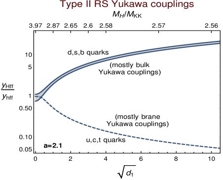
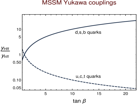
Figure 1: Ratio of Yukawa couplings $\hat{y}_{Hff}/y_{hff}$ in the warped scenario with RS metric (top panel) and in the MSSM (bottom panel). The parameters responsible for splitting the couplings are $\tan\beta$ in the MSSM and $d_{1}$ (the coefficient of the IR-brane localized Higgs kinetic term) in the warped scenario.

In principle there is no reason for the bulk and brane Yukawa coefficients to be of different orders, however, we envision here the case where a relative hierarchy between the two contributions exists.

First we assume that within the up-sector we have $Y_{u}^{bulk}\ll Y_{u}^{brane}$, so that $\delta Y^{u}_{h,H}=\frac{F_{h,H}Y_{u}^{bulk}}{Y_{u}^{brane}}\ll 1$. In that limit we obtain

$$\frac{y_{Hqu}}{y_{hqu}}=\frac{H(y_{1})}{h(y_{1})}\left(1+{\cal O}(\delta Y^{u})\right).$$ (33)

We can further consider the simple limit in which the metric background is the RS metric with the warp factor given by $\sigma(y)=ky$, where $k\approx M_{Pl}$, and the bulk Higgs potential is quadratic in $H$, i.e. we have $V(H)=a(a-4)k^{2}H^{2}$. Here, $a$ is a parameter bound by $a>2$ to ensure that the Higgs VEV, $v(y)\propto e^{aky}$, is sufficiently localized towards the IR brane in order to address the hierarchy problem. In the limit of large Higgs brane kinetic term coefficient, $d_{1}$, we obtain the asymptotic behaviour:

$$\frac{H(y_{1})}{h(y_{1})}\sim\frac{M_{KK}}{M_{H}}\sqrt{\frac{2}{d_{1}}}\ \ \ \ ({\rm large\ d_{1},\ RS\ metric})\,.$$ (34)

Note this relationship is flavour independent as it does not depend on the structure of the 5D bulk mass parameters.

We next assume that for the down-sector quarks, the Yukawa couplings hierarchy is inverted so that $Y_{d}^{bulk}\gg Y_{d}^{brane}$. With the new small parameters $\displaystyle\delta Y^{d}_{h,H}=\frac{Y_{d}^{brane}}{F_{h,H}Y_{d}^{bulk}}\ll 1$ we can again expand the ratio of Yukawa couplings as

$$\frac{y_{Hqd}}{y_{hqd}}=B_{d}(\Delta c)\left(1+{\cal O}(\delta Y^{d})\right)\,,$$ (35)

where we have defined

$$B_{d}(\Delta c)=\frac{\int dye^{(\Delta c)\sigma(y)}H(y)}{\int dye^{(\Delta c)\sigma(y)}h(y)}\,,$$ (36)

and again $\Delta c=c_{u}-c_{q}$. When the background metric is RS and the bulk Higgs potential is quadratic, one could obtain a closed form solution for the integral $B_{d}$ in terms of hypergeometric functions. This solution has been used in Figures 1 and 2. In general, and for large values of $d_{1}$ the Yukawa coupling scales as

$$\frac{y_{Hqd}}{y_{hqd}}\sim\sqrt{d_{1}}\times{\cal O}(1)\ \ \ ({\rm large}\ d_{1}),$$ (37)

which shows the inverse dependence on $d_{1}$ compared to the mostly-brane Yukawa coupling (that we propose for the up-sector). We show the comparison of the warped scenario Yukawa couplings with those of the MSSM in the decoupling limit in Fig. 1, top and bottom panels, respectively.

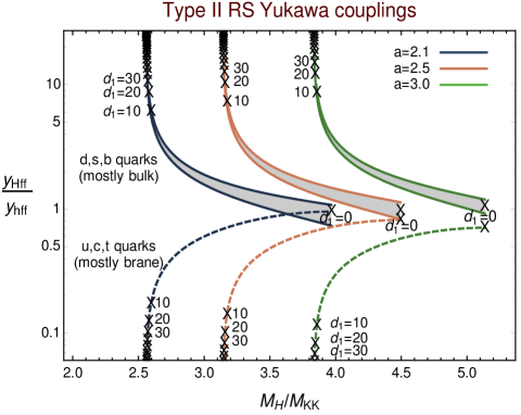
Figure 2: Ratio of Yukawa couplings, $y_{Hff}/y_{hff}$, in the warped scenario with the RS metric. We scan with respect to the heavy Higgs mass $M_{H}$ (relative to the KK scale $M_{KK}$), and show some of the corresponding values of the Higgs brane kinetic term coefficient, $d_{1}$. Three different values of the bulk Higgs mass parameter, $a$, given in the legend at the top right corner, are considered.

It can be shown that to lowest order in $v^{2}/M_{KK}^{2}$, the couplings of the CP-even $H$, the CP-odd $A$, and the charged Higgs $H^{\pm}$ bosons are actually the same (all of these KK excitations originate from the same 5D Higgs doublet and thus their couplings come from the same 5D Yukawa operators). We thus write

$$y_{Hqu}\simeq y_{Aqu}\simeq y_{H^{\pm}qu}\,,$$ (38)

$$y_{Hqd}\simeq y_{Aqd}\simeq y_{H^{\pm}qd}\,,$$ (39)

where $y_{H^{\pm}qu}$ is the coefficient appearing in the coupling between left-handed down quark and right-handed up quark, and $y_{H^{\pm}qd}$ corresponds to left-handed up quark and right-handed down quark. Also note that when the full flavour structure is considered, the heavy Higgs couplings of the warped scenario can involve off-diagonal entries due to a misalignment between the quark mass matrix and the coupling matrix between heavy Higgs bosons and quarks. This effect does not appear within the MSSM as the couplings are simultaneously diagonalized with the quark matrices, and only the charged Higgs couplings involve the CKM entries in a very straightforward way. The collider phenomenology will involve mainly the heavy flavours (top and bottom quarks) so we focus here on these couplings. The ratio of the Yukawa couplings of the top and bottom quarks with the heavy Higgs bosons versus the SM Higgs bosons is plotted in Fig. 2.

The first limit, in which the 5D Yukawa couplings are dominated by the brane Yukawa operator, is interesting because it shows a linear dependence on the value of the wave function of the heavy Higgs at the TeV boundary. This value can be controlled with the Higgs brane kinetic term, which suppresses it for large brane kinetic coefficient, $d_{1}$. This way one can suppress the coupling of the heavy Higgs with up-type fermions, mimicking the behaviour in the MSSM scenario for large $\tan\beta$. For down-type fermions, the Yukawa couplings of the heavy Higgs bosons have a more obscure dependence, but they show a clear enhancement for large brane kinetic coefficient $d_{1}$.

Of course, in general, the warped scenario can have any Yukawa structure. We call the flavour structure in which the up(down)-type fermions have dominant brane(bulk) Yukawa couplings, a Type II Yukawa coupling setup, as it is reminiscent of the Type II 2HDM and the MSSM. Note that other flavour structures are possible in the warped setup and these can easily resemble other types of Yukawa couplings of specific 2HDM’s, such as Type I or flipped Yukawa structures.

6 Discussion and outlook

We have shown that the gauge couplings of heavy exotic Higgs fields in minimal implementations of both supersymmetry and warped extra dimensions are very similar when the masses of the new Higgs bosons are significantly heavier than the electroweak scale and that this is a general result.

We have also shown that the Yukawa couplings of the exotic Higgs bosons can also be very similar in a specific parameter region of the warped extra dimensional model.

The production cross section of neutral Higgs bosons through gluon fusion is governed by their Yukawa couplings. Thus both minimal BSM scenarios analyzed here could yield very similar production rates. The production of charged Higgs bosons will go directly through Yukawa couplings and again we could have very similar production rates in both scenarios.

Once these exotic Higgs bosons are produced they will decay, via gauge (or Yukawa) interactions. Since gauge couplings are similar in both models, it is then quite possible to have a regime in which the whole phenomenology of exotic Higgs bosons is indistinguishable in the two different types of scenarios.

This however does not mean that they have to be always indistinguishable, since the parameter space of warped extra dimensions in the Yukawa sector is much larger. When the Yukawa coupling structure is not governed by hierarchies within brane and bulk Yukawa operators, one would expect both BSM models to be similar only when the top quark coupling to the heavy Higgs bosons dominate over the bottom quark couplings, i.e. in the case of $\tan\beta$ of order 1 in the MSSM.

We have here focused on the simplest metric background for the warped extra-dimensional model. However minimal implementations of the SM within the RS background have strong constraints from precision electroweak tests and flavour phenomenology, and it is known that many of these bounds can be relaxed in the presence of slightly modified metric backgrounds [13], without changing the minimal structure of the Higgs sector. Moreover it was also shown that within these modified scenarios, the heavy Higgs modes can easily have masses well below the masses of the rest of KK excitations of the model [15].

Thus one can perform more realistic phenomenological comparisons of the two models within these new metric scenarios. The disadvantage is that, in that case, analytical expressions for the couplings cannot be obtained in general and one has to rely on numerical computations. The study performed here with the RS metric thus is a preliminary first order study, important in its transparency, and useful for checking the numerical results emerging from a more realistic scenario, which will be the subject of further studies.

7 Aknowlegements

The work of M. F. has been partly supported by NSERC through the grant number SAP105354. M. T. would like to thank FRQNT for financial support under grant number PRC-290000. This paper reflects solely the authors’ personal opinions and does not represent the opinions of the authors’ employers, present and past, in any way.

References

- Aad et al. [2012] G. Aad, et al. (ATLAS), Observation of a new particle in the search for the Standard Model Higgs boson with the ATLAS detector at the LHC, Phys. Lett. B 716 (2012) 1–29. doi:10.1016/j.physletb.2012.08.020. arXiv:1207.7214.
- Chatrchyan et al. [2012] S. Chatrchyan, et al. (CMS), Observation of a New Boson at a Mass of 125 GeV with the CMS Experiment at the LHC, Phys. Lett. B 716 (2012) 30–61. doi:10.1016/j.physletb.2012.08.021. arXiv:1207.7235.
- Lykken [2010] J. D. Lykken, Beyond the Standard Model, in: CERN Yellow Report CERN-2010-002, 101-109, 2010. URL: http://lss.fnal.gov/archive/2010/conf/fermilab-conf-10-103-t.pdf. arXiv:1005.1676.
- Branco et al. [2012] G. C. Branco, P. M. Ferreira, L. Lavoura, M. N. Rebelo, M. Sher, J. P. Silva, Theory and phenomenology of two-Higgs-doublet models, Phys. Rept. 516 (2012) 1–102. doi:10.1016/j.physrep.2012.02.002. arXiv:1106.0034.
- Arcadi et al. [2022] G. Arcadi, A. Djouadi, H.-J. He, J.-L. Kneur, R.-Q. Xiao, The hMSSM with a Light Gaugino/Higgsino Sector:Implications for Collider and Astroparticle Physics (2022). arXiv:2206.11881.
- Djouadi et al. [2013] A. Djouadi, L. Maiani, G. Moreau, A. Polosa, J. Quevillon, V. Riquer, The post-Higgs MSSM scenario: Habemus MSSM?, Eur. Phys. J. C 73 (2013) 2650. doi:10.1140/epjc/s10052-013-2650-0. arXiv:1307.5205.
- Djouadi and Quevillon [2013] A. Djouadi, J. Quevillon, The MSSM Higgs sector at a high : reopening the low tan regime and heavy Higgs searches, JHEP 10 (2013) 028. doi:10.1007/JHEP10(2013)028. arXiv:1304.1787.
- Djouadi et al. [2015] A. Djouadi, L. Maiani, A. Polosa, J. Quevillon, V. Riquer, Fully covering the MSSM Higgs sector at the LHC, JHEP 06 (2015) 168. doi:10.1007/JHEP06(2015)168. arXiv:1502.05653.
- Bagnaschi et al. [2021] E. A. Bagnaschi, S. Heinemeyer, S. Liebler, P. Slavich, M. Spira, Benchmark Scenarios for MSSM Higgs Boson Searches at the LHC (2021).
- Randall and Sundrum [1999] L. Randall, R. Sundrum, A Large mass hierarchy from a small extra dimension, Phys. Rev. Lett. 83 (1999) 3370–3373. doi:10.1103/PhysRevLett.83.3370. arXiv:hep-ph/9905221.
- Burdman [2002] G. Burdman, Constraints on the bulk standard model in the Randall-Sundrum scenario, Phys. Rev. D 66 (2002) 076003. doi:10.1103/PhysRevD.66.076003. arXiv:hep-ph/0205329.
- Agashe et al. [2003] K. Agashe, A. Delgado, M. J. May, R. Sundrum, RS1, custodial isospin and precision tests, JHEP 08 (2003) 050. doi:10.1088/1126-6708/2003/08/050. arXiv:hep-ph/0308036.
- Cabrer et al. [2011] J. A. Cabrer, G. von Gersdorff, M. Quiros, Suppressing Electroweak Precision Observables in 5D Warped Models, JHEP 05 (2011) 083. doi:10.1007/JHEP05(2011)083. arXiv:1103.1388.
- Carena et al. [2003] M. Carena, E. Ponton, T. M. P. Tait, C. E. M. Wagner, Opaque Branes in Warped Backgrounds, Phys. Rev. D 67 (2003) 096006. doi:10.1103/PhysRevD.67.096006. arXiv:hep-ph/0212307.
- Frank et al. [2017] M. Frank, N. Pourtolami, M. Toharia, Bulk Higgs with a heavy diphoton signal, Phys. Rev. D 95 (2017) 036007. doi:10.1103/PhysRevD.95.036007. arXiv:1607.04534.
- Randall and Sundrum [1999] L. Randall, R. Sundrum, An Alternative to compactification, Phys. Rev. Lett. 83 (1999) 4690–4693. doi:10.1103/PhysRevLett.83.4690. arXiv:hep-th/9906064.
- Davoudiasl et al. [2000] H. Davoudiasl, J. L. Hewett, T. G. Rizzo, Bulk gauge fields in the Randall-Sundrum model, Phys. Lett. B 473 (2000) 43–49. doi:10.1016/S0370-2693(99)01430-6. arXiv:hep-ph/9911262.
- Grossman and Neubert [2000] Y. Grossman, M. Neubert, Neutrino masses and mixings in nonfactorizable geometry, Phys. Lett. B 474 (2000) 361–371. doi:10.1016/S0370-2693(00)00054-X. arXiv:hep-ph/9912408.
- Pomarol [2000] A. Pomarol, Gauge bosons in a five-dimensional theory with localized gravity, Phys. Lett. B 486 (2000) 153–157. doi:10.1016/S0370-2693(00)00737-1. arXiv:hep-ph/9911294.
- Agashe et al. [2005] K. Agashe, G. Perez, A. Soni, Flavor structure of warped extra dimension models, Phys. Rev. D 71 (2005) 016002. doi:10.1103/PhysRevD.71.016002. arXiv:hep-ph/0408134.
- Falkowski and Perez-Victoria [2008] A. Falkowski, M. Perez-Victoria, Electroweak Breaking on a Soft Wall, JHEP 12 (2008) 107. doi:10.1088/1126-6708/2008/12/107. arXiv:0806.1737.
- Archer [2012] P. R. Archer, The Fermion Mass Hierarchy in Models with Warped Extra Dimensions and a Bulk Higgs, JHEP 09 (2012) 095. doi:10.1007/JHEP09(2012)095. arXiv:1204.4730.
- Gunion and Haber [2003] J. F. Gunion, H. E. Haber, The CP conserving two Higgs doublet model: The Approach to the decoupling limit, Phys. Rev. D 67 (2003) 075019. doi:10.1103/PhysRevD.67.075019. arXiv:hep-ph/0207010.
- Azatov et al. [2009] A. Azatov, M. Toharia, L. Zhu, Higgs Mediated FCNC’s in Warped Extra Dimensions, Phys. Rev. D 80 (2009) 035016. doi:10.1103/PhysRevD.80.035016. arXiv:0906.1990.