Visual Recognition with Deep Nearest Centroids
Abstract
We devise deep nearest centroids (DNC), a conceptually elegant yet surprisingly ef- fective network for large-scale visual recognition, by revisiting Nearest Centroids, one of the most classic and simple classifiers. Current deep models learn the classi- fier in a fully parametric manner, ignoring the latent data structure and lacking explainability. DNC instead conducts nonparametric, case-based reasoning; it utilizes sub-centroids of training samples to describe class distributions and clearly ex- plains the classification as the proximity of test data to the class sub-centroids in the feature space. Due to the distance-based nature, the network output dimensionality is flexible, and all the learnable parameters are only for data embedding. That means all the knowledge learnt for ImageNet classification can be completely transferred for pixel recognition learning, under the “pre-training and fine-tuning” paradigm. Apart from its nested simplicity and intuitive decision-making mechanism, DNC can even possess ad-hoc explainability when the sub-centroids are selected as ac- tual training images that humans can view and inspect. Compared with parametric counterparts, DNC performs better on image classification (CIFAR-10, CIFAR-100, ImageNet) and greatly boosts pixel recognition (ADE20K, Cityscapes) with improved transparency, using various backbone network architectures (ResNet, Swin) and segmentation models (FCN, DeepLab, Swin). Our code is available at DNC.
1 Introduction
Deep learning models, from convolutional networks (e.g., VGG [1], ResNet [2]) to Transformer-based
architectures (e.g., Swin [3]), push forward the state-of-the-art on visual recognition. With these ad- vancements, parametric softmax classifiers, which learn a set of parameters, i.e., weight vector, and bias term, for each class, have become the de facto regime in the area (Fig. 1(b)). However,
due to the parametric nature, they suffer from several limitations: First, they lack simplicity and explainability. The parameters in the classification layer are abstract and detached from the physical nature of the problem being modelled [4]. Thus these classifiers are hard to naturally lend to an explanation that humans are
able to process [5]. Second, linear classifiers are typically trained to optimize classification accuracy only, paying less attention to modeling the latent data structure. For each class, only one sin- gle weight vector is learned in a fully parametric manner. Thus they essentially assume unimodality for
each class [6, 7], less tolerant of intra-class variation. Third, as each class has its own set of parame-
ters, deep parametric classifiers require the output space with a fixed dimensionality (equal to the number of classes) [8]. As a result, their transferability is limited; when using ImageNet-trained classifiers to initialize segmentation networks (i.e., pixel classifiers), the last classification layer, whose parameters are valuable knowledge learnt from the image classification task, has to be thrown away.
In light of the foregoing discussions, we are motivated to present deep nearest centroids (DNC), a pow- erful, nonparametric classification network (Fig. 1(d)). Nearest Centroids, which has historical roots dating back to the dawn of artificial intelligence [9, 10, 11, 12, 13, 14], is arguably the simplest classifier. Nearest Centroids operates on an intuitive principle: given a data sample, it is directly classified to the class of training examples whose mean (centroid) is closest to it. Apart from its internal transparency, Nearest Centroids is a classical form of exemplar-based reasoning [11, 5], which is fundamental to our most effective strategies for tactical decision-making [15] (Fig. 1(c)). Numerous past studies [16, 17, 18] have shown that humans learn to solve new problems by using past solutions of similar problems. Despite its conceptual simplicity, empirical evidence in cognitive science, and ever popularity [19, 20, 21, 22], Nearest Centroids and its utility in large datasets with high-dimensional input spaces are widely unknown or ignored by current community. Inheriting the intuitive power of Nearest Centroids, our DNC is able to serve as a strong yet interpretable backbone for large-scale visual recognition; it is fully aware of the aforementioned limitations of parametric counterparts while shows even better performance.
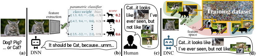
 , built upon parametric softmax classifiers, have a few limitations, such as their non-transparent decision-making process. (c) Humans
  can use past cases as models when solving new problems [16, 18] (e.g., comparing
  with a few familiar/exemplar animals for categorization). (d) DNC
  makes classification based on the similarity of to class sub-centroids (representative training examples) in
the feature space. The class sub-centroids are vital for capturing underlying data structure, enhancing interpretability, and boosting recognition.
makes classification based on the similarity of to class sub-centroids (representative training examples) in
the feature space. The class sub-centroids are vital for capturing underlying data structure, enhancing interpretability, and boosting recognition. Specifically, DNC summarizes each class into a set of sub-centroids (sub-cluster centers) by clustering of training data inside the same class, and assigns each test sample to the class with the nearest sub-centroid.
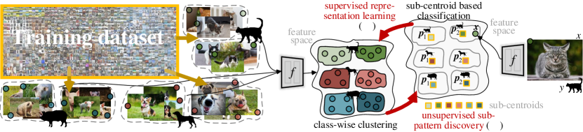
DNC is essentially an experience-/distance-based classifier – it merely relies on the proximity of test query to local means of training data (“quintessential” past observations) in the deep feature space. As such, DNC learns visual recognition by directly optimizing the representation, instead of deep
parametric models needing an extra softmax classification layer after feature extraction. For training, DNC alternates between two steps: i) class-wise clustering for automatically discovering class sub-centroids, and ii) classification prediction for supervised representation learning, through retrieving
the nearest sub-centroids. However, since the feature space evolves continually during training, computing the sub-centroids is expensive – it requires a pass over the full training dataset after each batch update and limits DNC’s scalability. To solve this, we use a Sinkhorn Iteration [23] based clustering algorithm [24] for fast cluster assignment. We further adopt momentum update with an external me- mory for estimating online the sub-centroids (whose amount is more than 1K on ImageNet [25]) with small-batch size (e.g., 256). Consequently, DNC can be efficiently trained by simultaneously conducting clustering and stochastic optimization on large datasets with small batches, only slowing the training speed slightly (e.g., 5% on ImageNet).
DNC enjoys a few attractive qualities: First, improved simplicity and transparency. The intuitive working mechanism and statistical meaning of class sub-centroids make DNC elegant and easy to understand. Second, automated discovery of underlying data structure. By within-class deterministic clustering, the latent distribution of each class is automatically mined and fully captured as a set of representative local means. In contrast, parametric classifiers learn one single weight vector per class, intolerant of rich intra-class variations. Third, direct supervision of representation learning. DNC achieves classification by comparing data samples and class sub-centroids on the feature space. With such distance-based nature, DNC blends unsupervised sub-pattern mining (class-wise clustering) and supervised representation learning (nonparametric classification) in a synergy: local significant pat- terns are automatically mined to facilitate classification decision-making; the supervisory signal from classification directly optimizes the representation, which in turn boosts meaningful clustering. Forth, better transferability. DNC learns by only optimizing the feature representation, thus the output dimensionality no longer needs to be as many as the classes. With this algorithmic merit, all the useful knowledge (parameters) learnt from a source task (e.g., ImageNet [25] classification) are stored in the representation space, and can be completely transferred to target tasks (e.g., Cityscapes [26] segmentation). Fifth, ad-hoc explainability. If further restricting the class sub-centroids to be samples (images) of the training set, DNC can explain its prediction based on IF Then rules and allow users to intuitively view the class representatives, and appreciate the similarity of test data to the representative images (detailed in §3&4.3). Such ad-hoc explainability [27] is valuable in safety-sensitive scenarios, and differs DNC from most existing network interpretation techniques [28, 29, 30] that only investigate post-hoc explanations and thus fail to elucidate precisely how a model works [31, 32].
DNC is an intuitive yet general classification framework; it is compatible with different visual recognition network architectures and tasks. We experimentally show: In §4.1, with ResNet [2] and Swin [3]
network architectures, DNC outperforms parametric counterparts on image classification, i.e., 0.23-0.24% top-1 accuracy on CIFAR-10 [33] and 0.24-0.32% on ImageNet [25], by training from scratch.
In §4.2, when using our ImageNet-pretrained, nonparametric versions of ResNet and Swin as back-
bones, our pixel-wise DNC classifier greatly improves the segmentation performance of FCN [34], DeepLab [35], and UperNet [36], on ADE20K [37] (1.6-2.5% mIoU) and Cityscapes [26] (1.1-1.9% mIoU). These results verify DNC’s strong transferability and high versatility. In §4.3, after con- straining class sub-centroids as training images of ImageNet, DNC becomes more interpretable, with only 0.12% sacrifice in top-1 accuracy (but is still 0.17% better than the parametric counterpart).
These results are particularly impressive, considering the nonparametric and transparent nature of DNC. We feel this work brings fundamental insights into related fields.
2 Related Work
Distance-/Prototype-based Classifiers. Among the numerous classification algorithms (e.g., logistic regression [38], Naïve Bayes [39], random forest [40], support vector machines [41], and deep neural networks (DNNs) [42]), distance-based methods are particularly remarkable, due to their intuitive working mechanism. Distance-based classifiers are nonparametric and exemplar-driven, relying on similarities between samples and internally stored exemplars/prototypes. Thus they conduct case-based reasoning that humans use naturally in problem-solving, making them appealing and interpretable [16, 43]. -Nearest Neighbors (-NN) [9, 10] is a form of distance-based classifiers; it uses all training data as exemplars [44, 45]. Towards network implementation of -NN [46, 47, 48], Wu et al. [49] made notable progress; their -NN network outperforms parametric softmax based ResNet [2] and the learnt representation works well in few-shot settings. However, -NN classifiers (including the deep learning analogues) cost huge storage space and pose heavy computation burden (e.g., persistently retaining the training dataset and making full-dataset retrieval for each query) [50, 51], and the nearest neighbors may not be good class representatives [43]. Nearest Centroids [11, 12, 13, 14] is another famous distance-based classifier yet has neither of the deficiencies of -NN [20, 43]. Nearest Centroids selects representative class centers, instead of all the training data, as exemplars. Guerriero et al. [52] also investigate the idea of bringing Nearest Centroids into DNNs. However, they simply abstract each class into one single class mean, failing to capture complex class-wise distributions and showing weak results even in small datasets [33].
The idea of distance-based classification also stimulates the emergence of prototypical networks, which mainly focus on few-shot [53, 54] and zero-shot [55, 56] learning. However, they often associate to each class only one representation (prototype) [57] and their prototypes are usually flexible parameters [53, 51, 56] or defined prior to training [55, 8]. In DNC, a prototype (sub-centroid) is either a generalization of a number of observations or intuitively a typical training visual example. Via clustering based sub-class mining, DNC addresses two key properties of prototypical exemplars: sparsity and expressivity [58, 59]. In this way, the representation can be learnt to capture the underlying class structure, hence facilitating large-scale visual recognition while preserving transparency.
Neural Network Interpretability. As the black-box nature limits the adoption of DNNs in decision-critical tasks, there has been a recent surge of interest in DNNs’ interpretability. However, most interpretation techniques only produce posteriori explanations for already-trained DNNs, typically by analysis of reverse-engineer importance values [60, 28, 29, 61, 62, 63, 30, 64, 65] and sensitivities of inputs [66, 67, 68, 69]. As many literature outlined, post-hoc explanations are problematic and misleading [70, 32, 71, 43]; they cannot explain what actually makes a DNN arrive at its decisions [72]. To pursue ad-hoc explainability, some attempts have been initiated to develop explainable DNNs, by deploying more interpretable machineries into black-box DNNs [73, 74, 75] or regularizing representation with certain properties (e.g., sparsity [76], decomposability [77], monotonicity [78]) that can enhance interpretability.
DNC intrinsically relies on class sub-centroid retrieving. The theoretical simplicity makes it easy to understand; when anchoring the sub-centroids to available observations, DNC can derive intuitive explanations based on the similarities of test samples to representative observations. It simultaneously conducts representation learning and case-based reasoning, making it self-explainable without post-hoc analysis [27]. DNC relates to concept-based explainable networks [73, 5, 74, 79, 72, 80, 4, 81] that
refer to human-friendly concepts/prototypes during decision making. These methods, however, necessitate nontrivial architectural modification and usually resort to pre-trained models, not to men- tion serving as backbone networks. In sharp contrast, DNC only brings minimal architectural change to parametric classifier based DNNs and yields remarkable performance on ImageNet [25] with training from scratch and ad-hoc explainability. It provides solid empirical evidence, for the first time as far as we know, for the power of case-based reasoning in large-scale visual recognition.
3 Deep Nearest Centroids (DNC)
Problem Statement. Consider the standard visual recognition setting. Let be the visual space (e.g., image space for recognition, pixel space for segmentation), and the set of semantic classes. Given a training dataset , the goal is to use the training examples to fit a model (or hypothesis) that accurately predicts the semantic classes for new visual samples.
Parametric Softmax Classifier. Current common practice is to implement as DNNs and decompose it as . Here is a feature extractor (e.g., convolution based or Transformer-like networks) that maps an input sample into a -dimensional representation space , i.e., ; and is a parametric classifier (e.g., the last fully-connected layer in recognition or last 11 convolution layer in segmentation) that takes as input and produces class prediction . Concretely, assigns a query to the class according to:
| (1) |
where indicates the unnormalized prediction score (i.e., logit) for class , and are learnable parameters – class weight and bias term for . Parameters of and are learnt by mini- mizing the softmax cross-entropy loss:
| (2) |
Though highly successful, the use of the parametric classifier has drawbacks as well: i) The weight matrix and bias vector in are learnable parameters, which cannot provide any information about what makes the model reach its decisions. ii) makes the loss only depend on the relative relation among logits, i.e., , and cannot directly supervise on the representation [82, 83]. iii) and are learnt as flexible parameters, lacking explicit modeling of the underlying data structure. iv) The final output dimensionality is constrained to be the number of classes, i.e., . During transfer learning, as different visual recognition tasks typically have distinct semantic label spaces (with different number of classes), the classifier from a pretrained model has to be abandoned, even though the learnt parameters and are valuable knowledge from the source task.
The question naturally arises: might there be a simple way to address these limitations of current de facto, parametric classifier based visual recognition regime? Here we show that this is indeed possible, even with better performance.
DNC Classifier. Our DNC (Fig. 2) is built upon the intuitive idea of Nearest Centroids, i.e., assign a sample to the class with the closest class center:
| (3) |
where is a distance measure, given as: . For simplicity, all the features are defaulted to -normalized from now on. is the mean vector of class , is a training sample of , i.e., , and is the number of training samples in . As such, the feature-to-class mapping is achieved in a nonparametric manner and understandable from user’s view, in contrast to the parametric classifier that learns “non-transparent” parameters for each class. It makes more sense if multiple sub-centroids (local means) per class are used, which is in particular true for challenging visual recognition where complex intra-class variations cannot be simply described by the simple assumption of unimodality of data of each class. When representing each class as sub-centroids, denoted by , the -way classification for sample takes place as a winner-takes-all rule:
| (4) |
Clearly, estimating class sub-centroids needs clustering of training samples within each class. As class
sub-centroids are sub-cluster centers in the latent feature space , they are locally significant visual patterns and can comprehensively represent class-level characteristics. DNC can be intuitively understood as selecting and storing prototypical exemplars for each class, and finding classification evidence for a previously unseen sample by retrieving the most similar exemplar. This also aligns with the prototype theory in psychology [17, 84, 85]: prototypes are a typical form of cognitive organisation of real world objects. DNC thus emulates the case-based reasoning process that we humans are accustomed to [27]. For instance, when ornithologists classify a bird, they will compare it with those typical exemplars from known bird species to decide which species the bird belongs to [43].
Sub-centroid Estimation. To find informative sub-centroids that best represent classes, we perform deterministic clustering within each class on the representation space . More specifically, for each class , we cluster all the representations into clusters whose centers are used as the sub-centroids of , i.e., . Let and denote the feature and sub-centroid matrixes, respectively. The deterministic clustering, i.e., the mapping from to , can be denoted as , where -th column is an one-hot assignment vector of -th sample w.r.t the clusters. is desired to maximize the similarity between and , leading to the following binary integer program (BIP):
| (5) |
where is a -dimensional all-ones vector. As in [24], we relax to be a transportation polytope [23]: , casting BIP (5) into an optimal transport problem. In , besides the one-hot assignment constraint (i.e., ), an equipartition constraint (i.e., ) is added to inspire samples to be evenly assigned to clusters. This can efficiently avoid degeneracy, i.e., mapping all the data to the same cluster. Then the solution can be given by a fast version [23] of Sinkhorn-Knopp algorithm [86], in a form of a normalized exponential matrix:
| (6) |
where the exponentiation is performed element-wise, and are two renormalization vectors, which can be computed using a small number of matrix multiplications via Sinkhorn-Knopp Iteration [23], and trades off convergence speed with closeness to the original transport problem. In short, by mapping data samples into a few clusters under the constraints , we pursue sparsity and expressivity [58, 59], making class sub-centroids representative of the dataset.
Training of DNC = Supervised Representation Learning + Automatic Sub-class Pattern Mining. Ideally, according to class-wise cluster assignments , we can get totally sub-centroids , i.e., mean feature vectors of the training data in the clusters. Then the training target becomes as:
| (7) |
Comparing (2) and (7), as the class sub-centroids are derived solely from data representations, DNC learns visual recognition by directly optimizing the representation , instead of the parametric classifier . Moreover, with such a nonparametric, distance-based scheme, DNC builds a closer link to metric learning [87, 88, 89, 90, 91, 92, 93]; DNC can even be viewed as learning a metric function to compare data samples , under the guidance of the corresponding semantic labels .
During training, DNC alternates two steps iteratively: i) class-wise clustering (5) for automatic sub-centroid discovery, and ii) sub-centroid based classification for supervised representation learning (7). Through clustering, DNC probes underlying data distribution of each class, and produces informative sub-centroids by aggregating statistics from data clusters. This automatic sub-class discovery process also enjoys a similar spirit of recent clustering based unsupervised representation learning [94, 95, 96, 97, 98, 99, 24, 100, 101]. However, it works in a class-wise manner, since the class label is given. In this way, DNC opti- mizes the representation by adjusting the arrangement between sub-centroids and data samples. The enhanced representation in turn helps to find more informative sub-centroids, benefiting classification eventually. As such, DNC conducts unsupervised sub-class pattern discovery during supervised representation learning, distinguishing it from most (if not all) of current visual recognition models.
Since the latent representation evolves continually during training, class sub-centroids should be synchronized, which requires performing class-wise clustering over all training data after each batch
update. This is highly expensive on large datasets, even though Sinkhorn-Knopp iteration [23] based clustering (6) is highly efficient. To circumvent the expensive, offline sub-centroid estimation, we adopt momentum update and online clustering. Specifically, at each training iteration, we conduct class-wise clustering on the current batch and update each sub-centroid as:
| (8) |
where is a momentum coefficient, and is the mean feature vector of data assigned to -cluster in current batch. As such, the sub-centroids can be up-to-date with the change of para- meters. Though effective enough in most cases, batch-wise clustering could not extend to a large num- ber of classes, e.g., when training on ImageNet [25] with 1K classes using batch size 256, not all the classes/clusters are present in a batch. To solve this, we store features from several prior batches in a memory, and do clustering on both the memory and current batch. DNC can be trained by gradient backpropagation in small-batch setting, with negligible lagging (5% training delay on ImageNet).
Versatility. DNC is a general framework; it can be effortless integrated into any parametric classifier based DNNs, with minimal architecture change, i.e., removing the parametric softmax layer. However, DNC changes the classification decision-making mode, reforms the training regime, and makes the reasoning process more transparent, without slowing the inference speed. DNC can be ap- plied to various visual recognition tasks, including image classification (§4.1) and segmentation (§4.2).
Transferability. As a nonparametric scheme, DNC can handle an arbitrary number of classes with fixed output dimensionality (); all the knowledge learnt on a source task (e.g., ImageNet classification with 1K classes) are stored as a constant amount of parameters in , and thus can be completely transferred for a new task (e.g., Cityscapes [26] segmentation with 19 classes), under the “pre-training and fine-tuning” paradigm. In a similar setting, the parametric counterpart has to discard 2M parameters during transfer learning ( when using ResNet101 [2]). See §4.2 for related experiments.
Ad-hoc Explainability. DNC is a transparent classifier that has a built-in case-based reasoning process, as the sub-centroids are summarized from real observations and actually used during classification. So far we only discussed the case where the sub-centroids are considered as average mean feature vectors of a few training samples with similar patterns. When restricting the sub-centroids to be elements of the training set (i.e., representative training images), DNC naturally comes with human-understandable explanations for each prediction, and the explanations are loyal to the inter- nal decision mode and not created post-hoc. Studies regarding ad-hoc explainability are given in §4.3.
4 Experiment
4.1 Experiments on Image Classification
Dataset. The evaluation for image classification is carried out on CIFAR-10 [33] and ImageNet [25].
Network Architecture. For completeness, we craft DNC on popular CNN-based ResNet50/100 [2] and recent Transformer-based Swin-Small/-Base [3]. Note that, we only remove the last linear classification layer, and the final output dimensionality of DNC is as many as the last layer feature of the parametric counterpart, i.e., 2,048 for ResNet50/100, 768 for Swin-Small, and 1,024 for Swin-Base.
Training. We use mmclassification111https://github.com/open-mmlab/mmclassification as codebase and follow the default training settings. For CIFAR-10, we train ResNet for epochs, with batch size . The memory size for DNC models is set as 100 batches. For ImageNet, we train 100 and 300 epochs with batch size for ResNet and Swin, respectively. The initial learning rates of ResNet and Swin are set as and , scheduled by a step policy and polynomial annealing policy, respectively. Limited by our GPU capacity, the memory sizes are set as and batches for DNC versions of ResNet and Swin, respectively. Other hyper-
parameters are empirically set as: and . Models are trained from scratch on eight V100 GPUs.
Results on CIFAR-10. Table 1 compares DNC with the parametric counterpart, based on the most repre- sentative CNN network architecture, i.e., ResNet. As seen, DNC obtains better performance: DNC is 0.23% higher on ResNet50, and 0.24% higher on ResNet101, using fewer learnable parameters. With the exact same backbone architectures and training settings, one can safely attribute the performance gain to DNC.
| Method | Backbone | #Params | top-1 | top-5 |
|---|---|---|---|---|
| ResNet [2] | ResNet50 | 25.56M | 76.20% | 93.01% |
| DNC-ResNet | 23.51M | 76.49% | 93.08% | |
| ResNet [2] | ResNet101 | 44.55M | 77.52% | 93.06% |
| DNC-ResNet | 42.50M | 77.80% | 93.85% | |
| Swin [3] | Swin-S | 49.61M | 83.02% | 96.29% |
| DNC-Swin | 48.84M | 83.26% | 96.40% | |
| Swin [3] | Swin-B | 87.77M | 83.36% | 96.44% |
| DNC-Swin | 86.75M | 83.68% | 97.02% |
Results on ImageNet. Table 2 illustrates again our compelling results over different vision net- work architectures. In terms of top-1 acc., our
DNC exceeds the parametric classifier by 0.29% and 0.28%
on ResNet50 and ResNet101, respec- tively. DNC also obtains promising results with Transformer architecture: 83.26% vs 83.02% on Swin-S, 83.68% vs 83.36% on Swin-B. These results are impressive, considering the transpa- rent, case-based reasoning nature of DNC. One may notice another nonparametric, -NN classi- fier [49] reports 76.57% top-1 acc., based on ResNet50. However, [49] is trained with 130 epochs; in
this setting, DNC gains 76.64%. Moreover, as mentioned in §2, [49] poses huge storage demand, i.e., retaining the whole ImageNet training set (i.e., 1.2M images) to perform the -NN decision rule, and suffers from very low efficiency, caused by extensive comparisons between each test image and all the training images. These limitations prevent the adoption of [49] in real application scenarios. In contrast, DNC only relies on a small set of class representatives (i.e., four sub-centroids per class) for
classification decision-making and causes no extra computation budget during network deployment.
4.2 Experiments on Semantic Segmentation
Dataset. The evaluation for semantic segmentation is carried out on ADE20K [37] and Cityscapes [26].
Segmentation Network Architecture. For comprehensive evaluation, we approach DNC on three famous segmentation models (i.e., FCN [34], DeepLab [35], UperNet [36]), using two backbone architectures (i.e., ResNet101 [2] and Swin-B [3]). For the segmentation models, the only architec- tural modification is the removal of the “segmentation head” (i.e., conv based, pixel-wise classi- fication layer). For the backbone networks, we respectively adopt parametric classifier based and our nonparametric, DNC based versions, which are both trained on ImageNet [25] and reported in Table 2, for initialization. Thus for each segmentation model, we derive four variants from the different combinations of parametric and DNC versions of the backbone and segmentation network architectures.
Training. We adopt mmsegmentation222https://github.com/open-mmlab/mmsegmentation as the codebase, and follow the default training settings.
We train FCN and DeepLab with ResNet101 using SGD optimizer with an initial learning rate , and UperNet with Swin-B using AdamW with an initial learning rate 6e-5. For all the models, the learning rate is scheduled following a polynomial annealing policy. As common practices [102, 103], we train the models on ADE20K train with crop size and batch size ; on Cityscapes train with crop size and batch size . All the models are trained for K iterations on
both datasets. Standard data augmentation techniques are used, including scale and color jittering, flipping, and cropping. The hyper-parameters of DNC are by default set as: and .
| ImageNet | ADE20K | Cityscapes | |||
|---|---|---|---|---|---|
| Method | Backbone | top-1 acc. | #Params | mIoU | mIoU |
| ResNet101 [2] | 77.52% | 68.6M | 39.9% | 75.6% | |
| FCN [34] | DNC-ResNet101 | 77.80% | 68.6M | 40.4%0.5 | 76.3%0.7 |
| ResNet101 [2] | 77.52% | 68.5M | 41.1%1.2 | 76.7%1.1 | |
| DNC-FCN | DNC-ResNet101 | 77.80% | 68.5M | 42.3%2.4 | 77.5%1.9 |
| ResNet101 [2] | 77.52% | 62.7M | 44.1% | 78.1% | |
| DeepLab [35] | DNC-ResNet101 | 77.80% | 62.7M | 44.6%0.5 | 78.7%0.6 |
| ResNet101 [2] | 77.52% | 62.6M | 45.0%0.9 | 79.1%1.0 | |
| DNC-DeepLab | DNC-ResNet101 | 77.80% | 62.6M | 45.7%1.6 | 79.8%1.7 |
| Swin-B [3] | 83.36% | 90.6M | 48.0% | 79.8% | |
| UperNet [36] | DNC-Swin-B | 83.68% | 90.6M | 48.4%0.4 | 80.1%0.3 |
| Swin-B [3] | 83.36% | 90.5M | 48.6%0.6 | 80.5%0.7 | |
| DNC-UperNet | DNC-Swin-B | 83.68% | 90.5M | 50.5%2.5 | 80.9%1.1 |
Performance on Segmentation. As summarized in Table 3, our DNC seg- mentation models, no matter whether using DNC based backbones, obtain better performance over parametric competitors, i.e., FCN + ResNet101, DeepLab + ResNet101, UperNet + Swin-B, across different segmentation and backbone network architectures. Taking as an example the famous FCN, the original version gains 39.91% and 75.6% mIoU on ADE20K and City- scapes, respectively. By comparison, with the same backbone – ResNet101, DNC-FCN boosts the scores to 41.1% and 76.7%. When turning to DNC pre-trained backbone – DNC-ResNet101, our DNC-FCN outperforms again its parametric counterpart – FCN, i.e., 42.3% vs 40.4% on ADE20K, 77.5% vs 76.3% on Cityscapes. Similar trends can be also observed for DeepLab and UperNet.
Analysis on Transferability. One appealing feature of DNC is its strong transferability, as DNC learns classification by directly comparing data samples in the feature space. The results in Table 3
also evidence this point. For example,
DeepLab – even a parametric classifier based segmentation model – can
achieve large performance gains, i.e., 44.6% vs 44.1% on ADE20K,
78.7% vs 78.1% on Cityscapes, after using DNC-ResNet101 for fine-tuning. When it comes to DNC-DeepLab, better performance can be achieved, after replacing ResNet101 with DNC-ResNet101,
i.e., 45.7% vs 45.0% on ADE20K, 79.8% vs 79.1% on Cityscapes. We speculate this is because, when the segmentation and backbone networks are both built upon DNC, the model only needs to adapt the original representation space to the target task, without learning any extra new parameters. Also, these impressive results reflect the innovative opportunity of applying our DNC for more downstream visual recognition tasks, either as a new classification network architecture or a strong and transferable backbone.
4.3 Study of Ad-hoc Explainability
So far, we have empirically showed that, by inheriting the intuitive power of Nearest Centroids and the strong representation learning ability of DNNs, DNC can
serve as a transparent yet powerful tool for visual recognition tasks with improved transferability.
When anchoring the class sub-centroids to
real observations (i.e., actual images from the training dataset), instead of selecting them as cluster centers (i.e., mean features of a set of training images), one may expect that DNC will gain enhanced ad-hoc explainability. Next we will show this is indeed possible, only at negligible performance cost.
Experimental Setup. We still train DNC version of ResNet50 on ImageNet train for 100 epochs. In the first 90 epochs, the model is trained in a standard manner, i.e., computing the class sub-centroids as cluster centers. Then we anchor each sub-centroid to its closest training image, based on the co- sine similarity of features. In the final 10 epochs, the sub-centroids are only updated as the features
![[Uncaptioned image]](/html/2209.07383/assets/x3.png)
of their anchored training images. Besides this, all the other training settings are as normal. In this way, we can get a more interpretable DNC-ResNet50.
Interpretable Class Sub- centroids. The top of Fig. 3 plots our discovered sub-centroid images for four ImageNet classes. These representative images are diverse in appearance, viewpoints, illuminations, scales, etc., characterizing their corresponding classes and allowing humans to view and understand.
| Sub-centroid | Architecture | top-1 | top-5 |
|---|---|---|---|
| cluster center | DNC-ResNet50 | 76.49% | 93.08% |
| real observation | 76.37% | 93.04% | |
| - | ResNet50[2] | 76.20% | 93.01% |
Performance with Improved Interpretability. We then report the score of our DNC-ResNet50 based on the interpretable class representatives on Image- Net val. As shown in Table 4, enforcing the class sub-centroids as real training images only brings marginal performance degradation (e.g., 76.49% 76.37% top-1 acc.), while coming with better in- terpretability. More impressively, our explainable DNC-ResNet50 even outperforms the vanilla black-box ResNet50, e.g., 76.37% vs 76.20%.
Explain Inner Decision-Making Mode based on IF Then Rules. With the simple Nearest Cen- troids mechanism, we can use the representative images to form a set of IF Then rules [4], so as to intuitively interpret the inner decision-making mode of DNC for human users. In particular, let denote a sub-centroid image for class , representative images for all the other classes, and a query image. One linguistic logical IF Then rule can be generated for :
| (9) |
where stands for similarity, given by DNC. The final rule for class is created by combining all the rules of sub-centroid images of class (see Fig. 3 bottom):
| IF | (10) | |||
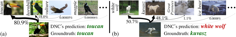
Interpret Prediction Based on (Dis)similarity to Sub-centroid Images. Based on the interpretable class representatives, DNC can explain its predictions by letting users view and verify its computed (dis)similarity between query and class sub-centroid images. As shown in Fig. 4(a), an observation is correctly classified, as DNC thinks it looks (more) like a particular exemplar of “toucan”. However, in Fig. 4(b), DNC struggles to assign the observation to two exemplars from “white wolf” and “kuvasz” respectively, and makes a wrong decision finally. Though users are unclear how DNC maps an image to feature, they can easily understand the decision-making mode [43] (e.g., why is one class predicted over another), and verify the calculated (dis)similarity – the evidence for classification decision.
4.4 Diagnostic Experiment
To perform extensive ablation experiments, we train ResNet101 classification and DeepLab seg- mentation models for epochs and K iterations, on ImageNet and ADE20K, respectively.
Class Sub-centroids. Table 5(a) studies the impact of the number of class sub-centroids () for each class. When , each class is represented by its centroid – the average feature vector of all the training samples of the class (Eq. 3), without clustering. The corresponding baseline obtains top-1 acc. and mIoU for classification and segmentation, respectively. For classification, increasing from 1 to 4 leads to better performance (i.e., ). This supports our hypothesis that one single class weight/center is far from enough to capture the underlying data distribution and proves the efficacy of our clustering based sub-class pattern mining. We stop using as the required memory exceeds the computational limit of our hardware. We find similar trends on segmentation; using more sub-centroids () brings noticeable performance boost: 43.2% 44.3%. However, increasing above 10 provides marginal or even negative gain. This may be because over-clustering finds some insignificant patterns, which are trivial or harmful for decision-making.
External Memory. We next study the influence of the external memory, only used in image classification. As shown in Table 5(b), DNC gradually improves the performance as the increase of the memory size. It reaches top-1 acc. at size . However, the results are still not reaching the performance saturating point, but rather the upper limit of our hardware’s computational budget.
| ImageNet | ADE20K | |||
|---|---|---|---|---|
| top-1 | top-5 | mIoU | ||
| 1 | 77.31 | 93.01 | 1 | 43.2 |
| 2 | 77.54 | 93.32 | 5 | 44.0 |
| 3 | 77.68 | 93.63 | 10 | 44.3 |
| 4 | 77.80 | 93.85 | 20 | 44.0 |
| Memory | ImageNet | |
|---|---|---|
| (#batch) | top-1 | top-5 |
| 0 | 77.49 | 93.09 |
| 700 | 77.58 | 93.16 |
| 800 | 77.64 | 93.35 |
| 900 | 77.75 | 93.67 |
| 1000 | 77.80 | 93.85 |
| ImageNet | ADE20K | ||
| top-1 | top-5 | mIoU | |
| 73.82 | 93.02 | 42.7 | |
| 76.41 | 93.07 | 43.6 | |
| 77.33 | 93.51 | 44.0 | |
| 0.999 | 77.80 | 93.85 | 44.3 |
| 77.31 | 93.48 | 44.2 | |
Momentum Update. Last, we ablate the effect of the momentum coefficient (Eq. 8) that controls the speed of sub-centroid online updating. From Table 5(c) we find the behaviors of are consistent in both tasks. In particular, DNC performs well with larger coefficients (i.e., ), signifying the importance of slow updating. The performance degrades when , and encounters a large drop when (i.e., only using batch sub-centroids as approximations).
5 Conclusion
We present deep nearest centroids (DNC), building upon the classic idea of classifying data samples according to nonparametric class representatives. Compared to classic parametric models, DNC has merits in: i) systemic simplicity by bringing the intuitive Nearest Centroids mechanism to DNNs; ii) automated discovery of latent data structure using within-class clustering; iii) direct supervision of representation learning, boosted by unsupervised sub-pattern mining; iv) improved transferability that lossless transfers learnable knowledge across tasks; and v) ad-hoc explainability by anchoring class exemplars with real observations. Experiments confirm the efficacy and enhanced interpretability.
Acknowledgement
This research was supported by the National Science Foundation under Grant No. 2242243.
References
- [1] Simonyan, K., Zisserman, A.: Very deep convolutional networks for large-scale image recognition. In: ICLR (2015)
- [2] He, K., Zhang, X., Ren, S., Sun, J.: Deep residual learning for image recognition. In: CVPR (2016)
- [3] Liu, Z., Lin, Y., Cao, Y., Hu, H., Wei, Y., Zhang, Z., Lin, S., Guo, B.: Swin transformer: Hierarchical vision transformer using shifted windows. In: ICCV (2021)
- [4] Angelov, P., Soares, E.: Towards explainable deep neural networks (xdnn). Neural Networks 130, 185–194 (2020)
- [5] Li, O., Liu, H., Chen, C., Rudin, C.: Deep learning for case-based reasoning through prototypes: A neural network that explains its predictions. In: AAAI (2018)
- [6] Hayashi, H., Uchida, S.: A discriminative gaussian mixture model with sparsity. In: ICLR (2021)
- [7] Zhou, T., Wang, W., Konukoglu, E., Van Gool, L.: Rethinking semantic segmentation: A prototype view. In: CVPR (2022)
- [8] Mettes, P., van der Pol, E., Snoek, C.: Hyperspherical prototype networks. In: NeurIPS (2019)
- [9] Fix, E., Hodges Jr, J.L.: Discriminatory analysis - nonparametric discrimination: Small sample performance. Tech. rep., California Univ Berkeley (1952)
- [10] Cover, T., Hart, P.: Nearest neighbor pattern classification. IEEE TIT 13(1), 21–27 (1967)
- [11] Kolodner, J.L.: An introduction to case-based reasoning. Artificial Intelligence Review 6(1), 3–34 (1992)
- [12] Kohonen, T.: Learning vector quantization. In: Self-Organizing Maps, pp. 175–189 (1995)
- [13] Chaudhuri, B.: A new definition of neighborhood of a point in multi-dimensional space. Pattern Recognition Letters 17(1), 11–17 (1996)
- [14] Webb, A.R.: Statistical pattern recognition. John Wiley & Sons (2003)
- [15] Kim, B., Rudin, C., Shah, J.A.: The bayesian case model: A generative approach for case-based reasoning and prototype classification. In: NeurIPS (2014)
- [16] Newell, A., Simon, H.A., et al.: Human problem solving, vol. 104 (1972)
- [17] Rosch, E.H.: Natural categories. Cognitive Psychology 4(3), 328–350 (1973)
- [18] Aamodt, A., Plaza, E.: Case-based reasoning: Foundational issues, methodological variations, and system approaches. AI Communications 7(1), 39–59 (1994)
- [19] Slade, S.: Case-based reasoning: A research paradigm. AI magazine 12(1), 42–42 (1991)
- [20] Sánchez, J.S., Pla, F., Ferri, F.J.: On the use of neighbourhood-based non-parametric classifiers. Pattern Recognition Letters 18(11-13), 1179–1186 (1997)
- [21] Gou, J., Yi, Z., Du, L., Xiong, T.: A local mean-based k-nearest centroid neighbor classifier. The Computer Journal 55(9), 1058–1071 (2012)
- [22] Mensink, T., Verbeek, J., Perronnin, F., Csurka, G.: Distance-based image classification: Generalizing to new classes at near-zero cost. IEEE TPAMI 35(11), 2624–2637 (2013)
- [23] Cuturi, M.: Sinkhorn distances: Lightspeed computation of optimal transport. In: NeurIPS (2013)
- [24] Asano, Y.M., Rupprecht, C., Vedaldi, A.: Self-labelling via simultaneous clustering and representation learning. In: ICLR (2020)
- [25] Russakovsky, O., Deng, J., Su, H., Krause, J., Satheesh, S., Ma, S., Huang, Z., Karpathy, A., Khosla, A., Bernstein, M.S., Berg, A.C., Li, F.: Imagenet large scale visual recognition challenge. IJCV 115(3), 211–252 (2015)
- [26] Cordts, M., Omran, M., Ramos, S., Rehfeld, T., Enzweiler, M., Benenson, R., Franke, U., Roth, S., Schiele, B.: The cityscapes dataset for semantic urban scene understanding. In: CVPR (2016)
- [27] Biehl, M., Hammer, B., Villmann, T.: Prototype-based models in machine learning. Wiley Interdisciplinary Reviews: Cognitive Science 7(2), 92–111 (2016)
- [28] Simonyan, K., Vedaldi, A., Zisserman, A.: Deep inside convolutional networks: Visualising image classification models and saliency maps. arXiv preprint arXiv:1312.6034 (2013)
- [29] Zeiler, M.D., Fergus, R.: Visualizing and understanding convolutional networks. In: ECCV (2014)
- [30] Zhou, B., Khosla, A., Lapedriza, A., Oliva, A., Torralba, A.: Learning deep features for discriminative localization. In: CVPR (2016)
- [31] Lipton, Z.C.: The mythos of model interpretability: In machine learning, the concept of interpretability is both important and slippery. Queue 16(3), 31–57 (2018)
- [32] Rudin, C.: Stop explaining black box machine learning models for high stakes decisions and use interpretable models instead. Nature Machine Intelligence 1(5), 206–215 (2019)
- [33] Krizhevsky, A., Hinton, G.: Learning multiple layers of features from tiny images. Technical report, University of Toronto (2009)
- [34] Long, J., Shelhamer, E., Darrell, T.: Fully convolutional networks for semantic segmentation. In: CVPR (2015)
- [35] Chen, L.C., Papandreou, G., Schroff, F., Adam, H.: Rethinking atrous convolution for semantic image segmentation. arXiv preprint arXiv:1706.05587 (2017)
- [36] Xiao, T., Liu, Y., Zhou, B., Jiang, Y., Sun, J.: Unified perceptual parsing for scene understanding. In: ECCV (2018)
- [37] Zhou, B., Zhao, H., Puig, X., Fidler, S., Barriuso, A., Torralba, A.: Scene parsing through ade20k dataset. In: CVPR (2017)
- [38] Friedman, J.H.: The elements of statistical learning: Data mining, inference, and prediction. Springer (2009)
- [39] Hand, D.J., Yu, K.: Idiot’s bayes—not so stupid after all? International Statistical Review 69(3), 385–398 (2001)
- [40] Breiman, L.: Random forests. Machine Learning 45(1), 5–32 (2001)
- [41] Cortes, C., Vapnik, V.: Support-vector networks. Machine Learning 20(3), 273–297 (1995)
- [42] LeCun, Y., Bengio, Y., Hinton, G.: Deep learning. nature 521(7553), 436–444 (2015)
- [43] Rudin, C., Chen, C., Chen, Z., Huang, H., Semenova, L., Zhong, C.: Interpretable machine learning: Fundamental principles and 10 grand challenges. Statistics Surveys 16, 1–85 (2022)
- [44] Boiman, O., Shechtman, E., Irani, M.: In defense of nearest-neighbor based image classification. In: CVPR (2008)
- [45] Guillaumin, M., Mensink, T., Verbeek, J., Schmid, C.: Tagprop: Discriminative metric learning in nearest neighbor models for image auto-annotation. In: ICCV (2009)
- [46] Lippmann, R.P.: Pattern classification using neural networks. IEEE Communications Magazine 27(11), 47–50 (1989)
- [47] Salakhutdinov, R., Hinton, G.: Learning a nonlinear embedding by preserving class neighbourhood structure. In: Artificial Intelligence and Statistics. pp. 412–419 (2007)
- [48] Papernot, N., McDaniel, P.: Deep k-nearest neighbors: Towards confident, interpretable and robust deep learning. arXiv preprint arXiv:1803.04765 (2018)
- [49] Wu, Z., Efros, A.A., Yu, S.X.: Improving generalization via scalable neighborhood component analysis. In: ECCV (2018)
- [50] Garcia, S., Derrac, J., Cano, J., Herrera, F.: Prototype selection for nearest neighbor classification: Taxonomy and empirical study. IEEE TPAMI 34(3), 417–435 (2012)
- [51] Yang, H.M., Zhang, X.Y., Yin, F., Liu, C.L.: Robust classification with convolutional prototype learning. In: CVPR (2018)
- [52] Guerriero, S., Caputo, B., Mensink, T.: Deepncm: Deep nearest class mean classifiers. In: ICLR workshop (2018)
- [53] Snell, J., Swersky, K., Zemel, R.S.: Prototypical networks for few-shot learning. In: NeurIPS (2017)
- [54] Dong, N., Xing, E.P.: Few-shot semantic segmentation with prototype learning. In: BMVC (2018)
- [55] Jetley, S., Romera-Paredes, B., Jayasumana, S., Torr, P.: Prototypical priors: From improving classification to zero-shot learning. arXiv preprint arXiv:1512.01192 (2015)
- [56] Xu, W., Xian, Y., Wang, J., Schiele, B., Akata, Z.: Attribute prototype network for zero-shot learning. In: NeurIPS (2020)
- [57] Rebuffi, S.A., Kolesnikov, A., Sperl, G., Lampert, C.H.: icarl: Incremental classifier and representation learning. In: CVPR (2017)
- [58] Quattoni, A., Collins, M., Darrell, T.: Transfer learning for image classification with sparse prototype representations. In: CVPR (2008)
- [59] Biehl, M., Hammer, B., Schneider, P., Villmann, T.: Metric learning for prototype-based classification. In: Innovations in Neural Information Paradigms and Applications, pp. 183–199 (2009)
- [60] Erhan, D., Bengio, Y., Courville, A., Vincent, P.: Visualizing higher-layer features of a deep network. University of Montreal 1341(3), 1 (2009)
- [61] Mahendran, A., Vedaldi, A.: Understanding deep image representations by inverting them. In: CVPR (2015)
- [62] Yosinski, J., Clune, J., Nguyen, A., Fuchs, T., Lipson, H.: Understanding neural networks through deep visualization. arXiv preprint arXiv:1506.06579 (2015)
- [63] Bach, S., Binder, A., Montavon, G., Klauschen, F., Müller, K.R., Samek, W.: On pixel-wise explanations for non-linear classifier decisions by layer-wise relevance propagation. PloS one 10(7), e0130140 (2015)
- [64] Shrikumar, A., Greenside, P., Kundaje, A.: Learning important features through propagating activation differences. In: ICML (2017)
- [65] Selvaraju, R.R., Cogswell, M., Das, A., Vedantam, R., Parikh, D., Batra, D.: Grad-cam: Visual explanations from deep networks via gradient-based localization. In: ICCV (2017)
- [66] Ribeiro, M.T., Singh, S., Guestrin, C.: ”why should i trust you?” explaining the predictions of any classifier. In: KDD (2016)
- [67] Zintgraf, L.M., Cohen, T.S., Adel, T., Welling, M.: Visualizing deep neural network decisions: Prediction difference analysis. In: ICLR (2017)
- [68] Koh, P.W., Liang, P.: Understanding black-box predictions via influence functions. In: ICML (2017)
- [69] Lundberg, S.M., Lee, S.I.: A unified approach to interpreting model predictions. In: NeurIPS (2017)
- [70] Laugel, T., Lesot, M.J., Marsala, C., Renard, X., Detyniecki, M.: The dangers of post-hoc interpretability: Unjustified counterfactual explanations. In: IJCAI (2019)
- [71] Arrieta, A.B., Díaz-Rodríguez, N., Del Ser, J., Bennetot, A., Tabik, S., Barbado, A., García, S., Gil-López, S., Molina, D., Benjamins, R., et al.: Explainable artificial intelligence (xai): Concepts, taxonomies, opportunities and challenges toward responsible ai. Information Fusion 58, 82–115 (2020)
- [72] Chen, C., Li, O., Tao, D., Barnett, A., Rudin, C., Su, J.K.: This looks like that: deep learning for interpretable image recognition. In: NeurIPS (2019)
- [73] Alvarez Melis, D., Jaakkola, T.: Towards robust interpretability with self-explaining neural networks. In: NeurIPS (2018)
- [74] Kim, B., Wattenberg, M., Gilmer, J., Cai, C., Wexler, J., Viegas, F., et al.: Interpretability beyond feature attribution: Quantitative testing with concept activation vectors (tcav). In: ICML (2018)
- [75] Wang, T.: Gaining free or low-cost interpretability with interpretable partial substitute (2019)
- [76] Subramanian, A., Pruthi, D., Jhamtani, H., Berg-Kirkpatrick, T., Hovy, E.: Spine: Sparse interpretable neural embeddings. In: AAAI (2018)
- [77] Chen, X., Duan, Y., Houthooft, R., Schulman, J., Sutskever, I., Abbeel, P.: Infogan: Interpretable representation learning by information maximizing generative adversarial nets. In: NeurIPS (2016)
- [78] You, S., Ding, D., Canini, K., Pfeifer, J., Gupta, M.: Deep lattice networks and partial monotonic functions. In: NeurIPS (2017)
- [79] Ming, Y., Xu, P., Qu, H., Ren, L.: Interpretable and steerable sequence learning via prototypes. In: KDD (2019)
- [80] Arık, S.O., Pfister, T.: Protoattend: Attention-based prototypical learning. Journal of Machine Learning Research 21, 1–35 (2020)
- [81] Nauta, M., van Bree, R., Seifert, C.: Neural prototype trees for interpretable fine-grained image recognition. In: CVPR (2021)
- [82] Pang, T., Xu, K., Dong, Y., Du, C., Chen, N., Zhu, J.: Rethinking softmax cross-entropy loss for adversarial robustness. In: ICLR (2020)
- [83] Zhang, X., Zhao, R., Qiao, Y., Li, H.: Rbf-softmax: Learning deep representative prototypes with radial basis function softmax. In: ECCV (2020)
- [84] Rosch, E.: Cognitive representations of semantic categories. Journal of Experimental Psychology: General 104(3), 192 (1975)
- [85] Knowlton, B.J., Squire, L.R.: The learning of categories: Parallel brain systems for item memory and category knowledge. Science 262(5140), 1747–1749 (1993)
- [86] Knight, P.A.: The sinkhorn–knopp algorithm: convergence and applications. SIAM Journal on Matrix Analysis and Applications 30(1), 261–275 (2008)
- [87] Hadsell, R., Chopra, S., LeCun, Y.: Dimensionality reduction by learning an invariant mapping. In: CVPR (2006)
- [88] Sohn, K.: Improved deep metric learning with multi-class n-pair loss objective. In: NeurIPS (2016)
- [89] Kaya, M., Bilge, H.Ş.: Deep metric learning: A survey. Symmetry 11(9), 1066 (2019)
- [90] Boudiaf, M., Rony, J., Ziko, I.M., Granger, E., Pedersoli, M., Piantanida, P., Ayed, I.B.: A unifying mutual information view of metric learning: cross-entropy vs. pairwise losses. In: ECCV (2020)
- [91] Sun, Y., Cheng, C., Zhang, Y., Zhang, C., Zheng, L., Wang, Z., Wei, Y.: Circle loss: A unified perspective of pair similarity optimization. In: CVPR (2020)
- [92] Suzuki, R., Fujita, S., Sakai, T.: Arc loss: Softmax with additive angular margin for answer retrieval. In: Asia Information Retrieval Symposium. pp. 34–40 (2019)
- [93] Khosla, P., Teterwak, P., Wang, C., Sarna, A., Tian, Y., Isola, P., Maschinot, A., Liu, C., Krishnan, D.: Supervised contrastive learning. In: NeurIPS (2020)
- [94] Bautista, M.A., Sanakoyeu, A., Tikhoncheva, E., Ommer, B.: Cliquecnn: Deep unsupervised exemplar learning. In: NeurIPS (2016)
- [95] Xie, J., Girshick, R., Farhadi, A.: Unsupervised deep embedding for clustering analysis. In: ICML (2016)
- [96] Caron, M., Bojanowski, P., Joulin, A., Douze, M.: Deep clustering for unsupervised learning of visual features. In: ECCV (2018)
- [97] Yan, X., Misra, I., Gupta, A., Ghadiyaram, D., Mahajan, D.: Clusterfit: Improving generalization of visual representations. In: CVPR (2020)
- [98] Caron, M., Misra, I., Mairal, J., Goyal, P., Bojanowski, P., Joulin, A.: Unsupervised learning of visual features by contrasting cluster assignments. In: NeurIPS (2020)
- [99] Li, J., Zhou, P., Xiong, C., Hoi, S.C.: Prototypical contrastive learning of unsupervised representations. In: ICLR (2020)
- [100] Van Gansbeke, W., Vandenhende, S., Georgoulis, S., Proesmans, M., Van Gool, L.: Scan: Learning to classify images without labels. In: ECCV (2020)
- [101] Yaling Tao, Kentaro Takagi, K.N.: Clustering-friendly representation learning via instance discrimination and feature decorrelation. In: ICLR (2021)
- [102] Xie, E., Wang, W., Yu, Z., Anandkumar, A., Alvarez, J.M., Luo, P.: Segformer: Simple and efficient design for semantic segmentation with transformers. In: NeurIPS (2021)
- [103] Cheng, B., Schwing, A.G., Kirillov, A.: Per-pixel classification is not all you need for semantic segmentation. In: NeurIPS (2021)
- [104] Caesar, H., Uijlings, J., Ferrari, V.: Coco-stuff: Thing and stuff classes in context. In: CVPR (2018)
- [105] Sandler, M., Howard, A., Zhu, M., Zhmoginov, A., Chen, L.C.: Mobilenetv2: Inverted residuals and linear bottlenecks. In: CVPR (2018)
- [106] Huh, M., Agrawal, P., Efros, A.A.: What makes imagenet good for transfer learning? arXiv preprint arXiv:1608.08614 (2016)
- [107] Wah, C., Branson, S., Welinder, P., Perona, P., Belongie, S.: The caltech-ucsd birds-200-2011 dataset (2011)
- [108] Wang, X., Gao, J., Long, M., Wang, J.: Self-tuning for data-efficient deep learning. In: ICML (2021)
- [109] Oh Song, H., Xiang, Y., Jegelka, S., Savarese, S.: Deep metric learning via lifted structured feature embedding. In: CVPR (2016)
- [110] Plested, J., Gedeon, T.: Deep transfer learning for image classification: a survey. arXiv preprint arXiv:2205.09904 (2022)
- [111] Recht, B., Roelofs, R., Schmidt, L., Shankar, V.: Do imagenet classifiers generalize to imagenet? (2019)
- [112] Wang, W., Zhou, T., Yu, F., Dai, J., Konukoglu, E., Van Gool, L.: Exploring cross-image pixel contrast for semantic segmentation. In: ICCV (2021)
- [113] Short, R., Fukunaga, K.: The optimal distance measure for nearest neighbor classification. IEEE Transactions on Information Theory 27(5) (1981)
- [114] Hastie, T., Tibshirani, R.: Discriminant adaptive nearest neighbor classification and regression. In: NeurIPS (1995)
- [115] Bromley, J., Guyon, I., LeCun, Y., Säckinger, E., Shah, R.: Signature verification using a” siamese” time delay neural network. NeurIPS (1993)
- [116] Schroff, F., Kalenichenko, D., Philbin, J.: Facenet: A unified embedding for face recognition and clustering. In: CVPR (2015)
- [117] Chen, W., Chen, X., Zhang, J., Huang, K.: Beyond triplet loss: a deep quadruplet network for person re-identification. In: CVPR (2017)
- [118] Wu, C.Y., Manmatha, R., Smola, A.J., Krahenbuhl, P.: Sampling matters in deep embedding learning. In: ICCV (2017)
- [119] Taigman, Y., Yang, M., Ranzato, M., Wolf, L.: Deepface: Closing the gap to human-level performance in face verification. In: CVPR (2014)
- [120] Wang, H., Wang, Y., Zhou, Z., Ji, X., Gong, D., Zhou, J., Li, Z., Liu, W.: Cosface: Large margin cosine loss for deep face recognition. In: CVPR (2018)
- [121] Cao, Z., Liu, D., Wang, Q., Chen, Y.: Towards unbiased label distribution learning for facial pose estimation using anisotropic spherical gaussian. In: ECCV (2022)
- [122] Cao, Z., Chu, Z., Liu, D., Chen, Y.: A vector-based representation to enhance head pose estimation. In: WACV (2021)
- [123] Xiao, T., Li, S., Wang, B., Lin, L., Wang, X.: Joint detection and identification feature learning for person search. In: CVPR (2017)
- [124] Gutmann, M., Hyvärinen, A.: Noise-contrastive estimation: A new estimation principle for unnormalized statistical models. In: AISTATS (2010)
- [125] Oord, A.v.d., Li, Y., Vinyals, O.: Representation learning with contrastive predictive coding. arXiv preprint arXiv:1807.03748 (2018)
- [126] Hjelm, R.D., Fedorov, A., Lavoie-Marchildon, S., Grewal, K., Bachman, P., Trischler, A., Bengio, Y.: Learning deep representations by mutual information estimation and maximization. In: ICLR (2019)
- [127] Chen, X., Fan, H., Girshick, R., He, K.: Improved baselines with momentum contrastive learning. arXiv preprint arXiv:2003.04297 (2020)
- [128] Chen, T., Kornblith, S., Norouzi, M., Hinton, G.: A simple framework for contrastive learning of visual representations. In: ICML (2020)
- [129] He, K., Fan, H., Wu, Y., Xie, S., Girshick, R.: Momentum contrast for unsupervised visual representation learning. In: CVPR (2020)
- [130] Biehl, M., Hammer, B., Villmann, T.: Distance measures for prototype based classification. In: International Workshop on Brain-Inspired Computing (2013)
- [131] Ji, X., Henriques, J.F., Vedaldi, A.: Invariant information clustering for unsupervised image classification and segmentation. In: ICCV (2019)
- [132] Zhan, X., Xie, J., Liu, Z., Ong, Y.S., Loy, C.C.: Online deep clustering for unsupervised representation learning. In: CVPR (2020)
- [133] Yang, B., Fu, X., Sidiropoulos, N.D., Hong, M.: Towards k-means-friendly spaces: Simultaneous deep learning and clustering (2017)
- [134] Wu, J., Long, K., Wang, F., Qian, C., Li, C., Lin, Z., Zha, H.: Deep comprehensive correlation mining for image clustering. In: ICCV (2019)
- [135] Tschannen, M., Djolonga, J., Rubenstein, P.K., Gelly, S., Lucic, M.: On mutual information maximization for representation learning. arXiv preprint arXiv:1907.13625 (2019)
- [136] Wu, Z., Xiong, Y., Yu, S.X., Lin, D.: Unsupervised feature learning via non-parametric instance discrimination. In: CVPR (2018)
- [137] Tao, Y., Takagi, K., Nakata, K.: Clustering-friendly representation learning via instance discrimination and feature decorrelation. arXiv preprint arXiv:2106.00131 (2021)
- [138] Tsai, T.W., Li, C., Zhu, J.: Mice: Mixture of contrastive experts for unsupervised image clustering. In: ICLR (2020)
- [139] Liu, D., Cui, Y., Chen, Y., Zhang, J., Fan, B.: Video object detection for autonomous driving: Motion-aid feature calibration. Neurocomputing 409 (2020)
- [140] Wang, Y., Liu, D., Jeon, H., Chu, Z., Matson, E.T.: End-to-end learning approach for autonomous driving: A convolutional neural network model. In: ICAART (2019)
- [141] Liu, D., Cui, Y., Guo, X., Ding, W., Yang, B., Chen, Y.: Visual localization for autonomous driving: Mapping the accurate location in the city maze. In: ICPR (2021)
- [142] Ronen, M., Finder, S.E., Freifeld, O.: Deepdpm: Deep clustering with an unknown number of clusters. In: CVPR (2022)
- [143] Cheng, Z., Liang, J., Choi, H., Tao, G., Cao, Z., Liu, D., Zhang, X.: Physical attack on monocular depth estimation with optimal adversarial patches. In: ECCV (2022)
- [144] Cheng, Z., Liang, J., Tao, G., Liu, D., Zhang, X.: Adversarial training of self-supervised monocular depth estimation against physical-world attacks. In: ICLR (2023)
SUMMARY OF THE APPENDIX
This appendix contains additional details for the ICLR 2023 submission, titled Visual Recognition with Deep Nearest Centroids”. The appendix is organized as follows:
-
•
§A provides the pseudo code of DNC.
-
•
§B introduces more quantitative results on image classification.
- •
- •
-
•
§E investigates the potential of DNC in sub-categories discovery.
-
•
§F reports the transferability of DNC towards other image classification task.
-
•
§G evaluates the performance of DNC on ImageNetv2 test sets.
-
•
§H compares the performance of using -means and Sinkhorn-Knopp clustering algorithms.
-
•
§I compares DNC with different distance (learning) based classifiers.
- •
-
•
§K offers more detailed discussions regarding the GPU memory cost.
-
•
§L depicts more visual examples regarding the ad-hoc explainability of DNC.
-
•
§M plots qualitative semantic segmentation results.
-
•
§N gives additional review of representative literature on metric-/distance-learning and clustering-based unsupervised representation learning.
-
•
§O discusses our limitations, societal impact, and directions of our future work.
Appendix A Pseudo Code of DNC and Code Release
The pseudo-code of DNC is given in Algorithm 1. To guarantee reproducibility, our code is available at https://github.com/ChengHan111/DNC.
Appendix B More Experiments on Image Classification
Additional Results on CIFAR-10 [33]. CIFAR-10 dataset contains K (K/K for train/ test) colored images of classes. Table 6 reports additional comparison results on CIFAR-10, based on ResNet-18 [2] network architecture. As seen, in terms of top-1 accuracy, our DNC is 0.94% higher than the parametric counterpart, under the same training setting.
| Method | Backbone | #Params | top-1 |
|---|---|---|---|
| ResNet [2] | ResNet18 | 11.17M | 93.55% |
| DNC-ResNet | 11.16M | 94.49% |
Additional Results on CIFAR-100 [33]. Table 7 reports comparison results on CIFAR-100, based on ResNet50 and ResNet101 network architectures [2]. CIFAR-100 dataset has 100 classes with 500 training images and 100 testing images per class. We can find that, DNC obtains consistently better performance, compared to the classic parametric counterpart. Specifically, DNC is 0.10% higher on ResNet50, and 0.16% higher on ResNet101, in terms of top-1 accuracy.
Additional Results on ImageNet [25] using Lightweight Backbone Network Architectures. Table 8 reports performance on ImageNet [25], using two lightweight backbone architectures: MobileNet-V2 [105], and Swin-T [3]. As can be seen, DNC, again, attributes decent performance. In particular, our DNC is 0.28% and 0.30% higher on MobileNet-V2 and Swin-Tiny, respectively. It is worth noticing that DNC can efficiently reduce the number of learnable parameters when the parametric classifier occupies a massive proportion in the original lightweight classification networks. Taking MobileNet-V2 as an example: our DNC reduces the number of learnable parameters from 3.50M to 2.22M.
Appendix C More Experiments on Semantic Segmentation
For through evaluation, we conduct extra experiments on COCO-Stuff [104], a famous semantic segmentation dataset. COCO-Stuff contains K/K images for train/test of 80 object classes and 91 stuff classes. Similar to §4.2, we approach DNC on FCN [34], DeepLab [35], and UperNet [36], using two backbone architectures, i.e., ResNet101 [2] and Swin-B [3]. All models are obtained by following the standard training settings of COCO-Stuff train, i.e., crop size , batch size , and K iterations. From Table 9 we can draw similar conclusions: in comparison with the parametric counterpart, DNC produces more precise segments and yields improved transferability.
| COCO-Stuff test | ||
| Method | Backbone | mIoU |
| FCN [34] | ResNet101 [2] | 32.63% |
| DNC-ResNet101 | 32.89%0.26 | |
| DNC-FCN | ResNet101 [2] | 33.04%0.41 |
| DNC-ResNet101 | 33.49%0.86 | |
| DeepLab [35] | ResNet101 [2] | 36.01% |
| DNC-ResNet101 | 36.28%0.27 | |
| DNC-DeepLab | ResNet101 [2] | 36.51%0.50 |
| DNC-ResNet101 | 36.79%0.78 | |
| UperNet [36] | Swin-B [3] | 42.77% |
| DNC-Swin-B | 42.84%0.07 | |
| DNC-UperNet | Swin-B [3] | 43.13%0.36 |
| DNC-Swin-B | 43.29%0.52 |
Appendix D Error Bars
In this section, we report standard deviation error bars on Tables 10, 11, and 12 for our main experiments regarding image classification (§4.1) and semantic segmentation (§4.2). The results are obtained by training the algorithm three times, with different initialization seeds.
| Method | Backbone | #Params | top-1 | top-5 |
|---|---|---|---|---|
| ResNet [2] | ResNet50 | 25.56M | 76.20 (0.10)% | 93.01% |
| DNC-ResNet | 23.51M | 76.49 (0.09)% | 93.08% | |
| ResNet [2] | ResNet101 | 44.55M | 77.52 (0.11)% | 93.06% |
| DNC-ResNet | 42.50M | 77.80 (0.10)% | 93.85% | |
| Swin [3] | Swin-S | 49.61M | 83.02 (0.14)% | 96.29% |
| DNC-Swin | 48.84M | 83.26 (0.13)% | 96.40% | |
| Swin [3] | Swin-B | 87.77M | 83.36 (0.12)% | 96.44% |
| DNC-Swin | 86.75M | 83.68 (0.12)% | 97.02% |
| ImageNet | ADE20K | Cityscapes | |||
|---|---|---|---|---|---|
| Method | Backbone | top-1 acc. | #Params | mIoU | mIoU |
| ResNet101 [2] | 77.52% | 68.6M | 39.9 (0.11)% | 75.6 (0.13)% | |
| FCN [34] | DNC-ResNet101 | 77.80% | 68.6M | 40.4 (0.11)% | 76.3 (0.12)% |
| ResNet101 [2] | 77.52% | 68.5M | 41.1 (0.10)% | 76.7 (0.11)% | |
| DNC-FCN | DNC-ResNet101 | 77.80% | 68.5M | 42.3 (0.10)% | 77.5 (0.11)% |
| ResNet101 [2] | 77.52% | 62.7M | 44.1 (0.13)% | 78.1 (0.12)% | |
| DeepLab [35] | DNC-ResNet101 | 77.80% | 62.7M | 44.6 (0.13)% | 78.7 (0.13)% |
| ResNet101 [2] | 77.52% | 62.6M | 45.0 (0.10)% | 79.1 (0.13)% | |
| DNC-DeepLab | DNC-ResNet101 | 77.80% | 62.6M | 45.7 (0.09)% | 79.8 (0.12)% |
| Swin-B [3] | 83.36% | 90.6M | 48.0 (0.11)% | 79.8 (0.13)% | |
| UperNet [36] | DNC-Swin-B | 83.68% | 90.6M | 48.4 (0.10) % | 80.1 (0.12)% |
| Swin-B [3] | 83.36% | 90.5M | 48.6 (0.09) % | 80.5 (0.10)% | |
| DNC-UperNet | DNC-Swin-B | 83.68% | 90.5M | 50.5 (0.09)% | 80.9 (0.10)% |
Appendix E Experiments on Sub-Categories Discovery
Through unsupervised, within-class clustering, our DNC represents each class as a set of automatically discovered class sub-centroids (i.e., cluster center). This allows DNC to better describe the underlying, multimodal data structure and robusty depict for rich intra-class variance. In other words, our DNC can effectively capture sub-class patterns, which is conducive to algorithmic performance. Such a capacity of sub-patter mining is also considered crucial for good transferable features – representations learnt on coarse classes are capable of fine-grained recognition [106].
In order to quantify the ability of DNC for automatic sub-category discovery, we follow the experimental setup posed by [106] – learning the feature embedding using coarse-grained object labels, and evaluating the learned feature using fine-grained object labels. This evaluation strategy allows us to assess the feature learning performance regarding how well the deep model can discover variations within each category. A conjecture is that deep networks that perform well on this test have an exceptional capacity to identify and mine sub-class patterns during training, which the proposed DNC seeks to rigorously establish.
In particular, the network is first trained on coarse-grained labels with the baseline parametric softmax and with our non-parametric DNC using the same network architecture. After training on coarse classes, we use the top-1 nearest neighbor accuracy in the final feature space to measure the accuracy of identifying fine-grained classes. The classification performance evaluated in such setting is referred as induction accuracy as in [106]. Next we provide our experimental results on CIFAR100 [33] and ImageNet [25], respectively.
Performance of Sub-category Discovery on CIFAR100. CIFAR100 includes both fine-grained annotations in 100 classes and coarse-grained annotations in 20 classes. We examine sub-category discovery by transferring representation learned from 20 classes to 100 classes. As shown in Table 13, DNC consistently outperforms the parametric counterpart: DNC increases 0.12%, in terms of the standard top-1 accuracy, on both ResNet50 and ResNet101 architectures. Nevertheless, when transferred to CIFAR100 (i.e., 100 classes) using -NN, a significant loss occurs on the baseline: 53.22% and 54.31% top-1 acc. on ResNet50 and ResNet101, respectively. Our features, on the other hand, provide 14.24% and 13.82% improvement over the baseline, achieving 67.46% and 68.13% top-1 acc. on 100 classes on ResNet50 and ResNet101, respectively. In addition, in comparison the parametric model, our approach results in only a smaller drop in transfer performance, i.e., -18.87 vs -32.99 on ResNet50, and -18.47 vs -32.17 on ResNet101.
Performance of Sub-category Discovery on ImageNet. Table 14 provides experimental results of sub-category discovery on ImageNet val. As in [106], 127 coarse ImageNet categories are obtained by top-down clustering of 1K ImageNet categories on WordNet tree. Training on the 127 coarse classes, DNC improves the performance of baseline by 0.10% and 0.03%, achieving 84.39% and 85.91% on ResNet50 and ResNet101, respectively. When transferring to the 1K ImageNet classes using -NN, our features provide huge improvements, i.e., 8.98% and 9.29%, over the baseline.
The promising transfer results on CIFAR100 and ImageNet serve as strong evidence to suggest that our DNC is capable of automatically discovering meaningful sub-class patterns – latent visual structures that are not explicitly presented in the supervisory signal, and hence handle intra-class variance and boost visual recognition.
Appendix F Transferability towards other image classification task
In addition to conducting the coarse-to-fine transfer learning experiment (§E), we further evaluate the transfer learning performance by applying ImageNet-trained weight to Caltech-UCSD Birds-200-2011 (CUB-200-2011) dataset [107], following [108, 109, 110].
Specifically, CUB-200-2011 dataset comprises 11,788 bird photos arranged into 200 categories, with 5,994 for training and 5,794 for testing. All the models use ResNet50 architecture [2], and are trained for 100 epochs. SGD optimizer is adopted, where the learning rate is initialized as 0.01 and organized following a polynomial annealing policy. Standard data augmentation techniques are used, including flipping, cropping and normalizing. Experimental results are reported in Table 15. As seen, DNC is +0.73% and +0.39% higher in Top-1 and Top-5 acc., respectively. This clearly verifies that DNC owns better transferability.
| Model (ImageNet-trained) | Backbone | top-1 | top-5 |
|---|---|---|---|
| ResNet [2] | ResNet50 | 84.48% | 96.31% |
| DNC-ResNet | 85.21% | 96.70% |
For parametric softmax classifier, both the feature network and softmax layer are fully learnable parameters. That means, for a new task, the softmax classifier has to both finetune the feature network and train a new softmax layer. However, for DNC, the feature network is the only learnable part. The class centers are not freely learnable parameters; they are directly computed from training data on the feature space. For a new task, DNC just needs to fine-tune the only learnable part – the feature network; the class centers are still directly computed from the training data according to the clustering assignments, without end-to-end training. Hence DNC owns better transferability during network fine-tuning.
Appendix G Evaluation on ImageNetv2 test sets
We evaluate DNC-ResNet50 on ImageNetv2 [111] test sets, i.e., “Matched Frequency”, “Threshold0.7” and “Top Images”. Each test set contains 10 images for each ImageNet class, collected from MTurk. In particular, each MTurk worker is assigned with a certain classes. Then each worker is asked to select images belonging to his/her target class, from several candidate images sampled from a large image pool as well as ImageNet validation set. The output is a selection frequency for each image, i.e., the fraction of MTurk workers selected the image in a task for its target class. Then three test sets are developed according to different principles defined on the selection frequency. For “Matched Frequency”, [111] first approximated the selection frequency distribution for each class using those “re-annotated” ImageNet validation images. According to these class-specific distributions, ten test images are sampled from the candidate pool for each class. For “Threshold0.7”, [111] sampled ten images from each class with selection frequency at least 0.7. For “Top Images”, [111] selected the ten images with the highest selection frequency for each class. The results on these three test sets are shown in Table 16. As seen, our DNC exceeds the parametric softmax based ResNet50 by +0.52-0.89% top-1 and +0.26-0.47% top-5 acc..
Appendix H Sinkhorn-Knopp vs -means clustering
To further probe the impact of Sinkhorn-Knopp based clustering [23], we further report the performance of DNC by using the classic k-means clustering algorithm, on CIFAR-10 and CIFAR100 datasets [33]. From Table 17 We can find that DNC with Sinkhorn-Knopp performs much better and is much more training-efficient.
Appendix I Comparison with Distance (Learning) based Classifiers
We next compare our DNC with two metric based image classifiers [52, 49] and one distance learning based segmentation model [112].
We first compare DNC with DeepNCM [52]. DeepNCM conducts similarity-based classification using class means. As DeepNCM only describes its training procedures for CIFAR-10 and CIFAR-100 [33], we make the comparison on these two datasets to ensure fairness. From Table 18 we can find that, DNC significantly outperforms DeepNCM by +2.11% on CIFAR-10 and +7.16% on CIFAR-100, respectively.
DeepNCM simply abstracts each class into one single class mean, failing to capture complex within-class data distribution. In contrast, DNC considers sub-centers per class. Note that this is not just increasing the number of class representatives. This requires accurately discovering the underlying data structure. DNC therefore jointly conducts automated online clustering (for mining sub-class patterns) and supervised representation learning (for cluster center based classification). Finding meaningful class representatives is extremely challenging and crucial for Nearest Centroids. As the experiment in §H and Table 17 revealed, simply adopting classic -means causes huge performance drop and significant training speed delay. Moreover, DeepNCM computes class mean on each batch, which makes poor approximation of the real class center. In contrast, DNC adopts the external memory for more accurate data densities modeling – DNC makes clustering over the large memory of numerous training samples, instead of the relatively small batch. Thus DNC better captures complex within-class variants and addresses two key properties of prototypical exemplars: sparsity and expressivity [58, 59], and eventually gains much more promising results.
We also compare DNC with DeepNCA [49]. DeepNCA is a deep -NN classifier, which conducts similarity-based classification based on top- nearest training samples. As [49] only reports results on ImageNet [25], we make the comparison on ImageNet to ensure fairness. Note that 130 training epochs are used, as in [49]. From Table 19 we can observe that, DNC outperforms DeepNCA. As we discussed in §2 and §4.1, DeepNCA poses huge storage demand, i.e., retaining the whole ImageNet training set (i.e., 1.2M images) to perform the -NN decision rule, and suffers from very low efficiency, caused by extensive comparisons between each test sample and ALL the training images. These limitations prevent the adoption of [49] in real application scenarios. In contrast, DNC only relies on a small set of class representatives (i.e., four sub-centroids per class) for decision-making and causes no extra computation budget during network deployment.
| Method | Backbone | top-1 |
|---|---|---|
| DeepNCA [49] | ResNet50 | 76.57% |
| DNC | 76.64% |
Finally, we compare DNC with ContrastiveSeg [112] on Cityscapes [26] val, using ResNet101 [2] backbone and DeepLabV3 [35] segmentation architecture. ContrastiveSeg applies contrastive learning to better shape the feature embedding space, so as to improve semantic segmentation performance. However, ContrastiveSeg still relies on the softmax classifier; it is essentially a distance learning boosted parametric classifier. From Table 19 we can observe that, DNC greatly surpasses ContrastiveSeg by 0.6% mIoU.
| Method | Backbone | mIoU |
|---|---|---|
| ContrastiveSeg-DeepLab | ResNet101 | 79.1% |
| DNC-DeepLab | 79.8% |
These three experiments solidly demonstrate our effectiveness on both image classification and segmentation tasks, even compared with other distance (learning) based counterparts.
Appendix J Additional Diagnostic Experiment
Output Dimensionality. As stated in §4, the final output dimensionality of our DNC is set as many as the one of the last layer of the parametric counterpart, for the sake of fair comparison. However, owing to the distance-/similarity-based nature, DNC has the flexibility to handle any output dimensionality. In Table 21, we further study the influence of the output dimensionality of DNC. As seen, when setting the final output dimensionality as 1280, we can achieve 76.61% top-1 acc., which is higher than the initial 2048 dimension configuration, i.e., 76.49%. We attribute the reason for the better balance between memory capacity and feature dimensionality with the limitation of hardware computational budget – when reducing the final output dimensionality, the expressibility of the final feature is weakened but more image features can be stored in the external memory for more accurate sub-centroid estimation.
| Output | ImageNet | |
|---|---|---|
| dimensionality | top-1 | top-5 |
| 640 | 76.23 | 92.83 |
| 1024 | 76.28 | 92.90 |
| 1280 | 76.61 | 93.12 |
| 2048 | 76.49 | 93.08 |
Temperature Parameter in (6). Parameter in (6) trades off convergence speed with closeness to the original transport problem [23, 24]. In Table 22, we further study the impact of on ImageNet [25] val.
| ImageNet | ||
|---|---|---|
| top-1 | top-5 | |
| 0.01 | 76.34 | 92.97 |
| 0.05 | 76.49 | 93.08 |
| 0.1 | 76.40 | 93.02 |
Number of Centroids . As shown in Table 23, we set with different values based on the number of training samples of each class. Specifically, ImageNet contains between 732 and 1300 training images (#images) per class. Then, is assigned to the class having between 732 and 874 training samples, to the class having between 875 and 1016 samples, to the class having between 1017 and 1158 samples, and to the class having between 1159 and 1300 samples. We can find that we gain slightly better performance, +0.06% higher in top-1 acc. when compared with fixing for all the classes.
Appendix K Memory Cost
In our experiment, we only adopt external memory for ImageNet classification. Below we provide more discussion regarding this point. Semantic segmentation is a pixel-wise classification task, where each training image provides numerous pixel samples for each class. For ImageNet classification, however, each training image is only assigned to one single class. Moreover, ImageNet has 1K classes, while in general semantic segmentation only has dozens of classes. Therefore, for a training mini-batch of, for example, 256 images, every class in segmentation usually has many training pixel samples in each mini-batch; this allows us to use a large for clustering. However, under the same setting, for each mini-batch, there must have many ImageNet classes that do not have corresponding image samples – we have 1000 classes but each mini-batch only has 256 training images. This is why we need to build an external memory during ImageNet classification. This is also why applying Nearest Centroids for batch-wise ImageNet classification training is extremely challenging; [52] cannot handle ImageNet classification, as it only computes class means in a batch-wise manner.
Table 24(a) and 24(b) provide statistics of GPU memory cost (per GPU usage) with respect to the number of class centroids and external memory size respectively. The statistics are gathered during the training of DNC-ResNet50 on ImageNet, using eight V100 GPUs. In our experiment, we set the size of the external memory as 256,000 image samples (i.e., 1000 batches) and for DNC-ResNet50 (i.e., a total of 4000 class sub-centroids on ImageNet). More specifically, for a memory with #batch=1000, it stores 8 #gpu 32 #batch size 1000 #batch = 256000 #image examples. In comparison, for segmentation, when we set (i.e., a total of 1500 class sub-centroids for ADE20K), we have 65,536 pixel training samples in each mini-batch of 16 training images, without using memory.
| (Fixed memory size: | GPU memory |
|---|---|
| 1000 batches) | cost (GB per GPU) |
| 1 | 16.07 |
| 2 | 19.04 |
| 3 | 22.03 |
| 4 | 26.31 |
| memory size | GPU memory |
|---|---|
| (Fixed ) | cost (GB per GPU) |
| 400 batches | 11.88 |
| 600 batches | 16.35 |
| 800 batches | 21.65 |
| 1000 batches | 26.35 |
Appendix L Additional Study of Ad-hoc Explainability
Interpretable Class Sub-centroids. In Fig. 5, we show more examples of sub-centroid images for eight ImageNet classes. These representative images are automatically discovered by DNC, and can be intuitively viewed by users. As seen, the class sub-centroid images are able to capture diverse characteristics of their classes, in the aspects of appearance, viewpoints, scales, illuminations, etc.
Interpret Prediction Based on (Dis)similarity to Sub-centroid Images. Fig. 6 provides more results regarding the (dis)similarity-based interpretation of DNC prediction. As seen, based on the similarity of test images to the class sub-centroid images, users can clearly understand the decision making mode and make verification. DNC’s compelling explainability enables it to establish trustworthiness with humans and empowers its potential in high stake applications.
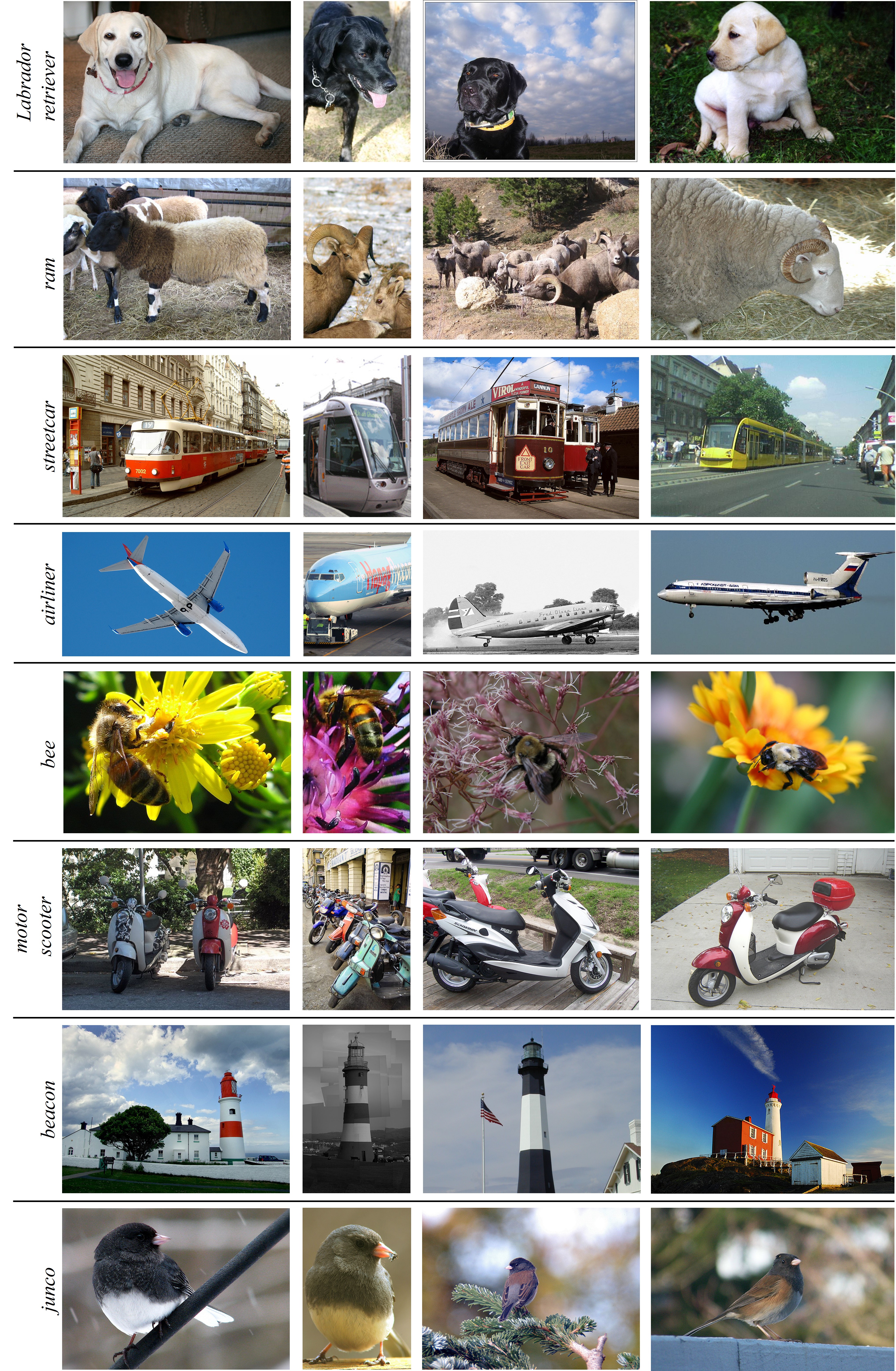
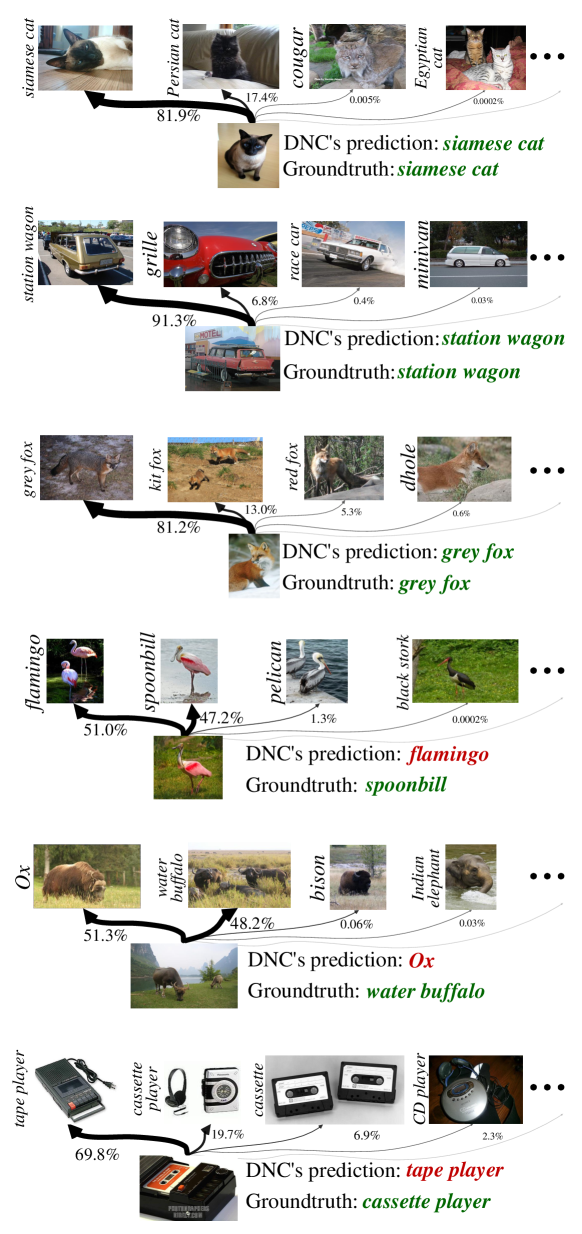
Appendix M Qualitative Results on Semantic Segmentation
Fig. 7 and Fig. 8 illustrate a few representative visual examples of semantic segmentation results on ADE20K [37] and Cityscapes [26], respectively. In comparison with the parametric counterpart, our approach produces more precise segments in different challenging scenes (for example, where objects with drastic photometric or geometric appearances). For instance, UperNet [36]-Swin-B [3] confuses on neighbouring objects with similar colors (, desk and chair) and leaves a large false-negative regions (see the first image of Fig. 7); it also has difficulties in segmenting small scale objects (, motorbike semantic parsing). Among these examples, DNC consistently demonstrates supreme performance. Essentially, we argue that the proposed DNC has a stronger ability to supervises the pixel embedding space via anchoring sub-centroids directly, leading to a better predictions on segmenting such hard cases.
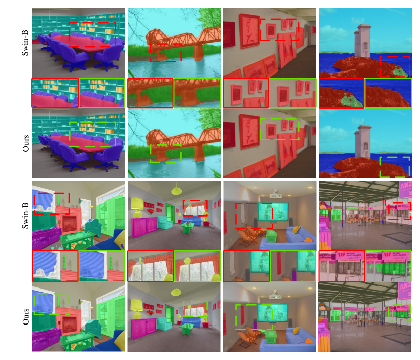
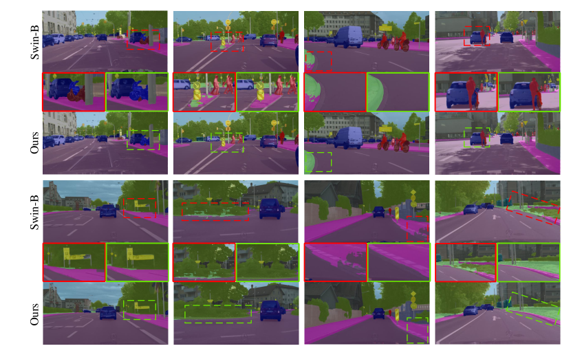
Appendix N Additional Literature Review
This section gives additional review of representative literature on metric-/distance-learning and clustering-based unsupervised representation learning.
Metric Learning. The goal of metric learning (also a.k.a distance learning) is to learn a distance metric/embedding which brings together similar samples and pushes away dissimilar ones. Metric learning has a long history, dating back to some early work for more than few decades ago [113, 114]. In particular, diverse metric learning objective functions, such as contrastive loss [115, 87, 93], triplet loss [116], quadruplet loss [117], and -pair loss [88], were proposed to measure similarity in the feature space for representation learning, and showed significant benefit in a wide range of applications, such as image retrieval [118], face recognition [116, 119, 120, 121, 122], and person re-identification [123], to name a few representative ones. Recently, metric learning gained astonishing success in learning transferable deep representations from massive unlabeled data [89]. A family of instance-based approaches used the contrastive loss [124, 125] to explicitly compare pairs of image representations [125, 126, 127, 128, 129]. Another group of methods adopted a clustering-based strategy; they learn unsupervised representations by discriminating between groups of images without expensive pairwise comparison between image instances [94, 95, 96, 97, 98, 99, 24, 100, 101]. More recently, there are some efforts that revisit the idea of metric learning in supervised learning setting [93, 91, 92, 112].
As distance-/similarity-based classifiers rely on the similarity between samples and class representatives for classification, the fields of metric learning and distance-based classification are naturally related and the selection of a proper distance measure impacts the success of distance-based classifiers [130]. Historically, metric learning and class center discovery are two critical research topics in the field of distance-based classification. As a nonparametric, distance-based classifier, DNC can be viewed as a learnable metric function, which is trained to compare data samples under the guidance of the corresponding semantic labels. Although current distance learning based algorithms also optimize the feature space by comparing data samples, they need parametric softmax for classification. Their trained models are still black-box parametric classifiers without any interpretability. In sharp contrast, DNC directly assigns an observation to the class of the closet centroids, without using parametric softmax. Moreover, its distance-based classification decision-making mode allows DNC to effortless adopt existing metric learning techniques (and the way of its current training can be already viewed as performing metric learning).
Clustering-based Self-supervised Representation Learning. There is a recent trend to bind self-supervised representation learning with clustering. Basically, clustering-based self-supervised representation learning is more efficient for large-scale training data and more tolerant of the similarity (semantic structure) among data samples, compared with the instance-level counterpart. More specifically, early approaches [94, 96, 131, 132, 97, 24, 100] learn representations of image samples and cluster assignments in an alternative manner, i.e., group features into clusters to derive pseudo supervisory signal and subsequently employ it for supervising representation learning. In very recent, numerous efforts have been devoted to simultaneous clustering and representation learning based on, e.g., data reconstruction [95, 133], mutual information maximization [131, 134, 135], or contrastive instance discrimination [136, 137, 138, 98, 99, 101].
Our work is also related to these clustering based unsupervised representation learning methods, especially the ones [24, 98] resorting to the fast Sinkhorn-Knopp algorithm [23] for robust clustering. They aim to learn transferable representation from massive unlabeled data. Although also involving a similar clustering procedure for automatic sub-pattern mining, DNC targets at building a strong similarity-based classification network in the standard supervised learning setting. In DNC, the automatically discovered class sub-centroids are informative class representatives, which explicitly capture latent data structure of each class, and serve as classification evidence with clear physical meaning. The whole training procedure is a hybrid of class-wise online clustering (for unsupervised sub-class discovery) and sub-centroid based classification (for supervised representation learning). This well addresses the nature of Nearest Centroids and brings novel insights into the visual recognition task itself.
Appendix O Limitation and Future Work
Limitation. One limitation of our approach is that the Sinkhorn-Knopp algorithm runs in time which would reduce the training efficiency. Though in practice, we find 3 sinkhorn loops per training iteration is sufficient enough for model representation, bringing a minor computational overhead (, 5% training delay on ImageNet). This also indicates possible directions for our future research.
Social Impact. This work introduces DNC possessing the nature of nested simplicity, intuitive decision-making mechanism and even ad-hoc explainability. On positive side, the approach advances model accuracy and is valuable in safety-sensitive applications by showing the advanced robustness on sub-categories discovery, , quality analytics, autonomous driving [139, 140, 141], etc.. For potential negative social impact, our DNC struggles in handling out-of-distribution data, which is a common limitation of all the discriminative classifiers. Hence its utility in open-world scenarios should be further examined.
Future Work. Despite DNC’s systemic simplicity and efficacy, it also comes with new challenges and unveils some intriguing questions. For example, incorporating more powerful, time-efficient online clustering algorithms into DNC might improve training speed and test accuracy. Also, the number of class centroids currently is set to a fixed value for all classes, which may not be optimal given that intra-class variability varies across classes. Our experiments in §J and Table 23 also suggest that simply varying with the number of training samples of the class can boost performance. Thus adopting the clustering algorithms that do not require a predefined and fixed number of clusters [142] may allow DNC to automatically determine for different classes, which eventually benefit performance. In addition, instead of only considering first-order statistics, DNC could be enhanced by second-order statistics, which contain more useful information, but must contend with the computational overhead they impose. Another essential future direction deserving of further investigation is the in-depth analysis of the intrinsic properties of DNC, such as its robustness against perturbation, adversarial attack [143, 144], and out-of-distribution data, with the comparison of the softmax based counterpart. This endeavor would help us to better understand the nature of parametric and nonparametric classifiers and reveals directions for further improvement. Furthermore, we will explore the possibility of unifying close-set and open-world visual recognition within our framework. Finally, considering the similarity-/distance-based nature of DNC, the incorporation of metric learning based training objectives is also another promising direction for further boosting the performance. Given the vast number of technique breakthroughs in recent years, we expect a flurry of innovation towards these promising directions. Overall, we believe the results presented in this paper warrant further exploration.