Optimal vaccinations: Cordons sanitaires, reducible population and optimal rays

Abstract.

We consider the bi-objective problem of allocating doses of a (perfect) vaccine to an infinite-dimensional metapopulation in order to minimize simultaneously the vaccination cost and the effective reproduction number $R_{e}$, which is defined as the spectral radius of the effective next-generation operator.

In this general framework, we prove that a cordon sanitaire, that is, a strategy that effectively disconnects the non-vaccinated population, might not be optimal, but it is still better than the “worst” vaccination strategies. Inspired by graph theory, we also compute the minimal cost which ensures that no infection occurs using independent sets. Using Frobenius decomposition of the whole population into irreducible subpopulations, we give some explicit formulae for optimal (“best” and “worst”) vaccinations strategies. Eventually, we provide some sufficient conditions for a scaling of an optimal strategy to still be optimal.

1. Introduction

1.1. Vaccination in metapopulation models

In metapopulation epidemiological models, the population is composed of $N$ subpopulations labelled $1,\ldots,N$, of respective sizes $\mu_{1},\ldots,\mu_{N}$. Following [hill-longini-2003], much of the behaviour of the epidemic may be derived from the so called next-generation matrix $K=(K_{ij})_{1\leq i,j\leq N}$, where $K_{ij}$ corresponds to an expected number of secondary infections for people in subpopulation $i$ resulting from a single randomly selected non-vaccinated infectious person in subpopulation $j$.

A vaccination strategy is represented by a vector $\eta\in\Delta=[0,1]^{N}$, where $\eta_{i}$ is the fraction of non-vaccinated individuals in the $i$^th subpopulation. In particular, $\eta_{i}$ is equal to $0$ when the $i$^th subpopulation is fully vaccinated, and $1$ when it is not vaccinated at all. The strategy $\mathbb{1}\in\Delta$, with all its entries equal to 1, therefore corresponds to an entirely non-vaccinated population. The spectral radius (i.e., the largest modulus of the eigenvalues) of $K\cdot\mathrm{Diag}(\eta)$, denoted $R_{e}(\eta)$, is referred to as the effective reproduction number, and may then be interpreted as the expected number of cases directly generated by one typical case where all non-vaccinated individuals are susceptible to the infection. In particular, we denote by $R_{0}=R_{e}(\mathbb{1})$ the so-called basic reproduction number associated to the metapopulation epidemiological model. We refer to Section 2 for the computation of the reproduction number for a wide-class of compartmental metapopulation models appearing in the literature.

With this interpretation of the reproduction number in mind, it is then natural to minimize it on the space $\Delta$ under a constraint on the cost $C$. A natural choice for the cost function is given by the uniform cost $C_{\mathrm{uni}}(\eta)=\sum_{i}(1-\eta_{i})\mu_{i}$, which corresponds to the fraction of vaccinated individuals in the population. This constrained optimization problem appears in most of the literature for designing efficient vaccination strategies for multiple epidemic situation (SIR/SEIR) [EpidemicsInHeCairns1989, hill-longini-2003, TheMostEfficiDuijze2016, CriticalImmuneMatraj2012, poghotanyan_constrained_2018, OptimalInfluenEnayat2020, IdentifyingOptZhao2019]. Note that in some of these references, the effective reproduction number is defined as the spectral radius of the matrix $\mathrm{Diag}(\eta)\cdot K$. Since the eigenvalues of $\mathrm{Diag}(\eta)\cdot K$ are exactly the eigenvalues of the matrix $K\cdot\mathrm{Diag}(\eta)$, this actually defines the same function $R_{e}$.

The goal of this paper is to prove a number of properties of the optimal vaccination strategies associated to a bi-objective optimization problem with cost function $C$ and loss function $R_{e}$, that shed a light on how to vaccinate in the best possible way. In previous works [delmas_infinite-dimensional_2020, ddz-theo], we introduced a general kernel framework in which the matrix formulation appears as a special finite-dimensional case. We state our results in this general framework, but for ease of the presentation, we shall stick to the matrix formulation in this introduction. We also refer the interested reader to [ddz-Re] for a detailed study of $R_{e}$ and its convexity property, and to [ddz-reg] for various examples of kernels and optimal vaccination strategies.

In our previous work [ddz-theo], we assumed only minimal hypothesis on the so-called loss function whose aims to measure the vulnerability of the population. Here, we choose to take the effective reproduction number as the loss. We also consider strictly decreasing cost functions (because vaccinating more people costs more; see Section 3.4). These more restrictive assumptions allow us to simplify some of the statements made in [ddz-theo] and to give additional specific results.

In bi-objective optimization, one can identify Pareto (resp. anti-Pareto) optimal vaccinations strategies, informally “best” (resp. “worst”) vaccination strategies, in the sense that every strategy that does strictly better for one objective must do strictly worse for the other (resp. every strategy that does strictly worse for one objective must do strictly better for the other). We refer to [ddz-theo, Section 5] for details. We also consider the Pareto frontier $\mathcal{F}$ (resp. anti-Pareto frontier $\mathcal{F}^{\mathrm{Anti}}$) as the outcomes $(C(\eta),R_{e}(\eta))$ of the Pareto (resp. anti-Pareto) optimal strategies $\eta$; see Section 3.4. In Figure 1(a), we have plotted in red the Pareto frontier and in a dashed red line the anti-Pareto frontier when the next-generation matrix is the adjacency matrix of the non-oriented cycle graph with $N=12$ nodes from Figure 2(a) and Example 1.1; see also Example 2.1.

(a) Thick red line: Pareto frontier; Dashed line: anti-Pareto frontier; x marker: outcomes of various strategies; light blue: all possible outcomes $(C(\eta),R_{e}(\eta))$ for $\eta\in\Delta$.

(b) Profile of various strategies.

Figure 1. Performance of the disconnecting vaccination strategy “one in $4$” for the non-oriented cycle graph with 12 nodes and uniform cost $3$.

1.2. A cordon sanitaire is not the worst vaccination strategy

Recall that a matrix $K$ is reducible if there exists a permutation $\sigma$ such that $(K_{\sigma(i)\sigma(j)})_{i,j}$ is block upper triangular, and irreducible otherwise. A cordon sanitaire is a vaccination strategy $\eta$ such that the effective next-generation matrix $K\cdot\mathrm{Diag}(\eta)$ is reducible. Informally, such a strategy splits the effective population in at least two groups, one of which does not infect the other.

Disconnecting the population by creating a cordon sanitaire is not always the “best” choice, that is, it may not be Pareto optimal. However, we prove in Proposition 5.3 that a cordon sanitaire can never be anti-Pareto optimal; this result still holds in the general kernel framework, provided that the definition of a cordon sanitaire is generalized in an appropriate way.

Example 1.1 (Non-oriented cycle graph).

Suppose that the matrix $K$ is given by the adjacency matrix of the non-oriented cycle graph with $N=12$ nodes and $\mu$ is the counting measure; see Figure 2(a) for the graph drawing and Figure 2(b) for the grayscale representation of its corresponding kernel. For a cost $C_{\mathrm{uni}}=3$, there is a cordon sanitaire $\eta$ that consists in vaccinating one subpopulation in four; see Figure 2(c) and Figure 2(d). The effective reproduction number is then equal to $\sqrt{2}$. This strategies performs better than the anti-Pareto optimal strategy but it is not Pareto optimal as we can see in Figure 1. This example is discussed in detail in [ddz-reg, Section 2.4].

(a) The non-oriented cycle graph.

(b) Grayscale representation of the corresponding kernel.

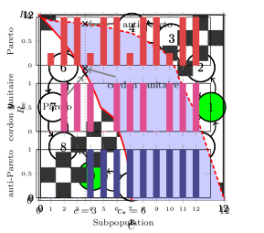
(c) Cordon sanitaire corresponding to the “one in $4$” vaccination strategy. In green the vaccinated subpopulations.

(d) Grayscale representation of the corresponding effective kernel.

Figure 2. Example of disconnecting vaccination strategy on the non-oriented cycle graph with $N=12$ nodes. The kernels are defined on the square $[0,12]\times[0,12]$ equipped with the Lebesgue measure.

1.3. Minimal cost required to completely stop the transmission of the disease

Suppose that the next-generation matrix is symmetric. Then, a vaccination strategy $\eta$ such that $R_{e}(\eta)=0$ completely stops the transmission of the infection. Section 4.2 is devoted to the computation of the minimal cost for achieving this goal. We give in Proposition 4.4 an explicit expression of this quantity in the kernel model. When $K$ is the adjacency matrix of a graph of size $N$, $\mu$ is the counting measure over the set of nodes and the cost is uniform, this expression is equal to the size of maximal independent sets. We observe this property in Figure 1(a) as the size of the maximal independent set of the non-oriented cycle graph from Example 1.1 is equal to $\left\lfloor\,N/2\,\right\rfloor$.

1.4. Reducible case

When the matrix $K$ happens to be reducible, up to a relabeling, we may assume that it is block upper triangular. Denoting by $m$ the number of blocks and $I_{1},\ldots,I_{m}$ the sets of indices describing the blocks, this means that for all $\ell>k$ and $(i,j)\in I_{\ell}\times I_{k}$, we have $K_{ij}=0$. In the epidemiological interpretation, this means that the populations with indices in $I_{k}$ never infect the ones with indices in $I_{\ell}$. One may then hope that the study of $R_{e}$ can be effectively reduced to the study of the effective radius of the square sub-matrices $(K_{ij})_{i,j\in I_{k}}$ describing the infections within block $I_{k}$. This is indeed the case, and we give in Section 5.4 a complete picture of the Pareto and anti-Pareto frontiers of $R_{e}$, in terms of the effective reproduction numbers restricted to each irreducible component of the infection kernel or matrix. In particular, this allows a better understanding of why the anti-Pareto frontier may be discontinuous, while the Pareto frontier is always continuous. For the reduction to each irreducible component to be effective for the Pareto frontier, one has to assume that the cost function is extensive: the cost of vaccinating disjoint subsets of the population is additive. Once more, special care has to be taken with the definitions when handling the infinite dimensional kernel case.

1.5. Optimal ray

It is observed by Poghotanyan, Feng, Glasser and Hill in [poghotanyan_constrained_2018, Theorem 4.3], that in the finite dimensional case, under an assumption that ensures the convexity of the function $R_{e}$, and for a uniform cost, if there exists a Pareto optimal strategy $\eta$ with all its entries strictly less than 1, then all the strategies $\lambda\eta$, with $\lambda\geq 0$ such that $\lambda\eta\in\Delta$, are Pareto optimal. We give a short proof on the existence of such optimal rays in Section 4.1 in a general kernel framework, when the cost function $C$ is affine and $R_{e}$ is convex on $\Delta$.

1.6. Organization of the paper

We present in Section 2 different models for which the effective reproduction number associated to an epidemic model with vaccination can be seen as the spectral radius of a compact operator. In Section 3, we present the mathematical framework for the study of the effective reproduction function and the associated bi-objective problems with a general cost function as well as the Pareto and anti-Pareto frontiers. Section 4 is devoted to the description of optimal vaccination strategies which eradicate the epidemic, and the possible existence of optimal rays in the Pareto frontier. Using a Frobenius decomposition of the next generation kernel in Section 5.1, we first complete the description of the anti-Pareto frontier in the irreducible and monatomic cases in Section 5.2. We study in Section 5.3 the optimality of cordons sanitaires vaccination strategies and show in Section 5.4 how the optimization problem may be effectively reduced to the study on subpopulations when the next generation kernel is reducible.

2. Generality of the effective next-generation operator

In [delmas_infinite-dimensional_2020, ddz-theo], we developed a framework that we call the kernel model where the population is represented as an abstract measure space $(\Omega,\mathscr{F},\mu)$, with $\mu$ non-zero $\sigma$-finite measure. Individuals are characterized by a trait $x\in\Omega$. The size of the subpopulation with trait $x$ is given by $\mu(\mathrm{d}x)$. The underlying structure described by this trait can be very diverse. Typical examples include spatial position, social contacts, susceptibility, infectiousness, characteristics of the immunological response, etc. The analogue of the next-generation matrix $K$ is the kernel operator defined formally by:

$$T_{\mathrm{k}}(g)(x)=\int_{\Omega}\mathrm{k}(x,y)\,g(y)\,\mathrm{d}\mu(y),$$

where the non-negative kernel $\mathrm{k}$ is defined on $\Omega\times\Omega$ and $\mathrm{k}(x,y)$ still represents a strength of infection from $y$ to $x$. Vaccination strategies $\eta\,\colon\,\Omega\to[0,1]$ encode the density of non-vaccinated individuals with respect to the measure $\mu$. So, the strategy $\eta=\mathbb{1}$, the constant function equal to 1, corresponds to no vaccination in the population, whereas the strategy $\eta=\mathbb{0}$, the constant function equal to 0, corresponds to all the population being vaccinated. The measure $\eta(y)\,\mu(\mathrm{d}y)$ may then be understood as an effective population, giving rise to an effective next-generation operator:

$$T_{\mathrm{k}\eta}(g)(x)=\int_{\Omega}\mathrm{k}(x,y)\,g(y)\,\eta(y)\,\mu(\mathrm{d}y).$$

The effective reproduction number is then defined by $R_{e}(\eta)=\rho(T_{\mathrm{k}\eta})$, where $\rho$ stands for the spectral radius of the operator and $\mathrm{k}\eta$ for the kernel $(\mathrm{k}\eta)(x,y)=\mathrm{k}(x,y)\eta(y)$.

The results mentioned in the introduction will be given in this general framework, which is flexible enough to describe a wide range of epidemic models from the literature including the metapopulation models. In the following of the Section, we give a few examples to support this claim. In each of them, the spectral radius of a given explicit kernel operator appears as a threshold parameter, and the epidemic either expands or dies out depending on the value of this parameter. Classical notations are used: $S$ denotes the proportion of susceptible individuals, $E$ the proportion of those who have been exposed to the disease, $I$ the proportion of infected individuals, $R$ the proportion of removed individuals in the population. Thus $I(t,x)$ denotes the proportion of the population with trait $x\in\Omega$ which is infected at time $t\geq 0$. In the following examples, the measure $\mu$ is assumed to be a probability measure.

Example 2.1 (Metapopulation models).

Recall that in metapopulation models, the population is divided into $N\geq 2$ different subpopulations of respective proportional size $\mu_{1},\ldots,\mu_{N}$, and the reproduction number is given by $R_{e}(\eta)=\rho(K\cdot\mathrm{Diag}(\eta))$, where $K$ is the next generation matrix and $\eta$ belongs to $[0,1]^{N}$ and gives the proportion of non-vaccinated individuals in each subpopulation. To express the function $R_{e}$ as the effective reproduction number of a kernel model, consider the discrete state space $\Omega_{\mathrm{d}}=\{1,\ldots,N\}$ equipped with the probability measure $\mu_{\mathrm{d}}$ defined by $\mu_{\mathrm{d}}(\{i\})=\mu_{i}$, and let $\mathrm{k}_{\mathrm{d}}$ denote the discrete kernel on $\Omega_{\mathrm{d}}$ defined by:

(1) $$\mathrm{k}_{\mathrm{d}}(i,j)=K_{ij}/\mu_{j}.$$

For all $\eta\in\Delta=[0,1]^{N}$, the matrix $K\cdot\mathrm{Diag}(\eta)$ is the matrix representation of the endomorphism $T_{\mathrm{k}_{\mathrm{d}}\eta}$ in the canonical basis of $\mathbb{R}^{N}$. In particular, we have: $R_{e}(\eta)=\rho(T_{\mathrm{k}\eta})=\rho(K\cdot\mathrm{Diag}(\eta))$.

In Figure 2(b), we have plotted a kernel on $[0,1]$ endowed with the usual Borel $\sigma$-algebra and the Lebesgue measure. This kernel is equivalent to $\mathrm{k}_{\mathrm{d}}$ when $K$ is the adjacency matrix of the non-oriented cycle graph and all subpopulations have the same size.

Example 2.2 (An SIR model with nonlinear incidence rate and vital dynamics).

In [thieme_global_2011], Thieme proposed an SIR model in an infinite-dimensional population structure with a nonlinear incidence rate. The structure space is given by $\Omega$ a compact subset of $\mathbb{R}^{N}$ with nonempty interior equipped with the Lebesgue measure denoted by $\mu$. We restrict slightly his assumptions so that the incidence rate is a linear function of the number of susceptible. Besides, we write explicitly the equation giving the evolution of the recovered compartment. It does not play a role in the long-time behavior analysis of the equations made by Thieme but it helps to understand the model when taking into account the vaccination. The dynamic of the epidemic then writes:

(2) $$\text{For $t\geq 0,x\in\Omega$,}\,\,\left\{\begin{array}[]{ll}\partial_{t}S(t,x)=\Lambda(x)-\nu_{S}(x)S(t,x)-S(t,x)\,\int_{\Omega}f(I(t,y),x,y)\,\mu(\mathrm{d}y),\\ \\ \partial_{t}I(t,x)=S(t,x)\,\int_{\Omega}f(I(t,y),x,y)\,\mu(\mathrm{d}y)-(\gamma(x)+\nu_{I}(x))I(t,x),\\ \\ \partial_{t}R(t,x)=\gamma(x)I(t,x)-\nu_{R}(x)R(t,x),\end{array}\right.$$

where, at location $x\in\Omega$:

• $\Lambda(x)$ is the rate at which fresh susceptible individuals are recruited,

• $\nu_{S}(x)$, $\nu_{I}(x)$, $\nu_{R}(x)$ are the per capita death rate of the susceptible, infected and recovered individuals respectively,

• $\gamma(x)$ is the per capita recovery rate of infected individuals,

• the integral term describes the incidence at time $t$, i.e., the rate of new infections.

The threshold parameter identified in [thieme_global_2011], that plays the role of the reproduction number, is given by the spectral radius of the operator $T_{\mathrm{k}}$ with the kernel $\mathrm{k}$ given by:

$$\mathrm{k}(x,y)=\frac{\Lambda(x)}{\nu_{S}(x)(\gamma(x)+\nu_{I}(x))}\partial_{I}f(0,x,y),\quad x,y\in\Omega,$$

where $\partial_{I}f(0,x,y)$, the derivative of $f$ with respect to its first variable $I$, is supposed to be non-negative.

Suppose that individuals at location $x$ are vaccinated with probability $1-\eta(x)$ at birth. In the corresponding model, the rate at which susceptible individuals with trait $x$ are recruited becomes equal to $\eta(x)\Lambda(x)$ while recovered/immunized individuals are recruited at rate $(1-\eta(x))\Lambda(x)$ at location $x$ so that the dynamic of the recovered compartment is given by:

$$\partial_{t}R(t,x)=(1-\eta(x))\Lambda(x)+\gamma(x)I(t,x)-\nu_{R}(x)R(t,x),\qquad x\in\Omega,\,t\geq 0.$$

The threshold parameter $R_{e}(\eta)$ is then given by the spectral radius of the integral operator $T_{\eta\mathrm{k}}$ with kernel $\eta\mathrm{k}$ given by $(\eta\mathrm{k})(x,y)=\eta(x)\mathrm{k}(x,y)$. According to Equation (7), we have $\rho(T_{\eta\mathrm{k}})=\rho(T_{\mathrm{k}\eta})$, and our framework can be used for this model.

Under regularity assumptions on the parameters of the model, Thieme proved that if $R_{e}(\eta)$ is greater than $1$, then there exists an endemic equilibrium that attracts all the solutions while if $R_{e}(\eta)$ is smaller than $1$, then $I(t,x)$ converges to $0$ for all $x\in\Omega$ as $t$ goes to infinity.

Example 2.3 (An SEIR model without vital dynamics).

In [FinalSizeAndAlmeid2021], Almeida, Bliman, Nadin and Perthame studied an heterogeneous SEIR model where the population is again structured with a bounded subset $\Omega\subset\mathbb{R}^{N}$ with nonempty interior equipped with the Lebesgue measure denoted by $\mu$. This time however there is no birth nor death of the individuals. The dynamic of the susceptible, exposed, infected and recovered individuals writes:

(3) $$\text{For $t\geq 0$, $x\in\Omega$,}\qquad\left\{\begin{array}[]{ll}\partial_{t}S(t,x)=-S(t,x)\,\int_{\Omega}k(x,y)I(t,y)\,\mu(\mathrm{d}y),\\ \\ \partial_{t}E(t,x)=S(t,x)\,\int_{\Omega}k(x,y)I(t,y)\,\mu(\mathrm{d}y)-\alpha(x)E(t,x),\\ \\ \partial_{t}I(t,x)=\alpha(x)E(t,x)-\gamma(x)I(t,x),\\ \\ \partial_{t}R(t,x)=\gamma(x)I(t,x).\end{array}\right.$$

Here, the average incubation rate is denoted by $\alpha(x)$ and the average recovery rate by $\gamma(x)$; both quantities may depend upon the trait $x$. The function $k$ is the transmission kernel of the disease. In this model, the basic reproduction number is given by the spectral radius of the integral operator $T_{\mathrm{k}}$ with kernel $\mathrm{k}=k/\gamma$ given by:

(4) $$\mathrm{k}(x,y)=k(x,y)/\gamma(y).$$

Note that the basic reproduction number does not depend on the average incubation rate $\alpha$ as in the one-dimensional SEIR model with constant population size; see [driessche, Section 2.2] with death rate $d=0$.

Suppose that, prior to the beginning of the epidemic, the decision maker immunizes a density $1-\eta$ of individuals. According to [FinalSizeAndAlmeid2021, Section 3.2], the effective reproduction number is given by $\rho(T_{\eta\mathrm{k}})$ which is also equal to $\rho(T_{\mathrm{k}\eta})$. Hence, our model is indeed suitable for designing optimal vaccination strategies in this context.

Example 2.4 (An SIS model without vital dynamic).

In [delmas_infinite-dimensional_2020], generalizing the discrete model of Lajmanovich and Yorke [lajmanovich1976deterministic], we introduced the following heterogeneous SIS model where the population is structured with an abstract probability space $(\Omega,\mathscr{F},\mu)$:

(5) $$\text{For $t\geq 0$, $x\in\Omega$,}\qquad\left\{\begin{array}[]{ll}\partial_{t}S(t,x)=-S(t,x)\,\int_{\Omega}k(x,y)I(t,y)\,\mu(\mathrm{d}y)+\gamma(x)I(t,x),\\ \\ \partial_{t}I(t,x)=S(t,x)\,\int_{\Omega}k(x,y)I(t,y)\,\mu(\mathrm{d}y)-\gamma(x)I(t,x).\end{array}\right.$$

The function $\gamma$ is the per-capita recovery rate and $k$ is the transmission kernel. For this model, $R_{e}(\eta)=\rho(T_{\mathrm{k}\eta})$ where $\mathrm{k}=k/\gamma$ is defined by $\mathrm{k}(x,y)=k(x,y)/\gamma(y)$.

Suppose that, prior to the beginning of the epidemic, a density $1-\eta$ of individuals is vaccinated with a perfect vaccine. In the same way as for the SEIR model, we proved, as $t$ goes to infinity, that if $R_{e}(\eta)$ is smaller than or equal to $1$, then $I(t,\cdot)$ converges to $0$, and, under a connectivity assumption on the kernel $k$, that if $R_{e}(\eta)$ is greater than $1$, then $I(t,\cdot)$ converges to the (unique) positive endemic equilibrium. This highlights the importance of $R_{e}$ in the design of vaccination strategies.

3. Setting, notations and previous results

3.1. Spaces, operators, spectra

All metric spaces $(S,d)$ are endowed with their Borel $\sigma$-field denoted by $\mathscr{B}(S)$. Let $(\Omega,\mathscr{F},\mu)$ be a measured space, with $\mu$ a $\sigma$-finite positive and non-zero measure. For $f$ and $g$ real-valued functions defined on $\Omega$, we write $\langle f,g\rangle$ or $\int_{\Omega}fg\,\mathrm{d}\mu$ for $\int_{\Omega}f(x)g(x)\,\mu(\mathrm{d}x)$ whenever the latter is meaningful. For $p\in[1,+\infty]$, we denote by $L^{p}=L^{p}(\mu)=L^{p}(\Omega,\mu)$ the space of real-valued measurable functions $g$ defined on $\Omega$ such that $\left\lVert\,g\,\right\rVert_{p}=\left(\int|g|^{p}\,\mathrm{d}\mu\right)^{1/p}$ (with the convention that $\left\lVert\,g\,\right\rVert_{\infty}$ is the $\mu$-essential supremum of $|g|$) is finite, where functions which agree $\mu$-a.e. are identified. We denote by $L^{p}_{+}$ the subset of $L^{p}$ of non-negative functions. We define $\Delta$ as the subset of $L^{\infty}$ of $[0,1]$-valued measurable functions defined on $\Omega$. We denote by $\mathbb{1}$ (resp. $\mathbb{0}$) the constant function on $\Omega$ equal to $1$ (resp. $0$); both functions belong to $\Delta$.

Let $(E,\left\lVert\,\cdot\,\right\rVert)$ be a complex Banach space. We denote by $\left\lVert\,\cdot\,\right\rVert_{E}$ the operator norm on $\mathcal{L}(E)$ the Banach algebra of linear bounded operators. The spectrum $\operatorname{Spec}(T)$ of $T\in\mathcal{L}(E)$ is the set of $\lambda\in\mathbb{C}$ such that $T-\lambda\mathrm{Id}$ does not have a bounded inverse, where $\mathrm{Id}$ is the identity operator on $E$. Recall that $\operatorname{Spec}(T)$ is a compact subset of $\mathbb{C}$, and that the spectral radius of $T$ is given by:

(6) $$\rho(T)=\max\{|\lambda|\,\colon\,\lambda\in\operatorname{Spec}(T)\}=\lim_{n\rightarrow\infty}\left\lVert\,T^{n}\,\right\rVert_{E}^{1/n}.$$

The element $\lambda\in\operatorname{Spec}(T)$ is an eigenvalue if there exists $x\in E$ such that $Tx=\lambda x$ and $x\neq 0$.

Recall that the spectrum of a compact operator is finite or countable and has at most one accumulation point, which is $0$. Furthermore, $0$ belongs to the spectrum of compact operators in infinite dimension. If $A\in\mathcal{L}(E)$ is compact and $B\in\mathcal{L}(E)$, then both $AB$ and $BA$ are compact and:

(7) $$\rho(AB)=\rho(BA).$$

We refer to [schaefer_banach_1974] for an introduction to Banach lattices and positive operators. We shall only consider the real Banach lattices $L^{p}=L^{p}(\Omega,\mu)$ for $p\in[1,+\infty]$ on a measured space $(\Omega,\mathscr{F},\mu)$ with a $\sigma$-finite non-zero measure, as well as their complex extension. (Recall that the norm of an operator on $L^{p}$ or its natural complex extension is the same according to [complex, Corollary 1.3]). A bounded operator $A$ is positive if $A(L^{p}_{+})\subset L^{p}_{+}$. If $A,B\in\mathcal{L}(L^{p})$ and $A-B$ are positive operators, then:

(8) $$\rho(A)\geq\rho(B).$$

If $E$ is also a real or complex function space, for $g\in E$, we denote by $M_{g}$ the multiplication operator (possibly unbounded) defined by $M_{g}(h)=gh$ for all $h\in E$. If furthermore $g$ is the indicator function of a set $A$, we simply write $M_{A}$ for $M_{\mathbb{1}_{A}}$.

3.2. Kernel operators

We define a kernel (resp. signed kernel) on $\Omega$ as a $\mathbb{R}_{+}$-valued (resp. $\mathbb{R}$-valued) measurable function defined on $(\Omega^{2},\mathscr{F}^{\otimes 2})$. For $f,g$ two non-negative measurable functions defined on $\Omega$ and $\mathrm{k}$ a kernel on $\Omega$, we denote by $f\mathrm{k}g$ the kernel defined by:

(9) $$f\mathrm{k}g:(x,y)\mapsto f(x)\,\mathrm{k}(x,y)g(y).$$

For $p\in(1,+\infty)$, we define the double norm of a signed kernel $\mathrm{k}$ on $L^{p}$ by:

(10) $$\left\lVert\,\mathrm{k}\,\right\rVert_{p,q}=\left(\int_{\Omega}\left(\int_{\Omega}\left\lvert\,\mathrm{k}(x,y)\,\right\rvert^{q}\,\mu(\mathrm{d}y)\right)^{p/q}\mu(\mathrm{d}x)\right)^{1/p}\quad\text{with~{}$q$ given by}\quad\frac{1}{p}+\frac{1}{q}=1.$$

We say that $\mathrm{k}$ has a finite double norm, if there exists $p\in(1,+\infty)$ such that $\left\lVert\,\mathrm{k}\,\right\rVert_{p,q}<+\infty$. To such a kernel $\mathrm{k}$, we then associate the positive integral operator $T_{\mathrm{k}}$ on $L^{p}$ defined by:

(11) $$T_{\mathrm{k}}(g)(x)=\int_{\Omega}\mathrm{k}(x,y)\,g(y)\,\mu(\mathrm{d}y)\quad\text{for }g\in L^{p}\text{ and }x\in\Omega.$$

According to [grobler, p. 293], the operator $T_{\mathrm{k}}$ is compact. It is well known and easy to check that:

(12) $$\left\lVert\,T_{\mathrm{k}}\,\right\rVert_{L^{p}}\leq\left\lVert\,\mathrm{k}\,\right\rVert_{p,q}.$$

We define the reproduction number associated to the operator $T_{\mathrm{k}}$ as:

(13) $$R_{0}[\mathrm{k}]=\rho(T_{\mathrm{k}}).$$

3.3. The effective reproduction number $R_{e}$

A vaccination strategy $\eta$ of a vaccine with perfect efficiency is an element of $\Delta$, where $\eta(x)$ represents the proportion of non-vaccinated individuals with feature $x$, so that the constant functions $\eta=\mathbb{1}$ and $\eta=\mathbb{0}$ correspond respectively to no vaccination and complete vaccination. Notice that $\eta\,\mathrm{d}\mu$ corresponds in a sense to the effective population. Let $\mathrm{k}$ be a kernel on $\Omega$ with finite double norm on $L^{p}$. For $\eta\in\Delta$, the operator $M_{\eta}$ is bounded on $L^{p}$, whence the operator $T_{\mathrm{k}\eta}=T_{\mathrm{k}}M_{\eta}$ is compact. We define the effective reproduction number function $R_{e}[\mathrm{k}]$ from $\Delta$ to $\mathbb{R}_{+}$ by:

(14) $$R_{e}[\mathrm{k}](\eta)=\rho(T_{\mathrm{k}\eta}),$$

and the corresponding reproduction number is then given by $R_{0}[\mathrm{k}]=R_{e}[\mathrm{k}](\mathbb{1})$. When there is no risk of confusion on the kernel $\mathrm{k}$, we simply write $R_{e}$ and $R_{0}$ for the function $R_{e}[\mathrm{k}]$ and the number $R_{0}[\mathrm{k}]$.

We can see $\Delta$ as a subset of $L^{\infty}$, and consider the corresponding weak-* topology: a sequence $(g_{n},n\in\mathbb{N})$ of elements of $\Delta$ converges weakly-* to $g$ if for all $h\in L^{1}$ we have:

(15) $$\lim\limits_{n\to\infty}\int_{\Omega}hg_{n}\,\mathrm{d}\mu=\int_{\Omega}hg\,\mathrm{d}\mu.$$

The set $\Delta$ endowed with the weak-* topology is compact and sequentially compact [ddz-theo, Lemma 3.1]. We also recall the properties of the effective reproduction number given in [ddz-theo, Proposition 4.1 and Theorem 4.2].

Proposition 3.1.

Let $\mathrm{k}$ be a finite double norm kernel on a measured space $(\Omega,\mathscr{F},\mu)$ where $\mu$ is a $\sigma$-finite non-zero measure Then, the function $R_{e}=R_{e}[\mathrm{k}]$ is a continuous function from $\Delta$ (endowed with the weak-* topology) to $\mathbb{R}_{+}$. Furthermore, the function $R_{e}=R_{e}[\mathrm{k}]$ satisfies the following properties:

1. $R_{e}(\eta_{1})=R_{e}(\eta_{2})$ if $\eta_{1}=\eta_{2},\,\mu\text{ a.s.}$, and $\eta_{1},\eta_{2}\in\Delta$,

2. $R_{e}(\mathbb{0})=0$ and $R_{e}(\mathbb{1})=R_{0}$,

3. $R_{e}(\eta_{1})\leq R_{e}(\eta_{2})$ for all $\eta_{1},\eta_{2}\in\Delta$ such that $\eta_{1}\leq\eta_{2}$,

4. $R_{e}(\lambda\eta)=\lambda R_{e}(\eta)$, for all $\eta\in\Delta$ and $\lambda\in[0,1]$.

3.4. Pareto and anti-Pareto frontiers

Let $\mathrm{k}$ be a kernel on $\Omega$ with a finite double norm. We consider the effective reproduction function $R_{e}=R_{e}[\mathrm{k}]$ defined on $\Delta$ as a loss function. We quantify the cost of the vaccination strategy $\eta\in\Delta$ by a function $C:\Delta\rightarrow\mathbb{R}^{+}$, and we assume that $C(\mathbb{1})=0$ (doing nothing costs nothing), $C$ is continuous for the weak-* topology on $\Delta$ defined in Section 3.3 and decreasing (doing more costs strictly more), that is, for any $\eta_{1},\eta_{2}\in\Delta$:

$$\eta_{1}\leq\eta_{2}\quad\text{and}\quad\mu(\eta_{1}<\eta_{2})>0\,\implies\,C(\eta_{1})>C(\eta_{2}).$$

For example, when the measure $\mu$ is finite, the uniform cost function:

(16) $$C_{\mathrm{uni}}(\eta)=\int_{\Omega}(1-\eta)\,\mathrm{d}\mu.$$

is continuous and decreasing on $\Delta$ (recall that $1-\eta$ represents the proportion of the population which has been vaccinated when using the strategy $\eta$.)

	“Best” vaccinations	“ Worst” vaccinations
Optimization problem	Pb (17): $\min_{\Delta}(C,R_{e})$	Pb (19): $\max_{\Delta}(C,R_{e})$
Opt. cost for a given loss defined on $[0,R_{0}]$, with $R_{0}:\,=\max_{\Delta}R_{e}=R_{e}(\mathbb{1})$.	$C_{\star}(\ell):\,=\min_{\,R_{e}\leq\ell}\,C$.	$C^{\star}(\ell):\,=\max_{\,R_{e}\geq\ell}\,C$.
	$C_{\star}$ is continuous.	2717
	$C_{\star}$ is decreasing.	$C^{\star}$ is decreasing.
	$C_{\star}(R_{0})=0$ and $c_{\star}\!:\,=C_{\star}(0)$.	$C^{\star}(0)=c_{\max}$ and $c^{\star}\!:\,=C^{\star}(R_{0})$.
Opt. loss for a given cost defined on $[0,c_{\max}]$, with $c_{\max}:\,=\max_{\Delta}C=C(\mathbb{0})$.	$R_{e\star}(c):\,=\min_{\,C\leq c}\,R_{e}$.	$R_{e}^{\star}(c):\,=\max_{\,C\geq c}\,R_{e}$.
	$R_{e\star}$ is continuous.	$R_{e}^{\star}$ is continuous.
	$R_{e\star}$ is decreasing on $[0,c_{\star}]$.	2717
	$R_{e\star}=0$ on $[c_{\star},c_{\max}]$.	$R_{e}^{\star}=R_{0}$ on $[0,c^{\star}]$.
	$R_{e\star}(0)=R_{0}$.	$R_{e}^{\star}(c_{\max})=0$.
Inverse formula	$R_{e\star}\circ C_{\star}=\mathrm{Id}\,$ on $[0,R_{0}]$.	$R_{e}^{\star}\circ C^{\star}=\mathrm{Id}\,$ on $[0,R_{0}]$.
	$C_{\star}\circ R_{e\star}=\mathrm{Id}\,$ on $[0,c_{\star}].$	2717
Optimal strategies	$\mathcal{P}:\,=\set{C=C_{\star}\circ R_{e}}\cap\set{R_{e}=R_{e\star}\circ C}$	$\mathcal{P}^{\mathrm{Anti}}:\,=\set{C=C^{\star}\circ R_{e}}\cap\set{R_{e}=R_{e}^{\star}\circ C}$
	$\phantom{\mathcal{P}:}=\set{C=C_{\star}\circ R_{e}}$	$\phantom{\mathcal{P}^{\mathrm{Anti}}:}=\set{C=C^{\star}\circ R_{e}}$
	$\phantom{\mathcal{P}:}=\set{R_{e}=R_{e\star}\circ C,\,C\leq c_{\star}}$.	$\phantom{\mathcal{P}^{\mathrm{Anti}}:}=\set{R_{e}=R_{e}^{\star}\circ C,\,C\geq c^{\star}}$.
	$\mathcal{P}$ is compact.	2717
Range of cost/loss	$\mathcal{A}:\,=[0,c_{\max}]\times[0,R_{0}]$
Possible outcomes	$\mathbf{F}:\,=(C,R_{e})(\Delta)\phantom{\mathcal{A}\,\colon\,R_{e\star}(c)\leq\ell\leq R_{e}^{\star}(c)}$
	$\phantom{\mathbf{F}:}=\set{(c,\ell)\in\mathcal{A}\,\colon\,R_{e\star}(c)\leq\ell\leq R_{e}^{\star}(c)}$
	$\phantom{\mathbf{F}:}=\set{(c,\ell)\in\mathcal{A}\,\colon\,C_{\star}(\ell)\leq c\leq C^{\star}(\ell)}.$
Optimal frontier	$\mathcal{F}:\,=(C,R_{e})(\mathcal{P})$	$\mathcal{F}^{\mathrm{Anti}}:\,=(C,R_{e})(\mathcal{P}^{\mathrm{Anti}})$
	$\phantom{\mathcal{F}:}=(C_{\star},\mathrm{Id})([0,R_{0}])$	$\phantom{\mathcal{F}^{\mathrm{Anti}}:}=(C^{\star},\mathrm{Id})([0,R_{0}])$.
	$\phantom{\mathcal{F}:}=(\mathrm{Id},R_{e\star})([0,c_{\star}])$.	2717
	$\mathcal{F}$ is connected and compact.	2717

The missing results, indicated by 2717, will be further completed under some additional conditions on the kernel $\mathrm{k}$ (see Proposition 5.1 for $\mathrm{k}$ positive and Corollary 5.2 for $\mathrm{k}$ monatomic).

Table 1. Summary of notation and results for the bi-objective problems.

In [ddz-theo], we formalized and study the problem of optimal allocation strategies for a perfect vaccine. This question may be viewed as a bi-objective minimization problem, where one tries to minimize simultaneously the cost of the vaccination and its loss given by the corresponding effective reproduction number:

(17) $$\min_{\Delta}(C,R_{e}).$$

Let us now briefly summarize the results from [ddz-theo]. For the reader’s convenience we also collect the main points in Table 1, and provide plots of typical Pareto and anti-Pareto frontiers in Figure 5. Note that Assumptions 4 and 5 in [ddz-theo] hold thanks to [ddz-theo, Lemma 5.13]. By definition, we have $R_{0}=\max_{\Delta}\,R_{e}$ and we set $c_{\max}=\max_{\Delta}C$ which is positive as $C$ is decreasing (and $\mu$ non-zero) and finite as $C$ is continuous and $\Delta$ compact. Related to the minimization problem (17), we shall consider $R_{e\star}$ the optimal loss function and $C_{\star}$ the optimal cost function defined by:

$$R_{e\star}(c) =\min\,\set{{R_{e}}(\eta)\,\colon\,\eta\in\Delta,\,C(\eta)\leq c}\quad\text{for $c\in[0,c_{\max}]$},$$

$$C_{\star}(\ell) =\min\,\set{C(\eta)\,\colon\,\eta\in\Delta,\,{R_{e}}(\eta)\leq\ell}\quad\text{for $\ell\in[0,R_{0}]$}.$$

We have $C_{\star}(R_{0})=0$ and $R_{e\star}(0)=R_{0}$ since $C$ is decreasing. For convenience, we write $c_{\star}$ for the minimal cost such that $R_{e\star}$ vanishes:

(18) $$c_{\star}=C_{\star}(0).$$

The function $R_{e\star}$ is continuous, decreasing on $[0,c_{\star}]$ and zero on $[c_{\star},1]$; the function $C_{\star}$ is continuous and decreasing on $[0,R_{0}]$; and the functions $R_{e\star}$ and $C_{\star}$ are the inverse of each other, that is, $R_{e\star}\circ C_{\star}(\ell)=\ell$ for $\ell\in[0,R_{0}]$ and $C_{\star}\circ R_{e\star}(c)=c$ for $c\in[0,c_{\star}]$.

We define the Pareto optimal strategies $\mathcal{P}$ as the “best” solutions of the minimization problem (17) (we refer to [ddz-theo] for a precise justification of this terminology):

$$\mathcal{P}=\left\{\eta\in\Delta\,\colon\,C(\eta)=C_{\star}(R_{e}(\eta))\quad\text{and}\quad R_{e}(\eta)=R_{e\star}(C(\eta))\right\}.$$

We have in fact the following representation of the Pareto optimal strategies:

$$\mathcal{P} =\left\{\eta\in\Delta\,\colon\,C(\eta)=C_{\star}(R_{e}(\eta))\right\}$$

$$=\left\{\eta\in\Delta\,\colon\,R_{e}(\eta)=R_{e\star}(C(\eta))\quad\text{and}\quad C(\eta)\leq c_{\star}\right\}.$$

The Pareto frontier is defined as the outcomes of the Pareto optimal strategies:

$$\mathcal{F}=\left\{(C(\eta),R_{e}(\eta))\,\colon\,\eta\in\mathcal{P}\right\}.$$

The set $\mathcal{P}$ is a non empty compact (for the weak topology) in $\Delta$ and furthermore the Pareto frontier can be easily represented using the graph of the optimal loss function or cost function:

$$\mathcal{F}=\{(C_{\star}(\ell),\ell)\,\colon\,\ell\in[0,R_{0}]\}=\{(c,R_{e\star}(c))\,\colon\,c\in[0,c_{\star}]\}.$$

It is also of interest to consider the “worst” strategies which can be viewed as solutions to the bi-objective maximization problem:

(19) $$\max_{\Delta}(C,R_{e}).$$

The next results can be found in [ddz-theo, Propositions 5.8 and 5.9]. Note therein that Assumption 6 holds in general but that Assumption 7 holds under the stronger condition that the kernel $\mathrm{k}$ is monatomic; see Section 5.4.2. Related to the maximization problem (19), we shall consider $R_{e}^{\star}$ the optimal loss function and $C^{\star}$ the optimal cost function defined by:

$$R_{e}^{\star}(c) =\max\,\set{{R_{e}}(\eta)\,\colon\,\eta\in\Delta,\,C(\eta)\geq c}\quad\text{for $c\in[0,c_{\max}]$},$$

$$C^{\star}(\ell) =\max\,\set{C(\eta)\,\colon\,\eta\in\Delta,\,{R_{e}}(\eta)\geq\ell}\quad\text{for $\ell\in[0,R_{0}]$}.$$

We have $C^{\star}(0)=c_{\max}$ and $R_{e}^{\star}(c_{\max})=0$ since $C$ is decreasing and $C(\mathbb{0})=c_{\max}$. Since, for $\varepsilon\in(0,1)$ we have $C(\varepsilon\mathbb{1})<c_{\max}$ as $C$ is decreasing and $R_{e}(\varepsilon\mathbb{1})=\varepsilon R_{0}>0$, we deduce that $C^{\star}(0+)=c_{\max}$. For convenience, we write $c^{\star}$ for the maximal cost of totally inefficient strategies:

(20) $$c^{\star}=C^{\star}(R_{0})=\max\{c\in[0,c_{\max}]\,\colon\,R_{e}^{\star}(c)=R_{0}\}.$$

The function $C^{\star}$ is decreasing on $[0,R_{0}]$; the function $R_{e}^{\star}$ is constant equal to $R_{0}$ on $[0,c^{\star}]$; we have $R_{e}^{\star}\circ C^{\star}(\ell)=\ell$ for $\ell\in[0,R_{0}]$. This latter property implies that the function $R_{e}^{\star}$ is continuous.

We define the anti-Pareto optimal strategies $\mathcal{P}^{\mathrm{Anti}}$ as the “worst” strategies, that is solutions of the maximization problem (19):

$$\mathcal{P}^{\mathrm{Anti}}=\left\{\eta\in\Delta\,\colon\,C(\eta)=C^{\star}(R_{e}(\eta))\quad\text{and}\quad R_{e}(\eta)=R_{e}^{\star}(C(\eta))\right\}.$$

We have in fact the following representation of the anti-Pareto optimal strategies:

$$\mathcal{P}^{\mathrm{Anti}} =\left\{\eta\in\Delta\,\colon\,C(\eta)=C^{\star}(R_{e}(\eta))\right\}$$

$$=\left\{\eta\in\Delta\,\colon\,R_{e}(\eta)=R_{e}^{\star}(C(\eta))\quad\text{and}\quad C(\eta)\geq c^{\star}\right\}.$$

The anti-Pareto frontier is defined as the outcomes of the anti-Pareto optimal strategies:

$$\mathcal{F}^{\mathrm{Anti}}=\left\{(C(\eta),R_{e}(\eta))\,\colon\,\eta\in\mathcal{P}^{\mathrm{Anti}}\right\}.$$

The set $\mathcal{P}^{\mathrm{Anti}}$ is non empty and furthermore the Pareto frontier can be easily represented using the graph of the optimal cost function:

(21) $$\mathcal{F}^{\mathrm{Anti}}=\{(C^{\star}(\ell),\ell)\,\colon\,\ell\in[0,R_{0}]\}.$$

We also have that the feasible region or set of possible outcomes for $(C,R_{e})$:

$$\mathbf{F}=\left\{(C(\eta),R_{e}(\eta))\,\colon\,\eta\in\Delta\right\}$$

is compact, path connected, and its complement is connected in $\mathbb{R}^{2}$. It is the whole region between the graphs of the one-dimensional value functions:

$$\mathbf{F} =\{(c,\ell)\in[0,c_{\max}]\times[0,R_{0}]\,\colon\,R_{e\star}(c)\leq\ell\leq R_{e}^{\star}(c)\}$$

$$=\{(c,\ell)\in[0,c_{\max}]\times[0,R_{0}]\,\colon\,C_{\star}(\ell)\leq c\leq C^{\star}(\ell)\}.$$

We plotted in Figure 5 the typical Pareto and anti-Pareto frontiers for a general kernel (notice the anti-Pareto frontier is not connected a priori). In Section 5, we check that reducibility conditions on the kernel $\mathrm{k}$ provide further properties on the frontiers.

4. Optimal ray and optimal strategies which eradicate the epidemic

We introduced in Section 3.4 the bi-objective minimization/maximization problems, where one tries to minimize/maximize simultaneously the cost of the vaccination and the effective reproduction number. In Section 4.1, we derive the existence of Pareto optimal rays as soon as there exists a Pareto optimal strategy uniformly strictly bounded from above by $1$; and in Section 4.2 we give a characterization of $c_{\star}$ using the notion of independent set from graph theory.

4.1. Optimal ray

If the loss function $R_{e}$ is convex and if the cost function is affine, then the set $\mathcal{P}$ of Pareto optimal strategies may contain a non-trivial optimal ray $\{\lambda\eta\,\colon\,\lambda\in[0,1]\}$. This optimal ray has already been observed in finite dimension [poghotanyan_constrained_2018]. We also refer to [ddz-Re] for sufficient condition on the kernel $\mathrm{k}$ for the function $R_{e}[\mathrm{k}]$ to be convex or concave.

Proposition 4.1 (Optimal ray).

Suppose that the cost function $C$ takes the form:

$$C(\eta)=c_{\max}-\int_{\Omega}\eta c\,\mathrm{d}\mu\quad\text{with}\quad c_{\max}=\int_{\Omega}c\,\mathrm{d}\mu,$$

for a positive function $c\in L^{1}$, and that the loss function $R_{e}[\mathrm{k}]$, with $\mathrm{k}$ a finite double norm kernel, is convex. If $\eta_{\star}\in\mathcal{P}$ is a Pareto optimal strategy that satisfies $\eta_{\star}<1$, $\mu$-a.e., then, for all $\lambda\geq 0$, the strategy $\lambda\eta_{\star}$ is Pareto optimal as soon as $\lambda\eta_{\star}\in\Delta$.

In particular, the Pareto frontier contains the segment joining the points of coordinates $(c_{\max},0)$ and $(C(\eta_{\star}/\sup\eta_{\star}),{R_{e}}(\eta_{\star}/\sup\eta_{\star}))$. We also have $c_{\star}=c_{\max}$.

Remark 4.2.

Suppose that $C$ takes the form given in the Proposition and that $R_{e}[\mathrm{k}]$, with $\mathrm{k}$ a finite double norm kernel, is concave. With a similar proof (but for the last part which has to be replaced by the fact that $C^{\star}(0+)=c_{\max}$ as the set of anti-Pareto optimal strategies might not be closed), it is easy to get that if $\eta^{\star}$ is anti-Pareto optimal such that $\eta^{\star}<1$ $\mu$-a.e., then, for all $\lambda\geq 0$, the strategy $\lambda\eta^{\star}$ is anti-Pareto optimal as soon as $\lambda\eta^{\star}\in\Delta$.

Proof of Proposition 4.1.

Assume that $\eta_{\star}\in\mathcal{P}$ satifies $\eta_{\star}<1$ $\mu$-a.e., and $\xi_{\star}\in\Delta$ is a multiple of $\eta_{\star}$, say $\xi_{\star}=\lambda\eta_{\star}$. Assume for now that $\lambda>0$. Our goal is to prove that $\xi_{\star}$ is Pareto optimal. Let $\xi\in\Delta$ be such that ${R_{e}}(\xi)\leq{R_{e}}(\xi_{\star})$: by [ddz-theo, Proposition 5.5 (ii)], it is enough to show that necessarily, $C(\xi)\geq C(\xi_{\star})$, or equivalently that $\int_{\Omega}\xi c\,\mathrm{d}\mu\leq\int_{\Omega}\xi_{\star}c\,\mathrm{d}\mu$.

To use the optimality of $\eta_{\star}$, we construct an auxiliary strategy:

$$\eta_{n}=\min\big{(}(1-n^{-1})\eta_{\star}+n^{-1}\eta;1\big{)},$$

where $n\in\mathbb{N}^{*}$ and $\eta=\xi/\lambda$ (note that $\eta\notin\Delta$ in general). By monotony, convexity and homogeneity of ${R_{e}}$, and the fact that ${R_{e}}(\xi)\leq{R_{e}}(\xi_{\star})$ by hypothesis, we get:

$${R_{e}}(\eta_{n}) \leq(1-n^{-1}){R_{e}}(\eta_{\star})+n^{-1}{R_{e}}(\eta)$$

$$\leq(1-n^{-1}){R_{e}}(\eta_{\star})+\frac{1}{n\lambda}{R_{e}}(\xi_{\star})$$

$$={R_{e}}(\eta_{\star}).$$

Since $\eta_{\star}$ is optimal, this implies $C(\eta_{n})\geq C(\eta_{\star})$, so $\int_{\Omega}\eta_{\star}c\,\mathrm{d}\mu\geq\int_{\Omega}\eta_{n}c\,\mathrm{d}\mu$. We now compute the right hand side, defining $u_{n}=(1-n^{-1})\eta_{\star}+n^{-1}\eta$, we get:

$$\int_{\Omega}\eta_{\star}c\,\mathrm{d}\mu\geq\int_{\Omega}\eta_{n}c\,\mathrm{d}\mu =\int_{\Omega}u_{n}c\,\mathrm{d}\mu-\int_{\Omega}(u_{n}-1)\mathbb{1}_{\{u_{n}>1\}}c\,\mathrm{d}\mu$$

$$=(1-n^{-1})\int_{\Omega}\eta_{\star}c\,\mathrm{d}\mu+n^{-1}\int_{\Omega}\eta c\,\mathrm{d}\mu-\int_{\Omega}(u_{n}-1)\mathbb{1}_{\{u_{n}>1\}}c\,\mathrm{d}\mu.$$

Rearranging the terms, we arrive at:

$$\int_{\Omega}\eta c\,\mathrm{d}\mu\leq\int_{\Omega}\eta_{\star}c\,\mathrm{d}\mu+n\int_{\Omega}(u_{n}-1)\mathbb{1}_{\{u_{n}>1\}}c\,\mathrm{d}\mu.$$

Elementary computations give that:

$$0\leq n(u_{n}-1)\mathbb{1}_{\{u_{n}>1\}}\leq\eta\mathbb{1}_{\{n<(\eta-\eta^{\star})/(1-\eta^{\star})\}}.$$

Since $\mu$-a.e. $\eta^{\star}<1$, this implies that $\mu$-a.e. $\lim_{n\rightarrow\infty}n(u_{n}-1)\mathbb{1}_{\{u_{n}>1\}}=0$. By dominated convergence, we obtain $\lim_{n\rightarrow\infty}n\int_{\Omega}(u_{n}-1)\mathbb{1}_{\{u_{n}>1\}}c\,\mathrm{d}\mu=0$ and thus:

$$\int_{\Omega}\eta c\,\mathrm{d}\mu\leq\int_{\Omega}\eta_{\star}c\,\mathrm{d}\mu,$$

and, multiplying by $\lambda$, we get $\int_{\Omega}\xi c\,\mathrm{d}\mu\leq\int_{\Omega}\xi_{\star}c\,\mathrm{d}\mu$, as claimed. Finally, the statement still holds for $\xi_{\star}=0$ by letting $\lambda$ go down to zero and using the fact that the Pareto optimal set is closed [ddz-theo, Corollary 5.7]. ∎

4.2. A characterization of $c_{\star}=C_{\star}(0)$ when the support of $\mathrm{k}$ is symmetric

We characterize the Pareto optimal strategies which minimize $R_{e}$ when the kernel $\mathrm{k}$ has a symmetric support, and get a very simple representation of $C_{\star}(0)$ when $\mu$ is finite and the cost is uniform.

Let us first recall a notion from graph theory. If $G=(V,E)$ is an non-oriented graph with vertices set $V$ and edge set $E$, an independent set of $G$ is a subset $A\subset V$ of vertices which are pairwise not adjacent, that is, $i,j\in A$ implies $ij\not\in E$.

Following [hladky_independent_2020], we generalize this definition to kernels.

Definition 4.3 (Independent sets for kernels).

Let $\mathrm{k}$ be a kernel on $\Omega$. A measurable set $A\in\mathscr{F}$ is an independent set of $\mathrm{k}$ if $\mathrm{k}=0$ $\mu^{\otimes 2}$-a.e. on $A\times A$.

In the following result, we prove that “maximal” independent sets provide optimal Pareto strategies for the loss function $R_{e}$ and the cost function $C$. This property is illustrated in Figure 1 with the uniform cost $C=C_{\mathrm{uni}}$ given by (16), where the Pareto frontier of the non-oriented cycle graph from Example 1.1, with $N=12$, is plotted; it is possible to prevent infections without vaccinating the whole population as $c_{\star}=1/2<1=c_{\max}$.

Proposition 4.4.

Let $\mathrm{k}$ be a finite double norm kernel on $\Omega$ such that its support, $\{\mathrm{k}>0\}$, is a symmetric subset of $\Omega^{2}$ a.e. We have:

(22) $$c_{\star}=C_{\star}(0)=\min\{C(\mathbb{1}_{A})\,\colon\,\text{$A$ is an independent set of $\mathrm{k}$}\}.$$

Furthermore if $\eta_{\star}$ is Pareto optimal such that $R_{e}[\mathrm{k}](\eta_{\star})=0$, then $\{\eta_{\star}>0\}$ is an independent set, $\eta_{\star}=\mathbb{1}_{\{\eta_{\star}>0\}}$ a.e. and $c_{\star}=C(\mathbb{1}_{\{\eta_{\star}>0\}})$.

Proof.

Let $A$ be an independent set. The effective reproduction number obviously vanishes for the strategy $\mathbb{1}_{A}$ as $(T_{\mathrm{k}\mathbb{1}_{A}})^{2}=T_{\mathrm{k}}\,T_{\mathbb{1}_{A}\mathrm{k}\mathbb{1}_{A}}=0$. This gives:

(23) $$c_{\star}\leq\inf\{C(\mathbb{1}_{A})\,\colon\,\text{$A$ is an independent set of $\mathrm{k}$}\}.$$

Now, let $\eta\in\Delta$ be such that $R_{e}[\mathrm{k}](\eta)=0$. We shall prove that $\{\eta>0\}$ is an independent set. Let $f\in L^{1}\cap L^{\infty}$ such that $0<f\leq 1$. Notice that $f\in L^{r}$ for all $r\in[1,+\infty]$. Let $\varepsilon>0$. Since $\mathrm{k}\eta\geq\varepsilon\mathrm{k}_{\varepsilon}$, with $\mathrm{k}_{\varepsilon}=(\eta f)\,\mathbb{1}_{\{\mathrm{k}\geq\varepsilon\}}\,(\eta f)$, that is:

$$\mathrm{k}_{\varepsilon}(x,y)=(\eta f)(x)\,\mathbb{1}_{\{\mathrm{k}(x,y)\geq\varepsilon\}}\,(\eta f)(y),$$

we get that $T_{\mathrm{k}\eta}-\varepsilon T_{\mathrm{k}_{\varepsilon}}$ is a positive operator, and deduce from (8) that $\varepsilon\rho(T_{\mathrm{k}_{\varepsilon}})=\rho(\varepsilon T_{\mathrm{k}_{\varepsilon}})\leq\rho(T_{\mathrm{k}\eta})=0$ and thus $R_{0}[\mathrm{k}_{\varepsilon}]=0$. Set $\mathrm{k}^{\prime}=(\eta f)\,\mathbb{1}_{\set{\mathrm{k}>0}}\,(\eta f)$, which has finite double norm in $L^{p}$. Since $\lim_{\varepsilon\rightarrow 0+}\left\lVert\,\mathrm{k}_{\varepsilon}-\mathrm{k}^{\prime}\,\right\rVert_{p,q}=0$, we deduce from [ddz-theo, Proposition 4.3] on the stability of $R_{e}$ that $R_{0}[\mathrm{k}^{\prime}]=\lim_{\varepsilon\rightarrow 0+}R_{0}[\mathrm{k}_{\varepsilon}]=0$. As the support of $\mathrm{k}$ is symmetric, we deduce that the non-negative kernel $\mathrm{k}^{\prime}$ is symmetric. Since $f\in L^{2}$, we deduce that $\mathrm{k}^{\prime}$ has finite double norm on $L^{2}$. According to Theorem 4.2.15 and Problem 2.2.9 p. 49 in [Davies07], we get that the integral operator $T_{\mathrm{k}^{\prime}}$ on $L^{p}$ and the integral operator $T$ on $L^{2}$ with (the same) kernel $\mathrm{k}^{\prime}$ have the same spectrum, and thus their spectral radius is zero. Since $T$ is self-adjoint with zero spectral radius, we deduce that $T=0$ and thus a.e. $\mathrm{k}^{\prime}=0$. Since $f$ is positive, we deduce that $\mathrm{k}=0$ a.e. on $\{\eta>0\}\times\{\eta>0\}$, and thus $\{\eta>0\}$ is an independent set.

We now prove that the inequality in (23) is an equality and that the infimum is reached. Let $\eta_{\star}$ be a Pareto optimal strategy such that $R_{e}[\mathrm{k}](\eta_{\star})=0$ and thus $c_{\star}=C(\eta_{\star})$. We deduce from the previous argument that $\{\eta_{\star}>0\}$ is an independent set; and thus $R_{e}[\mathrm{k}](\mathbb{1}_{\{\eta_{\star}>0\}})=0$. Using the monotonicity and continuity of the cost function, we get that $C(\eta_{\star})\geq C(\mathbb{1}_{\{\eta_{\star}>0\}})$ since $\eta_{\star}\leq\mathbb{1}_{\{\eta_{\star}>0\}}$. This implies that $\mathbb{1}_{\{\eta_{\star}>0\}}$ is Pareto optimal as well as $C(\eta_{\star})=C(\mathbb{1}_{\{\eta_{\star}>0\}})$. This gives the claim.

Using the monotonicity of $C$, we also deduce from the equality $C(\eta_{\star})=C(\mathbb{1}_{\{\eta_{\star}>0\}})$ that a.e. $\eta_{\star}=\mathbb{1}_{\{\eta_{\star}>0\}}$. This ends the proof. ∎

Remark 4.5 (On the independence number).

The independence number of a graph $G$, denoted by $\alpha(G)$, is the maximum of $\sharp A$, over all the independent sets $A$ of $G$. Similarly, if $\mu$ is a finite measure, we can define the independence number $\alpha(\mathrm{k})$ of the kernel $\mathrm{k}$ by:

$$\alpha(\mathrm{k})=\sup\{\mu(A)\,\colon\,\text{$A$ is an independent set of $\mathrm{k}$}\},$$

and we say that $A$ is a maximal independent set for $\mathrm{k}$ if $\mu(A)=\alpha(\mathrm{k})$. Consider the uniform cost $C=C_{\mathrm{uni}}$ given by (16) and a finite double norm kernel $\mathrm{k}$ on $\Omega$ such that its support, $\{\mathrm{k}>0\}$, is a symmetric subset of $\Omega^{2}$ a.e. Then, we deduce from Proposition 4.4, that any Pareto optimal strategy $\mathbb{1}_{A_{\star}}$ for the loss $R_{e}[\mathrm{k}]$ corresponds to a maximal independent set $A_{\star}$ of $\mathrm{k}$ and vice versa. In particular, we have:

$$c_{\star}=C_{\star}(0)=C(\mathbb{1}_{A_{\star}})=c_{\max}-\alpha(\mathrm{k}).$$

5. Atomic decomposition and cordons sanitaires

Following [schwartz61] and the presentation given in [ddz-Re], we recall the decomposition of the kernel into its irreducible components in Section 5.1. Then, in Section 5.2, we complete the properties related to the anti-Pareto frontier for kernels having only one irreducible component. We prove in Section 5.3 that creating a cordon sanitaire is not anti-Pareto optimal. Finally, considering reducible kernels in Section 5.4, we provide a decomposition of the optimal cost and loss functions (related to the anti-Pareto and Pareto frontiers) by considering the corresponding optimization problems on the irreducible components.

5.1. Atomic decomposition

We follow the presentation in [ddz-Re, Section 5] on the atomic decomposition of positive compact operator and Remark 5.2 therein for the particular case of integral operators; see also the references therein for further results. Let $\mathrm{k}$ be a kernel on $\Omega$ with a finite double norm. For $A,B\in\mathscr{F}$, we write $A\subset B$ a.e. if $\mu(B^{c}\cap A)=0$ and $A=B$ a.e.  if $A\subset B$ a.e.  and $B\subset A$ a.e. For $A,B\in\mathscr{F}$, $x\in\Omega$, we simply write $\mathrm{k}(x,A)=\int_{A}\mathrm{k}(x,y)\,\mu(\mathrm{d}y)$, $\mathrm{k}(B,x)=\int_{B}\mathrm{k}(z,x)\,\mu(\mathrm{d}z)$ and:

$$\mathrm{k}(B,A)=\int_{B\times A}\mathrm{k}(z,y)\,\mu(\mathrm{d}z)\mu(\mathrm{d}y).$$

A set $A\in\mathscr{F}$ is called $\mathrm{k}$-invariant, or simply invariant when there is no ambiguity on the kernel $\mathrm{k}$, if $\mathrm{k}(A^{c},A)=0$. In the epidemiological setting, the set $A$ is invariant if the sub-population $A$ does not infect the sub-population $A^{c}$. The kernel $\mathrm{k}$ is irreducible (or connected) if any invariant set $A$ is such that $\mu(A)=0$ or $\mu(A^{c})=0$. If $\mathrm{k}$ is irreducible, then either $R_{0}[\mathrm{k}]>0$ or $k\equiv 0$ and $\Omega$ is an atom of $\mu$ in $\mathscr{F}$ (degenerate case). A simple sufficient condition for irreducibility is for the kernel to be positive a.e.

Let $\mathscr{A}$ be the set of $\mathrm{k}$-invariant sets, and notice that $\mathscr{A}$ is stable by countable unions and countable intersections. Let $\mathscr{F}_{\mathrm{inv}}=\sigma(\mathscr{A})$ be the $\sigma$-field generated by $\mathscr{A}$. Then, the operator $\mathrm{k}$ restricted to an atom of $\mu$ in $\mathscr{F}_{\mathrm{inv}}$ is irreducible. We shall only consider non degenerate atoms, and say the atom (of $\mu$ in $\mathscr{F}_{\mathrm{inv}}$) is non-zero if the restriction of the kernel $\mathrm{k}$ to this atom is non-zero (and thus the spectral radius of the corresponding integral operator is positive). We denote by $(\Omega_{i},i\in I)$ the at most countable (but possibly empty) collection of non-zero atoms of $\mu$ in $\mathscr{F}_{\mathrm{inv}}$. Notice that the atoms are defined up to an a.e. equivalence and can be chosen to be pair-wise disjoint. According to [ddz-Re, Lemma 5.3], we have the decomposition:

(24) $$R_{e}[\mathrm{k}]=\max_{i\in I}R_{e}[\mathrm{k}_{i}]\quad\text{where}\quad\mathrm{k}_{i}=\mathbb{1}_{\Omega_{i}}\mathrm{k}\mathbb{1}_{\Omega_{i}}.$$

We represent in Figure 3(a) an example of a kernel $\mathrm{k}$ with its atomic decomposition using a “nice” order on $\Omega$ (so the kernel is upper block triangular: the population on the left of an atom does not infect the population on the right of an atom) in Figure 3(b) the corresponding kernel $\mathrm{k}^{\prime}=\sum_{i\in I}\mathrm{k}_{i}$; thanks to (24), the kernels $\mathrm{k}$ and $\mathrm{k}^{\prime}$ have the same effective reproduction function: $R_{e}[\mathrm{k}]=R_{e}[\mathrm{k}^{\prime}]=\max_{i\in I}R_{e}[\mathrm{k}_{i}]$.

(a) A representation of the kernel $\mathrm{k}$ with the white zone included in $\{\mathrm{k}=0\}$.

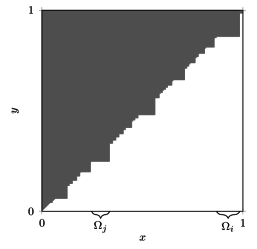
(b) A representation of the kernel $\mathrm{k}^{\prime}=\sum_{i\in I}\mathrm{k}_{i}$ with the white zone included in $\{\mathrm{k}^{\prime}=0\}$.

Figure 3. Example of a kernel $\mathrm{k}$ on $\Omega=[0,1]$ and the kernel $\mathrm{k}^{\prime}=\sum_{i\in I}\mathrm{k}_{i}$, with $\mathrm{k}_{i}(x,y)=\mathbb{1}_{\Omega_{i}}(x)\,\mathrm{k}(x,y)\,\mathbb{1}_{\Omega_{i}}(y)$ and $(\Omega_{i},i\in I)$ the non-zero atoms. We have $\operatorname{Spec}(T_{\mathrm{k}})=\operatorname{Spec}(T_{\mathrm{k}^{\prime}})$ as well as $R_{e}[T_{\mathrm{k}}]=R_{e}[T_{\mathrm{k}^{\prime}}]$.

We say the kernel $\mathrm{k}$ is monatomic if there exists a unique non-zero atom ($\sharp I=1$), and the kernel is quasi-irreducible if it is monatomic, with non-zero atom say $\Omega_{\mathrm{a}}$, and $\mathrm{k}\equiv 0$ outside $\Omega_{\mathrm{a}}\times\Omega_{\mathrm{a}}$. The quasi-irreducible property is the usual extension of the irreducible property in the setting of symmetric kernels; and the monatomic property is the natural generalization to non-symmetric kernels. We represented in Figure 4(a) a monatomic kernel $\mathrm{k}$ with non-zero atom say $\Omega_{\mathrm{a}}$ and in Figure 4(b) the quasi-irreducible kernel $\mathrm{k}_{\mathrm{a}}=\mathbb{1}_{\Omega_{\mathrm{a}}}\mathrm{k}\mathbb{1}_{\Omega_{\mathrm{a}}}$ with the same atom; the set $\Omega$ being “nicely ordered” so that the representation of the kernels are upper triangular and the set $\Omega_{\mathrm{i}}$ in Figure 4(a) corresponds to the sub-population infected by the atom $\Omega_{\mathrm{a}}$.

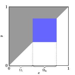
(a) A representation of a monatomic kernel.

(b) A representation of a quasi-irreducible kernel.

Figure 4. Example of kernels $\mathrm{k}$ and $\mathrm{k}_{\mathrm{a}}$ of a monatomic integral operator $T_{\mathrm{k}}$ and the quasi-irreducible integral operator $T_{\mathrm{a}}=T_{\mathrm{k}_{\mathrm{a}}}$ on $\Omega=[0,1]$, with non-zero atom $\Omega_{\mathrm{a}}$. The kernels are zero on the white zone and are irreducible when restricted to the blue zone.

5.2. The anti-Pareto frontier for irreducible and monatomic kernels

We prove in the next result that for positive and/or irreducible kernels, the gaps in Table 1 may essentially be filled. We illustrate these properties in Figure 5 by plotting the typical Pareto and anti-Pareto frontiers for irreducible kernels and positive kernels. In order to avoid the degenerate irreducible kernel, we shall consider a non-zero kernel $\mathrm{k}$, that is a kernel such that $\mathrm{k}(\Omega,\Omega)$ is positive.

Proposition 5.1 (Consequences of irreducibility).

Suppose that the cost function $C$ is continuous decreasing with $C(\mathbb{1})=0$ and consider the loss function $R_{e}=R_{e}[\mathrm{k}]$, with $\mathrm{k}$ a finite double norm irreducible non-zero kernel. Then, we have the following properties:

1. 1. $R_{0}>0$.

   2. The function $R_{e}^{\star}$ is continuous, decreasing on $[c^{\star},c_{\max}]$.

   3. The function $C^{\star}$ is continuous and decreasing on $[0,R_{0}]$.

   4. We have $C^{\star}\circ R_{e}^{\star}(c)=c$ for $c\in[c^{\star},c_{\max}]$.

   5. The set $\mathcal{P}^{\mathrm{Anti}}$ is compact (for the weak-* topology), $\mathcal{F}^{\mathrm{Anti}}$ is connected and compact, and:

      $$\mathcal{F}^{\mathrm{Anti}}=\{(c,R_{e}^{\star}(c))\,\colon\,c\in[c^{\star},c_{\max}]\}.$$

   6. $c^{\star}=0$.

2. If furthermore $\mathrm{k}>0$ a.e., then we also have:

   1. $c_{\star}=c_{\max}$.

   2. The strategy $\mathbb{1}$ (resp. $\mathbb{0}$) is the only Pareto optimal as well as the only anti-Pareto optimal strategy with cost $c=0$ (resp. $c=1$).

Proof.

According to [schaefer_banach_1974, Theorem V.6.6], if $\mathrm{k}$ is an irreducible kernel with finite double norm, then, as $\mathrm{k}$ is non-zero, we have $R_{0}=R_{0}[\mathrm{k}]>0$. This gives i ia.

The other items follow from various results from [ddz-theo]: Assumptions 3 and 6 from that paper hold, as well as Assumption 7, thanks to [ddz-theo, Lemma 5.14]. In the notation of [ddz-theo], as $\Omega_{\mathrm{a}}=\Omega$, we get $c^{\star}=C(\mathbb{1})=0$. We conclude using [ddz-theo, Proposition 5.9] that items i ib- ie hold.

We now assume that $\mathrm{k}>0$ a.e. As $c^{\star}=0$, we deduce that the strategy $\mathbb{1}$ is anti-Pareto optimal. As $C$ is decreasing, we also get that the strategy $\mathbb{1}$ is Pareto optimal.

Let $\eta\in\Delta$ be different from $\mathbb{0}$. The kernel $\mathrm{k}\eta$ restricted to the set of positive $\mu$-measure $\{\eta>0\}$ is positive, thus the kernel $\mathrm{k}\eta$ restricted to $\{\eta>0\}$ is positive. It is therefore irreducible and its spectral radius is positive, so $R_{e}(\eta)>0$. This also readily implies that $c_{\star}=c_{\max}$ and that the strategy $\mathbb{0}$ is Pareto optimal. As $C$ is decreasing, we also get that the strategy $\mathbb{0}$ is anti-Pareto optimal. ∎

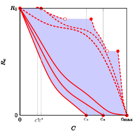
(a) General kernel.

(b) Monatomic kernel.

(c) Irreducible kernel.

(d) Kernel strictly positive almost surely.

Figure 5. Generic aspect of the feasible region (light blue), the Pareto frontier (thick red line) and the anti Pareto frontier (dashed red line) for the loss function $R_{e}[\mathrm{k}]$, with kernel $\mathrm{k}$, and a continuous decreasing cost function $C$.

We now state the properties of the anti-Pareto frontiers for monatomic kernel.

Corollary 5.2 (Consequences of monatomicity).

Suppose that the cost function $C$ is continuous decreasing with $C(\mathbb{1})=0$ and consider the loss function $R_{e}=R_{e}[\mathrm{k}]$, with $\mathrm{k}$ a finite double norm monatomic kernel with non-zero atom $\Omega_{\mathrm{a}}$. Then, Properties i ia-ie of Proposition 5.1 hold. The strategy $\mathbb{1}_{\Omega_{\mathrm{a}}}$ is anti-Pareto optimal with cost $c^{\star}=C(\mathbb{1}_{\Omega_{\mathrm{a}}})$.

Proof.

According to [ddz-theo, Lemma 5.14], we get that $R_{0}$ is positive and $c^{\star}=C(\mathbb{1}_{\Omega_{\mathrm{a}}})$. The other results are proved as in Proposition 5.1. ∎

Using the properties of the anti-Pareto frontiers stated in Proposition 5.1 for positive kernels and in Corollary 5.2 for monatomic kernel, we plotted in Figure 5 the typical Pareto and anti-Pareto frontiers for a general kernel (notice the anti-Pareto frontier is not connected a priori), a monatomic kernel (notice the anti-Pareto frontier is connected), and a positive kernel.

5.3. Creating a cordon sanitaire is not the worst idea

We say a strategy $\eta\in\Delta$ is a cordon sanitaire or disconnecting (for the kernel $\mathrm{k}$) if $\eta\neq\mathbb{0}$ and the kernel $\mathrm{k}$ restricted to the set $\{\eta>0\}$ is not connected (that is, not irreducible). Let us first give a few elementary comments on disconnecting strategies.

• The strategy $\eta=\mathbb{1}$ is disconnecting if and only if $\mathrm{k}$ is not connected.

• Disconnection only depends on fully vaccinated individuals: A strategy $\eta$ is disconnecting if and only if the strategy $\mathbb{1}_{\{\eta>0\}}$ is disconnecting.

• If $\mathrm{k}>0$, then there is no disconnecting strategy.

• If $\eta\neq\mathbb{0}$ is a strategy such that $\mathrm{k}=0$ a.e. on $\{\eta>0\}^{2}$, then $\eta$ is disconnecting.

The next proposition states that if the strategy $\eta$ is anti-Pareto optimal for a kernel $\mathrm{k}$ and non zero, then the kernel $\mathrm{k}$ restricted to $\{\eta>0\}$ is irreducible. Let us remark that in general this implication is not an equivalence.

Proposition 5.3 (A cordon sanitaire is never the worst idea).

Suppose that the cost function $C$ is continuous decreasing and consider the loss function $R_{e}[\mathrm{k}]$, with $\mathrm{k}$ a finite double norm kernel on $\Omega$ such that $R_{0}[\mathrm{k}]>0$. Then, a disconnecting strategy is not anti-Pareto optimal.

In the non-oriented cycle graph from Example 1.1, this property is illustrated in Figure 1 as the disconnecting strategy “one in $4$” is not anti-Pareto optimal; see Figure 2

Proof.

Let $\eta$ be a disconnecting strategy, and thus $\eta\neq\mathbb{0}$. Since $\eta$ is disconnecting, that is, $\mathrm{k}$ restricted to $\{\eta>0\}$ is not irreducible, we deduce there exists $A,B\in\mathscr{F}$ such that $\mu(A)>0$, $\mu(B)>0$, $(\mathrm{k}\eta)(B,A)=0$ and a.e. $A\cup B=\{\eta>0\}$ and $A\cap B=\emptyset$. We deduce from [ddz-Re, Equation (29)] where we can replace $\mathrm{k}$ by $\mathrm{k}\eta$ that:

(25) $$R_{e}[\mathrm{k}\eta](\mathbb{1}_{A}+\mathbb{1}_{B})=\max\left(R_{e}[\mathrm{k}\eta](\mathbb{1}_{A}),R_{e}[\mathrm{k}\eta](\mathbb{1}_{B})\right).$$

First assume that $R_{e}[\mathrm{k}\eta](\mathbb{1}_{A})\geq R_{e}[\mathrm{k}\eta](\mathbb{1}_{B})$, so that:

$$R_{e}[\mathrm{k}](\eta)=R_{e}[\mathrm{k}\eta](\mathbb{1}_{\{\eta>0\}})=R_{e}[\mathrm{k}\eta](\mathbb{1}_{A}+\mathbb{1}_{B})=R_{e}[\mathrm{k}\eta](\mathbb{1}_{A}).$$

For $\theta\in[0,1]$, define the strategy $\eta_{\theta}=\eta\mathbb{1}_{A}+\theta\eta\mathbb{1}_{B}$. We deduce that:

$$R_{e}[\mathrm{k}](\eta_{\theta})=R_{e}[\mathrm{k}\eta_{\theta}](\mathbb{1}_{A}+\mathbb{1}_{B}) =\max(R_{e}[\mathrm{k}\eta_{\theta}](\mathbb{1}_{A}),R_{e}[\mathrm{k}\eta_{\theta}](\mathbb{1}_{B}))$$

$$=\max(R_{e}[\mathrm{k}\eta](\mathbb{1}_{A}),\theta R_{e}[\mathrm{k}\eta](\mathbb{1}_{B}))$$

$$=R_{e}[\mathrm{k}\eta](\mathbb{1}_{A})$$

$$=R_{e}[\mathrm{k}](\eta),$$

where we used (25) with $\eta$ replaced by $\eta_{\theta}$ for the second equality as $(\mathrm{k}\eta_{\theta})(B,A)=0$, and the homogeneity of the spectral radius in the third. Thus, the map $\theta\mapsto R_{e}[\mathrm{k}](\eta_{\theta})$ is constant on $[0,1]$. Since $\mu(B)>0$ and $C$ is decreasing, we get that $\theta\mapsto C(\eta_{\theta})$ is decreasing. This implies that $\eta_{\theta}$ is worse than $\eta$ for any $\theta\in[0,1)$, and thus $\eta$ is not anti-Pareto optimal.

The case $R_{e}[\mathrm{k}\eta](\mathbb{1}_{B})\geq R_{e}[\mathrm{k}\eta](\mathbb{1}_{A})$ is handled similarly. ∎

Remark 5.4.

If the kernel $\mathrm{k}$ is irreducible and non-zero, then the upper boundary of the set of outcomes $\mathbf{F}$ is the anti-Pareto frontier; see Figure 5(c) for instance. We deduce from Proposition 5.3 that if $\eta_{0}$ is a disconnecting strategy, then we have that $R_{e}[\mathrm{k}](\eta_{0})$ is strictly less that $\sup\{R_{e}[\mathrm{k}](\eta)\,\colon\,C(\eta)=C(\eta_{0})\}$.

However, if the kernel $\mathrm{k}$ is not irreducible, then the trivial strategy $\mathbb{1}$ is disconnecting. Furthermore, the upper boundary of the set of outcomes $\mathbf{F}$ is not reduced to the anti-Pareto frontier; see Figure 5(a) for instance. In fact, there exists disconnecting strategies that are not anti-Pareto optimal, but whose outcomes lie on the flat parts of the upper boundary of $\mathbf{F}$. In particular, such strategies have the worst loss given their cost. However, it is not difficult to check that they do not disconnect further than the trivial strategy $\mathbb{1}$.

5.4. Pareto and anti-Pareto frontiers for reducible kernels

Let us now assume that the kernel $\mathrm{k}$ is “truly reducible”, in the sense that it has at least two non-zero atoms, and thus $R_{0}=R_{0}[\mathrm{k}]>0$. We will see in this section how to effectively reduce the study of the global optimization problem to a study of the optimization problem on each non-zero atom. Recall the collection of non-zero atoms $(\Omega_{i},i\in I)$ defined in Section 5.1 and the corresponding quasi-irreducible kernels $(\mathrm{k}_{i},i\in I)$ in (24). By construction, the kernel $\mathrm{k}_{i}$ has a finite double norm and $R_{0}[\mathrm{k}_{i}]>0$.

We now describe two ways of restricting the problem to an atom. For the kernel $\mathrm{k}_{i}$ and the loss function $R_{e}[\mathrm{k}_{i}]$, the atom is still viewed as a part of the larger population $\Omega$. As such, the vaccination strategies that agree on $\Omega_{i}$ but differ on $\Omega_{i}^{c}$ will have the same loss, but their costs may differ. For $i\in I$ and $\eta\in\Delta$, we set similarly:

$$\eta_{i}=\eta\mathbb{1}_{\Omega_{i}}.$$

We consider the loss $R_{e}[\mathrm{k}_{i}]$ and the corresponding optimal loss function $R^{\star}_{i}$ defined on $[0,c_{\max}]$ and optimal cost function $C^{\star}_{i}$ and $C_{i,\star}$. For convenience the functions $C^{\star}_{i}$ and $C_{i,\star}$ which are defined on $[0,R_{0}[\mathrm{k}_{i}]]$ are extended to $[0,R_{0}]$ by letting them be equal to 0 on $(R_{0}[\mathrm{k}_{i}],R_{0}]$.

Another point of view is to restrict the kernel and vaccination strategies to the atom, and study it intrinsically, in isolation. Quantities and functions defined by this intrinsic approach will be denoted by bold letters. In particular $\bm{\mathrm{k}}_{i}:\Omega_{i}^{2}\to\mathbb{R}$ is the kernel $\mathrm{k}$ (and $\mathrm{k}_{i}$) restricted to $\Omega_{i}$; it is irreducible and non-zero by construction and $R_{0}[\bm{\mathrm{k}}_{i}]$ is a simple positive eigenvalue of the corresponding integral operator. If $\eta$ is a vaccination strategy, then $\bm{\eta}_{i}$ is its restriction to $\Omega_{i}$. By construction, we have for all $\eta\in\Delta$:

$$R_{e}[\mathrm{k}_{i}](\eta)=R_{e}[\mathrm{k}_{i}](\eta_{i})=R_{e}[\bm{\mathrm{k}}_{i}](\bm{\eta}_{i}).$$

If $\bm{\eta}$ is a $[0,1]$-valued measurable function defined on $\Omega_{i}$, we define its extension $\eta$ on $\Omega$ (corresponding to no vaccinations outside $\Omega_{i}$) and its cost by:

$$\eta=\begin{cases}\bm{\eta}&\text{on $\Omega_{i}$}\\ \mathbb{1}&\text{on $\Omega_{i}^{c}$}\\ \end{cases}\quad\quad\text{and}\quad\bm{C}_{i}(\bm{\eta})=C(\eta).$$

The optimization problems (17) and (19) may now be stated on each $\Omega_{i}$ for the kernel $\bm{\mathrm{k}}_{i}$, the loss $R_{e}[\bm{\mathrm{k}}_{i}]$ and the cost $\bm{C}_{i}$: denote by $\bm{C}_{i,\star}$ and $\bm{C}_{i}^{\star}$ the corresponding optimal cost functions, and extend them to $[0,R_{0}]$ by letting them be equal to 0 on $(R_{0}[\mathbf{k}_{i}],R_{0}]$. In particular, by construction, $\bm{C}_{i,\star}$ is equal to $C_{i,\star}$. However, there is no relation in general between $\bm{C}_{i}^{\star}$ and $C_{i}^{\star}$. Nevertheless, it is possible to establish such a relation when the cost is extensive. Recall once more that for a vaccination strategy $\eta$, the proportion of vaccinated individuals of trait $x$ is given by $1-\eta(x)$. Thus, two vaccination strategies $\eta$ and $\eta^{\prime}$ target disjoint subsets of the population if $\eta\vee\eta^{\prime}=\mathbb{1}$.

Definition 5.5 (Extensivity).

Let $C$ be a continuous decreasing cost function with $C(\mathbb{1})=0$. The cost $C$ is called extensive if vaccinating disjoint subsets of the population is additive:

$$C(\eta\wedge\eta^{\prime})=C(\eta)+C(\eta^{\prime})\quad\text{for all $\eta,\eta^{\prime}\in\Delta$ such that $\eta\vee\eta^{\prime}=\mathbb{1}$}.$$

If the continuous decreasing cost function $C$ is extensive, then we get for all $\eta\in\Delta$ that:

(26) $$C(\eta)=\sum_{i\in I}C(\eta_{i}+\mathbb{1}_{\Omega_{i}^{c}})=\sum_{i\in I}\bm{C}_{i}(\bm{\eta}_{i}),$$

since all the vaccinations $\eta_{i}+\mathbb{1}_{\Omega_{i}^{c}}$ target pairwise disjoint subsets of the population.

Remark 5.6 (Affine costs are extensive).

If the cost function takes the form

$$C(\eta)=c_{\max}-\int_{\Omega}\phi(\eta(x),x)\,\mu(dx)$$

where $\phi\,\colon\,[0,1]\times\Omega\to\mathbb{R}_{+}$ is measurable and non-decreasing in its first variable, then $C$ is extensive. In particuar, the affine cost functions considered in Proposition 4.1 are extensive.

We are now ready to state the reduction result, which in particular implies that if the cost function is extensive, then the (anti-)Pareto frontier of the full model may be constructed from the family of (anti-)Pareto frontiers of each atom.

Proposition 5.7 (Reduction to atoms).

Let $\mathrm{k}$ be a kernel with finite double norm on $\Omega$, such that $R_{0}=R_{0}[\mathrm{k}]>0$. Suppose that the cost function $C$ is continuous decreasing with $C(\mathbb{1})=0$.

1. Decomposition of the loss. For any $\eta\in\Delta$, we have:

   (27) $$R_{e}[\mathrm{k}](\eta)=\max_{i\in I}R_{e}[\mathrm{k}](\eta\mathbb{1}_{\Omega_{i}})=\max_{i\in I}R_{e}[\mathrm{k}_{i}](\eta_{i})=\max_{i\in I}R_{e}[\bm{\mathrm{k}}_{i}](\bm{\eta}_{i}).$$

2. Anti-Pareto optimal strategies. For all $\ell\in[0,R_{0}]$ and $\eta\in\Delta$, the following two properties are equivalent:

   1. The strategy $\eta$ is anti-Pareto optimal with $R_{e}[\mathrm{k}](\eta)=\ell$.

   2. There exists $j\in\mathrm{argmax}_{i\in I}\,C_{i}^{\star}(\ell)$ such that $\eta=0$ on $\Omega_{j}^{c}$ and $\eta=\bm{\eta}_{j}$ on $\Omega_{j}$, where $\bm{\eta}_{j}$ is anti-Pareto optimal for $\bm{\mathrm{k}}_{j}$ on $\Omega_{j}$ and cost function $\bm{C}_{i}$ with $R_{e}[\bm{\mathrm{k}}_{j}](\bm{\eta}_{j})=\ell$.

   Besides, we have:

   (28) $$R_{e}^{\star}=\max_{i\in I}\,R^{\star}_{i}\quad\text{on $[0,c_{\max}]$}\quad\text{and}\quad C^{\star}=\max_{i\in I}\,C^{\star}_{i}\quad\text{on $[0,R_{0}]$}.$$

   Furthermore, if the cost function $C$ is extensive, then for all $i\in I$, we have:

   $$C_{i}^{\star}=\bm{C}_{i}^{\star}+C(\mathbb{1}_{\Omega_{i}}).$$

3. Pareto optimal strategies when the cost function is extensive. Suppose that the cost function $C$ is extensive. For all $\ell\in[0,R_{0}]$ and $\eta\in\Delta$, the following two properties are equivalent:

   1. The strategy $\eta$ is Pareto optimal with $R_{e}[\mathrm{k}](\eta)=\ell$.

   2. On $(\bigcup_{i\in I}\Omega_{i})^{c}$, $\eta=1$ and, for all $i\in I$, $\eta$ restricted to $\Omega_{i}$, say $\bm{\eta}_{i}$, is Pareto optimal for $\bm{\mathrm{k}}_{i}$ on $\Omega_{i}$ and cost function $\bm{C}_{i}$ with $R_{e}[\bm{\mathrm{k}}_{i}](\bm{\eta}_{i})=\min(\ell,R_{0}[\bm{\mathrm{k}}_{i}])$ (and thus $\bm{\eta}_{i}=\mathbb{1}$ if $R_{0}[\bm{\mathrm{k}}_{i}]\leq\ell$).

   Besides, we have:

   $$C_{\star}=\sum_{i\in I}\bm{C}_{i,\star}.$$

Remark 5.8 (Additional consequences).

From (21) and the second part of (28), we get that the anti-Pareto frontier is given by:

$$\mathcal{F}^{\mathrm{Anti}}=\left\{\left(\max_{i\in I}C_{i}^{\star}(\ell),\ell)\right)\,\colon\,\ell\in[0,R_{0}]\right\}.$$

We deduce from Point ii that the maximal cost of totally inefficient strategies is given by:

$$c^{\star}:=C^{\star}(R_{0})=\max_{i\in I}\{C(\mathbb{1}_{\Omega_{i}})\,\colon\,R_{0}[\mathrm{k}_{i}]=R_{0}[\mathrm{k}]\}.$$

According to [ddz-Re, Remark 5.1(v)] the number of atoms $\Omega_{i}$ such that $R_{0}[\mathrm{k}_{i}]=R_{0}[\mathrm{k}]$ is equal to the algebraic multiplicity of $R_{0}$ for $T_{\mathrm{k}}$.

As any Pareto optimal strategy is larger than $\mathbb{1}_{(\bigcup_{i\in I}\Omega_{i})^{c}}$ according to Point iii, we get an upper bound for the minimal cost which ensures that no infection occurs at all:

$$c_{\star}=C_{\star}(0)\leq C(\eta)\quad\text{with}\quad\eta=\mathbb{1}-\sum_{i\in I}\mathbb{1}_{\Omega_{i}}.$$

Remark 5.9.

If $R_{0}[\mathrm{k}]>0$ and $\mathrm{k}$ is not monatomic, then Assumption 7 in [ddz-theo] (that is any local maximum of the loss function is also a global maximum) may or may not be satisfied for the loss function ${R_{e}}=R_{e}[\mathrm{k}]$; this can happen even in a two homogeneous populations model. In the former case the function $C^{\star}$ is continuous and the anti-Pareto frontier is connected, whereas in the latter case the function $C^{\star}$ may have jumps and then the anti-Pareto frontier has more than one connected component.

Proof of Proposition 5.7.

Let $\mathrm{k}$ be a finite double norm kernel on $\Omega$ such that $R_{0}=R_{0}[\mathrm{k}]>0$. Set $\Omega_{0}=\Omega\setminus\cup_{i\in I}\Omega_{i}$. For $i\in I$ and $\eta\in\Delta$, we set $\eta_{i}=\eta\mathbb{1}_{\Omega_{i}}$.

According to (24) and since $R_{e}[\mathrm{k}_{i}](\eta)=R_{e}[\mathrm{k}_{i}](\eta_{i})=R_{e}[\mathrm{k}](\eta_{i})$, we can decompose $R_{e}[\mathrm{k}]$ according to the quasi-irreducible components $(\mathrm{k}_{i},i\in I)$ of $\mathrm{k}$ to get that for $\eta\in\Delta$:

(29) $$R_{e}[\mathrm{k}](\eta)=\max_{i\in I}R_{e}[\mathrm{k}_{i}](\eta)=\max_{i\in I}R_{e}[\mathrm{k}_{i}](\eta_{i})=\max_{i\in I}R_{e}[\mathrm{k}](\eta_{i}).$$

Then use that $\bm{\mathrm{k}}_{i}$ is the restriction of $\mathrm{k}_{i}$ to $\Omega_{i}$ to get Point i.

We now prove Point ii. Equation (29) and the definition of $R_{e}^{\star}$ readily implies that $R_{e}^{\star}=\max_{i\in I}\,R^{\star}_{i}$, which gives the first part of (28).

We prove that properties iia and iib are equivalent. The case $\ell=0$ being trivial, we only consider $\ell\in(0,R_{0}]$. Let $\eta$ be a strategy such that $R_{e}[\mathrm{k}](\eta)=\ell$. According to i, there exists $j$ such that $R_{e}[\mathrm{k}](\eta)=R_{e}[\mathrm{k}](\eta_{j})$. Since $\ell>0$, we get that $\eta_{j}$ is not equal to $\mathbb{0}$. Hence, we get:

$$C(\eta)\leq\inf_{i\in I}C(\eta_{i})\leq C(\eta_{j})\leq C^{\star}_{j}(\ell)\leq\sup_{i\in I}C^{\star}_{i}(\ell)\leq C^{\star}(\ell),$$

where:

1. the first and second inequalities become equalities if and only if $\eta_{i}=\mathbb{0}$ for all $i\neq j$ because $C$ is decreasing;

2. the third inequality is an equality if and only if $\bm{\eta}_{j}$ is anti-Pareto optimal (see Table 1);

3. the last inequality follows from the fact that $R_{e}[\mathrm{k}_{i}](\eta_{i})=R_{e}[\mathrm{k}](\eta_{i})$ for all $i\in I$.

Hence, Property iia is equivalent to the following equalities:

(30) $$C^{\star}_{j}(\ell)=C(\eta_{j})=C(\eta)=C^{\star}(\ell).$$

which is equivalent to Property iib. In particular, it follows from the existence of the anti-Pareto optimal strategy that $\sup_{i\in I}C^{\star}_{i}$ is in fact a $\max$.

We now prove that $C_{i}^{\star}=\bm{C}_{i}^{\star}+C(\mathbb{1}_{\Omega_{i}})$ for all $i\in I$ in case $C$ is extensive. Note that the optimal cost $\bm{C}_{i}^{\star}$, defined in terms of the restricted kernel $\bm{\mathrm{k}}_{i}$, and which may be viewed as intrinsic on $\Omega_{i}$, differs from the cost $C_{i}^{\star}$, defined on the “extrinsic” kernel $\mathrm{k}_{i}$ defined on the whole space $\Omega$. Let $\ell\in[0,R_{0}]$. The worst vaccinations on the whole space clearly consist in vaccinating everyone outside $\Omega_{i}$ and vaccinating in the worst possible way inside $\Omega_{i}$, that is, if $\eta$ is anti-Pareto optimal for the kernel $\mathrm{k}_{i}$ with loss $\ell\in[0,R_{0}]$ and cost $C(\eta)$, then $\eta=\bm{\eta}_{i}\mathbb{1}_{\Omega_{i}}$, where $\bm{\eta}_{i}$ is anti-Pareto optimal for the kernel $\bm{\mathrm{k}_{i}}$ with loss $\ell$ and cost $\bm{C}_{i}^{\star}(\ell)=\bm{C}_{i}(\bm{\eta}_{i})$. Set $\eta^{\prime}=\eta+\mathbb{1}_{\Omega_{i}^{c}}$ and $\eta^{\prime\prime}=\mathbb{1}_{\Omega_{i}}$ so that $\eta=\eta^{\prime}\vee\eta^{\prime\prime}=\mathbb{1}$. By definition of $\bm{C}_{i}$, we have $C(\eta^{\prime})=\bm{C}_{i}(\bm{\eta}_{i})$. Since $C$ is extensive, we get:

$$C^{\star}_{i}(\ell)=C(\eta)=C(\eta^{\prime})+C(\eta^{\prime\prime})=\bm{C}_{i}(\bm{\eta}_{i})+C(\mathbb{1}_{\Omega_{i}})=\bm{C}_{i}^{\star}(\ell)+C(\mathbb{1}_{\Omega_{i}}).$$

Point iii follows directly from Point i and the the following decomposition of $C$ as an extensive function:

(31) $$C(\eta)=\sum_{i\in I}\bm{C}_{i}(\bm{\eta}_{i}).\qed$$