Blind and Channel-agnostic Equalization
Using Adversarial Networks

Abstract

Due to the rapid development of autonomous driving, the Internet of Things and streaming services, modern communication systems have to cope with varying channel conditions and a steadily rising number of users and devices. This, and the still rising bandwidth demands, can only be met by intelligent network automation, which requires highly flexible and blind transceiver algorithms. To tackle those challenges, we propose a novel adaptive equalization scheme, which exploits the prosperous advances in deep learning by training an equalizer with an adversarial network. The learning is only based on the statistics of the transmit signal, so it is blind regarding the actual transmit symbols and agnostic to the channel model. The proposed approach is independent of the equalizer topology and enables the application of powerful neural network based equalizers. In this work, we prove this concept in simulations of different—both linear and nonlinear—transmission channels and demonstrate the capability of the proposed blind learning scheme to approach the performance of non-blind equalizers. Furthermore, we provide a theoretical perspective and highlight the challenges of the approach.

I Introduction

The digital transformation and the advent of video streaming platforms brought up a strong demand for high-speed and highly flexible communication systems. Along with the rapid development of autonomous driving, the Internet of Things and Industry 4.0, intelligent automation becomes highly important for modern communication networks to adapt quickly to varying channel conditions. This adaptation should not only be performed quickly but also fully autonomously to enable the design of fast, low-cost and low-latency transmission systems for a broad range of applications, where no further expert knowledge or extensive parameter searches are required during run-time. This requires high flexibility of the signal processing algorithms; however, state-of-the-art algorithms usually assume certain channel models or transmission characteristics in their training objective. The constant modulus algorithm (CMA) [1] and its derivatives, e.g., assume symmetric single-level modulation formats. Other algorithms assume specific channels, e.g., the additive white Gaussian noise (AWGN) channel or the nonlinear optical channel described by the Manakov equation. Channel-agnostic algorithms, however, can also be used if the channel model is unknown or if it deviates significantly from the real channel. Furthermore, modern state-of-the-art transmission systems often rely on data-aided (or pilot-based) signal processing algorithms, however, the resulting overhead limits the achievable net bit rate significantly. Hence, there is a strong demand on blind and flexible transceiver algorithms.

In this paper, we propose a novel blind and channel-agnostic approach to train an equalizer with an adversarial network, while, to the best of our knowledge, there is no blind state-of-the-art equalizer which is fully agnostic to the channel model. Our approach is based on generative adversarial networks [2], which represent an unsupervised learning concept based on two neural networks, the generator and the discriminator, where both are trained jointly in a zero-sum game. The concept is commonly used in image processing and computer vision, e.g., to increase the amount of training data [3] or for generating realistic artificial photographs [4, 5]. In recent years, multiple works focused on applying the GAN concept to communication systems. The most common use-case is autonomous channel modeling, where the GAN is trained on raw measurements to obtain an appropriate and differentiable channel model [6, 7, 8, 9]. For instance, a GAN is used to predict unknown channel transition probabilities, which are further utilized by the Viterbi algorithm for channel-independent maximum-likelihood sequence detection (MLSD) [7]. However, the approach still faces the common issues of MLSD, e.g., exponentially-increasing complexity with increasing channel memory, which makes it impractical for many realistic communication channels.

Contrarily, we focus on a different approach which is more similar to [10], where an error correcting decoder is trained with adversarial networks. Instead of using the generator to create new data samples from noise as input, as in most GAN applications for channel modelling, [10] feeds the generator with the received noisy codewords. The generator serves as decoder to recover the transmitted codewords and is trained together with the adversarial discriminator, which tries to distinguish between the decoder output and valid reference codewords. In a similar way, instead of recovering noisy codewords, we focus on equalizing a received sequence of symbols, which is not only corrupted by noise but also distorted by potential nonlinearities and effects with memory, e.g., inter-symbol interference (ISI). However, the distortions cause our problem to be much more demanding than the recovery of noisy codewords. In this work, we propose a concept to utilize the novel GAN approach for blind and channel-agnostic equalization, and prove it in simulations of these demanding conditions. Compared to [10], we use the generator as equalizer (instead of decoder), feed it with the received sequence and train it with an adversarial discriminator based on reference sequences. In fact, we only require knowledge of the transmitted sequences’ statistics to draw new reference sequences at the receiver, but do not need any supervision or channel model in training. Hence, the novel training scheme is blind, channel-agnostic and independent of the equalizer topology. We demonstrate its high flexibility and introduce concepts to improve training along with appropriate topologies based on both linear equalizers and NNs. Furthermore, we analyze the approach from a theoretical perspective and show that it is potentially able to outperform state-of-the-art equalizers.

II Concept of Generative Adversarial Networks

In this work, we exploit the concept of GANs to train an equalizer (generator) using an adversarial discriminator.

A GAN consists of two individual (parametric) functions—generator $G$ and discriminator $D$—which are usually represented by NNs and trained in an adversarial manner [2]. Precisely, they play a minimax-game, i.e., optimize the value function

$$\begin{split}\min_{G}\,\max_{D}\,V(D,G)&=\operatorname{\mathbb{E}}_{\bm{x}^{\prime}\sim p\left(\bm{x}\right)}\left\{\log{D\left(\bm{x}^{\prime}\right)}\right\}\\ &\qquad+\operatorname{\mathbb{E}}_{\bm{y}\sim p\left(\bm{y}\right)}\left\{\log\left(1-D\left(G\left(\bm{y}\right)\right)\right)\right\}\end{split}$$

with $\operatorname{\mathbb{E}}_{\bm{y}\sim p\left(\bm{y}\right)}\left\{\cdot\right\}$ being the expectation with respect to $p\left(\bm{y}\right)$ and $\bm{x}^{\prime}$ being reference samples drawn from the desired probability density function (pdf) $p\left(\bm{x}\right)$. In simple words, $G$ tries to “fool” the discriminator by generating an output—usually out of noise as input—which resembles the reference samples $\bm{x}^{\prime}$, while $D$—which outputs a scalar representing the probability of its input being a reference sample—tries to discriminate correctly between generator output $G\left(\bm{y}\right)$ and reference samples $\bm{x}^{\prime}$.

Goodfellow et al. showed that the minimax-game’s global optimum is at $p\left(\bm{z}\right)=p\left(\bm{x}\right)$ (with $\bm{z}=G\left(\bm{y}\right)$) and that their proposed training [2, Algorithm 1] converges to this optimum, if “$G$ and $D$ have enough capacity and, at each step of Algorithm 1, the discriminator is allowed to reach its optimum given $G$” [2]. Importantly, $G$ and $D$ are updated blindly (without supervision) using any gradient-based learning rule, e.g. [11], with the aid of the reference symbols, which can be generated at the receiver.

III GAN-based Equalization

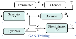
Figure 1: Structure of the proposed GAN-based blind equalization approach. Data symbols $\bm{x}$ are transmitted over an unknown communication channel to a receiver. Only the colored components belong to the receiver and the components in the dotted box are specific to the GAN approach. The generator $G$ is the equalizer, $\bm{x}^{\prime}$ are reference symbols (generated at the receiver) and $\hat{\bm{x}}$ are the recovered symbols.

In our novel approach, we utilize the GAN for blind channel-agnostic equalization by considering the equalizer as generator $G$ and introducing an additional discriminator $D$ for adversarial learning, as depicted in Fig. 1.

Since the proposed equalizer is channel-agnostic, we assume a general communication system where the transmitted vector $\bm{x}$, consisting of symbols $x_{i}\in\mathcal{A}$ from an alphabet $\mathcal{A}=\left\{A_{1}\ldots A_{M}\right\}$, is distorted by an unknown channel and results in a received vector $\bm{y}$.

Instead of inputting noise to the generator, as in most GAN implementations, we pass the received vector $\bm{y}$ to the generator to operate it like a conventional equalizer. The proposed approach allows various linear and nonlinear equalizer and discriminator topologies, so it is not limited to specific NNs; however, it has to be highlighted that the topologies determine the equalizer output $\bm{z}$ as well as the family of potential $p\left(\bm{z}\right)$, which can be generated by the equalizer. Hence, the topologies have to be chosen carefully.

III-A Training

$N_{\mathrm{TI}}$: Number of TIs;    $N$: Number of symbols per TI

$N_{\mathrm{d}}$: Number of discriminator updates per TI

$\mathcal{N}_{N}\left(\mu,\,\sigma^{2}\right)$: $N$-dimensional normal distribution with each dimension’s mean $\mu$ and variance $\sigma^{2}$

$\gamma_{\text{ch}}\left(\bm{x}\right)$: Function representing the channel distortions

$\sigma_{\mathrm{ref}}^{2}\left(i\right)$: Function returning the reference’s variance at the TI $i$

for ( $i=0$; $i<N_{\mathrm{TI}}$; $i\text{++}$ )

       /* Train Discriminator */

       for ( $j=0$; $j<N_{\mathrm{d}}$; $j\text{++}$ )

             /* Sample reference symbols */

             $\bm{x}^{\prime}\sim P\left(\bm{x}\right)+\mathcal{N}_{N}\left(0,\,\sigma_{\mathrm{ref}}^{2}\left(i\right)\right)$

             /* Sample channel output */

             $\bm{y}\sim\gamma_{\text{ch}}\left(\bm{x}\right)+\mathcal{N}_{N}\left(0,\,\sigma^{2}_{\mathrm{n}}\right)$ with $\bm{x}\sim p\left(\bm{x}\right)$

             /* Generate fake symbols */

             $\bm{z}=G(\bm{y})$

             /* Get predictions of D to calc loss */

             $\text{loss}_{\mathrm{D}}=\text{BCE}(D(\bm{x}^{\prime}),1)+\text{BCE}(D(\bm{z}),0)+\text{HWA}_{\mathrm{D}}$

             update parameters of $D$ based on $\text{loss}_{\mathrm{D}}$

            

      

      /* Train Generator */

       /* Get prediction for $\bm{z}$ and calc loss */

       $\text{loss}_{\mathrm{G}}=\text{BCE}(D(\bm{z}),1)+\text{HWA}_{\mathrm{G}}$

       update parameters of $G$ based on $\text{loss}_{\mathrm{G}}$

      

Algorithm 1 Training flow of the GAN-equalizer

In order to train the generator and discriminator, we make use of the non-saturating (NS)-GAN approach described in [2, 12], where the generator is trained by maximizing $\log{D\left(G\left(\bm{y}\right)\right)}$ instead of minimizing $\log\left(1-D\left(G\left(\bm{y}\right)\right)\right)$. This prevents the saturation of the generator loss function early in learning (when $G$ is poor, so $D$ can easily distinguish between $\bm{z}$ and $\bm{x}^{\prime}$) but has the same fixed point of $G$’s and $D$’s dynamics [2].

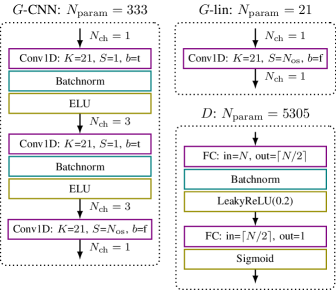
Figure 2: Topology of the generator $G$ (CNN and lin) and discriminator $D$ with kernel size $K$, stride $S$, oversampling factor $N_{\mathrm{os}}$, number of channels $N_{\mathrm{ch}}$, number of trainable parameters $N_{\mathrm{param}}$, and the bias $b$ being true (t) or false (f).

Additionally, we tackle the same issue by blurring $\bm{x}^{\prime}$ with Gaussian noise, whose variance $\sigma_{\mathrm{ref}}^{2}\left(i\right)$ decreases with the training iterations. As suggested in [12], we apply historical weight averaging (HWA) for both $G$ and $D$ to increase the training stability. Precisely, we penalize parameter updates with a large difference to the corresponding parameters’ moving average (MA) of the past 200 TIs.

The complete training flow is described in Algorithm 1. We use binary cross-entropy (BCE) loss for both the generator and the discriminator, and have two separate optimizers for $G$ and $D$. Thus, both can be trained with individual update rules and learning rates $\epsilon_{\mathrm{lr}}$. In this work, both use the Adam algorithm [11]. We train the models with $N_{\mathrm{d}}=2$, $N=100$ symbols per TI and apply a learning rate scheduler, which multiplies the learning rate by $0.3$ after predefined TIs steps.

III-B Topology

The structures of the NNs used to achieve the results presented in Sec. IV are illustrated in Fig. 2; however, we want to highlight that the approach itself is topology-independent and that we do not claim that the proposed structures are optimal. Yet, we performed an extensive design space exploration to find topologies of low complexity, which achieve satisfying results in our simulations. We leave further topology optimization for future research.

Precisely, we implemented two structures for the generator as depicted in Fig. 2: $G$-CNN is based on a convolutional neural network (CNN) and $G$-lin is based on a linear finite impulse response (FIR) filter. $G$-CNN is composed of three one-dimensional convolutional layers (conv1D) with, except for the last layer, batchnorm [13] and exponential linear unit (ELU) activation. The intermediate layers expand to three channels increasing the CNN’s expressive power and the last layer downsamples by a stride $S=N_{\mathrm{os}}$, where $N_{\mathrm{os}}$ is the oversampling factor in samples per symbol (sps). $G$-lin corresponds to $G$-CNN’s last layer, but only has one input and output channel. We use a uniform Glorot initialization in the first layer and Dirac in the remaining layers (as well as for $G$-lin), since we expect that this fits best to the final weight values. Again, we propose the optimization of the initializations as subject of future research.

The discriminator receives a sequence as input but has to output a scalar (probability), so we implemented this funnel-like shape with a two-layer fully connected (FC) NN as depicted in Fig. 2.

III-C Theoretical Perspective

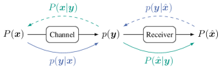
Figure 3: Simple system model and its corresponding pdfs and pmfs: transmitted vector $\bm{x}$, received vector $\bm{y}$ and recovered vector $\hat{\bm{x}}$ are realizations of random variable sequences $\{X_{k}\}$, $\{Y_{k}\}$ and $\{\hat{X}_{k}\}$.

Additionally to the rather practical deep learning perspective in the previous sections, in the following, we analyse the approach from a theoretical point of view. Therefore, we depict a general communication system as in Fig. 3. The transmitted vector $\bm{x}$ is a realization of the random variable sequence $\left\{X_{k}\right\}\sim P\left(\bm{x}\right)$, where $P\left(\bm{x}\right)$ is the corresponding probability mass function (pmf). The channel distorts $\bm{x}$ and, thus, transforms the random variable sequence $\left\{X_{k}\right\}$. If there is superimposed continuously-distributed noise, e.g., AWGN, the received symbols’ random variable sequence follows a pdf, i.e., $\left\{Y_{k}\right\}\sim p\left(\bm{y}\right)$.

The optimum decision is based on the maximum a posteriori (MAP) probability [14, Ch. 4.1]

$$P\left(\bm{x}|\bm{y}\right) =\frac{p\left(\bm{y}|\bm{x}\right)\cdot P\left(\bm{x}\right)}{p\left(\bm{y}\right)}\ ,$$

where the likelihood $p\left(\bm{y}|\bm{x}\right)$ describes the channel. If $p\left(\bm{y}|\bm{x}\right)$ is unknown, $P\left(\bm{x}|\bm{y}\right)$ is intractable to compute. Hence, Fig. 3 reveals that we have to find a receiver, which equalizes $\bm{y}$ such that

$$\frac{p\left(\bm{y}|\hat{\bm{x}}\right)\cdot P\left(\hat{\bm{x}}\right)}{p\left(\bm{y}\right)}=P\left(\hat{\bm{x}}|\bm{y}\right) \overset{!}{=}P\left(\bm{x}|\bm{y}\right)=\frac{p\left(\bm{y}|\bm{x}\right)\cdot P\left(\bm{x}\right)}{p\left(\bm{y}\right)}\;,$$

where $\hat{\bm{x}}$ is the output after equalizer and demapper. One possible solution for this problem is

$$p\left(\bm{y}|\hat{\bm{x}}\right)\overset{(i)}{=}p\left(\bm{y}|\bm{x}\right)\quad \text{and}\quad P\left(\hat{\bm{x}}\right)\overset{(ii)}{=}P\left(\bm{x}\right)\;.$$ (1)

While $(ii)$ corresponds to the GAN’s training objective (if the demapper is included into the approach), the satisfaction of requirement $(i)$ is the crucial point.

The analysis shows that future research has to focus especially on the satisfaction of requirement $(i)$ by adequate system design, but it also reveals that the proposed blind and channel-agnostic GAN based approach is potentially able to converge to the optimal MAP solution.

IV Simulations

We evaluate our approach by simulations of different communication channels and present the results in this section.

IV-A Channel Model

Figure 4: Generalized channel model where the vector $\bm{x}$ contains the transmitted symbols, $\bm{h}_{\mathrm{ps}}$ and $\bm{h}_{\mathrm{ch}}$ are the linear impulse responses of the pulse shaping filter and the channel, $f_{\mathrm{rx}}$ describes a potential non-linear distortion (which is applied element-wise), $\bm{n}$ is AWGN, and $\bm{y}$ is the received vector.

We demonstrate the flexibility of our approach by evaluating it under different, both linear and nonlinear, communication channels. All simulated channels can be described by the generalized model in Fig. 4, where the transmitted symbols, represented by the vector $\bm{x}$, are convolved with a raised-cosine (RC) pulse shaping filter $\bm{h}_{\mathrm{ps}}$ (with roll-off $\rho_{\mathrm{rc}}=0.25$) and a linear channel impulse response $\bm{h}_{\mathrm{ch}}$. Specific receiver characteristics can be described by a function $f_{\mathrm{rx}}\left(\cdot\right)$, which is element-wise applied to a vector. Finally, the received vector $\bm{y}$ is superimposed by a Gaussian noise vector $\bm{n}$. Since oversampling is essential to real systems, we run all simulations at an oversampling rate of $N_{\mathrm{os}}=2$ sps.

Precisely, we simulate the bad-quality linear telephone channel described in [14, Ch. 9.4-3], known as Proakis-B (ProB), with equivalent discrete-time impulse response

$$\bm{h}_{\mathrm{ch,\,ProB}} =[0.407,\ 0.815,\ 0.407]\;,$$

which we upsample to $N_{\mathrm{os}}=2$ sps by interleaving a zero between each tap. The pulse shaping filter then interpolates both the channel and the transmitted vector (which is also upsampled by inlerleaving zeros). For the linear channel, we use a real-valued binary phase-shift keying (BPSK) modulation and have $f_{\mathrm{rx}}\left(\tilde{\bm{x}}\right)=\tilde{\bm{x}}$.

Additionally, we simulate a nonlinear, dispersive optical channel with intensity modulation with direct detection (IM/DD) and pulse-amplitude modulation (PAM) as described in [15]. The square-law detection (SLD) at the receiver distorts the signal nonlinearly and can be modeled by $\tilde{\bm{y}}=f_{\mathrm{rx}}\left(\tilde{\bm{x}}\right)$ with $\tilde{y}_{i}=|\tilde{x}_{i}|^{2}$. Linear channel distortions are caused by chromatic dispersion (CD), which can be described (including attenuation) by its frequency response

$$H_{\mathrm{cd}}\left(L_{\mathrm{fiber}},f\right)=\exp\left(-\frac{1}{2}\alpha L_{\mathrm{fiber}}\,+\,\j 2\pi^{2}\beta_{2}f^{2}L_{\mathrm{fiber}}\right)$$

where $L_{\mathrm{fiber}}$ is the fiber length, $\beta_{2}=-\frac{\lambda^{2}}{2\pi\mathrm{c}}D_{\mathrm{cd}}$ is defined by the wavelength $\lambda$, the speed of light $\mathrm{c}$ and the fiber’s dispersion coefficient $D_{\mathrm{cd}}$; and $\alpha$ is the fiber attenuation. This work considers C-band transmission at $\lambda=$1550\text{\,}\mathrm{nm}$$ over a standard single-mode fiber (SSMF), i.e., $D_{\mathrm{cd}}=$17\text{\,}\mathrm{ps}\text{\,}{\mathrm{nm}}^{-1}\text{\,}{\mathrm{km}}^{-1}$$ and $\alpha\triangleq$0.2\text{\,}\mathrm{dB}\text{\,}{\mathrm{km}}^{-1}$$.

As both the pulse shaping filter and CD filter are linear and time-invariant, we can define the combined impulse response

$$\bm{h}_{\text{cir}}=\bm{h}_{\text{ps}}\ast\bm{h}_{\text{ch}}=\mathcal{F}^{-1}\left\{\bm{H}_{\text{ps}}\cdot\bm{H}_{\text{cd}}\right\}$$

where $\mathcal{F}^{-1}\left\{\cdot\right\}$ is the inverse Fourier transform and $\bm{H}_{\text{ps}}$ is the frequency response of the pulse shaping filter.

Following [15], [16, ch. 4], we assume to have no optical amplifiers, so the dominant noise source is the thermal noise in the electronic domain after the SLD, which can be modeled as AWGN with zero-mean and the variance $\sigma^{2}_{\mathrm{n}}$. For the simulation, we fix the signal-to-noise ratio (SNR) to $20\text{\,}\mathrm{d}\mathrm{B}$ (PAM-2) and $26\text{\,}\mathrm{d}\mathrm{B}$ (PAM-4). At the receiver, we conduct hard decision based on the minimum Euclidean distance and compensate for shifts, scaling-offsets, inversions and permutations, which can occur at blind equalization. In real systems, this can be done by transmitting a header or testing the possible combinations with the forward error correction (FEC) decoder.

IV-B Reference Algorithms

As baseline, we train the same equalizer topologies, $G$-CNN and $G$-lin, as used for the proposed blind channel-agnostic GAN-approach with the mean-squared-error (MSE) loss in a supervised manner, i.e., with knowledge of the transmitted symbols, and call it “sup-CNN” and “sup-lin” in the following. Additionally, for the IM/DD channel, we evaluate the received vector without any equalization—further denoted as “woEq”—as second baseline. Furthermore, we implement an equalizer topology based on a third-order Volterra kernel [17] with memory $F=[35,17,9]$, which corresponds to 354 trainable parameters. We also train it with the MSE loss in a supervised manner and call it “sup-Volt”. For the linear channels, we implement the basic data-aided least-mean-square (LMS) algorithm to update an FIR filter of length $F=21$ based on gradient-descent in a supervised manner [14].

IV-C Acquisition Scheme

Since we want to demonstrate the concept by evaluating its potential performance, we display the best averaged performance of each algorithm. Although the approach faces training instabilities, we can demonstrate its performance by both averaging over multiple simulation runs and estimates per run. Therefore, we estimate the symbol error rate (SER) after every $N_{\mathrm{TI}}/100$ TIs over 10,000 symbols, perform an MA with filter length $F_{\mathrm{ma}}=10$ over the sequence of SER estimates and choose the minimum of the $(100-F_{\mathrm{ma}}+1)$ values. Furthermore, we conduct five (unless stated differently) independent simulation runs with the same hyperparameter settings but randomly initialized weights to analyze the algorithm’s stability. We define a run as successful if the difference between its minimum SER after MA to the smallest of all runs is less than a predefined threshold $\mathrm{SER}_{\mathrm{th}}$. Precisely, we heuristically set $\mathrm{SER}_{\mathrm{th}}=0.07$ to include as much variance due to gradient noise and local minima as possible by filtering runs which did not converge properly at all. The depicted mean SER is averaged over all successful runs and the amount of successful runs is depicted as small number next to the corresponding point in the result figures. If the minimum SER is depicted as well, the value corresponds to the minimum value before the MA filtering and over all runs.

IV-D Numerical Results

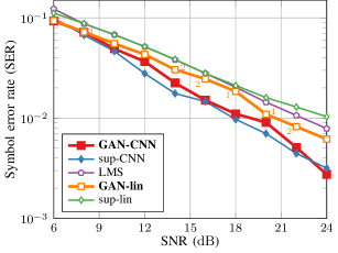
Figure 5: Results for BPSK transmission over the ProB AWGN channel with ISI — GAN: $\epsilon_{\mathrm{lr}}|_{\mathrm{G}}=0.001$, $\epsilon_{\mathrm{lr}}|_{\mathrm{D}}=0.0005$; LMS: $\epsilon_{\mathrm{lr}}=0.01$; supervised (sup): $\epsilon_{\mathrm{lr}}|_{\mathrm{CNN}}=0.005$, $\epsilon_{\mathrm{lr}}|_{\mathrm{lin}}=0.001$. If applicable, a small digit next to a marker depicts the number of non-converged runs per 5 simulation runs.

The results for the linear AWGN channel with ISI are depicted in Fig. 5. As stated in [14, Ch. 9.4-3], nonlinear equalizers have advantages in the ProB channel, which has zeros in its frequency response. The GAN-CNN is able to use these and significantly outperforms linear (non-blind) equalizers. In fact, it even follows the track of the non-blind sup-CNN without failing to converge. Interestingly, the GAN-lin significantly outperforms the other equalizers based on the same linear filters (sup-lin and LMS) by one to two dB, so the GAN may have the better training objective as state-of-the-art linear equalizers for channels with zeros in its frequency response; however, it fails to converge in some cases.

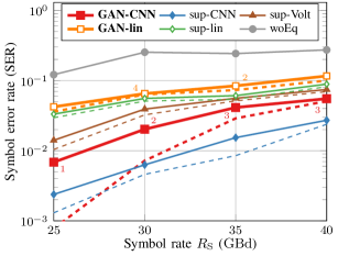
Figure 6: Results for PAM-2 transmission over an IM/DD channel with $L_{\mathrm{fiber}}=$30\text{\,}\mathrm{km}$$, ${\mathsf{SNR}}=$20\text{\,}\mathrm{d}\mathrm{B}$$ — GAN: $\epsilon_{\mathrm{lr}}|_{\mathrm{G}}=0.001$, $\epsilon_{\mathrm{lr}}|_{\mathrm{D}}=0.001$; sup: $\epsilon_{\mathrm{lr}}|_{\mathrm{CNN}}=0.0005$, $\epsilon_{\mathrm{lr}}|_{\mathrm{lin}}=0.005$, $\epsilon_{\mathrm{lr}}|_{\mathrm{Volt}}=0.007$. Depicted is the mean SER (—–), the minimum SER (- - -), and the number of non-converged runs per 5 simulation runs.

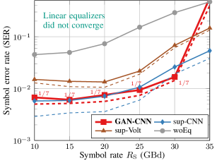
Figure 7: Results for PAM-4 transmission over an IM/DD channel with $L_{\mathrm{fiber}}=$15\text{\,}\mathrm{km}$$, ${\mathsf{SNR}}=$26\text{\,}\mathrm{d}\mathrm{B}$$ — GAN: $\epsilon_{\mathrm{lr}}|_{\mathrm{G}}=0.001$, $\epsilon_{\mathrm{lr}}|_{\mathrm{D}}=0.001$; sup: $\epsilon_{\mathrm{lr}}=0.002|_{\mathrm{CNN}}$, $\epsilon_{\mathrm{lr}}|_{\mathrm{Volt}}=0.003$. Depicted is the mean SER (—–), the minimum SER (- - -), and the number of non-converged runs per 7 simulation runs.

The results for PAM-2 transmission over the IM/DD channel are depicted in Fig. 6 for multiple symbol rates. The proposed GAN-CNN is following the non-blind sup-CNN’s track with a significant penalty, but still outperforms the other non-blind reference algorithms; however, the convergence is not as reliable as for the linear channel. Nevertheless, the minimum SER is similar to (or even better as) the sup-CNN’s minimum SER, which proves the concept and motivates further research on stabilizing the GAN training. In this nonlinear channel, the GAN-lin is not able to outperform the baseline non-blind linear equalizers, but converges to their performance.

The GAN-CNN is also able to converge for multi-amplitude modulation formats, as proven in Fig. 7 for PAM-4 transmission. For symbol rates below $35\text{\,}\mathrm{GBd}$, the GAN-CNN reaches the same performance or even outperforms (for $30\text{\,}\mathrm{GBd}$) the non-blind sup-CNN. The non-blind Volterra (sup-Volt) equalizer faces a significant penalty to the CNN-based equalizers, although both the Volterra and CNN structures have a comparable number of optimizable parameters $N_{\mathrm{param}}$ (354 vs. 333). For multi-amplitude formats, where the nonlinearities have a greater impact, the linear equalizers do not converge anymore. The cause for the GAN-CNN’s performance deterioration at $35\text{\,}\mathrm{GBd}$ is part of our ongoing investigations.

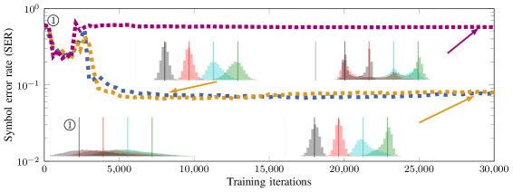
Figure 8: Convergence behavior of the GAN-CNN for PAM-4 transmission over an IM/DD channel with $R_{\mathrm{S}}=$25\text{\,}\mathrm{GBd}$$, $L_{\mathrm{fiber}}=$15\text{\,}\mathrm{km}$$, ${\mathsf{SNR}}=$20\text{\,}\mathrm{d}\mathrm{B}$$, and $\epsilon_{\mathrm{lr}}|_{\mathrm{G}}=0.001$, $\epsilon_{\mathrm{lr}}|_{\mathrm{D}}=0.001$. Depicted are three training runs and selected histograms of the equalizer output $\bm{z}$ at different training states. The light vertical lines represent the positions of the transmitted symbols with the corresponding color coding.

The convergence behaviour of three different runs is depicted in Fig. 8 for PAM-4 transmission. Histograms of the generator output $\bm{z}$ highlight the issues during training, i.e., the misclassification of the symbols in the violet (not-converged) curve. Precisely, the transmit symbols are not bijectively projected to a single but to multiple output symbols, e.g., the first (black) transmit symbol is projected to the first, second and third symbol level at the output. From a theoretical perspective, the system optimized its objective $P\left(\hat{\bm{x}}\right)=P\left(\bm{x}\right)$ but violated the requirement $(i)$ of (1).

In summary, the presented results demonstrate the high potential of our approach to improve state-of-the-art equalization in terms of flexibility, automation and communication performance. Even though the GAN-based equalizer operates blindly, i.e., without any knowledge of the transmitted symbols, results show that it can converge to—or even outperform—the supervised baselines. This allows to decrease the overhead and to increase the achievable information rate, which is crucial for modern communication systems.

V Conclusion

In this work, we have proposed a novel approach for blind and channel-agnostic equalization, and proved the concept’s feasibility. In simulations of both linear and non-linear channels with different modulation formats, we are able to demonstrate the approach’s flexibility and potential to converge towards the performance of non-blind reference equalizers. We want to highlight that the proposed equalizer is adaptive and can be used for time-varying channels, which is part of our ongoing investigations. Although challenges like training instability are not yet fully solved, the results and the theoretical analysis show that the novel concept can potentially outperform state-of-the-art equalizers while being blind and channel-agnostic. Thus, the proposed equalizer in this work is highly relevant for future research and is a next step towards integrating deep learning into communication systems.

References

- [1] D. Godard, “Self-recovering equalization and carrier tracking in two-dimensional data communication systems,” IEEE Trans. Commun., vol. 28, no. 11, pp. 1867–1875, 1980.
- [2] I. Goodfellow, J. Pouget-Abadie, M. Mirza, B. Xu, D. Warde-Farley, S. Ozair, A. Courville, and Y. Bengio, “Generative adversarial nets,” in Proc. NeurIPS, 2014.
- [3] A. Antoniou, A. Storkey, and H. Edwards, “Data augmentation generative adversarial networks,” in Proc. ICLR, 2018.
- [4] T. Karras, T. Aila, S. Laine, and J. Lehtinen, “Progressive growing of GANs for improved quality, stability, and variation,” in Proc. ICLR, 2018.
- [5] A. Brock, J. Donahue, and K. Simonyan, “Large scale GAN training for high fidelity natural image synthesis,” in Proc. ICLR, 2019.
- [6] Y. Yang, Y. Li, W. Zhang, F. Qin, P. Zhu, and C.-X. Wang, “Generative-adversarial-network-based wireless channel modeling: Challenges and opportunities,” IEEE Commun. Mag., vol. 57, no. 3, pp. 22–27, 2019.
- [7] L. Sun, Y. Wang, A. L. Swindlehurst, and X. Tang, “Generative-adversarial-network enabled signal detection for communication systems with unknown channel models,” IEEE J. Sel. Areas Commun., vol. 39, no. 1, pp. 47–60, 2021.
- [8] B. Karanov, M. Chagnon, V. Aref, D. Lavery, P. Bayvel, and L. Schmalen, “Concept and experimental demonstration of optical IM/DD end-to-end system optimization using a generative model,” in Proc. OFC, 2020.
- [9] H. Yang, Z. Niu, S. Xiao, J. Fang, Z. Liu, D. Fainsin, and L. Yi, “Fast and accurate optical fiber channel modeling using generative adversarial network,” J. Lightw. Technol., vol. 39, no. 5, pp. 1322–1333, 2021.
- [10] H. T. Nguyen, S. Bottone, K. T. Kim, M. Chiang, and H. V. Poor, “Adversarial neural networks for error correcting codes,” in Proc. GLOBECOM, 2021.
- [11] D. P. Kingma and J. Ba, “Adam: A method for stochastic optimization,” in Proc. ICLR, 2015.
- [12] T. Salimans, I. Goodfellow, W. Zaremba, V. Cheung, A. Radford, X. Chen, and X. Chen, “Improved techniques for training GANs,” in Proc. NeurIPS, 2016.
- [13] S. Ioffe and C. Szegedy, “Batch normalization: Accelerating deep network training by reducing internal covariate shift,” in PMLR, 2015.
- [14] J. Proakis and M. Salehi, Digital Communications, 5th edition. McGraw-Hill Higher Education, 2008.
- [15] D. Plabst, F. J. García Gómez, T. Wiegart, and N. Hanik, “Wiener filter for short-reach fiber-optic links,” IEEE Commun. Lett., vol. 24, no. 11, pp. 2546–2550, 2020.
- [16] G. P. Agrawal, Fiber-Optic Communication Systems, 4th edition. John Wiley & Sons, 2010.
- [17] N. Stojanovic, F. Karinou, Z. Qiang, and C. Prodaniuc, “Volterra and Wiener equalizers for short-reach 100G PAM-4 applications,” J. Lightw. Technol., vol. 35, no. 21, pp. 4583–4594, 2017.